Multiscale modeling of glioma pseudopalisades:contributions from the tumor microenvironment

Pawan Kumar1, Jing Li2, and Christina Surulescu1

1 TU Kaiserslautern, Felix-Klein-Zentrum fur Mathematik,

Paul-Ehrlich-Str. 31, 67663 Kaiserslautern, Germany2 College of Science, Minzu University of China,

Beijing, 100081, P.R. China

(kumar, surulescu@mathematik.uni-kl.de, 2010023@muc.edu.cn)

July 13, 2020

Abstract

Gliomas are primary brain tumors with a high invasive potential and infiltrative spread.Among them, glioblastoma multiforme (GBM) exhibits microvascular hyperplasia andpronounced necrosis triggered by hypoxia. Histological samples showing garland-likehypercellular structures (so-called pseudopalisades) centered around the occlusion site ofa capillary are typical for GBM and hint on poor prognosis of patient survival. Wepropose a multiscale modeling approach in the kinetic theory of active particlesframework and deduce by an upscaling process a reaction-diffusion model with repellentpH-taxis. We prove existence of a unique global bounded classical solution for a versionof the obtained macroscopic system and investigate the asymptotic behavior of thesolution. Moreover, we study two different types of scaling and compare the behavior ofthe obtained macroscopic PDEs by way of simulations. These show that patterns1

(including pseudopalisades) can be formed for some parameter ranges, in accordance withthe tumor grade. This is true when the PDEs are obtained via parabolic scaling(undirected tissue), while no such patterns are observed for the PDEs arising by ahyperbolic limit (directed tissue). This suggests that brain tissue might be undirected - atleast as far as glioma migration is concerned. We also investigate two different ways ofincluding cell level descriptions of response to hypoxia and the way they are related.

Keywords: Glioblastoma, pseudopalisade patterns, hypoxia-induced tumor behavior, kinetictransport equations, upscaling, reaction-diffusion-taxis equations, global existence, uniqueness, longtime behavior, multiscale modeling, directed/undirected tissue

1not necessarily of Turing type

1

arX

iv:2

007.

0529

7v1

[q-

bio.

TO

] 1

0 Ju

l 202

0

1 Introduction

Classified as grade IV astrocytoma by WHO [38], glioblastoma multiforme (GBM) is considered to bethe most aggressive type of glioma, with a median overall survival time of 60 weeks, in spite ofstate-of-the-art treatment [51, 62]. It is characterized by fast, infiltrative spread and unchecked cellproliferation which triggers hypoxia and upregulation of glycolysis, usually accompanied locally byexuberant angiogenesis [7, 20]; one of the typical features of GBM is the development of a necroticcore [38]. Increased extracellular pressure from edema and expression of procoagulant factorsputatively lead to vasoocclusion and thrombosis [10], hence impairing oxygen supply at the affectedsite, which becomes hypoxic and induces tissue necrotization. As a consequence, glioma cells activelyand radially migrate away from the acidic area [8], forming palisade-like structures exhibitingarrangements of elongated nuclei stacked in rows at the periphery of the hypocellular region around theocclusion site [61]. Such histopathological patterns are typically observed in GBM and are used as anindicator of tumor aggressiveness [9, 33]. Pseudopalisades can be narrow, with a width less than100 µm and a fibrillar interior structure, medium-sized (200−400 µm wide) with central necrosis andvacuolization, but with a fibrillar zone in the immediate interior proximity of the hypercellulargarland-like formation. Finally, the largest ones exceed 500 µm in width and are surrounding extensivenecrotic areas, most often containing central vessels [8].

Mathematical modeling has become a useful means for supporting the investigation of gliomadynamics in interaction with the tumor microenvironment. Over the years several modeling approacheshave been proposed. While discrete and hybrid models (see e.g. [5, 32, 52]) use computing power toassess the rather detailed interplay between glioma cells and their surroundings, the continuum settingsenable less expensive simulations and mathematical analysis of the resulting systems of differentialequations. Since the structure of brain tissue with its patient-specific anisotropy is (among otherfactors) essential for the irregular spread of glioma, the mathematical models should be able to includein an appropriate way such information, which is available from diffusion tensor imaging (DTI) data.The macroscopic evolution of a tumor is actually determined by processes taking places on lowerscales, thus it is important to deduce the corresponding population dynamics from descriptions of cellbehavior on mesoscopic or even subcellular levels, thereby taking into account the interactions with theunderlying anisotropic tissue and possibly further biochemical and/or biophysical traits of theextracellular space. This has been done e.g. in [15, 17–19, 29, 45] upon starting on the mesoscale fromthe kinetic theory of active particles (KTAP) framework [4] and obtaining with an adequate upscalingthe macroscopic PDEs of reaction-(myopic) diffusion(-taxis) type for the tumor dynamics. Dependingon whether the modeling process included subcellular events, these PDEs contain in their coefficientsinformation from that modeling level, thus receiving a multiscale character. It is this approach that weplan to follow here, however with the aim of obtaining cell population descriptions for thepseudopalisade formation rather than for the behavior of the whole tumor.

Mathematical models addressing glioma pseudopalisade formation are scarce; we refer to [11, 12] foragent-based approaches and to [1, 41] for continuous settings. Of the latter, [1] investigated the impactof blood vessel collapse on glioma invasion and the phenotypic switch in the migration/proliferationdichotomy. It involves a system of PDEs coupling the nonnlinear dynamics of glioma population withthat of nutrient concentration and vasculature, thus not explicitly including acidity. The PDE for theevolution of tumor cell density was obtained upon starting from a PDE/ODE system formigrating/proliferating glioma densities and performing transformations relying on severalassumptions. The work in [41] describes interactions between normoxic/hypoxic glioma, necrotictissue, and oxygen concentration. The model confirms the histological pattern behavior and shows bysimulations a traveling wave concentrically moving away from the highly hypoxic site toward lessacidic areas. The PDE system therein was set up in a heuristic manner directly on the macroscale; it

2

features reaction-diffusion equations without taxis or other drift.

In the present work we are interested in deducing effective equations for the space-time evolution ofglioma cell density in interaction with extracellular acidity (concentration of protons), therebyaccounting for the multiscality of the involved processes and for the anisotropy of brain tissue. Thededuced model should be able to reproduce pseudopalisade-like patterns and to investigate theinfluence of acidity and tissue on their behavior. The rest of this paper is organized as follows: inSection 2 we formulate our model upon starting from descriptions of cell dynamics on the microscopicand mesoscopic scales. Section 3 is concerned with obtaining the macroscopic limits of that setting; wewill investigate parabolic as well as hyperbolic upscalings, corresondingly leading to diffusion anddrift-dominated evolution, respectively, and depending on tissue properties (directed/undirected). Analternative modeling approach and its parabolic limit will be addressed as well. In Section 4 we providean assessment of parameters and functions involved in the deduced macroscopic PDE systems andperform numerical simulations, also providing a comparison between the studied modeling approaches.Section 5 is dedicated to establishing the existence and uniqueness of a global bounded classicalsolution to the macroscopic system obtained by parabolic scaling. A result concerning the asymptoticbehavior of such solution is proved as well. Finally, Section 6 contains a discussion of the obtainedresults and an outlook on further problems of interest related to GBM pseudopalisades.

2 Model set up on subcellular and mesoscopic scales

The approach in [17, 18] led to (hapto)taxis of glioma cell population on the macroscale upon takinginto account receptor binding of cells to the surrounding tissue. As such, it was a simplification ofsubcellular dynamics as considered in [30, 31, 37], where the cancer cells were supposed to interactwith the tissue and with a soluble ligand acting as a chemoattractant. The latter works, however, wereconcerned with the micro-meso-macro formulation of cancer cell evolution in dynamic interaction withthe tissue (as a mesoscopic quantity) and the ligand (obeying a nonlocal macroscopic PDE), along withthe analysis therewith, whereas here we intend to obtain a system of effective macroscopic PDEs forglioma population density in interaction with space-time dependent acidity. Here the macroscopic scaleis smaller than in the mentioned previous works: it is not the scale of the whole tumor, but that of asubpopulation, localized around one or several vasoocclusion sites in a comparatively small area of thetumor - corresponding to a histological sample. Since (see end of first paragraph in Section 1) the sizeof such samples is too small to allow a reliable assessment of underlying tissue distribution via DTI2,we do not describe a detailed cell-tissue interaction via cell activity variables as in the mentionedworks. However, tissue anisotropy might be relevant even on such lower scale, therefore we consider,instead, an artificial structure by way of some given water diffusion tensor, in order to be able to testsuch influences on the glioma pattern formation. Therefore, on the subcellular level we only accountexplicitly for interactions between extracellular acidity and glioma transmembrane units mediatingthem. The latter can be ion channels and membrane transporters ensuring proton exchange, or evenproton-sensing receptors [28].

We denote by y(t) the amount of transmembrane units occupied with protons (in the following we willcall this the activity variable, in line with the KTAP framework in [4]) and by R0 the total amount ofsuch units (ion channels, receptors, etc), which for simplicity we assume to be constant. Let S denotethe concentration of (extracellular) protons and Smax be a threshold value, which, when exceeded, leadsto cancer cell death. The corresponding binding/occupying kinetics are written

SSmax

+(R0−y)k+−−k−

y,

2the typical size of a voxel is ca. 1 mm3

3

so that we can write for the corresponding subcellular dynamics (upon rescaling y y/R0)

y = G(y,S) := k+S

Smax(1− y)− k−y, (2.1)

where k+ and k− represent the reaction rates. We denote by y∗ the steady-state of the above ODE, thuswe have

y∗ =k+S/Smax

k+S/Smax + k−=

S/Smax

S/Smax + kD, kD :=

k−k+

. (2.2)

As in [17, 18] we will consider deviations from the equilibrium of subcellular dynamics:

z := y∗− y.

Since the events on this scale are much faster than those on the mesoscopic and especially macroscopiclevels, the equilibrium is supposed to be quickly attained, so z is very small. We will use this assumptionin the subsequent calculations; as in [17, 18] it will allow us to get rid of higher order moments duringthe upscaling process, thus to close the system of moments leading to the macroscopic formulation.This assumption also allows us to ignore on this microscopic scale the time dependency of S.3 Next,we consider the path of a single cell starting at position x0 and moving with velocity v in the acidicenvironment. Since the glioma cells are supposed to move away from the highly hypoxic site, we take:

x := x0−vt,

which leads to

z =−k+(S

Smax+ kD)z−

kD/Smax

(S/Smax + kD)2 v ·∇S. (2.3)

We denote by p(t,x,v,y) the density function of glioma cells at time t , position x ∈ Rn, velocity v ∈V ⊂Rn, and with activity variable y ∈Y = (0,1). We assume as in [15,17–19,29,45] that the cells havea constant (average) speed s > 0, so that V = sSn−1, i.e. only the cell orientation is varying on the unitsphere. In terms of deviations z ∈ Z ⊂ [y∗−1,y∗] from the steady-state (we also call z activity variable)we consider for the evolution of p the kinetic transport equation (KTE)

∂t p+v ·∇p−∂z(((

k+S/Smax + k−)

z+ f ′(S)v ·∇S)

p)= L[λ (z)]p+P(S,M)p, (2.4)

where L[λ (z)]p := −λ (z)p + λ (z)∫

V K(x,v,v′p(v′))dv′ denotes the turning operator modeling cellvelocity innovations due to tissue contact guidance and acidity sensing, with λ (z) denoting the turningrate of cells. Thereby, K(x,v,v′) is a turning kernel giving the likelihood of a cell with velocity v′ tochange its velocity regime into v. We adopt the choice proposed in [23], i.e. K(x,v,v′) = q(x,v)

ωwhere

q(x, v) is the (stationary) orientation distribution of tissue fibers with ω =∫

V q(v)dv = sn−1 andv = v

|v| ∈ Sn−1. We take the turning rate as in [17]

λ (z) = λ0−λ1z≥ 0, (2.5)

where λ0 and λ1 are positive constants. The choice means that the turning rate is increasing with theamount of proton-occupied transmembrane units. The turning operator in (2.4) thus becomes

L[λ (z)]p = L[λ0]p−L[λ1]zp, (2.6)

3In fact, keeping this dependency and accounting for the correct scales during the macroscopic limit leads toomission of the arising supplementary term, so that the outcome is the same whether we do such assumption atthis step or later on.

4

with

L[λi]p(t,x,v,y) =−λi p(t,x,v,y)+λiqω

∫V

p(t,x,v,y)dv for i = 0,1. (2.7)

We also employ the notation f (S) = y∗ to emphasize that the steady-state of subcellular dynamicsdepends on the proton concentration S. The last term in (2.4) represents growth or depletion, accordingto the acidity level in the tumor microenvironment. Similarly to [18], but now accounting for the effectof acidity, we consider a source term of the form

P(S,M) := µ(M)∫

Zχ(z,z′)

(1− S

Smax

)p(t,x,v,z′)dz′, (2.8)

where χ(z,z′) represents the likelihood of cells having activity state z′ to go into activity state z uponinteracting with acidity S(t,x). In particular, χ is a kernel with respect to z, i.e.

∫Z χ(z,z′)dz = 1. The

acidity is reported again to the threshold value Smax. The growth rate µ(M) depends on the totalamount M(t,x) =

∫V∫

Z p(t,x,v,z)dzdv of glioma cells, irrespective of their orientation or activity stateand takes into account limitations by overcrowding. We will provide a concrete choice later inSubsection 4.1. Hence, the presence of tissue is supporting proliferation, which is maintained until theenvironment becomes too acidic even for tumor cells.

The above micro-meso formulation for glioma dynamics is supplemented with the evolution of acidity,described by the macroscopic PDE

St = Ds∆S+βM−αS, (2.9)

where Ds is the diffusion coefficient of protons, β is the proton production rate by tumor cells, and α

denotes the rate of acidity decay.The high dimensionality of the above setting makes the numerics too expensive, thus we aim to deducemacroscopic equations which can be solved more efficiently and, moreover, facilitate the observation ofthe glioma cell population and its patterning behavior. In order to investigate the possible effects of thetissue being directed or not4, we will perform two kinds of macroscopic limit: the parabolic one, for thediffusion-dominated case of undirected tissue, and the hyperbolic limit for directed tissue, which shouldbe drift-dominated. Both types of limits are performed in a formal way, as the rigorous processes wouldrequire analytical challenges which go beyond the aims of this note.

3 Macroscopic limits

We consider the following moments with respect to v and z:

m(t,x,v) =∫

Zp(t,x,v,z)dz M(t,x) =

∫∫V×Z

p(t,x,v,z)dzdv

mz(t,x,v) =∫

Zzp(t,x,v,z)dz Mz(t,x) =

∫∫V×Z

zp(t,x,v,z)dzdv

and neglect higher order moments w.r.t. z due to the assumption of the steady-state of subcellulardynamics being rapidly reached. Moreover, we assume p to be compactly supported in the phase spaceRn×V ×Z.

4by ’undirected’ we mean as in [23] that the fibers are symmetric along their axis and both fiber directionsare identical, while ’directed’ means unsymmetric fibers; since the common medical imaging techniques are notproviding the necessary resolution, it is actually not known whether brain tissue is directed, but such feature mightplay a role in the formation of glioma patterns

5

Integrating (2.4) w.r.t z, we get:

∂tm+∇x · (vm) =−λ0m+λ1mz +λ0qω

M−λ1qω

Mz +µ(M)

(1− S

Smax

)m (3.1)

Multiplying (2.4) by z and integrating w.r.t. z we get:

∂tmz +∇x · (vmz) =−(k+S/Smax + k−)mz− f ′(S)v ·∇S m−λ0mz +λ0qω

Mz

+µ(M)

(1− S

Smax

)∫Z

∫Z

zχ(z,z′)p(z′)dz′dz. (3.2)

In the following we denote as e.g., in [17, 23] by

Eq(x) :=∫Sn−1

θq(x,θ)dθ

Vq(x) :=∫Sn−1

(θ −Eq)⊗ (θ −Eq)q(x,θ)dθ

the mean fiber orientation and the variance-covariance matrix for the orientation distribution of tissuefibers, respectively.

3.1 Parabolic limit

In this subsection we consider the tissue to be undirected, which translates into the directionaldistribution function for tissue fibers being symmetric, i.e.

∫Sn−1 q(x,θ)dθ =

∫Sn−1 q(x,−θ)dθ . We

rescale the time and space variables by t := ε2t, x := εx. Since proliferation is much slower thanmigration, we also rescale with ε2 the corresponding term, as in [18]. For notation simplification wewill drop in the following the˜symbol from the scaled variables t and x.

Thus, from (3.1) and (3.2) we get:

ε2∂tm+ ε∇x · (vm) =−λ0m+λ1mz +λ0

qω

M−λ1qω

Mz + ε2µ(M)

(1− S

Smax

)m (3.3)

ε2∂tmz + ε∇x · (vmz) =−(k+S/Smax + k−+λ0)mz− ε f ′(S)v ·∇S m+λ0

qω

Mz

+ ε2µ(M)

(1− S

Smax

)∫Z

∫Z

zχ(z,z′)p(z′)dz′dz. (3.4)

Now, using Hilbert expansions for the moments:

m = m0 + εm1 + ε2m2 + ...

mz = mz0 + εmz

1 + ε2mz

2 + ...

M = M0 + εM1 + ε2M2 + ...

Mz = Mz0 + εMz

1 + ε2Mz

2 + ...

and identifying the equal powers of ε , we getε0:

0 =−λ0m0 +λ1mz0 +λ0

qω

M0−λ1qω

Mz0 (3.5)

0 =−(k+S/Smax + k−)mz0−λ0mz

0 +λ0qω

Mz0 (3.6)

6

ε1:

∇ · (vm0) =−λ0m1 +λ1mz1 +λ0

qω

M1−λ1qω

Mz1 (3.7)

∇ · (vmz0) =−(k

+S/Smax + k−)mz1− f ′(S)v ·∇Sm0−λ0mz

1 +λ0qω

Mz1 (3.8)

ε2:

∂tm0 +∇ · (vm1) =−λ0m2 +λ1mz2 +λ0

qω

M2−λ1Mz2 +µ(M)

(1− S

Smax

)m0 (3.9)

If we also expand µ around M0, (3.9) leads to

∂tm0 +∇ · (vm1) =−λ0m2 +λ1mz2 +λ0

qω

M2−λ1Mz2 +µ(M0)

(1− S

Smax

)m0. (3.10)

Integrating (3.6) w.r.t. v we get

0 =−(k+S/Smax + k−)Mz0−λ0Mz

0 +λ0Mz0

=⇒ Mz0 = 0 and mz

0 = 0.

Then from (3.5) we obtain m0 =qω

M0. Integrating (3.8) w.r.t. v gives

0 =−(k+S/Smax + k−)Mz1− f ′(S)∇S ·

∫V

vqω

dvM0.

The assumption of undirected tissue gives Eq = 0, thus from the above equation we obtain Mz1 = 0,

which in virtue of (3.8) implies

mz1 =

− f ′(S)v ·∇S m0

(k+S/Smax + k−+λ0).

The compact Hilbert–Schmidt operator L[λ0]m1 =−λ0m1+qω

M1 considered as in [23] on the weightedspace L2

qω

(V ) with measure dvq(v)

ω

has kernel 〈 qω〉, thus its pseudo-inverse can be taken on 〈 q

ω〉⊥, to deduce

from (3.7)

m1 =−1λ0

(∇ · (vm0)−λ1mz1) .

We summarize our hitherto information about the moments:

m0 =qω

M0 (3.11)

mz0 = Mz

0 = M1 = Mz1 = 0 (3.12)

m1 =−1λ0

(∇ · (v q

ωM0)−λ1mz

1

)(3.13)

mz1 =

− f ′(S)v ·∇S m0

(k+S/Smax + k−+λ0). (3.14)

Now integrating (3.10) w.r.t. v we obtain∫V

(∂t

( qω

M0

)+∇ · (vm1)

)dv = µ(M0)

(1− S

Smax

)∫V

m0dv

Using (3.11)-(3.14), the previous equation becomes

∂tM0 = ∇∇ : (DT (x)M0)+∇ · (g(S)DT (x)∇S M0)+µ(M0)

(1− S

Smax

)M0, (3.15)

7

where:g(S) = λ1(k+S/Smax + k−+λ0)

−1 f ′(S),

f (S) =S/Smax

S/Smax + kD,

u(x) =1

λ0ω

∫V

v⊗v∇q(x, v)dv = ∇ ·DT (x),

DT (x) =1

λ0ω

∫V

q(x, v)v⊗vdv.

This macroscopic PDE forms together with (2.9) the system characterizing glioma evolution under theinfluence of acidity. It involves a term describing repellent pH-taxis (the glioma cells move away fromlarge acidity gradients), in which the tactic sensitivity function contains the tumor diffusion tensor DT

encoding information about the anisotropy of underlying tissue and the function g(S) which relates tothe subcellular dynamics of proton sensing and transfer accros cell membranes. The myopic diffusion

∇∇ : (DT (x)M0) = ∇ · (DT (x)∇M0 +u(x)M0)

is common to this and previous models [17, 18, 29, 45] obtained by parabolic scaling from the KTAPframework.

An alternative approach to including acidity effects

In the previous derivation the term with repellent pH-taxis was obtained as a consequence of includingsubcellular level dynamics in the mesoscopic KTE (2.4) by way of the transport term w.r.t. the activityvariable z and by letting the turning rate depend on it. In the context of bacteria motion an alternativeapproach was proposed in [44] and re-employed in [39] also for eukaryotes having a more complexmotility behavior. It does not explicitly include subcellular dynamics (thus no activity variables andcorresponding transport terms are considered), but lets instead the cell turning rate depend on thepathwise gradient of some chemoattractant concentration which is supposed to bias the cell motion.The relationship between the two mesoscopic modeling approaches was studied for bacteria dispersalin [47], where it was rigorously shown that the alternative approach follows from the former one, undercertain assumptions made on the receptor binding dynamics on the subcellular level (along with fastrelaxation towards equilibrium of external signal transduction and stiff response of the activityvariables), on the turning rate, and on the initial data.

Here we intend to investigate two such approaches for the problem at hand (glioma cells moving awayfrom acidity) from a less rigorous perspective, namely looking into their (formal) macroscopic limitsand comparing the numerical results obtained therewith. Concretely, we want to compare our KTE (2.4)and its parabolic limit with the following simpler KTE for the cell density function ρ(t,x,v):

∂tρ +∇x · (vρ) = L[λ (v,S)]ρ +P(M,S)ρ

=−∫

Vλ (v,S)

q(v′)ω

ρ(t,x,v)dv′+∫

Vλ (v′,S)

q(v)ω

ρ(t,x,v′)dv′+P(M,S)ρ

=−λ (v,S)ρ(t,x,v)+q(v)

ω

∫V

λ (v′,S)ρ(t,x,v′)dv′+P(M,S)ρ (3.16)

and its parabolic limit. Here the proliferation operator is defined with the same µ(M,S) as previouslyused in this section and takes the form

P(M,S) = µ(M,S)ρ, (3.17)

8

while for the turning rate we set5

λ (v,S) := λ0 exp(h(S)DtS) (3.18)

' λ0(1+h(S)DtS), (3.19)

where DtS := St + v ·∇xS is the pathwise gradient of S. The coefficient function h(S) is to be chosenlater.

We use again a parabolic scaling t := ε2t, x := εx and rescale as before the proliferation term by ε2, thus

ε2∂tρ + ε∇ · (vρ) =−λ0(1+h(S)(ε2

∂tS+ εv ·∇S))ρ +λ0qω

(M+h(S)(ε2

∂tS M+ ε

∫V

v′ρ(v′)dv′ ·∇S))

+ ε2P(M,S)ρ. (3.20)

Performing a Hilbert expansion ρ = ρ0 + ερ1 + ε2ρ2 + . . . and equating the powers of ε yields

ε0:

0 =−λ0ρ0 +λ0q(x, v)

ωM0,

thus

ρ0 =q(v)

ωM0. (3.21)

ε1:

∇ · (vρ0) =−λ0ρ1−λ0h(S)ρ0v ·∇S+λ0qω

(M1 +h(S)

∫V

v′ρ0(v′)dv′ ·∇S),

thus by (3.21) and the assumption of undirected tissue

∇ · (vq(v)ω

M0) =−λ0ρ1−λ0h(S)qω

M0v ·∇S+λ0qω

M1. (3.22)

This can be rewritten as

L[λ0]ρ1 = λ0h(S)qω

M0v ·∇S+∇ · (vq(v)ω

M0). (3.23)

Since the integral of the right hand side w.r.t. v vanishes we can pseudo-invert L[λ0] as before, to get

ρ1 =−h(S)qω

M0v ·∇S− 1λ0

∇ · (vq(v)ω

M0). (3.24)

ε2:

∂tρ0 +∇ · (vρ1) = λ0(qω

M2−ρ2)+λ0h(S)∂tS (qω

M0−ρ0)+λ0h(S)(

qω

∫V

v′ρ1(v′)dv′−v)·∇S

+µ(M0,S)ρ0. (3.25)

Integrating (3.25) w.r.t v gives

∂tM0 +∇ ·∫

Vvρ1dv = µ(M0,S)M0.

5notice the difference of sign in the exponent: the cells are supposed to follow the decreasing gradient of signalS

9

Using (3.24) leads to

∂tM0 = ∇∇ : (DT M0)+∇ · (λ0h(S)DT M0∇S)+µ(M0,S)M0, (3.26)

which differs from (3.15) only by the tactic sensitivity coefficient. This suggests to choose

h(S) =g(S)λ0

=λ1

λ0

f ′(S)k+S/Smax + k−+λ0

.

Notice that this function corresponds to the rate of change of f (S) (equilibrium of transmembraneinteractions between glioma cells and acidity), scaled by a constant λ1 to account for changes in theturning rate per unit of change in dy∗/dt, and multiplied by 1/(k+S/Smax + k−+ λ0). While a factorconst · f ′(S) is also encountered in [44], the denominator obtained here for the tactic sensitivity appearsdue to the specific choice of the turning rate λ (z) in (2.5), which also facilitated the upscaling. Thewhole sensitivity function is tightly related to the first order moment w.r.t. the receptor binding(’activity’) variable z, recall (3.12) and (3.14).

3.2 Hyperbolic scaling

In this subsection we investigate the macroscopic limit of (2.4) in the case where the tissue is directed.In particular, this means that the mean fiber orientation Eq is nonzero, as the orientation distribution qis unsymmetric. We will only treat the case explicitly accounting for the dynamics of activity variables.

Consider on L2qω

(V ) =< q/ω > ⊕ < q/ω >⊥ the Chapman-Enskog expansion of the cell distributionfunction p(t,x,v,z) in the form

p(t,x,v,z) = p(t,x,z)qω(x, v)+ ε p⊥(t,x,v,z), (3.27)

where∫

V p⊥(t,x,v,z)dv = 0 and p(t,x,z) :=∫

V p(t,x,v,z)dv. Then for the moments introduced at thebeginning of this Section 3 we have

m(t,x,v) =∫

Zp(t,x,v,z)dz =

∫Z

p(t,x,z)q(x, v)

ωdz+ ε

∫Z

p⊥(t,x,v,z)dz

=:q(x, v)

ωM(t,x)+ εm⊥(t,x,v)

mz(t,x,v) =∫

Zzp(t,x,v,z)dz =

q(x, v)w

∫Z

zp(t,x,z)dz+ ε

∫Z

zp⊥(t,x,v,z)dz

=:q(x, v)

ωMz(t,x)+ εmz

⊥(t,x,v).

(3.28)

Now we rescale the time and space variables by t := εt, x := εx and drop again the˜symbol to simplifythe notation. As before, the proliferation term is scaled by ε2. With these, the equations (3.1) and (3.2)become, respectively:

ε∂tm+ ε∇x · (vm) =−λ0m+λ1mz +λ0qω

M−λ1qω

Mz + ε2µ(M)

(1− S

Smax

)m (3.29)

and

ε∂tmz + ε∇x · (vmz) =−(k+S/Smax + k−)mz− ε f ′(S)v ·∇S m−λ0mz +λ0qω

Mz

+ ε2µ(M)

(1− S

Smax

)∫Z

∫Z

zχ(z,z′)p(z′)dz′dz. (3.30)

10

Using (3.28) we write

ε∂t

( qω

M+ εm⊥)+ ε∇ · (v

( qω

M+ εm⊥)) =−λ0

( qω

M+ εm⊥)+λ1

( qω

Mz + εmz⊥

)+λ0

qω

M−λ1qω

Mz + ε2µ(M)

(1− S

Smax

)m (3.31)

ε∂t

( qω

Mz + εmz⊥

)+ ε∇ · (v

( qω

Mz + εmz⊥

)) =−(k+S/Smax + k−)

( qω

Mz + εmz⊥

)− ε f ′(S)v ·∇S

( qω

M+ εm⊥)−λ0

( qω

Mz + εmz⊥

)+λ0

qω

Mz

+ ε2µ(M)

(1− S

Smax

)∫Z

∫Z

zχ(z,z′)p(z′)dz′dz. (3.32)

Since q is independent of time, these equations imply

qω

∂tM+ ε∂tm⊥+∇ · (vMqω)+ ε∇ · (vm⊥) =−λ0m⊥+λ1mz

⊥+ εµ(M)

(1− S

Smax

)m (3.33)

εqω

∂tMz + ε2∂tmz

⊥+ ε∇ · (vMz qω)+ ε

2∇ · (vmz

⊥) =−(k+S/Smax + k−)

qω

Mz− ε(k+S/Smax + k−)mz⊥

− ε f ′(S)v ·∇Sqω

M− ε2 f ′(S)v ·∇S m⊥− ελ0mz

⊥

+ ε2µ(M)

(1− S

Smax

)∫Z

∫Z

zχ(z,z′)p(z′)dz′dz.

(3.34)

Integrating (3.33) w.r.t. v gives

∂tM+∇ · (EqM)+ ε∇ ·∫

Vvm⊥dv = εµ(M)

(1− S

Smax

)M, (3.35)

where we used the notation Eq(x) :=∫

V v qω(x, v)dv = sEq.

From (3.34) we get at leading order

−(k+S/Smax + k−)qω

Mz = 0 ⇒ Mz = 0.

Plugging this in (3.34), we obtain (again at leading order)

0 =−(k+S/Smax + k−)mz⊥− f ′(S)v ·∇S

qω

M−λ0mz⊥,

whence

mz⊥ =

− f ′(S)v ·∇Sk+S/Smax + k−+λ0

qω

M. (3.36)

From (3.35):

∂tM = εµ(M)

(1− S

Smax

)M−∇ · (EqM)− ε∇ ·

∫V

vm⊥dv. (3.37)

Plugging this into (3.33) we get (at leading order)

L[λ0]m⊥ =− qω

∇ ·(EqM

)+∇ · (vM

qω)−λ1mz

⊥. (3.38)

11

Since the right hand side vanishes when integrated w.r.t. v, we can pseudo-invert L[λ0] and use (3.36)to get

m⊥ =−1λ0

(∇ ·(

vMqω

)− q

ω∇ ·(EqM

)−λ1

− f ′(S)v ·∇Sk+S/Smax + k−+λ0

qω

M), (3.39)

hence

∇ ·∫

Vvm⊥dv =−∇∇ : (DT M)+∇ ·

(1λ0

Eq∇ · (EqM)

)−λ1∇ ·

(f ′(S)

k+S/Smax + k−+λ0DT M∇S

),

(3.40)

so that (3.35) becomes

∂tM+∇ · (sEqM) = ε∇∇ : (DT M)− ε∇ ·(

s2

λ0Eq∇ · (EqM)

)+ ε∇ · (g(S)DT M∇S)

+ εµ(M)

(1− S

Smax

)M. (3.41)

Comparing this with the parabolic limit obtained in (3.15) we observe that we obtain the same form forthe (myopic) diffusion, repellent pH-taxis, and proliferation terms, but here they are ε-corrections of theleading transport terms - together with the new advection which drives cells with velocity ε

λ0Eq∇ ·Eq in

the direction of the dominating drift.

4 Numerical simulations

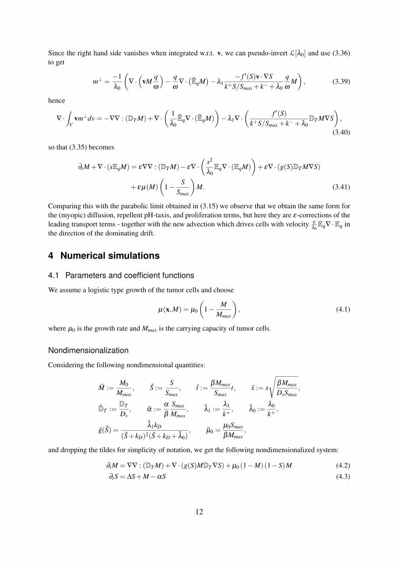
4.1 Parameters and coefficient functions

We assume a logistic type growth of the tumor cells and choose

µ(x,M) = µ0

(1− M

Mmax

), (4.1)

where µ0 is the growth rate and Mmax is the carrying capacity of tumor cells.

Nondimensionalization

Considering the following nondimensional quantities:

M :=M0

Mmax, S :=

SSmax

, t :=βMmax

Smaxt, x := x

√βMmax

DsSmax,

DT :=DT

Ds, α :=

α

β

Smax

Mmax, λ1 :=

λ1

k+, λ0 :=

λ0

k+,

g(S) =λ1kD

(S+ kD)2(S+ kD + λ0), µ0 =

µ0Smax

βMmax,

and dropping the tildes for simplicity of notation, we get the following nondimensionalized system:

∂tM = ∇∇ : (DT M)+∇ · (g(S)MDT ∇S)+µ0 (1−M)(1−S)M (4.2)

∂tS = ∆S+M−αS (4.3)

12

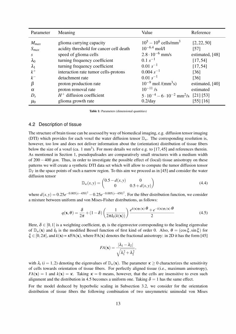
Parameter Meaning Value Reference

Mmax glioma carrying capacity 105−108 cells/mm3 [2, 22, 50]Smax acidity threshold for cancer cell death 10−6.4 mol/l [57]s speed of glioma cells 2.8 ·10−6 mm/s estimated, [48]λ0 turning frequency coefficient 0.1 s−1 [17, 54]λ1 turning frequency coefficient 0.01 s−1 [17, 54]k+ interaction rate tumor cells-protons 0.004 s−1 [36]k− detachment rate 0.01 s−1 [36]β proton production rate 10−9 mol /(mm3s) estimated, [40]α proton removal rate 10−11 /s estimatedDs H+ diffusion coefficient 5 ·10−4−6 ·10−2 mm2/s [21] [53]µ0 glioma growth rate 0.2/day [55] [16]

Table 1: Parameters (dimensional quantities)

4.2 Description of tissue

The structure of brain tissue can be assessed by way of biomedical imaging, e.g. diffusion tensor imaging(DTI) which provides for each voxel the water diffusion tensor Dw. The corresponding resolution is,however, too low and does not deliver information about the (orientation) distribution of tissue fibersbelow the size of a voxel (ca. 1 mm3). For more details we refer e.g. to [17, 45] and references therein.As mentioned in Section 1, pseudopalisades are comparatively small structures with a medium widthof 200− 400 µm. Thus, in order to investigate the possible effect of (local) tissue anisotropy on thesepatterns we will create a synthetic DTI data set which will allow to compute the tumor diffusion tensorDT in the space points of such a narrow region. To this aim we proceed as in [45] and consider the waterdiffusion tensor

Dw(x,y) =(

0.5−d(x,y) 00 0.5+d(x,y)

)(4.4)

where d(x,y) = 0.25e−0.005(x−450)2−0.25e−0.005(y−450)2. For the fiber distribution function, we consider

a mixture between uniform and von Mises-Fisher distributions, as follows:

q(x,θ) =δ

2π+(1−δ )

(1

2πI0(k(x))

)ek(x)ϕ1(x)·θ + e−k(x)ϕ1(x)·θ

2(4.5)

Here, δ ∈ [0,1] is a weighting coefficient, ϕ1 is the eigenvector corresponding to the leading eigenvalueof Dw(x) and I0 is the modified Bessel function of first kind of order 0. Also, θ = (cosξ ,sinξ ) forξ ∈ [0,2π], and k(x) = κFA(x), where FA(x) denotes the fractional anisotropy: in 2D it has the form [45]

FA(x) =|λ1−λ2|√

λ 21 +λ 2

2

,

with λi (i = 1,2) denoting the eigenvalues of Dw(x). The parameter κ ≥ 0 characterizes the sensitivityof cells towards orientation of tissue fibers. For perfectly aligned tissue (i.e., maximum anisotropy),FA(x) = 1 and k(x) = κ . Taking κ = 0 means, however, that the cells are insensitive to even suchalignment and the distribution in 4.5 becomes a uniform one. Taking δ = 1 has the same effect.

For the model deduced by hyperbolic scaling in Subsection 3.2, we consider for the orientationdistribution of tissue fibers the following combination of two unsymmetric unimodal von Mises

13

distributions:

qh(x,θ) =δ

2πI0(kh(x))ekh(x)γ·θ +

1−δ

2πI0(k(x))ek(x)ϕ1·θ , (4.6)

where kh(x) = 0.05e−10−6((x−450)2+(y−450)2), γ =(

1/√

2,1/√

2)T

and the rest of parameters are thesame as in (4.5). The first summand, similar to the choice in [24], generates an orientation along thediagonal γ , while the second leads to alignment along the positive x and y directions. Due to kh(x), thestrength of diagonal orientation of tissues decreases from the chosen center (450,450).

The macroscopic tissue density Q is obtained in the same way as in [18] by using the free path lengthfrom the diffusivity obtained from the data, more precisely from the water diffusion tensor. In thatapproach the occupied volume is obtained upon computing a characteristic (diffusion) lengthlc =

√tr(Dw)tc, where tc is the characteristic (diffusion) time. The latter is determined by assuming the

underlying stochastic process behind water diffusion tensor measurements to be the Brownian motionand considering the expected exit time from the minimal ball with radius r containing a square withside length h as smallest unit in our grid. Therefore, the tissue density Q (area fraction occupied bytissue) is:

Q = 1− l2c

h2 , (4.7)

where

lc =

√tr (Dw)h2

4l1

with l1 being the largest eigenvalue of Dw.

4.3 Numerical experiments

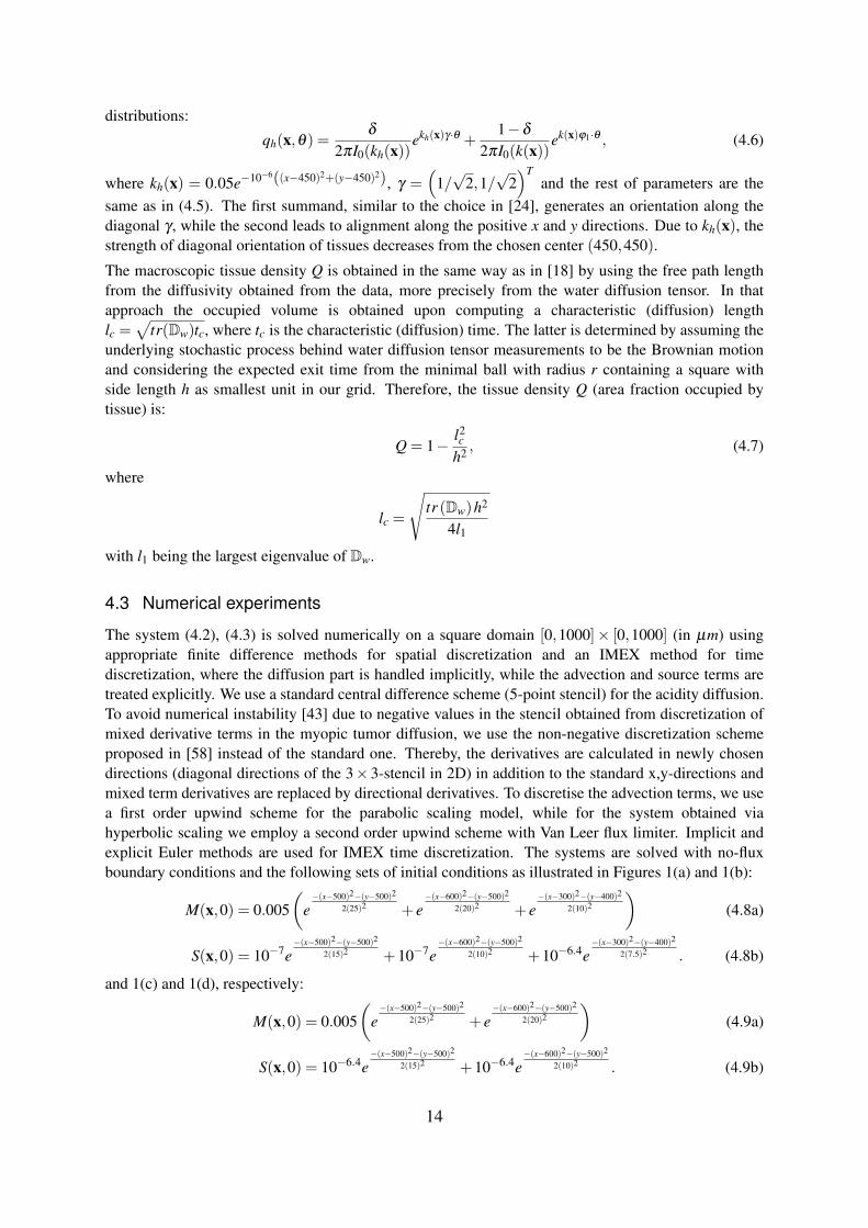
The system (4.2), (4.3) is solved numerically on a square domain [0,1000]× [0,1000] (in µm) usingappropriate finite difference methods for spatial discretization and an IMEX method for timediscretization, where the diffusion part is handled implicitly, while the advection and source terms aretreated explicitly. We use a standard central difference scheme (5-point stencil) for the acidity diffusion.To avoid numerical instability [43] due to negative values in the stencil obtained from discretization ofmixed derivative terms in the myopic tumor diffusion, we use the non-negative discretization schemeproposed in [58] instead of the standard one. Thereby, the derivatives are calculated in newly chosendirections (diagonal directions of the 3×3-stencil in 2D) in addition to the standard x,y-directions andmixed term derivatives are replaced by directional derivatives. To discretise the advection terms, we usea first order upwind scheme for the parabolic scaling model, while for the system obtained viahyperbolic scaling we employ a second order upwind scheme with Van Leer flux limiter. Implicit andexplicit Euler methods are used for IMEX time discretization. The systems are solved with no-fluxboundary conditions and the following sets of initial conditions as illustrated in Figures 1(a) and 1(b):

M(x,0) = 0.005(

e−(x−500)2−(y−500)2

2(25)2 + e−(x−600)2−(y−500)2

2(20)2 + e−(x−300)2−(y−400)2

2(10)2

)(4.8a)

S(x,0) = 10−7e−(x−500)2−(y−500)2

2(15)2 +10−7e−(x−600)2−(y−500)2

2(10)2 +10−6.4e−(x−300)2−(y−400)2

2(7.5)2 . (4.8b)

and 1(c) and 1(d), respectively:

M(x,0) = 0.005(

e−(x−500)2−(y−500)2

2(25)2 + e−(x−600)2−(y−500)2

2(20)2

)(4.9a)

S(x,0) = 10−6.4e−(x−500)2−(y−500)2

2(15)2 +10−6.4e−(x−600)2−(y−500)2

2(10)2 . (4.9b)

14

(a) (b)

(c) (d)

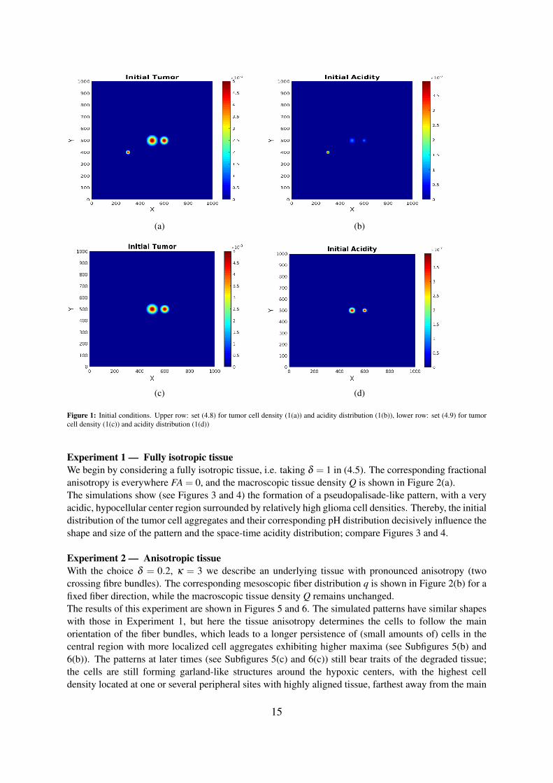
Figure 1: Initial conditions. Upper row: set (4.8) for tumor cell density (1(a)) and acidity distribution (1(b)), lower row: set (4.9) for tumorcell density (1(c)) and acidity distribution (1(d))

Experiment 1 — Fully isotropic tissueWe begin by considering a fully isotropic tissue, i.e. taking δ = 1 in (4.5). The corresponding fractionalanisotropy is everywhere FA = 0, and the macroscopic tissue density Q is shown in Figure 2(a).The simulations show (see Figures 3 and 4) the formation of a pseudopalisade-like pattern, with a veryacidic, hypocellular center region surrounded by relatively high glioma cell densities. Thereby, the initialdistribution of the tumor cell aggregates and their corresponding pH distribution decisively influence theshape and size of the pattern and the space-time acidity distribution; compare Figures 3 and 4.

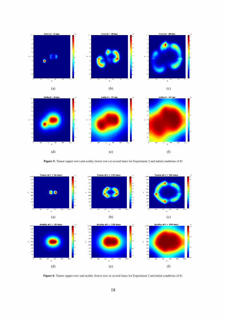
Experiment 2 — Anisotropic tissueWith the choice δ = 0.2, κ = 3 we describe an underlying tissue with pronounced anisotropy (twocrossing fibre bundles). The corresponding mesoscopic fiber distribution q is shown in Figure 2(b) for afixed fiber direction, while the macroscopic tissue density Q remains unchanged.The results of this experiment are shown in Figures 5 and 6. The simulated patterns have similar shapeswith those in Experiment 1, but here the tissue anisotropy determines the cells to follow the mainorientation of the fiber bundles, which leads to a longer persistence of (small amounts of) cells in thecentral region with more localized cell aggregates exhibiting higher maxima (see Subfigures 5(b) and6(b)). The patterns at later times (see Subfigures 5(c) and 6(c)) still bear traits of the degraded tissue;the cells are still forming garland-like structures around the hypoxic centers, with the highest celldensity located at one or several peripheral sites with highly aligned tissue, farthest away from the main

15

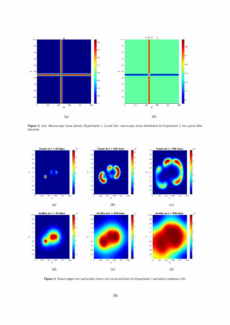
(a) (b)

Figure 2: 2(a): Macroscopic tissue density (Experiments 1, 2) and 2(b): mesoscopic tissue distribution for Experiment 2, for a given fiberdirection.

(a) (b) (c)

(d) (e) (f)

Figure 3: Tumor (upper row) and acidity (lower row) at several times for Experiment 1 and initial conditions (4.8).

16

(a) (b) (c)

(d) (e) (f)

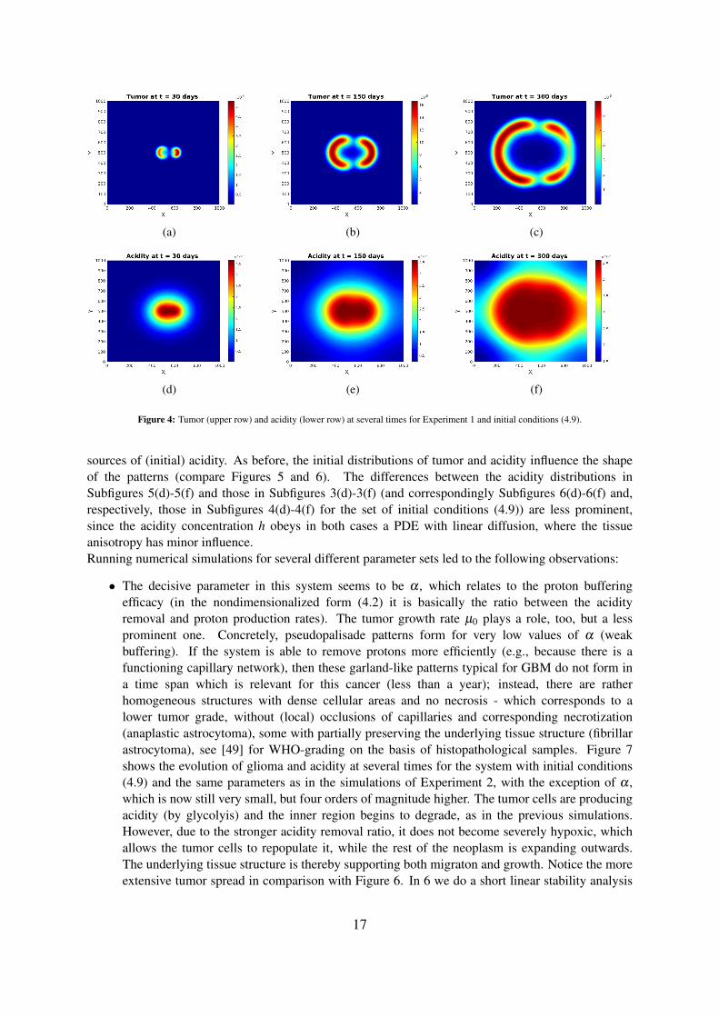
Figure 4: Tumor (upper row) and acidity (lower row) at several times for Experiment 1 and initial conditions (4.9).

sources of (initial) acidity. As before, the initial distributions of tumor and acidity influence the shapeof the patterns (compare Figures 5 and 6). The differences between the acidity distributions inSubfigures 5(d)-5(f) and those in Subfigures 3(d)-3(f) (and correspondingly Subfigures 6(d)-6(f) and,respectively, those in Subfigures 4(d)-4(f) for the set of initial conditions (4.9)) are less prominent,since the acidity concentration h obeys in both cases a PDE with linear diffusion, where the tissueanisotropy has minor influence.Running numerical simulations for several different parameter sets led to the following observations:

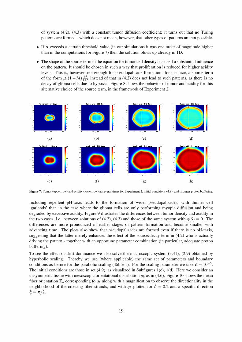
• The decisive parameter in this system seems to be α , which relates to the proton bufferingefficacy (in the nondimensionalized form (4.2) it is basically the ratio between the acidityremoval and proton production rates). The tumor growth rate µ0 plays a role, too, but a lessprominent one. Concretely, pseudopalisade patterns form for very low values of α (weakbuffering). If the system is able to remove protons more efficiently (e.g., because there is afunctioning capillary network), then these garland-like patterns typical for GBM do not form ina time span which is relevant for this cancer (less than a year); instead, there are ratherhomogeneous structures with dense cellular areas and no necrosis - which corresponds to alower tumor grade, without (local) occlusions of capillaries and corresponding necrotization(anaplastic astrocytoma), some with partially preserving the underlying tissue structure (fibrillarastrocytoma), see [49] for WHO-grading on the basis of histopathological samples. Figure 7shows the evolution of glioma and acidity at several times for the system with initial conditions(4.9) and the same parameters as in the simulations of Experiment 2, with the exception of α ,which is now still very small, but four orders of magnitude higher. The tumor cells are producingacidity (by glycolyis) and the inner region begins to degrade, as in the previous simulations.However, due to the stronger acidity removal ratio, it does not become severely hypoxic, whichallows the tumor cells to repopulate it, while the rest of the neoplasm is expanding outwards.The underlying tissue structure is thereby supporting both migraton and growth. Notice the moreextensive tumor spread in comparison with Figure 6. In 6 we do a short linear stability analysis

17

(a) (b) (c)

(d) (e) (f)

Figure 5: Tumor (upper row) and acidity (lower row) at several times for Experiment 2 and initial conditions (4.8)

(a) (b) (c)

(d) (e) (f)

Figure 6: Tumor (upper row) and acidity (lower row) at several times for Experiment 2 and initial conditions (4.9).

18

of system (4.2), (4.3) with a constant tumor diffusion coefficient; it turns out that no Turingpatterns are formed - which does not mean, however, that other types of patterns are not possible.

• If α exceeds a certain threshold value (in our simulations it was one order of magnitude higherthan in the computations for Figure 7) then the solution blows up already in 1D.

• The shape of the source term in the equation for tumor cell density has itself a substantial influenceon the pattern. It should be chosen in such a way that proliferation is reduced for higher aciditylevels. This is, however, not enough for pseudopalisade formation: for instance, a source termof the form µ0(1−M) M

1+S instead of that in (4.2) does not lead to such patterns, as there is nodecay of glioma cells due to hypoxia. Figure 8 shows the behavior of tumor and acidity for thisalternative choice of the source term, in the framework of Experiment 2.

(a) (b) (c) (d)

(e) (f) (g) (h)

Figure 7: Tumor (upper row) and acidity (lower row) at several times for Experiment 2, initial conditions (4.9), and stronger proton buffering.

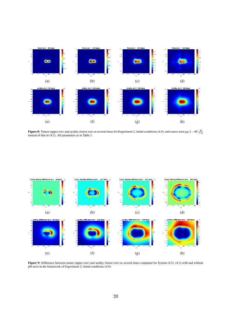
Including repellent pH-taxis leads to the formation of wider pseudopalisades, with thinner cell’garlands’ than in the case where the glioma cells are only performing myopic diffusion and beingdegraded by excessive acidity. Figure 9 illustrates the differences between tumor density and acidity inthe two cases, i.e. between solutions of (4.2), (4.3) and those of the same system with g(S) = 0. Thedifferences are more pronounced in earlier stages of pattern formation and become smaller withadvancing time. The plots also show that pseudopalisades are formed even if there is no pH-taxis,suggesting that the latter merely enhances the effect of the source/decay term in (4.2) who is actuallydriving the pattern - together with an opportune parameter combination (in particular, adequate protonbuffering).

To see the effect of drift dominance we also solve the macroscopic system (3.41), (2.9) obtained byhyperbolic scaling. Thereby we use (where applicable) the same set of parameters and boundaryconditions as before for the parabolic scaling (Table 1). For the scaling parameter we take ε = 10−5.The initial conditions are those in set (4.9), as visualized in Subfigures 1(c), 1(d). Here we consider anunsymmetric tissue with mesoscopic orientational distribution qh as in (4.6). Figure 10 shows the meanfiber orientation Eq corresponding to qh along with a magnification to observe the directionality in theneighborhood of the crossing fiber strands, and with qh plotted for δ = 0.2 and a specific directionξ = π/2.

19

(a) (b) (c) (d)

(e) (f) (g) (h)

Figure 8: Tumor (upper row) and acidity (lower row) at several times for Experiment 2, initial conditions (4.9), and source term µ0(1−M) M1+S

instead of that in (4.2). All parameters as in Table 1.

(a) (b) (c) (d)

(e) (f) (g) (h)

Figure 9: Difference between tumor (upper row) and acidity (lower row) at several times computed for System (4.2), (4.3) with and withoutpH-taxis in the framework of Experiment 2, initial conditions (4.9).

20

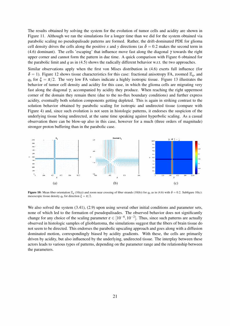
The results obtained by solving the system for the evolution of tumor cells and acidity are shown inFigure 11. Although we ran the simulations for a longer time than we did for the system obtained viaparabolic scaling no pseudopalisade patterns are formed. Rather, the drift-dominated PDE for gliomacell density drives the cells along the positive x and y directions (as δ = 0.2 makes the second term in(4.6) dominant). The cells ’escaping’ that influence move fast along the diagonal γ towards the rightupper corner and cannot form the pattern in due time. A quick comparison with Figure 6 obtained forthe parabolic limit and q as in (4.5) shows the radically different behavior w.r.t. the two approaches.

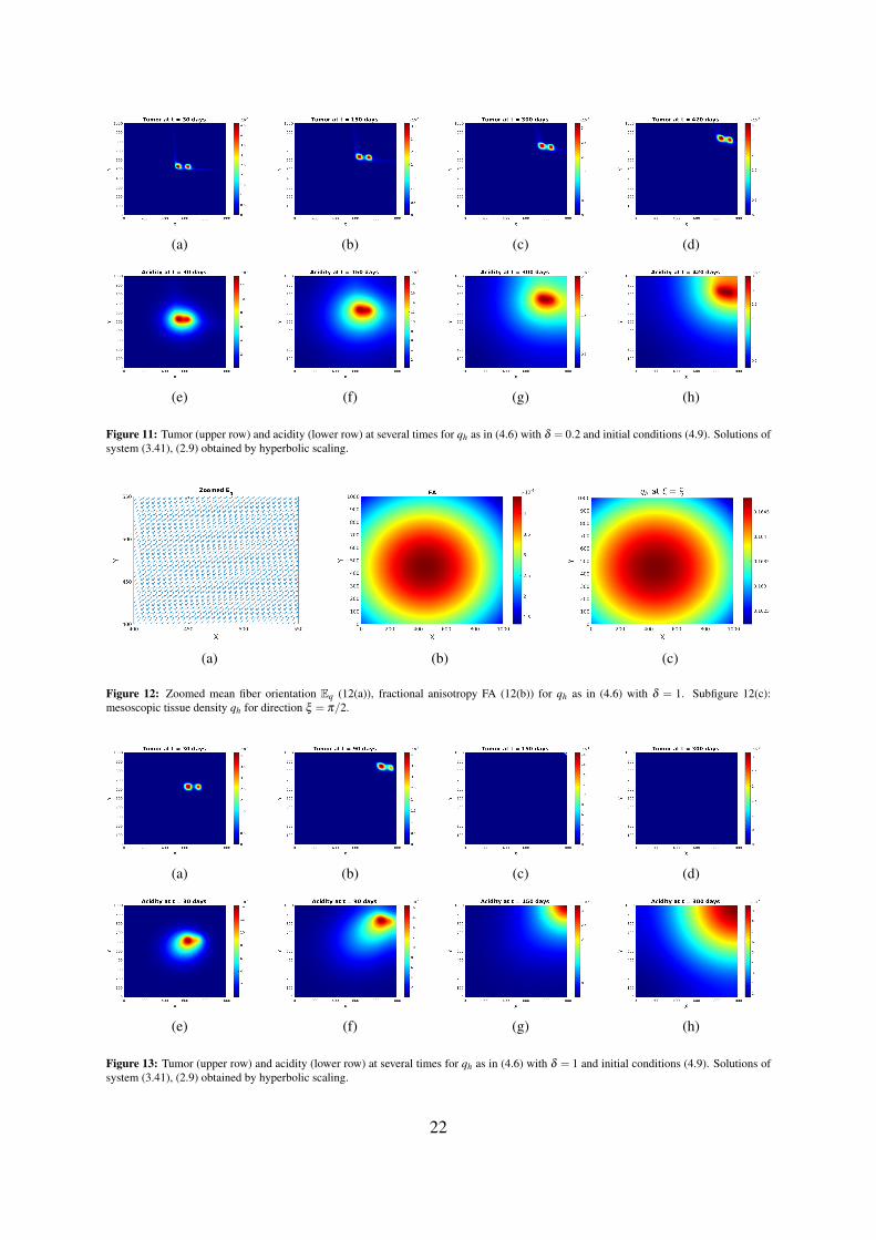
Similar observations apply when the first von Mises distribution in (4.6) exerts full influence (forδ = 1). Figure 12 shows tissue characteristics for this case: fractional anisotropy FA, zoomed Eq, andqh for ξ = π/2. The very low FA values indicate a highly isotropic tissue. Figure 13 illustrates thebehavior of tumor cell density and acidity for this case, in which the glioma cells are migrating veryfast along the diagonal γ , accompanied by acidity they produce. When reaching the right uppermostcorner of the domain they remain there (due to the no-flux boundary conditions) and further expressacidity, eventually both solution components getting depleted. This is again in striking contrast to thesolution behavior obtained by parabolic scaling for isotropic and undirected tissue (compare withFigure 4) and, since such evolution is not seen in histologic patterns, it endorses the suspicion of theunderlying tissue being undirected, at the same time speaking against hyperbolic scaling. As a casualobservation there can be blow-up also in this case, however for a much (three orders of magnitude)stronger proton buffering than in the parabolic case.

(a) (b) (c)

Figure 10: Mean fiber orientation Eq (10(a)) and zoom near crossing of fiber strands (10(b)) for qh as in (4.6) with δ = 0.2. Subfigure 10(c):mesoscopic tissue density qh for direction ξ = π/2.

We also solved the system (3.41), (2.9) upon using several other initial conditions and parameter sets,none of which led to the formation of pseudopalisades. The observed behavior does not significantlychange for any choice of the scaling parameter ε ∈ [10−6,10−2]. Thus, since such patterns are actuallyobserved in histologic samples of glioblastoma, the simulations suggest that the fibers of brain tissue donot seem to be directed. This endorses the parabolic upscaling approach and goes along with a diffusiondominated motion, correspondingly biased by acidity gradients. With these, the cells are primarilydriven by acidity, but also influenced by the underlying, undirected tissue. The interplay between theseactors leads to various types of patterns, depending on the parameter range and the relationship betweenthe parameters.

21

(a) (b) (c) (d)

(e) (f) (g) (h)

Figure 11: Tumor (upper row) and acidity (lower row) at several times for qh as in (4.6) with δ = 0.2 and initial conditions (4.9). Solutions ofsystem (3.41), (2.9) obtained by hyperbolic scaling.

(a) (b) (c)

Figure 12: Zoomed mean fiber orientation Eq (12(a)), fractional anisotropy FA (12(b)) for qh as in (4.6) with δ = 1. Subfigure 12(c):mesoscopic tissue density qh for direction ξ = π/2.

(a) (b) (c) (d)

(e) (f) (g) (h)

Figure 13: Tumor (upper row) and acidity (lower row) at several times for qh as in (4.6) with δ = 1 and initial conditions (4.9). Solutions ofsystem (3.41), (2.9) obtained by hyperbolic scaling.

22

5 Qualitative analysis of the macroscopic reaction-diffusion-taxissystem

5.1 Main results

We consider system (4.2), (4.3) with a slight modification of the source term in (4.3):Mt = ∇ · (DT (x)∇M)+∇ · ((g(S)DT (x)∇S+u(x))M)+ f (M,S), (t,x) ∈ (0,+∞)×Ω,

St = ∆S+ δM1+M −αS, (t,x) ∈ (0,+∞)×Ω,(

DT (x)∇M+u(x)M)·ν = ∇S ·ν = 0, (t,x) ∈ (0,+∞)×∂Ω,

M(0,x) = M0(x), S(0,x) = S0(x), x ∈Ω,

(5.1)

with g(S) := Λ

(S+K)2(S+K+B) and f (M,S) = µ0M(1−M)(1−S), where we use Λ = λ1kD, K = kD, andB = λ0 to denote the corresponding constants occurring in the expression of g(S) as given in Subsection4.1. Ω⊂ RN is considered to be a bounded domain with sufficiently smooth boundary ∂Ω, all involvedconstants are positive, M0 ∈ L∞(Ω), M0 6≡ 0, M0,S0 ≥ 0, and S0 ∈W 1,∞(Ω). The no-flux boundaryconditions are obtained through the upscaling procedure (as done e.g., in [14] for a related problem).For the tumor diffusion tensor DT we require

Assumption 5.1

(A) DT (x) ∈(

C2,γ(Ω)∩C(Ω))N×N

, γ ∈ (0,1), u = ∇ ·DT is uniformly bounded in Ω, and u(x) = 0for x ∈ ∂Ω;

(B) there exists ϑ > 0 such that for any ξ ∈ RN and x ∈Ω,

ξ> ·DT (x) ·ξ ≥ ϑ |ξ |2.

Theorem 5.1 Let N ≥ 1. Suppose that Assumption 5.1 holds. Then if ζ < α and ‖S0‖L∞(Ω) < 1, system(5.1) admits a unique global bounded classical solution.

Theorem 5.2 Under the assumptions of Theorem 5.1, suppose moreover that ∇ ·u(x) = 0 for all x ∈Ω.Then there exists µ∗ > 0, such that if µ0 > µ∗, for any x ∈Ω we have

limt→∞

M(t,x) = 1, limt→∞

S(t,x) =ζ

2α.

Moreover, there exists C > 0 and D > 0 such that for all t ∈ [0,+∞),

‖M(t, ·)−1‖L∞(Ω) ≤Ce−Dt

N+2 ,∥∥∥∥S(t, ·)− ζ

2α

∥∥∥∥L∞(Ω)

≤Ce−Dt

N+2 .

5.2 Global existence, uniqueness, and boundedness of solutions

Firstly, we state a result concerning local existence of classical solutions, which can be proved bywell-established methods involving standard parabolic regularity theory and an appropriate fixed pointframework. Moreover, one can thereby derive a sufficient condition for extensibility of a givenlocal-in-time solution(see [59] or [13] for example).

23

Lemma 5.1 Let Ω ⊂ RN (N ≥ 1) be a bounded domain with smooth boundary. Suppose that thenonnegative functions M0,S0 are in W 1,∞(Ω). Then there exist Tmax ∈ (0,∞] and a unique pair ofnon-negative functions (M,S) satisfying

M ∈C0([0,Tmax);C0(Ω))∩C2,1((0,Tmax)×Ω),

S ∈C0([0,Tmax);C0(Ω))∩L∞loc([0,Tmax);W 1,∞(Ω))∩C2,1((0,Tmax)×Ω),

and solving (5.1) classically in Ω× (0,Tmax). Moreover, if Tmax < ∞, then

limsupt→Tmax

(‖M(t, ·)‖L∞(Ω)+‖S(t, ·)‖W 1,∞(Ω)

)= ∞.

Next we prove results relating to the global boundedness of solutions to (5.1).

Lemma 5.2 There exists CS > 0 such that

‖S‖L∞([0,Tmax)×Ω) ≤max

ζ

α,‖S0‖L∞(Ω)

,

‖∇S‖L∞([0,Tmax)×Ω) ≤CS(‖∇S0‖L∞(Ω)+1

).

PROOF. Taking pSp−1 (p > 1) as a test function for the S-equation of (5.1), for any ε ∈ (0,1), weobtain

ddt

∫Ω

Sp =− 4(p−1)p

∫Ω

|∇Sp2 |2 + pζ

∫Ω

MSp−1

1+M−α p

∫Ω

Sp (5.2)

≤−4(p−1)p

∫Ω

|∇Sp2 |2 + pζ p|Ω|

α p−1(1− ε)p−1 − εα p∫

Ω

Sp,

from which we obtain

ddt

∫Ω

Sp ≤ pζ p|Ω|α p−1(1− ε)p−1 − εα p

∫Ω

Sp

and then by Gronwall’s inequality ∫Ω

Sp ≤∫

Ω

Sp0 +

ζ p|Ω|εα p(1− ε)p−1 , (5.3)

from which we obtain that for any t ∈ [0,Tmax),

‖S(t, ·)‖L∞(Ω) = limp→∞

(∫Ω

Sp) 1

p

≤ limp→∞

(∫Ω

Sp0 +

ζ p|Ω|εα p(1− ε)p−1

) 1p

=max

ζ

α(1− ε),‖S0‖L∞(Ω)

.

From the arbitrariness of ε ∈ (0,1) we therefore obtain

‖S‖L∞([0,Tmax)×Ω) ≤max

ζ

α,‖S0‖L∞(Ω)

.

24

On the other hand, from the Lp-Lq estimates for the Neumann heat semigroup on a bounded domain andthe fact that

S = et∆S0 +∫ t

0e(t−s)∆

(ζ M

1+M−αS

),

we obtain for all t ∈ (0,Tmax),

‖∇S(t, ·)‖L∞(Ω) = ‖∇et∆S0‖L∞(Ω)+∫ t

0‖∇e(t−s)∆

(ζ M

1+M−αS

)‖L∞(Ω)

≤C1e−λ1t‖∇S0‖L∞(Ω)+C2

∫ t

0e−λ1(t−s)(1+(t− s)−

12 )‖ζ +αS‖L∞(Ω)

≤CS(‖∇S0‖L∞(Ω)+1

),

where λ1 > 0 denotes the first nonzero eigenvalue of −∆ in Ω ⊂ RN under the Neumann boundarycondition.

Lemma 5.3 Under the assumptions of Theorem 5.1, for any p > 1, there exists C(p) > 0 such that fort ∈ (0,Tmax), we have

‖M(t, ·)‖Lp(Ω) ≤C(p).

PROOF. Taking pMp−1 as a test function for the M-equation of (5.1) and denoting D0 := ‖DT (·)‖L∞(Ω),from the no-flux boundary, we obtain

ddt

∫Ω

Mp =− 4(p−1)p

∫Ω

(∇Mp2 )> ·DT (x) ·∇M

p2 − (p−1)

∫Ω

u(x) ·∇Mp (5.4)

− (p−1)∫

Ω

(∇Mp)>g(S)DT (x)∇S+µ0 p∫

Ω

Mp(1−M)(1−S)

≤− 4(p−1)ϑp

∫Ω

|∇Mp2 |2 + 2(p−1)ϑ

p

∫Ω

|∇Mp2 |2 + p(p−1)

2ϑD2

0

∫Ω

Mp

+2(p−1)ϑ

p

∫Ω

|∇Mp2 |2 +C3

∫Ω

Mp +µ0 p∫

Ω

Mp−C4

∫Ω

Mp+1

=(C3 +µ0 p+p(p−1)

2ϑD2

0)∫

Ω

Mp−C4

∫Ω

Mp+1

≤C5−µ0 p∫

Ω

Mp,

where

C3 :=(p−1)p

2ϑD2

0C2S(‖∇S0‖L∞(Ω)+1

)2 Λ2

K4(K +B)2 ,

C4 = µ0 p(

1−max

ζ

α,‖S0‖L∞(Ω)

), C5 := (C3 +2µ0 p+

p(p−1)2ϑ

D20)

p+1|Ω|C−p4 .

Thus we obtain that for any t ∈ (0,Tmax),

‖M(t, ·)‖Lp(Ω) ≤(∫

Ω

Mp0 +

C5

µ0 p

) 1p

:=C(p).

Proof of Theorem 5.1. From Lemma 5.3 and the standard Moser iteration process, there exists C > 0such that ‖M(t, ·)‖L∞(Ω) ≤C for all t ∈ (0,Tmax). Then in view of Lemma 5.1, Theorem 5.1 is a directconsequence of Lemma 5.2.

25

5.3 Long time behavior

Lemma 5.4 Under the assumptions of Theorem 5.2, there exists µ∗ > 0 defined in (5.7) such that forµ0 > µ∗, for all t > 0, the function

F(t) =∫

Ω

(M−1− lnM)+CM

2

∫Ω

(S− ζ

2α

)2

satisfiesF ′(t)≤−D(t),

where

D(t) = D

∫Ω

(M−1)2 +CM

2

∫Ω

(S− ζ

2α

)2

with D a constant defined in (5.8).

PROOF. According to the strong maximum principle and the assumption M0 6≡ 0, M is positive in(0,∞)×Ω. Testing the M-equation of (5.1) by 1− 1

M , by Young’s inequality and the fact of ∇ ·u(x) = 0for x∈Ω, u(x) = 0 for x∈ ∂Ω, using the no-flux boundary condition, we obtain that there exists CM > 0such that

ddt

∫Ω

(M−1− lnM) =−∫

Ω

(∇MM

)>DT (x)

∇MM−∫

Ω

(∇MM

)>g(S)DT (x)∇S

+∫

Ω

∇ ·u lnM−µ0

∫Ω

(M−1)2 (1−S) (5.5)

≤−ϑ

∫Ω

∣∣∣∣∇MM

∣∣∣∣2 +ϑ

∫Ω

∣∣∣∣∇MM

∣∣∣∣2 +CM

∫Ω

|∇S|2

−µ0

(1−max

ζ

α,‖S0‖L∞(Ω)

)∫Ω

(M−1)2

=CM

∫Ω

|∇S|2−µ0

(1−max

ζ

α,‖S0‖L∞(Ω)

)∫Ω

(M−1)2

with CM := D20Λ2

4ϑK4(K+B)2 . Testing the S-equation of (5.1) by S− ζ

2α, we obtain

12

ddt

∫Ω

(S− ζ

2α

)2

=−∫

Ω

|∇S|2 + ζ

2

∫Ω

M−1(1+M)

(S− ζ

2α)−α

∫Ω

(S− ζ

2α

)2

(5.6)

≤−∫

Ω

|∇S|2− α

2

∫Ω

(S− ζ

2α

)2

+ζ 2

8α

∫Ω

(M−1)2.

Combining (5.5) and (5.6), we obtain

ddt

∫Ω

[M−1− lnM+

CM

2

(S− ζ

2α

)2]

≤(

ζ 2CM

8α−µ0

(1−max

ζ

α,‖S0‖L∞(Ω)

))∫Ω

(M−1)2− αCM

2

∫Ω

(S− ζ

2α

)2

.

By choosing

µ∗ : =

ζ 2CM

4α

(1−max ζ

α,‖S0‖L∞(Ω)

) , (5.7)

D : = min

ζ 2CM

8α,α

, (5.8)

26

we obtain that µ0 > µ∗ leads to F ′(t)≤−D(t).

Proof of Theorem 5.2. The proof of Theorem 5.2 is very standard. We include the proof here forcompleteness. Denote h(s) := s−1− lns. Noticing that h′(s) = 1− 1

s and h′′(s) = 1s2 > 0 for all s > 0,

we obtain that h(s)≥ h(1) = 0 and F(t) is nonnegative. From Lemma 5.4, we have F ′(t)≤−D(t) andthen ∫ t

0D(τ)dτ ≤ F(0)

for all t > 0, from which we have∫ t

0

∫Ω

(M−1)2 +CM

2

∫Ω

(S− ζ

2α

)2

< ∞.

Using a similar argument as in Lemma 3.10 of [56], we can obtain the uniform convergence of solutions,namely

‖M(t, ·)−1‖L∞(Ω)→ 0,∥∥∥∥S(t, ·)− ζ

2α

∥∥∥∥L∞(Ω)

→ 0

as t → ∞. Then there exists t0 > 0 such that for all t > t0, ‖M− 1‖L∞(Ω) ≤ 12 , which together with the

fact that13(s−1)2 ≤ h(s)≤ (s−1)2 for all s >

12

implies that

13

∫Ω

(M−1)2 +CM

2

∫Ω

(S− ζ

2α

)2

≤ F(t)≤ 1D

D(t) (5.9)

for all t > t0. HenceF ′(t)≤−D(t)≤−DF(t),

from which we obtain

F(t)≤ F(t0)e−D(t−t0). (5.10)

Substituting (5.10) into (5.9), we obtain

13

∫Ω

(M−1)2 +CM

2

∫Ω

(S− ζ

2α

)2

≤ F(t0)e−D(t−t0),

which implies that there exists C > 0 such that for all t > t0,

‖M(t, ·)−1‖L2(Ω) ≤Ce−Dt/2,∥∥∥∥S(t, ·)− ζ

2α

∥∥∥∥L2(Ω)

≤Ce−Dt/2.

Furthermore, notice that there exists a constant C1 > 0 such that

‖M(t, ·)−1‖W 1,∞(Ω) ≤C1,

∥∥∥∥S(t, ·)− ζ

2α

∥∥∥∥W 1,∞(Ω)

≤C1 for all t > 0.

Thus the Gagliardo–Nirenberg inequality yields

‖M(t, ·)−1‖L∞(Ω) ≤C(‖M(t, ·)−1‖

NN+2W 1,∞(Ω)

‖M(t, ·)−1‖2

N+2L2(Ω)

+‖M(t, ·)−1‖L2(Ω)

)≤C‖M(t, ·)−1‖

2N+2L2(Ω)

≤Ce−Dt

N+2

27

for all t > 0. Similarly, we can obtain∥∥∥∥S(t, ·)− ζ

2α

∥∥∥∥L∞(Ω)

≤Ce−Dt

N+2 .

This concludes the proof of Theorem 5.2.

Remark 5.1 For the above rigorous results to hold we required among others that ζ < α , which meansthat the acidity buffering by the tumor environment is stronger than the production of protons by thecancer cells. While this is true for lower grade tumors, it no longer holds for more advanced neoplasmslike GBM. Numerical simulations show that no pseudopalisades are forming, unless ζ substantiallyexceeds α .

In fact, in Subsection 4.3 we already observed that α (which controls proton buffering) was the decisiveparameter for the fate of the patterns and even for singularity formation. The weakening of protonproduction considered in this Section enhances the influence of acidity depletion, which due to the formof f (M,S) contributes to keeping the glioma density bounded by its carrying capacity. A similar resultcan be obtained by replacing in f (M,S) the factor 1−S with 1/(1+S). In that case there is no smallnessrequirement for ζ ; moreover, the results hold even if (4.3) is considered instead of the S-equation in (5.1).No pseudopalisades are forming in this case either (recall Figure 8).

6 Discussion

The multiscale approach employed in this work allows to obtain a macroscopic description for theevolution of glioma cell density featuring repellent pH-taxis and providing the concrete forms ofinvolved diffusion, transport, and taxis coefficients, upon starting from modeling on the microscopiclevel of cell-acidity interactions. This fully continuous setting is quite different from previousmodels [1, 41] of pseudopalisade formation and spread, which are rather accounting for vascularizationand necrosis than for direct effects of acidity. Nevertheless, the system of two PDEs ofreaction-(myopic) diffusion-advection type obtained by parabolic upscaling from lower levels ofdescription is able to reproduce biologically observed patterns, whereby repellent pH-taxis does notseem to effectively trigger, but merely to enlarge such structures; depending on the acidity bufferingpotential of the tumor cells and their environment in relationship to their ability to proliferate, theresulting patterns can be assigned to lower or higher tumor grades, with pseudopalisades correspondingto the latter. This endorses the idea that proton buffering might be beneficial for deceleratingprogression towards GBM, see e.g. [6, 35] and references therein. For instance, genetic targeting ofcarbonic anhydrase 9 (a common hypoxia marker catalyzing the conversion of carbon dioxide tobicarbonate and protons) provided evidence of delayed tumor growth in the GBM cell lineU87MG [42].

In our deduction of the macroscopic system from the KTAP framework we used for the turning rateλ (z) = λ0− λ1z > 0. This could be made more general, e.g. upon considering any regular enoughfunction λ , expanding it around the steady-state y∗, and keeping the first two terms of the expansion:λ (z) ' λ (y∗)− λ ′(y∗)z := λ0(S)− λ1(S)z. The higher order terms will get anyway lost during thescaling process, due to ignoring the higher order moments w.r.t. z. The new coefficients λ0,λ1 are nolonger constants, but depend on the macroscopic variable S by way of y∗.6 Consequently, the obtainedmacroscopic PDE for the glioma population density will have diffusion and taxis coefficientsdepending on S, thus leading to a more intricate coupling of the PDE system for M and S.

6An essential requirement on λ is thereby to ensure that λ (y∗)> 0 and λ ′(y∗)> 0.

28

Beside including subcellular level information via a transport term w.r.t. the activity variable(s) and aturning rate depending therewith, we also considered an alternative way to account for cellreorientations in response to acidity levels. Trying to recover the same macroscopic limit led to awell-determined choice of the acidity-dependent function h involved in the turning rate λ (v,S) from(3.18).

For the sake of simplicity we considered in (2.9) a genuinely macroscopic PDE of reaction-diffusiontype for the evolution of acidity. More detailed models involving intra- and extracellular protondynamics with randomness have been introduced in [25–27, 34], some of them connecting it to thedynamics of tumor cells. The latter inferred, however, a rather heuristic, mainly macroscopicdescription, with coefficients possibly depending on such microscopic quantities like concentration ofintracellular protons. Connecting multiscale formulations of proton and cell dynamics and identifyingan appropriate way of upscaling to deduce the corresponding macroscopic equations would be a firststep towards accounting for subcellular processes in a manner which is detailed enough to capture suchlow-scale events, but also eventually simplified enough to still enable efficient computations.

The observation that no pseudopalisades seem to emerge for a transport-dominated system as obtainedby hyperbolic scaling of the micro-meso setting suggests that the microscopic brain tissue isundirected, at least w.r.t. glioma migration along its constituent fibers. This is a relevant information forthe existing models of glioma invasion built upon ideas commonly employed within the KTAPframework and which take into account the underlying brain structure and its properties in trying topredict the tumor extent and its aggressiveness; we refer to [23] and [14] for two works where suchissue is explicitly addressed. On the other hand, this could also be relevant from a biological viewpoint;indeed, to our knowledge such information is not available in the biological literature. We are far fromclaiming to have a watertight evidence; it is rather a cue to motivate such speculation which should ofcourse be properly verified by appropriately designed biological experiments.

The linear stability analysis performed in Appendix A for constant diffusion coefficients suggests thatpseudopalisades are a rather nonstandard type of patterns -at least as far as this model is concerned. ThepH-chemorepellence is enhancing the diffusive effect, driving the tumor cells away from the stronglyhypoxic site(s). Thereby, the form of the space-dependent tumor diffusion coefficient seems to play adecisive role for the shape of the tumor pattern, as simulations show. The formation of garland-likestructures can be observed during the first half of the simulation time, after which there is no ’ring-likeclosure’ of the cell aggregates, although these seem to develop on each side of a hypocellular, acidicregion. A rigorous analysis has still to be done, even in the case DT (x)> 0 for all x.

To acquire more qualitative information about the solutions of the macroscopic system deduced viaparabolic scaling, we also performed a well-posedness analysis. As the global behavior of solutions to(4.2), (4.3) seems out of reach, we assumed the production of protons by tumor cells to infer saturationand proved that the corresponding system has a unique global bounded nonnegative solution in theclassical sense - for which certain assumptions on the tumor diffusion tensor were needed. In the caseof solenoidal drift velocity and sufficiently large tumor growth, we proved that the solution approachesasymptotically the steady-state in which the tumor is at its carrying capacity, with a correspondingacidity concentration. The patterning behavior for the system with saturated, but sufficiently high netproton production is the same as for system (4.2), (4.3) and numerical simulations show, too, the samequalitative behavior of solutions. The rigorous qualitative study of system (4.2), (4.3) (without themodifications and assumptions made in Section 5) in terms of global well-posedness and singularityformation remains open.

The model could be extended to include effects of vascularization and necrosis. Indeed, it is largelyaccepted [7, 10, 61] that the hypoxic glioma cells induced to migrate away from sites with very lowpH express, among others, proteases and vascular endothelial growth factors (VEGF) initiating andsustaining angiogenesis. Endothelial cells (ECs) are attracted chemotactically towards the garland-like

29

structures of high glioma density surrounding the hypoxic area, which leads to further invasion andoverall tumor expansion. A corresponding model should contain an adequate description of macroscopicEC dynamics, which could be obtained as well from an originally multiscale setting, similarly to that forglioma cells but taking into account the features specific to EC migration.

Acknowledgement

PK acknowledges funding by DAAD in form of a PhD scholarship. CS was funded by BMBF in theproject GlioMaTh 05M2016.

A Linear stability analysis for a version of (4.2), (4.3) with constanttumor diffusion coefficient

For simplicity we perform a 1D analysis; the extension to a higher dimensional case involving aconstant tumor diffusion tensor in diagonal form is straightforward.

The uniform steady-states are P1 = (0,0), P2 = (1, 1α), and P3 = (α,1). In the absence of diffusion and

taxis, P1 and P2 are saddles, while P3 is stable for 0 < α < 1. Thus, we investigate the possibility ofTuring-like patterns only around P3 for such biologically relevant α .

Let P∗ := (M∗,S∗) be a steady-state and consider the perturbations u :=M−M∗, σ := S−S∗. Linearizing(4.2), (4.3) (with DT = D constant) around P∗ leads to(

uσ

)t= A

(uσ

)xx+B

(uσ

), (A.1)

where A=

(D Dαg(S∗)S∗0 1

)and B=

(µ0(1−2αS∗)(1−S∗) −αµ0S∗(1−αS∗)

1 −α

).

We look for solutions of the form ∑k 6=0 Tk(t)Xk(x), with ∆Xk(x)+ k2Xk(x) = 0 in Ω and ∇Xk ·ν = 0 on∂Ω, thus Xk are eigenfunctions of −∆, each corresponding to the wavenumber k.

The terms making up the solution (u,σ) will involve exponents of the eigenvalues λk of the matrixB− k2A. It holds that

λ1,k +λ2,k = trace(B− k2A)< 0 (A.2)

λ1,kλ2,k = det(B− k2A). (A.3)

For Turing-like patterns around P∗ we need det(B− k2A) < 0, which means that there is a positiveeigenvalue. This condition takes for P∗ = P3 the concrete form

k4D+αDk2(1+g(1))+µ0α(1−α)< 0. (A.4)

This cannot be satisfied for α < 1, which is typical for higher grade tumors (especially for GBM). Infact, in view of the nondimensionalization done in Subsection 4.1, it is very improbable to have α > 1for this problem.

To see the effect of pH-taxis (repellence by acidity) we set g(S) = 0, which only enhances the chancesof (A.4) to hold (still for α < 1), thus the presence of pH-taxis does not dramatically change thepatterning behavior; this is due to the tactic bias being repellent; an attractive pH-taxis (as proposedin [3] for melanoma cells or in [46] for endothelial cells7) could render (A.4) valid even for α < 1, but

7The latter could serve, however, for a model extension including angiogenesis.

30

(a) (b) (c)

(d) (e) (f)

(g) (h) (i)

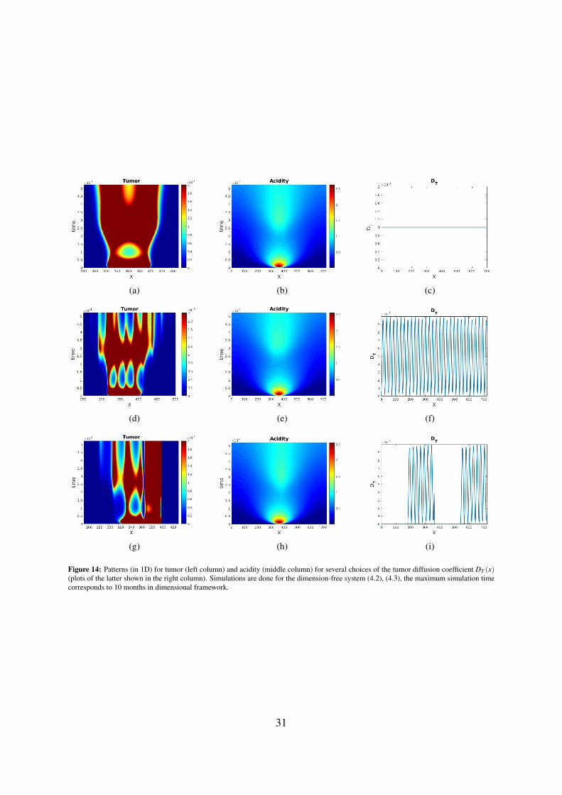
Figure 14: Patterns (in 1D) for tumor (left column) and acidity (middle column) for several choices of the tumor diffusion coefficient DT (x)(plots of the latter shown in the right column). Simulations are done for the dimension-free system (4.2), (4.3), the maximum simulation timecorresponds to 10 months in dimensional framework.

31

does not seem to be appropriate for describing pseudopalisade formation.

The above suggests that pseudopalisades are not Turing-like patterns - at least as far as our model withconstant diffusion coefficient is used for their description. To see the effect of the diffusion coefficientDT (x) we plot in Figure 14 the patterns obtained in 1D for the same parameter combination and severalchoices of DT (x), including various kinds of degeneracy. Thus, the second row in Figure 14 shows thecase where DT degenerates on countable set, while the last row illustrates the situation with a strongdegeneracy, i.e. on whole subintervals of the space domain (DT is of the type considered in [60] for aclosely related problem, however with haptotaxis).

References

[1] J.C.L. Alfonso, A. Kohn-Luque, T. Stylianopoulos, F. Feuerhake, A. Deutsch, and H. Hatzikirou.Why one-size-fits-all vaso-modulatory interventions fail to control glioma invasion: in silicoinsights. Scientific Reports, 6:37283, 2016.

[2] S. Banerjee, S. Khajanchi, and S. Chaudhuri. A mathematical model to elucidate brain tumorabrogation by immunotherapy with t11 target structure. PLOS ONE, 10(5):e0123611, 2015.

[3] P. Bartel, F.T. Ludwig, A. Schwab, and C. Stock. pH-taxis: Directional tumor cell migration alongpH-gradients. Acta Physiologica, 204, Suppl. 689:113, 2012.

[4] N. Bellomo. Modeling Complex Living Systems. Birkhauser Boston, 2008.

[5] K. Bottger, H. Hatzikirou, A. Chauviere, and A. Deutsch. Investigation of themigration/proliferation dichotomy and its impact on avascular glioma invasion. Math. Model Nat.Phenom., 7:105–135, 2012.

[6] N.H. Boyd, K. Walker, J. Fried, J.R. Hackney, P.C. McDonald, G.A. Benavides, R. Spina,A. Audia, S.E. Scott, C.J. Libby, A.N. Tran, M.O. Bevensee, C. Griguer, S. Nozell, G.Y. Gillespie,B. Nabors, K.P. Bhat, E.E. Bar, V. Darley-Usmar, B. Xu, E. Gordon, S.J. Cooper, S. Dedhar,and A.B. Hjelmeland. Addition of carbonic anhydrase 9 inhibitor SLC-0111 to temozolomidetreatment delays glioblastoma growth in vivo. JCI Insight, 2(24), December 2017.

[7] D.J. Brat, A. Castellano-Sanchez, B. Kaur, and E.G. Van Meir. Genetic and biologic progressionin astrocytomas and their relation to angiogenic dysregulation. Advances in Anatomic Pathology,9(1):24–36, 2002.

[8] D.J. Brat, A.A. Castellano-Sanchez, S.B. Hunter, M. Pecot, C. Cohen, E.H. Hammond, S.N. Devi,B. Kaur, and E.G. Van Meir. Pseudopalisades in glioblastoma are hypoxic, express extracellularmatrix proteases, and are formed by an actively migrating cell population. Cancer Research,64(3):920–927, 2004.

[9] D.J. Brat and T.B. Mapstone. Malignant glioma physiology: cellular response to hypoxia and itsrole in tumor progression. Annals of Internal Medicine, 138(8):659–668, 2003.

[10] D.J. Brat and E.G. Van Meir. Vaso-occlusive and prothrombotic mechanisms associated with tumorhypoxia, necrosis, and accelerated growth in glioblastoma. Laboratory Investigation, 84(4):397–405, 2004.

[11] Y. Cai, J. Wu, Z. Li, and Q. Long. Mathematical modelling of a brain tumour initiation and earlydevelopment: a coupled model of glioblastoma growth, pre-existing vessel co-option, angiogenesisand blood perfusion. PloS one, 11(3):e0150296, 2016.

32

[12] A. Caiazzo and I. Ramis-Conde. Multiscale modelling of palisade formation in gliobastomamultiforme. Journal of theoretical biology, 383:145–156, 2015.

[13] X. Cao. Boundedness in a quasilinear parabolic–parabolic keller–segel system with logistic source.Journal of Mathematical Analysis and Applications, 412(1):181–188, 2014.

[14] G. Corbin, C. Engwer, A. Klar, J. Nieto, J. Soler, C. Surulescu, and M. Wenske. On a model forglioma invasion with anisotropy- and hypoxia-triggered motility enhancement: from subcellulardynamics to nonlocal macroscopic PDEs with multiple taxis. arXiv:2006.12322.

[15] G. Corbin, A. Hunt, A. Klar, F. Schneider, and C. Surulescu. Higher-order models for gliomainvasion: From a two-scale description to effective equations for mass density and momentum.Mathematical Models and Methods in Applied Sciences, 28(09):1771–1800, 2018.

[16] S.E. Eikenberry, T. Sankar, M.C. Preul, E.J. Kostelich, C.J. Thalhauser, and Y. Kuang. Virtualglioblastoma: growth, migration and treatment in a three-dimensional mathematical model. CellProliferation, 42(4):511–528, 2009.

[17] C. Engwer, T. Hillen, M. Knappitsch, and C. Surulescu. Glioma follow white matter tracts: amultiscale DTI-based model. Journal of Mathematical Biology, 71(3):551–582, 2015.

[18] C. Engwer, A. Hunt, and C. Surulescu. Effective equations for anisotropic glioma spread withproliferation: a multiscale approach and comparisons with previous settings. MathematicalMedicine and Biology: an IMA Journal, 33(4):435–459, 2015.

[19] C. Engwer, M. Knappitsch, and C. Surulescu. A multiscale model for glioma spread includingcell-tissue interactions and proliferation. J. Math. Biosc. Eng., 13:443–460, 2016.

[20] I. Fischer, J.-P. Gagner, M. Law, E.W. Newcomb, and D. Zagzag. Angiogenesis in gliomas:Biology and molecular pathophysiology. Brain Pathology, 15(4):297–310, 2006.

[21] R.A. Gatenby and E.T. Gawlinski. A reaction-diffusion model of cancer invasion. CancerResearch, 56(24):5745–5753, 1996.

[22] L. Hathout, B.M. Ellingson, T. Cloughesy, and W.B. Pope. A novel bicompartmental mathematicalmodel of glioblastoma multiforme. International Journal of Oncology, 46(2):825–832, 2014.

[23] T. Hillen. M5 mesoscopic and macroscopic models for mesenchymal motion. J. Math. Biol., 53,2006.

[24] T. Hillen and K.J. Painter. Transport and anisotropic diffusion models for movement in orientedhabitats. In Dispersal, individual movement and spatial ecology, pages 177–222. Springer, 2013.

[25] S. Hiremath and C. Surulescu. A stochastic multiscale model for acid mediated cancer invasion.Nonlinear Analysis: Real World Applications, 22:176–205, 2015.

[26] S. Hiremath and C. Surulescu. A stochastic model featuring acid-induced gaps during tumorprogression. Nonlinearity, 29(3):851–914, 2016.

[27] S. Hiremath, C. Surulescu, A. Zhigun, and S. Sonner. On a coupled SDE-PDE system modelingacid-mediated tumor invasion. Discrete & Continuous Dynamical Systems - B, 23(6):2339–2369,2018.

[28] P. Holzer. Acid-sensitive ion channels and receptors. In Sensory Nerves, pages 283–332. SpringerBerlin Heidelberg, 2009.

33

[29] A. Hunt and C. Surulescu. A multiscale modeling approach to glioma invasion with therapy.Vietnam Journal of Mathematics, 45(1-2):221–240, 2016.

[30] J. Kelkel and C. Surulescu. On some models for cancer cell migration through tissue networks.Mathematical Biosciences and Engineering, 8(2):575–589, 2011.

[31] J. Kelkel and C. Surulescu. A multiscale approach to cell migration in tissue networks.Mathematical Models and Methods in Applied Sciences, 22(03):1150017, 2012.

[32] E. Khain, M. Katakowski, S. Hopkins, A. Szalad, X. Zheng, F. Jiang, and M. Chopp. Collectivebehavior of brain tumor cells: The role of hypoxia. Phys. Rev. E, 83:031920, 2011.

[33] P. Kleihues, F. Soylemezoglu, B. Schauble, B.W. Scheithauer, and P.C. Burger. Histopathology,classification and grading of gliomas. Glia, 5:211–221, 1995.

[34] P.E. Kloeden, S. Sonner, and C. Surulescu. A nonlocal sample dependence SDE-PDE systemmodeling proton dynamics in a tumor. Discrete and Continuous Dynamical Systems - Series B,21(7):2233–2254, 2016.

[35] T. Koltai, S.J. Reshkin, and S. Harguindey. The pH-centered paradigm in cancer. In An InnovativeApproach to Understanding and Treating Cancer: Targeting pH, pages 53–97. Elsevier, 2020.

[36] D.A. Lauffenburger and J.L. Lindermann. Receptors. Models for binding, trafficing and signaling.Oxford University Press, 1993.

[37] T. Lorenz and C. Surulescu. On a class of multiscale cancer cell migration models: Well-posedness in less regular function spaces. Mathematical Models and Methods in Applied Sciences,24(12):2383–2436, 2014.

[38] D.N. Louis, H. Ohgaki, O.D. Wiestler, W.K. Cavenee, P.C. Burger, A. Jouvet, B.W. Scheithauer,and P. Kleihues. The 2007 WHO classification of tumours of the central nervous system. ActaNeuropathologica, 114(2):97–109, 2007.

[39] N. Loy and L. Preziosi. Kinetic models with non-local sensing determining cell polarization andspeed according to independent cues. Journal of Mathematical Biology, 80:374–421, 2020.

[40] G.R. Martin and R.K. Jain. Noninvasive measurement of interstitial pH profiles in normal andneoplastic tissue using fluorescence ratio imaging microscopy. Cancer Research, 54(21):5670–5674, 1994.

[41] A. Martınez-Gonzalez, G.F. Calvo, L.A. Perez Romasanta, and V.M. Perez-Garcıa. Hypoxiccell waves around necrotic cores in glioblastoma: a biomathematical model and its therapeuticimplications. Bulletin of Mathematical Biology, 74(12):2875–2896, 2012.

[42] A. McIntyre, S. Patiar, S. Wigfield, J. l. Li, I. Ledaki, H. Turley, R. Leek, C. Snell, K. Gatter,W. S. Sly, R. D. Vaughan-Jones, P. Swietach, and A. L. Harris. Carbonic anhydrase IX promotestumor growth and necrosis in vivo and inhibition enhances anti-VEGF therapy. Clinical CancerResearch, 18(11):3100–3111, 2012.

[43] P. Mosayebi, D. Cobzas, M. Jagersand, and A. Murtha. Stability effects of finite difference methodson a mathematical tumor growth model. In 2010 IEEE Computer Society Conference on ComputerVision and Pattern Recognition-Workshops, pages 125–132. IEEE, 2010.

[44] H.G. Othmer and T. Hillen. The diffusion limit of transport equations II: Chemotaxis equations.SIAM Journal on Applied Mathematics, 62(4):1222–1250, 2002.

34

[45] K. Painter and T. Hillen. Mathematical modelling of glioma growth: the use of diffusion tensorimaging (DTI) data to predict the anisotropic pathways of cancer invasion. J. Theor. Biol. 323,pages pp. 25–39, 2013.

[46] R.K. Paradise, M.J. Whitfield, D.A. Lauffenburger, and K.J. Van Vliet. Directional cell migrationin an extracellular pH gradient: A model study with an engineered cell line and primarymicrovascular endothelial cells. Experimental Cell Research, 319(4):487–497, 2013.

[47] B. Perthame, M. Tang, and N. Vauchelet. Derivation of the bacterial run-and-tumble kineticequation from a model with biochemical pathway. Journal of Mathematical Biology, 73(5):1161–1178, 2016.

[48] S. Prag, E.A. Lepekhin, K. Kolkova, R. Hartmann-Petersen, A. Kawa, P.S. Walmod, V. Belman,H.C. Gallagher, V. Berezin, E. Bock, and N. Pedersen. Ncam regulates cell motility. Journal ofCell Science, 115(2):283–292, 2002.

[49] D. Ramnani. WebPathology - visual survey of surgical pathology. https://www.webpathology.com.

[50] R. Rockne, J.K. Rockhill, M. Mrugala, A.M. Spence, I. Kalet, K. Hendrickson, A. Lai,T. Cloughesy, E.C. Alvord, and K.R. Swanson. Predicting the efficacy of radiotherapy in individualglioblastoma patients in vivo:a mathematical modeling approach. Physics in Medicine and Biology,55(12):3271–3285, 2010.

[51] Y. Rong, D.L. Durden, E.G. Van Meir, and D.J. Brat. ‘Pseudopalisading’necrosis in glioblastoma:a familiar morphologic feature that links vascular pathology, hypoxia, and angiogenesis. Journalof Neuropathology & Experimental Neurology, 65(6):529–539, 2006.

[52] L.M Sander and T.S Deisboeck. Growth patterns of microscopic brain tumors. Physical Review E,66(5):051901, 2002.

[53] P.A. Schornack and R.J. Gillies. Contributions of cell metabolism and H+ diffusion to the acidicpH of tumors. Neoplasia (New York, NY), 5(2):135, 2003.

[54] M. Sidani, D. Wessels, G. Mouneimne, M. Ghosh, S. Goswami, C. Sarmiento, W. Wang, S. Kuhl,M. El-Sibai, J.M. Backer, et al. Cofilin determines the migration behavior and turning frequencyof metastatic cancer cells. The Journal of Cell Biology, 179(4):777–791, 2007.

[55] A.M. Stein, T. Demuth, D. Mobley, M. Berens, and L.M. Sander. A mathematical model ofglioblastoma tumor spheroid invasion in a three-dimensional in vitro experiment. BiophysicalJournal, 92(1):356–365, 2007.

[56] Y. Tao and M. Winkler. Large time behavior in a multidimensional chemotaxis-haptotaxis modelwith slow signal diffusion. SIAM Journal on Mathematical Analysis, 47(6):4229–4250, 2015.

[57] B.A. Webb, M. Chimenti, M.P. Jacobson, and D.L. Barber. Dysregulated pH: a perfect storm forcancer progression. Nature Reviews Cancer, 11(9):671–677, 2011.

[58] J. Weickert. Anisotropic diffusion in image processing, volume 1. Teubner Stuttgart, 1998.

[59] M. Winkler. Global solutions in a fully parabolic chemotaxis system with singular sensitivity.Mathematical Methods in the Applied Sciences, 34(2):176–190, 2010.

[60] M. Winkler and C. Surulescu. Global weak solutions to a strongly degenerate haptotaxis model.Communications in Mathematical Sciences, 15(6):1581–1616, 2017.

35

[61] F.J. Wippold, M. Lammle, F. Anatelli, J. Lennerz, and A. Perry. Neuropathology forthe neuroradiologist: palisades and pseudopalisades. American Journal of Neuroradiology,27(10):2037–2041, 2006.

[62] M. Wrensch, Y. Minn, T. Chew, M. Bondy, and M.S. Berger. Epidemiology of primary braintumors: Current concepts and review of the literature. Neuro-Oncology, 4:278–299, 2002.

36