
Multiprocessor Scheduling
447
Multiprocessor Scheduling Theory and Applications
-
Upload
usmaniyusuf -
Category
Documents
-
view
570 -
download
13
Transcript of Multiprocessor Scheduling

Multiprocessor Scheduling Theory and Applications


Multiprocessor Scheduling Theory and Applications
Edited by Eugene Levner
I-TECH Education and Publishing

Published by the I-Tech Education and Publishing, Vienna, Austria
Abstracting and non-profit use of the material is permitted with credit to the source. Statements and opinions expressed in the chapters are these of the individual contributors and not necessarily those of the editors or publisher. No responsibility is accepted for the accuracy of information contained in the published articles. Publisher assumes no responsibility liability for any damage or injury to persons or property arising out of the use of any materials, instructions, methods or ideas contained inside. After this work has been published by the I-Tech Education and Publishing, authors have the right to republish it, in whole or part, in any publication of which they are an author or editor, and the make other personal use of the work.
© 2007 I-Tech Education and Publishing www.i-techonline.com Additional copies can be obtained from: [email protected]
First published December 2007 Printed in Croatia
A catalogue record for this book is available from the Austrian Library. Multiprocessor Scheduling: Theory and Applications, Edited by Eugene Levner
p. cm. ISBN 978-3-902613-02-8
1. Scheduling. 2. Theory and Applications. 3. Levner.

V
Preface
Scheduling theory is concerned with the optimal allocation of scarce resources (for instance, machines, processors, robots, operators, etc.) to activities over time, with the objective of optimizing one or several performance measures. The study of scheduling started about fifty years ago, being initiated by seminal papers by Johnson (1954) and Bellman (1956). Since then machine scheduling theory have received considerable development. As a result, a great diversity of scheduling models and optimization techniques have been developed that found wide applications in industry, transport and communications. Today, scheduling theory is an integral, generally recognized and rapidly evolving branch of operations research, fruitfully contributing to computer science, artificial intelligence, and industrial engineering and management. The interested reader can find many nice pearls of scheduling theory in textbooks, monographs and handbooks by Tanaev et al. (1994a,b), Pinedo (2001), Leung (2001), Brucker (2007), and Blazewicz et al. (2007). This book is the result of an initiative launched by Prof. Vedran Kordic, a major goal of which is to continue a good tradition - to bring together reputable researchers from different countries in order to provide a comprehensive coverage of advanced and modern topics in scheduling not yet reflected by other books. The virtual consortium of the authors has been created by using electronic exchanges; it comprises 50 authors from 18 different countries who have submitted 23 contributions to this collective product. In this sense, the volume in your hands can be added to a bookshelf with similar collective publications in scheduling, started by Coffman (1976) and successfully continued by Chretienne et al. (1995), Gutin and Punnen (2002), and Leung (2004). This volume contains four major parts that cover the following directions: the state of the art in theory and algorithms for classical and non-standard scheduling problems; new exact optimization algorithms, approximation algorithms with performance guarantees, heuristics and metaheuristics; novel models and approaches to scheduling; and, last but least, several real-life applications and case studies. The brief outline of the volume is as follows. Part I presents tutorials, surveys and comparative studies of several new trends and modern tools in scheduling theory. Chapter 1 is a tutorial on theory of cyclic scheduling. It is included for those readers who are unfamiliar with this area of scheduling theory. Cyclic scheduling models are traditionally used to control repetitive industrial processes and enhance the performance of robotic lines in many industries. A brief overview of cyclic scheduling models arising in manufacturing systems served by robots is presented, started with a discussion of early works appeared in the 1960s. Although the considered scheduling problems are, in general, NP-hard, a graph approach presented in this chapter permits to reduce some special cases to the parametric critical path problem in a graph and solve them in polynomial time. Chapter 2 describes the so-called multi-agent scheduling models applied to the situations in which the resource allocation process involves different stakeholders (“agents”), each having his/her own set of jobs and interests, and there is no central authority which can

VI
solve possible conflicts in resource usage over time. In this case, standard scheduling models become invalid, since rather than computing "optimal solutions”, the model is asked to provide useful elements for the negotiation process, which eventually should lead to a stable and acceptable resource allocation. The chapter does not review the whole scope in detail, but rather concentrates on combinatorial models and their applications. Two major mechanisms for generating schedules, auctions and bargaining models, corresponding to different information exchange scenarios, are considered. Known results are reviewed and venues for future research are pointed out. Chapter 3 considers a class of scheduling problems under unavailability constraints associated, for example, with breakdown periods, maintenance durations and/or setup times. Such problems can be met in different industrial environments in numerous real-life applications. Recent algorithmic approaches proposed to solve these problems are presented, and their complexity and worst-case performance characteristics are discussed. The main attention is devoted to the flow-time minimization in the weighted and unweighted cases, for single-machine and parallel machine scheduling problems. Chapter 4 is devoted to the analysis of scheduling problems with communication delays. With the increasing importance of parallel computing, the question of how to schedule a set of precedence-constrained tasks on a given computer architecture, with communication delays taken into account, becomes critical. The chapter presents the principal results related to complexity, approximability and non-approximability of scheduling problems in presence of communication delays. Part II comprising eight chapters is devoted to the design of scheduling algorithms. Here the reader can find a wide variety of algorithms: exact, approximate with performance guarantees, heuristics and meta-heuristics; most algorithms are supplied by the complexity analysis and/or tested computationally. Chapter 5 deals with a batch version of the single-processor scheduling problem with batch setup times and batch delivery costs, the objective being to find a schedule which minimizes the sum of the weighted number of late jobs and the delivery costs. A new dynamic programming (DP) algorithm which runs in pseudo-polynomial time is proposed. By combining the techniques of binary range search and static interval partitioning, the DP algorithm is converted into a fully polynomial time approximation scheme for the general case. The DP algorithm becomes polynomial for the special cases when jobs have equal weights or equal processing times. Chapter 6 studies on-line approximation algorithms with performance guarantees for an important class of scheduling problems defined on identical machines, for jobs with arbitrary release times. Chapter 7 presents a new hybrid metaheuristic for solving the jobshop scheduling problem that combines augmented-neural-networks with genetic algorithm based search. In Chapter 8 heuristics based on a combination of the guided search and tabu search are considered to minimize the maximum completion time and maximum tardiness in the parallel-machine scheduling problems. Computational characteristics of the proposed heuristics are evaluated through extensive experiments. Chapter 9 presents a hybrid meta-heuristics based on a combination of the genetic algorithm and the local search aimed to solve the re-entrant flowshop scheduling problems. The hybrid method is compared with the optimal solutions generated by the integer programming technique, and the near optimal solutions generated by a pure genetic algorithm. Computational experiments are performed to illustrate the effectiveness and efficiency of the proposed algorithm.

VII
Chapter 10 is devoted to the design of different hybrid heuristics to schedule a bottleneck machine in a flexible manufacturing system problems with the objective to minimize the total weighted tardiness. Search algorithms based on heuristic improvement and local evolutionary procedures are formulated and computationally compared. Chapter 11 deals with a multi-objective no-wait flow shop scheduling problem in which the weighted mean completion time and the weighted mean tardiness are to be optimized simultaneously. To tackle this problem, a novel computational technique, inspired by immunology, has emerged, known as artificial immune systems. An effective multi-objective immune algorithm is designed for searching the Pareto-optimal frontier. In order to validate the proposed algorithm, various test problems are designed and the algorithm is compared with a conventional multi-objective genetic algorithm. Comparison metrics, such as the number of Pareto optimal solutions found by the algorithm, error ratio, generational distance, spacing metric, and diversity metric, are applied to validate the algorithm efficiency. The experimental results indicated that the proposed algorithm outperforms the conventional genetic algorithm, especially for the large-sized problems. Chapter 12 considers a version of the open-shop problem called the concurrent open shop with the objective of minimizing the weighted number of tardy jobs. A branch and bound algorithm is developed. Then, in order to produce approximate solutions in a reasonable time, a heuristic and a tabu search algorithm are proposed.. Computational experiments support the validity and efficiency of the tabu search algorithm. Part III comprises seven chapters and deals with new models and decision making approaches to scheduling. Chapter 13 addresses an integrative view for the production scheduling problem, namely resources integration, cost elements integration and solution methodologies integration. Among methodologies considered and being integrated together are mathematical programming, constraint programming and metaheuristics. Widely used models and representations for production scheduling problems are reconsidered, and optimization objectives are reviewed. An integration scheme is proposed and performance of approaches is analyzed. Chapter 14 examines scheduling problems confronted by planners in multi product chemical plants that involve sequencing of jobs with sequence-dependent setup time. Two mixed integer programming (MIP) formulations are suggested, the first one aimed to minimize the total tardiness while the second minimizing the sum of total earliness/tardiness for parallel machine problem. Chapter 15 presents a novel mixed-integer programming model of the flexible flow line problem that minimizes the makespan. The proposed model considers two main constraints, namely blocking processors and sequence-dependent setup time between jobs. Chapter 16 considers the so-called hybrid jobshop problem which is a combination of the standard jobshop and parallel machine scheduling problems with the objective of minimizing the total tardiness. The problem has real-life applications in the semiconductor manufacturing or in the paper industries. Efficient heuristic methods to solve the problem, namely, genetic algorithms and ant colony heuristics, are discussed. Chapter 17 develops the methodology of dynamical gradient Artificial Neural Networks for solving the identical parallel machine scheduling problem with the makespan criterion (which is known to be NP-hard even for the case of two identical parallel machines). A Hopfield-like network is proposed that uses time-varying penalty parameters. A novel time-varying penalty method that guarantees feasible and near optimal solutions for solving the problem is suggested and compared computationally with the known LPT heuristic.

VIII
In Chapter 18 a dynamic heuristic rule-based approach is proposed to solve the resource constrained scheduling problem in an FMS, and to determine the best routes of the parts, which have routing flexibility. The performance of the proposed rule-based system is compared with single dispatching rules. Chapter 19 develops a geometric approach to modeling a large class of multithreaded programs sharing resources and to scheduling concurrent real-time processes. This chapter demonstrates a non-trivial interplay between geometric approaches and real-time programming. An experimental implementation allowed to validate the method and provided encouraging results. Part IV comprises four chapters and introduces real-life applications of scheduling theory and case studies in the sheet metal shop (Chapter 20), baggage handling systems (Chapter 21), large-scale supply chains (Chapter 22), and semiconductor manufacturing and photolithography systems (Chapter 23). Summing up the wide range of issues presented in the book, it can be addressed to a quite broad audience, including both academic researchers and practitioners in halls of industries interested in scheduling theory and its applications. Also, it is heartily recommended to graduate and PhD students in operations research, management science, business administration, computer science/engineering, industrial engineering and management, information systems, and applied mathematics. This book is the result of many collaborating parties. I gratefully acknowledge the assistance provided by Dr. Vedran Kordic, Editor-in-Chief of the book series, who initiated this project, and thank all the authors who contributed to the volume.
References Bellman, R., (1956). Mathematical aspects of scheduling theory. Journal of Society of Industrial
and Applied Mathematics 4, 168–205. Blazewicz, J., Ecker, K.H., Pesch, E., Schmidt, G., and Weglarz (2007), Handbook on Scheduling,
From Theory to Applications, Springer. Berlin. Brucker, P. (2007), Scheduling Algorithms, Springer, 5th edition, Berlin. Chretienne, P., Coffman, E.G., Lenstra, J.K., Liu, Z. (eds.) (1995), Scheduling Theory and its
Applications, Wiley, New York. Coffman, E.G., Jr. (ed.), (1976), Scheduling in Computer and Job Shop Systems, Wiley, New York. Gutin, G. and Punnen, A.P. (eds.) (2002), The Traveling Salesman Problem and Its Variations,
Springer, Berlin, 848 p. Johnson, S.M. (1954). Optimal two- and three-stage production schedules with setup times
included. Naval Research Logistics Quarterly 1, 61–68. Lawler, E., Lenstra, J., Rinnooy Kan, A., and Shmoys, D. (1985) The Traveling Salesman Problem:
A Guided Tour of Combinatorial Optimization, Wiley, New York. Leung, J.Y.-T. (ed.) (2004), Handbook of Scheduling: Algorithms, Models, and Performance
Analysis, Chapman & Hall/CRC, Boca Raton Pinedo, M. (2001), Scheduling: Theory, Algorithms and Systems, Prentice Hall, Englewood Cliffs. Tanaev, V.S., Gordon, V.S., and Shafransky, Ya.M. (1994), Scheduling Theory. Single-Stage
Systems, Kluwer, Dordrecht. Tanaev, V.S., Sotskov,Y.N. and Strusevich, V.A.. (1994), Scheduling Theory. Multi-Stage Systems,
Kluwer, Dordrecht.
Eugene Levner September 10,2007

IX
Contents
Preface ........................................................................................................................................V
Part I. New Trends and Tools in Scheduling: Surveys and Analysis
1. Cyclic Scheduling in Robotic Cells: An Extension of Basic Models in Machine Scheduling Theory ....................................001Eugene Levner, Vladimir Kats and David Alcaide Lopez De Pablo
2. Combinatorial Models for Multi-agent Scheduling Problems ...................................021Alessandro Agnetis, Dario Pacciarelli and Andrea Pacifici
3. Scheduling under Unavailability Constraints to Minimize Flow-time Criteria ........047Imed Kacem
4. Scheduling with Communication Delays ......................................................................063R. Giroudeau and J.C. Kinig
Part II. Exact Algorithms, Heuristics and Complexity Analysis
5. Minimizing the Weighted Number of Late Jobs with Batch Setup Times and Delivery Costs on a Single Machine ............085George Steiner and Rui Zhang
6. On-line Scheduling on Identical Machines for Jobs with Arbitrary Release Times ...........................................099Li Rongheng and Huang Huei-Chuen
7. A NeuroGenetic Approach for Multiprocessor Scheduling .......................................121Anurag Agarwal
8. Heuristics for Unrelated Parallel Machine Scheduling with Secondary Resource Constraints ........................................................137Jeng-Fung Chen

X
9. A hybrid Genetic Algorithm for the Re-entrant Flow-shop Scheduling Problem .........................................................153Jen-Shiang Chen, Jason Chao-Hsien Pan and Chien-Min Lin
10. Hybrid Search Heuristics to Schedule Bottleneck Facility in Manufacturing Systems ..........................................167Ponnambalam S.G., Jawahar.N and Maheswaran. R
11. Solving a Multi-Objective No-Wait Flow Shop Problem by a Hybrid Multi-Objective Immune Algorithm ....................................195R. Tavakkoli-Moghaddam, A. Rahimi-Vahed and A. Hossein Mirzaei
12. Concurrent Openshop Problem to Minimize the Weighted Number of Late Jobs ..............................................................215H.L. Huang and B.M.T. Lin
Part III. New Models and Decision Making Approaches
13. Integral Approaches to Integrated Scheduling .........................................................221Ghada A. El Khayat
14. Scheduling with setup Considerations: An MIP Approach .....................................241Mohamed. K. Omar, Siew C. Teo and Yasothei Suppiah
15. A New Mathematical Model for Flexible Flow Lines with Blocking Processor and Sequence-Dependent Setup Time ......................255R. Tavakkoli-Moghaddam and N. Safaei
16. Hybrid Job Shop and Parallel Machine Scheduling Problems: Minimization of Total Tardiness Criterion ................................273Frederic Dugardin, Hicham Chehade, Lionel Amodeo, Farouk Yalaoui and Christian Prins
17. Identical Parallel Machine Scheduling with Dynamical Networks using Time-Varying Penalty Parameters .....................................293Derya Eren Akyol
18. A Heuristic Rule-Based Approach for Dynamic Scheduling of Flexible Manufacturing Systems .............................................315Gonca Tuncel
19. A Geometric Approach to Scheduling of Concurrent Real-time Processes Sharing Resources ...............................................323Thao Dang and Philippe Gerner

XI
Part IV. Real-Life Applications and Case Studies
20. Sequencing and Scheduling in the Sheet Metal Shop ..................................................345B. Verlinden, D. Cattrysse, H. Crauwels, J. Duflou and D. Van Oudheusden
21. Decentralized Scheduling of Baggage Handling using Multi Agent Technologies .......................................................381Kasper Hallenborg
22. Synchronized Scheduling of Manufacturing and 3PL Transportation ...................405Kunpeng Li and Appa Iyer Sivakumar
23. Scheduling for Dedicated Machine Constraint ..........................................................417Arthur Shr, Peter P. Chen and Alan Liu

1
Cyclic Scheduling in Robotic Cells: An Extension of Basic Models in Machine
Scheduling Theory
Eugene Levner1, Vladimir Kats2 and David Alcaide López De Pablo3
1Holon Institute of Technology, Holon, 2Institute of Industrial Mathematics, Beer-Sheva, 3University of La Laguna, La Laguna, Tenerife
1, 2 Israel, 3Spain
1. Introduction
There is a growing interest on cyclic scheduling problems both in the scheduling literature and among practitioners in the industrial world. There are numerous examples of applications of cyclic scheduling problems in different industries (see, e.g., Hall (1999), Pinedo (2001)), automatic control (Romanovskii (1967), Cohen et al. (1985)), multi-processor computations (Hanen and Munier (1995), Kats and Levner (2003)), robotics (Livshits et al. (1974), Kats and Mikhailetskii (1980), Kats (1982), Sethi et al. (1992), Lei (1993), Kats and Levner (1997a, 1997b), Hall (1999), Crama et al. (2000), Agnetis and Pacciarelli (2000), Dawande et al. (2005, 2007)), and in communications and transport (Dauscha et al. (1985), Sharma and Paradkar (1995), Kubiak (2005)). It is, perhaps, a surprising thing that many facts in scheduling theory obtained as early as in the 1960s, are re-discovered and re-rediscovered by the next generations of researchers. About two decades ago, this fact was noticed by Serafini and Ukovich (1989). The present survey uniformly addresses cyclic scheduling problems through the prism of the classical machine scheduling theory focusing on their features that are common for all aforementioned applications. Historically, the scheduling literature considered periodic machine scheduling problems in two major classes – called flowshop and jobshop - in which setup and transportation times were assumed insignificant. Indeed, many machining centers can quickly switch tools, so the setup times for these situations may be small or negligible. There are a lot of results about cyclic flowshop and jobshop problems with negligible setup/transportation times. Advantages of cyclic scheduling policies over conventional (non-cyclic) scheduling in flexible manufacturing are widely discussed in the literature, we refer the interested reader to Karabati and Kouvelis (1996), Lee and Posner (1997), Hall et al. (2002), Seo and Lee (2002), Timkovsky (2004), Dawande et al. (2007), and numerous references therein. At the same time, modern flexible manufacturing systems are supplied by computer-controlled hoists, robots and other material handling devices such that the transportation and setup operation times are significant and should not be ignored. Robots have become a standard tool to serve cyclic transportation and assembling/disassembling processes in manufacturing of airplanes, automobiles, semiconductors, printed circuit boards, food

Multiprocessor Scheduling: Theory and Applications 2
products, pharmaceutics and cosmetics. Robots have expanded production capabilities in the manufacturing world making the assembly process faster, more efficient and precise than ever before. Robots save workers from tedious and dull assembly line jobs, and increase production and savings in the processes. As larger and more complex robotic cells are implemented, more sophisticated planning and scheduling models and algorithms are required to perform and optimize these processes. The cyclic scheduling problems, in which setup operations are performed by automatic transporting devices, constitute a vast subclass of cyclic problems. Robots or other automatic devices are explicitly introduced into the models and treated as special purpose machines. In this chapter, we will focus on three major classes of cyclic scheduling problems – flowshop, jobshop, and parallel machine shop.The chapter is structured as follows. Section 2 is a historical overview, with the main attention being paid to the early works of the 1960s. Section 3 recalls three orthodox classes of scheduling theory: flowshop, jobshop, and PERT-shop. Each of these classes can be extended in two directions: (a) for describing periodic processes with negligible setups, and (b) for describing periodic processes in robotic cells where setups and transportation times are non-negligible. In Section 4 we consider an extension of the cyclic PERT-shop, called the cyclic FMS-shop and demonstrate that its important special case can be solved efficiently by using a graph approach. Section 5 concludes the chapter.
2. Brief Historical Overview
Cyclic scheduling problems have been introduced in the scheduling literature in the early 1960s, some of them assuming setup/transportation times negligible while other explicitly treating material handling devices with non-negligible operation times. Cyclic Flowshop. Cuninghame-Greene (1960, 1962) has described periodic industrial processes, which in today’s terminology might be classified as a cyclic flowshop (without setups and robots), and suggested an algebraic method for finding minimum cycle time using matrix multiplication in which one writes “addition” in place of multiplication and operation “max” instead of addition. This (max, +)–algebra has become popular in the 1980s (see, e.g. Cuninghame-Greene (1979), Cohen et al. (1985), Baccelli et al. (1992)) and is presently used for solving the cyclic flowshop without robots, see, e.g., Hanen (1994), Hanen and Munier (1995), Lee (2000), and Seo and Lee (2002). Independently of the latter research, Degtyarev and Timkovsky (1976) and Timkovsky (1977) have studied so-called spyral cyclograms widely used in the Soviet electronic industry; they introduced a generalized shop structure which they called a “cycle shop”. Using a more standard terminology, we might say that these authors have been the first to study aflowshop with reentrant machines which includes, as special cases, many variants of the basic flowshop, for instance, the reentrant flowshop of Graves et al. (1983), V-shop of Lev and Adiri (1984), cyclic robotic flowshop of Kats and Levner (1997, 1998, 2002). The interested reader is referred to Middendorf and Timkovsky (2002) and Timkovsky (2004) for more details. Cyclic Robotic Flowshop. In the beginning of 1960s, a group of Byelorussian mathematicians (Suprunenko et al. (1962), Aizenshtat (1963), Tanaev (1964), and others) investigated cyclic processes in manufacturing lines served by transporting devices. The latters differ from other machines in their physical characteristics and functioning. These authors have introduced a cyclic robotic flowshop problem and suggested, in particular, a combinatorial

Cyclic Scheduling in Robotic Cells: The Extension of Basic Models in Machine Scheduling Theory 3
method called the method of forbidden intervals which today is being developed further by different authors for various cyclic robotic scheduling problems (see, for example, Livshits et al. (1974), Levner et al. (1997), Kats et al. (1999), Che and Chu (2005a, 2005b), Chu (2006), Che et al. (2002, 2003)). A thorough review in this area can be found in the surveys by Hall (1999), Crama et al. (2000), Manier and Bloch (2003), and Dawande et al. (2005, 2007). Cyclic PERT-shop. The following cyclic PERT-shop problem has originated in the work by Romanovskii (1967). There is a set S of n partially ordered operations, called generic operations, to be processed on machines. As in the classic (non-cyclic) PERT/CPM problem, each operation is done by a dedicated machine and there is sufficiently many machines to perform all operations; so the question of scheduling operations on machines vanishes. Each operation i has processing time pi > 0 and must be performed periodically with the same period T, infinitely many times. For each operation i, let <i, k> denote the kth execution (or, repetition) of operation i in a schedule (here k is any positive integer). Precedence relations are defined as follows (here we use a slightly different notation than that given by Romanovskii). If a generic operation iprecedes a generic operation j, the corresponding edge (i, j) is introduced. Any edge (i,j) is supplied by two given values, Lij called the length, or delay, and Hij called the height of the corresponding edge (i, j). The former value is any rational number of any sign while the latter is integer. Then, for a pair of operations i and j, and the given length Lij and height Hij,
the following relations are given: for all k 1, t(i,k) + Lij t(j, k + Hij), where t(i,k) is the starting time of operation <i, k>. An edge is called interior if its end-nodes belong to the same iteration (or, one can say “to the same block, or pattern”) and backward (or, recycling) if its end-nodes belong to two consecutive blocks. A schedule is called periodic (or cyclic) with cycle time T if t(i, k) = t(i,1) + (k-1)T, for all
integer k 1, and for all i S (see Fig. 1). The problem is to find a periodic schedule (i.e., the starting time t(i,1) of operations) providing a minimum cycle time T, in a graph with the infinite number of edges representing an infinitely repeating process.
Figure 1. The cyclic PERT graph (from Romanovskii, (1967))
In the above seminal paper of 1967, Romanovskii proved the following claims which have been rediscovered later by numerous authors.
Claim 1. Let the heights of interior edges be 0 and the heights of backward edges 1. The minimum cycle time in a periodic PERT graph with the infinite number of edges is equal to the maximum circuit ratio in a corresponding double-weighted finite graph in which the first weight of the arc is its length and the second is its height: Tmin = maxC
Lij/ Hij, where maximum is taken over all circuits C; Lij denotes the total circuit
length, and Hij the total circuit height.

Multiprocessor Scheduling: Theory and Applications 4
Claim 2. The max circuit ratio problem and its version, called the max mean cycle problem, can be reformulated as linear programming problems. The dual to these problems is the parametric critical path problem.
Claim 3. The above problems, namely, the max circuit ratio problem and the max mean cycle problem, can be solved by using the iterative Howard-type dynamic programming algorithm more efficiently than by linear programming. (The basic Howard algorithm is published in Howard (1960)).
Claim 4. Mean cycle time counted for n repetitions of the first block in an optimal schedule differs from the optimal mean cycle time by O(1/n).
The interested reader can find these or similar claims discovered independently, for example, in Reiter (1968), Ramchandani (1973), Karp (1978), Gondran and Minoux (1985), Cohen et al. (1985), Hillion and Proth (1989), McCormick et al. (1989), Chretienne (1991), Lei and Liu (2001), Roundy (1992), Ioachim and Soumis (1995), Lee and Posner (1997), Hanen (1994), Hanen and Munier (1995), Levner and Kats (1998), Dasdan et al. (1999), Hall et al. (2002). In recent years, the cyclic PERT-shop has been studied for more sophisticated modifications, with the number of machines limited and resource constraints added (Lei (1993), Hanen (1994), Hanen and Munier (1995), Kats and Levner (2002), Brucker et al. (2002), Kampmeyer (2006)).
3. Basic Definitions and Illustrations
In this section, we recall several basic definitions from the scheduling theory. Machine scheduling is the allocation of a set of machines and other well-defined resources to a set of given jobs, consisting of operations, subject to some pre-determined constraints, in order to satisfy a specific objective. A problem instance consists of a set of m machines, a set of n jobs is to be processed sequentially on all machines, where each operation is performed on exactly one machine; thus, each job is a set of operations each associated with a machine. Depending on how the jobs are executed at the shop (i.e. what is the routing in which jobs visit machines), the manufacturing systems are classified as:
flow shops, where all jobs are performed sequentially, and have the same processing sequence (routing ) on all machines, or
job shops, where the jobs are performed sequentially but each job has its own processing sequence through the machines,
parallel machine shop, where sequence of operations is partially ordered and several operations of any individual job can be performed simultaneously on several parallel machines.
Formal descriptions of these problems can be found in Levner (1991, 1992), Tanaev et al. (1994a, 1994b), Pinedo (2001), Leung (2004), Shtub et al. (1994), Gupta and Stafford (2006), Brucker (2007), Blazewicz et al. (2007). We will consider their cyclic versions. The cyclic shop problems are an extension of the classical shop problems. A problem instance again consists of a set of m machines and a set of n jobs (usually called products, orpart types) which is to be processed sequentially on all machines. The machines are requested to process repetitively a minimal part set, or MPS, where the MPS is defined as the smallest integer multiple of the periodic production requirements for every product. In other words, let r = (r1, r2,… , rn) be the production requirements vector defining how many units of each product (j=1,…,n) are to be produced over the planning horizon. Then the MPS

Cyclic Scheduling in Robotic Cells: The Extension of Basic Models in Machine Scheduling Theory 5
is the vector rMPS = (r1/q, r2/q, … , rn/q) where q is the greatest common divisor of integers r1, r2,… , rn. Identical products of different, periodically repeated, replicas of the MPS have the same processing sequences and processing times, whereas different products within an MPS may require different processing sequences of machines and the processing times. The replicas of the MPS are processed through equal time intervals T called cycle time and in each cycle, exactly one MPS’s replica is introduced into the process and exactly one MPS’s replica is completed. An important subclass of cyclic shop problems are the robotic scheduling problems, in which one or several robots perform transportation operations in the production process. The robot can be considered as an additional machine in the shop whose transportation operations are added to the set of processing operations. However, this “machine” has several specific properties: (i) it is re-entrant (that is, any product requires the utilization of the same robot several times during each cycle) and (ii) its setup operations, that is, the times of empty robots between the processing machines, are non-negligible.
3.1. Cyclic Robotic Flowshop
In the cyclic robotic flowshop problem it is assumed that a technological processing sequence (route) for n products in an MPS is the same for all products and is repeated infinitely many times. The transportation and feeding operations are done by robots, and the sequences of the robotic operations and technological operations are repeated cyclically. The objective is to find the cyclic schedule with the maximum productivity, that is, the minimum cycle time. In the general case, the robot's route is not given and is to be found as a decision variable.A possible layout of the cyclic robotic flowshop is presented in Fig. 2.
Figure 2. Cyclic Robotic Flowshop
A corresponding Gantt chart depicting coordinated movement of parts and robot is given in Fig. 3. Machines 0 and 6 stand for the loading and unloading stations, correspondingly. Three identical parts are introduced into the system at time 0, 47 and 94, respectively. The bold horizontal lines depict processing operations on the machines while a thin line depicts

Multiprocessor Scheduling: Theory and Applications 6
the route of a single robot between the processing machines. More details can be found in Kats and Levner (1998).
Figure 3. The Gantt chart for cyclic robotic flowshop (from Kats and Levner (1998))
3.2 Cyclic Robotic Jobshop
The cyclic robotic jobshop differs from cyclic robotic flowshop only in that each of nproducts in MPS has its own route as depicted in Fig. 4.
5
4
3
2
1
Unloadingstation ul
Loading station
Fig. 4. An example of a simple technological network with two linear product routes and five processing machines, depicted by the squares, where denotes the route for product a, and denotes the route for product b (from Kats et al. (2007))
The corresponding graphs depicting the sequence of technological operations and robot moves in a jobshop frame are presented in Fig. 5 and 6 . The corresponding Gantt chart depicting coordinated movement of parts and robots in time is in Fig. 7, where stations 1 to 5 stand for the processing machines and stations 0 and 6 are, correspondingly, the loading and unloading ones. In what follows, we refer to the machines and loading/unloading stations simply as the stations.

Cyclic Scheduling in Robotic Cells: The Extension of Basic Models in Machine Scheduling Theory 7
Figure 5. The sequence of robot operations in two consecutive cycles (from Kats et al. (2007))
Cycle 1
Cycle 2
o2,b
o2,b
0,b25,b-
b3,a-
b3,a-
0,,b
1,b-
1,b-
b5,a-
b5,a-
0 1,a
0 0,a 0 1,a
b4,b-
b4,b-
0 0,a
25,b-
Figure 6. Graph depicting the sequence of processing operations and robot moves for two successive cycles (Kats et al. (2007)). The variables are presented as nodes and the constraints as arcs, where denotes the robot operation sequence, the processing time window
constraints, setup time constraints, and the cut-off line between two cycles
b3,a- 0,a b5,a- 1,a
b4,b- o2,b 25,b-
1,b-
1,b-
Figure 7. The Gantt chart of coordinated movement of parts and a robot in time (Kats et al. (2007))Figure 7. The Gantt chart of coordinated movement of parts and a robot in time (Kats et al. (2007))
0
1
2
3
4
5
6
-90 -60 -30 0 30 60 90 120 150Time
Sta
tion
Part a of MPS 0 Part b of MPS 0 Part a of MPS -1 Part b of MPS -1 Part a of MPS 1
Part b of MPS 1 Part a of MPS -2 Part b of MPS -2 Robot
Cycle 2
Cycle 1
0,b
0,b
o
b3,a- 0,a b5,a- 1,a
b4,b- 2,bo 25,b-

Multiprocessor Scheduling: Theory and Applications 8
3.3 Cyclic Robotic PERT Shop
This major class of cyclic scheduling problems which we will focus on in this sub-section, has several other names in the literature, for example, ‘the basic cyclic scheduling problem’, ‘the multiprocessor cyclic scheduling problem’, ‘the general cyclic machine scheduling problem’. We will call this class the cyclic PERT shop due to its evident closeness to project scheduling, or PERT/CPM problems: when precedence relations between operations are given, and there is a sufficient number of machines, the parallel machine scheduling problem becomes the well-known PERT-time problem. We define the cyclic PERT shop as follows: A set of n products in an MPS is given and the technological process for each product is described by its own PERT graph. A product may be considered as assembly consisting of several parts. There are three types of technological operations: a) operations which can be done in parallel on several machines, i.e. the parts consisting the assembly are processed separately; b) assembling operations; c) disassembling operations. There are infinitely many replicas of the MPS and a new MPS’s replica is introduced in each cycle. In the cyclic robotic PERT shop, one or several robots are introduced for performing the transportation and feeding operations. The objective is to find the cyclic schedule and the robot route providing the maximum productivity, that is, the minimum cycle time.
Classes of scheduling problems
Subclasses of cyclic scheduling problems
Representative references
Models with negligible setups and no-robot
Cuninghame-Greene (1960, 1962), Timkovsky (1977), Karabati and Kouvelis (1996), Lee and Posner (1997)
Cyclic Flowshop
Models
Robotic models
Suprunenko et al. (1962), Tanaev (1964), Livshits et al. (1974), Phillips and Unger (1976), Kats and Mikhailetskii (1980), Kats (1982), Kats and Levner (1997a, 1997b), Crama et al. (2000), Dawande et al. (2005, 2007).
Models with negligible setups and no-robot
Roundy (1992), Hanen and Munier (1995), Hall et al. (2002)
Cyclic Jobshop Models
Robotic models Kampmeyer (2006), Kats et al. (2007)
Models with setups negligible, no-robot
Romanovskii (1967), Chretienne (1991), Hanen and Munier (1995)
PERT-shop Models
Robotic models Lei (1993), Chen et al. (1998), Levner and Kats (1998), Alcaide et al. (2007), Kats et al. (2007)
Remark. For completeness, we might mention three more groups of robotic (non-cyclic) scheduling problems which might be looked at as “atomic elements” of the cyclic problems: Robotic Non-cyclic Flowshop (Kise (1991), Levner et al. (1995a,1995b), Kogan and Levner 1998), Robotic Non-cyclic Jobshop (Hurink and Knust (2002)), and Robotic Non-cyclic PERT-shop (Levner et al. (1995c)). However, these problems lie out of the scope of the present survey.
Table 1. Classification of major cyclic scheduling problems

Cyclic Scheduling in Robotic Cells: The Extension of Basic Models in Machine Scheduling Theory 9
The cyclic robotic PERT shop problems differs from the cyclic robotic jobshop in two main aspects: a) the operations are partially ordered, in contrast to the jobshop where operations are linearly ordered; b) there are sufficiently many processing machines, due to which the sequencing of operations on machines vanishes. This type of problems is overviewed in more detail in surveys by Hall (1999) and Crama et al. (2000). We conclude this section by the classification scheme for cyclic problems and the representative references (see Table 1).
4. The Cyclic Robotic FMS-shop
4.1. An Informal Description of the Cyclic Robotic FMS Shop
The cyclic robotic FMS-shop can be looked at as an extension of the cyclic robotic jobshop in which there given PERT-type (not-only-chain) precedence relations between assembly/disassembly operations for each product. In other view, the robotic FMS-shop can be looked at as a generalized cyclic robotic PERT-shop in which a finite set of machines performing the operations are given. In what follows, we assume that K PERT projects representing the technological processes for K products in an MPS are given and to be repeated infinitely many times on m machines. Example. (Levner et al. (2007)). MPS consists of two products MPS ={a, b} with sequence of processing operations for products a and b given in the form of PERT graphs as shown in Fig. 8.
Product b Product a
2 6
6
0
5
3
4
153
4
210
Figure 8. Two fragments of a technological network in which partially ordered (PERT-type) networks are given for two individual products in an FMS-shop
There are five processing machines and loading and unloading stations (stations 0 and 6 correspondingly). Infinite number of MPS replicas are waiting for processing and arrive periodically in process as shown in Fig. 9.
0
1
2
3
4
5
6
-90 -60 -30 0 30 60 90 120 150Time
Sta
tion
Figure 9. The Gantt chart of several MPS replicas arriving in the technological process through equal time intervals

Multiprocessor Scheduling: Theory and Applications 10
We give the problem description basing on the model developed in Kats et al. (2007). The product (part type) processing time at any machine is not fixed, but defined by a pair of minimum and maximum time limits, called the time window constraints. The movements of parts between the machines and loading/unloading stations are performed by a robot, which travels in a non-negligible time. To move a part, the robot first travels to the station where the part is located, wait if the part is still in process, unload the part and then travels to the next station specified by a given sequence of material handling operations for the robot. The robot is supplied by multiple grippers in order to transport several parts simultaneously to an assembling machine or from an disassembling machine. There is no buffer available between the machines and each machine can process only one product at time. If different types of products are processed at the same machine, then a non-negligible setup time between the processing of these products may be required. The general problem is to determine the product sequence at each machine, the robot route and the exact processing time of each product at each machine so that the cycle time is minimized while the time windows, the setup times, and the robot traveling time constraints are satisfied. Scheduling of the material handling operations of robots to minimize the cycle time, even with a single part per MPS and a single one-gripper robot, has been known to be NP-hard in strong sense (Livshits et al. (1974); Lei and Wang (1989)). In this chapter, we are interested in a special case of the cyclic scheduling problem encountered in such a processing network. In particular, we solve the multiple-product problem of minimizing the cycle time for a processing network with a single multi-gripper robot, a fixed and known in advance sequence of material handling operations for the robot to be performed in each cycle and the known product sequence at each machine. Throughout the remaining analysis of this chapter, we shall denote this problem as Q.Problem Q is a further extension of the scheduling problem P introduced and solved in Kats et al. (2007). The problem P is the jobshop scheduling problem where technological operations for each product are linked by simple chain-like precedence relations (see Fig. 5 above). Like in P, in problem Q the sequence of robot moves is assumed to be fixed and known. With this special case, the sequencing issue for the robot moves vanishes, and the problem reduces to finding the exact processing times from the given intervals. This case has been shown to be polynomial solvable by several researchers independently via different approaches. Representative work on this can be found in the work by Livshits et al. (1974), Matsuo et al. (1991), Lei (1993), Ioachim and Soumis (1995), Chen et al. (1998), Van de Klundert (1996), Levner et al. (1996, 1997), Levner and Kats (1998), Crama et al. (2000), Lee (2000), Lei and Liu (2001), Alcaide at al. (2007), Kats et al. (2007). In this section, we analyze the properties of Q and show that it can be solved by the polynomial algorithm, originating from the parametric critical path method by Levner and Kats (1998) for the single-product version of the problem. Our main observation is that the technological processes for products presented by PERT-type graphs (see Fig. 8) can be treated by the same mathematical tools as more primitive processes presented by linear chains considered in Kats et al. (2007).
4.2. A formal analysis of problem Q
Each given instance of Q has a fixed sequence of material handling operations , and an associated MPS with K products and PERT-type precedence relations. The set of processing operations of a product in the MPS is not in the form of a simple chain like in problem P, but

Cyclic Scheduling in Robotic Cells: The Extension of Basic Models in Machine Scheduling Theory 11
rather linked into a technological graph, containing assembling and disassembling operations. Let G denote the associated integrated technological network which integrates K technologicalgraphs of all products in the MPS with the given sequence of processing operations on machines. In network G, each node specifies a machine or the loading station 0/unloading station ul, each arc specifies a particular precedence relationship between two consecutive processing operations of a product, and each technological graph to be performed for each product corresponds to a subgraph in network G.
Now, let be the set of distinct stations/nodes in a given technological network G, j be the
index to enumerate stations, ,j and k be the index for product, .1 Kk Each
product k requires a total of nk partially ordered processing operations with each operation taking place at a respective workstation. In each material handling operation the robot removes a product (or a ”semi-product”) from a station. Therefore,
is the total number of all operations to be performed by the robot
in a cycle, including a total of K operations at station 0 (i.e., one for each product in the MPS to be introduced into the process in a cycle). The processing time for product k at station j,
is a deterministic decision variable that must be confined within a given interval
, for 1 k K, j=1,2,…,nk, and
Kk knKn ,...,2,1
,,kjp],[ ,, kjkj ba ,0j where parameters aj,k and bj,k are the
given constants and define the time window constraints on the part processing time at workstation j. That is, after arriving at workstation j, a part of type k must immediately start processing and be processed there for a time interval no less than aj,k and no more than bj,k.In the practices of assembling shops, the violating of the time window constraints,
may deteriorate the product quality and cause a defect product. ,,,, kjkjkj bpaFor any given instance of Q sequence , = <([i], r[i], f(i)), i=1,2, …,n> specifies a total of n(material handling) operations to be performed by the robot in each cycle. The ith operation
in , ([i], r[i], f(i)) where },{\][,1 ulini },,...,2,1{][ Kir f(i) {keep, load}
consists of the following sequential motions:
Unload product ][ir from station [i];
If f(i) = load, then transport product ][ir to the next station on its technological route, s[i],
,][is and load product ][ir to station s[i] which include the loading of all parts of the product kept by grippers. If f(i) = keep, then keep the unloaded product in gripper. Travel to station [i+1], where },{\]1[ uli and wait if necessary. When i=n, [n+1] =
0.In each cycle, the given sequence of operations, , is performed exactly once, so that exactly one MPS is introduced into the process and exactly one MPS is completed and sent to station ul. In this infinite cyclic process, parts being moved and processed within a cycle could belong to different MPS’s replicas introduced in different cycles and full processing time (life cycle) of one MPS could be much longer than cycle time T.Network G introduces two types of precedence relationships. The first type of relationships ensures the processing time window constraints, and the second type refers to the setup time

Multiprocessor Scheduling: Theory and Applications 12
constraints on sharing stations. The latter incorporates the corresponding setup times into the model when two or more part types are to be processed at the same station. Let time moment 0 be a reference time point in the infinite cyclic process and assume, without loss of generality, that the current cycle starts at time 0. Let MPS(q) be the qth replica
of the MPS such that its first operation starts at time ,Tq where q= 0, ±1, ±2,…
Let be the moment when part ][],[ iriz )0(][ MPSir is removed from station [i]. Then
ThzTzt iriiriiriiri ][],[][],[][],[][],[ )(mod (2)
is the moment within interval [0, T) when part r[i] MPS(-h[i],r[I] ) is removed from station [i]To make a formal definition for problem Q, let’s introduce the following additional notation:
][iL The part loading time at station [i], };{\][ uli][iU The part unloading time at station [i], };0{\][i
]'[],[ iid The robot traveling time from stations [i] to [i’];
baig,][ The pre-specified setup time at shared station [i] between the processing
of part a and the processing of part b, where a, b {1,…, K};
The given set of paired technological operations;
Y[i] Sequence ( -dependent binary constants: Y[i] =1 if (s[i], r[i]) and ([i], r[i])are in the same cycle, and Y[i] = 0 otherwise (see Kats et al. (2007)).
Problem Q can be described in the same terms as P in Kats et al. (2007):
Q: TMinimize
subject to The multigripper robot traveling time constraints For all i, 1 i n, such that f(i) = load
t[i],r[i] + U[i] + d[i],s[i] + Ls[i] + ds[i], [i+1] t[i+1],r[i+1] (3a)
For all i, 1 i n, such that f(i) = keep
t[i],r[i] + U[i] + d [i], [i+1] t[i+1],r[i+1], (3b)
where t[n+1],r[n+1] = t[1],r[1] + T.The processing time window constraints
For all i, 1 i n, such that f(i) = load if Y[i] = 0
.
,
][],[][][],[][][],[][],[
][],[][][],[][][],[][],[
irisisisiiiriiris
irisisisiiiriiris
bLdUtt
aLdUtt (4a)

Cyclic Scheduling in Robotic Cells: The Extension of Basic Models in Machine Scheduling Theory 13
if Y[i] = 1
T + ts[i],r[i] - t[i],r[i] U[i] + d[i],s[i] + Ls[i] + as[i],r[i], (4b)
T + ts[i],r[i] - t[i],r[i] U[i] + d[i],s[i] + Ls[i] + bs[i],r[i].
The setup time constraints on sharing stations For all ])[],'[],([],[]'[,,'1,' iririandiiniiii
(5a),][],'[][]'[],'[][],[
iririiriiri gtt
(5b) ]'[],[
]'[]'[],'[][],[ )( iririiriiri gttT
The non-negativity condition All variables T, ,1,][],[ nit iri are non-negative.
Constraints (3) ensure the robot to have enough time to operate and to travel between the
starting times of two consecutive operations in sequence . Constraints (4) enforce the part processing time at a station to be in given windows. Constraints (5) ensure the required setup time at the shared stations to be guaranteed.
The processing time window constraints (4a)-(4b) ensure aj,k pj,,k bj,k, where
stands for the actual processing time of part r[i] in station s[i] and is determined by the optimal solution to Q. The “no-wait” requirement means that a part, once introduced into the process, must be in the status of either being processed at a station or being transported by a material handling robot.
][],[ irisp
One can easily observe that the relationships (3) - (6) are of the same form as those in the model P, and thus an extension of simple chains to the PERT-graphs for each product does not change the inherent mathematical structure of the model suggested by Kats et al. (2007), and the complexity of the algorithm proposed for solving P.
4.3. A Polynomial Algorithm for Scheduling the FMS Shop
In this section, we develop results contained in Alcaide et al. (2007) and Kats et al. (2007). Our considerations are based on the strongly polynomial algorithm for solving problem Psuggested by Kats et al. (2007). However, for reader’s convenience, we present the algorithm for problem Q in a simplified form, following the scheme and notation developed in Levner and Kats (1998). To do so, let’s start with the following result. PROPOSITION 1. Problem Q is a parametric critical path (PCP) problem defined upon a directed network GP = (V, A) with parameter-dependent arc lengths. The proof is along the same line as for problem P in Kats et al. (2007). The algorithm below for solving Q is called the Parametric Critical Path (PCP) algorithm. As that for problem P, it consists of three steps (Table 2 below). The first step assigns initial labels to nodes in a given network GP, the second step corrects the labels, and the third step,
based on the labels obtained, finds the set of all feasible cycle times or discovers if this set is empty.

Multiprocessor Scheduling: Theory and Applications 14
PARAMETRIC CRITICAL PATH (PCP) ALGORITHM
Step 1 . // Initialization.
Enumerate all the nodes of V {f} in an arbitrary order.
Assign labels p0(s)= p10= 0, pj0 = w(s j) if j s;
Pred(s) = , and p0(v) = – to all other nodes v of V f.
Step 2. // Label correction.
For i := 1 to n -1 do
For each arc e = (t(e), h(e)) A compute max{pi-1(h(e)), p i-1(t(e)) + w(e)}. Calculate
pi(h(e)):= ehuwu,pehp i-i-
ed(h(e))u
11
Pr
maxmax . (6)
//Notice that for u Pred(h(e)), u h(e) denotes the existing arc from u to h(e)).
Step 3. //Finding all feasible T values or displaying ‘no solution’.For each arc e = (t(e), h(e)) A solve the following system of functional inequalities
pn-1(t(e)) + w(e) pn-1(h(e)), (7)
with respect to T.
Let be the set of values of T satisfying (7) for all e A. If , then return and stop. Otherwise return ‘no solution’.
At termination, the algorithm either produces the set of all feasible T, or it
reveals that = . In the case , then = [Tmin, Tmax] is an interval.
Let be the set of values of feasible T satisfying (6)-(7) for all e A.
If , then return and stop. Otherwise return ‘No solution’ and stop.
Table 2. The Parametric Critical Path (PCP) Algorithm
The algorithm terminates with a non-empty set, , if there exists at least one feasible cycle
time on GP. By the definition of , the optimal cycle time *T is the minimal value in
Once the value of T* is known, the optimal values of all the t-variables in model Q (i.e., the
optimal starting times of robot operations in sequence ) are known as well, and the optimal
processing time, where
.
,][],[ irisp ,][],[][],[][],[ irisirisiris bpa for each part

Cyclic Scheduling in Robotic Cells: The Extension of Basic Models in Machine Scheduling Theory 15
Kkir ,...,2,1][ in each respective station along its route,][is ,1 ni can be
found.
For each arc e A(Gp), let t(e), h(e), and w(e) denote the tail, the head, and the length of arc e,respectively. Let j denote node ,12]),[],([ njjrj ,])[],([ Vjrj pji denote
the distance label of node j found at the i-th iteration of the PCP algorithm, and (k j) denote the arc from node k to j. Let N= n+1 be the total number of nodes of GP (counting for all the nodes in V plus the added dummy node f), and M the total number of iterations. It is worth noticing that labels pi(u) in (6)–(7) are not numbers but the piecewise-linear functions of T.PROPOSITION 2. The Parametric Critical Path algorithm finds the optimal solution to problem Qcorrectly. The complexity of the parametric critical path algorithm is O(n4), in the worst case. The proof is identical to that for problem P in Kats et al. (2007). The following example illustrates how an optimal schedule is obtained by the use of the proposed PCP algorithm.
Example (Continued). The sequence of robot moves is fixed and given:
= <(0,b0,U), (2,b0,L), (4,a-1,U), (1,b-1,U), (4,b-1,L), (3,a-1,U), (5,a-1,L),
(3,b-1,L), (0,a0,U), (1,a0,L), (5,a-1,U), (6,a-1,L), (3,b-1,U), (1,a0,U), (3,a0,L),
(4,b-1,U), (5,b-1,L), (2,b0,U), (1,b0,L), (2,a0,L), (5,b-1,U), (6,b-1,L), (4,a0,L),
(2,a0,U)>.
Here we use a more detailed description of robot operations given in the form of triplets (*, *, *). A number in the first position determines the processing machine or loading/unloading station, numbered 0 and 6, respectively. A symbol in the second position determines the product type (a or b); a corresponding subscript determines to which MPS replica the product belongs. A symbol in the last position determines that a product is either loaded (symbol L) or unloaded (symbol U).
Then the life cycle of the MPS is completed within two consecutive cycles || , and is shown in Fig. 6. The Gantt chart of the movements of products and the robot under the optimal schedule are presented graphically in Fig.10. The minimum cycle time T* = 88.
0
1
2
3
4
5
6
-90 -60 -30 0 30 60 90 120 150Time
Sta
tion
Figure 10. The Gantt chart of product processing operations and robot movements
We have studied a variation of the single multi-gripper robot cyclic scheduling problem with a fixed robot operation sequence and the time window constraints on the processing times. It generalizes the known single-robot single-product problems into the one involving a processing network, multiple products, and general precedence relations between the

Multiprocessor Scheduling: Theory and Applications 16
processing steps for different products in the form of PERT graphs. We reduced the problem to the parametric critical path problem and solved it in polynomial time by an extension to the Bellman-Ford algorithm. In particular, we simplified the description of the labeling procedure suggested by Kats et al. (2007) needed to solve the parametric version of the critical path problem in strongly polynomial time.
5. Concluding Remarks
Since Johnson’s (1954) and Bellman’s (1956) seminal papers, the machine scheduling theory have received considerable development and enhancement over the last fifty years. As a result, a variety of scheduling problems and optimization techniques have been developed. This chapter provides a brief survey of the evolution of basic cyclic scheduling problems and possible approaches for their solution started with a discussion of early works appeared in the 1960s. Although the cyclic scheduling problems are, in general, NP-hard, a graph approach described in the final sections of this chapter permits to reduce some special case to the parametric critical path problem in a graph and solve it in polynomial time. The proposed parametric critical path algorithm can be used to design new heuristic search algorithms for more general problems involving multiple multi-gripper robots, parallel machines/tanks at each workstation and more general scenarios of cyclic processes in the cells, like, for example, multi-degree periodic processes. These are the topics for future research.
6. Acknowledgements
This work has been partially supported by Spanish Government Research Projects DPI2001-2715-C02-02, MTM2004-07550 and MTM2006-10170, which are helped by European Funds of Regional Development. The first author gratefully acknowledges the partial support by the Spanish Ministry of Education and Science, grant SAB2005-0161.
7. References
V.S. Aizenshtat (1963). Multi-operator cyclic processes, Doklady of the Byelorussian Academy of Sciences, 7(4), 224-227 (Russian).
A. Agnetis and D. Pacciarelli (2000). Part sequencing in three-machine no-wait robotic cells, Operations Research Letters, 27(4), 185-192.
D. Alcaide, C. Chu, V. Kats, E. Levner, and G. Sierksma (2007). Cyclic multiple-robot scheduling with time-window constraints using a critical path approach, Eur. J. of Oper. Res., 177, 147-162.
F.L. Baccelli, G. Cohen, J.P. Quadrat, G.J. Olsder (1992). Synchronization and Linearity, Wiley. R. Bellman (1956). Mathematical aspects of scheduling theory. Journal of Society of Industrial
and Applied Mathematics 4, 168–205. J. Blazewicz, K. Ecker, E.Pesch, G. Schmidt, J. Weglarz, et al. (2007). Handbook of Scheduling
Theory, Springer. P. Brucker (2007). Scheduling Algorithms, Berlin, Springer, 5th edition.. P. Brucker, C. Dhaenens-Flipo, S. Knust, S.A. Kravchenko, and F. Werner (2002). Complexity
results for parallel machine problems with a single server, Journal of Scheduling 5, 429-457.

Cyclic Scheduling in Robotic Cells: The Extension of Basic Models in Machine Scheduling Theory 17
A. Che and C. Chu (2005a). A polynomial algorithm for no-wait cyclic hoist scheduling in an extended electroplating line, Operations Research Letters, 33, 274-284.
A. Che and C. Chu (2005b). Multidegree cyclic scheduling of two robots in a no-wait flowshop, IEEE Transactions on Automation Science and Engineering, 2(2), 173–183.
A. Che, Chu C., and Chu F.(2002). Multicyclic hoist scheduling with constant processing times, IEEE Transactions on Robotics and Automation, 18/1, 69–80.
A. Che, C. Chu, and E. Levner (2003). A polynomial algorithm for 2-degree cyclic robotscheduling, European Journal of Operational research, 145(1), 31-44.
H. Chen, C. Chu, J.M. Proth (1998). Cyclic scheduling of a hoist with time window constraints, IEEE Transactions on Robotics and Automation, 14, 144-152, 1998.
C. Chu (2006). A faster polynomial algorithm for 2-cyclic robotic scheduling, Journal of Scheduling, October, 9 (5), 453-468.
G. Cohen, D. Dubois, J.P. Quadrat, and M.Viot (1985). A linear system theoretic view of discrete event processes and its use for performance evaluation in manufacturing, IEEE Transactions on Automatic Control, 30(1), 210-220, March.
Y. Crama, V. Kats, J. Van de Klundert, E. Levner (2000). Cyclic scheduling in robotic flowshops, Annals of Operations Research, 96, 97-124.
P. Chretienne (1991). The basic cyclic scheduling problem with deadline, Discrete Applied Mathematics, 30, 109-123.
R.A. Cuninghame-Greene (1960). Process synchronization in a steelworks, - a problem of feasibility, Proceedings of the 2nd International Conference on Operational Research.
R.A. Cuninghame-Greene (1962). Describing industrial processes with interference and approximation their steady-state behaviour, Operational Research Quarterly, 13(1), 95-100. March.
R.A. Cuninghame-Greene (1979). Minimax Algebra, Springer-Verlag. A Dasdan, S.S. Irani, R.K. Gupta (1999). Efficient algorithms for optimum cycle mean and
optimum cost to time ratio problems, Proceedings of the 36th ACM/IEEE conference on Design automation, New Orleans, Louisiana, United States, 37 - 42.
W. Dauscha, H.D. Modrow, A. Neumann (1985). On cyclic sequence types for constructing cyclic schedule, Zeitschrift fur Operations Research, 29, 1-30.
M. Dawande, Geismer H.N, Sethi S.P., Sriskandarajah C. (2005). Sequencing and scheduling in robotic cells: Recent developments, Journal of Scheduling, 8(5), 387-426.
M.N. Dawande, H.N. Geismer, S. P.Sethi, and C. Sriskandarajah (2007). Througput Optimization in Robotic Cells, Springer.
Yu.I. Degtyarev and V.G. Timkovsky (1976). On a model of optimal planning systems of flow type. Automation Control Systems, 1, 69-77 (in Russian).
M. Gondran and M. Minoix (1985). Graphes et algorithmes, Eyrolles, Paris. S.C. Graves, H.C. Meal, D. Stefek, A.H. Zeghmi (1983). Scheduling of re-entrant flow shops,
Journal of Operations Management, 3, 197-207. J. N.D. Gupta and E. F. Stafford Jr. (2006). Flowshop scheduling research after five decades,
European Journal of Operational Research, 169, 3, 699-711. N.G Hall (1999). Operations research techniques for robotic system planning, design, control
and analysis, Chapter 30 in Handbook of Industrial Robotics, vol. II, ed. S.Y. Nof, John Wiley, 543–577.
N.G. Hall., T.-E. Lee and M.E. Posner (2002). The complexity of cyclic shop scheduling problems, Journal of Scheduling, 5 (2002) 307–327.

Multiprocessor Scheduling: Theory and Applications 18
C. Hanen (1994). Study of a NP-hard cyclic scheduling problem: The recurrent job-shop, European Journal of Operational Research, 72, 82-101.
C. Hanen and A. Munier (1995). Cyclic scheduling on parallel processors: An Overview, in P. Chretienne, E.G. Coffman, Jr., J.K. Lenstra, and Z.Liu (eds.), Scheduling Theory and its Applications, Wiley, 194-226.
H. Hillion and J.M. Proth (1989). Performance evaluation of a job-shop system using timed event graphs, IEEE Transactions on Automatic Control, AC-34, 3-9.
R.A Howard (1960). Dynamic Programming and Markov Processes, Wiley, N.Y. J. Hurink and S.Knust (2002). A tabu search algorithm for scheduling a single robot in a job-
shop environment, Discrete Applied Mathematics, 119, 181-203. I. Ioachim and F. Soumis (1995). Schedule efficiency in a robotic production cell, The
International Journal of Flexible Manufacturing Systems, 7, 5-26. S.M. Johnson (1954). Optimal two- and three-stage production schedules with setup times
included. Naval Research Logistics Quarterly 1, 61–68. T. Kampmeyer (2006). Cyclic Scheduling Problems. PhD theses, University of Osnabruck,
Germany.S. Karabati and P. Kouvelis (1996). The interface of buffer design and cyclic scheduling
decisions in deterministic flow lines, Annals of Operations Research, 50, 295-317. R.M. Karp (1978). A Characterization of the Minimum Cycle Mean in a Digraph, Discrete
Math., 23: 309-311. V. Kats (1982). An exact optimal cyclic scheduling algorithm for multioperator service of a
production line, Automation and Remote Control, 43(4), part 2, 538–543,1982. V. Kats, L.Lei, E. Levner (2007). Minimizing the cycle time of multiple-product processing
networks with a fixed operation sequence and time-window constraints, EuropeanJournal of Operational Research, in press.
V. Kats and E. Levner (1997a). A strongly polynomial algorithm for no-wait cyclic robotic flowshop scheduling, Operations Research Letters, 21, 171-179.
V. Kats and Levner E. (1997b). Minimizing the number of robots to meet a given cyclic schedule, Annals of Operations Research, 69, 209–226.
V. Kats, E. Levner (1998). Cyclic scheduling of operations for a part type in an FMS handled by a single robot: a parametric critical-path approach, The International Journal of FMS, 10, 129-138.
V. Kats and E. Levner (2002). Cyclic scheduling on a robotic production line, Journal of Scheduling, 5, 23-41.
V. Kats and E. Levner (2003). Polynomial algorithms for periodic scheduling of tasks on parallel processors, in: L.T. Yang and M. Paprzycki (eds). Practical Applications of Parallel Computing: Advances in Computation Theory and Practice, vol. 12, Nova Science Publishers, Canada, 363-370.
V. Kats, E. Levner, and L. Meyzin (1999). Multiple-part cyclic hoist scheduling using a sieve method, IEEE Transactions on Robotics and Automation, 15(4), 704–713.
V.B. Kats and Z.N. Mikhailetskii (1980), Exact solution of a cyclic scheduling problem, Automation and Remote Control 4, 187-190.
H. Kise (1991). On an automated two-machine flowshop scheduling problem with infinite buffer, Journal of the Operations Research Society of Japan, 34(3) 354-361.

Cyclic Scheduling in Robotic Cells: The Extension of Basic Models in Machine Scheduling Theory 19
J.J. Van de Klundert (1996). Scheduling Problems in Automated Manufacturing, Dissertation 96-35, Faculty of Economics and Business Administration, University of Limburg, Maastricht, the Netherlands.
K. Kogan, and E. Levner (1998). A polynomial algorithm for scheduling small-scale manufacturing cells served by multiple robots, Computers and Operations Research25(1), 53-62.
W. Kubiak (2005). Solution of the Liu-Layland problem via bottleneck just-in-time sequencing, Journal of Scheduling, 8(4), 295 – 302.
T.E. Lee (2000). Stable earliest starting schedules for cyclic hob shops: A linear system approach, The International Journal of Flexible Manufacturing Systems, 12, 59-80.
T.E. Lee, M.E. Posner (1997). Performance measures and schedules in periodic job shops, Operations Research, 45(1), 72-91.
L. Lei (1993). Determining the optimal starting times in a cyclic schedule with a given route, Computers and Operations Research, 20, 807-816.
L. Lei and Q. Liu (2001). Optimal cyclic scheduling of a robotic processing line with two-product and time-window constraints, INFOR, 39 (2).
L. Lei and T.J. Wang (1989). A proof: The cyclic scheduling problem is NP-complete, Working Paper no. 89-0016, Rutgers University, April.
V. Lev and I. Adiri (1984). V-shop scheduling, European Journal of Operational Research, 18, 561-56.
E. Levner (1991). Mathematical theory of project management and scheduling, in: Encyclopaedia of Mathematics, M. Hazewinkel (ed.), Kluwer Academic Publishers, Dordrecht, vol.7, 320-322.
E. Levner (1992). Scheduling theory, in: Encyclopaedia of Mathematics, M. Hazewinkel (ed.), Kluwer Academic Publishers, Dordrecht, vol.8, 210-212.
E. Levner, V Kats (1998). A parametrical critical path problem and an application for cyclic scheduling, Discrete Applied Mathematics, 87, 149-158.
E. Levner, V. Kats, and D. Alcaide (2007). Cyclic scheduling of assembling processes in robotic cells, Abstracts of the talks at the XXth European Chapter on Combinatorial Optimization, ECCO-2007, Limassol, Cyprus, May 23-26.
E.V. Levner, V. Kats and V. Levit (1997). An improved algorithm for cyclic flowshop scheduling in a robotic cell, European Journal of Operational Research, 197, pp. 500-508.
E. Levner, V. Kats and C. Sriskandarajah (1996). A geometric algorithm for finding two-unit cyclic schedules in no-wait robotic flowshop, Proceedings of the International Workshop in Intelligent Scheduling of Robots and FMS, WISOR-96, Holon, Israel, HAIT Press, 101-112.
E. Levner, K. Kogan and I. Levin (1995a). Scheduling a two-machine robotic cell: A solvable case, Annals of Operations Research, 57, pp.217-232.
E. Levner, K. Kogan, O. Maimon (1995b). Flowshop scheduling of robotic cells with job-dependent transportation and setup effects, Journal of Oper. Res. Society 45, 1447-1455.
E. Levner, I. Levin and L. Meyzin (1995c). A tandem expert system for batch scheduling in a CIM system based on Group Technology concepts, Proceedings of 1995 INRIA/IEEE Symposium on Emerging Technologies and Factory Automation ITFA’95, v.1, 667-674, IEEE Press, Paris, France.

Multiprocessor Scheduling: Theory and Applications 20
J.Y.-T. Leung (ed.) (2004). Handbook of Scheduling: Algorithms, Models, and Performance Analysis, Chapman & Hall/CRC, Boca Raton.
E.M. Livshits, Z.N. Mikhailetsky, and E.V. Chervyakov (1974). A scheduling problem in an automated flow line with an automated operator, Computational Mathematics andComputerized Systems, Charkov, USSR, 5, 151-155 (Russian).
M.A. Manier and C. Bloch (2003). A classification for hoist scheduling problems, International Journal of Flexible Manufacturing Systems, 15, 37-55.
H. Matsuo, J.S. Shang, R.S. Sullivan (1991). A crane scheduling problem in a computer-integrated manufacturing environment, Management Science, 17, 587-606.
S.T. McCormick, M.L. Pinedo, S. Shenker, B. Wolf (1989). Sequencing in an assembly line with blocking to minimize cycle time, Operations Research, 37, 925-935.
M. Middendorf and V. Timkovsky, (2002). On scheduling cycle shops: classification, complexity and approximation, Journal of Scheduling, 5(2), 135-169.
L.W. Phillips and P.S. Unger (1976). Mathematical programming solution of a hoist scheduling progrm, AIIE Transactions, 8(2), 219-225.
M. Pinedo (2001). Scheduling: Theory, Algorithms and Systems, Prentice Hal, N.J. C. Ramchandani (1973). Analysis of asynchronous systems by timed Petri nets, PhD Thesis,
MIT Technological Report 120, MIT. R. Reiter (1968). Scheduling parallel computations, Journal of ACM, 15(4), 590-599. I.V. Romanovskii (1967). Optimization of stationary control of a discrete deterministic
process, Kybernetika (Cybernetics) , v.3, no.2, pp. 66-78. R.O. Roundy (1992). Cyclic schedules for job-shops with identical jobs, Mathematics of
Operations Research, 17, November, 842-865. J.-W.Seo and T.-E.Lee (2002). Steady-state analysis and scheduling of cycle job shops with
overtaking, The International Journal of Flexible Manufacturing Systems, 14, 291-318. P. Serafini, W. Ukovich (1989). A mathematical model for periodic scheduling problems,
SIAM Journal on Discrete Mathematics, 2, 550-581. S.P. Sethi, C. Sriskandarajah, G. Sorger, J. Blazewicz and W. Kubiak (1992). Sequencing of
parts and robot moves in a robotic cell, The International Journal of FMS, 4, 331-358. R.R.K. Sharma and S.S. Paradkar (1995). Modelling a railway freight transport system, Asia-
Pacific Journal of Operational Research, 12, 17-36. A. Shtub, A., J. Bard and S. Globerson (1994). Project Management, Prentice Hall. D.A. Suprunenko, V.S. Aizenshtat and A.S. Metel’sky (1962). A multistage technological
process, Doklady Academy Nauk BSSR, 6(9) 541-522 (in Russian). V.S. Tanaev (1964). A scheduling problem for a flowshop line with a single operator,
Engineering Physical Journal 7(3) 111-114 (in Russian). V.S. Tanaev, V.S.Gordon, and Ya.M. Shafransky (1994a). Scheduling Theory. Single-Stage
Systems, Kluwer, Dordrecht. V.S. Tanaev, Y.N. Sotskov and V.A. Strusevich (1994b). Scheduling Theory. Multi-Stage
Systems, Kluwer, Dordrecht. V.G. Timkovsky (1977). On transition processes in systems of flow type. Automation Control
Systems, 1(3), 46-49 (in Russian). V.G. Timkovsky (2004). Cyclic shop scheduling. In J.Y.-T. Leung (ed.) Handbook of Scheduling:
Algorithms, Models, and Performance Analysis, Chapman & Hall/CRC, 7.1-7.22.

2
Combinatorial Models for Multi-agent Scheduling Problems
Alessandro Agnetis1, Dario Pacciarelli2 and Andrea Pacifici3
1Università di Siena, 2Dipartimento di Informatica e Automazione, Università di Roma, 3Dipartimento di Ingegneria dell'Impresa, Università di Roma
Italia
1. Abstract
Scheduling models deal with the best way of carrying out a set of jobs on given processing resources. Typically, the jobs belong to a single decision maker, who wants to find the most profitable way of organizing and exploiting available resources, and a single objective function is specified. If different objectives are present, there can be multiple objective functions, but still the models refer to a centralized framework, in which a single decision maker, given data on the jobs and the system, computes the best schedule for the whole system. This approach does not apply to those situations in which the allocation process involves different subjects (agents), each having his/her own set of jobs, and there is no central authority who can solve possible conflicts in resource usage over time. In this case, the role of the model must be partially redefined, since rather than computing "optimal" solutions, the model is asked to provide useful elements for the negotiation process, which eventually leads to a stable and acceptable resource allocation. Multi-agent scheduling models are dealt with by several distinct disciplines (besides optimization, we mention game theory, artificial intelligence etc), possibly indicated by different terms. We are not going to review the whole scope in detail, but rather we will concentrate on combinatorial models, and how they can be employed for the purpose on hand. We will consider two major mechanisms for generating schedules, auctions and bargaining models, corresponding to different information exchange scenarios. Keywords: Scheduling, negotiation, combinatorial optimization, complexity, bargaining, games.
2. Introduction
In the classical approach to scheduling problems, all jobs conceptually belong to a single decision maker, who is obviously interested in arranging them in the most profitable (or less costly) way. This typically consists in optimizing a certain objective function. If more than one optimization criterion is present, the problem may become multi-criteria (see e.g. the thorough book by T'Kindt and Billaut [33]), but still decision problems and the corresponding solution algorithms are conceived in a centralized perspective.

Multiprocessor Scheduling: Theory and Applications 22
This approach does not apply to situations in which, on the contrary, the allocation process involves different subjects (agents), each with its own set of jobs, requiring common resources, and there is no "superior" subject or authority who is in charge of solving conflicts on resource usage. In such cases, mathematical models can play the role of a negotiation support tool, conceived to help the agents to reach a mutually acceptable resource allocation. Optimization models are still important, but they must in general be integrated with other modeling tools, possibly derived from disciplines such as multi-agent systems, artificial intelligence or game theory. In this chapter we want to present a number of modeling tools for multi-agent scheduling problems. Here we always consider situations in which the utility (or cost) function of the agents explicitly depends on some scheduling performance indices. Also, we do not consider situations in which the agents receiving an unfavorable allocation can be compensated through money. Scheduling problems with transferable utility are a special class of cooperative games called sequencing games (for a thorough survey on sequencing games, see Curiel et al. [9]). While interesting per se, sequencing games address different situations, in which, in particular, an initial schedule exists, and utility transfers among the agents take into account the (more or less privileged) starting position of each agent. This case does not cover all situations, though. For instance, an agent may be willing to complete its jobs on time as much as possible, but the monetary loss for late jobs can be difficult to quantify.A key point in multi-agent scheduling situations concerns how information circulates among the agents. In many circumstances, the individual agents do not wish to disclose the details of their own jobs (such as the processing times, or even their own objectives), either to the other agents, or to an external coordinator. In this case, in order to reach an allocation, some form of structured protocol has to be used, typically an auction mechanism. On the basis of their private information, the agents bid for the common resource. Auctions for scheduling problems are reviewed in Section 3, and two meaningful examples are described in some detail. A different situation is when the agents are prone to disclose information concerning their own jobs, to openly bargain for the resource. This situation is better captured by bargaining models (Section 4), in which the agents must reach an agreement over a bargaining set consisting of all or a number of relevant schedules. In this context, two distinct problems arise. First, the bargaining set has to be computed, possibly in an efficient way.Second, within the bargaining set it may be of interest to single out schedules which are compatible with certain assumptions on the agents' rationality and behavior, as well as social welfare. The computation of these schedules can also be viewed as a tool for an external facilitator who wishes to drive the negotiation process towards a schedule satisfying given requirements of fairness and efficiency. These problems lead to a new, special class of multicriteria scheduling problems, which can be called multi-agent or competitive scheduling problems. Finally, in Section 5, we present some preliminary results which refer to structured protocols other than the auctions. In this case, the agents submit their jobs to an external coordinator, who selects the next job for processing. In all cases, we review known results and point out venues for future research.

Combinatorial Models for Multi-agent Scheduling Problems 23
3. Motivation and notation
Multi-agent scheduling models arise in several applications. Here we briefly review some examples.
Brewer and Plott [7] address a timetable design problem in which a central rail administration sells to private companies the right to use railroad tracks during given timeslots. Private companies behave as decentralized agents with conflicting objectives that compete for the usage of the railroad tracks through a competitive ascending-price auction. Each company has a set of trains to route through the network and a certain ideal timetable. Agent preferences are private values, but delayed timeslots have less value than ideal timeslots. Decentralized multi-agents scheduling models have been studied also for many other transportation problems, e.g., for aiport take-off and landing slot allocation problems [27]. For a comprehensive analysis of agent-based approaches to transport logistics, see [10].
In [29, 4] the problem of integrating multimedia services for the standard SUMTS (Satellite-based Universal Mobile Telecommunication System) is considered. In this case the problem is to assign radio resources to various types of packets, including voice, web browsing, file transfer via ftp etc. Packet types correspond to agents, and have non-homogeneous objectives. For instance, the occasional loss of some voice-packet can be tolerated, but the packets delay must not exceed a certain maximum value, not to compromise the quality of the conversation. The transmission of a file via ftp requires that no packet is lost, while requirements on delays are soft.
Multi-agent scheduling problems have been widely analyzed in the manufacturing context [30, 21, 32]. In this case the elements of the production process (machines, jobs, workers, tools...) may act as agents, each having its own objective (typically related to productivity maximization). Agents can also be implemented to represent physical aggregations of resources (e.g., the shop floor) or to encapsulate manufacturing activities (e.g., the planning function). In this case, using the autonomous agents paradigm is often motivated by the fact that it is too complex and expensive to have a single, centralized decision maker.
Kubzin and Strusevich [16] address a maintenance planning problem in a two-machine shop. Here the maintenance periods are viewed as operations competing with the jobs for machines occupancy. An agent owns the jobs and aims to minimize the completion time of all jobs on all machines, while another agent owns the maintenance periods whose processing times are time dependent.
We next introduce some notation, valid throughout the chapter. A set of m agents is given, each owning a set of jobs to be processed on a single machine. The machine can process only
one job at a time. We let i denote an agent, i = 1,..., m, its job set, and the j-th of its
jobs, having length . Let also . Depending on specific situations, there are
other quantities associated to each job, such as a due date , a weight , which can be
regarded as a measure of the job's importance (for agent i), a reward , which is obtained if
the job is completed within its due date. We let denote a generic job, when agent's
ownship is immaterial. Jobs are all available from the beginning and once started, jobs cannot be preeempted. A schedule is an assignment of starting times to the jobs. Hence, a
Multiprocessor Scheduling: Theory and Applications 24
schedule is completely specified by the sequence in which the jobs are executed. Let be a
schedule. We denote by the completion time of job in . If each agent owns
exactly one job, we indicate the above quantities as .
Agent i has a utility function , which depends exclusively on the completion times of
its own jobs. Function is nonincreasing as the completion times of its jobs grow. In
some cases it will be more convenient to use a cost function , obviously nondecreasing
for increasing completion times of the agent's jobs. Generally speaking, each agent aims at maximizing its own utility (or minimizing its costs). To pursue this goal, the agents have to make their decisions in an environment which is strongly characterized by the presence of the other agents, and will therefore have to carry out a suitable negotiation process. As a consequence, a decision support model must suitably represent the way in which the agents will interact to reach a mutually acceptable allocation. The next two chapters present in some detail two major modeling and procedural paradigms to address bargaining issues in a scheduling environment.
4. Auctions for decentralized scheduling
When dealing with decentralized scheduling methods, a key issue is how to reach a mutually acceptable allocation, complying with the fact that agents are not able (or willing) to exchange all the information they have. This has to do with the concept of private vs. public information. Agents are in general provided a certain amount of public information, but they will make their (bidding) decisions also on the basis of private information, which is not to be disclosed. Any method to reach a feasible schedule must therefore cope with the need of suitably representing and encoding public information, as well as other possible requirements, such as a reduced information exchange, and possibly yield "good" (from some individual and/or global viewpoint) allocations in reasonable computational time. Actually, several distributed scheduling approaches have been proposed, making use of some degree of negotiation and/or bidding among job-agents and resource-agents. Among the best known contributions, we cite here Lin and Solberg [21]. Pinedo [25] gives a concise overview of these methods, see also Sabuncuoglu and Toptal [28]. These approaches are typically designed to address dynamic, distributed scheduling problems in complex, large-scale shop floor environments, for which a centralized computation of an overall "optimal" schedule may not be feasible due to communication and/or computation overhead. However, the conceptual framework is still that of a single subject (the system's owner) interested in driving the overall system performance towards a good result, disregarding jobs' ownship. In other words, in the context of distributed scheduling, market mechanisms are mainly a means to bypass technical and computational difficulties. Rather, we want to focus on formal models which explicitly address the fact that a limited number of agents, owning the jobs, bid for processing resources. In this respect, auction mechanisms display a number of positive features which make them natural candidates for complex, distributed allocation mechanisms, including scheduling situations. Auctions are usually simple to implement, and keep information exchange limited. The only information flow is in the format of bids (from the agents to the auctioneer) and prices (from the auctioneer to the agents). Also, the auction can be designed in a way that ensures certain properties of the final allocation.
Combinatorial Models for Multi-agent Scheduling Problems 25
Scheduling auctions regard the time as divided into time slots, which are the goods to be auctioned. The aim of the auction is to reach an allocation of time slots to the agents. This can be achieved by means of various, different auction mechanisms. Here we briefly review two examples of major auction types, namely an ascending auction and a combinatorial auction.In this section we address the following situation. There is a set G of goods, consisting of Ttime slots on the machine. Processing of a job requires an integer number of time slots
on the machine, which can, in turn, process only one job at a time. If a job is completed
within slot , agent i obtains a reward . The agents bid for the time slots, and an
auctioneer collects the bids and takes appropriate action to drive the bidding process towards a feasible (and hopefully, "good") allocation. We will suppose that each agent has a linear utility or value function (risk neutrality), which allows to compare the utility of different agents in monetary terms. The single-agent counterpart of the scheduling problem addressed here is the problem 1 .
What characterizes an auction mechanism is essentially how can the agents bid for the machine, and how the final allocation of time slots to the agents is reached.
4.1 Prices and equilibria
Wellman et al. [34] describe a scheduling economy in which the goods have prices, corresponding to amounts of money the agents have to spend to use such goods. An allocation is a partition of G into i subsets, X = {X1, X2,..., Xm}. Let vi (Xi) be the value function
of agent i if it gets the subset of goods. The value of an allocation v (X) is the sum of all value functions,
If slot t has price pt, the surplus for agent i is represented by
Clearly, each agent would like to maximize its surplus, i.e. to obtain the set Xi* such that
Now, if it happens that, for the current price vector p, each agent is assigned exactly the set Xi*, no agent has any interest in swapping or changing any of its goods with someone else's, and therefore the allocation is said to be in equilibrium for p1. An allocation
1 Actually, a more complete definition should include also the auctioneer, playing the role of the owner
of the goods before they are auctioned. The value of good t to the auctioneer is qt, which is the starting price of each good, so that at the equilibrium pt = qt for the goods which are not being allocated. For the sake of simplicity, we will not focus on the auctioneer and implicitly assume that qt = 0 for all t.

Multiprocessor Scheduling: Theory and Applications 26
is optimal if its total value is maximum among all feasible allocations. Equilibrium (for some price vector p) and optimality are closely related concepts. In fact, the following property is well-known (for any exchange economy): Theorem 1: If an allocation X is in equilibrium at prices p, then it is optimal. In view of this (classical) result, one way to look at auctions is to analyze whether a certain auction mechanism may or may not lead to a price vector which supports equilibrium (and hence optimality). Actually, one may first question whether the converse of Theorem 1 holds, i.e., an optimal allocation is in equilibrium for some price vector. Wellman et al. show
that in the special case in which all jobs are unit-length ( = 1 for all , i = 1 , . . . ,
m) , an optimal allocation is supported by a price equilibrium (this is due to the fact that in this case each agent's preferences over time slots are additive, see Kelso and Crawford [15]). The rationale for this is quite simple. If jobs are unit-length, the different time slots are indeed independent goods in a market. No complementarities exist among goods, and the value of a good to an agent does not depend on whether the agent owns other goods. Instead, if one agent has one job of length pi = 2, obtaining a single slot is worthless to the agent if it does not get at least another. As a consequence, in the general case we cannot expect that any price formation mechanism reaches an equilibrium. Nonetheless, several auction mechanisms have been proposed and analyzed.
4.2 Interval scheduling
Before describing the auction mechanisms, let us briefly introduce an optimization subproblem which arises in many auction mechanisms. Suppose that to use a certain time slot t, an agent i has to pay . Given the prices of the
time slots, the problem is to select an appropriate subset of jobs from and schedule them in order to maximize the agent i's revenue. Let ujt the utility (given the current prices) of
starting job at time t. Recalling that there is a reward for timely completion of job
(otherwise the agent may not have incentives to do any job), one has
where = 1 if x > 0 and = 0 otherwise. Letting xjt = 1 if is started in slot t, we
can formulate the problem as:
(1)

Combinatorial Models for Multi-agent Scheduling Problems 27
Elendner [11] formulates a special case of (1) (in which ujt = ut for all j) to model the winner determination problem in a sealed-bid combinatorial auction, and calls it Weighted Job Interval Scheduling Problem (WJISP), so we will also call it. In the next sections, we show that this problem arises from the agent's standpoint in several auction mechanisms. Problem (1) can be easily proved to be strongly NP-hard (reduction from 3-PARTITION).
4.3 Ascending auction
The ascending auction is perhaps the best known auction mechanism, and in fact it is widely implemented in several contexts. Goods are auctioned separately and in parallel. At any point in time, each good t has a current price , which is the highest bid for t so far. The
next bid for t will have to be at least (the ask price). Agents can asynchronously bid
for any good in the market. When a certain amount of time elapses without any increase in a good's price, the good is allocated to the agent who bid last, for the current price. This auction scheme leaves a certain amount of freedom to the agent to figure out the next bid, and in fact a large amount of literature is devoted to the ascending auction in a myriad of application contexts. In our context, we notice that a reasonable strategy for agent i is to ask for the subset X(i) maximizing its surplus for the current ask prices. This is precisely an instance of WJISP, which can therefore be nontrivial to solve exactly. Even if, in the unit-length case, a price equilibrium does exist, a simple mechanism such as the ascending auction may fail to find one. However, Wellman et al. [34] show that the distance of the allocation provided by the auction from an equilibrium is bounded. In particular, suppose for simplicity that the number of agents m does not exceed the number
of time slots. In the special case in which = 1 and pi = 1 for all i, the following results hold: Theorem 2 The final price of any good in an ascending auction differs from the respective equilibrium price by at most .Theorem 3 The difference between the value of the allocation produced by an ascending auction and the optimal value is at most .
4.4 Combinatorial mechanisms
Despite their simplicity, mechanisms as the ascending auction may fail to return satisfactory allocations, since they neglect the fact that each agent is indeed interested in getting bundles of (consecutive) time slots. For this reason, one can think of generalizing the concept of price equilibrium to combinatorial markets, and analyze the relationship between these concepts and optimal allocations. This means that now the goods in the market are no more simple slots, but rather slot intervals [t1, t2]. This means that rather than considering the price of single slots, one should consider prices of slot intervals. Wellman et al. show that it is still possible to suitably generalize the concept of equilibrium, but some properties which were valid in the single-slot case do not hold anymore. In particular, some problems which do not admit a price equilibrium in the single-unit case do admit an equilibrium in the larger space of combinatorial equilibria, but on the other hand, even if it exists, a combinatorial price equilibrium may not result in an optimal allocation.

Multiprocessor Scheduling: Theory and Applications 28
In any case, the need arises for combinatorial auction protocols, and in fact a number has appeared in the literature so far. These mechanisms have in common the fact that through an iterative information exchange between the agents and the auctioneer, a compromise schedule emerges. The amount and type of information exchanged characterizes the various auction protocols. Here we review one of these mechanisms, adapting it from Kutanoglu and Wu [17]2. The protocol works as follows. 1. The auctioneer declares the prices of each time slot, let , t = 1,..., T indicate the price
of time slot t. On this basis, each agent i prepares a bid Bi, i.e., indicates a set of (disjoint) time slot intervals that the agent is willing to purchase for the current prices. Note that
the bid is in the format of slot intervals, i.e. Bi = , meaning
that it is worthless to the agent to get only a subset of each interval. 2. The auctioneer collects all the bids. If it turns out that no slot is required by more than
one agent, the set of all bids defines a feasible schedule and the procedure stops. Else, a feasible schedule is computed which is "as close as possible" to the infeasible schedule defined by the bids.
3. The auctioneer modifies the prices of the time slots accounting for the level of conflict on each time slot, i.e., the number of agents that bid for that slot. The price modification scheme will tend to increase the price of the slots with a high level of conflict, while possibly decreasing the price of the slots which have not been required by anyone.
4. The auctioneer checks a stopping criterion. If it is met, the best solution (from a global standpoint) so far is taken as final allocation. Else, go back to step 1 and perform another round.
Note that this protocol requires that a bid consists of a number of disjoint intervals, and each of them produces a certain utility if the agent obtains it. In other words, we assume that it is not possible for the agent to declare preferences such as "either interval [2,4] or [3,5]". This scheme leaves a number of issues to be decided, upon which the performance of the method may heavily depend. In particular:
How should each agent prepare its bid
How should the prices be updated
What stopping criterion should be used.
4.4.1 Bid preparation
The problem of the agent is again in the format of WJISP. Given the prices of the time slots,
the problem is to select an appropriate subset of jobs from and schedule them in order to maximize the agent i's revenue, with those prices. The schedule of the selected jobs defines the bid. We note here that in the context of this combinatorial auction mechanism, solving (1) exactly may not be critical. In fact, the bid information is only used to update the slot prices, i.e., to figure out which are the most conflicting slots. Hence, a reasonable heuristic seems the most appropriate approach to address the agent's problem (1) in this type of combinatorial auctions.
2 Unlike the original model by Kutanoglu and Wu, we consider here a single machine, agents owning
multiple jobs, and having as objective the weighted number of tardy jobs.

Combinatorial Models for Multi-agent Scheduling Problems 29
4.4.2 Price update
Once the auctioneer has collected all agents' bids, it can compute how many agents actually
request each slot. At the r-th round of the auction, the level of conflict of slot t is simply
the number of agents requesting that slot, minus 1 (note that = — 1 if no agent is
currently requesting slot t). A simple rule to generate the new prices is to set them linearly in the level of conflict:
where kr is a step parameter which can vary during the algorithm. For instance, one can start with a higher value of kr, and decrease it later on (this is called adaptive tatonnement byKutanoglu and Wu).
4.4.3 Stopping criterion and feasibility restoration
This combinatorial auction mechanism may stop either when no conflicts are present in the union of all bids, or because a given number of iterations is reached. In the latter case, the auctioneer may be left with the problem of solving the residual resource conflicts when the auction process stops. This task can be easy if few conflicts still exist in the current solution. Hence, one technical issue is how to design the auction in a way that produces a good tradeoff between convergence speed and distance from feasibility. In this respect, and when the objective function is total tardiness, Kutanoglu and Wu [17] show that introducing price discrimination policies (i.e., the price of a slot may not be the same for all agents) may be of help, though the complexity of the agent subproblem may grow. As an example of a feasibility restoration heuristic, Jeong and Leon [18] (in the context of another type of auction-based scheduling system) propose to simply schedule all jobs in ascending order of their start times in the current infeasible schedule. Actually, when dealing with the multi-
agent version of problem l , it may well be the case that a solution without conflicts is produced, since many jobs are already discarded by the agents when solving WJISP.
4.4.4 Relationship to Lagrangean relaxation
The whole idea of a combinatorial auction approach for scheduling has a strong relationship with Lagrange optimization. In fact, the need for an auction arises because the agents are either unwilling or unable to communicate all the relevant information concerning their jobs to a centralized supervisor. Actually, what makes things complicated is the obvious fact that the machine is able to process one job at a time only. If there were no such constraint, each agent could decide its own schedule simply disregarding the presence of the other agents. So, the prices play the role of multipliers corresponding to the capacity constraints. To make things more precise, consider the problem of maximizing the overall total revenue. Since it is indeed a centralized problem, we can disregard agent's ownship. and simply use jto index the jobs. We can use the classical time-indexed formulation by Pritsker et al. [26]3.The variable xjt is equal to 1 if job j has started by time slot t and 0 otherwise. Hence, the
revenue is won by the agent if and only if job j has started by time slot dj —pj + l.
3 The following is a simplification of the development presented by Kutanoglu and Wu, who deal with
job shop problems.

Multiprocessor Scheduling: Theory and Applications 30
(2)
Constraints (2) express machine capacity. In fact, for each t there can be at most one job jwhich has already started at slot t and had not yet started at time t — pj (which means that jis currently under process in slot t) . Now, if we relax the machine capacity constraints in a Lagrangean fashion, we get the problem
(3)
(Note that (3) can be solved by inspection, separately for each job.) The value is an upper bound on the optimal solution to (2). In an optimization context. one is typically interested in finding the best such bound, i.e..
(4)
To solve (5), a very common approach is to iteratively update the multiplier vector by the subgradient algorithm, i.e., indicating by the current optimal solution to (3) when = r
(5)
where sr is an appropriate step size. Now, observe that the term in braces in (5) is precisely what we previously called the level of conflict. Hence, it turns out that the subgradient algorithm is equivalent to a particular case of combinatorial auction (with adaptive tatonnement).
5. Bargaining problems and Pareto optimal schedules
We next want to analyze the scheduling problem from a different perspective. So far we supposed that it is possible, to a certain extent, to give a monetary evaluation of the quality of a solution. Actually, the value function of each agent might depend on certain schedule-related quantities which may not be easy to assess. For instance, completing a job beyond its due date may lead to some monetary loss, but also to other consequences (e.g. loss of customers' goodwill) which can be difficult to quantify exactly. In such cases, it appears more sensible that the agents directly negotiate upon possible schedules. Bargaining models are a special class of cooperative games with non-transferable utility. For our scheduling situations, this means that the agents are, in principle, willing to disclose

Combinatorial Models for Multi-agent Scheduling Problems 31
information concerning their jobs, and use this information to build a set of solutions and reach a satisfactory compromise schedule. Note that, unlike our previous assumptions, the agents may now have heterogeneous objectives. Also, for the sake of simplicity we deal here with the situation in which there are only two agents. However, the major concepts can be cast in a more general, m-agent, setting. The viewpoint of axiomatic bargaining models is to characterize certain schedules, displaying some desirable properties which make them special candidates to be the outcome of negotiation. Here we want to apply some of these concepts to the scheduling setting, pointing out key issues from the modeling and computational viewpoints.
5.1 Bargaining problems
In a bargaining problem, two players (Agent 1 and Agent 2) have to negotiate a common strategy, i.e., choose an element of a set S of possible agreements. Each point s S is a pair of payoffs for Agent 1 and 2 respectively, denoted by u1(s) and u2(s). If negotiation fails, Agents 1 and 2 get the payoff d1 and d2 respectively. A bargaining problem is a pair (S, d), where:
1.2. d = (d1, d2) is the disagreement point, i.e. the results of the failure of negotiation 3. at least one point (u1, u2) S exists such that u1 > d1 and u2 > d2.We next want to suitably characterize certain agreements in terms of efficiency and fairness. In fact, even if negotiation is helped by an external entity, it makes sense to select a few among all possible schedules, in order not to confuse the players with an excessive amount of information. A solution of a bargaining problem is an application which assigns to any problem instance (S, d) a subset of agreements (possibly, a single agreement) (S, d) S. Consider now the following four axioms. which may or may not be satisfied by a certain solution :1. (Weak) Efficiency (PAR):
if s (S, d), then there is no t S such that t1 > S1 and t2 > S2
2. Symmetry (SYM) : if (S, d) is symmetric, (u1, u2) (S, d) if and only if (u1, u2) (S, d)
3. Scale Covariance (SC) :
such that , if we let
: and , then
4. Independence of Irrelevant Alternatives (HA) : if we restrict the bargaining set to a subset such that , then
.The meaning of these axioms should be apparent. PAR means that if s (S, d), then there is no other agreement such that both agents are better off, i.e., s is Pareto optimal. SYM implies that whenever the two agents have identical job sets and payoff functions, the outcome should give both players the same payoff. SC is related to the classical concept of utility, and states that the solution should not change if we use equivalent payoff representations. Finally, IIA says that the solution of a problem should not change if some agreements (not containing the solution) are removed from the bargaining set.

Multiprocessor Scheduling: Theory and Applications 32
The classical notion of bargaining problem assumes S be a compact, convex subset of .For this case, Nash [23] proved that if and only if a solution (S, d) satisfies all four axioms, then (S, d) consists of a single agreement , given by:
(6)
and is called the Nash bargaining solution (NBS). Since in our case the bargaining set is indeed a finite set of distinct schedules, the concept of NBS must be suitably extended. When S is a general, possibly discrete, set, Mariotti [22] showed that if and only if a solution
satisfies all four axioms 1-4, then is given by
(7)
The price we pay for this generalization is that may no longer consist of a single
agreement. We still refer to set as the NBS.
So far we considered the payoffs (u1, u2) associated with an agreement. For our purpose, it is
convenient to associate with each agreement a pair of costs (c1,c2), and let be the set of all cost pairs. Let now be the costs of the worst agreements for Agent 1 and 2 respectively, i.e.
(8)
In what follows, we assume that the players' costs in the event of breakdown are given by
respectively. This is equivalent to assuming that also includes the point .
Clearly, this models a situation in which the players are strongly encouraged to reach an agreement (other than ). Letting and , we can define a
bargaining problem (S, d) in which S is obtained from by a symmetry with respect to the point , followed by a shift , so that the disagreement point is the origin. In
other words, we use as value function of a given agreement the saving with respect to the most costly alternative. The disagreement point is hence mapped in (0, 0) and the NBS is therefore given by
(9)
5.2 Application to scheduling problems
Let us now turn to our scheduling scenario. We denote the two players as Agent 1 (having
job set ) and Agent 2 (with job set ). We
call 1-jobs and 2-jobs the jobs of the two sets. The players have to agree upon a schedule, i.e., an assignment of starting times to all jobs. Agents 1 and 2 are willing to minimize cost functions respectively, where denotes a schedule of the n = n1 + n2 jobs, and both cost functions are nondecreasing as each job's completion time increases. Note that we can restrict our analysis to active schedules, i.e., schedules in which each job starts immediately after the completion of the previous job. As a consequence, a schedule is completely specified by the sequence in which the jobs are scheduled. Also, we can indeed restrict our attention to Pareto optimal schedules only, since it does not appear reasonable

Combinatorial Models for Multi-agent Scheduling Problems 33
that the agents ultimately agree on a situation from which penalizes both of them. In order to find Pareto-optimal schedules, consider the following problem:
Figure 1. Scheme for the enumeration of Pareto optimal schedules
. Given job sets J1, J2, cost functions c1(·), c2(· ), and an integer Q, find* such that
Note that if * is not Pareto optimal, a schedule of cost c1( *) which is also Pareto optimal
can be found by solving a logarithmic number of instances of . In order to
determine the whole set of Pareto optimal schedules one can think of solving several
instances of , for decreasing values of Q (see Fig. l).
A related problem is to minimize a convex combination of the two agents' cost functions [5]:
. Given job sets J1, J2, cost functions c1(·), c2(·), and [0,1],
find a schedule * such that is minimum.
The optimal solutions to , which are obtained for varying , are called
extreme solutions. Clearly, all extreme solutions are also Pareto optimal, but not all Pareto optimal solutions are extreme. The following proposition holds. Proposition 1: If problem is solvable in time , and S has size , then
is solvable in time for a given .Recalling (8) and (9), we can now formally define a scheduling bargaining problem. The bargaining set S consists of the origin d = (0, 0) plus the set of all pairs of payoffs
. The set of Nash bargaining schedules isthen
(10)
In order to analyze a scheduling bargaining problem, one is therefore left with the following questions:
How hard is it to generate each point in S?

Multiprocessor Scheduling: Theory and Applications 34
How hard is it to generate extreme solutions in S?
How large is the bargaining set S?
How hard is it to compute the Nash bargaining solution? The answers to these questions strongly depend on the particular cost functions of the two agents. Though far from drawing a complete picture, a number of results in the literature exist, outlining a new class of scheduling problems. In view of (10), the problem of actually computing the set of Nash bargaining schedules is therefore a nonlinear optimization problem over a discrete set. In what follows, we study the computational complexity of generating the bargaining set S, for various cost functions c(·):
(maximum of regular functions) , where each is
nondecreasing in Cj .
(number of tardy jobs) , where = 1 if job Jj is late in and
= 0 otherwise.
(total weighted flow time) .
We next analyze some of the scenarios obtained for various combinations of these cost functions.
5.3
This case contains all cases in which each agent aims at minimizing the maximum of non-decreasing functions, each depending on the completion time of a job. Particular cases include makespan Cmax, maximum lateness Lmax, maximum tardiness Tmax and so on. The problem of finding an optimal solution to be efficiently solved by an
easy reduction to the standard well-known, single-agent problem , which can be solved, for example, with an O(n2) algorithm by Lawler [19]. Lawler 's algorithm for this special case may be sketched as follows. At each step, the algorithm selects, among unscheduled jobs, the job to be scheduled last. If we let be the sum of the processing
times of the unscheduled jobs, then any unscheduled 2-job such that can be
scheduled to end at . If there is no such 2-job, we schedule the 1-job for which is
minimum. If, at a certain point in the algorithm, all 1-jobs have been scheduled and no 2-job can be scheduled last, the instance is not feasible. (We observe that the above algorithm can be easily extended to the case in which precedence constraints exist among jobs, even across the job sets J1 and J2. This may be the case, for instance, of assembly jobs that require components machined and released by the other agent.)
For each 2-job , let us define a deadline and
. The job set J2 can be ordered a priori, in non-decreasing order of
deadlines ., in time O(n2 Iog n2). At each step the only 2-job that needs to be considered is
the unscheduled one with largest . On the other hand, for each job in J1, the
corresponding value must be computed. Supposing that each value can be
computed in constant time, whenever no 2-job can be scheduled. all unscheduled 1-jobs may have to be tried out. Since this happens n1 times, we may conclude with the following
Theorem 4: Problem can be solved in time .
Using the above algorithm, we get an optimal solution * to . Let
. In general, we are not guaranteed that * is Pareto
optimal. However, to find an optimal solution which is also Pareto optimal, we only need to

Combinatorial Models for Multi-agent Scheduling Problems 35
exchange the roles of the two agents, and solve an instance of in which *is the optimal value of obtained with the Lawler's algorithm. Since this computation
will require time , we may state the following
Theorem 5: A Pareto optimal solution to Problem can be computed in time .
The set of all Pareto optimal solutions (i.e., the bargaining set S) can be found by the algorithm in Fig.l in which the quantity must be small enough in order not to miss any other Pareto-optimal solution. The to be used depends on the actual shape of the ffunctions. If their slope is small, small values of may be needed. Finally, in [1] it is shown that the following result holds.
Theorem 6: There are at most n1n2 Pareto optimal schedules in .
As a consequence, and recalling Proposition 1, the problem can be
solved in time for any value of [0, 1]. Similarly, from Theorem 6,
finding the Nash bargaining solution simply requires to compute values u1( )u2( ) in equation (10) for all possible pairs of Pareto optimal solutions, which can be done in time
.
5.4
This case contains all cases in which Agent 1 aims at minimizing the completion time of its jobs, while Agent 2 wants to minimize the maximum of nondecreasing functions, each depending on the completion time of the jobs in J2.
5.4.1
In this section we show that is polynomially solvable. Two lemmas
allow us to devise the solution algorithm for this problem.
Lemma 1: Consider a feasible instance of and let . If there is a 2-job such that , then there is an optimal schedule in which is scheduled last, and there is no optimal schedule in which a 1-job is scheduled last.Proof. Let ' be an optimal schedule in which J| is not scheduled last, and let * be the
schedule obtained by moving in the last position. For any job other than ,
and therefore, . In particular, if a 1-job is last
in ', then , thus contradicting the optimality of '. For what
concerns , its completion time is now , and by hypothesis . Hence, due to
the regularity of for all k, the schedule * is still feasible and optimal.
The second lemma specifies the order in which the 1-jobs must be scheduled.
Lemma 2: Consider a feasible instance of and let . If for all 1-jobs , , then in any optimal schedule a longest l-job is scheduled last.Proof. The result is established by a simple interchange argument. The solution algorithm is similar to the one in Section 5.3. At each step, the algorithm selects a job to be scheduled last among unscheduled jobs. If possible, a 2-job is selected. Else, the longest l-job is scheduled last. If all 1-jobs have been scheduled and no 2-job can be

Multiprocessor Scheduling: Theory and Applications 36
scheduled last, the instance is infeasible. It is also easy to show that the complexity of this algorithm is dominated by the ordering phase, so that the following result holds.
Theorem 7: can be solved in time O(n1 log n1 + n2 log n2).
The optimal solution obtained by the above algorithm may not be Pareto optimal. The next
lemma specifies the structure of any optimal solution to thus including
the Pareto optimal ones. Given a feasible sequence , in what follows we define 2-block amaximal set of consecutive 2-jobs in .Lemma 3: Given a feasible instance of , for all optimal solutions:(1) The partition of 2-jobs into 2-blocks is the same (2) The 2-blocks are scheduled in the same time intervals. Proof. See [1]. Lemma 3 completely characterizes the structure of the optimal solutions. The completion times of the 1-jobs are the same in all optimal solutions, modulo permutations of identical jobs. The 2-blocks are also the same in all optimal solutions, the only difference being the internal scheduling of each 2-block. Hence, to get a Pareto optimal schedule, it is sufficient to order the 2-jobs in each 2-block with the Lawler's algorithm [19]. Notice that selecting at each step the 2-job according to the Lawler's algorithm implies an explicit computation of
the functions. As a result, we cannot order the 2-jobs a priori, and the following theorem holds.
Theorem 8: An optimal solution to which is also Pareto optimal can be computed in time O(n1 log n1 + n2
2).We next address the problem of determining the size of the bargaining set. From Lemma 2 we know that in any Pareto optimal schedule, the jobs of J1 are SPT-ordered. As
decreases, the optimal schedule for changes. It is possible to prove [1]
that when the constraint on the objective function of agent 2 becomes tighter, the completion time of no 1-job can decrease. As a consequence. once a 2-job overtakes (i.e. it is done before) a 1-job in a Pareto optimal solution. As is decreased, no reverse overtake can occur when
decreases further. Hence, the following result holds.
Theorem 9: There are at most n1n2 Pareto optimal schedules in .
Finally, in view of Proposition 1 and Theorem 8, one has that an optimal solution to
, as well as the Nash bargaining solution can be found in time.
5.5
This case contains all cases in which Agent 1 aims at minimizing the weighted completion time of his/her jobs, while Agent 2 wants to minimize the maximum of nondecreasing functions, each depending on the completion time of the jobs in J2. The complexity of the weighted problem is different from the unweighted cases of previous section. For this reason we address this case separately from the unweighted one.
5.5.1
We next address the weighted case of problem . A key result for the
unweighted case, shown in Lemma 2 is that 1-jobs are SPT ordered in all optimal solutions,
which would be also the optimal solution for the single agent problem . The

Combinatorial Models for Multi-agent Scheduling Problems 37
optimal solution for the single agent problem can be computed with the
Smith's rule, i.e., ranking the jobs by nondecreasing values of the ratios . The question
then arises of whether 1-jobs are processed in this order also in the Pareto optimal solutions
of . Unfortunately, it is easy to show that this is not the case in general.
Consider the following example.
Example 1: Suppose that set J2 consists of a single job having processing time = 10, and that , i.e., that Agent 2 is only interested in competing his/her job within time = 20.
Agent 1 owns four jobs with processing times and weights shown in table 1. Sequencing the 1-jobs with the Smith's rule and then inserting the only 2-job in the latest feasible position, one obtains the sequence , with = 9*6+7*21+4*24+5* 28 =
437, while the optimal solution is , with = 9*6+5*10+7*25+4*28=
391.
Table 1. Data for Agent 1 in Example 1
We note that in the optimal solution of Example 1, Consecutive jobs of Agent 1 are WSPT-ordered. Yet it is not trivial to decide how to insert the 2-jobs in the schedule. Indeed even
when there is only one job of Agent 2 and its objective is to minimize , the
problem turns out to be binary NP-hard. The reduction uses the well-known NP-hard KNAPSACK problem.KNAPSACK. Given two sets of nonnegative integers {u1, u2, ···, un} and {w1, w2, ···, wn}, and
two integers b and W, find a subset S {1,... ,n} such that and ismaximum.
Theorem 10: is binary NP-hard.Proof. We give a sketch of the proof, details can be found in [1]. Given an instance of
KNAPSACK, we define an instance of as follows. Agent 1 has n jobs,
having processing times and weights , i = 1,..., n. Agent 2 has only one
very long job, having processing time B. Also, we set the deadline for the 2-job to b+B. Now, the completion times of all the 1-jobs ending after the 2-job will pay B. If B is very large, the best thing one can do is therefore to maximize the total weight of the 1-jobs scheduled before the 2-job. Since these 1-jobs have to be scheduled in the interval [0,b], this is precisely equivalent to solving the original instance of KNAPSACK.
5.5.2 Generating extreme solutions
Interestingly, while is NP-hard, the corresponding Problem
can be solved in polynomial time, as observed by Smith and
Baker [5]. First note that, in any Pareto optimal solution, with no loss of generality Agent 2

Multiprocessor Scheduling: Theory and Applications 38
may process its jobs consecutively, since it is only interested in its last job's completion time. Hence, we may replace the 2-jobs with a single (block) job for Agent 2. The processing time of the block job equals the sum of the processing times of the 2-jobs. Consider now
. This problem is now equivalent to the classical (single- agent)
with n+1 jobs where Agent 1 jobs have weights , j = 1, . . . , n, while the
weight of the single 2-job is 1— . By applying the Smith's rule we may solve the problem in time O(n log n). Moreover. note that, varying the values of , the position of the 2-job changes in the schedule. while the 1-jobs remain in WSPT order. In conclusion, by repeatedly applying the above described procedure we are able to efficiently generate O(n1)extreme Pareto optimal solutions.
5.5.3 Generating the bargaining set
Despite the fact that the number of extreme solutions is polynomial, Pareto optimal solutions are not polynomially many.
Lemma 4: Consider an instance in which Agent 2 has a single job of unit length, while Agent 1 has n1 jobs. For each 1-job i (i {1, 2, . . . , n1} = .Then, for every active schedule, the quantity is constant and equal to
.Proof. Given any active schedule , consider two adjacent 1-jobs j and k. Let t be the starting time of job j and t+pj the starting time of job k. The contribution to the objective function of the two jobs is then . Consider now the schedule
in which the two jobs are switched: the contribution of the two jobs to the objective function is now . Observe now that wj pk = wk pj for any pair of jobs in
(since wi = pi for each job), thus proving that and have the same value of the objective function. This implies that any active schedule produces the same value of the
quantity . This value can be computed, for example, by considering the
sequence: . We have:
Since we can write: . Hence,
we obtain: . In conclusion, the quantity
is equal to , and the thesis follows.
Theorem 11: 2
max|1 C has an exponential number of Pareto optimal solutions. In order to prove that the instance of Lemma 4 has an exponential number of Pareto optimal pairs, consider that, for any value , there is a subset of J1 whose total length
equals — 1. This implies that there is a feasible solution to 2
max|1 C where
and . This is clearly a Pareto optimal solution and
therefore we have Pareto optimal solutions. Finally, we observe that no polynomial algorithm is known for finding a Nash bargaining solution in the set of all Pareto optimal solutions and the complexity of this problem is still open.

Combinatorial Models for Multi-agent Scheduling Problems 39
5.6 Other scenarios
In the cases considered above, we observed that when problem is poly-
nomially solvable, the number of Pareto optimal solutions is polynomially bounded, whereas if the same problem is NP-hard there are exponentially (pseudo-polynomially) many Pareto optima. Nonetheless, no general relationship links these two aspects. As an
example, consider Problem which is NP-hard (this is a trivial
consequence of Theorem 10). Clearly, the number of Pareto optimal solutions of any
problem of the class cannot exceed n2, for any possible choice of Agent 1
objective. Table 2 summarizes the complexity results of several two-agent scheduling problems. In
particular, note that the complexity of is not known yet. In [24] it is
shown that is NP-hard under high multiplicity encoding (see also [6]), which does not rule out the possibility of a polynomial algorithm for the general case. If this
problem were polynomially solvable, this would imply that is in
P.In [3], some extensions of the results reported in Table 2 to the case of k agents are addressed. When multiple agents want to minimize fmax objective functions, a simple separability procedure enables to solve an equivalent problem instance with a reduced number of agents. In Table 3 we report the complexity results for some maximal polinomially solvable cases.
*The problem is NP-Hard under high multiplicity encoding [24] Table 2. Summary of complexity results for decision and Pareto optimization problems for two-agent scheduling problems
Table 3. Maximal polynomially solvable cases of multi-agent scheduling problems

Multiprocessor Scheduling: Theory and Applications 40
6. Single resource scheduling with an arbitrator
In this section we briefly describe a different decentralized scheduling architecture, making use of a special coordination protocol. A preliminary version of the results presented here are reported in [2]. The framework considered is the same described in Section 5.2. Again, we consider a single machine (deterministic, non-preemptive) scheduling setting with two
agents, owning job sets J1 = and J2 = respectively. Each agent
wants to optimize its own cost function. In this scenario, the agents are not willing to disclose complete information concerning their jobs to the other agent, but only to an external coordination subject, called arbitrator. The protocol consists of iteratively performing the following steps: 1. Each agent submits one job to the arbitrator for possible processing. 2. The arbitrator selects one of the submitted jobs, according to a priority rule , and
schedules it at the end of the current schedule. We assume the current schedule is initially empty.
The priority rule is public information, whereas jobs characteristics are private information of the respective agent. The information disclosed by the agent concerns the processing time and/or other quantities relevant to apply the priority rule. After the job is selected and scheduled, its processing time is communicated also to the other agent.
Let , be the cost function Agent h, h = 1,2, wants to minimize. We
next report some results concerning the following cases for :1. total completion time ;2. total weighted completion time ; and
3. number of late jobs .As for the arbitrator rules , we consider 1. Priority rules SPT, WSPT, and EDD if the arbitrator selects the next job to be scheduled
between the two candidates according their minimum processing time, weighted processing time, and due date, respectively.
2. Round-Robin rule RR: if agents' jobs are alternated. 3. k- : a hybrid rule where at most k consecutive jobs of the same agents are selected
according to rule .In the following, we indicate the problem where the agents want to minimize cost functions
and the arbitrator rule is , as .
Example 2: Consider the two job sets in Table 4- Suppose the arbitrator has a rule R = EDD. Then, it will choose the earliest due date job between the two candidates. If the job is late in the sequence it is cancelled from the schedule. The resulting sequence is illustrated in Table 5.
Table 4. Job sets of Example 2
On this basis, one is interested in investigating several scenarios, for different objective functions f1, f 2 and arbitrator rules . In particular, it is of interest to analyze the deviation of the resulting sequence from some "social welfare" solution (whatever the definition of such solution is). Of course, in an unconstrained scenario, one agent, say Agent 1, could

Combinatorial Models for Multi-agent Scheduling Problems 41
improve its objective function penalizing the objective of Agent 2 and the global performance. This would obviously occur if Agent 1 were free to decide the schedule of its jobs. As a consequence, one may ask if arbitrator's rules exist that make a fair behavior convenient for both agents. In the remainder of this section, we are addressing the latter problem in different scenarios, assuming as a social welfare solution one which minimizes the (unweighted) sum of the cost functions of the two agents. Definition 1: Given objective functions for the two agents, a global optimum is a sequence of minimizing the sum of the two objectives fl + f2.Definition 2: Given objective functions for the two agents, and the priority rule R, an R -optimum is a sequence of minimizing the sum of the two objectives fl + f2,among all the sequences which can be obtained applying rule R.
Table 5. Resulting sequence of Example 2
Definition 3: Given the objective function of Agent h (h = 1,2), and the priority rule , a h-
optimum is a sequence of jobs in that minimizes fh, among all the sequences which can be obtained applying rule .
6.1 WSPT rule
We start our analysis with , that is the problem where both
agents want to minimize their total (weighted) completion times and the arbitrator selects the next job choosing the one with the smallest processing time over weight ratio. Hereafter
this ratio is referred to as density . For a job i, with processing time pi and positive weight
wi , . In classical single machine scheduling, a sequence of jobs in non-decreasing
order of density (WSPT-order) minimizes . By standard pairwise interchange arguments, it is easy to prove the following:
Proposition 4: In the scenario , if both agents propose WSPT-ordered candidate jobs, the resulting sequence is 1- optimal, 2-optimal, R -optimal and globally optimal.
Figure 2. Schedule is a Nash Equilibrium

Multiprocessor Scheduling: Theory and Applications 42
Note that if we view the scenario as a game in which each
agent's strategy is the order in which the jobs are submitted, Proposition 4 can be equivalently stated saying that the pair of strategies consisting in ordering the jobs in WSPT is the only Nash equilibrium.
6.2 Round Robin rules
We call round-robin schedule a schedule where the jobs of the two agents are alternating. In this section, we deal with the problems arising when the arbitrator selects the candidate jobs according to a rule = RR, i.e., the only feasible schedules are round-robin schedules. Note that this embodies a very simple notion of fairness: the agents take turns in using the resource. For simplicity, in the following we assume an equal number of jobs n1 = n2 = n for the two agents. With no loss of generality, we also suppose that each agent's jobs are numbered by
nondecreasing length, , for all i = 1,..., n—1 and h = 1,2.
6.2.1
When the agents want to minimize their total completion times among all possible round-robin rules, their strategy simply consists in presenting their jobs in SPT-order. Again by standard pairwise interchange arguments, one can show that the following propositions holds.
Proposition 5: In the scenario , if both agents propose SPT-ordered candidate jobs, the resulting sequence is 1-optimal, 2-optimal and RR-optimal.Let be the RR-optimal schedule. Since it may not be globally optimal, we want to
investigate the competitive ratio of , i.e., the largest possible ratio between the cost of the
RR-optimal schedule and the optimal value for an unconstrained schedule of the same
jobs.Let us denote with
OPTSPT the cost of a global optimum of
cSPT (A) the cost of an optimal solution of
cSPT (B) the cost of an optimal solution of
OPTRR: the total cost of .The following proposition holds. Proposition 6: OPTRR 2OPTSPT
Proof sketch. It suffices to note that OPTRR 2cSPT(A) + 2cSPT(B) 2OPTSPT.
Figure 3. Istance with O(n) competitive ratio. The case with n - k - 1 < k is depicted

Combinatorial Models for Multi-agent Scheduling Problems 43
6.2.2
Hereafter, we consider a generalization of the round-robin rule. The arbitrator selects one
between the two candidate jobs according rule R, but no more than k consecutive jobs
of the same agent are allowed in the final sequence. We call k round-robin (briefly, k-RR) a
schedule produced by the above rule. (Note that for k = 1 we reobtain round-robin schedules.)
Let us denote by a k-R -optimal schedule. One may show very easily that
Proposition 7: In the scenario ; if both agents propose SPT-ordered candidate jobs, the resulting sequence is 1- optimal, 2- optimal and k — RR -optimal.
k-R
However, unlike the round-robin case, the competitive ratio
for general values of k may be arbitrarily bad. The example illustrated in Figure 3, for sufficiently large values of M and small enough positive , has a O(n) ratio.
6.3 EDD rules
We conclude this section with an example in which = EDD, i.e., the arbitrator schedules the most urgent between the two submitted. It is interesting to note as this rule may produce
arbitrarily bad sequences in scenario .Consider the instance of reported in Table 6, where n >> m >> 1.
Figure 4 illustrates a global optimum. Note that there are m + 1 tardy jobs for Agent 1 and 0 for Agent 2.
Table 6. An instance of
A 1-optimal schedule is obtained if Agent 1 just skips A1 in the list of candidate jobs, and submits all the others, from 2 to m + 3. The resulting schedule is illustrated in Figure 5: in this case there are n + m + 1 tardy jobs and just one job of Agent 1 is tardy. Hence, again the competitive ratio is O(n). In such situations, the coordination rule turns out to be ineffective

Multiprocessor Scheduling: Theory and Applications 44
and a preliminary negotiation between the two agents seems a much more recommendable strategy to obtain agreeable solutions for the two agents.
Figure 4. Globally optimal schedule for the instance of Table 6
Figure 5. 1-optimal schedule for the instance of Table 6
7. Conclusions
In this chapter we have described a number of models which are useful when several agents have to negotiate processing resources on the basis of their scheduling performance. Research in this area appears at a fairly initial stage. Among the topics for future research we can mention:
An experimental comparison of different auction mechanisms for scheduling problems, in terms of possibly addressing general systems (shops, parallel machines...)
Analyzing several optimization problems, related to finding "good" overall solutions to multi-agent scheduling problems
Designing and analyzing effective scheduling protocols and the corresponding agents' strategies.
8. References
Agnetis, A., Mirchandani, P.B., Pacciarelli, D., Pacifici, A. (2004), Scheduling problems with two competing agents, Operations Research, 52 (2), 229-242. [1]
Agnetis, A., Pacciarelli, D., Pacifici, A. (2006), Scheduling with Cheating Agents, Communication at AIRO 2006 Conference, Sept. 12-15, 2006. Cesena. Italy. [2]
Agnetis, A., D. Pacciarelli, A. Pacifici (2007), Multi-agent single machine scheduling, Annals of Operations Research, 150, 3-15. [3]
Arbib, C., S. Smriglio, and M. Servilio. (2004). A Competitive Scheduling Problem and its Relevance to UMTS Channel Assignment. Networks, 44 (2), 132-141. [4]
Baker, K., Smith C.J. (2003), A multi-objective scheduling model, Journal of Scheduling, 6 (1),7-16. [5]
Brauner, N., Y. Crama, A. Grigoriev, J. van de Klundert (2007), Multiplicity and complexity issues in contemporary production scheduling. Statistica Neerlandica 61 1, 7591. [6]
Brewer, P.J., Plott, C.R. (1996), A Binary Conflict Ascending Price (BICAP) Mechanism for the Decentralized Allocation of the Right to Use Railroad Tracks. InternationalJournal of Industrial Organization, 14, 857-886. [7]

Combinatorial Models for Multi-agent Scheduling Problems 45
Brucker, P. (1998), Scheduling Algorithms, Springer-Verlag, Heidelberg. [8] Curiel, I., Pederzoli, G., Tijs, S. (1989), Sequencing games, European Journal of Operational
Research , 40, 344-351. [9] Davidsson, P., L. Henesey, L. Ramstedt, J Tornquist, F. Wernstedt (2005), An analysis of
agent-based approaches to transport logistics, Transportation Research Part C, 13 255-271. [10]
Elendner, T. (2003) Scheduling adn combinatorial auctions: Lagrangean relaxation-based bounds for the WJISP, Institut fur Betriebswirtschaftslehre. University of Kiel, working paper n.570. [11]
French, S., (1986), Decision Theory - An Introduction to the Mathematics of Rationality, North-Holland. [12]
Garey, M.R., Johnson, D.S. (1979), Computers and Intractability, Freeman and Company, New York. [13]
Karp, R.M. (1972), Reducibility among combinatorial problems, In Complexity of computer computations (Proc. Sympos., IBM Thomas J. Watson Res. Center, Yorktown Heights, N.Y., 1972), Plenum, New York, 85-103. [14]
Kelso, A.S., Crawford, V.P. (1982), Job matching, coalition formation, and gross substitutes, Econometrica, 50, 1483-1504. [15]
Kubzin, M.A., V.A. Strusevich (2006), Planning Machine Maintenance in Two-Machine Shop Scheduling, Operations Research, 54 (4), 789-800. [16]
Kutanoglu, E., Wu, D. (1999), On combinatorial auction and Lagrangean relaxation for ditributed resource scheduling, IIE Transactions, 31, 813-826. [17]
Jeong, I.-J., Leon, V.J. (2005), A single-machine distributed scheduling methodology using cooperative interaction via coupling agents, IIE Transactions, 37. 137-152. [18]
Lawler, E.L. (1973), Optimal sequencing of a single machine subject to precedence constraints, Management Science, 19, 544-546. [19]
Lawler, E.L., J. M. Moore (1969), A Functional Equation and Its Application to Resource Allocation and Sequencing Problems Management Science 16, 1. Theory Series, 77-84.q[20]
Lin G.Y., Solberg J.J. (1992), Integrated shop floor control using autonomous agents, HETransactions, 24 (3), 57-71. [21]
Mariotti, M. (1998) Nash bargaining theory when the number of alternatives can be finite. Social choice and welfare, 15, 1998, 413-421. [22]
J.F. Nash. The Bargaining Problem. Econometrica, 18, 1950, 155-162. [23] Ng, C.T., T.C.E. Cheng, J.J. Yuan (2006), A note on the complexity of the problem of two-
agent scheduling on a single machine Journal of Combinatorial Optimization, 12, 387-394. [24]
Pinedo, M., Scheduling: theory, algorithms and systems, 2nd edition, Prentice-Hall, 2001. [25]
Pritsker, A., Watters, L., Wolfe, P. (1969), Multiproject scheduling with limited resources: a zero-one programming approach, Management Science: Theory, 16(1), 93-108. [26]
Rassenti, S.J., V.L. Smith, R.L. Bulfin (1982), A combinatorial mechanism for airport time slot allocation, Bell Journal of Economics, 13 402-417. [27]
Sabuncuoglu, I., Toptal, A. (1999), Distributed scheduling, I: A review of concepts and applications, Technical paper IEOR 9910, department of Indutrial Engineering, Bilkent University, Ankara, Turkey. [28]

Multiprocessor Scheduling: Theory and Applications 46
Schultz, D., Seoung-Hoon Oh, C. F. Grecas, M. Albani, J. Sanchez, C. Arbib, V. Arvia, M. Servilio, F. Del Sorbo, A. Giralda, G. Lombardi(2002), A QoS Concept for Packet Oriented S-UMTS Services, Proceedings of the 1ST MOBILE SUMMIT 2002, Thessaloniki (Greece). [29]
Shen, W., Q. Hao, H. Joong Yoon, D.H. Norrie (2006), Applications of agent-based systems in intelligent manufacturing: An updated review, Advanced Engineering Informatics,20 (4), 415-431. [30]
Smith, W.E. (1956), Various Optimizers for Single Stage Production, Naval research Logistics Quarterly, 3, 59-66. [31]
Sousa P., Ramos C. (1999), A distributed architecture and negotiation protocol for scheduling in manufacturing systems, Computers in Industry, 38 (2), 103-113. [32]
T'Kindt, V., Billaut, J.C. (2002), Multicriteria Scheduling, Springer Verlag, Heidelberg. [33] Wellman, M.P., W.E. Walsh, P.R. Wurman, J.K. MacKie-Mason (2001), Auction Protocols for
Decentralized Scheduling, Games and Economic Behavior, 35 (1/2), 271-303. [34]

3
Scheduling under Unavailability Constraints to Minimize Flow-time Criteria
Imed Kacem Institut Charles Delaunay, Université de Technologie de Troyes
France
1. Introduction
In this chapter, we consider some practical scheduling problems under unavailability constraints (breakdown periods, maintenance durations and/or setup times). Such problems can be met in different industrial environments and be associated to numerous real-life applications. This explains why many researchers have become interested in this subject. We aim to present the recent approaches proposed to solve these problems and to discuss their performances. This family of scheduling problems, addressed in this chapter, has been intensively studied (Kacem [8], Lee [17], Schmidt [24]). The studied criteria in this chapter are related to the flowtime minimization (the weighted and unweighted cases). The chapter is organized in two main parts. The first part focuses on the single machine scheduling problem (see Section 2). The second part is devoted to the parallel machine scheduling problem (see Section 3). In each part, we present the main contributions and explain their principles (complexity results, heuristic algorithms and their worstcase performance, existing approximation schemes, exact methods, branch-and-bound algorithms, dynamic programming, integer linear models, lower bounds. . .). Finally, Section 4 concludes the paper.
2. The single machine case
The minimization of the total completion time on a single machine with a fixed non-availability interval (denoted 1, ), is NP-Hard according to Adiri et al. [1]
and Lee and Liman [18]. Several references proposed exact and heuristic methods (a sample of these papers includes Adiri et al. [1]; Lee and Liman [18]; Sadfi et al. [21] and Breit [3]). Numerous researchers addressed the problem of scheduling jobs and maintenance tasks together on a single machine (a sample of them includes Qi et al. [20] and Chen [4] who addressed the total flow-time minimization). Others recent references focused on the shop scheduling problems (parallel-machine, flow shop and job shop problems) and designed exact and heuristic approaches to solve them (Lee and Liman [19]; Lee [16]; Schmidt [24]; Lee [17]). This first part of this chapter addresses the following problem. We have n jobs {J1, J2, ..., Jn} to schedule on a single machine. To every job i it is associated a processing time pi and a weight wi. The machine is unavailable during a fixed interval [T1, T2) and it can process at most one job at a time. We assume that all data are integers and that jobs are sorted

Multiprocessor Scheduling: Theory and Applications 48
according to the WSPT rule (i.e., ). It is well-known that the WSPT
order is dominant (i.e., every optimal solution is composed of two sequences such that jobs are scheduled in the WSPT order in each sequence). The objective function to minimize is the total weighted completion time (flow-time). It is easy to verify that the studied problem (noted ) can be solved optimally by the WSPT rule (Smith [25]) if the total processing time is less than T1.
In the remainder of this chapter, *( ) represents the minimal weighted flow-time for the
problem and ( ) is the weighted flow-time of sequence for problem . We also
define the non-availability interval length as follows: T = T2 – T1.Moreover, we define as the critical job in the WSPT sequence, i.e.,
and . Finally, let Qk and be the variables defined as follows:
(1)
(2)
Theorem 1 ([1]-[18]) The problem 1, is NP-Hard.
Theorem 2 [18] The problem 1, can be optimally solved using the Shortest Remaining Processing Time rule.
Theorem 3 [18] The problem 1, is NP-Hard.
2.1 Mixed Integer Programming (Kacem, Chu and Souissi [12])
Kacem, Chu and Souissi proved that the problem can be formulated using the following mixed integer model:
Subject to:
(3)
(4)
(5)
where xi {0, 1} i {1, 2, .., n}. Note that xi = 1 if job i is scheduled before T1 and xi = 0 if job i is scheduled after T2.

Scheduling under Unavailability Constraints to Minimize Flow-time Criteria 49
The first constraint (3) determines the completion time Ci of job i if it is performed after T2.Constraint (4) gives this completion time if job i is performed before T1. Finally, constraint (5) represents the workload constraint for processing jobs before the fixed non-availability interval.
2.2 Branch-and-bound procedures ([12]- [13]-[21])
The first branch-and-bound algorithm was proposed by Sadfi et al. [22] for solving the unweighted case (wi = 1 for every job i). The algorithm is based on the SRPT lower bound and the MSPT heuristic proposed by Sadfi et al. [21]. As it is mentioned before, the problem consists to find two subsets: the subsets of jobs to be scheduled before and after the non-availability interval. Each subset respects the SPT order. Therefore, the branching scheme is based on considering the two possibilities of assignment for every job. Kacem and Chu [13] and Kacem et al. [12] considered the weighted case. Similarly, the problem is also reduced to determine if every job has to be scheduled before or after the unavailability period. Obviously, in the optimal solution, the subset of jobs scheduled before T1 and the subset of jobs scheduled after T2 are performed in the WSPT order. Consequently, every node is represented by the following elements:
• the number of scheduled jobs denoted by k,
• a partial assignment vector: PA = {a1, a2, ..., ak} with ai {0, 1} i k and ai = 1 if job i is performed before T1 and ai = 0 otherwise,
• a lower bound LB formulated in Equation 11. The upper bound UB is obtained by taking the best result yielded by some heuristics (described later in this chapter). At each new branching step, one explore two possibilities; the first one is to perform job (k + 1) before T1 (ak+1 = 1) and the second possibility is to schedule it after T2 (ak+1 = 0). If the lower bound is greater than the current upper bound, then the corresponding node is removed. In the remainder of this subsection, we present the major results (i.e., the lower bounds) proposed in the above branch-and-bound algorithm. The heuristics used in such an algorithm will be described later in this section. Theorem 4 (Wang et al. [26], Lee [16]) Let ’ denote the resumable scenario of problem .
Therefore, the following relation holds: wg+1 T WSRPT ( ’) - *( ) where WSRPT (Weighted Shortest Remaining Processing Time) is the rule that consists in scheduling jobs according to the WSPT order under the resumable scenario.Example 1 We consider the following four-job instance: p1 = 2; w1 = 4; p2 = 3; w2 = 5; p3 = 2; w3 = 3; p4 = 1; w4 = 1; T1 = 6; T = 2. Given this instance, we have: + 1 = 3. Figure 1 shows the schedules obtained by using the WSPT and the WSRPT rules.

Multiprocessor Scheduling: Theory and Applications 50
J1
0 2 6 8
WSPT schedule
J2 J3 J4
5 10 11
WSRPT schedule
J1
2 6 8
J2
5 9 10
J4J3J3
0
=1
Figure 1. Illustration of the rules WSPT and WSRPT
From Theorem 4, we can show the following proposition. Proposition 1 ([26], [16]) Let
(6)
The quantity lb1 is a lower bound on the optimal weighted flow-time for problem .Theorem 5 (Kacem, Chu and Souissi [12]) Let
(7)
The quantity lb2 is a lower bound on the optimal weighted flow-time for problem and it dominates lb1.Theorem 6 (Kacem and Chu [13]) For every instance of , the lower bound lb2 is greater than lb0
(lb0 denotes the weighted flow-time value obtained by solving the relaxation of the linear model by assuming that xi [0, 1]). In order to improve the lower bound lb2, Kacem and Chu proposed to use the fact that job
must be scheduled before or after the non-availability interval (i.e., either
or must hold). By applying a clever lagrangian relaxation, a
stronger lower bound lb3 has been proposed: Theorem 7 (Kacem and Chu [13]) Let
(8)
with
and .

Scheduling under Unavailability Constraints to Minimize Flow-time Criteria 51
The quantity lb3 is a lower bound on the optimal weighted flow-time for problem and it dominateslb2.Another possible improvement can be carried out using the splitting principle (introduced by Belouadah et al. [2] and used by other authors [27] for solving flow-time minimization problems). The splitting consists in subdividing jobs into pieces so that the new problem can be solved exactly. Therefore, one divide every job i into ni pieces, such that each piece (i, k)
has a processing time and a weight ( 1 k ni), with and
.
Using the splitting principle, Kacem and Chu established the following theorem.
Theorem 8 (Kacem and Chu [13]) Index z1 denotes the job such that andand index z2 denotes the job such that and
. We also define and . Therefore,
the quantity lb4 = min ( 1, 2) is a lower bound on the optimal weighted flow-time for and it dominates lb3, where
(9)
and
(10)
By using another decomposition, Kacem and Chu have proposed another complementary lower bound: Theorem 9 (Kacem, Chu and Souissi [12]) Let
The quantity lb5 is a lower bound on the optimal weighted flow-time for problem and it dominates lb2.In conclusion, these last two lower bounds (lb4 and lb5) are usually greater than the other bounds for every instance. These lower bounds have a complexity time of O(n) (since jobs are indexed according to the WSPT order). For this reason, Kacem and Chu used all of them (lb4 and lb5) as complementary lower bounds. The lower bound LB used in their branch-and-bound algorithm is defined as follows:
(11)
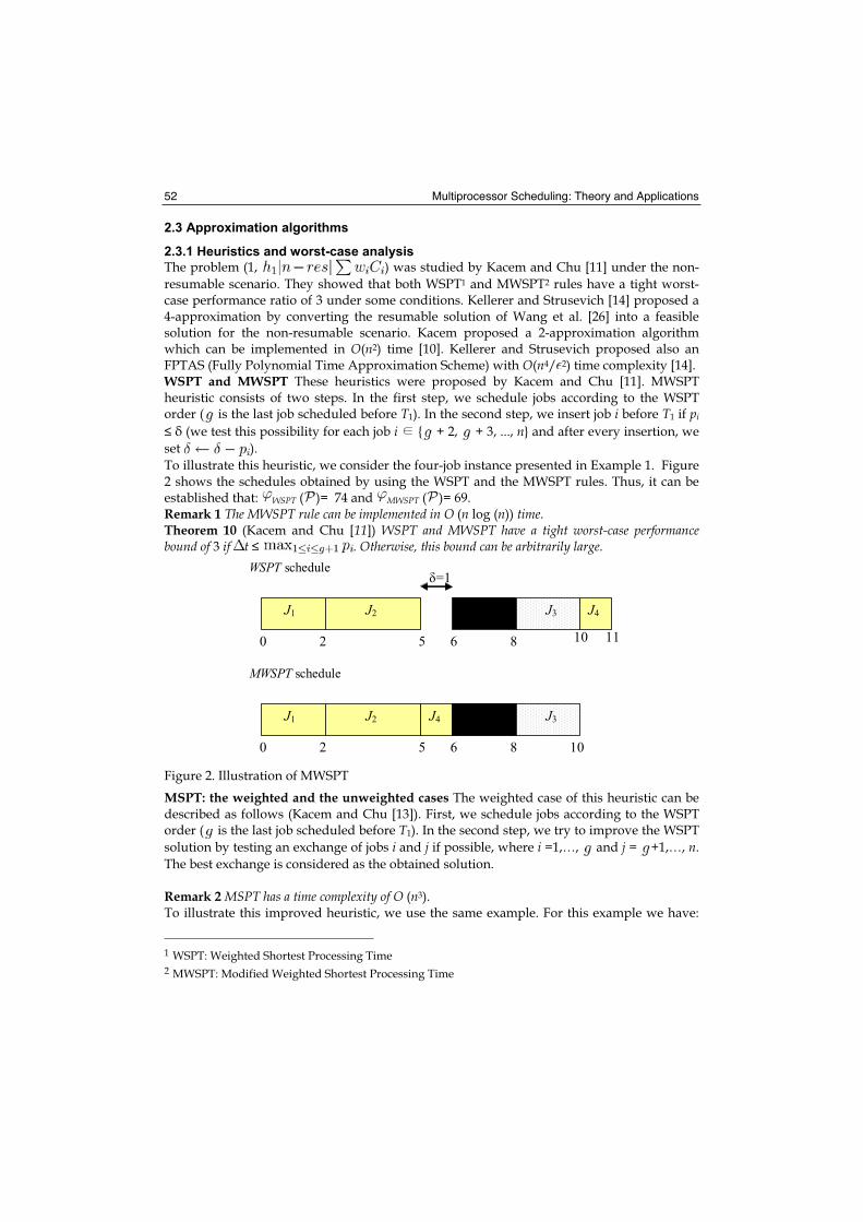
Multiprocessor Scheduling: Theory and Applications 52
2.3 Approximation algorithms
2.3.1 Heuristics and worst-case analysis
The problem (1, ) was studied by Kacem and Chu [11] under the non-
resumable scenario. They showed that both WSPT1 and MWSPT2 rules have a tight worst-case performance ratio of 3 under some conditions. Kellerer and Strusevich [14] proposed a 4-approximation by converting the resumable solution of Wang et al. [26] into a feasible solution for the non-resumable scenario. Kacem proposed a 2-approximation algorithm which can be implemented in O(n2) time [10]. Kellerer and Strusevich proposed also an FPTAS (Fully Polynomial Time Approximation Scheme) with O(n4/ 2) time complexity [14]. WSPT and MWSPT These heuristics were proposed by Kacem and Chu [11]. MWSPT heuristic consists of two steps. In the first step, we schedule jobs according to the WSPT order ( is the last job scheduled before T1). In the second step, we insert job i before T1 if pi
(we test this possibility for each job i { + 2, + 3, ..., n} and after every insertion, we
set ).
To illustrate this heuristic, we consider the four-job instance presented in Example 1. Figure 2 shows the schedules obtained by using the WSPT and the MWSPT rules. Thus, it can be established that: WSPT ( )= 74 and MWSPT ( )= 69. Remark 1 The MWSPT rule can be implemented in O (n log (n)) time.Theorem 10 (Kacem and Chu [11]) WSPT and MWSPT have a tight worst-case performance bound of 3 if t . Otherwise, this bound can be arbitrarily large.
J1
0 2 6 8
WSPT schedule
J2 J3 J4
5 10 11
MWSPT schedule
J1
2 6 8
J2
5 10
J3J4
0
=1
Figure 2. Illustration of MWSPT
MSPT: the weighted and the unweighted cases The weighted case of this heuristic can be described as follows (Kacem and Chu [13]). First, we schedule jobs according to the WSPT order ( is the last job scheduled before T1). In the second step, we try to improve the WSPT
solution by testing an exchange of jobs i and j if possible, where i =1,…, and j = +1,…, n.
The best exchange is considered as the obtained solution.
Remark 2 MSPT has a time complexity of O (n3). To illustrate this improved heuristic, we use the same example. For this example we have:
1 WSPT: Weighted Shortest Processing Time2 MWSPT: Modified Weighted Shortest Processing Time

Scheduling under Unavailability Constraints to Minimize Flow-time Criteria 53
+ 1 = 3. Therefore, four possible exchanges have to be distinguished: (J1 and J3), (J1 and J4),
(J2 and J3) and (J2 and J4). Figure 3 depicts the solutions corresponding to these exchanges. By computing the corresponding weighted flow-time, we obtain MSPT ( )= WSPT ( ).The weighted version of this heuristic has been used by Kacem and Chu in their branch-and-bound algorithm [13]. For the unweighted case (wi = 1), Sadfi et al. studied the worst-case performance of the MSPT heuristic and established the following theorem: Theorem 11 (Sadfi et al. [21]) MSPT has a tight worst-case performance bound of 20/17 when wi=1 for every job i.Recently, Breit improved the result obtained by Sadfi et al. and proposed a better worst-case performance bound for the unweighted case [3].
J1
0 2 6 8
WSPT schedule
J2 J3 J4
5 10 11
Exchange J1 and J3
=1
J1
0 3 6 8
J2 J3 J4
5 10 11
0 3 6 8
J2 J3J4
4 10 12
Exchange J1 and J4
J1
Exchange J2 and J3
J3 J2 J4
0 2 4
J1
0 2 6 8
J3J2J4
3 11 13
Exchange J2 and J4
J1
6 8 11 12
Figure 3. Illustration of MSPT for the weighted case

Multiprocessor Scheduling: Theory and Applications 54
Critical job-based heuristic (HS) [10] This heuristic represents an extension of the one proposed by Wang et al. [26] for the resumable scenario. It is based on the following algorithm (Kacem [10]):
i. Let l = 0 and = .ii. Let (i, l) be the ith job in J – according to the WSPT order. Construct a schedule l =
(1, l) , (2, l), ..., (g (l) , l), , ( (l) + 1, l), ..., (n –| |, l) such that
and where jobs in
are sequenced according to the WSPT order.
iii. If , then: ; go
to step (ii). Otherwise, go to step (iv).
iv. .
Remark 3 HS can be implemented in O (n2) time.We consider the previous example to illustrate HS. Figure 4 shows the sequences h (0 hl) generated by the algorithm. For this instance, we have l = 2 and HS ( ) = WSPT ( ).
J1
0 2 6 8
Schedule 0
J2 J3 J4
5 10 11
Schedule 1
=1
J1
0 2 6 8
J2J3 J4
4 11 12
Schedule 2
J1
0 3 6 8
J2 J3 J4
5 10 11
Figure 4. Illustration of heuristic HS
Theorem 12 (Kacem [10]) Heuristic HS is a 2-approximation algorithm for problem S and its worst-case performance ratio is tight.
2.3.2 Dynamic programming and FPTAS
The problem can be optimally solved by applying the following dynamic programming algorithm AS, which is a weak version of the one proposed by Kacem et al [12]. This algorithm generates iteratively some sets of states. At every iteration k, a set k composed of states is generated (1 k n). Each state [t, f] in k can be associated to a feasible schedule for the first k jobs.

Scheduling under Unavailability Constraints to Minimize Flow-time Criteria 55
Variable t denotes the completion time of the last job scheduled before T1 and f is the total weighted flow-time of the corresponding schedule. This algorithm can be described as follows: Algorithm ASi. Set 1 = {[0, w1(T2 + p1)] , [p1, w1p1]}.
ii. For k {2, 3, ..., n},For every state [t, f] in k –1:
1) Put in k
2) Put in k if t + pk T1
Remove k –1
iii. *( ) = min[t, f] n {f}.Let UB be an upper bound on the optimal weighted flow-time for problem ( ). If we add the restriction that for every state [t, f] the relation f UB must hold, then the running time of AS can be bounded by nT1UB (by keeping only one vector for each state). Indeed, t and fare integers and at each step k, we have to create at most T1UB states to construct k.
Moreover, the complexity of AS is proportional to .
However, this complexity can be reduced to O (nT1) as it was done by Kacem et al [12], by choosing at each iteration k and for every t the state [t, f] with the smallest value of f.In the remainder of this chapter, algorithm AS denotes the weak version of the dynamic programming algorithm by taking UB = HS ( ), where HS is the heuristic proposed by Kacem [10]. The algorithm starts by computing the upper bound yielded by algorithm HS.In the second step of our FPTAS, we modify the execution of algorithm AS in order to reduce the running time. The main idea is to remove a special part of the states generated by the algorithm. Therefore, the modified algorithm AS becomes faster and yields an approximate solution instead of the optimal schedule. The approach of modifying the execution of an exact algorithm to design FPTAS, was initially proposed by Ibarra and Kim for solving the knapsack problem [7]. It is noteworthy that during the last decades numerous scheduling problems have been addressed by applying such an approach (a sample of these papers includes Gens and Levner [6], Kacem [8], Sahni [23], Kovalyov and Kubiak [15], Kellerer and Strusevich [14] and Woeginger [28]-[29]).
Given an arbitrary > 0, we define
and . We split the interval [0, HS ( )] into m1 equal subintervals
of length 1. We also split the interval [0, T1] into m2 equal
subintervals of length 2. The algorithm AS generates
reduced sets instead of sets k. Also, it uses artificially an additional variable w+ for
every state, which denotes the sum of weights of jobs scheduled after T2 for the corresponding state. It can be described as follows: Algorithm ASi. Set ,
ii. For k {2, 3, ..., n},
For every state [t, f,w+] in :

Multiprocessor Scheduling: Theory and Applications 56
1) Put in
2) Put in if t + pk T1
Remove
Let [t, f,w+]r,s be the state in such that f and t with the smallest possible
t (ties are broken by choosing the sate of the smallest f). Set =
.iii. .
The worst-case analysis of this FPTAS is based on the comparison of the execution of algorithms AS and AS . In particular, we focus on the comparison of the states generated by each of the two algorithms. We can remark that the main action of algorithm AS consists in
reducing the cardinal of the state subsets by splitting into m1m2
boxes and by replacing all the vectors of k belonging to by a single
"approximate" state with the smallest t.Theorem 13 (Kacem [9]) Given an arbitrary > 0, algorithm AS can be implemented in O (n2/ 2)
time and it yields an output such that: / * ( ) 1 + .
From Theorem 13, algorithm AS is an FPTAS for the problem 1, .
Remark 4 The approach of Woeginger [28]-[29] can also be applied to obtain FPTAS for this problem. However, this needs an implementation in O (|I|3 n3/ 3), where |I| is the input size.
3. The two-parallel machine case
This problem for the unweighted case was studied by Lee and Liman [19]. They proved that the problem is NP-complete and provided a pseudo-polynomial dynamic programming algorithm to solve it. They also proposed a heuristic that has a worst case performance ratio of 3/2. The problem is to schedule n jobs on two-parallel machines, with the aim of minimizing the total weighted completion time. Every job i has a processing time pi and a weight wi. The first machine is available for a specified period of time [0, T1] (i.e., after T1 it can no longer process any job). Every machine can process at most one job at a time. With no loss of generality, we consider that all data are integers and that jobs are indexed according to the WSPT rule: . Due to the dominance of the WSPT order, an optimal
solution is composed of two sequences (one sequence for each machine) of jobs scheduled in non-decreasing order of their indexes (Smith [25]). In the remainder of the paper, ( )denotes the studied problem, * (Q) denotes the minimal weighted sum of the completion times for problem Q and S (Q) is the weighted sum of the completion times of schedule Sfor problem Q.
3.1 The unweighted case
In this subsection, we consider the unweighted case of the problem, i.e., for every job i, we have wi = 1. Hence, the WSPT order becomes: p1 p2 ... pn.In this case, we can easily remark the following property. Proposition 2 (Kacem [9]) If , then problem ( ) can be optimally solved in O(nlog (n)) time.

Scheduling under Unavailability Constraints to Minimize Flow-time Criteria 57
Based on the result of Proposition 2, we only consider the case where .
3.1.1 Dynamic programming
The problem can be optimally solved by applying the following dynamic programming algorithm A, which is a weak version of the one proposed by Lee and Liman [19]. This algorithm generates iteratively some sets of states. At every iteration k, a set composed of states is generated (1 k n). Each state [t, f] in can be associated to a feasible schedule for the first k jobs. Variable t denotes the completion time of the last job scheduled on the first machine before T1 and f is the total flow-time of the corresponding schedule. This algorithm can be described as follows: Algorithm Ai. Set .
ii. For k {2, 3, ..., n},For every state [t, f] in :
1) Put in
2) Put in if t + pk T1
Removeiii. * ( ) = .
Let UB be an upper bound on the optimal flow-time for problem ( ). If we add the restriction that for every state [t, f] the relation f UB must hold, then the running time of Acan be bounded by nT1UB. Indeed, t and f are integers and at each iteration k, we have to create at most T1UB states to construct . Moreover, the complexity of A is proportional to
.
However, this complexity can be reduced to O (nT1) as it was done by Lee and Liman [19], by choosing at each iteration k and for every t the state [t, f] with the smallest value of f. In the remainder of the paper, algorithm A denotes the weak version of the dynamic programming algorithm by taking UB = H ( ), where H is the heuristic proposed by Lee and Liman [19].
3.1.2 FPTAS (Kacem [9])
The FPTAS is based on two steps. First, we use the heuristic H by Lee and Liman [19]. Then, we apply a modified dynamic programming algorithm. Note that heuristic H has a worst-case performance ratio of 3/2 and it can be implemented in O(n log (n)) time [19]. In the second step of our FPTAS, we modify the execution of algorithm A in order to reduce the running time. Therefore, the modified algorithm becomes faster and yields an approximate solution instead of the optimal schedule.
Given an arbitrary > 0, we define and
. We split the interval [0, H ( )] into q1 equal subintervals
of length 1. We also split the interval [0, T1] into q2 equal subintervals
of length 2.
Our algorithm A generates reduced sets instead of sets . The algorithm can be
described as follows:

Multiprocessor Scheduling: Theory and Applications 58
Algorithm Ai. Set
ii. For k {2, 3, ..., n},
For every state [t, f] in
1) Put in
2) Put in if t + pk T1
Remove
Let [t, f]r,s be the state in such that f and t with the smallest possible t (ties are
broken by choosing the state of the smallest f).
Set = .
iii. .
The worst-case analysis of our FPTAS is based on the comparison of the execution of algorithms A and A . In particular, we focus on the comparison of the states generated by each of the two algorithms. We can remark that the main action of algorithm A consists in
reducing the cardinal of the state subsets by splitting into q1q2 boxes
and by replacing all the vectors of belonging to by a single
"approximate" state with the smallest t.Theorem 14 (Kacem [9]) Given an arbitrary > 0, algorithm A can be implemented in O (n3/ 2)
time and it yields an output such that: .
From Theorem 14, algorithm A is an FPTAS for the unweighted version of the problem.
3.2 The weighted case
In this section, we consider the weighted case of the problem, i.e., for every job i, we have an arbitrary wi. Jobs are indexed in non-decreasing order of pi/wi.In this case, we can easily remark the following property. Proposition 3 (Kacem [9]) If , then problem ( ) has an FPTAS.
Based on the result of Proposition 3, we only consider the case where .
3.2.1 Dynamic programming
The problem can be optimally solved by applying the following dynamic programming algorithm AW, which is a weak extended version of the one proposed by Lee and Liman [19]. This algorithm generates iteratively some sets of states. At every iteration k, a set composed of states is generated (1 k n). Each state [t, p, f] in can be associated to a feasible schedule for the first k jobs. Variable t denotes the completion time of the last job scheduled before T1 on the first machine, p is the completion time of the last job scheduled on the second machine and f is the total weighted flow-time of the corresponding schedule. This algorithm can be described as follows: Algorithm AWi. Set .
ii. For k {2, 3, ..., n},For every state [t, p, f] in :

Scheduling under Unavailability Constraints to Minimize Flow-time Criteria 59
1) Put in
2) Put in if t + pk T1
Remove
iii. .Let UB be an upper bound on the optimal weighted flow-time for problem ( ). If we add the restriction that for every state [t, p, f] the relation f UB must hold, then the running time of AW can be bounded by nPT1UB (where P denotes the sum of processing times). Indeed, t, p and f are integers and at each iteration k, we have to create at most PT1UB states
to construct . Moreover, the complexity of AW is proportional to .
However, this complexity can be reduced to O(nT1) by choosing at each iteration k and for every t the state [t, p, f] with the smallest value of f.In the remainder of the paper, algorithm AW denotes the weak version of this dynamic programming algorithm by taking UB = HW ( ), where HW is the heuristic described later in the next subsection.
3.2.2 FPTAS (Kacem [9])
Our FPTAS is based on two steps. First, we use the heuristic HW. Then, we apply a modified dynamic programming algorithm. The heuristic HW is very simple! We schedule all the jobs on the second machine in the WSPT order. It may appear that this heuristic is bad, however, the following Lemma shows that it has a worst-case performance ratio less than 2. Note also that it can be implemented in O(n log (n)) time. Lemma 1 (Kacem [9]) Let (HW) denote the worst-case performance ratio of heuristic HW. Therefore, the following relation holds: (HW) 2. From Lemma 3, we can deduce that any heuristic for the problem has a worst-case performance bound less than 2 since it is better than HW.In the second step of our FPTAS, we modify the execution of algorithm AW in order to reduce the running time. The main idea is similar to the one used for the unweighted case (i.e., modifying the execution of an exact algorithm to design FPTAS). In particular, we follow the splitting technique by Woeginger [28] to convert AW in an FPTAS. Using a similar notation to [28] and given an arbitrary > 0, we define
and .
First, we remark that every state [t, p, f] verifies
Then, we split the interval [0,T1] into L1+1 subintervals .
We also split the intervals [0, P] and [1, HW ( )] respectively, into L2+1 subintervals
and into L3 subintervals .
Our algorithm AW generates reduced sets instead of sets . This algorithm can be
described as follows: Algorithm AWi. Set
ii. For k {2, 3, ..., n},

Multiprocessor Scheduling: Theory and Applications 60
For every state [t, p, f] in
1) Put in
2) Put in if t + pk T1
Remove
Let [t, p, f]r,s,l be the state in such that t , p and f with the smallest
possible t (ties are broken by choosing the state of the smallest f). Set = .
iii.
3.2.3 Worst-case analysis and complexity
The worst-case analysis of the FPTAS is based on the comparison of the execution of algorithms AW and AW . In particular, we focus on the comparison of the states generated by each of the two algorithms.
Theorem 15 (Kacem [9]) Given an arbitrary > 0, algorithm AW yields an outputsuch that: and it can be implemented in O(|I|3 n3/ 3) time,where |I| is the input size of I.From Theorem 15, algorithm AW an FPTAS for the weighted version of the problem.
4. Conclusion
In this chapter, we considered the non-resumable version of scheduling problems under availability constraint. We addressed the criterion of the weighted sum of the completion times. We presented the main works related to these problems. This presentation shows that some problems can be efficiently solved (as an example, some proposed FPTAS have a strongly polynomial running time). As future works, the idea to extend these results to other variants of problems is very interesting. The development of better approximation algorithms is also a challenging subject.
5. Acknowledgement
This work is supported in part by the Conseil Général Champagne-Ardenne, France (Project OCIDI, grant UB902 / CR20122 / 289E).
6. References
Adiri, I., Bruno, J., Frostig, E., Rinnooy Kan, A.H.G., 1989. Single-machine flow-time scheduling with a single breakdown. Acta Informatica 26, 679-696. [1]
Belouadah, H., Posner, M.E., Potts, C.N., 1992. Scheduling with release dates on a single machine to minimize total weighted completion time. Discrete Applied Mathematics36, 213- 231. [2]
Breit, J., 2006. Improved approximation for non-preemptive single machine flow-time scheduling with an availability constraint. European Journal of Operational Research,doi:10.1016/j.ejor.2006.10.005 [3]
Chen, W.J., 2006. Minimizing total flow time in the single-machine scheduling problem with periodic maintenance. Journal of the Operational Research Society 57, 410-415. [4]

Scheduling under Unavailability Constraints to Minimize Flow-time Criteria 61
Eastman, W. L., Even, S., Issacs, I. M., 1964. Bounds for the optimal scheduling of n jobs on m processors. Management Science 11, 268-279. [5]
Gens, G.V., Levner, E.V., 1981. Fast approximation algorithms for job sequencing with deadlines. Discrete Applied Mathematics 3, 313—318. [6]
Ibarra, O., Kim, C.E., 1975. Fast approximation algorithms for the knapsack and sum of subset problems. Journal of the ACM 22, 463—468. [7]
Kacem, I., 2007. Approximation algorithms for the makespan minimization with positive tails on a single machine with a fixed non-availability interval. Journal of Combinatorial Optimization, doi : 10.1007/s10878-007-9102-4. [8]
Kacem, I., 2007. Fully Polynomial-Time Approximation Schemes for the Flowtime Minimization Under Unavailability Constraint. Workshop Logistique et Transport, 18-20 November 2007, Sousse, Tunisia. [9]
Kacem, I., 2007. Approximation algorithm for the weighted flowtime minimization on a single machine with a fixed non-availability interval. Computers & Industrial Engineering, doi: 10.1016/j.cie.2007.08.005. [10]
Kacem, I., Chu, C., 2006. Worst-case analysis of the WSPT and MWSPT rules for single machine scheduling with one planned setup period. European Journal of Operational Research, doi:10.1016/j.ejor.2006.06.062. [11]
Kacem, I., Chu, C., Souissi, A., 2008. Single-machine scheduling with an availability constraint to minimize the weighted sum of the completion times. Computers & Operations Research, vol 35, n 3, 827 844, doi:10.1016/j.cor.2006.04.010. [12]
Kacem, I., Chu, C., 2007. Efficient branch-and-bound algorithm for minimizing the weighted sum of completion times on a single machine with one availability constraint. International Journal of Production Economics, 10.1016/j.ijpe.2007.01.013. [13]
Kellerer, H., Strusevich, V.A., Fully polynomial approximation schemes for a symmetric quadratic knapsack problem and its scheduling applications. Working Paper,Submitted. [14]
Kovalyov, M.Y., Kubiak, W., 1999. A fully polynomial approximation scheme for weighted earliness-tardiness problem. Operations Research 47: 757-761. [15]
Lee, C.Y., 1996. Machine scheduling with an availability constraints. Journal of Global Optimization 9, 363-384. [16]
Lee, C.Y., 2004. Machine scheduling with an availability constraint. In: Leung JYT (Ed), Handbook of scheduling: Algorithms, Models, and Performance Analysis. USA, FL, Boca Raton, chapter 22. [17]
Lee, C.Y., Liman, S.D., 1992. Single machine flow-time scheduling with scheduled maitenance. Acta Informatica 29, 375-382. [18]
Lee, C.Y., Liman, S.D., 1993. Capacitated two-parallel machines sceduling to minimize sum of job completion times. Discrete Applied Mathematics 41, 211-222. [19]
Qi, X., Chen, T., Tu, F., 1999. Scheduling the maintenance on a single machine. Journal of the Operational Research Society 50, 1071-1078. [20]
Sadfi, C., Penz, B., Rapine, C., Blaÿzewicz, J., Formanowicz, P., 2005. An improved approximation algorithm for the single machine total completion time scheduling problem with availability constraints. European Journal of Operational Research 161, 3-10. [21]

Multiprocessor Scheduling: Theory and Applications 62
Sadfi, C., Aroua, M.-D., Penz, B. 2004. Single machine total completion time scheduling problem with availability constraints. 9th International Workshop on Project Management and Scheduling (PMS’2004), 26-28 April 2004, Nancy, France. [22]
Sahni, S., 1976. Algorithms for scheduling independent tasks. Journal of the ACM 23, 116— 127. [23]
Schmidt, G., 2000. Scheduling with limited machine availability. European Journal of Operational Research 121, 1-15. [24]
Smith, W.E., 1956. Various optimizers for single stage production. Naval Research Logistics Quarterly 3, 59-66. [25]
Wang, G., Sun, H., Chu, C., 2005. Preemptive scheduling with availability constraints to minimize total weighted completion times. Annals of Operations Research 133, 183-192. [26]
Webster, S.,Weighted flow time bounds for scheduling identical processors. European Journal of Operational Research 80, 103-111. [27]
Woeginger, G.J., 2000. When does a dynamic programming formulation guarantee the existence of a fully polynomial time approximation scheme (FPTAS) ?. INFORMS Journal on Computing 12, 57—75. [28]
Woeginger, G.J., 2005. A comment on scheduling two machines with capacity constraints. Discrete Optimization 2, 269—272. [29]

4
Scheduling with Communication Delays
R. Giroudeau and J.C. König LIRMM France
1.1 Introduction
More and more parallel and distributed systems (cluster, grid and global computing) are both becoming available all over the world, and opening new perspectives for developers of a large range of applications including data mining, multimedia, and bio-computing. However, this very large potential of computing power remains largely unexploited this being, mainly due to the lack of adequate and efficient software tools for managing this resource. Scheduling theory is concerned with the optimal allocation of scarce resources to activities over time. Of obvious practical importance, it has been the subject of extensive research since the early 1950's and an impressive amount of literature now exists. The theory dealing with the design of algorithms dedicated to scheduling is much younger, but still has a significant history. An application which will be scheduled on a parallel architecture may be represented by an acyclic graph G = (V, E) (or precedence graph) where V designates the set of tasks, which will be executed on a set of m processors, and where E represents the set of precedence constraints. A processing time is allotted to each task i V.From the very beginning of the study about scheduling problems, models kept up with changing and improving technology. Indeed,
• In the PRAM' s model, in which communication is considered instantaneous, the critical path (the longest path from a source to a sink) gives the length of the schedule. So the aim, in this model, is to find a partial order on the tasks, in order to minimize an objective function.
• In the homogeneous scheduling delay model, each arc (i,j) E represents the potential data transfer between task i and task j provided that i and j are processed on two different processors. So the aim, in this model, is to find a compromise between a sequential execution and a parallel execution.
These two models have been extensively studied over the last few years from both the complexity and the (non)-approximability points of view (see (Graham et al., 1979) and (Chen et al., 1998)). With the increasing importance of parallel computing, the question of how to schedule a set of tasks on a given architecture becomes critical, and has received much attention. More precisely, scheduling problems involving precedence constraints are among the most difficult problems in the area of machine scheduling and they are part of the most studied problems in the domain. In this chapter, we adopt the hierarchical communication model (Bampis et al., 2003) in which we assume that the communication delays are not homogeneous anymore; the processors are connected into clusters and the communications

Multiprocessor Scheduling: Theory and Applications 64
inside a same cluster are much faster than those between processors belonging to different ones.This model incorporates the hierarchical nature of the communications using today's parallel computers, as shown by many PCs or workstations networks (NOWs) (Pfister, 1995; Anderson et al., 1995). The use of networks (clusters) of workstations as a parallel computer (Pfister, 1995; Anderson et al., 1995) has not only renewed the user's interest in the domain of parallelism, but it has also brought forth many new challenging problems related to the exploitation of the potential power of computation offered by such a system. Several approaches meant to try and model these systems were proposed taking into account this technological development:
• One approach concerning the form of programming system, we can quote work (Rosenberg, 1999; Rosenberg, 2000; Blumafe and Park, 1994; Bhatt et al., 1997).
• In abstract model approach, we can quote work (Turek et al., 1992; Ludwig, 1995; Mounié, 2000; Decker and Krandick, 1999; Blayo et al., 1999; Mounié et al., 1999; Dutot and Trystram, 2001) on malleable tasks introduced by (Blayo et al., 1999; Decker and Krandick, 1999). A malleable task is a task which can be computed on several processors and of which the execution time depends on the number of processors used for its execution.
As stated above, the model we adopt here is the hierarchical communication model whichaddresses one of the major problems that arises in the efficient use of such architectures: the task scheduling problem. The proposed model includes one of the basic architectural features of NOWs: the hierarchical communication assumption i.e., a level-based hierarchy of communication delays with successively higher latencies. In a formal context where both a set of clusters of identical processors, and a precedence graph G = (V, E) are given, we consider that if two communicating tasks are executed on the same processor (resp. on different processors of the same cluster) then the corresponding communication delay is negligible (resp. is equal to what we call inter-processor communication delay). On the contrary, if these tasks are executed on different clusters, then the communication delay is more significant and is called inter-cluster communication delay. We are given m multiprocessor machines (or clusters denoted by ) that are used to process n precedence-constrained tasks. Each machine (cluster) comprises several identical
parallel processors (denoted by ). A couple of communication delays is associated to each arc (i, j) between two tasks in the precedence graph. In what follows, cij (resp. ij ) is called inter-cluster (resp. inter-processor) communication, and we consider that cij ij . If tasks i and j are allotted on different machines and , then j must be processed at least cij
time units after the completion of i. Similarly, if i and j are processed on the same machine
but on different processors , and (with k k’) then j can only start ij units of time after the completion of i. However, if i and j are executed on the same processor, then j can start immediately after the end of i. The communication overhead (inter-cluster or inter-processor delay) does not interfere with the availability of processors and any processor may execute any task. Our goal is to find a feasible schedule of tasks minimizing the makespan, i.e., the time needed to process all tasks subject to the precedence graph. Formally, in the hierarchical scheduling delay model a hierarchical couple of values
will be associated with cij - (i, j) E such that:
• if = and if = then ti +pi tj

Scheduling with Communication Delays 65
• else if = and if , with k k' then ti +pi+ ij tj
• ti +pi+cij tj
where ti denotes the starting time of the task i and pi its duration. The objective is to find a schedule, i.e., an allocation of each task to a time interval on one processor, such that communication delays are taken into account and that completion time (makespan) is minimized (the makespan is denoted by Cmax and it corresponds to ). Inwhat follows, we consider the simplest case i V, pi = 1, cij = c 2, ij = c’ 1 with c c'.Note that the hierarchical model that we consider here is a generalization of classical scheduling model with communication delays ((Chen et al., 1998), (Chrétienne and Picouleau, 1995)). Consider, for instance, that for every arc (i, j) of the precedence graph we have cij = ij. In such a case, the hierarchical model is exactly the classical scheduling communication delays model. Note that the values c and l are considered as constant in the following. The chapter is organized as follow: In the next section, some results for UET-UCT model will be presented. In the section 1.3, a lower and upper bound for large communication delays scheduling problem will presented. In the section 1.4, the principal results in hierarchical communication delay model will be presented. In the section 1.5, an influence of an introduction of the duplication on the complexity of scheduling problem is presented. In the section 1.6, some results non-approximability results are given for the total sum of completion time minimization. In the section 1.7, we will conclude on the complexity and approximation scheduling problem in presence of communication delays. In Appendix section, some classical — complete problems are listed which are used in this chapter for the polynomial-time transformations.
1.2 Some results for the UET-UCT model
In the homogeneous scheduling delay model, each arc (i,j) E represents the potential data transfer between task i and task j provided that i and j are processed on two different processors. So the aim, in this model, is to find a compromise between a sequential execution and a parallel execution. These two models have been extensively studied over the last few years from both the complexity and the (non)-approximability points of view (see (Graham et al., 1979) and (Chen et al., 1998)). 1. at any time, a processor executes at most one task; 2. (i, j) E, if = then tj ti + pi, otherwise tj ti+pi + cij.The makespan of schedule is: In the UET-UCT model, we have i, pi = 1 and (i, j) E, c{j = 1.
1.2.1 Unbounded number of processors
In the case of there is no communication delays, the problem becomes polynomial (even if
we consider that i, pi 1). In fact, the Bellman algorithm can be used.
Theorem 1.2.1 The problem of deciding whether an instance of ,pi = 1, cij = problem has a schedule of length 5 is polynomial, see (Veltman, 1993).Proof The proof is based on the notion of total unimodularity matrix, see (Veltman, 1993) and see (Schrijver, 1998).
Theorem 1.2.2 The problem of deciding whether an instance of , pi = 1, cij = problem has a schedule of length 6 is —complete see (Veltman, 1993).

Multiprocessor Scheduling: Theory and Applications 66
Proof The proof is based on the following reduction 3SAT , pi = 1, cij = = 6.
Figure 1.1. The variables-tasks and the clauses-tasks
It is clear that the problem is in .Let be * an instance of 3SAT problem, we construct an instance of the problem , pi
= 1, cij = in the following way:
• For each variable x, six tasks are introduced: x1, x2, x3, x, and x6; the precedence constraints are given by Figure 1.1.
• For each clause c = (xc, yc, zc), where the literals xc, yc and zc are occurrences of negated or unnegated, 3 variables are introduced:
and c: precedence constraints between these tasks are also given by Figure 1.1.
• If the occurrence of variable x in the clause c is unnegated then we add .
• If the occurrence of variable x in the clause c is negated, then we add and.
Clearly, xc represents the occurrence of variable x in the clause c; it precedes the corresponding variable tasks. This is a polynomial-time transformation illustrated by Figure 1.1.It can be proved that, there exists a schedule of length at most six if only if there is a truth assignment {0,1} such that each clause in has at least one true literal.
Corollary 1.2.1 There is no polynomial-time algorithm for the problem , pi = 1, cij
= with performance bound smaller than 7/6 unless , see (Veltman, 1993).Proof The proof of Corollary 1.2.1 is an immediate consequence of the Impossibility Theorem, (see (Chrétienne and Picouleau, 1995), (Garey and Johnson, 1979)).
1.2.2 Approximate solutions with guaranteed performance
Good approximation algorithms seem to be be very difficult to design, since the compromise between parallelism and communication delays is not easy to handle. In this

Scheduling with Communication Delays 67
section, we will present a approximation algorithm with a performance ratio bounded by
4/3 for the problem , pi = 1, cij = . This algorithm is based on a formulation on a integer linear program. A feasible schedule is obtained by a relaxation and rounding procedure. Notice that it exists a trivial 2-approximation algorithm: the tasks without predecessors are executed at t = 0, the tasks admitting predecessors scheduled at t = 0 are executed at t = 2 and so on. Given a precedence graph G = (V, E) a predecessor (resp. successor) of a task i is a task j such that (j, i) (resp. (i, j)) is an arc of G. For every task i V, (i)(resp. (i)) denotes the set of immediate successors (resp. predecessors) of i. We denote the tasks without predecessor (resp. successor) by Z (resp. U). We call source every task belonging to Z.The integer linear program The aim of this section is to model the problem , pi = 1, cij = by an integer linear program (ILP) denoted, in what follows, by .We model the scheduling problem by a set of equations defined on the starting times vector (t1,..., tn):For every arc (i, j) E, we introduce a variable xij {0, 1} which indicates the presence or not of an communication delay, and the following constraints: (i, j) E, ti+pi + xij tj.In every feasible schedule, every task i V — U has at most one successor, w.l.o.g. call them j (i), that can be performed by the same processor as i at time tj = ti+pi. The other successors of i, if any, satisfy: k (i)—{j}, tk ti+pi + l. Consequently, we add the
constraints: .
Similarly, every task i of V — Z has at most one predecessor, w.l.o.g. call them j (i), that can be performed by the same processor as i at times tj satisfying ti — (tj +pj) 1. So, we add
the following constraints: .
If we denote by Cmax the makespan of the schedule, i V, ti+pi < Cmax. Thus, in what follows,the following ILP will be considered:
Let inf denote the linear program corresponding to in which we relax the integrity constraints xij {0, 1} by setting xij [0, 1]. Given that the number of variables and the number of constraints are polynomially bounded, this linear program can be solved in polynomial time. The solution of inf will assign to every arc (i, j) E a value xij = eij with 0
eij 1 and will determine a lower bound of the value of Cmax that we denote by .Lemma 1.2.1 is a lower bound on the value of an optimal solution for , pi = 1, cij= .

Multiprocessor Scheduling: Theory and Applications 68
Proof This is true since any optimal feasible solution of the scheduling problem must satisfy all the constraints of the integer linear program .
Algorithm 1 Rounding Algorithm and construction of the schedule Step 1 [Rounding]
Let be eij the value of an arc (i, j) E given by
Step 1 [Computation of starting time] if i Z then
ti = 0 else
ti = max {tj + 1 + xji} with j (i) and (j, i) Ai,end ifStep 2 [Construction of the schedule]Let be G' = (V; E') where {G' is generated by the 0—arcs.}Allotted each connected component of G' on a different processor. Each task is executed at it starting time. In the following, we call an arc (i,j) E a 0–arc (resp. 1–arc) if xij = 0 (resp. xij = 1). Lemma 1.2.2 Every job i V has at most one successor (resp. predecessors) such that eij < 0.5 (resp. eji < 0.5).Proof We consider a task i V and his successors j1,..., jk such that .We know that , then . Since that
. Then, . Therefore l {2,..., k} we have eij
0.5.We use the same arguments for the predecessors. Lemma 1.2.3 The scheduling algorithm described above provides a feasible schedule.
Proof It is clear that each task i admits at most one incoming (resp. outcoming) 0-arcs. Theorem 1.2.3 The relative performance h of our heuristic is bounded above by (Munier and König, 1997). Proof Let be a path constituted by (k + 1) tasks such that x (resp. (k— x)) arcs values, given by linear programming, between two tasks are less (resp. least) than 1/2. So the length of this path is less than k+l+l/2(k—x) = 3/2k — l/2x + 1. Moreover, by the rounding procedure, the length of this path at most 2k — x + 1. Thus, we obtain
, x. Thus, for a given path, of value p* (resp. p) before (resp. after) the
rounding, admitting x arcs values less than 1/2, we have . A
critical path before the rounding phase is denoted by s*. It is true for the critical path after
the rounding procedure p = s then, .
In fact, the bound is tight (see (Munier and König, 1997)).
1.2.3 Bounded number of processors
In this section, a lower and upper bound will be presented,

Scheduling with Communication Delays 69
Theorem 1.2.4 The problem of deciding whether an instance of , pi = 1, cij =problem has a schedule of length 3 is polynomial, see (Picouleau, 1995). Theorem 1.2.5 The problem of deciding whether an instance of , pi = 1, cij =problem has a schedule of length 4 is -complete, see (Veltman, 1993). Proof The proof is based on the ATP-complete problem Clique.
Figure 1.2. Example of polynomial-time reduction clique , pi = 1, cij =
Let be ' the number of edges of a clique of size k. Let be m' =
, the number of processors of an instance is m = 2(m'+l). It is clear that the problem is in . The proof is based on the polynomial-time reduction clique
, pi = 1, cij = . Let be * a instance of the clique problem. An instance of , pi = 1, cij = problem is constructed in the following way:
• v V the tasks Tv, Kv are introduced,
• e E a task Le is created.
• We add the following precedence constraints: Tv Kv, v V and Tv Le if v is an endpoint of e.
• Four sets of tasks are introduced:
••••
the precedence constraints are added: Uu Xx, Uu Yy, Ww Yy.

Multiprocessor Scheduling: Theory and Applications 70
Figure 1.3. Example of construction in order to illustrate the proof of theorem 1.2.5
It easy to see that the graph G admits a clique of size k if only if it exists a schedule of length 4.
1.2.4 Approximation algorithm
In this section, we will present a simple algorithm which gives a schedule on mmachines from a schedule on unbounded number of processors for the , pi = 1, cij
= . The validity of this algorithm is based on the fact there is at most a matching between the tasks executed at ti and the tasks processed at ti + 1. Theorem 1.2.6 From all polynomial-time algorithm h* with performance guarantee for the problem
, pi = 1, cij = , we may obtain a polynomial-time algorithm with performance guarantee (1 + p) for the problem pi = 1, cij = .Proof
For example, the 4/3-approximation algorithm gives a 7/3-approximation algorithm. Munier et al. (Munier and Hanen, 1996) propose a (7/3 — 4/3m)-approximation algorithm for the same problem.
Algorithm 2 Scheduling on m machines from a schedule on unbounded number of processors
for i = 0 — 1 doLet be Xi the set of tasks executed at ij in using a heuristic h*.The Xi tasks are executed in units of time.
end for
1.3 Large communications delays
Scheduling in presence of large communication delays, is one most difficult problem in scheduling theory, since the starting time of tasks and the communication delay are not be synchronized.If we consider the problem of scheduling a precedence graph with large communication delays and unit execution time (UET-LCT), on a restricted number of processors, Bampis et

Scheduling with Communication Delays 71
al. in (Bampis et al., 1996) proved that the decision problem denoted by , cij = c 2, pi
= ; for Cmax = c + 3 is an -complete problem, and for Cmax = c + 2 (for the special case c = 2), they develop a polynomial-time algorithm. This algorithm can not be extended for c 3. Their proof is based on a reduction from the -complete problem Balanced Bipartite Complete Graph, BBCG (Garey and Johnson, 1979; Saad, 1995). Thus, Bampis et al. (Bampis et al., 1996) proved that the
, cij = c 2, pi = problem does not possess a polynomial-time approximation
algorithm with ratio guarantee better than , unless = .
Figure 1.4. A partial precedence graph for the NT1 -completeness of the scheduling problem , cij = c 3, pi =
Theorem 1.3.1 T/ze problem of deciding whether an instance of , cij = c ; pi = has a schedule of length equal or less than (c+4) is -complete with c 3 (see (Giroudeau et al., 2005)).ProofIt is easy to see that , cij = c ; pi = = c + 4 .The proof is based on a reduction from 1. Given an instance * of 1, we construct an
instance of the problem , cij = c ; pi = = c + 4, in the following way (Figure 1.4 helps understanding of the reduction): n denotes the number of variables of * .
1. For all , we introduce (c + 6) variable-tasks: with j {1, 2, ... , c +
2}. We add the precedence constraints:
with j {1, 2, . . . , c + 1}.
2. For all clauses of length three denoted by Ci = , we introduce 2 x (2 + c)
clause-tasks and , j {1, 2, ... c + 2}, with precedence constraints: and
, j {1, 2, . . . , c + 1}. We add the constraints with and
with .
3. For all clauses of length two denoted by Ci = , we introduce (c + 3) clause-tasks
, j {1, 2, ... , c + 3} with precedence constraints: with j {1, 2, ... , c + 2} and
with .

Multiprocessor Scheduling: Theory and Applications 72
The above construction is illustrated in Figure 1.4. This transformation can be clearly computed in polynomial time.
Remark: is in the clause C' of length two associated with the path
.
It easy to see that there is a schedule of length equal or less than (c + 4) if only if there is a truth assignment such that each clause in has exactly one true literal (i.e. one literal equal to 1), see (Giroudeau et al., 2005). For the special case c = , by using another polynomial-time trnasformation, we state:
Theorem 1.3.2 The problem of deciding whether an instance of , cij = 2; pi = has a schedule of length equal or less than six is -complete (see (Giroudeau et al., 2005)). Corollary 1.3.1 There is no polynomial-time algorithm for the problem , cij 2; pi =with performance bound smaller than unless (see (Giroudeau et al, 2005)). The limit between the -completeness and the polynomial-time algorithm by the following Theorem.
Theorem 1.3.3 The problem of deciding whether an instance of , cij = c; pi = with c {2, 3} has a schedule of length at most (c + 2) is solvable in polynomial time (see (Giroudeau et al., 2005)).
1.3.1 Approximation by expansion In this section, a new polynomial-time approximation algorithm with performance
guarantee non-trivial for the problem , cij 2; pi = will be proposed. Notation: We denote by , the UET-UCT schedule, and by the UET-LCT schedule. Moreover, we denote by ti (resp. ) the starting time of the task i in the schedule (resp. in the schedule ).Principle: We keep an assignment for the tasks given by a "good" feasible schedule on an unrestricted number of processors . We proceed to an expansion of the makespan, while preserving communication delays for two tasks, iand j with (i, j) E, processing on two different processors. Consider a precedence graph G = (V, E), we determine a feasible schedule , for the model UET-UCT, using a (4/3)—approximation algorithm proposed by Munier and König (Munier and König, 1997). This algorithm gives a couple i V, (ti, ) on the schedule corresponding to: ti the starting time of the task i for the schedule and the processor on which the task i is processed at ti. Now, we determine a couple i V, ( , ') on schedule in the following way: The
starting time and, = '. The justification of the expansion coefficient
is given below. An illustration of the expansion is given in Figure 1.5.
Lemma 1.3.1 The coefficient of an expansion is .Proof Consider two tasks i and j such that (i, j) E, which are processed on two different processors in the feasible schedule . Let be d a coefficient d such that and
. After an expansion, in order to respect the precedence constraints and the
communication delays we must have , and so
. It is sufficient to choose .dLemma 1.3.2 An expansion algorithm gives a feasible schedule for the problem denoted by ,cij = c 2; pi = .Proof It is sufficient to check that the solution given by an expansion algorithm produces a feasible schedule for the model UET-LCT. Consider two tasks i and j such that (i,j) E. We

Scheduling with Communication Delays 73
denote by i, (resp. j) the processor on which the task i (resp. the task j) is executed in the
schedule . Moreover, we denote by (resp. ) the processor on which the task i (resp.
the task j) is executed in the schedule . Thus,
• If i = j then = . Since the solution given by Munier and König (Munier and
König, 1997) gives a feasible schedule on the model UET-UCT, then we have ,
• If i j then . We have
Figure 1.5. Illustarion of notion of an expansion
Theorem 1.3.4 An expansion algorithm gives a —approximation algorithm for the problem , cij = c 2; pi = .
Proof We denote by (resp. ) the makespan of the schedule computed by the Munier
and König (resp. the optimal value of a schedule ). In the same way we denote by
(resp. ) the makespan of the schedule computed by our algorithm (resp. the optimal
value of a schedule ).
We know that . Thus, we obtain
.This expansion method can be used for other scheduling problems.
1.4 Complexity and approximation of hierarchical scheduling model
On negative side, Bampis et al. in (Bampis et al., 2002) studied the impact of the hierarchical communications on the complexity of the associated problem. They considered the simplest case, i.e., the problem , and they showed that
this problem did not possess a polynomial-time approximation algorithm with a ratio guarantee better than 5/4 (unless = ).

Multiprocessor Scheduling: Theory and Applications 74
Table 1.1: Previous complexity results for unbounded number of machines for hierarchical communication delay model
Recently, (Giroudeau, 2005) Giroudeau proved that there is no hope to find a -approximation with < 6/5 for the couple of communication delays (cij, ij) = (2,1). If duplication is allowed, Bampis et al. (Bampis et al., 2000a) extended the result of (Chrétienne and Colin, 1991) in the case of hierarchical communications, providing an optimal algorithm
for ;pi = 1; . These complexity results are given in
Table 1.1. On positive side, the authors presented in (Bampis et al., 2000b) a 8/5-approximation
algorithm for the problem ;pi = 1 which is based on an
integer linear programming formulation. They relax the integrity constraints and they produce a feasible schedule by rounding. This result is extended to the problem
;pi = 1 leading to a -approximation algorithm (see
below).The challenge is to determinate a threshold for the approximation algorithm concerning the
two more general problems: l and
l with c' < c. Recently, in (Giroudeau et al., 2005), the authors proved that there is no possibility of finding a p-approximation with p < 1 + l/(c + 4) (unless = ) for the case where all tasks of the precedence graph have unit execution times, where the multiprocessor is composed of an unrestricted number of machines, and where c denotes the communication delay between two tasks i and j both submitted to a precedence constraint and which have to be processed by two different machines (this problem is denoted in the following UET-LCT (Unit Execution Time Large Communication Time) homogeneous scheduling communication delays problem). The problem becomes polynomial whenever the makespan is at most (c + 1). The case of (c + 2) is still partially opened. In the same way as for the hierarchical communication delay model, for the couple of communication delay values (1,0), the authors proved in (Bampis et al., 2002) that there is no possibility of finding a -approximation with < 5/4 (this problem is detailed in following the UET-UCT hierarchical scheduling communication delay problem). Theorem 1.4.1 The problem of deciding whether an instance of
having a schedule of length at most (c + 3) is -complete, see (Giroudeau and König, 2004). Corollary 1.4.1 There is no polynomial-time algorithm for the problem
with c > d performance bound smaller than 1 + unless , see (Giroudeau and König, 2004).
The problem of deciding whether an instance of
having a schedule of length at most (c + 1) is solvable in polynomial
time since l and c are constant.

Scheduling with Communication Delays 75
In the same way as the section 1.2.2, the aim is to model the problem
by an integer linear program (ILP) denoted, in
what follows, by .In this section, we will precise only the difference between the ILP given for the problem
and .In every feasible schedule, every task i V — U has at most two successors, w.l.o.g. call them ji and j2 (i), that can be performed by the same cluster as i at time tj1 = tj2 = ti + pi.The other successors of i, if any, satisfy: k .Consequently, the constraints: are added.
Similarly, every task i of V — Z has at most two predecessors, w.l.o.g. call them j1 and j2
(i), that can be performed by the same cluster as i at times tj1 , tj2 satisfying ti— (tj1 +pj1) <
1 and ti— (tj2 +pj2) < 1. So, the following constraints: are added.
The above constraints are necessary but not sufficient conditions in order to get a feasible schedule for the problem. For instance, a solution minimizing (Cmax for the graph of case (a) in Figure 1.6 will assign to every arc the value 0. However, since every cluster has two processors, and so at most two tasks can be processed on the same cluster simultaneously, the obtained solution is clearly not feasible. Thus, the relaxation of the integer constraints, by considering 0 xij 1, and the resolution of the resulting linear program with objective function the minimization of Cmax, gives just a lower bound of the value of Cmax.In order to improve this lower bound, we consider every sub-graph of G that is isomorphic to the graphs given in Figure 1.6 -cases (a) and (b). It is easy to see that in any feasible schedule of G, at least one of the variables associated to the arcs of each one of these graphs must be set to one. So, the following constraints are added:
• For the case (a): i, j, k, l, m V, such that (j, i), (j, k), (l, k), (l, m) E, xji + xjk + xlk + xlm 1.
• For the case (b): i, j, k, l, m V, such that (i, j), (k, j), (k, l), (m, l) E, xij + xkj + xkl + xml 1.
Thus, in what follows, the following ILP will be considered:
Once again the integer linear program given above does not always imply a feasible solution for the scheduling problem. For instance, if the precedence graph given in Figure 1.7 is considered, the optimal solution of the integer linear program will set all the arcs to 0. Clearly, this is not a feasible solution for our scheduling problem. However, the goal in this step is to get a good lower bound of the makespan and a solution -eventually not feasible- that we will transform to a feasible one.

Multiprocessor Scheduling: Theory and Applications 76
case (a) case (b) Figure 1.6. Special sub-graphs considered in the ILP
Figure 1.7 An optimal solution of the ILP does not always imply a feasible solution
Let inf denote the linear program corresponding to in which we relax the integrability constraints xij {0,1} by setting xij [0,1]. Given that the number of variables and the number of constraints are polynomially bounded, this linear program can be solved in polynomial time. The solution of inf will assign to every arc (i, j) E a value xij = eij with 0 eij 1 and
will determine a lower bound of the value of Cmax that we denote by .Lemma 1.4.1 is a lower bound on the value of an optimal solution for
.Proof See the proof of Theorem 1.2.1. We use the algorithm 1 for the rounding algorithm by changing the value rounded: eij < 0.25 instead eij < 0.5 The solution given by Step 1 is not necessarily a feasible solution (take for instance the precedence graph of Figure 1.7), so we must transform it to a feasible one. Notice that the cases given in Figure 1.6 are eliminated by the linear program. In the next step we need the following definition. Definition 1.4.1 A critical path with terminal vertex i V is the longest path from an arbitrary source of G to task i. The length of a path is defined as the sum of the processing times of the tasks belonging to this path and of the values xij for every arc in the path. 1. Step 2 [Feasible Rounding]: We change the integer solution as follows:
a) If i is a source then we keep unchanged the values of xij obtained in Step 1.b) Let i be a task such that all predecessors are already examined. Let Ai be the subset
of incoming arcs of i belonging to a critical path with terminal vertex the task i.i) If the set Ai, contains a 0-arc, then all the outcoming arcs xij take the value 1. ii) If the set Ai, does not contain any 0-arc (all the critical incoming arcs are valued to
1), then the value of all the outcoming arcs xij remains the same as in Step 1, and all the incoming 0-arcs are transformed to I-arcs.
In Step l b) ii changing the value of an incoming 0-arc to 1 does not increase the length of any critical path having as terminal vertex i, because it exists at least one critical path with terminal vertex i such that an arc (j, i) E is valued by the linear program to at least 0.25 (eji
0.25), and so xji is already equal to 1.

Scheduling with Communication Delays 77
Lemma 1.4.2 Every job i V has at most two successors (resp. predecessors) such that eij < 0.25(resp. eji < 0.25) and The scheduling algorithm described above provides a feasible schedule. Theorem 1.4.2 The relative performance h of our heuristic is bounded above by and the bound is tight, see (Bampis et al, 2003). Proof See the proof of the Theorem 1.2.3.
1.5 Duplication
The duplication of the tasks has been introduced first by Papadimitriou and Yannakakis (Papadimitriou and Yannakakis, 1990) in order to reduce an influence of the communication delays on the schedule. In (Papadimitriou and Yannakakis, 1990), the authors develop a 2-
approximation algorithm for the problem . The
problem (the problem is a subproblem of
) becomes easy. In the following, we will describe the procedure. We may assume w.l.o.g. that all the copies of any task i V start their execution at the same time, call it ti.
1.5.1 Colin-Chrétienne Algorithm see (Chrétienne and Colin, 1991)
The algorithm uses two steps: the first step computes the release times, and the second step use a critical determined from the first step in order to produces a optimal schedule in which all the tasks and their copies are executed at their release times.
a 0b 0c 4d 4e 3f 7g 6h 6i 11
Figure 1.8. P0 problem
The P0 problem given by Figure 1.8 will be illustrated the algorithm. The algorithm which computes the release times is given next:
Algorithm 3 Release date algorithm and Earliest schedule
for i := 1 to n doif PRED(i) = then
bi := 0 else
C := max{bk+pk + cki };
Let be s such that : bs + ps + csi = C;bi := max{bs + ps : max{bk+pk + cki - {s}}}.
end if end forEach connected component Gc = (V; Ec) on different processor; Each copy is executed at his release time.

Multiprocessor Scheduling: Theory and Applications 78
Without lost of generality, all copies of the task i admit the same starting , denoted by ti, as the the task i. A arc (i, j) E is a critical arc if bi+pi +cij > bj. From this definition, it is clear that if (i, j) is a critical arc, then in all as soon as possible schedule, each copy of a task j must be preceded by a copy of a task i on the same processor. In order to construct a earliest schedule, each critical path is allotted on a processor, and each copy is executed at his release date. Theorem 1.5.1 Let be bi the starting time computed by the procedure. For all feasible schedule for a graph G, the release date of a task i cannot be less than bi. All sub-graph is spanning forest. The procedure gives a feasible schedule and the overall complexity is O(n2).
Table 1.2: Complexity results in presence of duplication
Figure 1.9 The critical sub-graph
An earliest schedule of the precedence graph P0 is given by Figure 1.10.
Figure 1.10: An earliest schedule of P0
The study of duplication in presence of unbounded number of processors is theoretical. Indeed, the results on unbounded processors do not improved the results on limited number of processors. So, concerning the hierarchical model, since the number of processors per cluster is limited, the authors in (Bampis et al., 2000a) are investigate only on the theoretical aspect of associated scheduling problem.

Scheduling with Communication Delays 79
Table 1.3. Approximation results in presence of duplication
Table 1.4. Thresold for the total sum of completion time minimization of unbounded number of machines
1.6 Total sum of completion time minimization
In this section, a threshold for total sum of completion time minimization problem is presented for some problems in the homogeneous and hierarchical model. The following table summarize all the results in the homogeneous communication delay model and the hierarchical communication delay model.
Theorem 1.6.1 There is no polynomial-time algorithm for the problem with performance bound smaller than 9/8 unless see (Hoogeveen et al, 1998). Proof We suppose that there is a polynomial-time approximation algorithm denoted by A with performance guarantee bound smaller than 1 + . Let I be the instance of the problem
obtained by a reduction (see Theorem 1.2.2).
Let I' be the instance of the problem by adding x new tasks
from an initial instance I. In the precedence constraints, each group of x (with x > )
new tasks is a successor of the old tasks (old tasks are from the polynomial transformation used for the proof of Theorem 1.2.2). We obtain a complete directed graph from old tasks to new tasks. Let A(I') (resp. A* (I')) be the result given by A (resp. an optimal result) on an instance I'.1. If A(I') < 8 x + 6 n then A*(I') < 8 x + 6 n. So we can decide that there exists a
scheduling of an instance I with Cmax 6. Indeed, we suppose that at most one (denoted by i) task of n old tasks is executed at t = 6. Among the x news tasks, at most one task may be executed on the same processor as i before t = 9. Then A* (I') > 9(x - 1). Thus, x <

Multiprocessor Scheduling: Theory and Applications 80
. A contradiction with x > . Thus, it exists a schedule of length 6 on an old
tasks. 2. . We suppose that A(I') > 8 x + 6 n. So, A*(I') 8x + 6n because an algorithm A is a
polynomial-time approximation algorithm with performance guarantee bound smaller than < 9/8. There is no algorithm to decide whether the tasks from an instance I admit a schedule of length equal or less than 6. Indeed, if there exists such an algorithm, by executing the x tasks at time t = 8, we obtain a schedule with a completion time strictly less than 8x + 6n (there is at least one task which is executed before the time t = 6). This is a contradiction since A*(I') 8x +6n.
This concludes the proof of Theorem 1.6.1.
1.7 Conclusion
Figure 1.11. Principal results in UET-UCT model for the minimization of the length of the schedule
With the Figure 1.11, a question arises: " It exists a -approximation algorithm with INT
for the problems ; and ?"
Moreover, the hierarchical communication delays model is a model more complex as the homogeneous communication delays model. However, this model is not too complex since some analytical results were produced.

Scheduling with Communication Delays 81
1.8 Appendix
In this section, we will give some fundamentals results in theory of complexity and approximation with guaranteed performance. A classical method in order to obtain a lower for none approximation algorithm is given by the following results called "Impossibility theorem" (Chrétienne and Picouleau, 1995) and gap technic see (Aussiello et al., 1999). Theorem 1.8.1 (Impossibility theorem) Consider a combinatorial optimization problem for which all feasible solutions have non-negative integer objective function value (in particular scheduling problem). Let c be a fixed positive integer. Suppose that the problem of deciding if there exists a feasible solution of value at most c is -complete. Then, for any < (c + l)/c, there does not exist a polynomial-time -approximation algorithm A unless = , see ((Chrétienne and Picouleau, 1995), (Aussiello et al, 1999)) Theorem 1.8.2 (The gap technic) Let Q' be an -complete decision problem and let Q be an NPO minimization problem. Let us suppose that there exist two polynomial-time computable functions f :
and d : IN and a constant gap > 0 such that, for any instance x of Q'.
Then no polynomial-time r-approximate algorithm for Q with r < 1 + gap can exist, unless = ,see (Aussiello et al, 1999).
1.8.1 List of -complete problems
In this section, some classical . -complete problems are listed, which are used in this chapter for the polynomial-time transformation.
problemInstances: We consider a logic formula with clauses of size two or three, and each positive literal (resp. negative literal) occurs twice (resp. once). The aim is to find exactly one true literal per clause. Let n be a multiple of 3 and let be a set of clauses of size 2 or 3. There are n clauses of size 2 and n/3 clauses of size 3 so that:
• each clause of size 2 is equal to for some with x y.• each of the n literals x (resp. of the literals ) for x belongs to one of the n clauses of
size 2, thus to only one of them.
• each of the n literals x belongs to one of the n/3 clauses of size 3, thus to only one of them.
• whenever is a clause of size 2 for some , then x and y belong to
different clauses of size 3. We would insist on the fact that each clause of size three yields six clauses of size two. Question:Is there a truth assignment for I: {0,1} such that every clause in has exactly one true literal?Clique problem Instances: Let be G = (V, E) a graph and k a integer. Question: There is a clique (a complete sub-graph) of size k in G ?3 - SAT problemInstances: • Let be = {x1,..., xn} a set of n logical variables.
• Let be = {C1, ... , Cm} a set of clause of length three: .Question: There is I: {0,1} a assignment

Multiprocessor Scheduling: Theory and Applications 82
1.8.2 Ratio of approximation algorithm
This value is defined as the maximum ratio, on all instances /, between maximum objective
value given by algorithm h (denoted by (I)) and the optimal value (denoted by (I)),i.e.
Clearly, we have .
1.8.3 Notations
The notations of this chapter will precised by using the three fields notation scheme , proposed by Graham et al. (Graham et al., 1979):
•• If the number of processors is limited,
• If , then the number of processors is not limited,
• If , then we have unbounded number of clusters constituted by two processors each,
• where:
• If =prec (the precedence graph unspecified *
• If (the communication delay between to tasks admitting a precedence constraint is equal to c)
*
• If (the processing time of all the tasks is equal to one). *
• If =dup (the duplication of task is allowed)
• Si = . (the duplication of task is not allowed)
• is the objective function:
• the minimization of the makespan, denoted by Cmax
• the minimization of the total sum of completion time, denoted by where Cj
= tj+pj
1.9 References
Anderson, T., Culler, D., Patterson, D., and the NOW team (1995). A case for NOW(networks of workstations). IEEE Micro, 15:54–64.
Angel, E., Bampis, E., and Giroudeau, R. (2002). Non-approximability results for the hierarchical communication problem with a bounded number of clusters. In B.Monien, R. F., editor, EuroPar’02 Parallel Processing, LNCS, No. 2400, pages 217–224. Springer-Verlag.
Aussiello, G., Crescenzi, P., Gambosi, G., Kann, V., Marchetti-Spaccamela, A., and Protasi, M. (1999). Complexity and Approximation, chapter 3, pages 100–102. Springer.
Bampis, E., Giannakos, A., and König, J. (1996). On the complexity of scheduling with large communication delays. European Journal of Operation Research, 94:252–260.
Bampis, E., Giroudeau, R., and König, J. (2000a). Using duplication for multiprocessor scheduling problem with hierarchical communications. Parallel Processing Letters,10(1):133–140.

Scheduling with Communication Delays 83
Bampis, E., Giroudeau, R., and König, J. (2002). On the hardness of approximating the precedence constrained multiprocessor scheduling problem with hierarchical communications. RAIRO-RO, 36(1):21–36.
Bampis, E., Giroudeau, R., and König, J. (2003). An approximation algorithm for the precedence constrained scheduling problem with hierarchical communications. Theoretical Computer Science, 290(3):1883–1895.
Bampis, E., Giroudeau, R., and König, J.-C. (2000b). A heuristic for the precedence constrained multiprocessor scheduling problem with hierarchical communications. In Reichel, H. and Tison, S., editors, Proceedings of STACS, LNCS No. 1770, pages 443–454. Springer-Verlag.
Bhatt, S., Chung, F., Leighton, F., and Rosenberg, A. (1997). On optimal strategies for cycle-stealing in networks of workstations. IEEE Trans. Comp., 46:545– 557.
Blayo, E., Debreu, L., Mounié, G., and Trystram, D. (1999). Dynamic loab balancing for ocean circulation model adaptive meshing. In et al., P. A., editor, Proceedings of Europar, LNCS No. 1685, pages 303–312. Springer-Verlag.
Blumafe, R. and Park, D. (1994). Scheduling on networks of workstations. In 3d Inter Symp. of High Performance Distr. Computing, pages 96–105.
Chen, B., Potts, C., and Woeginger, G. (1998). A review of machine scheduling: complexity, algorithms and approximability. Technical Report Woe-29, TU Graz.
Chrétienne, P. and Colin, J. (1991). C.P.M. scheduling with small interprocessor communication delays. Operations Research, 39(3):680–684.
Chrétienne, P. and Picouleau, C. (1995). Scheduling Theory and its Applications.John Wiley & Sons. Scheduling with Communication Delays: A Survey, Chapter 4. Decker, T. and Krandick, W. (1999). Parallel real root isolation using the descartes method.
In HiPC99, volume 1745 of LNCS. Sringer-Verlag. Dutot, P. and Trystram, D. (2001). Scheduling on hierarchical clusters using malleable tasks.
In 13th ACM Symposium of Parallel Algorithms and Architecture, pages 199–208. Garey, M. and Johnson, D. (1979). Computers and Intractability, a Guide to the Theory of NP-
Completeness. Freeman. Giroudeau, R. (2000). L’impact des délais de communications hiérarchiques sur la complexité et
l’approximation des problèmes d’ordonnancement. PhD thesis, Université d’Évry Val d’Essonne.
Giroudeau, R. (2005). Seuil d’approximation pour un problème d’ordonnancement en présence de communications hiérarchiques. Technique et Science Informatique,24(1):95–124.
Giroudeau, R. and König, J. (2004). General non-approximability results in presence of hierarchical communications. In Third International Workshop on Algorithms, Models and Tools for Parallel Computing on Heterogeneous Networks, pages 312–319. IEEE.
Giroudeau, R. and König, J. (accepted). General scheduling non-approximability results in presence of hierarchical communications. European Journal of Operational Research.
Giroudeau, R., König, J., Moulaï, F., and Palaysi, J. (2005). Complexity and approximation for the precedence constrained scheduling problem with large communications delays. In J.C. Cunha, P.M., editor, Proceedings of Europar, LNCS, No. 3648, pages 252–261. Springer-Verlag.

Multiprocessor Scheduling: Theory and Applications 84
Graham, R., Lawler, E., Lenstra, J., and Kan, A. R. (1979). Optimization and approximation in deterministic sequencing and scheduling theory: a survey. Annals of Discrete Mathematics, 5:287–326.
Hoogeveen, H., Schuurman, P., and Woeginger, G. (1998). Non-approximability results for scheduling problems with minsum criteria. In Bixby, R., Boyd, E., and Ríos-Mercado, R., editors, IPCO VI, Lecture Notes in Computer Science, No. 1412, pages 353–366. Springer-Verlag.
Hoogeveen, J., Lenstra, J., and Veltman, B. (1994). Three, four, five, six, or the complexity of scheduling with communication delays. Operations Research Letters, 16(3):129–137.
Ludwig, W. T. (1995). Algorithms for scheduling malleable and nonmalleable parallel tasks. PhD thesis, University of Wisconsin-Madison, Department of Computer Sciences.
Mounié, G. (2000). Efficient scheduling of parallel application : the monotic malleable tasks. PhD thesis, Institut National Polytechnique de Grenoble.
Mounié, G., Rapine, C., and Trystram, D. (1999). Efficient approximation algorithm for scheduling malleable tasks. In 11th ACM Symposium of Parallel Algorithms and Architecture, pages 23–32.
Munier, A. and Hanen, C. (1996). An approximation algorithm for scheduling unitary tasks on m processors with communication delays. Private communication.
Munier, A. and Hanen, C. (1997). Using duplication for scheduling unitary tasks on m processors with communication delays. Theoretical Computer Science, 178:119–127.
Munier, A. and König, J. (1997). A heuristic for a scheduling problem with communication delays. Operations Research, 45(1):145–148.
Papadimitriou, C. and Yannakakis, M. (1990). Towards an architectureindependent analysis of parallel algorithms. SIAM J. Comp., 19(2):322–328.
Pfister, G. (1995). In Search of Clusters. Prentice-Hall. Picouleau, C. (1995). New complexity results on scheduling with small communication
delays. Discrete Applied Mathematics, 60:331–342. Rapine, C. (1999). Algorithmes d’approximation garantie pour l’ordonnancement de tâches,
Application au domaine du calcul parallèle. PhD thesis, Institut National Polytechnique de Grenoble.
Rosenberg, A. (1999). Guidelines for data-parallel cycle-stealing in networks of workstations I: on maximizing expected output. Journal of Parallel Distributing Computing, 59(1):31–53.
Rosenberg, A. (2000). Guidelines for data-parallel cycle-stealing in networks of workstations II: on maximizing guarantee output. Intl. J. Foundations of Comp. Science, 11:183–204.
Saad, R. (1995). Scheduling with communication delays. JCMCC, 18:214–224. Schrijver, A. (1998). Theory of Linear and Integer Programming. John Wiley & Sons. Thurimella, R. and Yesha, Y. (1992). A scheduling principle for precedence graphs with
communication delay. In International Conference on Parallel Processing, volume 3, pages 229–236.
Turek, J., Wolf, J., and Yu, P. (1992). Approximate algorithms for scheduling parallelizable tasks. In 4th ACM Symposium of Parallel Algorithms and Architecture, pages 323–332.
Veltman, B. (1993). Multiprocessor scheduling with communications delays. PhD thesis, CWI-Amsterdam, Holland.

5
Minimizing the Weighted Number of Late Jobs with Batch Setup Times and Delivery Costs on a
Single Machine
George Steiner and Rui Zhang1
DeGroote School of Business, McMaster University Canada
1. Introduction
We study a single machine scheduling problem with batch setup time and batch delivery cost. In this problem, n jobs have to be scheduled on a single machine and delivered to a customer. Each job has a due date, a processing time and a weight. To save delivery cost, several jobs can be delivered together as a batch including the late jobs. The completion (delivery) time of each job in the same batch coincides with the batch completion (delivery) time. A batch setup time has to be added before processing the first job in each batch. The objective is to find a batching schedule which minimizes the sum of the weighted number of late jobs and the delivery cost. Since the problem of minimizing the weighted number of late jobs on a single machine is already -hard [Karp, 1972], the above problem is also -hard. We propose a new dynamic programming algorithm (DP), which runs in pseudopolynomial time. The DP runs in O(n5) time for the special cases of equal processing times or equal weights. By combining the techniques of binary range search and static interval partitioning, we convert the DP into a fully polynomial time approximation scheme (FPTAS) for the general case. The time complexity of this FPTAS is O(n4/ + n4logn).Minimizing the total weighted number of late jobs on a single machine, denoted by
[Graham et. al, 1979], is a classic scheduling problem that has been well studied in the last forty years. Moore [1968] proposed an algorithm for solving the unweighted problem on n jobs in O(nlogn) time. The weighted problem was in the original list of -hard problems of Karp [1972]. Sahni [1976] presented a dynamic program and a fully polynomial time approximation scheme (FPTAS) for the maximization version of the weighted problem in which we want to maximize the total weight of on-time jobs. Gens and Levner [1979] developed an FPTAS solving the minimization version of the weighted problem in O(n3/ ) time. Later on, they developed another FPTAS that improved the time complexity to O(n2logn + n2/ ) [Gens and Levner, 1981]. In the batching version of the problem, denoted by , jobs are processed in batches which require setup time s, and every job's completion time is the completion time of the last job in its batch. Hochbaum and Landy [1994] proposed a dynamic programming algorithm for this problem, which runs in pseudopolynomial time. Brucker and Kovalyov
1 email:[email protected], [email protected]

Multiprocessor Scheduling: Theory and Applications 86
[1996] presented another dynamic programming algorithm for the same problem, which was then converted into an FPTAS with complexity O(n3/ + n3logn).In this paper, we study the batch delivery version of the problem in which each job must be delivered to the customer in batches and incurs a delivery cost. Extending the classical three-field notation [Graham et. al., 1979], this problem can be denoted by bq, where b is the total number of batches and q is the batch delivery cost. The model, without the batch setup times, is similar to the single-customer version of the supplier's supply chain scheduling problem introduced by Hall and Potts [2003] in which the scheduling component of the objective is the minimization of the sum of the weighted number of late jobs (late job penalties). They show that the problem is -hard in the ordinary sense by presenting pseudopolynomial dynamic programming algorithms for both the single-and multi-customer case [Hall and Potts, 2003]. For the case of identical weights, the algorithms become polynomial. However, citing technical difficulties in scheduling late jobs for delivery [Hall and Potts, 2003] and [Hall, 2006], they gave pseudopolynomial solutions for the version of the problem where only early jobs get delivered. The version of the problem in which the late jobs also have to be delivered is more complex, as late jobs may need to be delivered together with some early jobs in order to minimize the batch delivery costs. In Hall and Potts [2005], the simplifying assumption was made that late jobs are delivered in a separate batch at the end of the schedule. Steiner and Zhang [2007] presented a pseudopolynomial dynamic programming solution for the multi-customer version of the problem which included the unrestricted delivery of late jobs. This proved that the problem with late deliveries is also -hard only in the ordinary sense. However, the algorithm had the undesirable property of having the (fixed) number of customers in the exponent of its complexity function. Furthermore, it does not seem to be convertible into an FPTAS. In this paper, we present for bq a different dynamic programming algorithm with improved pseudopolynomial complexity that also schedules the late jobs for delivery. Furthermore, the algorithm runs in polynomial time in the special cases of equal tardiness costs or equal processing times for the jobs. This proves that the polynomial solvability of
can be extended to , albeit by a completely different algorithm. We also show that the new algorithm for the general case can be converted into an FPTAS.The paper is organized as follows. In section 2, we define the bq problem in detail and discuss the structure of optimal schedules. In section 3, we propose our new dynamic programming algorithm for the problem, which runs in pseudopolynomial time. We also show that the algorithm becomes polynomial for the special cases when jobs have equal weights or equal processing times. In the next section, we develop a three-step fully polynomial time approximation scheme, which runs in O(n4/ + n4logn) time. The last section contains our concluding remarks.
2. Problem definition and preliminaries
The problem can be defined in detail as follows. We are given n jobs, J = {1,2,..., n}, with processing time pj, weight wj, delivery due date . Jobs have to be scheduled
nonpreemptively on a single machine and delivered to the customer in batches. Several jobs could be scheduled and delivered together as a batch with a batch delivery cost q and delivery time . For each batch, a batch setup time s has to be added before processing the first job of the batch. Our goal is to find a batching schedule that minimizes the sum of the

Minimizing the Weighted Number of Late Jobs with Batch Setup Times and Delivery Costs on a Single Machine 87
weighted number of late jobs and delivery costs. Without loss of generality, we assume that all data are nonnegative integers. A job is late if it is delivered after its delivery due date, otherwise it is early. The batch completion time is defined as the completion time of the last job in the batch on the machine. Since the delivery of batches can happen simultaneously with the processing of some other jobs on the machine, it is easy to see that a job is late if and only if its batch completion time is greater than its delivery due date minus . This means that each job j has an implied due date on the machine. This implies that we do not need to explicitly schedule the
delivery times and consider the delivery due dates, we can just use the implied due dates, or due dates in short, and job j is late if its batch completion time is greater than dj. (From this point on, we use the term due date always for the dj.) A batch is called an early batch if all jobs are early in this batch, it is called a late batch if every job is late in this batch, and a batch is referred to as mixed batch if it contains both early and late jobs. The batch due date is defined as the smallest due date of any job in the batch. The following simple observations characterize the structure of optimal schedules we will search for. They represent adaptations of known properties for the version of the problem in which there are no delivery costs and/or late jobs do not need to be delivered. Proposition 2.1. There exists an optimal schedule in which all early jobs are ordered in EDD (earliest due date first) order within each batch.Proof. Since all jobs in the same batch have the same batch completion time and batch due date, the sequencing of jobs within a batch is immaterial and can be assumed to be EDD.Proposition 2.2. There exists an optimal schedule in which all late jobs (if any) are scheduled in the last batch (either in a late batch or in a mixed batch that includes early jobs). Proof. Suppose that there is a late job in a batch which is scheduled before the last batch in an optimal schedule. If we move this job into this last batch, it will not increase the cost of the schedule. Proposition 2.3. There exists an optimal schedule in which all early batches are scheduled in EDD order with respect to their batch due date. Proof. Suppose that there are two early batches in an optimal schedule with batch completion times ti < tk and batch due dates di > dk. Since all jobs in both batches are early, we have di > dk tk > ti. Thus if we schedule batch k before batch i, it does not increase the cost of the schedule. Proposition 2.4. There exists an optimal schedule such that if the last batch of the schedule is not a late batch, i.e., there is at least one early job in it, then all jobs whose due dates are greater than or equal to the batch completion time are scheduled in this last batch as early jobs. Proof. Let the batch completion time of the last batch be t. Since the last batch is not a late batch, there must be at least one early job in this last batch whose due date is greater than or equal to t. If there is another job whose due date is greater than or equal to t but it was scheduled in an earlier batch, then we can simply move this job into this last batch without increasing the cost of the schedule. Proposition 2.2 implies that the jobs which are first scheduled as late jobs can always be scheduled in the last batch when completing a partial schedule that contains only early jobs. The dynamic programming algorithm we present below uses this fact by generating all possible schedules on early jobs only and designating and putting aside the late jobs, which get scheduled only at the end in the last batch. It is important to note that when a job is designated to be late in a partial schedule, then its weighted tardiness penalty is added to the cost of the partial schedule.

Multiprocessor Scheduling: Theory and Applications 88
3. The dynamic programming algorithm
The known dynamic programming algorithms for do not have a straightforward extension to bq, because the delivery of late jobs complicates the matter. We know that late jobs can be delivered in the last batch, but setting them up in a separate batch could add the potentially unnecessary delivery cost q for this batch when in certain schedules it may be possible to deliver late jobs together with early jobs and save their delivery cost. Our dynamic programming algorithm gets around this problem by using the concept of designated late jobs, whose batch assignment will be determined only at the end. Without loss of generality, assume that the jobs are in EDD order, i.e., d1 d2 ... dn and let
. If d1 P + s, then it is easy to see that scheduling all jobs in a single batch will
result in no late job, and this will be an optimal schedule. Therefore, we exclude this trivial case by assuming for the remainder of the paper that some jobs are due before P + s. Thestate space used to represent a partial schedule in our dynamic programming algorithm is described by five entries {k, b, t, d, v}: k: the partial schedule is on the job set {1,2,..., k}, and it schedules some of these jobs as early
while only designating the rest as late; b: the number of batches in the partial schedule; t: the batch completion time of the last scheduled batch in the partial schedule; d: the due date of the last batch in the partial schedule; v: the cost (value) of the partial schedule. Before we describe the dynamic programming algorithm in detail, let us consider how we can reduce the state space. Consider any two states (k, b, t1, d,v1) and (k, b, t2, d,v2). Without loss of generality, let t1 t2. If v1 v2, we can eliminate the second state because any later states which could be generated from the second state can not lead to better v value than the value of similar states generated from the first state. This validates the following elimination rule, and a similar argument could be used to justify the second remark. Remark 3.1. For any two states with the same entries {k,b,t,d, }, we can eliminate the state with larger v.Remark 3.2. For any two states with the same entries {k, b, ,d,v}, we can eliminate the state with larger t.The algorithm recursively generates the states for the partial schedules on batches of earlyjobs and at the same time designates some other jobs to be late without actually scheduling these late jobs. The jobs designated late will be added in the last batch at the time when the partial schedule gets completed into a full schedule. The tardiness penalty for every job designated late gets added to the state variable v at the time of designation. We look for an optimal schedule that satisfies the properties described in the propositions of the previous section. By Proposition 2.2, the late jobs should all be in the last batch of a full schedule. It is equivalent to say that any partial schedule {k, b, t, d, v} with 1 b n — 1 can be completed into a full schedule by one of the following two ways: 1. Add all unscheduled jobs {k + 1, k + 2,..., n} and the previously designated late jobs to
the end of the last batch b if the resulting batch completion time (P + bs) does not exceed the batch due date d (we call this a simple completion); or
2. Open a new batch b+1, and add all unscheduled jobs {k + 1, k + 2,..., n} and the previously designated late jobs to the schedule in this batch. (We will call this a direct completion.)

Minimizing the Weighted Number of Late Jobs with Batch Setup Times and Delivery Costs on a Single Machine 89
We have to be careful, however, as putting a previously designated late job into the last batch this way may make such a job actually early if its completion time (P+bs or P + (b + l)s, respectively) is not greater than its due date. This situation would require rescheduling such a designated late job among the early jobs and removing its tardiness penalty from the cost v. Unfortunately, such rescheduling is not possible, since we do not know the identity of the designated late jobs from the state variables (we could only derive their total length and tardy weight). The main insight behind our approach is that there are certain special states, that we will characterize, whose completion never requires such a rescheduling. We proceed with the definition of these special states. It is clear that a full schedule containing exactly l (1 l n) batches will have its last batch completed at P + ls. We consider all these possible completion times and define certain marker jobs mi and batch counters i in the EDD sequence as follows: Let m0 be the last job with
< P + s and m0 +1 the first job with P+s. If m0 +1 does not exist, i.e., m0 = n, then we do not need to define any other marker jobs, all due dates are less than P + s, and we will discuss this case separately later. Otherwise, define 0 = 0 and let 1 1 be the largest integer
for which P + 1s. Let the marker job associated with 1 be the job m1 m0 + 1 whose
due date is the largest due date strictly less than P + ( 1 +1)s, i.e., < P + ( 1 + 1)s and
P + ( 1 + 1)s. Define recursively for i = 2,3,...,h — 1, i i-1 + 1 to be the smallest counter for
which there is a marker job mi mi-1 +1 such that < P + ( i + 1) s and P+( i + 1) s. The last marker job is mh = n and its counter h is the largest integer for which P + h s dn < P + ( h + 1)s. We also define h+1 = h +1. Since the maximum completion time to be considered is P+ns for all possible schedules (when every job forms a separate batch), any due dates which are greater than or equal to P + ns can be reduced to P + ns without affecting the solution. Thus we assume that dn P+ns for the rest of the paper, which also implies h +1 n+1.For convenience, let us also define T1,0 = P + 1s, Ti,k = P + ( i + k)s for i = 1,..., h and k = 0,1,...,
k(i), where each k(i) is the number for which Ti, k (i) = P + ( i + k(i))s = P + i+1 s = Ti+1,0 , and Th,1
= P + ( h + l)s. Note that this partitions the time horizon [P, P + ( h + l)s] into consecutive intervals of length s. We demonstrate these definitions in Figure 1.
Figure 1. Marker Jobs and Corresponding Intervals
We can distinguish the following two cases for these intervals: 1. Ti,1 = Ti+1,0, i.e., k(i) = 1: This means that the interval immediately following Ii = [Ti,0, Ti,1)
contains a due date. This implies that i+1 = i + 1;
2. Ti,1 Ti+1,0, i.e., k(i) > 1: This means that there are k(i) — 1 intervals of length s starting at P + ( i + 1)s in which no job due date is located.
In either case, it follows that every job j > m0 has its due date in one of the intervals Ii = [Ti,0, Ti,1)for some i {1,..., h}, and the intervals [Ti,l, Ti,l+1) contain no due date for i = 1,...,h and l>0.Figure 1 shows that jobs from m0+1 to m1 have their due date in the interval [T1,0, T1,1). Each marker job mi is the last job that has its due date in the interval Ii = [Ti,0, Ti,1) for i = 1,..., h, i.e., we have .

Multiprocessor Scheduling: Theory and Applications 90
Now let us group all jobs into h +1 non-overlapping job sets G0 = {1,..., m0}, G1 = {m0 + 1,..., m1} and Gi = {mi-1 + 1,..., mi} for i = 2,..., h. Then we have and i 1. We also
define the job sets J0 = Go, Ji = G0 G1 ... Gi, for i = 1,2,..., h — 1 and Jh = G0 G1 ... Gh = J.The special states for DP are defined by the fact that their (k, b) state variables belong to the set H defined below: If m0 = n, then let H = {(n, 1), (n, 2), ..., (n, n — 1)};If m0 < n, then let H = H1 H2 H3, where 1. If 1 > 1, then H1 = {(m0, 1), (m0, 2), ..., (m0, 1–1)}, otherwise H1 = ;
2. H2 = , ..., , ..., , ..., ;
3. If 1 < h < n, then H3 = , otherwise H3 = .Note that mh = n and thus the pairs in H3 follow the same pattern as the pairs in the other parts of H. The dynamic program follows the general framework originally presented by Sahni [1976].The Dynamic Programming Algorithm DP[Initialization] Start with jobs in EDD order1. Set (0, 0, 0, 0, 0) S(0), S(k) = , k = 1, 2, ..., n, * = , and define m0, i and mi , i = 1,2,..., h;
2. If m0 + 1 does not exist, i.e., m0 = n, then set H = {(n, 1), (n, 2), ..., (n, n — 1)}; Otherwise set H = H1 H2 H3.
Let I = the set of all possible pairs and =I—H , the complementary set of H.[Generation] Generate set S(k) for k = 1 to n + 1 from S(k-1) as follows:
Set = ;[Operations] Do the following for each state (k — 1,b,t, d, v) in S(k-1)
Case (k - 1, b) H1. If t < P + bs, set * = * (n, b + 1, P + (b + 1)s, d', v + q) /* Generate the direct
completion schedule and add it to the solution set *, where d' is defined as the due date of the first job in batch b+ 1;
2. If t = P + bs, set * = * (n, b, P + bs, d, v) /* We have a partial schedule in which all jobs are early. (This can happen only when k — 1 = n.)
Case (k - 1, b) 1. If t + pk d and k n, set = (k, b, t + pk, d, v) /* Schedule job k as an early job in
the current batch;2. If t + pk + s dk and k n, set = (k, b + 1, t + pk + s, dk, v + q) /* Schedule job k as
an early job in a new batch;3. If k n, set = (k, b, t, d, v + wk) /* Designate job k as a late job by adding its weight
to v and reconsider it at the end in direct completions.Endfor[Elimination] Update set S(k)
1. For any two states (k, b, t, d, v) and (k, b, t, d, v') with v v', eliminate the one with v' from set based on Remark 3.1;
2. For any two states (k, b, t, d, v) and (k, b, t', d, v) with t t', eliminate the one with t' from set based on Remark 3.2;
3. Set S(k) = .Endfor

Minimizing the Weighted Number of Late Jobs with Batch Setup Times and Delivery Costs on a Single Machine 91
[Result] The optimal solution is the state with the smallest v in the set *. Find the optimal schedule by backtracking through all ancestors of this state. We prove the correctness of the algorithm by a series of lemmas, which establish the crucial properties for the special states. Lemma 3.1. Consider a partial schedule (mi, b, t, d, v) on job set Ji, where (mi, b) H. If its completion into a full schedule has b+1 batches, then the final cost of this completion is exactly v + q.Proof. We note that completing a partial schedule on b batches into a full schedule on b + 1batches means a direct completion, i.e., all the unscheduled jobs (the jobs in J — Ji, if any) and all the previously designated late jobs (if any) are put into batch b+1, with completion time P + (b + 1)s.Since all the previously designated late jobs are from Ji for a partial schedule (mi, b, t, d, v), their due dates are not greater than . Therefore, all designated late jobs stay late when scheduled in batch b+1. Next we show that unscheduled jobs j (J — Ji) must be early in batch b+1. We have three cases to consider. Case 1. m0 = n and i = 0:
In this case, H = {(n, 1), (n, 2),..., (n,n — 1)} and J0 = J, i.e. all jobs have been scheduled early or designated late in the state (m0, b, t, d, v). Therefore, there are no unscheduled jobs.
Case 2. m0 < n and b = i :Since 0 = 0 by definition, we must have i 1 in this case. The first unscheduled job j (J— Ji) is job mi + 1 with due date . Thus mi +1 and all other jobs from J — Ji have a due date that is at least P + (b + 1)s, and therefore they will all be early in batch b+1.
Case 3. m0 < n and b > i :This case is just an extension of the case of b = i.If i = 0, then the first unscheduled job for the state (m0, b, t, d, v) is m0 +1. Thus every unscheduled job j has a due date , where the last inequality holds since (m0, b) Hi and therefore, b 1 — 1. If 1 i < h, then we cannot have k(i) = 1: By definition, if k(i) =1, then i + k(i)—1 = i = i
+1—1, which contradicts b > i and (mi,b) H. Therefore, we must have k(i) > 1, and bcould be any value from { i + 1,..., i + k(i) — 1}. This means that P + (b + l)s < P + ( i +k(i))s = P + i+1 s. We know, however, that every unscheduled job has a due date that is at least Ti+1, 0 = P + i+1 s. Thus every job from J — Ji will be early indeed. If i = h, then we have mh = n and Jh = J, and thus all jobs have been scheduled early or designated late in the state (mi, b, t, d, v). Therefore, there are no unscheduled jobs.
In summary, we have proved that all previously designated late jobs (if any) remain late in batch b+1, and all jobs from J — Ji (if any) will be early. This means that v correctly accounts for the lateness cost of the completed schedule, and we need to add to it only the delivery cost q for the additional batch b+1. Thus the cost of the completed schedule is v + q indeed. Lemma 3.2. Consider a partial schedule (mi, b, t, d, v) on job set Ji, where (mi, b) H and b n — 1.Then any completion into a full schedule with more than b + 1 batches has a cost that is at least v + q, i.e., the direct completion has the minimum cost among all such completions of (mi, b,t,d, v).Proof. If mi = n, then the partial schedule is of the form (n, b, t,d,v), (n,b) H, b n — 1. (Thisimplies that either m0 = n with i = 0 or (mi, b) H3 with i = h.) Since there is no unscheduled job left, all the new batches in any completion are for previously designated late jobs. And since all the previously designated late jobs have due dates that are not greater than

Multiprocessor Scheduling: Theory and Applications 92
, these jobs will stay late in the completion. The number of new batches makes no difference to the tardiness penalty cost of late jobs. Therefore, the best strategy is to open only one batch with cost q. Thus the final cost of the direct completion is minimum with cost v + q.Consider now a partial schedule (mi, b, t, d, v), (mi, b) H, b n—1 when mi < n. Since all the previously designated late jobs (if any) are from Ji, their due dates are not greater than
. Furthermore, since all unscheduled jobs are from J — Ji, theirdue dates are not less than . Thus scheduling all of these jobs into batch b + 1 makes them early without increasing the tardiness cost. It is clear that this is the best we can do for completing (mi, b, t, d, v) into a schedule with b + 1 or more batches. Thus the final cost of the direct completion is minimum again with cost v + q. Lemma 3.3. Consider a partial schedule (mi, b, t, d, v} on job set Ji (i 1), where (mi, b) H and b > 1. If it has a completion into a full schedule with exactly b batches and cost v', then there must exist either a partial schedule whose direct completion is of the same cost v' or there exists a partial schedule whose direct completion is of the same cost v'. Proof. To complete the partial schedule (mi,b,t,d,v) into a full schedule on b batches, all designated late jobs and unscheduled jobs have to be added into batch b.Case 1. b > i:
Let us denote the early jobs by Ei Ji in batch b in the partial schedule (mi, b, t, d, v).Adding the designated late jobs and unscheduled jobs to batch b will result in a batch completion time of P+bs. This makes all jobs in Ei late since for j Ei. Thus the cost of the full schedule should be . We cannot do this
calculation, however, since there is no information available in DP about what Ei is. But if we consider the partial schedule =
with one less batch, where is the smallest due date in batch b — 1 in the
partial schedule (mi, b, t, d, v), the final cost of the direct completion of the partial
schedule would be exactly by
Lemma 3.1. We show next that this partial schedule does get generated in the algorithm.
In order to see that DP will generate the partial schedule suppose that during the generation of the partial schedule (mi, b, t, d, v), DP starts batch b byadding a job k as early. This implies that the jobs that DP designates as late on the path of states leading to (mi, b, t, d, v) are in the set Li = {k, k + 1, ..., mi } — Ei. In other words, DP hasin the path of generation for (mi ,b,t,d,v) a partial schedule .Then it will also generate from the partial schedule
by simply designating all jobs in Ei Li as late.
Case 2. b = i 1:Suppose the partial schedule (mi, b, t, d, v) has in batch b the sets of early jobs Ei-1 E,where Ei-1 Ji-1 and E ( Ji — Ji-1). Adding the designated late jobs and unscheduled jobs to batch b will result in a batch completion time of P + bs. This makes all jobs in Ei-1 late since . On the other hand, if L (Ji—Ji-1—E) denotes the previously designated late jobs from Ji — Ji-1 in (mi, b, t, d, v), then these jobs become early since +1 for j L. For similar reasons, all previously designated
late jobs not in L stay late, jobs in E remain early and all other jobs from J — Ji will be early too. In summary, the cost for the full completed schedule derived from (mi,b,t,d,v)should be . Again, we cannot do this calculation, since

Minimizing the Weighted Number of Late Jobs with Batch Setup Times and Delivery Costs on a Single Machine 93
there is no information about Ei-1 and L. However, suppose that Ei-1 , and consider
the partial schedule = with one less batch, where d is the smallest due date in batch b — 1 in
the partial schedule (mi, b, t, d, v). The final cost of the direct completion of the partial schedule would be exactly
by Lemma 3.1. Next, we show that this partial schedule
does get generated during the
execution of DP.To see the existence of the partial schedule =
) note that DP must start batch b on the path of
states leading to (mi, b, t, d, v) by scheduling a job k mi-1 early in iteration k from a state
(We cannot have k > mi-1 since this would contradict Ei-1 . Note also that accounts for the
weight of those jobs from {k, k+l,..., mi-1} that got designated late between iterations k and mi-1
during the generation of the state (mi,b,t,d,v).) In this case, it is clear that DP will also generate from a
partial schedule on Ji-1 in which all jobs in Ei-1 are designated late, in addition to those jobs (if any) from {k, k+1,..., mi-1} that are designated late in (mi, b, t, d, v). Since this schedule will designate all of {k, k+1,..., mi-1} late, the lateness cost of this set of jobs must be added, which results in a state . This is the state
whose existence we claimed. The remaining case is when Ei-1 = . In this case, batch b has no early jobs in the partial schedule (mi,b,t,d,v) from the set Ji-1 and if k again denotes the first early job in batch b, then k
Ji – Ji-1. This clearly implies that (mi,b,t,d,v) must have a parent partial schedule
. Consider the direct completion of this schedule: All designated late jobs must come from Ji-1 and thus they stay late with a completion time of P + bs. Furthermore, all jobs from J – Ji-1 will be early, and therefore, the cost of this direct completion will be .The remaining special cases of b = 1, which are not covered by the preceding lemma, are (mi,b) = (m1, 1) or (mi, b) = (m0, 1), and they are easy: Since all jobs are delivered at the same time P + s, all jobs in J0 or J, respectively, are late, and the rest of the jobs are early. Thus there is
only one possible full schedule with cost .In summary, consider any partial schedule (mi, b, t, d, v) on job set Ji, where (mi, b) H , or a partial schedule (n, b, t, d, v) on job set J and assume that the full schedule S' = (n, b' , P + b's, d' , v') is a completion of this partial schedule and has minimum cost v'. Then the following schedules generated by DP will contain a schedule among them with the same minimum cost as S':
1. the direct completion of (mi,b,t,d,v), if (mi, b) (mi, i) and b' > b, by Lemma 3.1 and Lemma 3.2;
2. the direct completion of a partial schedule , if (mi, b) (mi, i) and b' = b, by Lemma 3.3;
3. the direct completion of a partial schedule , if (mi, b) = (mi, i), i > 1 and b' = b, by Lemma 3.3;
4. the full schedule if m0 < n and b' b = 1 = 1 i.e., (mi, b)
= (m1, 1);

Multiprocessor Scheduling: Theory and Applications 94
5. the full schedule , if m0 = n and b' b = 1. i.e., (mi, b) =
(m0, 1).Theorem 3.1. The dynamic programming algorithm DP is a pseudopolynomial algorithm, which finds an optimal solution for in min time and space, where .
Proof. The correctness of the algorithm follows from the preceding lemmas and discussion. It is clear that the time and space complexity of the procedures [Initialization] and [Result] is dominated by the [Generation] procedure. At the beginning of iteration k, the total number of possible values for the state variables {k, b, t, d, v} in S(k) is upperbounded as follows: n is the upper bound of k and b; n is the upper bound for the number of different d values; min{dn, P+ ns} is an upper bound of t and W + nq is an upper bound of v, and because of the elimination rules, min{dn, P+ns, W+nq} is an upper bound for the number of different combinations of t and v. Thus the total number of different states at the beginning of each iteration k in the [Generation] procedure is at most O(n2 min{dn, P + ns, W + nq}). In each iteration k, there are at most three new states generated from each state in S(k-1) and this takes constant time. Since there are n iterations, the [Generations] procedure could indeed be done in O(n3 min{dn, P + ns, W + nq}) time and space. Corollary 3.1. For the case of equal weights, the dynamic programming algorithm DP finds an optimum solution in O(n5) time and space.Proof. For any state, v is the sum of two different cost components: the delivery costs from {q, 2q,..., nq} and the weighted number of late jobs from {0, w,..., nw}, where wj = w, .Therefore, v can take at most n(n + 1) different values and the upper bound for the number of different states becomes O(n3 min{dn, P + ns, n2}) = O(n5).Corollary 3.2. For the case of equal processing times, the dynamic programming algorithm DP finds an optimum solution in O(n5) time and space.Proof. For any state, t is the sum of two different time components: the setup times from {s, ...,ns} and the processing times from {0,p, ...,np}, where pj = p, . Thus, t can take at most n(n + 1) different values, and the upper bound for the number of different states becomes O(n3 min{dn, n2, W + nq}) = O(n5).
4. The Fully Polynomial Time Approximation Scheme
To develop a fully polynomial time approximation scheme (FPTAS), we will use static interval partitioning originally suggested by Sahni [1976] for maximization problems. The efficient implementation of this approach for minimization problems is more difficult, as it requires prior knowledge of a lower (LB) and upper bound (UB) for the unknown optimum value v*, such that the UB is a constant multiple of LB. In order to develop such bounds, we propose first a range algorithm R(u, ), which for given u and , either returns a full schedule with cost v u or verifies that (1 — ) u is a lower bound for the cost of any solution. In the second step, we use repeatedly the range algorithm in a binary search to narrow the range [LB, UB] so that UB 2LB at the end. Finally, we use static interval partitioning of the narrowed range in the algorithm DP to get the FPTAS. Similar techniques were used by Gens and Levner [1981] for the one-machine weighted-number-of-late-jobs problem
and Brucker and Kovalyov [1996] for the one-machine weighted-number-of-late-jobs batching problem without delivery costs .The range algorithm is very similar to the algorithm DP with a certain variation of the [Elimination] and [Result] procedures.

Minimizing the Weighted Number of Late Jobs with Batch Setup Times and Delivery Costs on a Single Machine 95
The Range Algorithm R(u, )[Initialization] The same as that in the algorithm DP.[Partition] Partition the interval [0, u] into equal intervals of size u /n, with the last one possibly smaller. [Generation] Generate set S(k) for k = 1 to k = n + 1 from S(k-1) as follows:
Set = ;[Operations] The same as those in the algorithm DP. [Elimination] Update set S(k)
1. Eliminate any state (k, b, t, d, v) if v > u.2. If more than one state has a v value that falls into the same interval, then discard all
but one of these states, keeping only the representative state with the smallest tcoordinate for each interval.
3. For any two states (k, b, t, d, v) and (k, b, t, d, v') with v < v', eliminate the one with v' from set based on Remark 3.2;
4. Set S(k) = .Endfor[Result]If * = , then v* > (1 - ) u; If * , then v* u.Theorem 4.1. If at the end of the range algorithm R(u, ), we found * = , then v* > (1— )u; otherwise v* u. The algorithm runs in O(n4/ ) time and space. Proof. If * is not empty, then there is at least one state (n, b, t, d, v) that has not been eliminated. Therefore, v is in some subinterval of [0, u] and v* v u. If * = , then all states with the first two entries (k, b) H have been eliminated. Consider any feasible schedule (n,b,t,d,v). The fact that * = means that any ancestor state of (n,b,t,d,v) with cost
must have been eliminated at some iteration k in the algorithm either because > u or by interval partitioning, which kept some other representative state with cost ' and maximum error u/n. In the first case, we also have v > u. In the second case, let v' ' be the cost of a completion of the representative state and we must have v' > u since * = . Since the error introduced in one iteration is at most u/n, the overall error is at most n( u/n) = u, i.e., v v'— n( u/n) = v' — u > u — u = (1 — )u. Thus v > (1 — )u for any feasible cost value v.For the complexity, we note that for k = 1,2,...,n. Since all operations on a single state can be performed in O(1) time, the overall time and space complexity is O(n4/ ).The repeated application of the algorithm R(u, ) will allow us to narrow an initially wide range of upper and lower bounds to a range where our upper bound is only twice as large as the lower bound. We will start from an initial range v' v* nv'. Next, we discuss how we can find such an initial lower bound v'.Using the same data, we construct an auxiliary batch scheduling problem in which we want to minimize the maximum weight of late jobs, batches have the same batch-setup time s, the completion time of each job is the completion time of its batch, but there are no delivery costs. We denote this problem by . It is clear that the minimum cost of this problem will be a lower bound for the optimal cost of our original problem. To solve the problem, we first sort all jobs into smallest-weight-first order, i.e., w[1] w[2] ... w[n]. Here we are using [k] to denote the job with the kth smallest weight. Suppose that [k*] has the largest weight among the late jobs in an optimal schedule. It is

Multiprocessor Scheduling: Theory and Applications 96
clear that there is also an optimal schedule in which every job [i], for i = 1,2,..., k*, is late, since we can always reschedule these jobs at the end of the optimal schedule without making its cost worse. It is also easy to see that we can assume without loss of generality that the early jobs are scheduled in EDD order in an optimal schedule. Thus we can restrict our search for an optimal schedule of the following form: There is a k {0,1,..., n} such that jobs {[k + 1],..., [n]} are early and they are scheduled in EDD order in the first part of the schedule, followed by jobs {[1], [2],..., [k]} in the last batch in any order. The existence of such a schedule can be checked by the following simple algorithm. The Feasibility Checking Algorithm FC(k)[Initialization] For the given k value, sort the jobs {[k + 1],..., [n]} into EDD order, and let this
sequence be , where f = n — k.Set i = 1, j = , t = s + pj and d = dj
lf t > d, no feasible schedule exists and goto [Report];If t d, set i = 2 and goto [FeasibilityChecking].
[FeasibilityChecking] While i f do
Set j = ,If t + pj > d, start a new batch for job j;
if t + s + pj > dj, no feasible schedule exists and goto [Report};if t+s+pj dj, set t = t+s+pj, d = dj, i = i+1 and goto [FeasibilityChecking].
If t + pj d, set t = t + pj, i = i + 1 and goto [FeasibilityChecking].Endwhile
[Report] If i f, no feasible schedule exists. Otherwise, there exists a feasible batching schedule for jobs in which these jobs are early.
The problem can be solved by repeatedly calling FC(k) for increasing k to find the first k value, denoted by k*, for which FC(k) returns that a feasible schedule exists. The Min-Max Weight Algorithm MW[Initialization] Sort the jobs into a nondecreasing sequence by their weight
w[1] w[2] ... w[n] and set k = 0.[AlgorithmFC] While k n call algorithm FC(k).
If FC(k) reports that no feasible schedule exists, set k = k+1 and goto [AlgorithmFC] ;Otherwise, set k* = k and goto [Result];Endwhile
[Result] If k* = 0 then there is a schedule in which all jobs are early and set w* = 0; otherwise, is the optimum.
Theorem 4.2. The Min-Max Weight Algorithm MW finds the optimal solution to the problem in O(n2) time.
Proof. For k = 0, FC(k) constructs the EDD sequence on the whole job set J, which requires O(nlogn) time. We can obtain the sequence (f = n — k) in the initialization step of FC(k + 1), from the sequence constructed for FC(k) in O(n) time by simply deleting the job [k] from it. It is clear that all other operations in FC(k) need at most O(n) time. Since MW calls FC(k) at most (n + 1) times, the overall complexity of the algorithm is O(n2) indeed. Corollary 4.1. The optimal solution v* to the problem of minimizing the sum of the weighted number of late jobs and the batch delivery cost on a single machine, , is in the interval [v', nv'], where v' = w* + q. Proof. It is easy to see that there is at least one batch and there are at most n — k* + 1 batches in a feasible schedule. Also the weighted number of late jobs is at least w* and at most k*w*

Minimizing the Weighted Number of Late Jobs with Batch Setup Times and Delivery Costs on a Single Machine 97
in an optimal schedule for . Thus v' = w* + q is a lower bound and k*w* +(n — k* + 1)q nw* + nq = n(w* + q) = nv' is an upper bound for the optimal solution v* of
.Next, we show how to narrow the range of these bounds. Similarly to Gens and Levner [1981], we use the algorithm R(u, ) with = 1/4 in a binary search to narrow the range [v', nv'].The Range and Bound Algorithm RB[Initialization] Set u' = nv'/2;[BinarySearch] Call R(u', 1/4);
If R(u', 1/4) reports that v* u', set u' = u' /2 and goto [BinarySearch];If R(u', 1/4) reports v* > 3 u'/4, set u' = 3u'/2.
[Determination] Call R(u', 1/4). If R(u', 1/4) reports v* u', set = u'/2 and stop; If R(u', 1/4) reports v* > 3 u'/4, set = 3u'/2 and stop.
Theorem 4.3. The algorithm RB determines a lower bound for v* such that v* 2 and it requires O(n4logn) time. Proof. It can be easily checked that when the algorithm stops, we have v* 2 . For each iteration of the range algorithm R(u', 1/4), the whole value interval is divided into subintervals with equal length (the last subinterval may be less), where u' v'. Since only
values v u' are considered in this range algorithm, the maximum number of subintervals is less than or equal to . By the proof of Theorem 4.1, the time complexity of
one call to R(u', 1/4) is O(n4). It is clear that the binary search in RB will stop after at most O(logn) calls of R(u', 1/4), thus the total running time is bounded by O(n4logn).Finally, to get an FPTAS, we need to run a slightly modified version of the algorithm DPwith static interval partitioning. We describe this below. Approximation Algorithm ADP[Initialization] The same as that in the algorithm DP.[Partition] Partition the interval [ , 2 ] into equal intervals of size /n, with the last
one possibly smaller. [Generation] Generate set S(k) for k = 1 to k = n + 1 from S(k-1) as follows:
Set = ;[Operations] The same as those in the algorithm DP.[Elimination] Update set S(k).1. If more than one state has a v value that falls into the same sub-interval, then
discard all but one of these states, keeping only the representative state with the smallest t coordinate.
2. For any two states (k, b, t, d, v) and (k, b, t, d, v') with v v', eliminate the one with v'from set based on Remark 3.2;
3. Set S(k) = .Endfor[Result] The best approximating solution corresponds to the state with the smallest v over all states in *. Find the final schedule by backtracking through the ancestors of this state. Theorem 4.4. For any > 0, the algorithm ADP finds in O(n4/ ) time a schedule with cost v for the
problem, such that v (1 + )v*.Proof. For each iteration in the algorithm ADP, the whole value interval [ , 2 ] is divided into subintervals with equal length (the last subinterval may be less). Thus the maximum

Multiprocessor Scheduling: Theory and Applications 98
number of the subintervals is less than or equal to . By the proof of Theorem 3.1,
the time complexity of the algorithm is O(n4/ ) indeed. To summarize, the FPTAS applies the following algorithms to obtain an -approximation for the problem.
The Fully Polynomial Time Approximation Scheme (FPTAS)1. Run the algorithm MW by repeatedly calling FC(k) to determine v' = w* + q;2. Run the algorithm RB by repeatedly calling R(u', 1/4) to determine ;3. Run the algorithm ADP using the bounds v* 2 .Corollary 4.2. The time and space complexity of the FPTAS is O(n4logn + n4/ ).Proof. The time and space complexity follows from the proven complexity of the component algorithms.
5. Conclusions and further research
We presented a pseudopolynomial time dynamic programming algorithm for minimizing the sum of the weighted number of late jobs and the batch delivery cost on a single machine. For the special cases of equal weights or equal processing times, the algorithm DP requires polynomial time. We also developed an efficient, fully polynomial time approximation scheme for the problem. One open question for further research is whether the algorithm DP and the FPTAS can be extended to the case of multiple customers.
6. References
P. Brucker and M.Y. Kovalyov. Single machine batch scheduling to minimize the weighted number of late jobs. Mathematical Methods of Operation Research, 43:1-8, 1996.
G.V. Gens and E.V. Levner. Discrete optimization problems and efficient approximate algorithms. Engineering Cybernetics, 17(6):1-11, 1979.
G.V. Gens and E.V. Levner. Fast approximation algorithm for job sequencing with deadlines. Discrete Applied Mathematics, 3(4):313-318, 1981.
R.L. Graham, E.L. Lawler, J.K. Lenstra and A.H.G. Rinnooy Kan. Optimization and approximation in deterministic sequencing and scheduling: a survey. Ann. Discrete Math., 4:287-326, 1979.
N.G. Hall and C.N. Potts. The coordination of scheduling and batch deliveries. Annals Of Operations Research, 135(1):41-64, 2005.
N.G. Hall. Private communication. 2006. N.G. Hall and C.N. Potts. Supply chain scheduling: Batching and delivery. Operations
Research, 51(4):566-584, 2003. D.S. Hochbaum and D. Landy. Scheduling with batching: minimizing the weighted number
of tardy jobs. Operations Research Letters, 16:79-86, 1994. R.M. Karp. Reducibility among combinatorial problem. In R.E. Miller and Thatcher J.W., editors,
Complexity of Computer Computations, pages 85-103. Plenum Press, New York, 1972. J.M. Moore. An n job, one machine sequencing algorithm for minimizing the number of late
jobs. Management Science, 15:102-109, 1968. S.K. Sahni. Algorithms for scheduling independent tasks. Journal of the ACM, 23(1): 116-127, 1976. G. Steiner and R. Zhang. Minimizing the total weighted number of late jobs with late
deliveries in two-level supply chains. 3rd Multidisciplinary International Scheduling Conference: Theory and Applications (MISTA), 2007.

6
On-line Scheduling on Identical Machines for Jobs with Arbitrary Release Times
Rongheng Li1 and Huei-Chuen Huang2
1Department of Mathematics, Hunan Normal University, 2Department of Industrial and Systems Engineering, National University of Singapore
1China., 2Singapore
1. Introduction
In the theory of scheduling, a problem type is categorized by its machine environment, job characteristic and objective function. According to the way information on job characteristic being released to the scheduler, scheduling models can be classified in two categories. One is termed off-line in which the scheduler has full information of the problem instance, such as the total number of jobs to be scheduled, their release times and processing times, before scheduling decisions need to be made. The other is called on-line in which the scheduler acquires information about jobs piece by piece and has to make a decision upon a request without information of all the possible future jobs. For the later, it can be further classified into two paradigms. 1. Scheduling jobs over the job list (or one by one). The jobs are given one by one
according to a list. The scheduler gets to know a new job only after all earlier jobs have been scheduled.
2. Scheduling jobs over the machines' processing time. All jobs are given at their release times. The jobs are scheduled with the passage of time. At any point of the machines' processing time, the scheduler can decide whether any of the arrived jobs is to be assigned, but the scheduler has information only on the jobs that have arrived and has no clue on whether any more jobs will arrive.
Most of the scheduling problems aim to minimize some sort of objectives. A common objective is to minimize the overall completion time Cmax, called makespan. In this chapter we also adopt the same objective and our problem paradigm is to schedule jobs on-line over a job list. We assume that there are a number of identical machines available and measure the performance of an algorithm by the worst case performance ratio. An on-line algorithm
is said to have a worst case performance ratio σ if the objective of a schedule produced by
the algorithm is at most σ times larger than the objective of an optimal off-line algorithm for any input instance. For scheduling on-line over a job list, Graham (1969) gave an algorithm called List Scheduling (LS) which assigns the current job to the least loaded machine and showed that
LS has a worst case performance ratio of where m denotes the number of machines
available. Since then no better algorithm than LS had been proposed until Galambos & Woeginger (1993) and Chen et al. (1994) provided algorithms with better performance for

Multiprocessor Scheduling: Theory and Applications 100
m 4. Essentially their approach is to schedule the current job to one of the two least loaded machines while maintaining some machines lightly loaded in anticipation of the possible arrival of a long job. However for large m, their performance ratios still approach 2 because the algorithms leave at most one machine lightly loaded. The first successful approach to bring down the ratio from 2 was given by Bartal et al. (1995), which keeps a constant fraction of machines lightly loaded. Since then a few other algorithms which are better than LS have been proposed (Karger et al. 1996, Albers 1999). As far as we know, the current best performance ratio is 1.9201 which was given by Fleischer & Wahl (2000). For scheduling on-line over the machines' processing time, Shmoys et al. (1995) designed a non-clairvoyant scheduling algorithm in which it is assumed any job's processing time is not known until it is completed. They proved that the algorithm has a performance ratio of 2. Some other work on the non-clairvoyant algorithm was done by Motwani et al. (1994). On the other hand, Chen & Vestjens (1997) considered the model in which jobs arrive over time and the processing time is known when a job arrives. They showed that a dynamic LPT algorithm, which schedules an available job with the largest processing time once a machine becomes available, has a performance ratio of 3/2. In the literature, when job's release time is considered, it is normally assumed that a job arrives before the scheduler needs to make an assignment on the job. In other words, the release time list synchronizes with the job list. However in a number of business operations, a reservation is often required for a machine and a time slot before a job is released. Hence the scheduler needs to respond to the request whenever a reservation order is placed. In this case, the scheduler is informed of the job's arrival and processing time and the job's request is made in form of order before its actual release or arrival time. Such a problem was first proposed by Li & Huang (2004), where it is assumed that the orders appear on-line and upon request of an order the scheduler must irrevocably pre-assign a machine and a time slot for the job and the scheduler has no clue or whatsoever of other possible future orders. This problem is referred to as an on-line job scheduling with arbitrary release times, which is the subject of study in the chapter. The problem can be formally defined as follows. For a business operation, customers place job orders one by one and specify the release time rj
and the processing time pj of the requested job Jj. Upon request of a customer's job order, the operation scheduler has to respond immediately to assign a machine out of the m available identical machines and a time slot on the chosen machine to process the job without interruption. This problem can be viewed as a generalization of the Graham's classical on-line scheduling problem as the later assumes that all jobs' release times are zero. In the classical on-line algorithm, it is assumed that the scheduler has no information on the future jobs. Under this situation, it is well known that no algorithm has a better performance ratio than LS for m 3 (Faigle et al. 1989) . It is then interesting to investigate whether the performance can be improved with additional information. To respond to this question, the semi-online scheduling is proposed. In the semi-online version, the conditions to be considered online are partially relaxed or additional information about jobs is known in advance and one wishes to make improvement of the performance of the optimal algorithm with respect to the classical online version. Different ways of relaxing the conditions give rise to different semi-online versions (Kellerer et al. 1997). Similarly several types of additional information are proposed to get algorithms with better performance. Examples include the total length of all jobs is known in advance (Seiden et al. 2000), the largest length of jobs is known in advance (Keller 1991, He et al. 2007), the lengths of all jobs are known in

On-line Scheduling on Identical Machines for Jobs with Arbitrary Release Times 101
[p, rp] where p > 0 and r 1 which is called on-line scheduling for jobs with similar lengths (He & Zhang 1999, Kellerer 1991), and jobs arrive in the non- increasing order of their lengths (Liu et al. 1996, He & Tan 2001, 2002, Seiden et al. 2000). More recent publications on the semi-online scheduling can be found in Dosa et al. (2004) and Tan & He (2001, 2002). In the last section of this chapter we also extend our problem to be semi-online where jobs are assumed to have similar lengths. The rest of the chapter is organized as follows. Section 2 defines a few basic terms and the LS algorithm for our problem. Section 3 gives the worst case performance ratio of the LS algorithm. Section 4 presents two better algorithms, MLS and NMLS, for m 2. Section 5 proves that NMLS has a worst case performance ratio not more than 2.78436. Section 6 extends the problem to be semi-online by assuming that jobs have similar lengths. For simplicity of presentation, the job lengths are assumed to be in [l, r] or p is assumed to be 1. In this section the LS algorithm is studied. For m 2, it gives an upper bound for the performance ratio and shows that 2 is an upper bound when . For m = 1, it shows
that the worst case performance ratio is and in addition it gives a lower bound for
the performance ratio of any algorithm.
2. Definitions and algorithm LS
Definition 1. Let L = {J1, J2,... , Jn} be any list of jobs, where job Jj(j = 1, 2, ... , n) arrives at its release time rj and has a processing time of pj. There are m identical machines available. Algorithm A is a heuristic algorithm. and denote the makespans of
algorithm A and an optimal off-line algorithm respectively. The worst case performance ratio of Algorithm A is defined as
Definition 2. Suppose that Jj is the current job with release time rj and processing time pj.Machine Mi is said to have an idle time interval for job Jj, if there exists a time interval [T1,T2]satisfying the following conditions:
1. Machine Mi is idle in interval [T1,T2J and a job has been assigned on Mi to start processing at time T2.2. T2 – max{T1, rj} pj.
It is obvious that if machine Mi has an idle time interval [T1,T2] for job Jj, then job Jj can be assigned to machine Mi in the idle interval. Algorithm LS Step 1. Assume that Li is the scheduled completion time of machine Mi (i = 1, 2, ... ,m).
Reorder machines such that L1 L2 ... Lm and let Jn be a new job given to the algorithm with release time rn and running time pn.
Step 2. If there exist some machines which have idle intervals for job Jn, then select a machine Mi which has an idle interval [T1,T2] for job Jn with minimal T1 and assign job Jn to machine Mi to be processed starting at time max{T1, rn} in the idle interval. Otherwise go to Step 3.
Step 3. Let s = max{rn, L1}. Job Jn is assigned to machine M1 at time s to start the processing.

Multiprocessor Scheduling: Theory and Applications 102
We say that a job sequence is assigned on machine Mi if starts at its
release time and starts at its release time or the completion time of ,
depending on which one is bigger.
In the following we let denote the job list assigned on machine
Mi in the LS schedule and denote the job list assigned on
machine Mi in an optimal off-line schedule, where (s = 1, 2, ... , q).
3. Worst case performance of algorithm LS
For any job list L = {J1, J2, ... , Jn}, if r1 r2 ... rn, it is shown that R(m, LS) 2 in Hall and Shmoys(1989). In the next theorem we provide the exact performance ratio. Theorem 1 For any job list L = {J1, J2, ... , Jn}, if r1 r2 ... rn, then we have
(1)
Proof: We will prove this theorem by argument of contradiction. Suppose that there exists an instance L, called a counterexample, satisfying:
Let L = {J1, J2, ... , Jn} be a minimal counterexample, i.e., a counterexample consisting of a minimum number of jobs. It is easy to show that, for a minimal counterexample L,
holds.
Without loss of generality we can standardize L such that r1 = 0. Because if this does not hold, we can alter the problem instance by decreasing the releasing times of all jobs by r1.After the altering, the makespans of both the LS schedule and the optimal schedule will decrease by r1, and correspondingly the ratio of the makespans will increase. Hence the altered instance provides a minimal counterexample with r1 = 0.Next we show that, at any time point from 0 to , at least one machine is not idle in
the LS schedule. If this is not true, then there is a common idle period within time interval [0, ] in the LS schedule. Note that, according to the LS rules and the assumption
that r1 r2 ... rn, jobs assigned after the common idle period must be released after this period. If we remove all the jobs that finish before this idle period, then the makespan of the LS schedule remains the same as before, whereas the corresponding optimal makespan does not increase. Hence the new instance is a smaller counterexample, contradicting the minimality. Therefore we may assume that at any time point from 0 to at least one
machine is busy in the LS schedule. As r1 r2 ... rn, it is also not difficult to see that no job is scheduled in Step 2 in the LS schedule. Now we consider the performance ratio according to the following two cases: Case 1. The LS schedule of L contains no idle time. In this case we have

On-line Scheduling on Identical Machines for Jobs with Arbitrary Release Times 103
Case 2. There exists at least a time interval during which a machine is idle in the LSschedule. In this case, let [a, b] be such an idle time interval with a < b and b being the biggest end point among all of the idle time intervals. Set
A = {Jj|Jj finishes after time b in the LS schedule}.
Let B be the subset of A consisting of jobs that start at or before time a. Let S(Jj)(j = 1, 2, ... ,n)denote the start time of job Jj in the LS schedule. Then set B can be expressed as follows:
B = {Jj|b — pj < S(Jj) a}.
By the definitions of A and B we have S(Jj) > a for any job Jj A\ B. If both rj < b and rj < S(Jj)hold for some Jj A \ B, we will deduce a contradiction as follows. Let
be the completion times of Mi just before job Jj is assigned in the LS
schedule. First observe that during the period [a, b], at least one machine must be free in the LS schedule. Denote such a free machine by and let be the machine to which Jj is
assigned. Then a < S(Jj) = because rj < S(Jj) and Jj is assigned by Step 3. On the other hand
we have that a because rj < b and must be free in (a, ) in the LS schedule before
Jj is assigned as all jobs assigned on machine to start at or after b must have higher
indices than job Jj. This implies < and job Jj should be assigned to machine ,
contradicting the assumption that job Jj is assigned to machine instead. Hence, for any
job Jj A \ B, either rj b or rj = S(Jj). As a consequence, for any job Jj A \ B, theprocessing that is executed after time b in the LS schedule cannot be scheduled earlier than bin any optimal schedule. Let = 0 if B is empty and if B is
not empty. It is easy to see that the amount of processing currently executed after b in the LS schedule that could be executed before b in any other schedule is at most |B|. Therefore, taking into account that all machines are busy during [b,L1] and that |B| m — 1, we obtain the following lower bound based on the amount of processing that has to be executed after time b in any schedule:
On the other hand let us consider all the jobs. Note that, if > 0, then in the LS schedule, there exists a job Jj with S(Jj) a and S(Jj) – rj = . It can be seen that interval [rj, S(Jj)] is a

Multiprocessor Scheduling: Theory and Applications 104
period of time before a with length of , during which all machines are busy just before Jj isassigned. This is because no job has a release time bigger than rj before Jj is assigned and, by
the facts that S(Jj) – rj = > 0, and . Combining with the
observations that during the time interval [b, L1] all machines are occupied and at any other time point at least one machine is busy, we get another lower bound based on the total amount of processing:
Adding up the two lower bounds above, we get
Because rn b, we also have
Hence we derive
Hence we have . This creates a contradiction as L is a counterexample
satisfying . It is also well-known in Graham (1969) that, when r1= r2 =
...= rn = 0, the bound is tight. Hence (1) holds. However, for jobs with arbitrary release times, (1) does not hold any more, which is stated in the next theorem. Theorem 2. For the problem of scheduling jobs with arbitrary release times,
Proof: Let L = { J1, J2, ... , Jn} be an arbitrary sequence of jobs. Job Jj has release time rj and running time pj (j = 1, 2, ... ,n). Without loss of generality, we suppose that the scheduled completion time of job Jn is the largest job completion time for all the machines, i.e. the
makespan. Let P be , ui (i = 1, 2, ... , m) be the total idle time of machine Mi, and s be
the starting time of job Jn. Let u = s — L1, then we have
It is obvious that

On-line Scheduling on Identical Machines for Jobs with Arbitrary Release Times 105
Because max {r1, r2, ... , rn} we have ui (i = 1, 2, ... ,m). So
By the arbitrariness of L we have . The following example shows that
the bound of is tight.
Let with
It is easy to see that the LS schedule is
Thus . One optimal off-line schedule is
Thus . Hence
Let tend to zero, we have . That means .
The following theorem says that no on-line algorithm can have a worst case performance ratio better than 2 when jobs' release times are arbitrary. Theorem 3. For scheduling jobs with arbitrary release times, there is no on-line algorithm with worst case ratio less then 2. Proof. Suppose that algorithm A has worst case ratio less than 2. Let L = { J1, J2, ... , Jm+1}, with r1 = l, p1 = , rj = 0, pj = S + (j = 2, 3, ... , m + 1), where S 1 is the starting processing time of

Multiprocessor Scheduling: Theory and Applications 106
job J1. Let = { J1; ... , Jk}(k = 1, 2, ... , m + 1). Because R(m, A) < 2, any two jobs from the job
set cannot be assigned to the same machine and also . But
, so
Let tend to zero, we get R(m, A) 2, which leads to a contradiction. From the conclusions of Theorem 2 and Theorem 3, we know that algorithm LS is optimal for m = 1.
4. Improved Algorithms for m 2
For m 2, to bring down the performance ratio, Li & Huang (2004) introduced a modified
LS algorithm, MLS, which satisfies R(m, MLS) with . To
describe the algorithm, we let
where denotes the largest integer not bigger than .In MLS, two real numbers and will be used. They satisfy
and > 0, where and is a root of the following equation
Algorithm MLSStep 1. Assume that Li is the scheduled completion time of machine Mi (i = 1, 2, ... , m).
Reorder machines such that L1 L2 ... Lm and let Jn be a new job given to the algorithm. Set Lm+1 = + .
Step 2. Suppose that there exist some machines which have idle intervals for job Jn. Select a machine Mi which has an idle interval [T1, T2] for job Jn with minimal T1. Then we assign job Jn to machine Mi to be processed starting at time max{T1, rn} in the idle interval. If no such Mi exists, go to step 3.
Step 3. If rn L1, we assign Jn on machine M1 to start at time L1.Step 4. If Lk < rn Lk+1 for some 1 k m and pn mrn, then we assign Jn on machine Mk to
start at time rn.Step 5. If Lk < rn Lk+1 for some 1 k m and pn < mrn and Lk+1 + pn (rn + pn), then we
assign Jn on machine Mk+1 to start at time Lk+1.Step 6. If Lk < rn Lk+1 for some 1 k m and pn < mrn and Lk+1 + pn > (rn + pn), then we
assign Jn on machine Mk to start at time rn.The following theorem was proved in Li & Huang (2004). Theorem 4. For any m 2, we have

On-line Scheduling on Identical Machines for Jobs with Arbitrary Release Times 107
Furthermore, there exists a fixed positive number independent of m such that
Another better algorithm, NLMS, was further proposed by Li & Huang (2007). In the following we will describe it in detail and reproduce the proofs from Li & Huang (2007). In the description, three real numbers , and will be used, where
and they are the roots of the next three equations.
(2)
(3)
(4)
The next lemma establishes the existence of the three numbers and relate them to figures. Lemma 5. There exist = , y = and z = satisfying equations (2), (3) and (4) with
and 2 < 2.78436 for
any m 2. Proof. By equation (3) and (4), we have
(5)
Let . It is easy to check that
Hence there exists exactly one real number 1 < < 2 satisfying equation (5). By equation (2), we have
where the two inequalities result from > 1.
By equation (3), we get and
Let . It is easy to show that and
. Because , we have . Because of equation (5), we get

Multiprocessor Scheduling: Theory and Applications 108
Hence = 1.75831. In addition, by equation (5), we have = 1.56619.
Noticing that is an increasing function on q as , we have
That means holds. In the same way as above, we can show that
holds. Thus holds for any m 2.
By equation (4), we have and hence
. Thus we get and
i.e. . Similarly we can get . That means
2< 2.78436 holds for any m 2. For simplicity of presentation, in the following we drop the indices and write the three numbers as if no confusion arises. The algorithm NMLS can be described as follows: Algorithm NMLSStep 0. := 0, Li := 0, i = 1, 2, ... , m. Lm+1 := + .
Step 1. Assume that Li is the scheduled completion time of machine Mi after job Jn-1 is
assigned. Reorder machines such that L1 L2 ... Lm. (s) (s = 1, 2, ... , m)
represents the sth smallest number of , i = 1, 2, ... , m. Let Jn be a new job
given to the algorithm. Step 2. Suppose that there exist some machines which have idle intervals for job Jn. Select a
machine Mi which has an idle interval [T1, T2] for job Jn with minimal T1. Then we
assign job Jn on machine Mi to start at time max{T1, rn} in the idle interval. := , i = 1, 2, ... , m. If no such Mi exists, go to Step 3.
Step 3. If rn < L1, we assign Jn on machine M1 to start at time L1. := , i = 1, 2, ... , m.Step 4. If Lk rn < Lk+1 and all of the following conditions hold:
(a) ,
(b) ,
(c) ,
(d) ,
then we assign Jn on machine Mk+1 to start at time Lk+1 and set := , i = 1,
2, ... , m. Otherwise go to Step 5.
Step 5. Assign job Jn on machine Mk to start at time rn. Set ,i k.

On-line Scheduling on Identical Machines for Jobs with Arbitrary Release Times 109
5. Performance ratio analysis of algorithm NMLS
In the rest of this section, the following notation will be used: For any 1 j < n, 1 i m, we
use to denote the job list {J1, J2, ... , Jj} and to denote the completion time of machine
Mi before job Jj is assigned. For a given job list L , we set
where ui (L) (i = 1, 2, ... , m) is the total idle time of machine Mi when job list L is scheduled by algorithm NMLS. We first observe the next two simple inequalities which will be used in the ratio analysis.
(6)
(7)
Also if there exists a subset in job list L satisfying ,then the next inequality holds.
(8)
In addition, if j1 > j2, then
In order to estimate U(L), we need to consider how the idle time is created. For a new job Jn
given to algorithm NMLS, if it is assigned in Step 5, then a new idle interval [Lk, rn] is created. If it is assigned in Step 3 or Step 4, no new idle time is created. If it is assigned in Step 2, new idle intervals may appear, but no new idle time appears. Hence only when a job is assigned in Step 5 can it make the total sum of idle time increase. Because of this fact, we will say idle time is created only by jobs which are assigned in Step 5. We further define the following terminologies
• A job J is referred to as an idle job on machine Mi, 1 i m, if it is assigned on machine Mi in Step 5. An idle job J is referred to as a last idle job on machine Mi, 1 i m, if J is assigned on machine Mi and there is no idle job on machine Mi after job J.
In the following, for any machine Mi, we will use to represent the last idle job on
machine Mi if there exist idle jobs on machine Mi, otherwise to represent the first job
(which starts at time 0) assigned on machine Mi.Next we set
By the definitions of our notation, it is easy to see that the following facts are true:

Multiprocessor Scheduling: Theory and Applications 110
For the total idle time U(L), the next lemma provides an upper bound. Lemma 6. For any job list L = {J1, J2, ... , Jn}, we have
Proof. By the definition of R, no machine has idle time later than time point R. We will prove this lemma according to two cases. Case 1. At most machines in A are idle simultaneously in any interval [a, b] with
a < b.
Let vi be the sum of the idle time on machine Mi before time point and be the sum of
the idle time on machine Mi after time point , i = 1, 2, ... , m. The following facts are
obvious:
In addition, we have
because at most machines in A are idle simultaneously in any interval [a, b] with
a < b R. Thus we have

On-line Scheduling on Identical Machines for Jobs with Arbitrary Release Times 111
Case 2. At least machines in A are idle simultaneously in an interval [a, b]
with a < b.In this case, we select a and b such that at most machines in A are idle
simultaneously in any interval [a', b'] with a < b a' < b'. Let
That means > by our assumption. Let , be such a machine that its
idle interval [a, b] is created last among all machines . Let
Suppose the idle interval [a, b] on machine is created by job . That means that the idle
interval [a, b] on machine Mi for any i A' has been created before job is assigned. Hence
we have for any i A'. In the following, let
We have b because b and b, i A'.
What we do in estimating is to find a job index set S such that each job Jj (j S)
satisfies and . And hence by (8) we have
To do so, we first show that
(9)
holds. Note that job must be assigned in Step 5 because it is an idle job. We can conclude
that (9) holds if we can prove that job is assigned in Step 5 because the condition (d) of
Step 4 is violated. That means we can establish (9) by proving that the following three inequalities hold by the rules of algorithm NMLS:
(a)
(b)
(c)
The reasoning for the three inequalities is:
(a). As we have

Multiprocessor Scheduling: Theory and Applications 112
Next we have because idle interval [a, b] on machine is created by job .Hence we have
i.e. the first inequality is proved.
(b). This follows because .
(c). As we have .
For any i A', by (9) and noticing that and , we
have
That means job appears before , i.e. . We set
is processed in interval on machine Mi}, i A';
We have because is the last idle job on machine Mi for any iA'. Hence we have
(10)
Now we will show the following (11) holds:
(11)
It is easy to check that and for any i A', i.e. (11) holds for any
j Si (i A') and j = . For any j Si (i A') and j , we want to establish (11) by showing that Jj is assigned in Step 4. It is clear that job Jj is not assigned in Step 5 because it
is not an idle job. Also > j because . Thus we have
where the first inequality results from j and the last inequality results from > j. That means Jj is not assigned in Step 3 because job Jj is not assigned on the machine with the
smallest completion time. In addition, observing that job is the last idle job on machine
Mi and by the definition of Si, we can conclude that Jj is assigned on machine Mi
to start at time . That means j > and Jj cannot be assigned in Step 2. Hence Jj must be
assigned in Step 4. Thus by the condition (b) in Step 4, we have

On-line Scheduling on Identical Machines for Jobs with Arbitrary Release Times 113
where the second inequality results from j > . Summing up the conclusions above, for any j S, (11) holds. By (8), (10) and (11) we have
Now we begin to estimate the total idle time U(L). Let be the sum of the idle time on machine Mi before time point and be the sum of the idle time on machine Mi after
time point , i = 1, 2, ... , m. The following facts are obvious by our definitions:
By our definition of b and k1, we have that b and hence at most machines in
A are idle simultaneously in any interval [a', b'] with a' < b' R. Noting that no
machine has idle time later than R, we have
Thus we have
The last inequality follows by observing that the function is a
decreasing function of for . The second inequality follows because
and is a decreasing function of
on . The fact that is a decreasing function follows because < 0 as
The next three lemmas prove that is an upper bound for . Without loss of
generality from now on, we suppose that the completion time of job Jn is the largest job
completion time for all machines, i.e. the makespan . Hence according to this
assumption, Jn cannot be assigned in Step 2.
Multiprocessor Scheduling: Theory and Applications 114
Lemma 7. If Jn is placed on Mk with Lk rn < Lk+1 , then
Proof. This results from = rn+pn and rn+pn.Lemma 8. If Jn is placed on Mk+1 with Lk rn < Lk+1, then
Proof. Because = Lk+1+pn and rn +pn, this lemma holds if Lk+1+pn
(pn + rn).Suppose Lk+1+pn > (pn + rn). For any 1 i m, let
is processed in interval on machine Mi}.
It is easy to see that
hold. Let
By the rules of our algorithm, we have
because Jn is assigned in Step 4. Hence we have and .By the same way used in the proof of Lemma 6, we can conclude that the following inequalities hold for any i B:

On-line Scheduling on Identical Machines for Jobs with Arbitrary Release Times 115
Thus by (8) and (10) we have
The second last inequality results from that and
as . The last equality follows because and rn r11. Also we have
because Jn is assigned in Step 4. Hence we have
The second inequality results from the fact that is a decreasing
function of for . The last inequality results from
and the last equation results from equation (4).
Lemma 9. If job Jn is placed on machine M1, then we have

Multiprocessor Scheduling: Theory and Applications 116
Proof. In this case we have L1 rn and = L1 + pn . Thus we have
The next theorem proves that NMLS has a better performance than MLS for m 2. Theorem 10. For any job list L and m 2, we have
Proof. By Lemma 5 and Lemma 7—Lemma 9, Theorem 10 is proved. The comparison for some m among the upper bounds of the three algorithms' performance
ratios is made in Table 1, where .
m αm m R(m, LS) R(m, MLS) R(m, NMLS)2 2.943 1.443 2.50000 2.47066 2.3465
3 3.42159 1.56619 2.66667 2.63752 2.54616
9 3.88491 1.68955 2.88889 2.83957 2.7075
12 3.89888 1.69333 2.91668 2.86109 2.71194
oo 4.13746 1.75831 3.00000 2.93920 2.78436
Table 1. A comparison of LS, MLS, and NMLS
6. LS scheduling for jobs with similar lengths
In this section, we extend the problem to be semi-online and assume that the processing times of all the jobs are within [l,r], where r 1. We will analyze the performance of the LS algorithm. First again let L be the job list with n jobs. In the LS schedule, let Li be the completion time of machine Mi and ui1, ... , uiki denote all the idle time intervals of machine
Mi (i = 1, 2, ... , m) just before Jn is assigned. The job which is assigned to start right after uij is denoted by Jij with release time rij and processing time pij. By the definitions of uij and rij, it is easy to see that rij is the end point of uij. To simplify the presentation, we abuse the notation and use uij to denote the length of the particular interval as well.

On-line Scheduling on Identical Machines for Jobs with Arbitrary Release Times 117
The following simple inequalities will be referred later on.
(12)
(13)
(14)
where U is the total idle time in the optimal schedule. The next theorem establishes an upper bound for LS when m 2 and a tight bound when m = 1. Theorem 11. For any m 2, we have
(15)
and .
We will prove this theorem by examining a minimal counter-example of (15). A job list L = { J1, J2, ... Jn} is called a minimal counter-example of (15) if (15) does not hold for L, but (15) holds for any job list L' with |L'| < |L|. In the following discussion, let L be a minimal counter-example of (15). It is obvious that, for a minimal counter-example L, the makespan is the completion time of the last job Jn, i.e. L1 + pn. Hence we have
We first establish the following Observation and Lemma 12 for such a minimal counter-example.Observation. In the LS schedule, if one of the machines has an idle interval [0, T] with T > r,then we can assume that at least one of the machines is scheduled to start processing at time zero.Proof. If there exists no machine to start processing at time zero, let be the earliest starting
time of all the machines and . It is not difficult to see that any job's release time is at least t0 because, if there exists a job with release time less than t0, it would be assigned to the machine with idle interval [0, T] to start at its release time by the rules of LS. Now let L' be the job list which comes from list L by pushing forward the release time of each job to be t0 earlier. Then L' has the same schedule as L for the algorithm LS. But the makespan of L' is t0 less than the makespan of L not only for the LS schedule but also for the optimal schedule. Hence we can use L' as a minimal counter example and the observation holds for L'.

Multiprocessor Scheduling: Theory and Applications 118
Lemma 12. There exists no idle time with length greater than 2r when m 2 and there is no idle time with length greater than r when m = 1 in the LS schedule. Proof. For m 2 if the conclusion is not true, let [T1, T2] be such an interval with T2—T1 > 2r.Let L0 be the job set which consists of all the jobs that are scheduled to start at or before time
T1. By Observation , L0 is not empty. Let = L \ L0. Then is a counter-example too
because has the same makespan as L for the algorithm LS and the optimal makespan of
is not larger than that of L. This is a contradiction to the minimality of L. For m = 1, we can get the conclusion by employing the same argument. Now we are ready to prove Theorem 11. Proof. Let be the largest length of all the idle intervals. If , then by (12), (13) and
(14) we have
Next by use of 1 + instead of pn and observe that pn r we have
So if m 2, r and , we have
because is a decreasing function of . Hence the conclusion for m 2
and r is proved. If m 2 and 1
mrm<−
we have
because 2 by Lemma 12 and is an increasing function of .
Hence the conclusion for m 2 is proved. For m = 1 we have

On-line Scheduling on Identical Machines for Jobs with Arbitrary Release Times 119
because < 1 by Lemma 12. Consider L = {J1, J2} with r1 = r — ,p1 = 1, r2 = 0, p2 = r and let tend to zero. Then we can show that this bound is tight for m = 1. From Theorem 11, for m 2 and 1 r < we have R(m, LS) < 2 because
is an increasing function of r and . This
is significant because no online algorithm can have a performance ratio less than 2 as stated in Theorem 3. An interesting question for the future research is then how to design a better algorithm than LS for this semi-online scheduling problem. The next theorem provides a lower bound of any on-line algorithm for jobs with similar lengths when m = 1. Theorem 13. For m = 1 and any algorithm A for jobs with lengths in [1, r], we have
where satisfies the following conditions:
a)
b)Proof. Let job J1 be the first job in the job list with p1 = 1 and r1 = . Assume that if J1 is assigned by algorithm A to start at any time in [ , r), then the second job J2 comes with p2= rand r2 = 0. Thus for these two jobs, 1 + r + and = 1 + r. Hence we get
On the other hand, if J1 is assigned by algorithm A to start at any time k, k [r, ), then the
second job J2 comes with p2 = r and r2 = k — r + . Thus for these two jobs, 1 + r + kand = 1 +k + . Hence we get
Let tend to zero, we have
where the second inequality results from the fact that is a decreasing function of
for 0. Lastly assume that if J1 is assigned by algorithm A to start at any time after , then
no other job comes. Thus for this case, 1 + and = 1 + . Hence we get
For r = 1, we get = 0.7963 and hence R(l, A) 1.39815. Recall from Theorem 11, R(l, LS) = 1.5 when r = 1. Therefore LS provides a schedule which is very close to the lower bound.
7. References
Albers, S. (1999) Better bounds for online scheduling. SIAM J. on Computing, Vol.29, 459-473.

Multiprocessor Scheduling: Theory and Applications 120
Bartal, Y., Fiat, A., Karloff, H. & Vohra, R. (1995) New algorithms for an ancient scheduling problem. J. Comput. Syst. Sci., Vol.51(3), 359-366.
Chen, B., Van Vliet A., & Woeginger, G. J. (1994) New lower and upper bounds for on-line scheduling. Operations Research Letters, Vol.16, 221-230.
Chen, B. & Vestjens, A. P. A. (1997) Scheduling on identical machines: How good is LPT in an on-line setting? Operations Research Letters, Vol.21, 165-169.
Dosa, G., Veszprem, & He, Y. (2004) Semi-online algorithms for parallel machine schedulingproblems. Computing, Vol.72, 355-363.
Faigle, U., Kern, W., & Turan, G. (1989) On the performance of on-line algorithms for partition problems. Act Cybernetica, Vol.9, 107-119.
Fleischer R. & Wahl M. (2000) On-line scheduling revisited. Journal of Scheduling. Vol.3, 343-353. Galambos, G. & Woeginger, G. J. (1993) An on-line scheduling heuristic with better worst
case ratio than Graham's List Scheduling. SIAM J. Comput. Vol.22, 349-355. Graham, R. L. (1969) Bounds on multiprocessing timing anomalies. SIAM J. Appl. Math.
Vol.17, 416-429. Hall, L. A. & Shmoys, D. B. (1989) Approximation schemes for constrained scheduling
problems. Proceedings of 30th Ann. IEEE Symp. on foundations of computer science,IEEE Computer Society Press, Loss Alamitos, CA, 134-139.
He, Y., Jiang, Y., & Zhou, H. (2007) Optimal Preemptive Online Algorithms for Scheduling with Known Largest Size on two Uniform Machines, Acta Mathematica Sinica, Vol.23, 165-174.
He, Y. & Tan, Z. Y. (2002) Ordinal on-line scheduling for maximizing the minimum machine completion time. Journal of Combinatorial Optimization. Vol.6, 199-206.
He, Y. & Zhang, G. (1999) Semi on-line scheduling on two identical machines. Computing,Vol.62, 179-187.
Karger, D. R., Philips, S. J., & Torng, E. (1996) A better algorithm for an ancient scheduling problem. J. of Algorithm, vol.20, 400-430.
Kellerer, H. (1991) Bounds for non-preemptive scheduling jobs with similar processing times on multiprocessor systems using LPT-algorithm. Computing, Vol.46, 183-191.
Kellerer, H., Kotov, V., Speranza, M. G., & Tuza, Z. (1997) Semi on-line algorithms for the partition problem. Operations Research Letters. Vol.21, 235-242.
Li, R. & Huang, H. C. (2004) On-line Scheduling for Jobs with Arbitrary Release Times. Computing, Vol.73, 79-97.
Li, R. & Huang, H. C. (2007) Improved Algorithm for a Generalized On-line Scheduling Problem. European Journal of operational research, Vol.176, 643-652.
Liu, W. P., Sidney, J. B. & Vliet, A. (1996) Ordinal algorithm for parallel machine scheduling. Operations Research Letters. Vol.18, 223-232.
Motwani, R., Phillips, S. & Torng, E. (1994) Non-clairvoyant scheduling. Theoretical computer science, Vol.130, 17-47.
Seiden, S., Sgall, J., & Woeginger, G. J. (2000) Semi-online scheduling with decreasing job sizes. Operations Research Letters. Vol.27, 215-221.
Shmoys, D. B., Wein, J. & Williamson, D. P. (1995) Scheduling parallel machines on-line. SIAM. J. Computing, Vol.24, 1313-1331.
Tan, Z. Y. & He, Y. (2001) Semi-online scheduling with ordinal data on two Uniform Machines. Operations Research Letters. Vol.28, 221-231.
Tan, Z. Y. & He, Y. (2002) Semi-online problem on two identical machines with combined partial information. Operations Research Letters. Vol.30, 408-414.
7
A NeuroGenetic Approach for Multiprocessor Scheduling
Anurag Agarwal Department of Information Systems and Operations Management, Warrington College of
Business Administration, University of Florida USA
1. Abstract
This chapter presents a NeuroGenetic approach for solving a family of multiprocessor scheduling problems. We address primarily the Job-Shop scheduling problem, one of the hardest of the various scheduling problems. We propose a new approach, the NeuroGenetic approach, which is a hybrid metaheuristic that combines augmented-neural-networks (AugNN) and genetic algorithms-based search methods. The AugNN approach is a non-deterministic iterative local-search method which combines the benefits of a heuristic search and iterative neural-network search. Genetic algorithms based search is particularly good at global search. An interleaved approach between AugNN and GA combines the advantages of local search and global search, thus providing improved solutions compared to AugNN or GA search alone. We discuss the encoding and decoding schemes for switching between GA and AugNN approaches to allow interleaving. The purpose of this study is to empirically test the extent of improvement obtained by using the interleaved hybrid approach instead of applied using a single approach on the job-shop scheduling problem. We also describe the AugNN formulation and a Genetic Algorithm approach for the Job-Shop problem. We present the results of AugNN, GA and the NeuroGentic approach on some benchmark job-shop scheduling problems.
2. Introduction
Multiprocessor scheduling problems occur whenever manufacturing or computing operations are to be scheduled on multiple machines, processors or resources. A variety of such scheduling problems are discussed in the literature. The most general scheduling problem is the resource-constrained project-scheduling problem; this problem has received a lot of attention in the literature Herroelen et al. (1998), Kolisch (1996). The open-shop, flow-shop, job-shop and task scheduling problems can be considered special cases of the resource-constrained project-scheduling problem. While smaller instances of the various types of scheduling problems can be solved to optimality in reasonable computing time using exact solution methods such as branch and bound, most real-world problems are unsolvable in reasonable time using exact methods due to the combinatorial explosion of the feasible solution space. For this reason, heuristics and metaheuristics are frequently employed to obtain satisfactory solutions to these problems in reasonable time. In this

Multiprocessor Scheduling: Theory and Applications 122
paper, we propose a new hybrid metaheuristic approach called the NeuroGenetic approach for solving one family of multiprocessor scheduling problems – the job-shop scheduling problem. The NeuroGenetic approach is a hybrid of the Augmented Neural Networks (AugNN) approach and the Genetic Algorithms (GA) approach. The AugNN approach provides a mechanism for local search, while the GA approach provides a mechanism for global search. An interleaving of the two approaches helps guide the search to better solutions. In this chapter, we focus on the job-shop scheduling problem (JSSP). In JSSP, there are njobs, each having m operations and each operation requires a different machine, so there are m machines. For each job, the order in which operations require machines is fixed and is independent of the order of machine requirement on other jobs. So in a 2x3 job shop-problem, for example, say job 1 requires machines in the order 2, 3 and 1, job 2 may require the machines in a different order, say 1, 3 and 2 or 1, 2 and 3 or 3, 1 and 2 or it could be the same i.e., 2,3 and 1. In a flow-shop problem (FSP), which is special case of the job-shop problem, the order in which machines are needed for each operation is assumed to be the same for each job. An FSP is therefore, a special case of the JSSP. In both JSSP and the FSP, there is only one machine of each type, and a machine can only process one operation at a time. The problem is to find a precedence and resource feasible schedule for each operation for each job with the shorted possible makespan. In general, preemption is not allowed, i.e. operations must proceed to completion once started. A job-shop scheduling problem can be considered a special case of the resource-constrained project scheduling problem (RCPSP). In the RCPSP, a PERT chart of activities can be drawn just like for a JSSP. The RCPSP is more general because it allows multiple successors for an operation, whereas a JSSP allows only one successor. Also, while in RCPSP an activity may require multiple units of multiple resource types, in JSSP activities require only one unit of one resource type. Task scheduling problem is also a special case of RCPSP, in that only one type of resource is required for all activities. In task scheduling there can be multiple successors for an operation, like in an RCPSP. In the next section, we review the literature primarily on JSSP. In the following section, the AugNN formulation for a JSSP is described. Section 4 outlines the GA approach for solving the JSSP. Section 5 describes the Neurogenetic approach and discusses how the AugNN and GA approaches can be interleaved. Section 6 provides the computational results of several benchmark problems in the literature. Section 7 summarizes the paper and offers suggestions for future research. This study contributes to the literature of job-shop scheduling by proposing for the first time an AugNN architecture and formulation for the JSSP and also proposing a hybrid of AugNN and GA approach.
3 Literature Review
The JSSP has been recognized as an academic problem for over four decades now. Giffler and Thompson (1960) and Fisher and Thompson (1963) were amongst the first to address this problem. Exact solution methods have been proposed by Carlier and Pinson (1989), Applegate and Cook (1991) and Brucker et al. (1994). A number of heuristic search methods have also been proposed, for example, Adams et al. (1988) and Applegate and Cook (1991). A variety of metaheuristic approaches have also been applied to the JSSP, such as Neural Networks (Sabuncuoglu and Gurgun, 1996), Beam Search (Sabuncuoglu and Bayiz, 1999), Simulated Annealing (Steinhofel et al. 1999), Tabu Search (Barnes and Chambers, 1995;

A NeuroGenetic Approach for Multiprocessor Scheduling 123
Nowicki and Smutnicki, 1996; Pezzella and Merelli, 2000; Zhang et al. 2008), Genetic Algorithms (Falkenauer and Bouffoix, 1991; Storer et al, 1995; Aarts et al., 1994; Bean, 1994; Croce et al., 1995), Evolutionary Algorithms (Mesghouni and Hammadi, 2004), Variable Neighborhood Search (Sevkli and Aydin, 2007), Global Equilibrium Search technique (Pardalos and Shylo, 2006). Jain and Meeran (1999) provide a good survey of techniques used for the JSSP. For the RCPSP, a number of heuristic and metaheuristic approaches have been proposed in the literature. For a good review of the heuristics, see Herroelen et al., 1998.
4. Augmented Neural Network Formulation
The AugNN approach was first introduced by Agarwal et al. (2003). They applied the AugNN approach to the task scheduling problem and offered an improved approach for using AugNN approach in Agarwal et al. (2006). In this approach, a given scheduling problem is converted into a neural network, with input layer, hidden layers and output layer of neurons or processing elements (PEs). The connections between the PEs of these layers are assigned weights. Input, activation and output functions are then designed for each node in such a way that a single-pass or iteration from the input to the output layer produces a feasible solution using a heuristic. An iteration, or a pass, consists of calculating all the functions of the network from the input up to the output layer. A search strategy is then applied to modify the weights on the connections such that subsequent iterations produce neighboring solutions in the search space. We now describe, with the help of an example, how to convert a given JSSP problem into a neural network. We will assume a simple 3x2 JSSP instance of Figure 1 for this purpose.
Job 1 2 3 1 (4) 2 (5) 1 (3) Machine (Proc Time)2 (3) 1 (4) 2 (6)
Figure 1. An Example 3x2 Job Shop Scheduling Problem
In this 3x2 problem, there are 3 jobs, each with 2 operations, for a total of 6 operations (O11,O12, O21, O22, O31 and O32). Job 1 requires 4 units of time (ut) on machine 1 (O11) followed by 3 ut on machine 2 (O12). Job 2 requires 5 ut on machine 2 (O21) followed by 4 ut on machine 1 (O22). Job 3 requires 3 ut on machine 1 (O31) followed by 6 ut on machine 2 (O32). The problem is how to schedule these six operations such that the makespan is minimized. Figure 2 shows a neural network for this problem. There are two operation layers, corresponding to the two operations for each job. Each operation layer has three nodes corresponding to each job. Note that for a more general nxmcase, there will be m operation layers, each with n nodes. Following each operation layer is a machine layer with 3 nodes each. Each of the three operation nodes is connected to a machine which is determined by the given problem. So, for example, given our 3x2 problem of Figure 1, O11 is connected to machine 1 and O12 is connected to machine 2; O21 is connected to machine 2 and O22 is connected to machine 1, and so on. For a more general n x m case, there will be nmachine nodes in each of the m machine layers. An input layer is designed to provide a signal to the first operation layer to start the scheduling process. There is also an output layer with one PE labeled OF for “final operation”, which is a dummy operation with zero processing time and no resource requirement. The operation and the machine layers can be regarded as

Multiprocessor Scheduling: Theory and Applications 124
hidden layers of a neural network. Connections between operation nodes and machine nodes are characterized by weights. These weights are all the same for the first iteration, but are modified for subsequent iterations. There are also connections between machine nodes and subsequent operation nodes, which are not characterized by any weights. These connections serve to pass signals from one layer to the next to trigger some functions.
Figure 2: AugNN Architecture to solve a 3x2 Job Shop Scheduling Problem
The output of the operation nodes (OO) becomes input to the machine nodes. There are three types of outputs from each machine node. One output (OMF) goes to the next operation node (or to the final node). This signals the end of an operation on that machine. The second type of output (OMM) goes to the machine node of its own type. For example, machine 1 sends an output to all other machine 1 nodes. Similarly, machine 2 sends an
O11 O21 O31
M1,11
O12 O22 O32
I
OF
Operation Layer
Operation Layer
Machine Layer
Machine Layer
Output Layer
Input Layer
W12 W22 W32
W11
W21W31
OI
OIOI
OO1
OMF1,11
OMF2,12F
OMM
OMR1,1
M2,21 M1,31
M2,12 M1,22 M2,32
IIII

A NeuroGenetic Approach for Multiprocessor Scheduling 125
output to all other machine 2 nodes. These signals are used to enforce the constraint that the same machine cannot process more than one operation at the same time. The third output (OMR) is in the reverse direction, back to the operation node. Whenever an operation is assigned to a machine, the machine node sends a signal back to the operation node, indicating that it has been assigned. This signal changes the state of the operation node and triggers other functions. We now describe the input, activation and output functions for each node and the search strategy for the weights. We will need the following notation to describe our functions:
n Number of jobs m Number of machines
C Current iteration
J Set of jobs = {1,..,n}Ji Job i, i ∈ JM Set of machines = {1,..,m}Mk Machine k, k ∈MO Set of operations Oij ijth operation node, i ∈ J, j∈MMk,ij Node for machine k, connected from Oij, i ∈ J, j ∈M, k ∈Mωij Weight on the link from Oij to machine node, i ∈ J, j ∈Mωm Large weight on the link between machine nodes.
α Search coefficient
εc Error in iteration cOF Final Dummy operation node STijk Start time of Oij on Mk , i ∈ J, j ∈M, k ∈ MPTij Processing Time of Ji on Mj, i ∈ J, j ∈MWinij Winning status of Job Ji on Machine Mj, i ∈ J, j ∈M
Following are all functions of elapsed time t : t Elapsed time II(t) Input function value of the Initial I node. IOij(t) Input function value of Operation node Oij, i ∈ J, j ∈ MIOF(t) Input function value of Operation node OFIMk,ij(t) Input function value of Machine node k from operation Oij, i ∈ J, j ∈ M, k∈MOI(t) Output function value of the Initial I node. OOij(t) Output function value of Operation node Oij, i ∈ J, j ∈ MOOF(t) Output function value of Operation node OFOMFk,ij(t) Output of Mc. node Mk,ij to the operation node in forward direction, i∈ J, j∈
M, j m, k∈MOMFk,ijF(t) Output of Machine node Mk,ij to OF in the forward direction, i ∈ J, j=m, k∈ MOMRk,ij(t) Output of Machine node Mk,ij to Oij in reverse direction, i ∈ J, j ∈ M, k∈ MOMMk(t) Output of Machine node Mk* to Mk* k∈ MθOij(t) Activation function of Operation node Oij, i ∈ J, j ∈ MθMk,ij(t) Activation function of Machine node Mk,ij, i ∈ J, j ∈ M, k∈Massignijk(t) Operation Oij assigned to Machine MkS(t) Set of operations that can start at time t. S(t) = {Oij | OOij(t)= 1}

Multiprocessor Scheduling: Theory and Applications 126
The neural network algorithm can be described with the help of the input, activation and output functions for the various PEs (input node, operation nodes, machine nodes and the final node) and the search strategy.
• AugNN Functions Input Layer (Node I): Input function: II(0) =1Output function: OI(0) = II(0)Operation Layer Nodes: Input function:
IOi1(0) = II(0) = 1, ∀ i ∈ J (1)
IOij(0) = 0 , ∀ i ∈ J, j ∈ M, j > 1 (2)
IOF(0) = 0 (3)
These functions at time t = 0 provide initial signals to the operation layers. The first operation nodes of all the jobs (i.e. for j = 1) get a starting signal of 1 at time 0 (equation 1). The remaining operation layers get a signal of 0 (equation 2) and the final output layer also gets a signal of 0 (equation 3). For time t > 0, we have the following functions:
For all other operations i.e. ∀ j > 1 Λ t > 0
IOij(t) = IOij(t-1) + , 1( )k ijOMF t− , ∀ i∈ J, j∈ M, j > 1, k ∈ M (4)
IOF(t) = IOF(t-1) + , ( )k ijFOMF t , j=m , ∀ k ∈ M, i∈ J (5)
IOij (equation 4) helps to enforce the constraint that a new operation of a job cannot start
unless the current operation is completed. At t = 0, IOij is 0. When an operation node gets a signal from the machine node (OMF, described later), IOij becomes 1, which indicates that it is ready to start. IOF (equation 5) is the input of the final node. It gets an input from all the machines nodes of all the jobs. When IOF becomes n, we know that all jobs are done. Activation function: Operation nodes’ initial activation state (i.e. at t=0) is 1.
∀ i ∈ J, j ∈ M,
,
1 if ( ) 0
2 if ( ( -1) 1 2) ( ) 1( )
3 if ( ( -1) 2 3) ( ) = -1
4 if ( -1)
ij
ij ijij
ij k ij
ij
IO tO t IO t
O tO t OMR t
O t
θθ
θθ
=
= ∨ ∧ ==
= ∨ ∧
= ,4 ( ( -1) 3 ( ) 0)ij k ijO t OMR tθ∨ = ∧ =
State 1 above implies that operation Oij is not ready to be assigned because input to this operation is still 0. State 2 implies that the operation is ready to be assigned to a machine

A NeuroGenetic Approach for Multiprocessor Scheduling 127
because its input is 1. State 3 implies that the operation is in process because it is receiving a negative signal from a machine k that it is currently being processed. State 4 implies that the operation is complete and the negative signal from machine k is no longer there. Output functions:
If an operation is ready to start (i.e. θOij(t) = 2), then the operation node sends a unit signal to the machine node that it can be assigned. Machine Layer Nodes: Input function:
, m( ) ( ) * ( )* , , ijk ij ij kIM t OO t OMM t i J j M k Mω ω= + ∀ ∈ ∈ ∈ (6)
There are two components of IMk,ij(t). The first component (OOij(t) * ωik )is the weighted output from operation node Oij. Whenever it is positive, it means that machine k is being requested by operation Oij for assignment. Remember that OOij becomes 1 whenever it is ready to be assigned. The second component is either zero or large negative. The second component becomes large negative whenever machine k is already busy with another operation.Activation function:
,1 if ( )* 0
( ) , ,
0 otherwise
k ij
ijk
IM t HeuristicParameterassign t i J j M k M
>
= ∀ ∈ ∈ ∈
We have mentioned earlier that the AugNN functions, in addition to enforcing the constraints of the problem, also help embed a chosen heuristic into the problem. We have also seen how using the output of the operation node, The assignment takes place if the product of input of the machine node and the heuristic dependent parameter, (such as Processing Time or Earliest Finish Time) is positive and highest. The requirement for it being positive is to honor the inhibitory signals. The requirement for highest is what enforces the chosen heuristic.
kSTassign
ij
ijkijk
machineonOoperation theof time
start therecord weplace, takesassignmentan Whenever t. then 1,(t)If ==
If |S(t) | > 1 then if assignijk(t) = 1 then Winik = 1 The Winik term will be used later during the search strategy. We want to modify the weights of links based on whether a particular operation node won the competition in case there was more than one node competing for assignment. Machine nodes’ Initial Activation State (i.e. at t=0) is 1.
1 if ( ) 2 , ( )
0 otherwise
ijij
O t i J j MOO t
θ = ∀ ∈ ∈=

Multiprocessor Scheduling: Theory and Applications 128
, , i J j M k M∀ ∈ ∈ ∈ ,
, ,
,
1 : machine available
2 if ( ( -1) 1 ( ) 1) ( ) 1 :machine busy (just
( )
k ij k ij ijk
k ij
M t M t assign t
M t
θ θ
θ
= ∨ = ∧ =
=
,
,
assigned)
3 if ( ( -1) 2 3) : machine busy (processing)
4 if ( -1) 3 : machine just finished processing
5 if
k ij ijk ik
k ij ijk ik
M t t ST PTM t t ST PTθθ
= ∨ ∧ < +
= ∧ = +
,
,
,
( -1) 1 ( )* 0 : assigned to another job
6 if ( -1) 4 : machine is finished processing
1 if ( (
k ij k m
k ij ij
k ij
M t OMM t
M t k O
M t
θ ω
θ
θ
= ∧ <
=
,
-1) 1 5) ( )* 0 : released by other job or not assigned
to any other job
1 if ( -1)
k m
k ij
OMM t
M t
ω
θ
= ∨ ∧ =
= 1 ( )* 0 : available but operation assigned k mOMM t ω∧ <
At t = 0, all machines are available (State 1). When an assignment occurs on a machine, that machine enters state 2 (Busy, just assigned). State 2 turns into state 3 (Busy) the following time unit and state 3 continues till the machine is processing an operation. As soon as a machine is done processing it enters state 4 (Just finished). When a particular machine node is assigned to an operation, all other machine nodes that represent the same machine enter state 5. For example, if machine node M1,11 is assigned to operation O11 then machine nodes M1,31, M1,22 also enter state 5. In state 5, they cannot be assigned to another operation. When a machine is finished processing an operation, it reaches state 6 (Just released). A machine node enters the state of 1 from a state of 5 if it stops receiving a negative signal from other machine nodes. Output functions:
,
,
,
1 if ( ) 4( ) , ,
0 if ( ) 1, 2,3,5,6,
k ijk ij
k ij
M tOMF t i J j k M
M tθθ
== ∀ ∈ ∈
=
Whenever a machine node is done processing an operation, i.e. it reaches state 4, it sends a signal to the operation ahead of it that it may start.
,
,
,
1 if ( ) 2,3( ) , ,
0 if ( ) 1, 4,5,6,
k ijk ij
k ij
M tOMR t i J j k M
M tθθ
− == ∀ ∈ ∈
=
Whenever a machine node is busy processing an operation (i.e. in states 2 or 3), it sends a negative signal to the operation node that it is processing. This helps switch the state of the operation node from 2 to a 3.
,
,
1 if ( ) 2,3( ) , ,
0 if ( ) 1,4,5,6,
k ijk
k ij
M tOMM t i J j k M
M tθθ
== ∀ ∈ ∈
=

A NeuroGenetic Approach for Multiprocessor Scheduling 129
Whenever a machine node is busy processing an operation (i.e. in states 2 or 3), it also sends a signal to other machine nodes corresponding to the same machine in other machine layers. This ensures that the same machine is not assigned to another job at the same time. Output Layer (Node F)The output of F represents the makespan and the assignijk(t) gives the schedule. If a machine is either assigned or released during a certain time unit, all functions need to be recalculated without incrementing the time clock. Input function:
IOF(t) = IOF(t-1) + OMFk,ijF(t)
Output function:
==
otherwise0
)(if)(
ntIOttOO F
F
The final node outputs the makespan (t), the moment it receives n signals (one from each job) indicating that all jobs are complete. Search Strategy: A search strategy is required to modify the weights. The idea behind weight modification is that if the error is too high, then the probability of a different machine being the winner should be higher during subsequent iteration. Since the machine with the highest value of IM, is the winner, an increase of weights will make the machine more likely to win and conversely a decrease of weight will make it less likely. The magnitude of change should be a function of the magnitude of the error and of some job parameter, such as processing time. Keeping these points in mind, the following search strategy is used for the weights on the links. Winning tasks: If Winik = 1 then
1( ) ( ) * * , ik c ik c ik cPT i J k Mω ω α ε+ = − ∀ ∈ ∈
Non-winning Tasks: If Winik = 0 then
1( ) ( ) * * , ik c ik c ik cPT i J k Mω ω α ε+ = + ∀ ∈ ∈
When the above functions and search strategies are employed, each pass or iteration provides a feasible solution.
• End of iteration routines: Calculate the gap (the difference between obtained makespan and the lower bound). Lower bound is the time of the critical path on the PERT chart, assuming infinite resources. The lower bound can be calculated once at the beginning. 1. Store the best solution so far. 2. If the lower bound is reached, or if the number of iterations is greater than a specified
number, stop the program. 3. If continuing with the next iteration, modify weights using the search strategy.

Multiprocessor Scheduling: Theory and Applications 130
5. Genetic Algorithm
Many different chromosome encodings have been suggested for the JSSP. For example, Falkenauer and Bouffouix (1991) proposed a chromosome formed of several subchromosomes, one for each machine; each subchromosome is a string of symbols, each symbol identifying an operation that has to be processed on the relevant machine. Croce et al. (1995) used the same encoding as Falkenauer and Bouffouix. Bean (1995) used a random key alphabet U(0,1), a vector of random numbers. Each solution chromosome is made of 2ngenes where n is the number of operations. The first n genes are used as operation priorities, whereas the genes between n+1 and 2n are used to determine the delay times used when scheduling an operation. Dagli and Sittisathanchai (1995) use a chromosome with n.m genes, where n is the number of jobs and m the number of machines, each gene represents an operation. The order of genes represents the order in which the operations will be scheduled. In this work, we use the representation similar to the one used by Dagli and Sittisathanchai (1995), i.e. there will be n.m number of genes, each gene represents an operation number, and the order of the genes dictates the order in which the operations are scheduled. Care has to be taken that the ordering of operations is feasible. Any order in which the operations of each job are in the required order would be a feasible ordering. The GA algorithm is described as: { Generate an initial population of feasible ordered chromosomes Pi, where i = 1 Evaluate each chromosome in the initial population. While stopping criteria is not met, repeat { Select best chromosomes of initial population to copy to the next population. Pi+1 Crossover best chromosomes of Pi and place into Pi+1 Mutate chromosomes in Pi and place in Pi+1 Evaluate population Pi+1 } }Crossover The crossover mechanism should be such that the resulting child chromosome must produce a feasible schedule. In other words, the priority order represented by the child chromosome must be precedence feasible. We use a two-point crossover scheme. In a two-point crossover, two integer points c1 and c2 are randomly generated such that c2 > c1 and c2 –c1 > nm/3 and both c1 and c2 are between 1 and n.m. Two parent chromosomes are used as input. The child chromosome genes are produced as follows: Genes1 through c1 from parent 1 go the child chromosome as is. Genes c1 + 1 to c2 genes of the child come from parent 2 using the rule that any unused genes in parent 2 starting from the first position are placed in the child till c2 genes in the child are filled. The remaining genes in the child come from parent 1 i.e. all unused genes appear in the child in the same order as they appear in parent 1. This rule ensures the feasibility of the schedule generated by the child chromosome. MutationWith a certain mutation probability, a certain number of genes are moved in such a way that the schedule remains precedence feasible, i.e. the order of operations with respect to a particular job is not disturbed, but the order of jobs with respect to other jobs may be

A NeuroGenetic Approach for Multiprocessor Scheduling 131
disturbed. Since the order of jobs between jobs is independent of each other, such a move maintains the precedence order of operations. Evaluation A given chromosome, which basically represents the ordering of the operations, is evaluated by generating a schedule. We perform better of forward and backward scheduling and also perform double justification to make sure the best possible schedule is obtained for the given chromosome. A parallel schedule generation scheme was found to be better than a serial schedule generation scheme for the job-shop problem. The Smallest Latest Finish Time Operation First and the Highest Remaining Work Next heuristics gave the best results.
6. Neurogenetic Approach
In the NeuroGenetic approach, we interleave the search between AugNN and GA. For example, we may run x number of generations of GA, take the best chromosome so far and try to improve upon this solution in the local search space, using y number of iterations of the AugNN search. However, in order to switch from GA search mode to AugNN search mode, appropriate weight vector has to be determined. The weight vector should be such that in conjunction with a chosen heuristic, AugNN would produce the same schedule as the given GA schedule. Using this set of weights and the chosen heuristic, we run say yiterations using the AugNN approach. If better solutions are found during the AugNN search iterations, these solutions can replace the worst solutions in the most recent GA population. GA search can then resume for another x number of generations, and so on till some stopping criteria is met. The critical part of this interleaving mechanism is how to determine the set of weights that would allow AugNN to replicate a given GA solution. We next describe an algorithm to determine the weights using the heuristic Highest Remaining Work (RWK) Next. We start with a unit weight vector for all activities. We will call the chromosome that we want to achieve using the weights and the RWK Next heuristic the target chromosome and the starting chromosome the source chromosome. Algorithm for Switching from GA Encoding to AugNN Encoding Create a source chromosome based on non-increasing order of RWK. Repeat until each gene in the source chromosome is at the same as position as in the target chrom. { Let wa and wb represent the weights corresponding to the out of place gene and the target position gene If (wa*RWKa > wb*RWKb and positiona > positionb) and Set wa > wb * (RWKb/RWKa) = 0.1 + wb * (RWKb/RWKa) End If Rearrange the source chromosome based on non-increasing order of w*RWK }Example: let us say we are scheduling activities in a PERT chart and we are using the heuristic of “Max Remaining Work Next”. Suppose there are eight activities and the vector F of their Remaining Work is (19, 12, 14, 10, 9, 6, 5, 0). Assume a vector of weights w = (1,1,1,1,1,1,1,1). Assume that GA produces a string of (1, 2, 3, 5, 4, 6, 7, 8) which is our target vector. The source vector S, based on the vector F would be (1, 3, 2, 4, 5, 6, 7, 8). We notice that the gene at positions 2, 3, 4 and 5 in S are different from the target vector. To bring gene in position 2 in S to position 3, So, set w2 = w3 * (RWK3/RWK2) + 0.1 Or w2 = 1 * (14/12) + 0.1 = 1.267

Multiprocessor Scheduling: Theory and Applications 132
So the new w = (1.0, 1.267, 1.0, 1.0, 1.0, 1.0, 1.0, 1.0) and the new w.F = (19, 15.2, 14, 10, 9, 6, 5, 0). The new ordering based on w.F = (1, 2, 3, 4, 5, 6, 7, 8). At this point, gene in position 4 is not in the same position as the target. So we set w5 = w4*(RWK4/RWK5) + 0.1 Or w5 = 1*(10/9) + 0.1 = 1.211 So the new w = (1.0, 1.267, 1.0, 1.0, 1.211, 1.0, 1.0, 1.0) and the new w.F = (19, 15.2, 14, 10, 10.9, 6, 5, 0). The new ordering based on w.F = (1, 2, 3, 5, 4, 6, 7, 8) which is the target string. Switching from AugNN Encoding to GA Encoding Switching the encoding schemes from AugNN to GA is a relatively straightforward. Whatever ordering of operations is obtained using the product of the weight vector and the heuristic parameter becomes the ordering of genes in the GA chromosome.
Instance Size BKS1 Heuristic AugNN GA NeuroGenetic Dev.(%)
MT06 6x6 55 55 55 55 55 0.00
MT10 10x10 930 1051 980 965 950 2.15
MT20 20x10 1165 1265 1182 1191 1178 1.12
ABZ5 10x10 1234 1287 1249 1252 1245 0.89
ABZ6 10x10 943 986 952 961 945 0.21
ABZ7 20x15 656 721 711 702 672 2.44
ABZ8 20x15 665 736 699 698 680 2.25
ABZ9 20x15 679 739 718 715 685 0.88
ORB01 10x10 1059 1145 1072 1082 1063 0.38
ORB02 10x10 888 919 902 905 893 0.56
ORB03 10x10 1005 1110 1008 1110 1007 0.19
ORB04 10x10 1005 1071 1051 1060 1031 2.58
ORB05 10x10 887 959 895 899 894 0.78
ORB06 10x10 1010 1110 1053 1042 1036 2.57
ORB07 10x10 397 431 410 405 399 0.50
ORB08 10x10 889 1034 925 930 910 2.36
ORB09 10x10 934 978 945 952 934 0.00
ORB10 10x10 944 1028 978 990 961 1.80
Average 1.20 1Best Known Solution
Table 1. Makespan using different algorithms on some well-known benchmark problems

A NeuroGenetic Approach for Multiprocessor Scheduling 133
Instance Size BKS1 Heuristic AugNN GA NeuroGenetic Dev. (%)
LA01 10x5 666 666 666 666 666 0.00 LA02 10x5 655 677 655 670 655 0.00 LA03 10x5 597 636 617 607 599 0.33 LA04 10x5 590 619 607 609 592 0.34 LA05 10x5 593 593 593 593 593 0.00 LA06 15x5 926 926 926 926 926 0.00 LA07 15x5 890 890 890 890 890 0.00 LA08 15x5 863 863 863 863 863 0.00 LA09 15x5 951 951 951 951 951 0.00 LA10 15x5 958 958 958 958 958 0.00 LA11 20x5 1222 1222 1222 1222 1222 0.00 LA12 20x5 1039 1039 1039 1039 1039 0.00 LA13 20x5 1150 1150 1150 1150 1150 0.00 LA14 20x5 1292 1292 1292 1292 1292 0.00 LA15 20x5 1207 1207 1207 1207 1207 0.00 LA16 10x10 945 1010 981 965 950 0.53 LA17 10x10 784 817 793 788 784 0.00 LA18 10x10 848 909 869 852 848 0.00 LA19 10x10 842 899 875 844 842 0.00 LA20 10x10 902 951 927 922 910 0.88 LA21 15x10 1046 1162 1127 1085 1047 0.09 LA22 15x10 927 1034 982 950 936 0.97 LA23 15x10 1032 1072 1032 1032 1032 0.00 LA24 15x10 935 1025 979 982 957 2.35 LA25 15x10 977 1105 1031 1016 988 1.12 LA26 20x10 1218 1311 1236 1241 1222 0.32 LA27 20x10 1235 1345 1296 1265 1261 2.10 LA28 20x10 1216 1363 1281 1295 1236 1.64 LA29 20x10 1152 1228 1189 1178 1166 1.21 LA30 20x10 1355 1418 1382 1388 1368 0.96 LA31 30x10 1784 1784 1784 1784 1784 0.00 LA32 30x10 1850 1850 1850 1850 1850 0.00 LA33 30x10 1719 1719 1719 1719 1719 0.00 LA34 30x10 1721 1752 1735 1730 1721 0.00 LA35 30x10 1888 1898 1888 1890 1888 0.00 LA36 15x15 1268 1451 1368 1325 1305 2.92 LA37 15x15 1397 1550 1457 1498 1446 3.51 LA38 15x15 1196 1311 1247 1258 1223 2.26 LA39 15x15 1233 1335 1256 1272 1242 0.73 LA40 15x15 1222 1354 1285 1271 1251 2.37
Average 0.62% 1Best Known Solution
Table 2. Makespan using different algorithms on Lawrence benchmark problems

Multiprocessor Scheduling: Theory and Applications 134
7. Computational Results
We show results for several benchmark datasets including three problems from Fisher and Thompson (1963), 40 problems from Lawrence et al. (1984), five problems from Adams et al. (1988) and ten ORB problems. Tables 1 and 2 summarize the results. We run the AugNN, the GA and the NeuroGenetic algorithm for 1000 unique solution iterations each. The results are not the best as found in the literature, but we did not run our algorithm for long periods of time. We were interested in seeing whether the interleaving of AugNN and GA resulted in any improvements. In general, we found that the interleaved approach gave some improvement. We provide the best known result in the BKS column, the result of dispatch rule heuristic in the heuristic column, followed by the AugNN, the GA and the NeuroGenetic results. The last column shows the percent deviation of the NeuroGenetic makespan with respect to the best known solution. For the Lawrence problems (Table 2), the average deviation across the 40 problems was 0.61%; for the other 18 benchmark problems (Table 1), the average deviation was 1.2%. The heuristic gave the optimum solution for 15 of the 40 Lawrence problems, AugNN provided the optimum solution for 17 problems and NeuroGenetic approach provided optimum solution for 21 problems.
8. Summary and Conclusions
In this study we combine two metaheuristic search techniques, the Augmented Neural Networks and Genetic Algorithms approach to create a hybrid metaheuristic called the NeuroGenetic approach. We apply this hybrid approach to a multiprocessor scheduling problem, the job-shop scheduling problem to test if the hybridization helps improve the solution. The hybridization of AugNN and GA is achieved by interleaving the two approaches. Since the GA approach is better at diversification or global search whereas AugNN is better at intensification or local search, the combination provides improved solutions than either GA or AugNN search with the same number of iterations. Computational results showed that such hybridization provided improvements in the solutions, than if each technique was used alone. Given the encouraging results, more research needs to be done in this area. Such hybrid techniques can be applied to other scheduling problems and also on the job shop scheduling problem by applying other GA approaches that have performed well in the literature. The AugNN technique can also be hybridized with other non GA techniques such Tabu Search and Simulated Annealing approaches, which tend to give good results for the job-shop scheduling problem.
9. References
Aarts, E.H.L., Laarhoven, P.J.M.V., Lenstra, J.K., Ulder, J.L.J., A Computational Study of Local Search Algorithms for Job Shop Scheduling, ORSA Journal on Computing,1994, 6(2), 118-125.
Adams, J., Balas, E. and Zawack, D., The Shifting Bottleneck Procedure for Job Shop Scheduling, Management Science, 1988, 34(3), 391-401.
Agarwal, A., Jacob, V. and Pirkul, H., An Improved Augmented Neural-Networks Approach for Scheduling Problems, INFORMS Journal on Computing, 2006, 18(1), 119-128.

A NeuroGenetic Approach for Multiprocessor Scheduling 135
Agarwal, A., Jacob. V., Pirkul, H., Augmented Neural Networks for Task Scheduling, European Journal of Operational Research, 2003, 151 (3), 481-502.
Applegate, D., and Cook, W., A Computational Study of the Job-Shop Scheduling Problem, ORSA Journal on Computing, 1991, 3(2), 149-156.
Barnes, J.W., and Chambers, J.B., Solving the Job Shop Scheduling Problem with Tabu Search, IIE Transactions, 1995, 27, 257-263.
Bean, J.C., “Genetics and Random Keys for Sequencing and Optimization, ORSA Journal on Computing, 1994, 6, 154-160.
Brucker, P., Jurisch, B. and Sievers, B., A Branch and Bound Algorithm for Job-Shop Scheduling Problem, Discrete Applied Mathematics, 1994, 49, 105-127.
Carlier, J. and Pinson, E., An Algorithm for Solving the Job Shop Problem, Management Science, 1989, 35, 164-176.
Croce, F.D., Tadei, R. and Volta, G. A Genetic Algorithm for the Job Shop Problem, Computers and Operations Research, 1995, 22(1), 15-24.
Dagli, C.H., and Sittisanthanchai, S., Genetic Neuro-Scheduler: A New Approach for Job Shop Scheduling, International Journal of Production Economincs, 1995, 41, 135-145.
Falkenauer, E. and Bouffoix, S., A Genetic Algorithm for Job Shop, Proceedings of the 1991 IEEE International Conference on Robotics and Automation, 1991.
Fisher, H. and Thompson, G.L., Probabilistic Learning Combinations of Local Job-Shop Scheduling Rules, in: Industrial Scheduling, J.F. Muth and G.L. Thompson (eds.), 1963, Prentice Hall, Englewood Cliffs, NJ, 225-251.
Giffler, B. and Thompson, G.L. Algorithms for Solving Production Scheduling Problems, Operations Research , 1960, 8(4), 487-503.
Herroelen W., Demeulemeester E., and De Reyck B., Resource- constrained project scheduling: A survey of recent developments, Computers & Operations Research,1998, 25 (4), 279-302.
Jain, A.S., and Meeran, S., Deterministic Job Shop Scheduling: Past, Present and Future, European Journal of Operational Research, 1999, 113, 390-434.
Kolisch R., Efficient priority rule for the resource-constrained project scheduling problem, Journal of Operations Management, 1996, 14(3), 179–192.
Mesghouni, K., and Hammadi, S., Evolutionary Algorithms for Job Shop Scheduling, International Journal of Applied Mathematics and Computer Science, 2004, 14(1), 91-103.
Nowicki, E. and Smutnicki, C., A Fast Taboo Search Algorithm for the Job Shop Scheduling Problem, Management Science, 1996, 6, 108-117.
Pardalos, P. and Shylo, Oleg., An Algorithm for the Job Shop Scheduling Problem Based on Global Equilibrium Search Techniques, Computational Management Science, 2006, 3(4) 331-348.
Pezzella, F., and Merelli, E., A Tabu Search Method Guided by Shifting Bottleneck for the Job Shop Scheduling Problem, European Journal of Operational Research, 2000, 120, 297-310.
Sabuncuoglu, I., and Gurgun, B., A Neural Network Model for Scheduling Problems, European Journal of Operational Research, 1996, 93, 288-299.
Sabuncuoglu, I., and Bayiz, M, Job Shop Scheduling with Beam Search, European Journal of Operational Research, 1999, 118, 390-412.
Sevkli, M., and Aydin, M.E., Parallel Variable Neigborhood Search Algorithms for Job Shop Scheduling Problems, IMA Journal of Management and Mathematics, 2007, 18, 117-133.

Multiprocessor Scheduling: Theory and Applications 136
Steinhofel, K., Albrecht, A., and Wong, C.K., Two Simulated Annealing-Based Heuristics for the Job-Shop Scheduling Problem, European Journal of Operational Research, 1999, 118, 524-548.
Storer, R.H., Wu, S.D., and Vaccari, R., Problem and Heuristic Space Search Strategies for Job Shop Scheduling, ORSA Journal on Computing, 1995, 7(4) 453-487.
Zhang, C.Y., Li, P.G., Rao, Y.Q. and Guan, Z.L., A Very Fast TS/SA Algorithm for the Job Shop Scheduling Problem, Computers & Operations Research, 2008, 35, 282-294.

8
Heuristics for Unrelated Parallel Machine Scheduling with Secondary
Resource Constraints
Jeng-Fung Chen Feng Chia University
TAIWAN, R.O.C.
1. Introduction
This research deals with the problem of scheduling N jobs on M unrelated parallel machines. Each job has a due date and requires a single operation. A setup that includes detaching one die and attaching another from the appropriate die type is incurred if the type of the job scheduled is different from the last job on that machine. Due to the mechanical structure of machines and the fitness of dies to each, the processing time for a job depends on the machine on which the job is processed, and some jobs are restricted to be processed on certain machines. Furthermore, the required detaching and attaching times depend on both the die type and the machine. This type of problems may be encountered, for example, in plastics forming industry where unrelated parallel machines are used to process different components and setups for auxiliary equipment (e.g., dies) are necessary. This type of scheduling problems is also frequently encountered in injection molding departments where many different parallel machines are also used to produce different components and for which setups are required for attaching or detaching molds. In general, the dies (or molds) are quite expensive (tens of thousands dollars each) and thus the number of each type of dies available is limited. Therefore, dies should be considered as secondary resources, the fact of which distinguishes this research from many past studies in unrelated parallel-machine scheduling in which secondary resources are not restricted. This type of problems is NP-hard (So, 1990). When dealing with a large instance encountered in industry, in the worst case, it may not be able to obtain an optimal solution in a reasonable time. In this research heuristics based on guided search, record-to-record travel, and tabu lists from the tabu search (TS) are presented to minimize the maximum completion time (i.e., makespan or Cmax) and maximum tardiness (i.e., Tmax), respectively, to promote schedule performance. Computational characteristics of the proposed heuristics are evaluated through extensive experiments. The rest of this research is organized in six sections. Previously related studies on parallel machine scheduling are reviewed in Section 2. The record-to-record travel and tabu lists are briefly described in Section 3. The proposed heuristic to minimize makespan and the computational results are reported in Section 4. The proposed heuristic to minimize maximum tardiness and the computational results are reported in Section 5. Conclusions and suggestions for future research are discussed in Section 6.

Multiprocessor Scheduling: Theory and Applications 138
2. Previously related studies on parallel machine scheduling
Parallel machine scheduling problems have been widely studied in the literature. The machines considered in parallel scheduling problems may be divided into three classes (Allahverdi & Mittenthal, 1994): (1) identical machines, in which the processing time of a specific job is the same on all machines; (2) uniform machines, in which the processing time of a specific job on a given machine is determined by the speed factor of that machine; and (3) unrelated machines, in which the processing time of a specific job among machines may change arbitrarily. Parker et al. (1977) formulated a parallel machine scheduling problem as a vehicle routing problem and developed algorithms to minimize the total changeover cost. Geoffrion & Graves (1976) developed a quadratic assignment heuristic to minimize the sum of changeover costs. Hu et al. (1987) presented optimum algorithms to minimize the sum of changeover costs. Sumichrast & Baker (1987) also presented an approach to minimize the number of machine changeovers. A branch-and-bound procedure to minimize the number of major setups was developed by Bitran & Gilbert (1990). Tang (1990) presented a heuristic and two lower bounds for the makespan problem. An assignment algorithm to minimize Cmax was developed by Bitran & Gilbert (1990). Monma & Potts (1993) proposed two heuristics to minimize Cmax with preemption allowed. Lee & Guignard (1996) developed a hybrid bounding procedure for the Cmax problem. Weng et al. (2001) proposed several heuristics to minimize the total weighted completion time. Webster & Azizoglu (2001) presented dynamic programming algorithms to minimize total weighted flowtime. Baker (1973) selected the unscheduled job based on earliest-due-date-first (EDD) and assigned it to a machine according to certain rules. Dogramaci & Surkis (1979) presented a list-scheduling heuristic that generates three schedules and selects the one with least total tardiness. Elmaghraby & Park (1974) proposed a branch-and-bound algorithm to minimize some penalty functions of tardiness. An improved algorithm for this case was proposed by Barnes & Brennan (1977). Dogramaci (1984) developed a dynamic programming procedure to minimize total weighted tardiness. Ho & Chang (1991) sorted jobs based on the “traffic congestion ratio” and assigned jobs to machines by applying the list-scheduling procedure of Dogramaci & Surkis (1979). Luh et al. (1990) presented a Lagrangian-relaxation based approach to minimize total weighted tardiness. An “earliest-gamma-date” algorithm to minimize total weighted tardiness was proposed by Arkin & Roundy (1991). Koulamas (1994) sorted jobs based on shortest-processing time-first and generated m copies of this list for the m machines. He then applied certain rules to select the next job to be scheduled to minimize total tardiness. In the later study, Koulamas (1997) presented a decomposition heuristic and a hybrid heuristic to minimize mean tardiness. Suresh & Chaudhuri (1994) presented a GAP-EDD algorithm to minimize maximum tardiness. Guinet (1995) employed a simulated annealing method to minimize mean tardiness. Randhawa & Kuo (1994) examined the factors that may have influence on the scheduling performance and proposed heuristics to minimize mean tardiness. Schutten & Leussink (1996) proposed a branch-and-bound algorithm to minimize the maximum lateness. Alidaee & Rosa (1997) developed a “modified-due-date” algorithm to minimize total weighted tardiness. Azizoglu & Kirca (1998) developed a branch-and-bound algorithm to minimize total tardiness. Dessouky (1998) considered that all jobs are identical and have unequal ready times. He proposed a branch-and-bound procedure and six single-pass heuristics to minimize maximum lateness. Balakrishnan et al. (1999) proposed a mixed integer formulation to minimize the sum of

Heuristics for Unrelated Parallel Machine Scheduling with Secondary Resource Constraints 139
earliness and tardiness. Funda & Ulusoy (1999) developed two genetic algorithms to minimize the sum of weighted earliness and tardiness. Armentano & Yamashita (2000) presented a TS heuristic to minimize mean tardiness. Yalaoui & Chu (2002) derived some dominance properties and proposed a branch-and-bound procedure to minimize total tardiness. Park et al. (2000) applied neural networks to obtain some look-ahead parameters which were used to calculate the priority index of each job to minimize total weighted tardiness. Lee & Pinedo (1997) presented a three-phase heuristic to minimize total weighted tardiness. In the first phase, factors or statistics which characterize an instance are computed; in the second phase, a sequence is constructed by an ATCS rule; in the third phase, a simulated annealing (SA) method is applied to improve the solution obtained in the second phase. Eom et al. (2002) also proposed a three-phase heuristic to minimize total weighted tardiness with both family and job setup times. In the first phase, jobs are listed by EDD and are divided into job sets based on a decision parameter; in the second phase, each job set is organized into several families by using the ATCS algorithm and then a TS method is applied to improve the sequence of jobs in each family; in the third phase, jobs are allocated to machines by using a threshold value and a look-ahead parameter. An SA heuristic was presented by Kim et al. (2002) to minimize total tardiness. Although parallel-machine scheduling has been studied extensively, not much research has considered the case in which a setup for dies is incurred if there is a switch from processing one type of job to another type, the number of dies of each type is limited, the processing time for a job depends on the machine on which the job is processed, and some jobs are restricted to be processed on certain machines. In this research, effective heuristics based on guided search, record-to-record travel, and tabu lists are proposed to deal with this type of scheduling problems so that maximum completion time and maximum tardiness can be minimized, respectively, to promote schedule performance. Computational characteristics of the proposed heuristic are evaluated through extensive experiments. Underlying assumptions are considered in this research: 1. A setup that includes detaching one die and attaching another from the appropriate die
type is incurred if there is a switch from processing one type of job to another type; 2. The detaching (attaching) time depends on both the die type and the machine on which
the die is detached (attached); 3. The processing time for a job depends on both the job and the machine on which the job
is processed, and each job is restricted to processing on certain machines; and 4. The number of dies of a die type is limited.
3. Record-to-record travel and tabu lists
The concept of record-to-record travel and tabu lists from the tabu search are briefly described in this section. First, the record-to-record travel is described.
3.1 Record-to-record travel
The record-to-record travel (RRT) was introduced by Dueck (1993). Basically, RRT is very similar to SA. The main difference between RRT and SA is the mechanism to determine whether a neighborhood solution (Y) is accepted or not. SA accepts a worse neighborhood solution with a controlled probability. RRT accepts a neighborhood solution if its solution value

Multiprocessor Scheduling: Theory and Applications 140
(V(Y)) is not worse than the current best solution (i.e., RECORD) plus a controlled DEVIATION.The algorithm of record-to-record travel to minimization may be generalized as follows:
RRT for minimization generate an initial solution choose an initial DEVIATION > 0 set RECORD=the current best solution valueRepeat: generate a neighborhood solution that is a perturbation of the current solution (i.e., Y = PERTURB (X)) IF (V(Y)) <RECORD + DEVIATION THEN accept the move (i.e., X = Y) IF (V(Y)) <RECORD THEN set RECORD = (V(Y)) IF no improvement on the solution quality after a number of iterations THEN lower DEVIATION IF the stop criterion is reached THEN stop GOTO Repeat
3.2 Tabu lists
Since neighborhood solutions not leading to improvement are accepted in RRT, it is possible to return to previously visited solutions and cause cycling solutions. Hence, tabu lists from the tabu search (Glover, 1989) are applied to overcome this problem. The tabu lists store attributes that identify certain moves are forbidden in the later search. By using tabu lists, the solutions previously searched may be avoided and new regions of the search space may be explored. Theoretically the tabu lists need to store all previously visited solutions. However, this would require too much memory and computational efforts. An practical way is to store only the moves occurring in the last s iterations, in which s is known as the tabu size. By using an appropriate tabu size, the likelihood of cycling solutions may be avoided. An aspiration criterion is used to free a tabu solution if it is of sufficient quality and possibly would not cause cycling solutions. Hence, a solution is not forbidden if its attributes are not tabu or it passes the aspiration criterion test.
4. Heuristic procedure to minimize Cmax and computational results
The proposed heuristic to minimize Cmax, Heu_Cmax, and computational results are presented in this section. The development of Heu_Cmax is based on observing secondary resource constraints and process restrictions, and applying a guide search to improve the solutions. In order to avoid being trapped in local optimum, the record-to-record travel mechanism is applied. In addition, tabu lists are used to prevent obtaining cycling solutions. Heuristic Heu_Cmax consists of a procedure to generate an initial solution, a groupscheduling procedure to improve makespans of machines, and several procedures to generate neighborhood solutions. Before proceeding to the details of Heu_Cmax, the following notations are defined: group: a set of jobs that are allocated to the same machine and require the same type
of die sub_group: a subset of a group

Heuristics for Unrelated Parallel Machine Scheduling with Secondary Resource Constraints 141
j: index for jobs (j = 1, 2, …, N)m: index for machines (m = 1, 2, …, M)d: index for die types (d = 1, 2, …, D)
4.1 Generation of initial solutions
A rule based on process efficiency is applied to assign jobs and allocates dies to machines. The jobs in each machine are then scheduled according to a group scheduling procedure. The initial solution is generated as follows:
Step 1. Assign each job j J to its most efficient machine. If that machine is not allocated with a required die type, allocate a required die type to that machine.
Step 2. (group scheduling procedure) Form groups on each machine and schedule the groupswith the longest detaching time last on each machine.
4.2 Generating neighborhood solutions
In order to minimize makespan, it is necessary to reassign jobs from the machine associated with maximum completion time to another machine. However, there are situations in which reassigning jobs from the latest completion machine to an earlier completion machine is not allowed or makespan cannot be reduced. Hence, it is sometimes necessary to reassign jobs from the latest completion machine to an intermediate machine and simultaneously reassign jobs from this intermediate machine to another machine. Moreover, sometimes it is more appropriate to reassign a group or several jobs than just a single job. Therefore, the neighborhood solutions are generated according to the following procedures (Chen, 2005).
4.2.1 Group reassignment
This procedure reassigns one group along with its required die from the machine with the latest completion time to another machine. The group and machine resulting in the least makespan are selected.
4.2.2 Job reassignment
This procedure reassigns one job from the machine with the latest completion time to another machine. The job and machine resulting in the least makespan are selected.
4.2.3 Sub_group reassignment
This procedure reassigns one sub_group from the machine with the latest completion time to another machine. First, each group in the machine with the latest completion time is divided into several equal sub_groups based on total processing time for the group. One sub_group is then reassigned to another machine. The sub_group and machine resulting in the least makespan are selected. The number of sub_groups in one group is randomly determined so that a different number of jobs are reassigned in each iteration.
4.2.4 Group and group chain reassignment
In this procedure, one group along with its required die from the machine with the latest completion time are reassigned to an intermediate machine and another group along with its required die from this intermediate machine are reassigned to another machine. The groupsand machine resulting in the least makespan are selected.

Multiprocessor Scheduling: Theory and Applications 142
4.2.5 Group and sub_group chain reassignment
In this procedure, one group along with its required die from the machine with the latest completion time are reassigned to an intermediate machine and one sub_group from this intermediate machine is reassigned to another machine. The group, sub_group, and machine resulting in the least makespan are selected.
4.2.6 Sub_group and sub_group chain reassignment
This procedure reassigns one sub_group from the machine with the latest completion time to an intermediate machine and simultaneously reassigns one sub_group from this intermediate machine to another machine. The sub_groups and machine resulting in the least makespan are selected.
4.2.7 Sub_group and job chain reassignment
This procedure reassigns one sub_group from the machine with the latest completion time to an intermediate machine and simultaneously reassigns one job from this intermediate machine to another machine. The sub_group, job, and machine resulting in the least makespan are selected.
4.2.8 Job and job chain reassignment
In this procedure one job from the machine with the latest completion time is reassigned to an intermediate machine and another job from this intermediate machine is reassigned to another machine. The jobs and machine resulting in the least makespan are selected. It is noted that in the above procedures a sub_group or job can be reassigned to a machine only if that machine is allocated with a required die or there is a required die not yet allocated to any machine.
4.2.9 Reattachment
The above reassignment procedures do not apply any reattachments of dies. It is possible that the maximum completion time can be reduced by reattaching dies to other machines. In this reattachment procedure one job from the machine with the latest completion time is reassigned to another machine that may not be allocated with a required die. The die to be reattached is taken from other machines allocated with the required die. This job may be processed very early or very late depending on the availability of the required die. If these arrangements are accepted, they are performed. This procedure is applied repeatedly to reduce the maximum completion time. When performing the above procedures to generate neighborhood solutions, discard moves that are tabu (unless a tabu move results in an overall best solution). If the makespan obtained is accepted (i.e., (V(Y)) < RECORD + DEVIATION), perform the reassignment and update the current solution. If the makespan is improved, update the best solution.
4.3 Heuristic Heu_Cmax
Heuristic Heu_Cmax is now outlined as follows. Step 0. Initialization
Initialize Total_counter and set Inner_max, Outer_max, and initial DEVIATION RATE(DR). Note that Total_counter is used to update DR.

Heuristics for Unrelated Parallel Machine Scheduling with Secondary Resource Constraints 143
Step 1. Generate an initial solution and set RECORD = initial solution value and DEVIATION = RECORD × DR.
Step 2. Apply the group reassignment procedure until an Inner_max number of moves are performed without any improvement to the best known solution.
Step 3. Apply the job reassignment procedure until an Inner_ max number of moves are performed without any improvement to the best known solution.
Step 4. Apply the sub_ group reassignment procedure until an Inner__max number of moves are performed without any improvement to the best known solution.
Step 5. Apply the group and group chain reassignment procedure until an Inner__maxnumber of moves are performed without any improvement to the best known solution.
Step 6. Apply the group and sub_ group chain reassignment procedure until an Inner _maxnumber of moves are performed without any improvement to the best known solution.
Step 7. Apply the sub_ group and subgroup chain reassignment procedure until an Inner_ max number of moves are performed without any improvement to the best known solution.
Step 8. Apply the sub_ group and job chain reassignment procedure until an Inner_ max number of moves are performed without any improvement to the best known solution.
Step 9. Apply the job and job chain reassignment procedure until an Inner_ max number of moves are performed without any improvement to the best known solution.
Step 10. If an Outer__max number of moves are performed without any improvement to the best known solution, reinitialize Total_counter, update DR, and go to Step 11. Otherwise, set Total_ counter = Total_counter + 1, update DR, and return to Step 2.
Step 11. Apply the reattachment procedure. Step 12. If an Outer_ max number of moves are performed without any improvement to the
best known solution, terminate Heu_Cmax. Otherwise, set Total_counter = Total_counter + 1, update DR, and return to Step 11.
It is noted that the reattachment procedure may complicate the allocation of dies to machines; hence it is not performed until all the other procedures cannot improve makespan any further.
4.4 Computational results
A set of test problems are used to evaluate the computational characteristics of Heu_Cmax.The runtime and solution quality of Heu_Cmax are compared with a basic simulated annealing (BSA) method (Tamaki et al., 1993). Both Heu_Cmax and the SA method were coded in C and all of the experiments were performed on a Pentium 4 1.6 GHz PC with 256M SDRAM
4.4.1 Data sets
The test problems were generated “randomly” according to the following factors:
number of jobs (N),
number of machines (M),
number of die types (D), and

Multiprocessor Scheduling: Theory and Applications 144
number of dies of a die type (bd).
It is known that all of these factors have impacts on the size and complexity of this scheduling problem. The parameters for this data set are listed in Table 1, in which rd is the number of jobs requiring die type d.
N 25, 30, 35, 40, 45 50, 55, 60, 65, 70 M 3, 4, 5 6, 7, 8 D N/6 +1, N/7 +1bd rd /3 +1, rd /4 +1
Speed factor for jobs of type d on machine m, fdm 1/U[5, 15]Processing time for job j on machine m, pjm 1/fdm *U[10, 40]
Attaching time for a die of type d on machine m, s1dm U[10, 30]Detaching time for a die of type d on machine m, s2dm U[10, 30]Probability that a die type can be attached to a machine
0.5
Table 1. Parameters of the test data
4.4.1 Parameter settings
For the BSA (Tamaki et al., 1993), the solution is represented by a binary string
X~ =( The neighborhood of a string).~ ... ~~~ ... ~~ ... ~ ... ~~~ ... ~~ 11011101 11011211 NNNNNNMN wwwzzzyyyxxx X~ is
the set of strings with Hamming distance 1 from X~ . A procedure is used to transform a binary string to a feasible schedule of
, otherwise 0
machine to assigned is job if 1 mjxmj
, otherwise 0
job succeeds
yimmediatel job and machine same the to assigned are and jobs if 1
'
jj'j'j
y jj
, otherwise 0
machines) different
on processed are and jobs (if indirectly job succeeds yimmediatel
job or machine) same theon processsed are and jobs (if directly job
succeeds yimmediatel job and die of type same the require and jobs if 1
'j'jj
j'j'jjj'j'j
z jj
, otherwise 0
does job that die same the uses job if 1 '
j'jw jj
The temperature of the kth stage was set at T(k) = 0.9k × 100, the number of iterations in each
stage was set at 1000, and the termination criterion was T(k) 0.01 For heuristic Heu_Cmax, each improvement procedure utilized one tabu list with a size of 5,
Inner_max was set at 5, Outer_max was set at 5, and DR was updated by 0.9 (1+Total_counter)/5 .

Heuristics for Unrelated Parallel Machine Scheduling with Secondary Resource Constraints 145
4.4.2 Results
According to the computational results, the performance of Heu_Cmax was very impressive. The BSA method did not obtain any better solution value than Heu_Cmax in all of the 120 test problems. Heu_Cmax was better than the BSA method not only on the solution value but also on the runtime. Table 2 shows the mean value comparisons of Heu_Cmax and BSA.According to Table 2, on an overall average the solution value and runtime were improved 10.98% and 97.77%, respectively. The improvement of Heu_Cmax is more significant when N or M is large. The magnitude of N and M affects the size and complexity of this scheduling problem. Hence, this computational experience may indicate that Heu_Cmax may perform much better than the BSA method when this type of scheduling problems involves more jobs or more parallel machines. The improvement of Heu_Cmax is also more significant when bd is small. The number of dies of each type affects the availability of the secondary resource. Hence, this computational experience may indicate that Heu_Cmax may perform much better than the BSA method when secondary resources are tightly constrained.
5. Heuristic procedure to minimize Tmax and computational results
The heuristic proposed in section 4 can be modified to minimize Tmax. The modified heuristic is named Heu_Tmax and is described in the followings.
(BSA-Heu_Cmax)/BSA*100%
Cmax CPU sec. Cmax CPU sec. Cmax CPU sec.
25 1355.52 32.70 1235.66 1.17 8.84% 96.42%30 1635.08 49.95 1520.44 1.46 7.01% 97.09%35 2048.58 113.80 1897.71 1.69 7.36% 98.52%40 2401.92 214.60 2142.68 2.30 10.79% 98.93%
45 2630.00 246.65 2411.11 2.86 8.32% 98.84%50 1744.20 289.80 1538.96 5.06 11.77% 98.25%55 1900.24 299.70 1681.33 7.88 11.52% 97.37%60 2075.28 365.50 1797.81 8.06 13.37% 97.79%65 2250.09 395.20 1941.77 12.62 13.70% 96.81%
N
70 2415.63 442.20 2019.26 11.58 16.41% 97.38%
3 2772.22 133.65 2480.65 1.61 10.52% 98.80%4 1801.42 119.85 1722.22 1.64 4.40% 98.64%5 1469.02 141.15 1327.37 2.45 9.64% 98.27%6 2590.42 343.85 2238.58 9.34 13.58% 97.28%7 2024.74 364.60 1753.44 9.65 13.40% 97.35%
M
8 1616.10 366.95 1398.96 8.13 13.44% 97.78%
N/6 +1 2048.40 244.25 1832.60 5.77 10.54% 97.64%DN/7 +1 2042.91 245.75 1823.12 5.17 10.76% 97.90%
rd/3 +1 2008.85 245.30 1825.82 6.07 9.11% 97.53%bd rd/4 +1 2082.46 244.70 1829.90 4.87 12.13% 98.01%Overall average 2045.65 245.00 1820.97 5.47 10.98% 97.77%
Table 2. Mean value comparisons of Heu_Cmax and BSA

Multiprocessor Scheduling: Theory and Applications 146
5.1 Generation of initial solutions
For the initial solution, each job is first assigned to its most efficient machine. If that machine is not allocated with a required die, allocate a required die to that machine. The job sequence in each machine is then improved by a rescheduling procedure. The rescheduling procedure is to improve job sequence within a machine. It is applied whenever group, sub_group, and jobs are reassigned from one machine to another. The rescheduling procedure includes the following steps: Step 1. Form groups in each machine and sequence jobs in the same group according to
EDD.Step 2. Schedule the group last of the entire groups unscheduled if it would incur the least
maximum tardiness. Repeat this process until all groups are scheduled. Step 3. Starting from the first job of the second group in the sequence, move the job along
with all its predecessors in the same family forward to the best position to improve maximum tardiness.
5.2 Generating neighborhood solutions
The neighbourhood generation procedures are similar to those described in subsection 4.2 except that the group, subgroup, or job reassigned is selected from the machine associated with maximum tardiness and that the group, subgroup, or job and machine resulting in the least maximum tardiness are selected (Chen, 2006).
5.2.1 Group reassignment
This procedure reassigns one group along with its required die from the machine associated with the maximum tardiness to another machine. The group and machine resulting in the least maximum tardiness are selected.
5.2.2 Job reassignment
This procedure reassigns one job from the machine associated with the maximum tardiness to another machine. The job and machine resulting in the least maximum tardiness are selected.
5.2.3 Sub_group reassignment
This procedure reassigns one sub_group from the machine associated with the maximum tardiness to another machine. First, each group in the machine associated with maximum tardiness is divided into several equal sub_group based on the total processing time for the group and the due date of every job in the first sub_group’s being earlier than that of any job in the second sub_group, and the due date of every job in the second sub_group’s being earlier than that of any job in the third sub_group and so on. One sub_group is then reassigned to another machine. The sub_group and machine resulting in the least maximum tardiness are selected.
5.2.4 Group and group chain reassignment
In this procedure, one group along with its required die from the machine associated with the maximum tardiness are reassigned to an intermediate machine and another group along with its required die from this intermediate machine are simultaneously reassigned to

Heuristics for Unrelated Parallel Machine Scheduling with Secondary Resource Constraints 147
another machine. The groups and machine resulting in the least maximum tardiness are selected.
5.2.5 Group and sub_group chain reassignment
In this procedure, one group along with its required die from the machine associated with the maximum tardiness are reassigned to an intermediate machine and one sub_group from this intermediate machine is simultaneously reassigned to another machine. The group, sub_group, and machine resulting in the least maximum tardiness are selected.
5.2.6 Sub_group (job) and sub_group (job) chain reassignment
This procedure reassigns one sub_group (job) from the machine associated with the maximum tardiness to an intermediate machine and simultaneously reassigns one sub_group(job) from this intermediate machine to another machine. The sub_group(s), job(s), and machine resulting in the least maximum tardiness are selected.
5.2.7 Reattachment
In this procedure, one job from the machine associated with the maximum tardiness is reassigned to another machine that may not be allocated with a die. This job may be processed very early or very late depending on the availability of the required die. The job and machine resulting in the least maximum tardiness are selected.
5.3 Heuristic Heu_Tmax
The structure of heuristic Heu_Tmax is very similar to that of heuristic Heu_Cmax. Readers may refer to subsection 4.3.
5.4 Computational experiments
A set of test problems is used to evaluate the computational characteristics of Heu_Tmax.The runtime and solution quality of Heu_Tmax are compared with an EDD-based procedure and a basic SA method (BSA) (Tamaki et al., 1993).
5.4.1 Data Sets
The test problems were “randomly” generated based on the following factors: 5. number of jobs (N);6. number of machines (M); 7. number of die types (D); 8. number of dies of a die type (bd);9. due date range factor (R); and
10. due date priority factor ( ). The level settings for each factor are: 4 levels for N, 3 levels for M, and 2 levels each for the other factors. This results in a total of 192 test problems. The parameters for the test problems are given in Table 3. Note that in Table 3 the due dates of jobs were generated as suggested by Potts & Van Wassenhove (1982), where
Cmax= and M’j is set of machines that can process job j.MMssp jjmjmj jMm
jm /|)'|/)21(('

Multiprocessor Scheduling: Theory and Applications 148
N 30, 50, 70, 90
M 4, 6, 8
D N/5 + 1, N/7 + 1bd rd/4 + 1, rd/6 + 1
Speed factor for jobs of type d on machine m, fdm 1/U[5, 15]
Processing time for job j on machine m, pjm 1/fdm*U[10, 40]
Attaching time for a die of type d on machine m, s1dm U[10, 100]
Detaching time for a die of type d on machine m, s2dm U[10, 100]
R 0.4, 1
0.4, 0.8
Due date U[Cmax(1 - - R/2), Cmax(1 - + R/2)]
Probability that a die type can be attached to amachine
0.5
Table 3. Parameters for the test data
The EDD-based procedure selects jobs on the basis of EDD and assigns jobs to the machine where it can be completed as early as possible. However, if a required die is not available, the next job is selected. For heuristic Heu_Tmax, each neighborhood generation procedure use a tabu list of size 5, Inner_max and Outer_max were both set at 5, and DR was updated by
0.9 (1+Total_counter)/5 .
5.4.2 Results
According to the computational results, Heu_Tmax outperformed EDD and BSA in terms of solution quality. EDD and BSA did not obtain better solutions than Heu_Tmax in all of the 192 tested instances. EDD and Heu_Tmax obtained the same solutions in 12 tested problems; BSA and Heu_Tmax obtained the same solutions in 24 tested problems. As for the runtime consumed, the EDD-based procedure required less than 1 second to solve each of the tested instances. Depending upon the problem sizes, the runtime of Heu_Tmax ranged from less than 1 second to near 6 minutes, which was much less than that of BSA.Table 4 shows the corresponding mean values of EDD, BSA, and Heu_Tmax. According to Table 4, maximum tardiness increases as the number of jobs (i.e., N) increases or the number of machines (i.e., M) decreases. Maximum tardiness also increases when secondary
resources are more restricted (i.e., bd = rd/6 + 1) or the due dates of job are tight (i.e., = 0.8). On an overall average, the solution value of EDD was improved 42.88%; the solution value and the runtime of BSA were reduced 27.92% and 90.48%, respectively. Heu_Tmax is significantly better than EDD and SA when M is large. The sizes of M affect the size and complexity of this scheduling problem. Hence, this computational experiment may indicate that the performance of Heu_Tmax may be much better than EDD and BSA when this type of scheduling problems involves more parallel machines. Heu_Tmax is significantly better than EDD and SA when R is small (i.e., R = 0.4). The value of R affects the dispersion of job due dates. Hence, this computational experience may indicate that the performance of Heu_Tmax may be much better than EDD and BSA when the due dates of jobs are more dispersive. Heu_Tmax is also significantly better than EDDand BSA when is small (i.e., = 0.4). The value of influences the tightness of due dates. Hence, this computational experiment may indicate that the performance of Heu_Tmax maybe much better than EDD and BSA when the due dates of jobs are loose.

Heuristics for Unrelated Parallel Machine Scheduling with Secondary Resource Constraints 149
EDD BSA Heu_TmaxTmax Tmax CPU sec. Tmax CPU sec.
30 672.19 508.13 33.73 410.81 1.3550 1012.77 853.58 120.93 645.79 4.1770 1382.63 1130.48 268.30 740.65 19.67
N
90 1810.85 1373.35 468.83 989.21 59.694 1536.30 1241.33 219.69 909.64 25.716 1162.59 946.70 220.41 702.67 24.19M8 959.94 711.13 228.74 477.53 13.75
N/5 +1 1276.10 1017.23 224.64 712.64 26.18DN/7 +1 1163.12 915.54 221.25 680.59 16.26
rd/4 +1 1202.87 944.29 246.28 678.71 27.21bd rd/6 +1 1236.35 988.48 199.61 714.52 15.230.4 1500.54 1090.60 221.85 661.97 18.32R1 938.68 842.17 224.04 731.26 24.12
0.4 459.09 212.14 223.02 51.04 6.130.8 1980.13 1720.64 222.88 1342.19 36.31
Overall average 1219.61 966.39 222.95 696.62 21.22
Table 4. Mean value comparisons of Heu_Tmax, EDD, and BSA
6. Conclusions and suggestions for future research
This research has dealt with scheduling jobs on unrelated parallel machines with secondary resource constraints. Effective heuristics based on guided search, record-to-record travel, and tabu lists from tabu search have been proposed to minimize makespan and maximum tardiness, respectively. The solution quality of the proposed heuristics have been evaluated in empirical comparisons with an BSA method and EDD. Computational results have demonstrated that the presented heuristics outperform these method and procedures tested. It is expected that this research may provide an innovative approach for production managers to schedule jobs in the production environment where unrelated parallel machines are used to process different components and for which setups are required for auxiliary equipments. Since the development of the proposed heuristics observe secondary resource constraints, family setup times, process restrictions, hence it is believed that the proposed heuristics may also be effectively applied to solve the parallel-machine scheduling problems with family and job setup times. As for future research, it may be desirable to develop and study effective heuristics for the dynamic case where jobs arrive over time. Considering that the jobs (orders) from important customers have strict due-date constraints is another important issue for future research to pursue.
7. Acknowledgements
This research is partially supported by the National Science Council on Grant number NSC 95-2213-E-035-082. Some of the material in this research is based on the work published in the International Journal of Advanced Manufacturing Technology.
Multiprocessor Scheduling: Theory and Applications 150
8. References
Alidaee, B. & Rosa, D. (1997). Scheduling parallel machines to minimize total weighted and unweighted tardiness. Computers & Operations Research, 24, 775-788
Allahverdi, A. & Mittenthal, J. (1994). Scheduling on M parallel machines subject to random breakdowns to minimize expected mean flow time. Naval Research Logistics, 41, 677-682
Arkin, M.E. & Roundy, R.O. (1991). Weighted-tardiness scheduling on parallel machines with proportional weights. Operations Research, 39, 64-76
Armentano, V.A. & Yamashita, D.S. (2000). Tabu search for scheduling on identical parallel machines to minimize mean tardiness. Journal of Intelligent Manufacturing, 11, 453-460
Azizoglu, M. & Kirca, O. (1998). Tardiness minimization on parallel machines. International Journal of Production Economics, 55, 163-168
Baker, K.R. (1973). Procedures for sequencing tasks with one resource type. InternationalJournal of Production Research, 11., 125-138,
Balakrishnan, N.; Kanet, J. & Sridharan, S.V. (1999). Earliness/tardiness with sequence dependent setups on uniform parallel machines. Computers & Operations Research,26, 127-141
Barnes, WJ. & Brennan, JJ. (1977). An improved algorithm for scheduling jobs on identical machines. AIIE Transactions, 9, 25-31,
Brian, G.R. & Gilbert, S.M. (1990). Sequencing production on parallel machines with two magnitudes of sequence-dependent setup cost. Journal of Manufacturing and Operations Management, 3, 24-52
Chen J.-F. (2005). Unrelated parallel machine scheduling with secondary resource constraints. International Journal of Advanced Manufacturing Technology, 26, 285-292
Chen J.-F. (2005). Minimization of maximum tardiness on unrelated parallel machines with process restrictions and setups. International Journal of Advanced Manufacturing Technology, 29, 557-563
Dessouky, M.I. (1998). Scheduling identical jobs with unequal ready times on uniform parallel machines to minimize the maximum lateness. Computers and Industrial Engineering, 34, 793-806
Dogramaci, A. & Surkis, J. (1979). Evaluation of a heuristic for scheduling independent jobs on parallel identical processors. Management Science, 25, 1208-1216
Dogramaci, A. (1984). Production scheduling of independent jobs on parallel identical machines. International Journal of Production Research, 16, 535-548
Dueck, G. (1993). New optimization heuristics: the great deluge algorithm and the record-to-record travel. Journal of Computational Physics, 104, 86-92
Elmaghraby, S.E. & Park, S.H. (1974). Scheduling jobs on a number of identical machines. AIIE Transactions, 6., 1-13
Eom, D.-H.; Shin, H.-J.; Kwun, I.-H.; Shim, J.-K. & Kim, S.-S. (2002). Scheduling jobs on parallel machines with sequence-dependent family set-up times. International Journal of Advanced Manufacturing Technology, 19, 926-932
Funda, S.-S. & Ulusoy, G. (1999). Parallel machine scheduling with earliness and tardiness penalties. Computers & Operations Research, 26, 773-787

Heuristics for Unrelated Parallel Machine Scheduling with Secondary Resource Constraints 151
Geoffrion, A.M. & Graves, G.W. (1976). Scheduling parallel production lines with changeover costs: practical application of a quadratic assignment/LP approach. Operations Research, 24, 595-610
Glover, F. (1989). Tabu search-part I. ORSA Journal on Computing, 1, 190-206 Guinet, A. (1993). Scheduling sequence-dependent jobs on identical parallel machines to
minimize completion time criteria. International Journal of Production Research, 31, 1579-1594
Guinet, A. (1995). Scheduling independent jobs on uniform parallel machines to minimize tardiness criteria. Journal of Intelligent Manufacturing, 6, 95-103
Ho, J.C. & Chang, Y.L. (1991). Heuristics for minimizing mean tardiness for m parallel machines. Naval Research Logistics, 38, 367-381
Hu, T.C.; Kuo, Y.S. & Ruskey, F. (1987). Some optimum algorithms for scheduling problems with changeover costs. Operations Research, 35, 94-99
Kim, D.-W.; Kim, K.-H.; Jang, W. & Chen, F.F. (2002). Unrelated parallel machine scheduling with setup times using simulated annealing. Robotics and Computer-Integrated Manufacturing, 18., 223-231,
Koulamas, C. (1994). The total tardiness problem: review and extensions. Operations Research, 42, 764-775
Koulamas, C. (1997). Decomposition and hybrid simulated annealing heuristics for the parallel-machine total tardiness problem. Naval Research Logistics, 44, 109-125
Lee, H. & Guignard, M. (1996). A hybrid bounding procedure for the workload allocation problem on parallel unrelated machines with setups. Journal of the Operational Research Society, 47, 1247-1261
Lee, H. & Pinedo, M. (1997). Scheduling jobs on parallel machines with sequence-dependent setup times. European Journal of Operational Research, 100, 464-474
Luh, P.B.; Hoitomt, D.J.; Max, E. & Pattipati, K.R. (1990). Schedule generation and reconfiguration for parallel machines. IEEE Transactions on Robotics and Automation6, 687-696
Monma, C.L. & Potts, C.N. (1993). Analysis of heuristics for preemptive parallel machine scheduling with batch setup times. Operations Research, 41, 981-993
Park, Y.; Kim, S. & Lee, Y.-H. (2000). Scheduling jobs on parallel machines applying neural network and heuristic rules. Computers & Industrial Engineering, 38, 189-202
Parker, R.G.; Deane, R.H. & Holmes, R.A. (1977). On the use of a vehicle routing algorithm for the parallel processor problem with sequence dependent change over costs. AIIE Transactions., 9, 155-160
Potts, C.N. & Van Wassenhove, L. (1982). Decomposition algorithm for the single machine total tardiness problem. Operations Research Letters, 5, 177-181
Randhawa, S.U. & Kuo, C.H. (1997). Evaluating scheduling heuristics for non-identical parallel processors. International Journal of Production Research, 35, 969-981
Schutten, J.M.J. & Leussink, R.A.M. (1996). Parallel machine scheduling with release dates, due dates and family setup times. International Journal of Production Economics, 46-47, 119-125
So, K.C. (1990). Some heuristics for scheduling jobs on parallel machines with setups. Management Science, 36, 467-489

Multiprocessor Scheduling: Theory and Applications 152
Sumichrast, R.T. & Baker, J.R. (1987). Scheduling parallel processors: an integer linear programming based on heuristics for minimizing setup time. International Journal of Production Research, 25, 761-771
Suresh, V. & Chaudhuri, D. (1994). Minimizing maximum tardiness for unrelated parallel machines. International Journal of Production Economics, 223-229
Tamaki, H.; Hasegawa, Y.; Kozasa, J. & Araki, M. (1993). Application of search methods to scheduling problem in plastics forming plant: a binary representation approach. Proceedings of the 32nd IEEE Conference on Decision and Control, pp. 3845-3850, San Antonio, TX, December, 1993
Tang, C.S. (1990). Scheduling batches on parallel machines with major and minor set-ups. European Journal of Operations Research, 46, 28-37
Webster, S. & Azizoglu, M. (2001). Dynamic programming algorithms for scheduling parallel machines with family setup times. Computers & Operations Research, 28, 127-137
Weng, M.; Lu, X.J. & Ren, H. (2001). Unrelated parallel machine scheduling with setup consideration and a total weighted completion time objective. International Journal of Production Economics, 70, 215-226
Yalaoui, F. & Chu, C. (2002). Parallel machine scheduling to minimize total tardiness. International Journal of Production economics, 76, 265-279

9
A hybrid genetic algorithm for the re-entrant flow-shop scheduling problem
Jen-Shiang Chen1, Jason Chao-Hsien Pan2 and Chien-Min Lin2
1Far East University, 2National Taiwan University of Science and Technology Taiwan, R.O.C.
1. Introduction
In many manufacturing and assembly facilities, a number of operations have to be done on every job. Often these operations have to be done on all jobs in the same order implying that the jobs follow the same route. These machines are assumed to be set up in series, and the environment is referred to as a flow-shop. The assumption of classical flow-shop scheduling problems that each job visits each machine only once (Baker, 1974) is sometimes violated in practice. A new type of manufacturing shop, the re-entrant shop has recently attracted attention. The basic characteristic of a re-entrant shop is that a job visits certain machines more than once. The re-entrant flow-shop (RFS) means that there are n jobs to be processedon m machines in the shop and every job must be processed on machines in the order of M1,M2, …, Mm, M1, M2, …, Mm, …, and M1, M2, …, Mm. For example, in semiconductor manufacturing, consequently, each wafer re-visits the same machines for multiple processing steps (Vargas-Villamil & Rivera, 2001). The wafer traverses flow lines several times to produce different layer on each circuit (Bispo & Tayur, 2001). Finding an optimal schedule to minimize the makespan in RFS is never an easy task. In fact, a flow-shop scheduling, the sequencing problem in which n jobs have to be processed on m machines, is known to be NP-hard (Kubiak et al., 1996; Pinedo, 2002; Wang et al., 1997); except when the number of machines is smaller than or equal to two. Because of their intractability, this study presents the genetic algorithm (GA) to solve the RFS scheduling problems. GA has been widely used to solve classical flow-shop problems and has performed well. In addition, hybrid genetic algorithms (HGA) are proposed to enhance the performance of pure GA. The HGA is compared to the optimal solutions generated by the integer programming technique, and to the near optimal solutions generated by pure GA and the non-delay schedule generation procedure. Computational experiments are performed to illustrate the effectiveness and efficiency of the proposed HGA algorithm.
2. Literature review
Flow-shop scheduling problem is one of the most well known problems in the area of scheduling. It is a production planning problem in which n jobs have to be processed in the same sequence on m machines. Most of these problems concern the objective of minimizing makespan. The time between the beginning of the execution of the first job on the first

Multiprocessor Scheduling: Theory and Applications 154
machine and the completion of the execution of the last job on the last machine is called makespan. To minimize the makespan is equivalent to maximize the utilization of the machines. Johnson (1954) is the pioneer in the research of flow-shop problems. He proposed an “easy” algorithm to the two-machine flow-shop problem with makespan as the criterion. Since then, several researchers have focused on solving m-machine (m > 2) flow-shop problems with the same criterion. However, these fall in the class of NP-hard (Rinnooy Kan, 1976; Garey et al., 1976), complete enumeration techniques must be used to solve these problems. As the problem size increases, this approach is not computationally practical. For this reason, researchers have constantly focused on developing heuristics for the hard problem. In today’s competitive, global markets, effective production scheduling systems which manage the movement of material through production facilities provide firms with significant competitive advantages such as utilization of production capacity. These systems are particularly important in complex manufacturing environments such as semiconductor manufacturing where each wafer re-visits the same machines for multiple processing steps (Vargas-Villamil & Rivera, 2001). A wafer traverses flow lines several times to produce different layers on each circuit. This environment is one of the RFS scheduling problems. In a RFS problem, these processes cannot be treated as a simple flow-shop problem. The repetitive use of the same machines by the same job means that there may be conflicts among jobs, at some machines, at different levels in the process. Later operations to be done on a particular job by some machine may interfere with earlier operations to be done at the same machine on a job that started later. This re-entrant or returning characteristic makes the process look more like a job-shop on first examination. Jobs arrive at a machine from several different sources or predecessor facilities and may go to several successor machines. A number of researchers have studied the RFS scheduling problems. Graves et al. (1983) modeled a wafer fab as a RFS, where the objective is to minimize average throughput time subject to meeting a given production rate. Kubiak et al. (1996) examined the scheduling of re-entrant shops to minimize total completion time. Some researchers examined dispatching rules and order release policies for RFS. Hwang and Sun (1998) addressed a two-machine flow-shop problem with re-entrant work flows and sequence dependent setup times to minimize makespan. Demirkol and Uzsoy (2000) proposed a decomposition method to minimize maximum lateness for the RFS with sequence-dependent setup times. Pan and Chen (2004) studied the RFS with the objective of minimizing the makespan and mean flow time of jobs by proposing optimization models based on integer programming technique and heuristic procedures based on active and non-delay schedules. In addition, they presented new priority rules to accommodate the reentry feature. Both the new rules and some selected rules of earlier research were incorporated in the schedule generation algorithm of active (ACT) and non-delay (NDY) schedules, and that of the priority rules in finding heuristic solutions for the problems. They compared ACT and NDY procedures and tested the combinations of 12 priority rules with ACT and NDY. Their simulation results showed that for RFS the best combinations were (NDY, SPT/TWKR) for minimizing makespan, where SPT means shortest processing time and TWKR means total work remaining.

A hybrid genetic algorithm for the re-entrant flow-shop scheduling problem 155
3. Problem statement and optimization model
3.1 Problem description
Assumed that there are n jobs, J1, J2, …, Jn, and m machines, M1, M2, …, Mm, to be processed through a given machine sequence. Every job in a re-entrant shop must be processed on machines in the order of M1, M2, …, Mm, M1, M2, …, Mm, …, and M1, M2, …, Mm. In this case, every job can be decomposed into several levels such that each level starts on M1 and finishes on Mm. Every job visits certain machines more than once. The processing of a job on a machine is called an operation and requires a duration called the processing time. The objective is to minimize the makespan. A minimum makespan usually implies a high utilization of the machine(s). The assumptions made for the RFS scheduling problems are summarized here. Every job may visit certain machines more than once. Any two consecutive operations of a job must be processed on different machines. The processing times are independent of the sequence. There is no randomness; all the data are known and fixed. All jobs are ready for processing at time zero at which the machines are idle and immediately available for work. No pre-emption is allowed; i.e., once an operation is started, it must be completed before another one can be started on that machine. Machines never break down and are available throughout the scheduling period. The technological constraints are known in advance and immutable. There is only one of each type of machine. There is an unlimited waiting space for jobs waiting to be processed.
3.2 Optimization model General symbol definition
Ji = job number i;Mk = machine number k;
ilkO = the operation of Ji on Mk at layer l;
Problem parameters m = number of machines in the shop; n = number of jobs for processing at time zero; M = a very large positive number; L = number of layers for every job;
ilkp = the processing time of i
lkO ;
Decision variables Cmax= maximum completion time or makespan;
ilks = the starting time of i
lkO ;iikllZ ′′ = 1 if i
lkO precedes iklO ′′ (not necessarily immediately); 0 otherwise;
Pan and Chen (2004) were the first authors to present the integer programming model for solving the reentrant flow-shop problem. The model is as follows.
Minimize Cmax (1)
Subject to ilks + i
lkp ≤ ikls
1, + i = 1, 2,..., n; l = 1, 2,..., L; k = 1, 2, ..., m − 1 (2)
ilms + i
lmp ≤ ils
1,1+ i = 1, 2,..., n; l = 1, 2,..., L − 1 (3)
M(1 − iikllZ ′′ ) + ( i
kls ′′ −ilks ) ≥ i
lkp 1 ≤ i < i′ ≤ n; l, l′ = 1, 2, ..., L; k = 1, 2, ..., m (4)

Multiprocessor Scheduling: Theory and Applications 156
M iikllZ ′′ + ( i
lks − ikls ′′ ) ≥ i
klp ′′ 1 ≤ i < i′ ≤ n; l, l′ = 1, 2, ..., L; k = 1, 2, ..., m (5)
imLs
,+ i
mLp,≤ Cmax i = 1, 2, ..., n (6)
Cmax ≥ 0, ilks ≥ 0 i = 1, 2, ..., n; l = 1, 2, ..., L; k = 1, 2, ..., m
iikllZ ′′ = 0 or 1 1 ≤ i < i′ ≤ n; l, l′ = 1, 2, ..., L; k = 1, 2, ..., m (7)
Constraint set (2) ensures that Mk begins to work on iklO
,1+ only after it finishes ilkO .
Constraint set (3) ensures that the starting time of ilO
1,1+ is no earlier than the finish time of ilmO . Constraint sets (2) and (3) together specify the technological constraints. Constraint sets
(4) and (5) satisfy the requirement that only one job may be processed on a machine at any instant of time. Constraint set (6) defines Cmax to be minimized in the objective function (1).
The non-negativity and binary restrictions for ilks and ii
kllZ ′′ , respectively, are described in (7).
4. A hybrid genetic algorithm for re-entrant flow-shop
4.1 Basic genetic algorithm structure
GA is one of the meta-heuristic searches. Holland (1975) first presented it in his book, Adaptation in Natural and Artificial Systems. It originates from Darwin’s “survival of the fittest” concept, which means a good parent produce better offspring. GA searches a problem space with a population of chromosomes and selects chromosomes for a continued search based on their performance. Each chromosome is decoded to form a solution in the problem space in the context of optimization problems. Genetic operators are applied to high performance structures (parents) in order to generate potentially fitter new structures (offspring). Therefore, good performers propagate through the population from one generation to the next (Chang et al., 2005). Holland (1975) presented a basic GA called “Simple Genetic Algorithm” in his studies that is described as follows: Simple genetic algorithm ()
{ Generate initial population randomly Calculate the fitness value of chromosomes While termination condition not satisfied { Process crossover and mutation at chromosomes Calculate the fitness value of chromosomes Select the offspring to next generation } }
A GA contains the following major ingredients: parameter setting, representation of a chromosome, initial population and population size, selection of parents, genetic operation, and a termination criterion.
4.2 Hybrid genetic algorithm
The role of local search in the context of the genetic algorithm has been receiving serious consideration and many successful applications are strongly in favor of such a hybrid

A hybrid genetic algorithm for the re-entrant flow-shop scheduling problem 157
approach. Because of the complementary properties of GA and conventional heuristics, a hybrid approach often outperforms either method operation along. The hybridization can be done in a variety of ways (Cheng et al., 1999), including: 1. Incorporation of heuristics into initialization to generate well-adapted initial
population. In this way, a hybrid genetic algorithm (HGA) with elitism can guarantee to do no worse than the conventional heuristic does.
2. Incorporation of heuristics into evaluation function to decode chromosomes to schedules.
3. Incorporation of local search heuristic as an add-on extra to the basic loop of GA, working together with mutation and crossover operations, to perform quick and localized optimization in order to improve offspring before returning it to be evaluated.
One of the most common HGA forms is incorporating local search techniques as an add-on to the main GA’s recombination and selection loop. In the hybrid approach, GAs are used to perform global exploration in the population, while heuristic methods are used to perform local exploitation of chromosomes. HGA structure is illustrated in Fig. 1.
Figure 1. The hybrid genetic algorithm structure
4.3 The proposed hybrid genetic algorithms for re-entrant flow-shop
In this study, we propose an HGA for RFS with makespan as the criterion. The flowchart of the hybrid approach is illustrated in Fig. 2.
4.3.1 Parameters setting
The parameters in GA comprise population size, number of generations, crossover probability, mutation probability, and the probability of processing other GA operators.
4.3.2 Encoding
In GA, each solution is usually encoded as a bit string. That is, binary representation is usually used for the coding of each solution. However, this is not suitable for scheduling problems. During the past years, many encoding methods have been proposed for scheduling problem (Cheng et al., 1996). Among various kinds of encoding methods, job-based encoding, machine-based encoding and operation-based encoding methods are most often used for scheduling problem. This study adopts operation-based encoding method. For example, we have a three-job, three-machine, two-level problem. Suppose a chromosome to be (1, 1, 2, 3, 1, 2, 3, 1, 3, 2, 1, 2, 3, 1, 2, 2, 3, 3), which means each job has six operations, it occurs exactly six times in the chromosome. If one of the alleles is generated more than six times or less than six times by GA operators such as crossover or mutation,

Multiprocessor Scheduling: Theory and Applications 158
this chromosome is not a feasible solution of the RFS problem and it should be repaired to form a feasible one. Each gene uniquely indicates an operation and can be determined according to its order of occurrence in the sequence. Let Oijk denote the jth operation of job ion machine k. The chromosome can be translated into a unique list of ordered operations of (O111, O122, O211, O311, O133, O222, O322, O141, O333, O233, O152, O241, O341, O163, O252, O263, O352,O363). Operation O111 has the highest priority and is scheduled first, then O122, and so on. Hence there are (n×m×l)!/[(m×l)!]n schedules for an n-job, m-machine, l-level RFS problems.
Crossover
Mutation
Other genetic operator
Output the best solution
Selection
Generating new population
End
No
Yes
Input initial data
Evaluating fitness value
Terminate ?
Encoding
Parameters setting
Generating initial population
Figure 2. The flow chart of the proposed hybrid approach
4.3.3 Generation of initial population
The initial population sets are generated by two heuristic methods; one is (NDY, SPT/TWKR), the best heuristic for RFS problems proposed by Pan and Chen (2004). The other is NEH heuristic (Pan & Chen, 2003), the best heuristic for re-entrant permutation flow-shop (RPFS) problems. The RFS scheduling problem where no passing is allowed is called the RPFS (Pan & Chen, 2003). The population is separated into two parts and each part contains a number of 1/2 population size of individuals. The first schedule of the first part was generated by (NDY, SPT/TWKR), the rest of the first part were generated by selecting two locations in the first schedule and swapping the operations in them. The first schedule of the second part was generated by NEH heuristic (Pan & Chen, 2003) and the remaining individuals of this part were produced by interchanging two randomly chosen positions of it. Because the NEH heuristic (Pan & Chen, 2003) is based on job number, it is needed to re-encode those individuals of the second part based on operations.
4.3.4 Crossover
Crossover is an operation to generate a new string (i.e., child) from two parent strings. It is the main operator of GA. During the past years, various crossover operators had been proposed (Murata et al., 1996). Murata et al. (1996) showed that the two-point crossover is effective for flow-shop problems. Hence the two-point crossover method is used in this study.

A hybrid genetic algorithm for the re-entrant flow-shop scheduling problem 159
Two-point crossover is illustrated in Fig. 3. The set of jobs between two randomly selected points are always inherited from one parent to the child, and the other jobs are placed in the order of their appearance in the other parent.
1 2 3 4 5 6 7 8Parent 1
8 1 3 4 5 6 2 7Child
5 8 1 4 2 3 7 6Parent 2
Figure 3. A two-point crossover
4.3.5 Mutation
Mutation is another usually used operator of GA. Such an operation can be viewed as a transition from a current solution to its neighborhood solution in a local search algorithm. It is used to prevent premature and fall into local optimum. In RFS, neighborhood search-based method is used to replace mutation as discussed next.
4.3.6 Other genetic operators
In traditional genetic approach, mutation is a basic operator just used to produce small variations on chromosomes in order to maintain the diversity of population. Tsujimura and Gen (1999) proposed a mutation inspired by neighbor search technique which is not a basic operator and is used to perform intensive search in order to find an improved offspring. Hence, we use neighborhood search-based method to replace mutation.
4 1 3 1 2 3 2 4Parent
Neighbor chromosome
3 1 3 2 4 1 4 2
4 1 3 3 2 1 2 4 3 1 3 2 4 1 4 2
4 1 3 4 2 3 2 1 3 1 3 2 4 1 4 2
4 1 3 1 2 4 2 3 3 1 3 2 4 1 4 2
4 1 3 3 2 4 2 1 3 1 3 2 4 1 4 2
4 1 3 4 2 1 2 3 3 1 3 2 4 1 4 2
4 1 3 1 2 3 2 4 3 1 3 2 4 1 4 2
Figure 4. A local search mutation

Multiprocessor Scheduling: Theory and Applications 160
For operation-based encoding, the neighborhood for a given chromosome can be considered as the set of chromosomes transformable from a given chromosome by exchanging the position of k genes (randomly selected and non-identical genes). A chromosome is said to be k-optimum, if it is better than any others in the neighborhood according to their fitness value. Consider the following example. Suppose genes on position 4, 6, and 8 are randomly selected. They are (1, 3, 4) and their possible permutations are (3, 1, 4), (4, 3, 1), (1, 4, 3), (3, 4, 1) and (4, 1, 3). The permutations of the genes together with remaining genes of the chromosome from the neighbor chromosomes are shown in Fig. 4. Then all neighbor chromosomes are evaluated and the chromosome with the best fitness value is used as the offspring.
4.3.7 Fitness function
Fitness value is used to determine the selection probability for each chromosome. In proportional selection procedure, the selection probability of a chromosome is proportional to its fitness value. Hence, fitter chromosomes have higher probabilities of being selected to next generation. To determine the fitness function, first calculate the makespan for all the chromosomes in a population, find the largest makespan over all chromosomes in current population and denote it as Vmax. The difference between each individual’s makespan and Vmax to the 1.005 power is the fitness value of that particular individual. The power law
scaling (α) was proposed by Gillies (1985), which powers the raw fitness to a specific value. In general, the value is problem-dependent. Gillies (1985) reported a value of 1.005. The
fitness function denote by Fi = (Vmax − Vi)α. This is done to ensure that the probability of
selection for a schedule with lower makespan is high.
4.3.8 Termination
GA continues to process the above procedure until achieving the stop criterion set by user. The commonly used criterions are: (1) The number of executed generation; (2) A particular object; and (3) The homogeneity of population. This study uses a fixed number of generations to serve as the termination condition.
4.3.9 Selection
Selection is another important factor to consider in implementing GA. It is a procedure to select offspring from parents to the next generation. According to the general definition, the selection probability of a chromosome should show the performance measure of the chromosome in the population. Hence a parent with a higher performance has higher probabilities of being selected to next generation. In this study, the process for selecting parents is implementing via the common roulette wheel selection procedure presented by Goldberg (1989). The procedure is described below. Step 1: Calculate the total fitness value for each chromosome in the population. Step 2: Calculate the selection probability of each chromosome. This is equal to the
chromosome’s fitness value divided by the sum of each chromosome’s fitness value in the population.
Step 3: Calculate the cumulative probability of each chromosome. Step 4: Generate a probability P randomly where P~[0, total cumulative probability], if
P(n) ≤ P ≤ P(n + 1), after that select the (n + 1) chromosome of population to next generation, where P(n) is the cumulative probability of the nth chromosome.

A hybrid genetic algorithm for the re-entrant flow-shop scheduling problem 161
In this way, the fitter chromosomes have a higher number of offspring in the next generation. However, this method is not guaranteed that every good chromosome can be selected to the offspring to next generation. Hence one chromosome is randomly selected to be replaced by the best chromosome found until now.
5. Analysis of experiment results and conclusions
5.1 Experiment design
We describe types of problems, comparison of exact and heuristic algorithms, experimental environment, and facility in this section.
5.1.1 Types of problems
The instance size is denoted by n×m×L, where n is the number of jobs, m is the number of machines, and L represents the number of levels. The test instances are classified into three categories: small, medium, and large problems. Small problems include 3×3×3, 3×3×4, 3×4×2, 4×3×3, 4×4×3, 4×5×3, 4×4×4, and 4×5×4. Medium problems include 6×6×2, 6×8×5, 6×9×3, 7×7×5, 7×8×4, 8×8×3, 9×9×2, and 10×10×2. Large problems include 12×12×10, 15×15×5, 20×20×4, 25×25×8, and 30×30×5. The processing time of each operation for each type of problem is a random integer number generated from [1, 100], since the processing times of most library benchmark problems are generated in this range (Beasly 1990).
5.1.2 Performance of exact and heuristic algorithms
For small problems, the performances of HGA are compared with optimal solution, NEH, and (NDY, SPT/TWKR). For medium and large problems, the performances of HGA are compared with that of (NDY, SPT/TWKR), and non-hybrid version of GA, i.e., pure GA.
5.1.3 Experimental environment and facility
Hybrid GA, pure GA, NEH, and (NDY, SPT/TWKR) are implemented in Visual C++ while optimal solutions are solved by ILOG CPLEX. These programs are executed on a PC with Pentium IV 1.7GHz.
5.2 Analysis of RFS experiment results
The analysis of RFS experiment results are described in this section. The test instances are classified into three categories: small, medium, and large problems.
5.2.1 Small problems
The HGA parameters setting are as follows: the population size is 50, the crossover probability is 0.8, the mutation probability is 0.1, the hybrid operator probability is 0.5, and the maximum number of generations allowed is 100. For small size problems, there are 8 types of problems with 10 instances in each type, i.e., 80 instances are tested. The optimal solution is obtained by using integer programming technique (Pan & Chen, 2004). Because GA is a stochastic searching heuristic, the result of every test instance is unlikely to be the same. In order to compare the average performance, 10 instances were solved in each test and the average makespan (denoted by Avg. Cmax) and the minimum of these makespans (denoted by Min. Cmax) are recorded.

Multiprocessor Scheduling: Theory and Applications 162
The decoding scheme in this study is based on NDY schedule generation method, i.e., the schedules are always non-delay. Though sometimes the HGA cannot find optimal solutions because optimal solutions are not necessarily non-delay, Pan and Chen (2004) reported that for RFS problems, the solution quality of non-delay schedules is obviously superior to that of the active schedules; therefore, the makespan is calculated by non-delay schedule in this study. The experimental results for small size problems of integer programming (IP), HGA, NEH and (NDY, SPT/TWKR) are listed in Table 1. The deviation is defined as follows.
Deviation = )IP(
)IP()H(
max
maxmax
CCC −
× 100%
where Cmax(H) denotes the makespan obtained by heuristic H. Heuristic H includes pure GA, HGA, NEH, and (NDY, SPT/TWKR). Cmax(IP) denotes the optimal makespan and that is obtained by using integer programming technique (Pan & Chen, 2004). The improvement rate of method A over method B is defined as follows.
Improvement rate = )H_B(
)H_A()H_B(
max
maxmax
CCC −
× 100%
where Cmax(H_A) and Cmax(H_B) denote the makespan obtained by heuristics H_A and H_B, respectively.The experimental results of IP, HGA, NEH and (NDY, SPT/TWKR) for small size problems are listed in Table 1. From Table 1, HGA performs quite well. The objective function values it obtained are about 0.3% above the optimal values. While compared to NEH and (NDY, SPT/TWKR), HGA performs better than both of them by having improvement rate of 2.68% and 5.28%, respectively. The number of times that HGA finds optimal solutions is obviously more than those of NEH and (NDY, SPT/TWKR). This result is similar to that of small size problems, and it is found that the range of processing time does not affect the solution quality of the proposed GA.
5.2.2 Medium problems
The parameters are the same as those in small problems, except that generation is 200. There are 8 types of problems with 10 instances in each type. The performances are compared with (NDY, SPT/TWKR). Table 2 shows the comparison results of pure GA, HGA, and (NDY, SPT/TWKR). The column (Cmax(HGA) < Cmax(GA)) is the number of times that the Min. Cmax of HGA is better than that of pure GA in each instances. In medium size problems, the improvement rate of HGA over (NDY, SPT/TWKR) is nearly 6.93%. Table 2 also shows that although the improvement rate does not enhance obviously, the solution of HGA are consistent better than that of pure GA.
5.2.3 Large problems
The parameters are the same as those in small problems, except that generation is 400. There are 5 types of problems with 10 instances in each type. Table 3 reports the performances of pure GA, HGA, and (NDY, SPT/TWKR) in large problems.

A hybrid genetic algorithm for the re-entrant flow-shop scheduling problem 163
The experimental results show that even when dealing with large size problems, HGA still has good performance. The average improvement rate of HGA over (NDY, SPT/TWKR) is 5.25% and average improvement of HGA over pure GA is 1.36%.
Number of optimal solution found
CPU time(s) The improvement rate of HGA over
Problems*
HGA NEH (NDY,
SPT/TWKR) IP HGA NEH
(NDY, SPT/TWKR)
Avg. deviation of HGA
3×3×3 10 6 2 0.31 7.05 1.32% 3.69% 0.06%
3×3×4 10 3 2 0.80 6.73 2.50% 4.04% 0.00%
3×4×2 10 5 4 0.09 4.86 1.10% 4.22% 0.00%
4×3×3 6 0 0 7.38 5.33 4.46% 5.34% 0.42%
4×4×3 7 0 0 6.65 4.04 2.13% 4.50% 0.59%
4×5×3 8 1 0 6.75 16.25 2.66% 5.50% 0.29%
4×4×4 5 0 0 209.44 12.29 4.41% 9.02% 0.50%
4×5×4 8 0 0 32.76 17.85 2.87% 5.95% 0.28%
*Specified by n jobs × m machines × L levels.
Table 1. Comparison of all small problems
CPU time(s) HGA versus GA HGA versus
NDY(SPT/TWKR)
Problems*
GA HGA(NDY,
SPT/TWKR)
The improvement rate of HGA
over GA
Cmax(HGA)<
Cmax(GA)
The improvement rate of HGA over (NDY,
SPT/TWKR)
Cmax(HGA) <
Cmax(NDY, SPT/TWKR)
6×6×2 5.56 23.88 <0.1 1.82% 10 6.42% 10
6×8×5 8.04 23.88 <0.1 2.31% 10 7.27% 10
6×9×3 8.43 19.37 <0.1 1.74% 10 8.86% 10
7×7×5 13.13 26.55 <0.1 2.73% 10 6.87% 10
7×8×4 9.83 26.73 <0.1 1.76% 9 5.54% 10
8×8×3 5.27 32.40 <0.1 1.43% 9 4.22% 10
9×9×2 5.02 31.89 <0.1 1.29% 10 7.24% 10
10×10×2 5.90 38.28 <0.1 1.44% 10 8.97% 10
*Specified by n jobs × m machines × L levels.
Table 2. Comparison of all medium problems

Multiprocessor Scheduling: Theory and Applications 164
CPU time(s) HGA versus GA HGA versus
NDY(SPT/TWKR)
Problems*GA HGA
(NDY, SPT/TWKR)
The improvement rate of HGA
over GA
Cmax(HGA)<
Cmax(GA)
The improvement rate of HGA over (NDY,
SPT/TWKR)
Cmax(HGA) <
Cmax(NDY, SPT/TWKR)
12×12×10 121.61 368.28 0.12 1.38% 10 4.83% 10
15×15×5 107.77 366.26 0.13 1.39% 10 4.76% 10
20×20×4 161.29 695.76 0.13 1.27% 10 5.56% 10
25×25×8 241.36 965.44 0.17 1.44% 10 5.73% 10
30×30×5 188.70 634.80 0.15 1.31% 10 5.37% 10
*Specified by n jobs × m machines × L levels.
Table 3. Comparison of all large problems
6. Conclusions and suggestions
This study developed a hybrid genetic algorithm (HGA) for the RFS problems with makespan as the criterion. The computational experiments have shown that the HGA can favorably improve the results obtained by (NDY, SPT/TWKR) and NEH in RFS problems. GA is inspired by nature phenomena. If it mimics exactly the way nature works, an unexpected long computational time must take. Hence the effect of parameters must be studied thoroughly in order to obtain good solution in a reasonable time. The probability to obtain near-optimal solution increases in the cost of longer computational time when the number of generations or population size enlarges. When dealing with large size problems or large re-entrant times, the probability to obtain near optimal solution increases by setting larger population size or generations. In conclusion, GA provides a variety of options and parameter settings which still have to be fully investigated. This study has demonstrated the potential for solving RFS problems by means of a GA, and it clearly suggests that such procedures are well worth exploring in the context of solving large and difficult combinatorial problems. The most challenging problem in the test of RFS is to prevent early convergence of the genetic algorithm. The convergence speeds up when the number of operations enlarges. In future study, a thorough investigation may be done on this issue. The parameter setting in GA affects computational efficiency and quality of solution greatly. Not only job numbers and machine numbers have impacts on parameter setting, but also the number of levels contributed a lot. It is an important future study issue to determine the best parameter setting for GA in different environment. In future study, the GA can be combined with other heuristics or algorithms to obtain the more efficiency and the better quality solution.
7. References
Baker, K. R., (1974). Introduction to sequencing and scheduling, John Wiley & Sons, ISBN: 0-471-04555-1, New York.

A hybrid genetic algorithm for the re-entrant flow-shop scheduling problem 165
Beasly, J. E. (1990). OR-library: distribution test problems by electronic mail. Journal of the Operational Research Society, Vol. 41, No. 11, 1069-1072, ISSN: 0160-5682.
Bispo, C. F. & Tayur, S. (2001). Managing simple re-entrant flow lines: theoretical foundation and experimental results. IIE Transactions, Vol. 33, No. 8, 609-623, ISSN: 0740-817X.
Chang, P. C.; Chen, S. H. & Lin, K. L. (2005). Two-phase sub population genetic algorithm for parallel machine-scheduling problem. Expert Systems with Applications, Vol. 29, 705-712, ISSN: 0957-4174.
Cheng, R.; Gen, M. & Tsujimura, Y. (1996). A tutorial survey of job-shop scheduling
problems using genetic algorithms − . Representation. Computers & Industrial Engineering, Vol. 30, No. 4, 983-997, ISSN: 0360-8352.
Cheng, R.; Gen, M. & Tsujimura, Y. (1999). A tutorial survey of job-shop scheduling problems using genetic algorithms, Part II: hybrid genetic search strategies. Computers & Industrial Engineering, Vol. 36, No. 2, 343-363, ISSN: 0360-8352.
Demirkol, E. & Uzsoy, R. (2000). Decomposition methods for re-entrant flow shops with sequence-dependent setup times. Journal of Scheduling, Vol. 3, No. 3, 155-177, ISSN: 1094-6136.
Garey, M. R.; Johnson, D. S. & Sethi, R. (1976). The complexity of flow-shop and job-shop scheduling. Mathematics of Operations Research, Vol. 1, No. 2, 117-129, ISSN: 0364-765X.
Gillies, A. (1985). Machine learning procedures for generating image domain feature detectors,University of Michigan Press, Ann Arbor.
Goldberg, D. E. (1989). Genetic algorithms in search, optimization and machine Learning,Addison-Wesley, ISBN: 0-201-15767-5, Reading, MA.
Graves, S. C.; Meal, H. C.; Stefek, D. & Zeghmi, A. H. (1983). Scheduling of re-entrant flow shops. Journal of Operations Management, Vol. 3, No. 4, 197-207, ISSN: 0272-6963.
Holland, J. (1975). Adaptation in natural and artificial systems, University of Michigan Press, Ann Arbor.
Hwang, H. and Sun, J. U. (1998). Production sequencing problem with re-entrant work flows and sequence dependent setup times. International Journal of Production Research, Vol. 36, No. 9, 2435-2450, ISSN: 0020-7543.
Johnson, S. M. (1954). Optimal two- and three-stage production schedules with set up times included, Naval Research Logistics Quarterly, Vol. 1, No. 1, 61-68.
Kubiak, W.; Lou, S. X. C. & Wang, Y. (1996). Mean flow time minimization in re-entrant job-shops with a hub. Operations Research, Vol. 44, No. 5, 764-776, ISSN: 0030-364X.
Murata, T.; Ishibuchi, H. & Tanaka, H. (1996). Genetic algorithms for flows shop scheduling problems. Computers & Industrial Engineering, Vol. 30, No. 4, 1061-1071, ISSN: 0360-8352.
Pan, J. C. H. & Chen, J. S. (2003). Minimizing makespan in re-entrant permutation flow-shops. Journal of the Operational Research Society, Vol. 54, No. 6, 642-653, ISSN: 0160-5682.
Pan, J. C. H. & Chen, J. S. (2004). A comparative study of schedule-generation procedures for
the re-entrant shops. International Journal of Industrial Engineering− Theory, Applications and Practice, Vol. 11, No. 4, 313-321, ISSN: 1072-4761.
Pinedo, M. (2002). Scheduling: theory, algorithms, and systems, Prentice-Hall, New Jersey. Rinnooy Kan, A. H. G. (1976). Machine scheduling problems: classification, complexity and
computations, Martinus Nijhoff, ISBN: 90.247.1848.1, The Hague, Holland.

Multiprocessor Scheduling: Theory and Applications 166
Tsujimura, Y. & Gen, M. (1999). Parts loading scheduling in a flexible forging machine using an advanced genetic algorithm. Journal of Intelligent Manufacturing, Vol. 10, No. 2, 149-159, ISSN: 0956-5515.
Vargas-Villamil, F. D. & Rivera, D. E. (2001). A model predictive control approach for real-time optimization of re-entrant manufacturing lines. Computers in Industry, Vol. 45, No. 1, 45-57, ISSN: 0166-3615.
Wang, M. Y.; Sethi, S. P. & Van De Velde, S. L. (1997). Minimizing makespan in a class of re-entrant shops. Operations Research, Vol. 45, No. 5, 702-712, ISSN: 0030-364X.

10
Hybrid Search Heuristics to Schedule Bottleneck Facility in Manufacturing Systems
Ponnambalam S.G.1, Jawahar.N2 and Maheswaran. R3
1Monash University, 2Thiagarajar College of Engineering, Madurai,
3MEPCO Schlenk Engineering College, Sivakasi 1Malaysia, 2,3India
1. Introduction
In a manufacturing system, whether it is a flow shop or job shop, often one of its facilities constrains the production flow and determines the production rate. It is the one that causes the bottleneck of the whole production environment. The bottleneck facility is seen as an input bay, where the orders get accumulated [Drobouchevitch, & Strusevich, 2000, Drobouchevitch, & Strusevich, 2001]. So, the scheduling of bottleneck facility problems is exceedingly important for several reasons, probably the most relevant of which is that good solutions to this problems provide a support to mange and model the behavior of more complex systems such as flexible manufacturing systems [Baker, 1995]. It is therefore an important problem from the application point of view. Scheduling bottleneck facility is the assignment of jobs to be processed on a bottleneck machine over time. The single machine problem addresses the bottleneck situation in scheduling literature. This chapter addresses the problem characteristics, objectives, solution strategies and methodologies, and few hybrid search heuristics for the bottleneck scheduling problems.
2. Bottleneck Scheduling Problem
2.1. Problem Characteristics
The bottleneck facility scheduling problem considered in this chapter is characterized by the following conditions:
• a set of n independent jobs is available for processing at time zero and the job descriptors are known in advance
• a bottleneck facility is continuously available and is never kept idle
• the set up times for the jobs are independent of job sequence and can be included in processing times
• jobs are processed to completion without preemptionThe various features of bottleneck machine are, Jobs Jobs are the activities that need to be scheduled on the bottleneck facility, where , only one job can be processed at a time.

Multiprocessor Scheduling: Theory and Applications 168
Processing Time The processing time represents the period of time a job is actively assigned to the bottleneck facility. Usually, the assigned time is fixed and varies with each job. Preemption and Non-preemption Non-preemption disallows jobs from being interrupted by another job after processing has started. Most of the bottleneck scheduling problem considers non-preemption while there has been little research done with job preemption. Deadlines / Due Dates All jobs to be scheduled may have the same due dates and all the jobs must be processed before this date. But, in most real industry problems that has to deal with customer orders and product shipments, each job may possess different due dates [Tsiushuang et al., 1997]. The completion of a job after its due date is allowed, but a penalty is incurred. When the due date must absolutely be met, it is referred to as a deadline. WeightThe weight of job is basically a priority factor. It denotes the importance of job relative to the other jobs in the system. For example, a weight may represent the actual cost of keeping the job in the system.
2.2. Objectives
With the well defined characteristics of scheduling problem, the motive of automated scheduling has been to significantly improve production line utilization and cost reduction. This may be achieved by imposing any of the following objective functions :
• Minimizing completion time, flow time and make span
• Minimizing the lateness
• Minimizing earliness and tardiness
• Minimizing weighted measures
• Multi-criteria objective However, the current trends indicate that the minimization of total weighted tardiness objective is of much importance because of the following reasons. This is a crucial form of decision-making in manufacturing as well as in service industries. The buyer - vendor relationship plays an important role in business. Usually, buyers desire a reliable time delivery for meeting their schedules, and so the primary objective becomes to reduce the amount by which the individual completion times exceed the promised times, i.e. due dates. For example, when a company has to meet the shipping date on which it has committed its products to the customers and the production time depends to a great extend on one resource, as is often the case, it is faced with the bottleneck facility total weighted tardiness problems. Thus the problem of how jobs' due dates can be met such that the cost of jobs being late, as measured by the weighted tardiness, is minimized. The ability to cope efficiently with this kind of problems will boost the company's competitiveness.
2.3 Problem Definition
A set of jobs (indexed 1,2,3, . . j . . n) is to be processed without interruption on a bottleneck facility that can process one job at a time. All jobs become available for processing at time zero. Jth job has an integer processing time pj, a due date dj, and a positive weight wj. A weighted tardiness penalty is incurred for each time unit of tardiness Tj if job j is completed after its due date dj. The tardiness value Tj is zero when the job is completed before the due

Hybrid Search Heuristics to Schedule Bottleneck Facility in Manufacturing Systems 169
date and other wise is (Cj – dj) where Cj is the completion time of the job [Bahram Alidaee & Ramakrishnan, 1996]. The problem can be formally stated to find a sequence that minimizes
Z( ) =
=
n
jjjTw
1
(1)
2.4. Complexity of the problem
While scheduling n jobs in a bottleneck facility, there is a one-to-one correspondence between a sequence of these n jobs and a permutation of the job indices. The total number of different solutions to the scheduling bottleneck facility problem is n!. Bottleneck machine scheduling problems are proved as NP- hard [Lawler, 1977; Du & Leung, 1990]. That is, the time the best possible algorithm will need to solve the problem increases in the worst case exponentially with the size of the problem.
3. Solution Methodologies
The task in bottleneck scheduling problems is to find a permutation of jobs that meets the problem’s objective best. Some of the scheduling algorithms viz. enumerative and branch and bound techniques, Langarangian method, construction heuristics, heuristic search algorithms etc. reported in the literature to solve the problem are presented below,
3.1. Enumerative and Branch and Bound Techniques
A straightforward strategy is to solve the bottleneck facility scheduling problems by enumerating all possible solutions and then pick the best one. Yet, this may take considerable time as there are n! no. of different sequences available for n jobs. Fortunately there exist more complex methods like branch – and - bound algorithms that allow discarding parts of the search space in which the optimal solution cannot be found. Lawler and Wood (1966) proposed a branch – and - bound technique which is a backtracking type algorithm that searches through the space of partial solutions. Potts and Van Wassenhove (1985) addressed implicit enumerative algorithms for the total weighted tardiness problem and observed that the state-of-the-art branch and bound algorithm yields optimality, but they require considerable computer resources both in terms of computation time and memory requirements. Abdul-Razaq et al., (1990) performed a computational comparison of several state-of-the-art exact algorithms for the bottleneck facility total weighted tardiness problems. Szwarc and Mukhopadhyay (1997) and Della Croce et al. (1998) presented branch and bound procedures for total tardiness problem.
3.2. Langrangian relaxation method
Another popular solution technique is integer-programming problems based Lagrangian relaxation method. Here the integer constraint which is the main problem is to be removed or relaxed. Shapiro (1979) made a survey about Lagrangian relaxation, which has been used in discrete optimization for many decades. Potts and Van Wassenhove (1982) combined Lawlers’ decomposition theorem with the approach of Schrage and Baker, 1978, to implement an efficient algorithm to solve instances up to 100 jobs.

Multiprocessor Scheduling: Theory and Applications 170
3.3. Construction heuristics
Often solutions for problems are needed very fast, as the problem is an element of a dynamic real world setting. This requirement can generally not be met by exact algorithms like branch and bound algorithm and Lagrangian relaxation method, especially when the problem is NP hard. Besides, not everyone is interested in the optimal solution. In many cases, it is preferable to find a sub-optimal, but good solution in a short time which can be obtained by constructive algorithms. Most of the researchers have reported that the above enumerative and Lagranginan algorithms are computationally expensive for larger problem size and tend for other techniques viz. construction heuristics and heuristic search algorithms. Constructive algorithms generate solutions from scratch by adding solution components to an initially empty solution until it is complete. A common approach is to generate a solution in a greedy manner, where a dispatching rule decides heuristically which job should be added next to the sequence of jobs that makes up the partial solution. Dispatching rules have been applied consistently to scheduling problems. They are procedures designed to provide good solutions to complex problems in real-time. The term dispatching rule, scheduling rule, sequencing rule or heuristic are often used synonymously. Panwalker and Iskander (1977) named construction heuristics as scheduling rules and made a survey about different scheduling rules. Blackstone et al. (1982) called as dispatching rules and discussed the state of art of various dispatching rules in the manufacturing operations. Haupt (1989) termed the construction heuristics as priority rules and provides a survey of this type of priority rule based scheduling. Montazer and Van Wassenhove (1990) extensively studied and analysed these scheduling rule using simulation techniques for a flexible manufacturing system. A distinction in dispatching rules can be made as static and dynamic rules. Static rules are just a function of the a priori known job data and dynamic dispatching rules, on the other hand, depend on the partial solution constructed so far. An example of a static rule is Earliest Due Date (EDD) and an example of a dynamic rule is Modified Due Date (MDD). Apossibility to get still better performing dispatching policies is to combine simple rules like EDD or MDD. After having pilot investigations on the different dispatching rules, a Backward heuristic dispatching rule is suggested for bottleneck facility total weighted tardines problems which is described as below [Maheswaran, 2004] :
3.3.1. Backward Heuristics (BH).
BH is a dynamic dispatching rule. It is a greedy heuristic procedure, in which the sequential job assignment starts from the last position and proceed backward towards the first position. The assignments are complete when the first position is assigned a job. The process consists of the following steps: Step 1: Note the position in the sequence in which the next job is to be assigned. The
sequence is developed starting from position n and continuing backward to position 1. So, the initial value of the position counter is n.
Step 2: Calculate T, which is the sum of the processing times for all unscheduled jobs. Step 3: Calculate the penalty for each unscheduled job i as (T – di) X wi. If di>T, the penalty
is zero, because only tardiness penalties are considered.

Hybrid Search Heuristics to Schedule Bottleneck Facility in Manufacturing Systems 171
Step 4: The next job to be scheduled in the designated position is the one having the minimum penalty from step 3. In the case of tie, choose the job with the largest processing time.
Step 5: Reduce the position counter by 1. Repeat steps 1 through 5 until all jobs are scheduled. Numerical Example: The backward heuristics is explained by a numerical example by considering a four jobs problem in which the processing time, due date and weight of the four jobs are given below,
Job no. Processing time pi Due Date di Weight wi
1 37 49 1
2 27 36 5
3 1 1 1
4 28 37 5
For backward heuristics, the sequence is developed from the fourth position and at this time T = 93 and penalty for job 1 is 44, job 2 is 285, job 3 is 93 and job 4 is 280. The job 1 is having the minimum penalty and scheduled at the fourth position of the sequence. For the third position, T = 56 and penalty for the job 2 is 100, job 3 is 55 and job 4 is 140. Now, job 3 is having minimum penalty and scheduled at the third position of the sequence. For, the second position, T = 55 and the penalty of job 2 is 95 and job 4 is 90 and so job 4 is scheduled ant second position and job 2 is scheduled at first position of the sequence. The resultant sequence generated from the backward phase is 2 – 4 – 3 – 1 with a total weighted tardiness value of 189.
3.4. Heuristic Search Algorithms
Heuristic search algorithms are often developed and used to solve many difficult NP-hard type computational problems in science and engineering. Since uninformed search by enumeration methods seems computational prohibitive for large search spaces, heuristic search receives increasing attention [Morton & Pentico, 1993]. Heuristics can derive near optimal solutions in considerably less time than the exact algorithms. Heuristics often seek to exploit special structures in a problem to generate good solutions quickly. However, there is no guarantee that heuristics will find an optimal solution. Heuristics are obtained by
• using a certain amount of repeated trials,
• employing one or more agents viz. neurons, particles, chromosomes, ants, and so on,
• operating with a mechanism of competition and cooperation,
• embedding procedures of self modification of the heuristic parameters or of the problem representation.
Heuristic search algorithms utilize the strengths of individual heuristics and offer a guided way for using various heuristics in solving a difficult computational problem. According to Osman (1996), a heuristic search “is an iterative generation process which guides a subordinate heuristic by combining intelligently different concepts for exploring and exploiting the search spaces…” [Osman, 1996, Osman & Kelly, 1996]. Heuristic search algorithms have shown promise for solving “…complex combinatorial problems for which optimization methods have failed to be effective and efficient.”

Multiprocessor Scheduling: Theory and Applications 172
A wide range of different heuristic search techniques have been proposed. They have some basic component parts in common and are:
• A representation of partial and complete solutions is required.
• Operators, which either extend partial solutions or modify complete solutions are needed.
• An objective function, which either estimates the costs of partial solutions or determines the costs of complete solutions is needed.
• The most crucial component of heuristic search techniques is the control structure that guides the search.
• Finally, a condition for terminating the iterative search process is required. Common heuristic methods include:
• Tabu search, [Glover 1989; 1990; Glover et al., 1993; 1995],
• simulated annealing [Kirkpatrick et al., 1983],
• greedy random adaptive search procedures (GRASP) [Deshpande & Triantaphyllou, 1998; Feo & Resende, 1995],
• iterated local search [Helena et al., 2001],
• genetic algorithms [Goldberg, 1989], and
• ant colony optimization [Den Besten et al., 2000]. Instead of searching the problem space exhaustively, Reeves (1993) informs that modern heuristic techniques concentrate on guiding the search towards promising regions of the search space. Prominent heuristic search techniques are, among others, simulated annealing, Tabu search and evolutionary algorithms. The first two of them have been developed and tested extensively in combinatorial optimization. To the contrary, evolutionary algorithms have their origin in continuous optimization. Nevertheless, the components of evolutionary algorithms have their counterparts to other heuristic search techniques. A solution is called an individual which is modified by operators like crossover and mutation. The objective function corresponds to the fitness evaluation. The control structure has its counterpart in the selection scheme of evolutionary algorithms.In evolutionary algorithms, the search is loosely guided by a multi-set of solutions called a population, which is maintained in parallel. After a number of iterations (generations) the search is terminated by means of some criterion.
3.4.1. Classification of Heuristic Search Algorithms
Depending upon the characteristics to differentiate between search algorithms, several classifications are possible and each of them being the results of a specific view point. The most important methods of classification are:
• Nature inspired vs Non nature inspired
• Population based vs Single point search
• Dynamic vs Static objective function
• One vs Various neighborhood structure
• Memory Usage vs Memory less method Nature inspired vs Non nature inspired Perhaps, the most intuitive way of classifying heuristic search algorithms is based on the origin of the algorithms. There are nature inspired algorithms like evolutionary algorithms and ant algorithms, and non nature inspired algorithms like Tabu search and iterated local search / improvement algorithms. This classification is not meaningful for the following

Hybrid Search Heuristics to Schedule Bottleneck Facility in Manufacturing Systems 173
two reasons. First, many hybrid algorithms do not fit in either class or in a sense that it fit both at the same time. Second, sometimes it is difficult to clearly tell the genesis of an algorithm. Population based vs Single point search Another characteristic which can be used for the classifications is the way of performing the search. Does the algorithm work on a population or on a single solution at a time? Algorithms working on single solution are called as trajectory methods and encompass local search based heuristics. They all share the property of describing a trajectory in the search space during the search process. Population based methods on the contrary perform search process which describe the evolution of a set of points in the solution space. Dynamic vs Static objective function Search algorithms can also be classified according to the way they make use of the objective function. While some algorithms keep the objective function given in the problem representation “as it is” and some others like guided local search will modify during the search. The idea behind this search is to escape from the local optima by modifying the search landscape. Accordingly, during the search the objective function is altered by trying to incorporate information collected during the search process. One vs Various neighborhood structure Most search algorithms work on single neighborhood structure. In other words, the fitness landscape, which is searched doesn’t change in the course of the algorithm. Other algorithms use a set of neighborhood structures which gives the possibility to diversify the search and tackle the problem jumping between different landscapes Memory Usage vs Memory less method A very important feature to classify the heuristic search algorithms is whether they use memory of search history or not. Memories less algorithms perform a Markov process, as the information they need is only the current state of the search process. There are several different ways of making use of memory. Usually it will be differentiated between short term and long term memory structures. The first usually keeps track of recently performed moves, visited solutions or, in general, decisions taken. The second is usually the accumulation of synthetic parameters and indexes about the search. The use of memory is nowadays recognized as one of the fundamental elements of the powerful heuristics.
4. Hybrid Algorithms Developed
The main objective of this work is to formulate different hybrid search heuristics which are designed to solve the problems of higher sizes within reasonable time. In this work, three different heuristic search algorithms are formulated and used to solve the bottleneck scheduling problems with objective of minimizing the total weighted tardiness. They are:
• Heuristic Improvement algorithm [Maheswaran & Ponnambalam, 2003]
• Iterated Local Improvement Evolutionary Algorithm [Maheswaran & Ponnambalam, 2005]
• Self Improving Mutation Evolutionary Algorithms [Maheswaran et al., 2005]

Multiprocessor Scheduling: Theory and Applications 174
4.1. Heuristic Improvement algorithm (HIA)Heuristic Improvement algorithm is devised in such a way to improve an initial sequence generated by construction heuristics. Generally, construction heuristics can be used to get the solution to the scheduling problems in a faster way. Construction heuristics generate solutions from scratch by adding solution components to an initially empty solution until it is complete. But, the results of these heuristics are not accurate. A common approach is to generate a solution in a greedy manner, where a dispatching rule decides heuristically which job should be added next to the sequence of jobs that makes up the partial solution. After pilot anlaysis, it is observed that the dynamic backward dispatching rules based on heuristics is performing well. It is proposed to apply a greedy heuristic improvement algorithm, which will operate on the sequence developed by backward heuristic as initial sequence for the improvement.
4.1.1. Procedural Steps of Heuristic Improvement Algorithm
The proposed heuristic improvement algorithm adopts the forward heuristic method addressed by Sule (1997) operating on some initial sequence. The procedure is out lined below:Step 1: Initialize the sequence with backward heuristics and set its total weighted tardiness
value as the objective value. The sequence obtained from backward heuristic is assumed to be the initial sequence and this is the best sequence at this stage with the total weighted tardiness as the objective value.
Step 2: Let k define the lag between two jobs in the sequence that are exchanged. For example, jobs occupying positions 1 and 3 have a lag k = 2.
Step 3: Perform the forward pass on the job sequence found in the backward phase that is the best sequence at this stage. The forward pass progresses from the job position 1 towards the job position n.Step 3.1: Set k = n – 1 Step 3.2: Set exchange position j = k + 1 Step 3.3: Determine the savings by exchanging two jobs in the best sequence with a
lag of k. The job scheduled in position j is exchanged with the job scheduled in a position (j-k). If (j-k) is zero or negative then go to step 3. 6. Calculate the penalty after exchange and compare it to the best sequence penalty.
Step 3.4:If there is either positive or zero savings in step 3.3, then go to step 3.5; otherwise the exchange is rejected. Increase the value of j by one. If j is equal to or less than n, then go to step 3.3. If j >n, then go to step 3.6.
Step 3.5: If the total penalty has decreased, the exchange is acceptable. Perform the exchange. The new sequence is now the best sequence; Go to step 3.1. Even if the savings is zero, make the exchange and go to step 3.1, unless the set of the jobs associated in this exchange has been checked and exchanged in an earlier application of the forward phase. In that case, no exchange is made at this time. Increase the value of j by one. If j < n, thengo to step 3.3. If j = n, then go to step 3.6.
Step 3.6: Decrease value of k by one. If k > 0, then go to step 2. If k = 0, then go to step 4.
Step 4: The resulting sequence is the best sequence generated by this procedure.

Hybrid Search Heuristics to Schedule Bottleneck Facility in Manufacturing Systems 175
Numerical Example : The four jobs problem given in section 3.3.1 is further improved by the forward phase. The sequence generated by backward phase 2 – 4 – 3 – 1 with a total weighted tardiness value of 189 is consider as the best sequence at this stage. Set Lag k = n – 1 which yields k = 3.Exchange jobs in the position between j & (j+k). So, in the present sequence exchange job 2 and job 1 and the new sequence is 1 – 4 – 3 – 2 which yields a total weighted tardiness value of 420 and there is no savings and the exchange is not accepted. There is no more exchange possible for the lag k = 3 and reduce k by one which yields k = 3. Exchange job 2 and job 3, which yields the sequence 3 – 4 – 2– 1 with value 144. As there is savings and accept the change and this is the best sequence now. Once again set the lag k = 3, and repeat the procedure for the new sequence and finally the optimum sequence will be 3 – 2 – 4 – 1 with a total weigted tardiness of 139. The forward phase algorithm is described by means of a flowchart as shown in the figure 1.
Figure 1. Heuristic Improvement Algorithm

Multiprocessor Scheduling: Theory and Applications 176
4.2. Iterated Local Improvement Evolutionary Algorithm (ILIEA)According to the survey of Thomas Baeck et al. (1991), on the Evolution Strategies and its community has always placed more emphasis on mutation than crossover. The role of local search in the context of evolutionary algorithms and the wider field of evolutionary computing has been much discussed. In its most extreme form, this view casts mutation and other local operators as mere adjuncts to recombination, playing auxiliary (if important) roles such as keeping the gene pool well stocked and helping to tune final solutions. Radcliffe and Surry. (1994) investigated that a greater role for mutation, hill-climbing and local refinements are needed for evolutionary algorithms. Ackley (1987) recommends genetichill climbing, in which crossover plays a rather less dominant role. Iterated local improvement evolutionary algorithm is designed similar to an iterated local improvement algorithm with evolutionary based perturbation tool. Iterated local improvement algorithm is a simple but effective procedure to explore multiple local minima, which can be implemented in any type of local search algorithm. It is to perform multiple runs with the algorithm and each using a different starting solution. A promising but relatively unexplored idea is to restart near a local optimum, rather than from a randomly generated solution. Under this approach, the next starting solution is obtained from the current local optimum where the current local optimum is usually either the best local optimum found so far from the history, or the most recently generated local optimum by applying a pre-specified type of random move to it which is referred as kick or perturbation.
Figure 2. Iterated Local Improvement Evolutionary Algorithm

Hybrid Search Heuristics to Schedule Bottleneck Facility in Manufacturing Systems 177
Iterated Local Improvement Evolutionary Algorithm (ILIEA) is hybrid algorithm having POP = 2. The complexity of the algorithm is governed by the number of iterations used for termination criterion. The complete process of iterated local improvement evolutionary algorithm with an example is given in the figure 2. It consists of the following modules:
• Initial parents generation
• Population size POP = 2• Crossover operation (Evolutionary perturbation technique)
• Crossover probability (Pc) = 1
• Mutation operation (Self improvement technique)
• Mutation probability (Pm) = 1
• New parents generation
4.2.1. Initial Parents Generation
A sequence of the bottleneck facility scheduling problem is mapped into a chromosome with the alleles assuming different and non repeating integer values in the [1,n] interval. Any sequence can be mapped into this permutation representation. This approach can be found in most genetic algorithm articles dealing with sequencing problems [Franca et al., 2001]. The total weighted tardiness of a sequence is assumed to be the fitness function for ILIEA.In this algorithm the population size is assumed to be two and the sequence developed by the backward phase acts as one parent and sequence generated taking events in a random order acts as the other parent.
4.2.2. Crossover Operation (Evolutionary Perturbation Technique)
Perturbation is a pre-specified type of random move applied to a solution. For a current solution s*, a change or perturbation is applied to an intermediate state s’. Then the Local Improvement is applied on s’ and a new solution s*’ is reached. If s*’ passes an acceptance test, it becomes the next base solution for the search otherwise it returns to s*. The overall procedure is shown in figure 3.
Figure 3. Procedures for Perturbation

Multiprocessor Scheduling: Theory and Applications 178
The crossover operation adopted in this work uses an evolutionary perturbation technique, which involves the following processes:
• Iterated local search (ILS)• Perturbation tool
• Perturbation strength
• Acceptance criterion Iterated Local Search: The underlying idea of ILS is that of building a random walk in S*,the space of local optima defined by the output of a given local search. Four basic ingredients are needed to derive an ILS:
• a procedure to GenerateInitialSolution, which returns some initial solution,
• a local search procedure for LocalSearch,• a scheme of how to perturb a solution, implemented by a procedure Perturbation, and
• an AcceptanceCriterion, which decides from which solution the search is continued. The particular walk in S* followed by the ILS can also depend on the search history, which is indicated by history in Perturbation and AcceptanceCriterion. The effectiveness of the walk in S* depend on the definition of the four component procedures of ILS: The effectiveness of the local search is of major importance, because it strongly influences the final solution quality of ILS and its overall computation time. The perturbations should allow the ILS to effectively escape local optima but at the same time avoid the disadvantages of random restart. The acceptance criterion, together with the perturbation, strongly influence the type of walk in S* and can be used to control the balance between intensification and diversification of the search. The initial solution will be important in the initial part of the search. The configuration problem in ILS is to find a best possible choice for the four components such that best overall performance is achieved. The algorithm outline of iterated local search is given in the figure 4.
Outline of Iterated Local Search s0 = GenerateInitialSolution s* = LocalSearch (s0)
REPEATs’ = Perturbation (s*, history) s*’ = LocalSearch (s’) s* = AcceptanceCriterion (s*, s*’, history) untiltermination criterion met
Figure 4. Iterated Local Search
Perturbation Tool :Though many researchers followed different types of perturbation tools, an evolutionary operator perturbation tool is used in this work. Here, an ordered crossover operator (OX) is used as perturbation tool. The operation of the OX is given as follows: The operator takes the initial sequence s* from the base heuristics and another sequence s** isgenerated randomly. The resultant sequence s’ will take, a fragment of the sequence from s*and the selection of the fragment is made uniformly at random. In the second phase, the empty positions of s’ are sequentially filled according s**. The accepted s* for the next iteration will replace with worst of the previous s* and s**.As an example, the sequence s’ inherits the elements between the two crossover points, inclusive, from s* in the same order and position as they appeared. The length of the

Hybrid Search Heuristics to Schedule Bottleneck Facility in Manufacturing Systems 179
crossover is in the range between a random number generated in the range of [1, n-1] job position as lower limit (LL) and a random number generated in the range of [LL, n] as the upper limit (UL). The remaining elements are inherited from the alternate sequence s** in the order in which they appear, beginning with the first position following the second crossover point and skipping over all elements already present in s’.An example for the perturbation tool is given in figure 5. The elements , , , and are inherited from s* in the same order and position in which they occur. Then, starting from the first position after the second crossover point, s’ inherits from s**. In this example, position 8 the next position, s’[8] = , which is already present in the offspring, so s** is searched until an element is found which is not already present in s’. Since , and are already present in s’, the search continues from the beginning of the string and s’ [8] = s** [2] = , s’ [9] = s** [3] = , s’ [10] = s** [5] = , and so on until the new sequence is generated [Starkweather. T. et al., 1991].
Parent 1 (s*) : - - - - - - - - -Parent 2 (s**): - – - - - - - - –Cross over points: LL = [3] and UL = [7] Offspring (s’) : – - - - - - - – -
Figure 5. Ordered Crossover (OX)Perturbation Strength : For some problems, appropriate perturbation strength is very small and seems to be rather independent of the instance size. The strength of a perturbation is referred as the number of solution components directly affected by a perturbation. The OXoperator will change most of the solution components in the sequence according to the generated LL & UL values. Acceptance Criteria : The perturbation mechanism together with the local improvement defines the possible transitions between a current solution s* to a “neighboring” solution s*’.The acceptance criteria determines whether s*’ is accepted or not as the new current solution. A natural choice for the acceptance criterion is to accept only better solutions which are a very strong intensification for search. This is termed as BETTER criterion. Diversification of the search is extremely favored if every s*’ is accepted as the new solution. This is termed as random walk (RW) criterion which is represented as
RW(s*, s*’, history) : = s*’ (2)
Since, the operator OX completely changes most of the solution components, the acceptance criterion is chosen as RW.The sequence obtained after perturbation is further improved in the mutation operation which is self improving.
4.2.3. Mutation Operation (Self Improvement Technique)
The mutation operation adopted in this research uses a self improvement technique, which consists of the following parts:
• Local search
• Neighborhood structure Local Search : Local search methods move iteratively through the solution set S. Based on the current and may be on the previous visited solutions, a new solution is chosen. The choice of the new solution is restricted to solutions that are somehow close to the current

Multiprocessor Scheduling: Theory and Applications 180
solution i.e. in the 'neighborhood' of the current solution. Different local search methods may be formulated depending on the method of choosing solutions from the neighborhood of the current solution and the way in which the stopping criteria are defined [Helena, 1995]. A neighborhood search method requires a representation of solutions to be chosen, and an initial solution to be constructed by some heuristic rule or created randomly. A neighbor is generated by some suitable mechanism, and an acceptance rule is used to decide whether it should replace the current solution or not. The acceptance rule in a neighborhood search method usually requires the comparison of objective function values for the current solution and its neighbor. Neighborhoods are usually defined by first choosing a simple type of transition to obtain a new solution from a given one, and then defining the neighborhood as the set of all solutions that can be obtained from a given solution by performing one transition. Generally, a local search method is based on the following two routines:
• Given an instance, construct an initial solution.
• Given an instance and any solution, determine if there is a neighboring solution of lower cost, and if so, return one such solution. If no such solution exists, then the input solution is returned and it is indicated that it is a local optimal solution.
The basic structure of a local search is presented in figure 6
Procedure Local Search (Search Space S, Neighborhood N, Z( );
begin
0 : = Initial sequence ( );i : = 0;
while (¬termination criteria ( i, i )) do
m : = Selectmove ( i, N,, Z( i));if Z1( ) > Z ( )then i+1 = i m; else i+1 = i ;
i = i+ 1 end end;
Figure 6. Local Search
Neighborhood Structure : Before applying local search methods to any problem a neighborhood structure is to be defined. A systematic way of defining neighborhoods is needed; otherwise, it is not possible to store the neighborhood. The neighborhoods define a frame for the possibilities of walking through the solution space; they have a crucial influence on the behavior of local search. If neighborhoods are small, the walk is very restricted and, thus, it may be hard to reach good solutions. On the other hand, if neighborhoods are large, it may be time consuming to decide in which direction (i.e. to which neighbor) the search shall continue. However, not only the size but the more the quality of the solutions in a neighborhood is of interest. If a neighborhood contains promising solutions, it does not matter if the size of the neighborhood is small and, on the other hand, large neighborhoods with only solutions of poor quality are not very helpful.

Hybrid Search Heuristics to Schedule Bottleneck Facility in Manufacturing Systems 181
Three common neighborhood schemes are used for scheduling problems and are given below:
• Adjacent neighborhood interchange in which a job may be swapped with jobs directly to its left or right in the schedule.
• Swap in which any two jobs in the schedule can be swapped.
• Insert in which a job is taken from its current position and placed in another position in the schedule.
In this work, four mechanisms are used for finding the neighborhood solutions to solve the bottleneck facility scheduling problems are investigated. They are:
• Adjacent neighborhood interchange
• Randomized neighborhood structure
• Randomized adjacent interchange ( ai),
• Randomized sliding mutation ( sl) and
• Randomized pair wise interchange ( pw)Adjacent neighborhood interchange The process of the adjacent neighborhood interchange mechanism is shown in figure 7. For any solution s, neighbourhood of s, N(s), includes (n-1) different alternative neighbouring solutions obtained by interchanging a job with its right job in the sequence.
Figure 7. Adjacent Neighborhood Interchange
Randomized Adjacent Interchange ( ai)This is a randomized version of adjacent interchange neighborhood structure. This operator will generate a random number (R) in the range [1, n] and just interchanges the job present in the position R with the next job in the sequence (R+1) and represented as:
ai ( ij ) = ji (3)
Job-2
Job-1
Job-n
Job-(n-1)
Job-3

Multiprocessor Scheduling: Theory and Applications 182
Randomized Sliding Mutation ( sl)This is a randomized version of inert neighborhood structure. This operator may be also termed as randomized extraction and backward shift insertion operator. Sliding mutation refers to “moving a job from the jth place and placing it before the ith position”. Two values are generated randomly (R1 and R2) in the range [1,n] in such a way that R1 < R2 and applied to jobs present in the positions in between R1 and R2. The job in position R2 is placed before the job in position R1 and all jobs in between R1 and R2 are pushed one position and represented as:
sl ( i j ) = ji (4)
Randomized Pair wise Interchange ( pw)This operator may be also termed as random swap operator and similar to swap neighborhood structure. Random swap refers to “the swapping according to the randomly generated values”. Two values are generated randomly (R1 and R2) in the range [1,n] and applied to jobs present in the positions R1 and R2 and the jobs are swapped according to the random values generated and represented as:
pw ( i j ) = j i (5)
The improvement technique will be stopped with a maximum number of trials which is assumed to be a function related to number of jobs (n).The local search with different neighborhood structures with a termination criteria n*n*nnumber of iterations, so that the complexity of the algorithm is in the order of O (n3), applied on the initial sequence obtained by backward phase heuristics. The potentials of three randomized neighborhood structure are investigated by applying on the sequences generated by the EDD, MDD and BH heuristics as initial sequences. These local search is applied for a termination criteria n*n*n number of iterations so that the complexity of the algorithm is in the order of O (n3). It is observed that the local search algorithm with adjacent neighborhood interchange is applied on the sequence generated by backward heuristics is not able to improve further and it is decided to use the randomized neighborhood structure. For large sizes of n, pw structure can be applied as self improving technique in this proposed iterated local improvement evolutionary algorithm with a maximum number of trials for local improvement, which can be assumed as a function of size of the problem.
4.2.4. New Parent Generation
In this proposed algorithm, the locally improved offspring obtained after self improvement technique is used as a parent for the next generation. Even though, the improved offspring value is less than the previous parents, it must be considered for the next generation. The best parent of the previous generation will act as the other parent and the evolution process is continued for the predetermined number of generation.
4.3. Self Improving Mutation Evolutionary Algorithms (SIMEA)Evolutionary algorithms are generally used to solve problems of higher search spaces. The search space in bottleneck facility scheduling problems is quite large (n!). Evolutionary Algorithms (EA) is the term used to describe search methods based on the mechanics of natural selection and evolution. Evolutionary Algorithms are often presented as general

Hybrid Search Heuristics to Schedule Bottleneck Facility in Manufacturing Systems 183
purpose search methods. The evolutionary process can be simulated on a computer in a number of ways and two self improving mutation based evolutionary algorithms are designed in this work to improve the results obtained from iterated local improvement algorithm. Self Improving Mutation Evolutionary Algorithms (SIMEA) are population based evolutionary algorithms in which each individual represents a sequence and the population evolves through tournament selection, ordered crossover and self improving mutation. The selection of initial population and termination criteria plays a vital role in the quality of the solution and complexity of the algorithm. The process of self improving mutation evolutionary algorithm is explained as below, Self Improving Mutation Evolutionary Algorithm (SIMEA) is a hybrid algorithm having population size POP = n, Crossover probability (Pc) = 1 and Mutation probability (Pm) = 1. The complexity of the algorithm is governed by different parameters like size of the population (POP) used for evolution, maximum trials for self improving mutation (M) and number of generation needed for termination. The complete process of self improving mutation evolutionary algorithm with an example is given in the figure 8. It consists of the following parts:
• Sequence representation
• Initial population
• Selection Operator
• Crossover operator
• Self improving mutation operator
• Termination criterion The proposed self improving mutation evolutionary algorithm is shown in the figure 8.
Figure 8. Self Improving Mutation Evolutionary Algorithm

Multiprocessor Scheduling: Theory and Applications 184
4.3.1. Sequence Representation for SIMEA
The solution representation for SIMEA is similar to the ILIEA. The sequence is mapped into a chromosome with the alleles assuming different and non repeating integer values in the [1, n] interval. Any sequence can be mapped into this permutation representation. The objective function namely the total weighted tardiness of a sequence is considered as the fitness function of SIMEA.
4.3.2. Initial Parents
For the SIMEA, the size of the initial population is assumed to be the number of jobs. The individuals in the population are generated by means of a spread heuristics which ensures a better range of possible values of the chromosomes in the initial population. The individuals are generated in such a way that job 1 is fixed at the nth position for the nth
chromosome.
4.3.3. Selection Operator
In this algorithm, it is proposed to use tournament selection with two different criteria on number of individuals selected for evolution (POP). In one version of SIMEA, all individuals in the population are selected for evolution (SIMEA I). Another version SIMEA applies a log arithmetic reduction heuristic, which allows only elog10 n individuals are selected for evolution (SIMEA II).
4.3.4. Crossover Operator
On the selected individuals, the ordered crossover (OX) is implemented. The OX explained in the section 4.2.2 is used to generate offspring. Since, the number of individuals selected for evolution is more than two; more number of offspring will be generated.
4.3.5. Self Improving Mutation
The off springs obtained from the crossover are improved further by means of the self improving operator explained in section 4.2.3. Here, it is assumed to have the termination criterion for the improvement as n/2.
4.3.6. Termination Criterion
The termination criterion of the algorithm is based on the number of predetermined number of generations. To have determined complexity, it is assumed to have n2 number of generations as termination criteria for both SIMEA I & SIMEA II.
5. Performance Evaluation
The set of bottleneck facility total weighted tardiness problem instances available in the Operation Research Library maintained by Beasley are considered. The problem instances are generated as follows: For each job i (i=1,...,n), an integer processing time pi was generated from the uniform distribution [1,100] and integer processing weight wi was generated from the uniform distribution [1,10]. Instance classes of varying hardness were generated by using different uniform distributions for generating the due dates. For a given relative range of due dates RDD (RDD=0.2, 0.4, 0.6, 0.8, 1.0) and a given average tardiness factor TF (TF=0.2, 0.4, 0.6,
Hybrid Search Heuristics to Schedule Bottleneck Facility in Manufacturing Systems 185
0.8, 1.0), an integer due date di for each job i was randomly generated from the uniform
distribution [P x (1-TF-RDD/2), P x (1-TF+RDD/2)], where
=
=n
iipP
1
.
Here, there are 25 different combinations for (RDD, TF) pairs and five replicates are taken for each (RDD, TF) combinations yielding 125 different test instances for each value of n.In the OR library, there are three files wt40, wt50, and wt100 containing the instances of size 40, 50, and 100 respectively. Each file contains the data for 125 instances, listed one after the other. The n processing times are listed first, followed by the n weights, and finally n due dates, for each of the 125 instances in turn. For example in wt40 the first 40 integers in the file are the processing times for the 40 jobs in the first instance. The next 40 integers are the first instance’s weights. The next 40 integers are the first instance's due dates. The next 40 integers are the second instance's processing times, etc.
5.1. Optimal and Best Known Solution Values for SMTWTPOptimal values of solutions are available for 124 instances out of 125 problems for 40 jobs problem and the unsolved 40 jobs problem is number 19. The values for the unsolved problems given in the files wtopt40 is the best known to Crauwels, et. al., 1998. Optimal values of solutions are available for 115 instances out of 125 problems the 50 jobs problem instances and the unsolved 50 jobs problems are problem no. 11, 12, 14, 19, 36, 44, 66, 87, 88 and 111. The values for the unsolved problems given in the files wtopt50 are the best known to Crauwels, Potts & Van Wassenhove. The values of the solutions not known to optimality have not been improved upon since and appear quite likely to be optimal. The best solution values known to Crauwels, Potts & Van Wassenhove (1998) for the 100 jobs problems are given in file wtbest100a. These solution values were used as the best known by both Crauwels et al. and Congram et al, 1990. Therefore using the best solution values known to Crauwels et al. allows results from future heuristics to be compared directly with the tables given. The local search heuristic iterated dynasearch has in some cases found better solutions to the 100 job problems than those known by Crauwels, Potts & Van Wassenhove. The best known solutions to date are given in the file wtbest100b. All the 125 problem instances for the different sizes n = 40, n = 50 and n = 100 are solved by the three hybrid algorithms and compared with the best known results.
5.2. Performance Analysis of Heuristic Improvement Algorithm
Greedy forward heuristic is applied on BH sequence to improve the solution. This is only a heuristic improvement operating on the sequence generated by the BH as initial sequence. The average total weighted tardiness values calculated by the heuristic improvement for n = 40 is 38809.91, for n = 50 is 54509.62. But this heuristic improvement algorithm is not giving good results for higher size n = 100. The results obtained are compared with the optimum/best known results available in OR library. The average total weighted tardiness for the different combinations of (RDD, TF) are calculated and the percentage of deviation from best known values are given in table 1 for n = 40 and for n = 50.

Multiprocessor Scheduling: Theory and Applications 186
n = 40 n = 50
Average weighted tardiness
Average weighted tardiness
S.No RDD T.F.
Best Known HIA
% ofdeviation
Best Known HIA
% ofdeviation
1. 0.2 0.2 1151.8 1252 8.699 2184.4 2335.6 6.922
2. 0.2 0.4 9221.2 9897.8 7.337 13343.4 14007 4.973
3. 0.2 0.6 21464.8 22612.4 5.346 43196.8 44285.6 2.521
4. 0.2 0.8 73120.2 76097.8 4.072 87714.4 91441.6 4.249
5. 0.2 1.0 112514 114099 1.409 189113 190486.6 0.726
6. 0.4 0.2 66.4 89.4 34.639 176.4 265 50.227
7. 0.4 0.4 4815.8 5459 13.356 6452.4 6999 8.471
8. 0.4 0.6 20039.8 21438.2 6.978 32574.6 35494.2 8.963
9. 0.4 0.8 69790.8 74849 7.248 89835.2 93276.8 3.831
10. 0.4 1.0 91736.8 92656.2 1.002 166049.6 168238.2 1.318
11. 0.6 0.2 0 34.8 ----- 0 39.2 -----
12. 0.6 0.4 3273.6 3611.2 10.313 3426.6 4324.8 26.213
13. 0.6 0.6 18541.2 19754.8 6.545 23277.6 26031.8 11.832
14. 0.6 0.8 71892.4 73419.8 2.124 81545.4 84014.2 3.028
15. 0.6 1.0 90276 91539.6 1.400 130365 133429.2 2.351
16. 0.8 0.2 0 0 0.000 0 0 0.000
17. 0.8 0.4 609.4 1071.4 75.812 2191.2 2782 26.962
18. 0.8 0.6 14593.8 16380.8 12.245 25873.8 29013.6 12.135
19. 0.8 0.8 49719.8 51182.6 2.942 63134.6 65413.8 3.610
20. 0.8 1.0 121667.6 123609 1.600 153155.6 155049.4 1.234
21. 1.0 0.2 0 0 0.000 0 0 0.000
22. 1.0 0.4 774 960.2 24.057 1839.4 2074.6 12.787
23. 1.0 0.6 22629.2 24172.8 6.821 20864.8 23921.4 14.650
24. 1.0 0.8 51664 53565.4 3.680 76158 77863.4 2.239
25. 1.0 1.0 91482.4 92494.6 1.106 109855.4 111953.4 1.910
Table 1. (RDD, TF) factor wise comparison - HIA
Experience with this method showed that in most instances the best sequence is obtained either immediately after the application of the backward phase or with a very few additional iterations of the forward phase. This seemed to be promising but not for large number of jobs.
5.3. Performance Analysis of ILIEAThe iterated local improvement algorithm is coded in C++ on a personal computer with 1.3 GHz Pentium IV CPU and 128 MB main memory and running on Micro soft Windows operating system 2000 (5 RELEASE version) with Borland C/C++ compiler (version 3.1). They are tested on 125 bench mark instances of total weighted tardiness problems of each sizes n = 40, n = 50 and n = 100. Here, there are 25 different combinations for (RDD, TF) pairs and five replicates are taken for each (RDD, TF) combinations yielding 125 different test instances for each value of n.

Hybrid Search Heuristics to Schedule Bottleneck Facility in Manufacturing Systems 187
The average total weighted tardiness values of five replicates of each (RDD, TF)combinations for the size n = 40, n = 50, n = 100 are considered and compared with the best known values available in the file wtopt40, wtopt50, wtopt100 respectively. The (RDD, TF) factor wise comparison of results of iterated local improvement evolutionary algorithm as given in the table 2.
n = 40 n = 50 n = 100
Averageweightedtardiness
Averageweightedtardiness
AverageweightedtardinessS.NoRDD T.F.
Best knownvalue
ILIEA
% of deviation Best
knownvalue
ILIEA
% of deviation Best
knownvalue
ILIEA
% of deviation
1. 0.2 0.2 1151.8 1190.6 3.370 2184.4 2214.2 1.362 5343.8 6180.4 15.656
2. 0.2 0.4 9221.2 9221.2 0.000 13343.4 13523.2 1.347 52570 53164.6 1.131
3. 0.2 0.6 21464.8 21464.8 0.000 43196.8 43216.8 0.004 185027.8185835.2 0.004
4. 0.2 0.8 73120.2 73120.2 0.000 87714.4 87749.4 0.004 433824.6436382.6 0.006
5. 0.2 1.0 112514 112514 0.000 189113 189950.8 0.004 665021.4666331.8 0.002
6. 0.4 0.2 66.4 66.4 0.000 176.4 176.4 0.000 256.6 256.6 0.000
7. 0.4 0.4 4815.8 4833.2 0.360 6452.4 7102.2 10.070 24792.8 27262.8 9.963
8. 0.4 0.6 20039.8 20070 0.001 32574.6 32588.6 0.000 132402.4137293.2 3.694
9. 0.4 0.8 69790.8 69999 0.003 89835.2 90302.8 0.005 374993.8379095.6 1.093
10. 0.4 1.0 91736.8 91887.2 0.002 166049.6 166274 0.001 691626.8703858.2 1.768
11. 0.6 0.2 0 0 0.000 0 0 0.000 0 0 0.000
12. 0.6 0.4 3273.6 3303.4 0.009 3426.6 3604.6 0.052 12955 14756 13.903
13. 0.6 0.6 18541.2 18583 0.002 23277.6 24065.2 0.034 85544.2 91407.6 6.854
14. 0.6 0.8 71892.4 72006.8 0.002 81545.4 81756.4 0.003 315179.2330526.8 4.869
15. 0.6 1.0 90276 90796.6 0.006 130365 130731 0.003 607101.8611426.4 0.007
16. 0.8 0.2 0 0 0.000 0 0 0.000 0 0 0.000
17. 0.8 0.4 609.4 633.8 4.00 2191.2 2291.8 4.591 656.6 695.4 5.909
18. 0.8 0.6 14593.8 14672 0.005 25873.8 26188.8 1.217 67259.2 71899.8 6.900
19. 0.8 0.8 49719.8 50817.2 2.207 63134.6 63179.8 0.001 295368.4297195.6 0.006
20. 0.8 1.0 121667.6121667.6 0.000 153155.6153227.6 0.000 576902 578342.4 0.002
21. 1.0 0.2 0 0 0.000 0 0 0.000 0 0 0.000
22. 1.0 0.4 774 780.4 0.008 1839.4 1839.4 0.000 285 338.4 18.736
23. 1.0 0.6 22629.2 22839.6 0.009 20864.8 21067.6 0.010 132623 141838.2 6.948
24. 1.0 0.8 51664 51664 0.000 76158 76166.2 0.000 300435 303187.6 0.009
25. 1.0 1.0 91482.4 91502.8 0.000 109855.4109908.6 0.000 486114.2487220.8 0.002
Table 2. (RDD, TF) factor wise comparison - ILIEA
From the table 2, it is observed that the average percentage of deviation is 0.399% from the best known values for size n = 40; 0.748% for size n = 50; 3.898% for size n = 100.
5.4. Performance Analysis of SIMEA I The SIMEA I algorithm has been implemented in the C++ language on a personal computer with 1.3 GHz Pentium IV CPU and 128 MB main memory. The

Multiprocessor Scheduling: Theory and Applications 188
Sself Improving Evolutionary algorithm was running on FreeBSD operating system (4.3 RELEASE version) with the GNU C/C++ compiler (version 2.95.3) which is easier for CPU calculations. SIMEA I is having the following parameters POP = n, M = n/2 and no. of iterations for termination is n*n. The algorithm is tested on 125 bench mark instances of total weighted tardiness problems of each sizes n = 40, n = 50 and n = 100. The (RDD, TF) factor wise comparison of results of Self Improving Evolutionary algorithm algorithm version I is given in the table 3.
n = 40 n = 50 n = 100
Averageweightedtardiness
Averageweightedtardiness
AverageweightedtardinessS.NoRDD T.F.
Best knownvalue
SIMEA I
% of deviation Best
knownvalue
SIMEA I
% of deviation Best
knownvalue
SIMEA I
% of deviation
1. 0.2 0.2 1151.8 1170.4 1.615 2184.4 2224.8 1.849 5343.8 5372 0.528
2. 0.2 0.4 9221.2 9315 1.017 13343.4 13538.2 1.460 52570 52801.2 0.440
3. 0.2 0.6 21464.8 21575.6 0.516 43196.8 43458.8 0.607 185027.8185742.8 0.386
4. 0.2 0.8 73120.2 73223.8 0.142 87714.4 87981.2 0.304 433824.6434668.6 0.195
5. 0.2 1.0 112514 112539.6 0.023 189113 189139 0.014 665021.4 665064 0.006
6. 0.4 0.2 66.4 66.4 0.000 176.4 195.8 10.998 256.6 280.4 9.275
7. 0.4 0.4 4815.8 4892.8 1.599 6452.4 6599.4 2.278 24792.8 25229.2 1.760
8. 0.4 0.6 20039.8 20180 0.670 32574.6 32968.2 1.208 132402.4 133846 1.090
9. 0.4 0.8 69790.8 70047.2 0.367 89835.2 90117 0.314 374993.8376054.2 0.283
10. 0.4 1.0 91736.8 91806 0.075 166049.6166105.4 0.034 691626.8 691788 0.023
11. 0.6 0.2 0 0 0.000 0 0 0.000 0 0 0.000
12. 0.6 0.4 3273.6 3420 4.472 3426.6 3518.8 2.691 12955 13543.2 4.540
13. 0.6 0.6 18541.2 19224.6 3.686 23277.6 23824.4 2.349 85544.2 86340.4 0.931
14. 0.6 0.8 71892.4 71968.2 0.105 81545.4 81861 0.387 315179.2316436.6 0.399
15. 0.6 1.0 90276 90349 0.081 130365 130433.6 0.053 607101.8607239.6 0.023
16. 0.8 0.2 0 0 0.000 0 0 0.000 0 0 0.000
17. 0.8 0.4 609.4 717.6 17.755 2191.2 2255.2 2.921 656.6 685.8 4.447
18. 0.8 0.6 14593.8 14845 1.721 25873.8 26231 1.381 67259.2 68757 2.227
19. 0.8 0.8 49719.8 49861 0.284 63134.6 63435.6 0.477 295368.4296705.4 0.453
20. 0.8 1.0 121667.6121714.4 0.038 153155.6 153222 0.043 576902 577189 0.050
21. 1.0 0.2 0 0 0.000 0 0 0.000 0 0 0.000
22. 1.0 0.4 774 784 1.292 1839.4 1935.2 5.208 285 295 3.509
23. 1.0 0.6 22629.2 22975 1.528 20864.8 21290.2 2.039 132623 134451 1.369
24. 1.0 0.8 51664 51926.8 0.508 76158 76405.6 0.325 300435 301911.8 0.489
25. 1.0 1.0 91482.4 100839.4 10.228 109855.4110345.6 0.446 486114.2486581.6 0.096
Table 3. (RDD, TF) factor wise comparison – SIMEA I
From the table 3, it is observed that the average percentage of deviation is 1.91% from the best known values for size n = 40; 1.49% for size n = 50; 1.3% for size n = 100.

Hybrid Search Heuristics to Schedule Bottleneck Facility in Manufacturing Systems 189
5.5. Performance Comparision of SIMEA II The SIMEA II algorithm has also been implemented in the C++ language on a personal computer with 1.3 GHz Pentium IV CPU and 128 MB main memory. SIMEA II is having the following parameters POP = elog10 n, M = n/2 and no. of iterations for termination is n*n. The algorithm is tested on 125 bench mark instances of total weighted tardiness problems of each sizes n = 40, n = 50 and n = 100.The (RDD, TF) factor wise comparison for the average total weighted tardiness SIMEA IIwith reduction heuristics and the percentage of deviation from the best known values are given in the table 4.
n = 40 n = 50 n = 100
Averageweightedtardiness
Averageweightedtardiness
AverageweightedtardinessS.No RDD T.F.
Best knownvalue
SIMEA II
% of deviation Best
knownvalue
SIMEA II
% of deviation Best
knownvalue
SIMEA II
% of deviation
1. 0.2 0.2 1151.8 1170 1.580 2184.4 2211.8 1.254 5343.8 5371.4 0.516
2. 0.2 0.4 9221.2 9369.4 1.607 13343.4 13363.8 0.153 52570 52797 0.432
3. 0.2 0.6 21464.8 21598 0.621 43196.8 43540.6 0.796 185027.8185655.2 0.339
4. 0.2 0.8 73120.2 73824.4 0.963 87714.4 88120.8 0.463 433824.6 434416 0.136
5. 0.2 1.0 112514 112769 0.227 189113 189373.2 0.138 665021.4 665842 0.123
6. 0.4 0.2 66.4 120.8 81.928 176.4 212 20.181 256.6 313.2 22.058
7. 0.4 0.4 4815.8 4905.4 1.861 6452.4 6712.6 4.033 24792.8 25412.8 2.501
8. 0.4 0.6 20039.8 20345.6 1.526 32574.6 32913 1.039 132402.4134384.2 1.497
9. 0.4 0.8 69790.8 70228 0.626 89835.2 91501 1.854 374993.8378026.8 0.809
10. 0.4 1.0 91736.8 92310.6 0.625 166049.6166540.8 0.296 691626.8 693124 0.216
11. 0.6 0.2 0 0 0.000 0 0 0.000 0 0 0.000
12. 0.6 0.4 3273.6 3575.4 9.219 3426.6 3745 9.292 12955 13465.2 3.938
13. 0.6 0.6 18541.2 18714.4 0.934 23277.6 24133.6 3.677 85544.2 87208.4 1.945
14. 0.6 0.8 71892.4 72350.2 0.637 81545.4 82350 0.987 315179.2316216.4 0.329
15. 0.6 1.0 90276 90897 0.688 130365 130864 0.383 607101.8608054.2 0.157
16. 0.8 0.2 0 0 0.000 0 0 0.000 0 0 0.000
17. 0.8 0.4 609.4 837 37.348 2191.2 2439 11.309 656.6 1065.2 62.230
18. 0.8 0.6 14593.8 15030.4 2.992 25873.8 26446.8 2.215 67259.2 69316.8 3.059
19. 0.8 0.8 49719.8 50249.2 1.065 63134.6 63622.4 0.773 295368.4 296488 0.379
20. 0.8 1.0 121667.6 121976 0.253 153155.6 153291 0.088 576902 577365.6 0.080
21. 1.0 0.2 0 0 0.000 0 0 0.000 0 0 0.000
22. 1.0 0.4 774 1111.6 43.618 1839.4 1973 7.263 285 310.4 8.912
23. 1.0 0.6 22629.2 23411.2 3.456 20864.8 22067.6 5.765 132623 135687 2.301
24. 1.0 0.8 51664 52064.6 0.775 76158 77737.6 2.074 300435 301742.4 0.433
25. 1.0 1.0 91482.4 92003.4 0.570 109855.4110337.6 0.439 486114.2487448.4 0.274
Table 4. (RDD, TF) factor wise comparison - SIMEA II
From the table 4, it is observed that the average percentage of deviation is 7.724% from the best known values for size n = 40; 2.978% for size n = 50 and 4.506% for size n = 100.

Multiprocessor Scheduling: Theory and Applications 190
5.6. Performance Comparison of Algorithms
The average total weighted tardiness of all 125 problem instances obtained by different search algorithms are calculated for the different sizes n = 40, n = 50 & n = 100 and compared with the best known values and given in table 5.
S.No nBest knownvalues
Backward Heuristics
HIA ILIEA SIMEA I
SIMEAII
1 40 37641.8 52602.07 38809.91 37745.35 38137.67 37954.46
2 50 52893.1 74157.74 54509.62 53086.02 53083.44 53339.87
3 100 217852.1 314076.6 Code Not Structured
220978.9 218439.3 218788.4
Table 5. Comparison of Average Total weighted tardiness values
The percentage of deviation of the average total weighted tardiness obtained by the different algorithms are calculated and given in figure 9.
n =
40
n =
40
n =
40
n =
40
n =
50
n =
50
n =
50 n
= 5
0
n =
100
n =
100
n =
100
0
0.5
1
1.5
2
2.5
3
3.5
HIA ILIE A SIMEA I SIMEA II
Algorithms
Pe
rce
nta
ge
of
De
via
tio
n
Figure 9. Performance Comparison
From the figures, it is experienced that the performance of heuristic improvement algorithm is poor for the higher sizes of n. This algorithm is giving results within less computational time and it is not able to solve the problems of size n = 100 effectively and so not included in the figure 9. The iterated local improvement algorithm is giving results closer to the best known values for n = 40 than other algorithms. But, when size of the problem is increased the percentage of deviation is also increasing.

Hybrid Search Heuristics to Schedule Bottleneck Facility in Manufacturing Systems 191
But self improving mutation evolutionary algorithms perform well for higher sizes of problems. It is observed SIMEA II is producing similar results with lesser computational time than SIMEA I.
5.7. Percent Improvement
Since all the three algorithms have been developed from the backward heuristic sequence, the percent improvement of the different heuristic search algorithms are calculated by the formula,
Percent improvement = x100Z
ZZ
phase)(backward
)(algorithmphase)(backward −% (6)
The average percent improvement of the various heuristic search algorithms from backward phase heuristic for different sizes n = 40, n = 50 & n = 100 are given in the table 6 and comparison of percent improvement is shown in figure 10.
S.No n HIA ILIEA SIMEA I SIMEA II1. 40 26.22 28.24 27.50 27.85
2. 50 26.49 28.41 28.41 28.07
3. 100 NA 29.64 30.45 30.33
Table 6. Average Percent Improvement from Backward Heuristics
24
25
26
27
28
29
30
31
n = 40 n = 50 n = 100
Number of Jobs
Pe
rce
nt
Imp
rove
me
nt
HIA
ILIEA
SIMEA I
SIMEA II
Figure 10. Comparison of Percent Improvement
The observations on percent improvement reveals that SIMEA I & SIMEA II provide higher improvements than other two heuristic algorithm namely, HIA & ILIEA. Besides this, HIA is not structured to solve problems of higher size (i.e. n = 100).
6. Conclusion
Scheduling function is embedded in the domain of production planning control and it plays an important role in the manufacturing process. The bottleneck scheduling problems can arise in different practical situations in the manufacturing system. The objective function of scheduling problem may be minimization of make span, lateness, weighted measures etc. In

Multiprocessor Scheduling: Theory and Applications 192
weighted performance measure cases, the priority indexes may be given to different jobs according to the importance. Total weighted tardiness problems are proved to be NP hardtype problems. Enumerative methods are time consuming to solve problems of higher sizes and construction heuristics are giving inaccurate results. In practice, there is a need to get near optimal solutions within reasonable time. Heuristic search algorithms are used to get near optimal solution. In this work, an attempt is made to hybridize trajectory and population methods for solving the bottleneck facility total weighted tardiness problems. The three heuristic search algorithms are developed and used to solve the different benchmark instances. Heuristic improvement algorithm is a trajectory method operating on a single sequence developed by some construction heuristics as initial sequence. The forward heuristic is working by a heuristic procedure with interchange method. It is observed that the process of this improvement algorithm is tedious and is not able to solve problems of higher sizes The ILIEA algorithm uses only a single pair of parents; one sequence obtained from a greedy backward phase heuristic and the other by random generation act as the initial parents. The performance of this algorithm, with and without crossover operation, is compared. The average percentage of deviation is ranging from 27.54% to 38.28% for the iterated local improvement algorithm without crossover and the ranging from 0.28% to 16.84% for the iterated local improvement evolutionary algorithm with crossover. SIMEA I algorithm is the extended form of the iterated local improvement evolutionary algorithm with size of the population equal to number of jobs. Further, a log arithmetic reduction rule is applied in the parent selection to develop another version SIMEA II and tested with benchmark instances of SMTWTP. The performance of these two versions is compared and it is observed SIMEA II is producing similar results with lesser computational time.
7. References
Abdul-razaq T. S., Potts C. N. and VanWassenhove L. N. (1990), A survey of algorithms for the single-machine total weighted tardiness scheduling problem, Discrete Applied Mathematics, Vol. 26, pp. 235 - 253.
Ackley D.H. (1987), A connectionist machine for genetic hill climbing, Kluwer Academic Press, Boston.
Bahram Alidaee and Ramakrishnan K.R. (1996), A Computational Experiment of Covert-AU Class of Rules for Single Machine Tardiness Scheduling Problems, Computers Industrial Engineering Journal, Vol. 30, No. 2, pp 201 – 209.
Beasley J.E., O.R. library, http://www.ms.ic.ac.uk/jeb/orlib/wtinfo.html.Baker K.R. (1995), Elements of Sequencing and Scheduling, Amos Tuck School, Dartmouth
College, Hanover, NH. Blackstone J., Phillips D. and Hogg G. (1982), A state-of-the-art survey of dispatching rules
for manufacturing job shop operations, International Journal of Production Research,Vol. 20, No. 1, pp. 27-45.
Congram R. K., Potts C. N. and Van de Velde S. L. (1998), An iterated dynasearch algorithm for the single machine total weighted tardiness scheduling problem, Technical report, Faculty of Mathematical Studies, University of Southampton, Southampton, UK.
Crauwels H. A. J., Potts C. N. and Van Wassenhove L. N. (1998), Local search heuristics for the single machine total weighted tardiness scheduling problem, INFORMS Journal on Computing, Vol. 10, No. 3, pp. 341 - 350.

Hybrid Search Heuristics to Schedule Bottleneck Facility in Manufacturing Systems 193
Della Croce F., Tadei R., Baracco P. and Grosso A. (1998), A New Decomposition Approach for the Single Machine Total Tardiness Scheduling Problem, Journal of the Operational Research Society, Vol. 49, pp. 1101- 1106.
Den Besten M. L., Stützle T., and Dorigo M. (2000), Ant colony optimization for the total weighted tardiness problem, In the proceedings Parallel Problem Solving from Nature: 6th international conference of Berlin, Marc Schoenauer, Kalyanmoy Deb, Günter Rudolph, Xin Yao, Evelyne Lutton, Juan Julian Merelo, and Hans-Paul Schwefel, editors, Springer Verlag. Vol.1917 of LNCS, pp. 611-620.
Deshpande A. S. and Triantaphyllou E. (1998), A Greedy Randomized Adaptive Search Procedure (GRASP) for Inferring Logical Clauses from Examples in Polynomial Time and some Extensions, Mathematical and Computer Modeling, Vol. 27, No. 1, pp. 75-99.
Dileep R. Sule (1997), Industrial Scheduling, PWS Publishing Company, An International Thomson Publishing Company.
Drobouchevitch G., Strusevich V.A. (2000), Heuristics for the two-stage job shop scheduling problem with a bottleneck machine, European Journal of Operational Research, Vol. 123, pp. 229-240.
Drobouchevitch I.G., Strusevich V.A. (2001), Two-stage open shop scheduling problem with a bottleneck machine, European Journal of Operational Research, Vol. 128, pp. 159-174.
Du J. and Leung J.Y.T. (1990), Minimizing Total Tardiness on One Machine is NP Hard,Mathematics of Operational Research, Vol. 15, pp. 483 – 495.
Feo T. A. and Resende M. G. C. (1995), Greedy Randomized Adaptive Search Procedures, Journal of Global Optimization, Vol. 6, pp. 109-133.
Glover F. (1989), Tabu Search. Part I, ORSA Journal on Computing, Vol. 1, pp. 190-206.Glover F. (1990), Tabu Search. Part II, ORSA Journal on Computing, Vol. 2, pp. 4-32.Glover F., Kelly J., and Laguna M. (1995), Genetic Algorithms and Tabu Search: Hybrids for
Optimization, Computers and Operations Research, Vol. 22, No. 1, pp. 111-134.Glover F., Taillard E., and de Werra D. (1993), A User’s Guide to Tabu Search, Annals of
Operations Research, Vol. 41, pp. 3-28.Goldberg D. E. (1989), Genetic Algorithms in Search, Optimization and Machine Learning,
Addison-Wesley, Reading, MA.Haupt R. (1989), A Survey of Priority Rule-Based Scheduling, OR Spektrum Vol. 11, pp. 3- 16. Helena R. Lourenco, Olivier Martin and Thomas Stutzle (2001), A Beginner’s Introduction to
Iterated Local Search, In the Proceedings of MIC’2001 - 4th Meta-heuristics International Conference at Porto, Portugal.
Helena Ramalhinho Lourenco (1995), Job Shop Scheduling: Computational Study of Local Search and Large-Step Optimization Methods, European Journal of Operational Research, Vol. 83, No. 2, pp. 347 – 364.
Kirkpatrick S., Gelatt Jr C. D. and Vecchi M. P. (1983), Optimization by Simulated
Annealing, Science, Vol. 220, pp. 671-680.Lawler E.L. (1977), A ‘Pseudopolynomial’ algorithm for sequencing jobs to minimize total
tardiness, Annals of discrete Mathematics, Vol. 1, pp. 331–342.
Lawler E. L. and Wood D. E. (1966), Branch-and-bound methods: A survey, Operations Research, Vol. 14, No, 4, pp. 699-719.
Maheswaran. R and Ponnambalam S.G., (2003) An Investigation on Single Machine Total Weighted Tardiness Scheduling Problems, International Journal on Advanced Manufacturing Technology, Vol. 22, No. 3 – 4, pp. 243 – 248.

Multiprocessor Scheduling: Theory and Applications 194
Maheswaran. R., (2004), Heuristics Search Algorithms in Single Machine Scheduling,Unpublished Ph.D Thesis, Manonmanium Sundaranar University, Trinelveli.
Maheswaran. R and Ponnambalam S.G., (2005) An Intensive Search Evolutionary Algorithm for Single Machine Total Weighted Tardiness Scheduling Problems, InternationalJournal on Advanced Manufacturing Technology, Vol. 25, No. 7 - 8, pp. 772 – 776.
Maheswaran. R, Ponnambalam S.G. and Aravindan C. (2005) A Meta-heuristic approach to Single Machine Scheduling Problems, International Journal on Advanced Manufacturing Technology, Vol. 26, No. 9 - 10, pp. 1150 – 1156.
Montazer M. and Van Wassenhove L. (1990), Analysis of scheduling rules for an FMS,International Journal of Production Research, Vol. 28, pp. 785-802.
Morton, T. E., Pentico, D. W. (1993), Heuristic Scheduling Systems; With Applications to Productions Systems and Project Management, John Wiley & Sons Inc., New York, Chichester, Brisbane, Toronto, Singapore.
Osman I. H. (1996), Metaheuristics: A Bibliography, Annals of Operations Research, Vol. 63, pp. 513-623.
Osman I. H. and Kelly, J. P. (1996), Meta-Heuristics: An Overview, in Meta-Heuristics: Theory & Applications, Kluwer Academic Publishers, Boston/London/Dordrecht.
Panwalker S. and Iskander W. (1977), A survey of scheduling rules, Operations Research, Vol. 25, No. 1, pp. 45-61.
Paulo M. Franca, Alexandre Mendes and Pablo Moscato (2001), A Memetic Algorithm for the Total Tardiness Single Machine Scheduling Problem, European Journal Of Operational Research, Vol. 132, No.1, pp 224 - 242.
Potts C.N. and Van Wassenhove L.N. (1982), A Decomposition Algorithm for the Single Machine Tardiness Problem, Operations Research Letters Vol. 32, pp. 177-181.
Potts C. N. and VanWassenhove L. N. (1985), A branch and bound algorithm for total weighted tardiness problem, Operations Research, Vol. 33, pp. 363 - 377.
Radcliffe N.J., and Surry P.D. (1994), Formal Memetic Algorithm, Evolutionary Computing,Selected Papers from AISB Workshop, Lecture Notes in Computer Science, Springer Verlag, pp. 1 – 16.
Reeves C. R. (1993), Modern Heuristic Techniques for Combinatorial Problems, Blackwell Scientific Publications, Oxford.
Schrage L.E. and Baker K.R. (1978), Dynamic Programming Solution of Sequencing Problems with Precedence Constraints, Operations Research Vol. 26, pp. 444-449.
Shapiro J. (1979), A survey of Lagrangian techniques for discrete optimization, Annals of Discrete Mathematics, Vol. 5, pp. 113-138.
Szwarc W. and Mukhopadhyay S. (1997), Decomposition of the Single Machine Total Tardiness Problem, Operations Research Letters, Vol. 19, pp. 243-250.
Starkweather. T., McDaniel. S., Whitley. C., Mathias. K., Whitley. D. (1991), A Comparison of Genetic Sequencing Operators, In the proceedings of the 4th International Conference on Genetic Algorithms, San Diego, California, Morgan Kaufmann, publishers, pp. 69-76.
Thomas Baeck, Frank Hoffmeister and Hans Paul Schwefel, (1991), A survey of evolution strategies, In proceedings of the 4th International Conference on Genetic Algorithms,Morgan Kaufmann, San Mateo.
Tsiushuang C., Xiangtong Q. and Fengsheng T. (1997), Single machine scheduling to minimize weighted earliness subject to maximum tardiness, Computers Operations Research, pp. 147-157.

11
Solving a Multi-Objective No-Wait Flow Shop Problem by a Hybrid Multi-Objective
Immune Algorithm
R. Tavakkoli-Moghaddam1 , A. Rahimi-Vahed2 and A. Hossein Mirzaei3
1 Department of Industrial Engineering, Faculty of Engineering, University of Tehran, 2 Department of Informatics and Operations Research, University of Montreal,
3 Department of Industrial Engineering, Tarbiat Modares University, 1,3 Iran, 2 Canada
1. Introduction
A frequently occurring operational problem is one of processing a given number of jobs (commodities) on a specified number of machines (facilities) - referred to by various investigators as scheduling, dispatching, sequencing, or combinations thereof (Gupta and Stafford, 2006). In most manufacturing environments, a set of processes is needed to be serially performed in several stages before a job is completed. Such system is referred to as the flow shop environment that is one class of scheduling problems. In a flow shop problem, we consider n different jobs that need to be processed on m machines in the same order. Each job has one operation on each machine and the operation of job i on machine j has processing time pij (Baker, 1974). The early groups of flow shop researchers were quite small and these people were concentrated in a few US academic and research institutions. However, today’s flow shop research community is global and from every continent and every geographical region (Gupta and Stafford, 2006). Recently, flow shop scheduling problems have been one of the most renowned problems in the area of scheduling and there are numerous papers that have investigated this issue (Murata et al., 1996). For instance, Gupta and Stafford (2006) investigated the evolution of flow shop scheduling problems and possible approaches for their solution over the last fifty years. They introduced the current flow shop problems and the approaches were used to solve them optimally or approximately. Suliman (2000) considered the permutation flow shop scheduling problem by makespan as objective and he proposed a two-phase heuristic approach to solve it. Cheng et al. (2001) addressed the three machine permutation flow shop scheduling problem with release times where the objective is to minimize maximum completion time. They proposed a branch and bound algorithm for solving this problem. Grabowski and Wodecki (2004) proposed a tabu search based algorithm for the permutation flow shop problem with makespan criterion. Solimanpur et al., (2004) proposed a neural networks-based tabu search method for the flow shop scheduling problem, in which the objective is to minimize makespan. Whang et al. (2006) dealt with a two machine flow shop scheduling problem with deteriorating jobs by minimizing the total completion time.

Multiprocessor Scheduling: Theory and Applications 196
The multi-objective flow shop scheduling problem has been addressed by some of papers. Murata et al. (1996) proposed a multi objective genetic algorithm to tackle flow shop scheduling problem. They considered the problem with two objectives of minimizing makespan and total tardiness and then they investigated the problem with respect to minimizing makespan, total tardiness and total flowtime as objectives. Ponnambalam et al. (2004) proposed a TSP-GA multi objective algorithm for flow shop scheduling where they use a weighted sum of multiple objectives (i.e. minimizing makespan, mean flow time and machine idle time). Toktas et al. (2004) considered the two machine flow shop scheduling problem by minimizing makespan and maximum earliness as objectives. Ravindran et al. (2005) proposed three heuristic algorithms to solve the flow shop scheduling problem which in makespan and total flow time have been considered as objectives. This chapter deals with a multi-objective no-wait flow shop scheduling problem. The weighted mean completion time and the weighted mean tardiness are to be optimized simultaneously. To tackle this problem, an effective multi-objective immune algorithm (MOIA) is designed for searching locally Pareto-optimal frontier. The rest of this chapter is organized as follows: Basic definitions of multi-objective optimization are presented in Section 2. Section 3 gives the problem definition. In Section 4, the background of immune algorithm is described and then the proposed algorithm is given. The experimental results are provided in Section 5. Finally, In Section 6 we conclude.
2. Multi-Objective Optimization
A single objective optimization algorithm is terminated upon obtaining an optimal solution. However, it is always difficult to find out a single solution for a multi-objective problem. So, it is natural to find out a set of solutions depending on non-dominance criterion. In the following, we provide a summary of some basic definitions in order to better understand the multi-objective optimization problem. Without loss of generality, let us consider a general multi-objective minimization problem with p decision variables and q objectives (q>1) as follows:
Minimize y= f(x) = (f1(x), f2(x),..., fq(x)) (1)
where x Rp, and y Rq.Definition 2.1. A solution a is said to dominate solution b if and only if:
1) )()( bfaf ii },...,2,1{ qi (2)
2) )()( bfaf ii },...,2,1{ qi (3)
Solutions which dominate the others but do not dominate themselves are called non-dominated solutions. Local and global optimality are defined as follows: Definition 2.2. A solution a is locally optimal in the Pareto sense if there exists a real
0 such that there is no solution b which dominates the solution a with ,
where
),(aBRb p
),(aB shows a bowl of center a and radius .
Definition 2.3. A solution a is globally optimal in the Pareto sense if there does not exist any vector b such that b dominates the vector a.

Solving a Multi-Objective No-Wait Flow Shop Problem by a Hybrid Multi-Objective Immune Algorithm 197
The main difference between this definition and the definition of local optimality lies in the
fact that we do not have any restriction on the set anymore. pRWhen, we have a globally optimal solution which is not dominated by any other solution in the feasible space, we call it Pareto- optimal. The set of all Pareto-optimal solutions is also termed the Pareto-optimal set or efficient set. Their corresponding images in the objective space are called the Pareto-optimal frontier. The development of various methodologies, in order to solve multi-objective problems, has been a continuing effort by researchers. There exists various methods for optimizing the multi-objective optimization problems and we have classified them into five sets as follows (Collette and Siarry, 2003):
Scalar methods,
Interactive methods,
Fuzzy methods,
Methods with use a metaheuristics,
Decision aid methods, Among the above mentioned methods, meta-heuristic methods seem to be practically suitable to solve multi-objective optimization problems. Different approaches appear in the literature, for example vector evaluated genetic algorithm (Schaffer, 1985), multi-objective genetic algorithm (MOGA) (Fonseca & Fleming, 1993), niched Pareto genetic algorithm (NPGA) (Horn et al., 1994), non-dominated sorting genetic algorithm (NSGA and NSGA-II) (Deb, 1999; Deb et al., 2002), Pareto Stratum- Niche Cubicle genetic algorithm (PS-NC GA) (Hyun et al., 1998), Multiple Objective Genetic Local Search (MOGLS) (Jaszkiewicz, 1999), strength Pareto evolutionary algorithm (SPEA and SPEA2) (Zitzler et al., 2001a; 2001b), Micro-Genetic Algorithm (Coello Coello & Toscano, 2001), Pareto archive evolution strategy (PAES) (Knowles and Come, 1999), multi-objective tabu search (MOTS) (Pilegaard, 1997), multi-objective scatter search (MOSS) (Beausoleil, 2006).
3. Problem Definition
3.1 No-Wait Flow Shop Scheduling Problem
In this chapter, a no-wait flow shop scheduling problem is considered. The addressed scheduling problem can be described as follows: Consider an n job m machine no-wait flow shop scheduling problem where the machines are ceaselessly ready to be used from time zero onwards. At any time, every job can be processed at most one machine and every machine can process at most one job. Preemption is not permitted; i.e., once an operation is started, it must be completed without interruption. Given the known uninterrupted processing time of job i on machine j, Pij, and due date of job i, di and the precedence constraint, the objective is to seek a schedule that minimizes the weighted mean completion time and the weighted mean tardiness of the manufacturing system. The problem is considered under the following assumptions: (1) All jobs are available at zero time; (2) machines are always available; (3) processing time of each job on each machine is known and constant; (4) setup times and removal times are included in processing times; (5) preemption is not allowed; (6) passing is not allowed; (7) Transportation times are negligible; (8) each job may have its own due date; (9) each machine can process only one job at the same time; (10) a job cannot processed on more than one machine at the same time; and (11) jobs cannot wait between two successive machines and intermediate storage does not exist.

Multiprocessor Scheduling: Theory and Applications 198
3.2 Objectives Functions
3.2.1 Minimizing the Weighted Mean Completion Time
We consider the no-wait flow shop scheduling problem by minimizing the weighted mean
completion time (i.e.,i ii
wCw
WC 1)( ), where is the completion time for job and is a
possible weight related to job i and
iC i iw
i iwW .
3.2.2 Minimizing the Weighted Mean Tardiness
The second objective is to minimize the weighted mean tardiness (i.e., i ii
wTw
WT 1)( ),
where is a possible weight associated to job i,iw iii dCT ,0max is the tardiness related
to job i, and indicates the due date of job i.id
4. Immune Algorithm
4.1 Artificial Immune Systems in General
The biological immune system is a robust, complex, adaptive system that defends the body from foreign pathogens. It is able to categorize all cells (or molecules) within the body as self-cells or nonself cells. Depending on the type of the pathogen, and the way it gets into the body, the immune system uses different response mechanisms either to neutralize the pathogenic effect or to destroy the infected cells (Aickelin and Dasgupta, 2005). The immune defense mechanism is either nonspecific (innate), which is obtained through evolutions from generation to generation, or specific (acquired), which is learnt through its own encounters with antigens (Khoo and Situmdrang, 2003). The clonal selection and affinity maturation principles are used to explain how the immune system reacts to pathogens and how it improves its capability of recognizing and eliminating pathogens (Ada and Nossal, 1987). The immune system mostly consists of the immune cells. The most common type of immune cells is lymphocytes (B-cells and T-cells). Both cells have receptor molecules on their surfaces that they are able to recognize disease causing pathogens (antigens). The B-cell receptor molecule also called as antibody (Engin and Doyen, 2004). Clonal selection states that by pathogen invasion, a number of immune cells (lymphocytes) that recognize these pathogens will proliferate; some of them will become effecter cells (plasma cells), while others will be maintained as memory cells. The effecter cells secrete antibodies in large numbers, and the memory cells have long life spans so as to act faster and more effectively in future exposures to the same or a similar pathogen (Zandieh et al., 2006). During cellular reproduction, the cells suffer somatic mutations at high rates, together with a selective force; the cells with higher affinity to the invading pathogen differentiate into memory cells. Generally, cells with low affinity receptors are mutated at a higher rate, whereas cells with high affinity receptors will have a lower mutation rate (Khoo and Situmdrang, 2003). This whole process of somatic mutation plus selection is known as affinity maturation (Zandieh et al., 2006). A novel computational intelligence technique, inspired by immunology, has emerged, known as Artificial Immune Systems (AIs). Several concepts from immunology have been extracted and applied for the solution of real world science and engineering problems (Aickelin and Dasgupta, 2005).

Solving a Multi-Objective No-Wait Flow Shop Problem by a Hybrid Multi-Objective Immune Algorithm 199
4.2 Previous Work in Artificial Immune System
Recently, the artificial immune system has advocated special attention to itself in order to various applications. For instance, Dasgupta and Forrest (1995) considered tool breakage detection in milling operations by using a negative selection algorithm. Aickelin and Dasgupta (2005) suggested using AIs for the intrusion detection systems and collaborative filtering and clustering in datamining. Other applications of AIs are for solving optimization problems and pattern recognition tasks. De Castro and Von Zuben (2000, 2002) used the clonal selection principle to perform machine learning and pattern recognition tasks and to solve optimization problems. Luh et al. (2003) proposed an immune based algorithm for finding Pareto optimal solutions to multi-objective optimization problems. Coello Coello and Cortes (2005) applied clonal selection principle to solve multi-objective optimization problems. Also artificial immune algorithm has been used to tackle scheduling problems by some papers, Such as, by using the immune algorithm Alisantoso et al. (2003) considered the scheduling of a flexible PCB flow shop. Khoo and Situmdrang (2003) dealt with the design of assembly system for modular products by using an approach based on the principles of natural immune systems. Engin and Doyen (2004) dealt with the hybrid flow shop scheduling problem where they applied clonal selection principle and affinity maturation mechanism in order to solve the problem. Kumar et al. (2005) used artificial immune system to tackle a continuous flow shop problem with total flow time as criterion. Zandieh et al. (2006) used the immune algorithm for solving the hybrid flow shop scheduling problems where setup times depended on sequence.
4.3 The Proposed Multi-Objective Immune Algorithm (MOIA)
{Initialize search parametersCreate the initial antibody repertoire with elite tabu
search
Initialize the adaptive Pareto archive set so that is empty For 1 to MaxIter (the maximum number of iterations)
Perform non-dominated sorting
Update the adaptive Pareto archive set
While (pool size is not reached) The high affinity antibodies, including both
dominated and non-dominated antibodies, are cloned
and added to the Pool End While
While (Hypermutation rate is not satisfied)
Perform swapping mutation on selected antibody
End While
While (Combination rate is not met) Select a prespecified number of antibodies from the
pool
Perform linear combination method on the selected antibodies to generate a new antibody
End While
End For}
Figure 1. The general scheme of MOIA

Multiprocessor Scheduling: Theory and Applications 200
In this chapter, the proposed algorithm is based on the clonal selection principle, modeling the fact that only the highest affinity antibodies will proliferate. The distinguishing criterion between antigens and antibodies is Pareto dominance. In other words, non-dominated solutions are the antigens and dominated solutions are the antibodies. The multi-objective immune algorithm (MOIA) implementation is described in the following sections. Fig. 1 presents the pseudo-code of the proposed MOIA.
4.3.1 Antibody Representation
One of the most important decisions in designing a metaheuristic lies in deciding how to represents solutions and relate them in an efficient way to the searching space. Solution representation must have a one-to-one relation with searching space and besides that should be easy to decode to reduce the cost of the algorithm. Two kinds of different antibody representations are used simultaneously in this study, namely job-to-position and continuous representation. Each antibody concurrently has a job-to-position and continuous representation, each of them is used in different steps in our algorithm. In the next sections we discuss how and when they are used.
4.3.1.1 Job-to-Position Representation
One of the most widely used representations for scheduling problems is job-to-position representation. In this kind of representation, a single row array of the size equal to the number of the jobs to be scheduled is considered. The value of the first element of the array shows which job is scheduled first. The second value shows which job is scheduled second and so on. Suppose that the sequence of seven jobs must be determined. Fig. 2 illustrates how this representation is depicted.
Location in a sequence 1 2 3 4 5 6 7
Job to be scheduled 1 2 4 3 5 6 7
Figure 2. Job-to-position representation for a flow shop scheduling problem
4.3.1.2 Continuous Representation
Tasgetiren et al. (2004) devised a new way of representation for scheduling problems using continuous values. Here, a modified version of this representation is provided. Consider the sample job-to-position representation illustrated in Fig. 2. To construct the continuous version of this representation, we first need to generate 7 (as many as the number of the jobs
to be produced) random numbers between ]4,0[],0[ maxx , then these numbers will be
sorted and the first smallest of them will be assigned to the position that contain the first job, that is job number 1, the next smallest will be assigned to position that contain the second job, that is job number 2 and so on. Suppose the numbers shown in Table 1 are the random numbers obtained.
No.1 No.2 No.3 No.4 No.5 No.6 No.7
0.46 2.96 1.77 2.49 1.54 3.61 2.88
Table 1. A sample set of random numbers
To build the continuous representation, we have to assign 0.46 to job number 1, 1.54 to job number 2, 1.77 to job number 3 and so on. Thus, Fig. 3 shows the associated representation.

Solving a Multi-Objective No-Wait Flow Shop Problem by a Hybrid Multi-Objective Immune Algorithm 201
Location in a sequence 1 2 3 4 5 6 7
Continuous representation 0.46 1.54 2.49 1.77 2.88 2.96 3.61
Figure 3. Continuous representation of Fig. 2
To illustrate how the job-to-position representation is obtained from the representation shown in Fig. 3, we just need to schedule the first job in the place of the first smallest values of the continuous representation, the second job in the place of the next smallest values of the continuous representation and so on.
4.3.2 Antibody Initialization
Most evolutionary algorithms use a random procedure to generate an initial set of solutions. However, since the output results are strongly sensitive to the initial set, we propose a new elite tabu search (ETS) mechanism to construct this set of solutions. The main purpose of applying this meta-heuristic is to build a set of potentially diverse and high quality antibodies in the job-to-position representation form. Before describing the elements of the proposed tabu search, the following definition must be provided: Ideal Point- Ideal point is a virtual point that its coordinates are obtained by separately optimizing each objective function. Finding the ideal point requires separately optimizing each of the objective functions of the problem. On the other hand, even optimizing a single objective non-linear problem is a demanding task. To overcome this obstacle, the problem in hand is first linearized so that each of the objective functions can be solved to optimality with available optimization software such as Lingo 8. Another problem in the process of finding the ideal point, even after linearization, is the NP-hardness of the large size problems due to their large feasible space and our inability to find the global optimum (even a strong local optimum) in a reasonable time. When finding the exact ideal point is not easy, an approximation of the Ideal Point is used instead. The approximation involves interrupting the optimization
software (Lingo 8) seconds after the first found feasible solution and report the best
found solution as the respective coordinate of the ideal point. The value of is determined
after running various test problems.
4.3.2.1 ETS Implementation
The desired size of the antibody repertoire, which is shown by N, remains constant during the optimization process. To construct N diverse and good antibodies, the proposed elite
Tabu Search (ETS) must be done N times where is an integer greater than or equal to
1. The Tabu Search starts from a predetermined point called the Starting Point which can be set to be the related sequence of any one of the two values obtained for coordinates of the ideal point. Here, the string of objective function 1 is considered as the starting point. Then, the current solution is saved in a virtual list and will be replaced by a desired solution in its neighborhood that meets the acceptance criterion. This process must be continued until the prespecified termination criterion is met. The detailed description of implementation of the proposed tabu search is as follows:

Multiprocessor Scheduling: Theory and Applications 202
4.3.2.2 Move Description
The proposed move procedure, which is used to generate a neighborhood subset , is
based on an implementation of what is known in the GA literature as the inversion operator. Inversion is a unary operator that first chooses two random cut points in an antibody. The elements between the cut points are then reversed. An example of the inversion operator is presented below:
Before inversion: 2 1 3 | 4 5 6 7 | 9 8 After inversion: 2 1 3 | 7 6 5 4 | 9 8
4.3.2.3 Tabu List
The move mechanism uses the intelligent Tabu Search strategy, whose principle is to avoid returning to the solution recently visited by using an adaptive memory called Tabu List. The proposed tabu list is attributive and made of a list of pairs of integers (i, j),where . It means that it is forbidden to change the job i with the job j, if the pair
(i, j) exists in the tabu list. The size of tabu list, which is shown by
},...,1{, nji, is a predetermined and
sufficiently large value. To diversify the search, a long-term memory is deployed and the Tabu Tenure (Tmax) will be considered infinite. Besides that, the recency-based memory and frequency-based memory are used.
4.3.2.4 Search Direction
In order to simultaneously maintain suitable intensification and diversification, we introduce a new function based on Goal Attainment method. This Function can be shown as follows:
k
i i
ii
wFf
1
|| (4)
where is the objective function value of the solution is the coordinate value of
the ideal point and is the weight of objective function. The motivation to use this
metric is that a solution is efficient for a given set of weights w if it minimizes
ifthi iF
thi
iwthi
.
The main difference of the proposed function with the existing ones is that it allows working with a set of solutions which is not necessarily convex. This advantage makes the proposed ETS very popular that can be implemented in every optimization problem with every search
space pattern. Another advantage is achieved by generating randomly. According to this
approach, the proposed ETS can search the solution space in various directions, so the high diversification is maintained.
iw
To explain the acceptance criteria of a new solution, the variable is defined as follows:
AB (5)
where A is the current solution and B is generated from A by a recent move. So the acceptance criteria can be defined in the following way:
1. If 0 and the move is not found in the tabu list, solution A will be replaced by B.

Solving a Multi-Objective No-Wait Flow Shop Problem by a Hybrid Multi-Objective Immune Algorithm 203
2. If 0 but the move is found in the tabu list, the aspiration strategy is used and
solution A will be replaced by B.
3. If 0 and the move is not found in the tabu list, solution A will be replaced by Bwhen solution B is not dominated by solution A.
4. If 0 and the move is found in the tabu list, solution A does not change.
4.3.2.5 Stopping Criteria
The proposed tabu search must be done N times. After running the ETS, We have
N number of antibodies that are selected among the whole set of visited solutions to be
as near to the Pareto front as possible. To construct N initial antibodies, we select the N best
solutions among N according to their distances to the ideal point.
4.3.3 Adaptive Pareto Archive Set
In many researches, a Pareto archive set is provided to explicitly maintain a limited number of non-dominated solutions. This approach is incorporated to prevent losing certain portions of the current non-dominated front during the optimization process. This archive is iteratively updated to get closer to correct Pareto-optimal front. When a new non-dominated solution is found, if the archive set is not full, it will enter the archive set. Otherwise it will be ignored. When a new solution enters the archive set, any solution in the archive dominated by this solution will be removed from the archive set. When the maximum archive size is exceeded, removing a non-dominated solution may destroy the characteristics of the Trade-off front. There exist many different and efficient methods which deal with the updating procedure when the archive size is exceeded. Among them the most widely adopted techniques are: Clustering methods and k-nearest neighbor methods. But most of these algorithms do not preclude the problem of temporary deterioration, and not converge to the Pareto set. In this study, we propose an adaptive Pareto archive set updating procedure that attempts to prevent losing new non-dominated solutions, found when Pareto archive size has reached its maximum size. The archive size, which is shown by Arch_size, is a prespecified value and must be determined at the beginning of the algorithm. When a new non-dominated solution is found, one of the two following possibilities may occur for updating the Pareto archive set: 1. Number of the solutions in the archive set is less than Arch_size, thus this solution joins
the archive set.
2. Number of the solutions in the archive set is equal to (or greater than) Arch_size, thus the new solution will be added if its distance to the nearest non-dominated solution in the archive is greater-than-or-equal-to the “Duplication Area” of that nearest non-dominated solution in the archive and the size of Pareto archive increases.
Duplication area of a non-dominated solution in the Pareto archive is defined as a bowl of
center of the solution and of radius . This area is used as a measure of dissimilarity in
order to find diverse non-dominated solutions. The distance between the new non-dominated solution and the nearest non-dominated solution in the archive is measured in the Euclidean distance form. To put it another way, if the new non-dominated solution is

Multiprocessor Scheduling: Theory and Applications 204
not located in the duplication area of its nearest non-dominated solution in the archive, it is considered as a dissimilar solution and added to the Pareto archive set. The main advantage of this procedure is to save dissimilar non-dominated solutions, without losing any existing non-dominated solutions in the archive. It must be noticed that, the Pareto archive is updated at the end of each iteration of the proposed immune algorithm.
4.3.4 Cloning
In clonal selection, only the highest affinity antibodies will be selected to go to the pool. In this study, antibodies gain membership to the pool to their quality or their diversity. In other words, the pool is a subset of both diverse and high quality antibodies that consists of an approximation to the Pareto-optimal set.
{For 1 to the required number of antibodies)Tournament selection between two dominated antibodies
If candidate 1 is dominated by candidate 2:Select candidate 2
If candidate 2 is dominated by candidate 1: Select candidate 1
If both candidates are non-dominated:
Find the minimum hamming distance of each
candidate to the non-dominated antibodies in the
Pareto archive set.
Select the candidate with the larger distance End for}
Figure 4. The general scheme of clonal selection mechanism
The construction of the pool starts with the selection of all non-repeated non-dominated antibodies from Pareto archive set. If the number of such non-dominated antibodies is smaller than the required pool size, the remaining antibodies are selected among the dominated antibodies. For this purpose, the dominated antibodies are divided into various fronts and the required number of antibodies is selected with the selection mechanism which depicted in Fig. 4. In this study, the hamming distance is used as a measure to diversify the solution space. This measure is the number of positions in two strings of equal length for which the corresponding elements are different. Put another way, it measures the number of substitutions required to change one into the other.
4.3.5 Hypermutation
The high affinity antibodies selected in the previous step are submitted to the process of hyper-mutation. This process consists of two phases that are implemented in a sequential manner.
4.3.5.1 Swapping Mutation
The proposed immune algorithm uses a swapping mutation for each of the clones. In other words, each clone in its related job-to-position representation is subjected to be mutated.

Solving a Multi-Objective No-Wait Flow Shop Problem by a Hybrid Multi-Objective Immune Algorithm 205
4.3.5.2 Antibodies Combination
The combination method that we implemented is based on linear combination. Each time the combination procedure is to be used, the pre-specified number of the mutated clones,
( ), are selected randomly and linearly combined together to produce a new antibody. Let
be 3 and xi, xj and xk be the selected antibodies being combined, then the new antibody xl
is obtained with the following line search:
13
1
321
i i
kjil
w
xwxwxwx
It must be noted that the selected clones must be in their continuous representations
and , are randomly generated.iw 3,2,1i
4.3.6 Stopping Criterion
The proposed immune algorithm must be repeated during a prespecified number of times.
5. Experimental Results
The performance of the proposed multi-objective immune algorithm is compared with a well-known multi-objective genetic algorithm, i.e. SPEA-II. These two algorithms have been coded in the Visual Basic 6 and executed on an AMD Athlon™ XP 64 bit, 3.0 GHz, and Windows XP using 512 MB of RAM. At first, we present a brief discussion about the implementation of SPEA-II.
5.1 Strength Pareto Evolutionary Algorithm II (SPEA-II)
Zitzler et al., (2001b) proposed a Pareto-based method, the strength Pareto evolutionary algorithm II (SPEA-II), which is an intelligent enhanced version of SPEA. In SPEA-II, each individual in both the main population and elitist non-dominated archive is assigned a strength value, which incorporates both dominance and density information. On the basis of the strength value, the final rank value is determined by the summation of the strengths of the points that dominate the current individual. Meanwhile, a density estimation method is applied to obtain the density value of each individual. The final fitness is the sum of rank and density values. Additionally, a truncation method is used to maintain a constant number of individuals in the Pareto archive.
5.2 Algorithm Assumptions
The experiments are implemented in two folds: first, for the small-sized problems, the other for the large-sized ones. For both of these experiments, we consider the following assumptions:
General assumptions: (1) The processing times ( ijP ) are integers and are generated
from a uniform distribution of U(1, 40), (2) The due dates ( id ) are uniformly
distributed in the interval 1,1
RTPRTP22
where PmnP 1 with P the mean
total processing time. The values of T and R are set to 0.2 and 0.6 respectively, (3) The

Multiprocessor Scheduling: Theory and Applications 206
jobs’ weights ( iw ) are uniformly generated in the interval (1,20), (4) Each experiment is
repeated 15 times.
Multi-objective immune algorithm’s assumptions: (1) The value of is set to 10, (2) The
pool size is considered to be equal with antibody repertoire, (3) The combination rate is
set to 1 and (4) the value of is fixed to 3.
SPEA-II’s assumptions: (1) The initial population is randomly generated, The binary tournament selection procedure is used, (3) The selection rate is set to 0.8, (4) The order crossover (OX) and inversion (IN) are used as crossover and mutation operators, and (5) The ratio of ox-crossover and inversion is set to 0.8 and 0.4, respectively.
5.3 Small-Sized Problems
5.3.1 Test Problems
The first experiment is carried out on a set of the small-sized problems. This experiment contains 16 test problems of different sizes generated according to Table 2. The proposed multi-objective immune algorithm (MOIA) is applied to the above problems and its performance is compared, based on some comparison metrics, with the above mentioned multi-objective genetic algorithm. The comparison metrics are explained in the next section.
5.3.2 Comparison Metrics
To validate the reliability of the proposed MOIA, five comparison metrics are taken into account.
Problem Job (n) Machine (m)
1 6 52 6 103 6 154 6 205 7 56 7 107 7 158 7 209 8 510 8 1011 8 1512 8 2013 9 514 9 1015 9 1516 9 20
Table 2. Problem sets for small-sized problems
5.3.2.1 The Number of Pareto Solutions (N.P.S)
This metric shows the number of Pareto optimal solutions that each algorithm can find. The number of found Pareto solutions corresponding to each algorithm is compared with the total Pareto optimal solutions which are obtained by the total enumeration algorithm.

Solving a Multi-Objective No-Wait Flow Shop Problem by a Hybrid Multi-Objective Immune Algorithm 207
5.3.2.2 Error Ratio (ER)
This metric allows us to measure the non-convergence of the algorithms towards the Pareto-optimal frontier. The definition of the error ratio is the following:
N
eE
n
ii
1 (6)
where N is the number of found Pareto optimal solutions, and
0 if the solution i Pareto-optimal frontier
1 otherwise ie
The closer this metric is to 1, the less the solution has converged toward the Pareto-optimal frontier.
5.3.2.3 Generational Distance (GD)
This metric allows us to measure the distance between the Pareto-optimal frontier and the solution set. The definition of this metric as follows:
N
d
G
n
ii
1 (7)
where is the Euclidean distance between solution i and the closest which belongs to the
Pareto-optimal frontier obtained from the total enumeration. id
5.3.2.4 Spacing Metric (SM)
The spacing metric allows us to measure the uniformity of the spread of the points of the solution set. The definition of this metric is the following:
2
1
2
11
1n
iidd
NS (8)
where d is the mean value of all .id
5.3.2.5 Diversification Metric (DM)
This metric measures the spread of the solution set. Its definition is the following:
n
iii yxD
1
''max (9)
where ii yx '' is the Euclidean distance between of the non-dominated solution and
the non-dominated solution .
ix '
iy '

Multiprocessor Scheduling: Theory and Applications 208
5.3.3 Parameter Setting
For tuning the algorithms, extensive experiments were conducted with different sets of parameters. At the end, the following set was found to be effective in terms of solution quality and diversity level: Multi-objective immune algorithm’s tuned parameters: (1) The size of antibody repertoire at each iteration, N, is set to 50, (2) The algorithm is terminated after 50 iterations, (3) Since each objective function is linear and the lingo software can obtain the best values of the
coordinates of the ideal point immediately, the value of is set to 0, (4) The neighborhood
subset size, , and the tabu list size, , are respectively set to 3 and 20, in both of the ETS,
(5) The maximum Pareto archive size, Arch_Size, is fixed to 35. SPEA-II’ tuned parameters: (1) The population size is set to 50, (2) Algorithm is terminated after 50 iterations.
5.3.4 Comparative Results
In this section, the proposed MOIA is applied to the test problems and its performance is compared with SPEA-II. Table 3 represents the average values of the above mentioned comparison metrics.
NPS ER GD SM DMProblem
MOIA SPEA II MOIA SPEA II MOIA SPEA II MOIA SPEA II MOIA SPEA II
1 3 3 0 0 0 0 2.95 3.12 5 0.72
2 4 4 0 0 0 0 4.34 6.42 6.93 1.19
3 4 4 0 0 0 0 5.65 7.08 7.8 1.25
4 3 3 0 0 0 0 5.74 5.89 7.13 1.11
5 3.8 3.6 0.12 0.08 0.16 1.81 1.42 2.53 5.8 1.25
6 5.73 5.6 0.17 0.08 0.38 3.46 0.18 1.04 6.87 1.83
7 5.73 4.07 0.05 0.26 0.12 16.52 0.12 0.87 8.27 2.03
8 6.6 5.4 0.04 0.14 0.09 12.67 0.23 0.4 6.93 2.69
9 5.47 4.47 0.27 0.23 0.36 6.77 0.2 0.67 5.8 1.5
10 3.73 3.33 0.36 0.43 0.74 20.23 1.79 2.34 6.27 2.81
11 7.6 7.27 0.12 0.11 0.38 7.14 0.29 0.64 5.53 3.57
12 3.67 2.27 0.02 0.36 0.07 25.6 5.31 5.89 7.27 3.47
13 6.2 2 0.53 0.8 0.76 22.71 1.18 1.56 7.47 3.18
14 2.67 1.54 0.1 0.15 0.24 6.42 5.14 7.23 7 3.43
15 3.67 2 0.21 0.59 0.77 38.42 3.95 4.25 8.07 3.04
16 3.13 2.33 0.1 0.34 0.48 27.55 8.38 8.66 9.87 3.23
Table 3. Computational results for small-sized problems
As shown in Table 3, the proposed MOIA is superior to the SPEA-II in each test problems. In other words: 1. MOIA could achieve the greater number of Pareto optimal solutions in comparison
with SPEA-II.

Solving a Multi-Objective No-Wait Flow Shop Problem by a Hybrid Multi-Objective Immune Algorithm 209
2. The proposed MOIA has less error ratios in most test problems. This data suggest that the proposed MOIA has higher convergence toward the Pareto-optimal frontier.
3. The proposed immune algorithm can obtain Pareto solutions which are considerably closer to the true Pareto-optimal frontier in comparison with the benchmark algorithm.
4. MOIA provides non-dominated solutions which have less average values of spacing metric. This fact reveals that non-dominated solutions obtained by MOIA are more uniformly distributed in comparison with the other algorithm.
5. The average values of diversification metric in MOIA are considerably more than the other algorithm. In the other word, MOIA could find non-dominated solutions which are more scattered.
Table 4 represents the average of computational times that algorithms consume. As illustrated in Table 4, the proposed MOIA consumes more computational time than SPEA-II. Since MOIA, Because of the structure of the proposed elitist tabu search and antibody combination method, can search intelligently more regions of the search space, this higher value of computational time is reasonable.
Problem MOIA SPEA II
1 9 1
2 9 2
3 15 2
4 26 3
5 8 1
6 10 1
7 16 2
8 17 3
9 8 2
10 12 2
11 39 2
12 50 3
13 8 1
14 43 2
15 39 3
16 65 4
Table 4. The average values of computational times (sec.) for small-sized problems
5.4 Large-Sized Problems
5.4.1 Test Problems
Another experiment is implemented for the large-sized problems. To construct the desired test problems, 20 test problems of different sizes generated according to Table 5.

Multiprocessor Scheduling: Theory and Applications 210
Problem Job (n) Machine (m)
1 50 5
2 50 10
3 50 15
4 50 20
5 100 5
6 100 10
7 100 15
8 100 20
9 200 5
10 200 10
11 200 15
12 200 20
13 300 5
14 300 10
15 300 15
16 300 20
17 500 5
18 500 10
19 500 15
20 500 20
Table 5. Problem sets for large-sized problems
5.4.2 Comparison Metrics
Because of the large size of the test problems, it is impossible to find out the Pareto optimal solutions using the total enumeration algorithm. Therefore, the comparison metrics which is used in the small sized problems must be changed. For this purpose, the following comparison metrics are used: (1) the number of non-dominated solutions (N.P.S) that each algorithm can find; (2) the quality metric (QM) that is simply measured by putting together the non-dominated solutions found by two algorithms, i.e. A and B, and reporting the ratio of the non-dominated solutions which are discovered by algorithm A to the non-dominated solutions which are discovered by algorithm B; (3) spacing metric (SM); and (4) diversification metric (DM) (the definition of the third and fourth metrics is the same as explained in Section “small-sized problems”).
5.4.3 Parameter Setting
For tuning this category of problem, extensive experiments were implemented with different sets of parameters too. At the end, the following set was found to be effective in terms of the above mentioned metrics:

Solving a Multi-Objective No-Wait Flow Shop Problem by a Hybrid Multi-Objective Immune Algorithm 211
5.4.3.1 Multi-objective immune algorithm’s tuned parameters:
(1) The size of antibody repertoire at each iteration, N, increases to 200, (2) The algorithm is
terminated after 500 iterations, (3) The value of is set to 300 minutes, (4) The
neighborhood subset size, , and the tabu list size, , are respectively fixed to 3 and 40, in
the ETS, (5) The maximum Pareto archive size, Arch_Size, is set to 100.
5.4.3.2 SPEA-II’s tuned parameters:
(1) The population size increases to 200, (2) each algorithm is terminated after 500 iterations.
5.4.4 Comparative Results
Table 6 represents the average values of the four above mentioned metrics.
NPS QM SM DMProblem
MOIA SPEA II MOIA SPEA II MOIA SPEA II MOIA SPEA II
1 17.44 14.27 64.8 35.2 5.16 6.90 17.93 12.222 18.25 15.56 69.3 30.7 5.37 5.80 21.14 17.563 17.53 14.89 73.4 26.6 5.23 6.14 18.55 14.464 19.06 17.34 67.2 32.8 6.25 6.35 25.41 18.885 18.42 16.87 60.1 39.9 5.21 5.55 22.56 18.46
6 18.74 16.54 60.8 39.2 5.93 6.81 22.94 20.477 20.69 18.67 63.5 36.5 6.32 6.65 31.46 18.728 19.55 16.37 73.5 26.5 5.21 5.55 24.43 19.649 21.14 17.06 60.9 39.1 6.45 6.85 35.35 26.67
10 22.43 18.32 70.2 29.8 6.45 6.85 31.17 25.4611 25.16 21.67 67.1 32.9 7.34 8.32 29.93 21.12
12 23.88 20.56 80.2 19.8 6.29 6.45 33.76 28.5513 24.15 22.71 74.3 25.7 4.52 7.67 17.17 12.3414 27.18 24.44 66.4 33.6 5.74 6.64 37.83 32.4015 25.14 19.93 77.9 22.1 5.70 6.31 27.15 22.4616 19.31 14.76 65.2 34.8 6.14 6.37 35.09 29.8117 25.30 23.89 62.4 37.6 6.32 6.65 21.53 17.45
18 31.14 26.66 70.2 29.8 6.39 6.74 31.17 27.5719 35.38 29.58 71.4 28.6 7.34 8.32 32.93 26.0920 30.13 27.45 60.4 39.6 4.21 5.24 27.32 24.91
Table 6. Computational results for large-sized problems
As illustrated in table 6, the proposed MOIA shows better performance in all problem sets. In other words, MOIA provides the higher number of diverse locally non-dominated solutions which are closer to the true Pareto-optimal frontier. Computational time increases depending on the number of jobs which must be processed. On the average, MOIA consumes about 2.5 times more than the computational time that SPEA-II spends.
6. Conclusion
This chapter has presented a new multi-objective immune algorithm (MOIA) for solving a no wait flow shop scheduling problem with respect to the weighted mean completion time

Multiprocessor Scheduling: Theory and Applications 212
and the weighted mean tardiness. To validate the proposed multi-objective immune algorithm, we designed various test problems and evaluated the performance and the reliability of the proposed MOIA in comparison with a conventional multi-objective genetic algorithm (i.e. SPEA II) to solve the given problems. Some useful comparison metrics (such as, number of Pareto optimal solutions founded by algorithm, error ratio, generational distance, spacing metric, and diversity metric) were applied to validate the efficiency of the proposed MOIA. The experimental results indicated that the proposed MOIA outperformed the SPEA II and was able to improve the quality of the obtained solutions, especially for the large-sized problems.
7. References
Ada, G.L. & Nossal, G.J.V. (1987). The clonal selection theory. Scientific American, Vol. 257, pp. 50-57.
Aickelin, U. & Dasgupta, D. (2005). Artificial Immune Systems Tutorial, to appear in: Introductory Tutorials in Optimization, Decision Support and Search Methodology,Burke, E. & Kendall, G., Kluwer.
Alisantoso, D.L.; Khoo, P.P. & Jiang, Y. (2003). An immune algorithm approach to the scheduling of a flexible PCB flow shop. International Journal of Advanced Manufacturing Technology, Vol. 22, pp. 819-827.
Baker, K.R. (1974). Introduction to Sequencing and Scheduling. Wiley, New York. Beausoleil, R.P. (2006). ''MOSS'' multiobjective scatter search applied to non-linear multiple
criteria optimization. European Journal of Operational Research, Vol. 169, 426-449. Cheng, J.; Steiner, G. & Stephenson, P. (2001). A computational study with a new algorithm
for the three-machine permutation flow-shop problem with release times. European Journal of Operational Research, Vol. 130, pp. 559–575.
Coello Coello, C.A. & Cortes, N.C. (2005). Solving Multiobjective Optimization Problems Using an Artificial Immune System. Genetic Programming and Evolvable Machines,Vol. 6, pp. 163-190.
Coello Coello, C.A. & Toscano Pulido, G. (2001). A micro-genetic algorithm for multiobjective optimization, in: First International Conference on Evolutionary Multi-Criterion Optimization, Lecture Notes in Computer Sciences, Zitzler, E.; Deb, K.; Thiele, L.; Coello Coello, C.A. & Corne, D. (Eds.), No. 1993, pp. 126-140, Springer-Verlag.
Collette, Y. & Siarry, P. (2003). Multiobjective Optimization: Principles and Case Studies. Springer.
Dasgupta D. & Forrest S. (1995). Tool Breakage Detection in Milling Operations using a Negative-Selection Algorithm, Technical Report No. CS95-5.
De Castro, L.N. & von Zuben, F.J. (2000). The Clonal Selection Algorithm with Engineering Applications. In:Workshop Proc. of GECCO'00, Workshop on Artificial Immune Systems and Their Applications, Las Vegas, USA, pp. 36-37.
De Castro, L.N. & von Zuben, F.J. (2002). Learning and Optimization Using the Clonal Selection Principle. IEEE Transactions on Evolutionary Computation, Vol. 6, 239-251.
Deb, K. (1999). Multi-objective genetic algorithms: Problem difficulties and construction of test problems. Evolutionary Computation Journal, Vol. 7, No. 3, pp. 205-230.
Deb, K.; Pratap, A.; Agarwal, S. & Meyarivan, T. (2002). A Fast and Elitist Multiobjective Genetic Algorithm: NSGA-II. IEEE transactions on evolutionary computation, Vol. 6, No. 2, pp. 182-197.

Solving a Multi-Objective No-Wait Flow Shop Problem by a Hybrid Multi-Objective Immune Algorithm 213
Engin, O. & Doyen, A. (2004). A new approach to solve hybrid flow shop scheduling problems by artificial immune system. Future Generation Computer Systems, Vol. 20, 1083-1095.
Fonseca, C.M. & Fleming, P.J. (1993). Genetic algorithms for multi-objective optimization: Formulation, discussion and generalization. Proceedings of the Fifth International Conference on Genetic Algorithms, Forrest, S. (Ed.), pp. 416-423, San Mateo, California, University of Illinois at Urbana-Champaign: Morgan Kaufman Publishers.
Grabowskia, J. & Wodecki, M. (2004). A very fast tabu search algorithm for the permutation flow shop problem with makespan criterion. Computers and Operations research, Vol. 31, pp. 1891-1909.
Gupta, J.N.D. & Stafford, Jr.E.F. (2006). Flow shop scheduling research after five decades. European Journal of Operational Research, Vol. 169, 699-711.
Horn, J.; Nafpliotis, N. & Goldberg, D.E. (1994). A niched Pareto genetic algorithm for multi-objective optimization. Proceedings of 1st IEEE-ICEC Conference, pp. 82-87.
Hyun, C.J.; Kim, Y. & Kim, Y.K. (1998). A genetic algorithm for multiple objective sequencing problems in mixed model assembly lines. Computers and Operations Research, Vol. 25, No. 7-8, pp. 675-690.
Jaszkiewicz, A. (1999). Genetic local search for multiple objective combinatorial optimization, Technical Report RA-014/98, Institute of Computing Science, Poznan University of Technology.
Khoo, L.P. & Situmdrang, T.D. (2003). Solving the assembly configuration problem for modular products using an immune algorithm approach. International Journal of Production Research, Vol. 41, 3419-3434.
Knowles, J.D. & Corne, D.W. (1999). The Pareto archieved evolution strategy: A new baseline algorithm for multiobjective optimization. Proceedings of Congress on Evolutionary Computation, pp.98-105, Washington, DC, IEEE Service Center.
Kumar, A.; Prakash, A.; Shankar, R. & Tiwari, M.K. (2005). Psycho-Clonal algorithm based approach to solve continuous flow shop scheduling problem. Expert Systems with Applications, Article in Press.
Luh, G.-C.; Chueh, C.-H. & Liu, W.-W. (2003). Moia: multi-objective immune algorithm. Engineering Optimization, Vol. 35, 143-164.
Murata, T.; Ishibuchi, H. & Tanaka, H. (1996). Multi-Objective Genetic Algorithm and its Applications to Flow Shop Scheduling. Computers and Industrial Engineering, Vol. 30, pp. 957-968.
Pilegaard Hansen, M. (1997). Tabu search in multiobjective optimization: MOTS. Proceedings of the 13th International Conference on Multiple Criteria Decision Making (MCDM\_97),Cape Town, South Africa.
Ponnambalam, S.G.; Jagannathan, H.;, Kataria, M. & Gadicherla, A. (2004). A TSP-GA multi-objective algorithm for flow shop scheduling. International Journal of Advanced Manufacturing Technology, Vol. 23, pp. 909-915.
Ravindran, D.; Noorul Haq, A.; Selvakuar, S.J. & Sivaraman, R. (2005). Flow shop scheduling with multiple objective of minimizing makespan and total flow time. International Journal of Advance Manufacturing Technology, Vol. 25, pp. 1007-1012.

Multiprocessor Scheduling: Theory and Applications 214
Schaffer, J.D. (1985). Multiple objective optimization with vector evaluated genetic algorithms. In: Genetic Algorithms and their Applications: Proceedings of the First International Conference on Genetic Algorithms, Schaffer, J.D. (Ed.), pp. 93-100, Hillsdale, New Jersey: Lawrence Erlbaum.
Solimanpur, M.; Vrat, P. & Shankar, R. (2004). A neuro-tabu search heuristic for flow shop scheduling problem. Computers and Operations research, Vol. 31, pp. 2151-2164.
Suliman, S.M.A. (2000). A two-phase heuristic approach to the permutation flow shop scheduling problem. International Journal of Production Economics, Vol. 64, pp. 143-152.
Tasgetiren, MF.; Sevkli, M.; Liang, YC. & Gencyilmaz, G. (2004). Particle swarm optimization algorithm for single machine total weighted tardiness problem. Proceedings of the IEEE congress on evolutionary computation, pp. 1412-1419, Oregon: Portland.
Toktas, B.; Azizoglu, M. & Koksalan, S.K. (2004). Two-machine flow shop scheduling with two criteria: Maximum earliness and makespan. European Journal of Operational Research, Vol. 157, pp. 286-295.
Wang, J.-B.; Daniel, Ng C.T.; Cheng, T.C.E. & Li-Li, L. (2006). Minimizing total completion time in a two-machine flow shop with deteriorating jobs. Applied Mathematics and Computation, Article in Press.
Zandieh, M.; Fatemi Ghomi, S.M.T. & Moattar Husseini, S.M. (2006). An immune algorithm approach to hybrid flow shops scheduling with sequence-dependent setup times. Applied Mathematics and Computation, Article in Press.
Zitzler, E.; Laumanns, M. & Thiele, L. (2001a). SPEA2: Improving the strength Pareto evolutionary algorithm, Proceedings of EUROGEN 2001, Evolutionary Methods for Design, Optimization and Control with Applications to Industrial Problems,Giannakoglou, K.; Tsahalis, D.; Periaux, J.; Papailou, P. & Fogarty, T. (Eds.), pp. 95-100, Athens, Greece.
Zitzler, E.; Laumanns, M. & Thiele, L.; (2001b). SPEA2: Improving the Strength Pareto Evolutionary Algorithm. Technical Report 103, Computer Engineering and Networks Laboratory (TIK).

12
Concurrent Openshop Problem to Minimize the Weighted Number of Late Jobs1
H.L. Huang and B.M.T. Lin National Chiao Tung University
Taiwan, R.O.C.
1. Introduction
Concurrent open shop problem can be viewed as the two-stage assemble-type flow shop (Lee et al., 1993) ignoring the second-stage assembling operation. Consider a set of jobs J = {1, 2, …, n}and a set of machines M = {1, 2, …, m}. Each job Ji is composed of tasks tik which have to be processed on specific machine k with processing time pik. Each job Ji has a weight wi and due date di. The major difference of this problem from the traditional open shop problem is that all tasks belong to the same job could be processed concurrently. Let Cik be the completion time of task of job i on machine k. The completion time of a job, Ci, is the greatest completion time among all of
its tasks, i.e. Ci=max1 k m{Cik}. There are several variant applications in the production field (Roemer, 2006). The objective of minimizing the number of tardy jobs has been discussed extensively in different applications. In this chapter, we consider the concurrent open shop problem of minimizing the weighted number of tardy jobs. Following the three-field notation of
Graham et al. (1979), we denote this problem by PD|| wiUi.To best of our knowledge, this problem was first proposed by Ahmadi and Bagchi (1990). Most works consider the objective Ci or wiCi. Roemer (2006) has done an extensive review on different objectives on this problem. Because this chapter discusses only the objective wiUi, we simply review the due date related results. The complexity result was first given by Wagneur and Sriskandarajah (1993). They have shown that even if there are only two machines, this
problem is NP-hard. Leung et al. (21006) has shown that the PD|di=d| Ui is NP-hard and they
proposed a Revised Hodgson-Moore algorithm to solve the PD|| Ui problem with agreeable
conditions. Ng et al. (2003) introduced a negative approximation result of the PD|di=d, pik
{0,1}| Ui problem. They also designed an LP-rounding algorithm with an error ratio of d+1 for
the PD|di=d, pik {0,1}| wiUi problem. Ahmadi and Bagchi (1997) and Cheng et al. developed
dynamic programming algorithms independently for PDm|| wiUi. Lin and Kononov (2006)
have shown some negative approximation results for PD2|di=d| Ui and proposed an LP-based approximation algorithm for unweighted and weighted cases. The problem to minimize the weighted number of tardy jobs subject to a common due date is equivalent to the multiple-dimensional 1-0 knapsack problem. The number of machines could be
1 This research was partially supported by the National Science Council of Taiwan under grant NSC96-
2416-H-009-001.

Multiprocessor Scheduling: Theory and Applications 216
viewed as the number of dimensions of the knapsack. The objective function can be transformed to selecting the items (jobs) to maximize the profits. This chapter is organized as the following. The formulation of the studied problem is proposed in Section 2. In Section 3, we introduce a branch and bound algorithm. Approximation algorithms are presented in Section 4. The computational experiments will be shown in Section 5 and the conclusion remarks will be given in Section 6.
2. Problem Formulation
The mathematical formulation could help us define the problem more precisely. In this section, we propose a mathematical formulation to describe this problem. In 1992, Lasserre and Queyranne (1992) introduced an orignal formulation using positional variables , j
iu . The
positional variables could be used in most scheduling problems. If job i is scheduled in the j-th position of a sequence, then = 1; otherwise, = 0. In 1995, Dauzere-Peres (1995) used
positional variables to formulate single machine scheduling to minimize the number of late jobs. Dauzere-Peres and Sevaux (1997) modified the previous formulation to remove the big-Mvariable so as to achieve a better effieicncy. The new formulation could deal with problems with 50 jobs. After some modifications, their formulation could be adpated to formulate the concurrent open shop problem with multiple machines. As we know, for the concurrent open shop problem, the sequence of orders is identical on every machine in at least one optimal solution. By this property, this formulation only requires n2 positional variables, regardless of the number of machines invloved. The notations and formulation are described as follows:
iju
iju
tjk : the time that the j-th job starts to be processed on machine k;pik : the processing time of job i on machine k;di : the due date of job i;Ui : if job i is late, Ui = 1; otherwise, Ui = 0. Minimize n
iiiUw
1
Subject to 1,
1
0n
ij k jk ik j
it t p u
0
, j (1)
1
( )n
ijk ik i j
it p d u , j (2)
1
1n
ij
iu , j (3)
1
1n
ij i
ju U , i
(4)
1 1n n
i ii j i jd u d u , j (5)
1 1i i
{0,1}iju , i,j
Ui {0,1}, i
The objective function is to minimize the weighted number of late jobs. Constraints (1) enforce that the job scheduled in the (j+1)-th position cannot start before its preceding job is finished. Constraints (2) guarantee that the scheduled jobs must be completed before their due dates. Constraints (3) ensure that every job can only be scheduled at most once. Constraints (4) state that jobs are either scheduled early or late. Since there is at least one optimal solution that all on-

Concurrent Openshop Problem to Minimize the Weighted Number of Late Jobs 217
time jobs are scheduled by thier due dates in non-decreasing order, constraints (5) are added to reduce the solution space. This formulation can be used to solve small-scale problems. However, for large-scale problems, this formulation might take a exceedingly long time to get the optimal solution.
3. Branch and Bound Algorithms
In this section, we introduce the branching scheme and a lower bound that will be used to develop branch-and-bound algorithms. For different problems, based on their properties, we may suggest different branching schemes. Sometimes, the selection of branching scheme is critical in branch and bound algorithms because different branching schemes may present different performances. For forward sequential branching scheme, the accumulation of objective value is lingering. At the beginning, the objective value of each node could be identical. One of the crucial properties in this problem is that no matter what the sequence is the makespan is fixed. Since the makespan is fixed and the due dates of each job are known, using backward sequential branching scheme, the exact current objective value could be calculated. The accumulation of objective value is faster than the former one in the earlier stage. Another observation is that the early jobs should be scheduled, without idle time inserted, in the non-decreasing order of their due date before the tardy jobs. Suppose there are two jobs i and j,di>dj but job i precedes job j. it is clear that we can interchange the two jobs without increasing the objective value. Therefore, using the backward branching scheme, once an early job occurs, we could assume the rest jobs are scheduled early by the non-decreasing order of their due date. For forward branching scheme, this property could be view as a dominance rule. Dominance: For any two early jobs i and j, if di<dj, we say job i dominates job j and will precede job j.To minimize the number of tardy jobs, the order of late jobs could be ignored. However, in branch and bound algorithms, each node represents an ordered partial solution. Therefore, there can be several solutions that are identical by the definition. To avoid such a situation, we only consider the situations that the tardy jobs are scheduled in the increasing order of their indices. Dominance: For any two tardy jobs i and j, if i<j, job i dominates job j.Each node in the branch-and bound tree represents a partial solution. The lower bound method is applied on each node to estimate the possible cost. If the existing and estimated cost is greater than the current best solution, the branching would be bounded. Denote the partial schedule by P with the set of late jobs L(P).. The current weighted number of
late jobs is .( )
ii L P
w
To minimize the number of late jobs on a single machine without considering release dates, we can schedule the jobs by the EDD rule. The rule arranges the jobs according to non-decreasing order of their due dates. Once a job is late, we identifies the scheduled job with the longest processing time and discards that. After considering all jobs, we could get the optimal solution. If we apply the EDD rule on each machine for unscheduled jobs, we can get the minimum number of late orders on each machine. The maximum number among all machines is a lower bound on the number of late orders. Assume that the maximum number is l. Then, the sum of smallest l weights of unscheduled jobs is a lower bound of weighted tardy jobs. To prevent over-estimation of the weighted number of late jobs of rest jobs, the smallest I weights are used to calculate the lower bound.

Multiprocessor Scheduling: Theory and Applications 218
4. Approximation Algorithms
Since this problem is NP-hard, it is unlikely to find an efficient algorithm. It might be acceptable to get an approximate solution in a reasonable time. In this section, we propose heuristic and tabu search algorithms. An efficient initial solution can reduce the time a meta-heuristic requires to converge. The heuristic method we propose is not only used to find an approximate solution but also to produce an initial solution for the tabu search algorithm.
4.1 Heuristic Method
We use the concept of the Hodgson-Moore algorithm (1968) to design our heuritic method. This
algorithm could produce an optimal sequence for 1|| Ui. The jobs are considered by the order of non-decreasing due dates. Once tardiness occurs, the scheduled job with longest processing time would be dropped. All early jobs precede tardy jobs. First of all, we renumber the indices of all jobs in non-decreasing order of their due dates such that for any two jobs i, j if i < j, di < dj. We schedule the jobs by their indices. Denote the partial schedule by P for j jobs being considered. There is no job late in P and the set of late jobs is L(P). Next, we add job Jj+1 into P and get a new schedule called P’. If there is no late job in P’, we accept P’ as our current partial schedule with the set of late job L(P) and consider the next job Jj+2.If tardiness occurs on machine k in P’, mark the job with smallest pik/wi. Since this problem could be viewed as maximizing the weighted number of early jobs, the job with smallest pik/wi
contributes the least unit profits on machine k. If we remove the marked job in P’ and Jj+1 still remains late, mark the job with second smallest pik/wi. Following the same procedure, there might be more than one job having to be marked. If the sum of weights of the marked jobs is less than wj+1, then the former will be removed from P’ to L(P’) and this schedule will be accepted as the current partial schedule; otherwise, P will be accepted and Jj+1 will be included in L(P).Following the same procedur, we could get a sequence.
4.2 Tabu Search
Tabu search method was first proposed by Glover (1989). It is a simple idea with excellent computational efficiency. The word, tabu, means the things that cannot be touched. It is a single agent meta-heuristic which gets one solution at each iteration. In each iteration, based on the current solution, it generates several neighborhood solutions. The agent selects the best solution among them and follows the same procedure. Tabu search method keeps track of the recent accepted solutions and will not accept such solutions in regulative iterations which is controlled by the tabu list size. The agent will not stop until the stopping criteria is satisfied. The stopping criteria can be the improvement ratio of the initial solution or the number of iterations in which the solution is not improved. We set the tabu list size as 7 and 20 neighborhood solutions are generated randomly for each iteration. We use the heuristic method developed above to find the initial solution. If the current best solution is updated, we do the hill climbing procedure that is to find the order with largest weight among all late orders and interchange it and the order with least weight among all early jobs. If the weight of the late one is less than that of the early one or the solution has not been improved, we terminate the procedure. If the best solution is not updated within 1000 consecutive iterations, tabu search stops.

Concurrent Openshop Problem to Minimize the Weighted Number of Late Jobs 219
5. Computational Experiments
The experiment framework was designed from Fisher’s experiment. The platform is personal computer with an Intel i586 CPU of 2.4GHz running Microsoft XP. The program is coded in C. The detailed information of experimental data is described below.
a). pik [1,10];
b). wi [1,10];
c). di [T×(1- -R/2), T×(1- +R/2)], where T = i
immp
1
max and and R are the factors of due date.
n
The instances are generated from uniform distribution. For each problem size, we generated 20 instances randomly. The experiments consist of two parts. One is for small-scale problems solved by two different branching schemes, heuristic and tabu search method. The other is for large- scale problems solved by heuristic and tabu search method. Due to the exponential growth of the solution space, the scale of the problem that can be solved by the branch and bound algorithms is quite limited. Table 1 summarizes the numerical results of small-scale test instances. Two branching schemes are compared by the number of nodes visited and the elapsed run time. From Table 1, we can see that the the backward branching scheme performs much better than the forward counterparyt. Numerical results also suggests that the lower bound is not tight, with deviations of 60% to 70% from the optimal solutions. Looking at the results of approximation algorithms, we know that tabu search performs very well in the small scale problems. The column entitled #_Opt contains the number of instances that have been optimally solved. For all test instances, the tabu search algorithm can find optiml solutions.
Forward B&B Backward B&B Lower Bound Heuristic Tabu Search n
Time Node Time Node # of optError(%)
# ofOpt
Error(%)
Time # of opt Error(%)
10 0.194 7.6E05 0.000 2342 4 61.250 6 65.00 0.016 20 0
12 28.019 7.8E07 0.009 5.2E04 1 71.277 2 100.00 0.018 20 0
14 0.100 8.4E05 5 57.333 2 133.33 0.021 20 0
16 0.141 1.1E06 6 57.143 2 121.43 0.024 20 0
18 1.327 1.3E07 4 68.932 2 133.01 0.026 20 0
Table 1. B&B vs. Tabu Search
Tabu Searchn Time (Sec.) Improvement (%)
20 0.029 66.46430 0.056 77.628
40 0.084 81.24550 0.124 84.13660 0.176 83.59670 0.230 81.14880 0.255 84.70390 0.360 80.798
100 0.468 81.949
Table 2. Improvement by Tabu Search
Next, we examine the improvement achieved through the deployment of tabu search for large-scale problems. The heuristic is applied first to get an initial solution. The tabu search algorith is activated to start the impeovement phase from the initial solution. The results are

Multiprocessor Scheduling: Theory and Applications 220
shown in Table 2. The run time required by the heuristic algorithm is niglegible. Although tabu search takes more time, it still remains within the reasonable executive time. However, the performance between this two method is quiet different. As the problem scale increases, the performance deviation between these two methods grows.
6. Concluding Remarks
In this chapter, we discussed the concurrent open shop problem PD|| wiUi. A mathematical formulation was given to describe the problem. We proposed a lower bound and studied the performance of different branching schemes for branch-and-bound algorithms. The branching schemes play an important role in this problem. To produce approximate solutions in a reasonable time, we proposed a heuristic and a tabu search algorithm. Computational experiemnts suggest that the tabu search algorithm is efficient and effective in the sense that it can produce quality solutions in an acceptable short time. For future work, Lagrangian relaxation might be an alternative way to getting a tighter lower bounds and approximate soltuions. Equipping the concurrent open shop model with other constraints, such as precedence relation s, can be an interesting direction.
7. References
R.H. Ahmadi and U. Bagchi (1990), Scheduling of multi-job customer orders in multi-machine environments, ORSA/TIMS, Philadelphia.
R.H. Ahmadi and U. Bagchi (1997), Coordinated scheduling of customer orders, Updated Working Paper, Anderson School at UCLA.
T.C.E. Cheng, Q. Wang and J. Yuan (2006), Customer order scheduling on multiple facilities, Working paper.
S. Dauzere-Peres(1995), Minimizing late jobs in the general one machine scheduling problem, European Journal of Operational Research, 81(1), 134-142.
S. Dauzere-Peres and M. Sevaux (1997), An efficient formulation for minimizing the number of late jobs in single-machine scheduling, ETFA, LA, USA.
M.L. Fisher (1976), A dual algorithm for the one-machine scheduling problem, Mathematical Programming, 11:229-251.
F. Glover (1989), Tabu search – Part I, ORSA Journal on Computing, 1(3):190-206. F. Glover (1989), Tabu search – Part II, ORSA Journal on Computing, 2(1):4-32. R.L. Graham, E.L. Lawler, J.K. Lenstra, and A.H.G. Rinnoy Kan (1979), Optimization and
approximation in deterministic, sequencing and scheduling: A survey, Annals of Discrete Mathematics, 5:287-326.
J.B. Lasserre and M. Queyranne, Generic scheduling polyhedral and a new mixed integer formulation for single machine scheduling, in Proceedings of the Second IPCO Conference, Carnegie-Mellon University, Pittsburgh, 1992.
C.Y. Lee, T.C.E. Cheng and B.M.T. Lin (1993), Minimizing the makespan in three-machine assembly type flow shop problem, Management Science, 39:616-625.
J.Y.-T. Leung, H. Li and M. Pinedo (2006), Scheduling orders for multiple product types with the due date related objectives, Discrete Optimization, 168:370-389.
B.M.T. Lin and A.V. Kononov (2007), A note on customer order scheduling to minimize the number of late jobs, European Journal of Operations Research, 183:944-948.

13
Integral Approaches to Integrated Scheduling
Ghada A. El Khayat Alexandria Institute of Engineering and Technology
Egypt
1. Introduction
The objective of this chapter is to address integrative views to production scheduling problems. These views are relative to constraining resources integration in the problem formulation, cost components integration to guide optimization and solution methodologies integration to achieve computational performance. We reconsider the widely used models and representations for production scheduling problems, we review optimization objectives and we discuss and propose efficient solution approaches to the production scheduling problem. Traditionally, machines are considered to be the only constraining resources when solving a production scheduling problem. This representation although resulting in high mathematical complexity, does not reflect the real problem. Many other constraining resources are needed in a production setting. Among these are material handling resources, buffers, route segments and intersections on a shop floor, labor, tools, pallets, fixtures and energy. Rich formulations considering these resources were presented in the literature together with corresponding solution approaches. These formulations are frequently referred to as the integrated scheduling problem. We provide an overview of these formulations within a proposed framework that builds on special characteristics of the different resources needed. Objective functions guiding optimization are also revisited for relevance analysis. Moreover, a generic cost function integrating different components is proposed. It unifies and complements, in some cases, most of the objective functions proposed in the literature. This rich picture is not without cost. The corresponding formulations result into very high mathematical complexity and exact solutions become difficult. Literature analysis as well as our research in this area reveals the importance of integral approaches to tackle such problems. Integral approaches may combine different methodologies whether at the level of the algorithm development subsuming one method into another or at the level of solvers cooperation for sharing information or at other levels of integration. Among methodologies considered and being integrated together are mathematical programming, constraint programming and metaheuristics. An integration scheme is proposed and performance of approaches is analyzed. The high cost of integration suggests a prudent approach to the integrated scheduling problem. Resources to integrate, objectives to consider and methodologies to use remain questions to answer according to the industrial reality studied. We conclude with a proposition of a methodology for diagnosis of a scheduling problem that allows tackling the problem, at first, by the most appropriate formulation. This methodology proposes

Multiprocessor Scheduling: Theory and Applications 222
measures for identifying critical resources involved in a production process. Section 2 presents integrated scheduling problems, section 3 reconsiders the widely used optimisation objectives and provides a new cost function, section 4 discusses integration schemes, section 5 presents integral approaches for solving the problem, section 6 elaborates on a diagnosis methodology for the problems and the conclusion is presented in section 7.
2. Integrated Scheduling Problems
Scheduling tasks on machines in production scheduling problems is addressed in a hierarchy of decision making following the production planning problem. At a lower level, scheduling decisions relative to other resources are made. The advantage of this approach is to be able to tackle problems of reasonable size. However, this approach results in suboptimal solutions.
Figure 1. Information flow diagram in a production system (Pinedo, 1995)
Ideally, we would integrate different levels of decision making when this is possible and necessary. The example is integrating scheduling and planning decisions. We refer to this as
Production planning, master scheduling
MRP,Capacity planning
Scheduling and rescheduling
Dispatching
Shop floor
Shop floor management
Orders, demand forecasts
Materialrequirements
Schedule Schedule performance
Capacity status
Scheduling constraints
Shop status
Job loading Data collection
Shop orders, release dates
Quantities, due dates

Integral Approaches to Integrated Scheduling 223
multi-level integration. At the scheduling level, integrating all influencing factors and resources allows the calculation of a realistic schedule. We refer to this as single level integration. Here, the level is the scheduling level. One multi-level integration problem is the simultaneous lot-sizing and scheduling for single machines. A review on these problems was presented by Elmaghraby (1978). Since then a number of researchers studied the problem. Simultaneous determination of lot sizes and dynamic sequences for several products in a single machine environment with capacity constraints was studied by Salomon et al. (1991), Cattrysse et al. (1993) and also by Glass (1992) who considers only the three products case. Pinto and Rao (1992) studied the same problem in a flow shop setting with capacity constraints. Heuristic solution methods were proposed. The job shop problem was also approached with a more integrative view by Wein and Chevalier (1992). The authors consider three decisions to optimize at a time: fixing due dates for jobs, launching jobs on the shop floor and sequence determination. A two machine shop is considered. Lasserre (1992) considers an integrated model that addresses simultaneously planning and scheduling problems in job shops. A decomposition procedure alternating between the two problems is used to solve the integrated problem.
2.1. Resources needed in the production process
We focus in the following paragraphs on the single level integration. Single level integration considers influencing resources when solving a scheduling problem. Influencing resources include material handling equipment, buffers and tools. Neglecting these resources assumes an infinite capacity for all of them. It also underestimates the interdependence between the different resources.
Figure 2. Mutual influences and decisions related to production resources
The different hierarchical decision making models do not include decisions relative to a number of resources influencing a schedule. Decisions related to handling equipment, to buffers and to tools are not enumerated in an explicit manner. Consequently we neglect an
Route Segments Routing, scheduling
Machines Schedulig
Material Handling Equipment Assignment, routing, scheduling
Buffers Assignment Schedulig

Multiprocessor Scheduling: Theory and Applications 224
important number of constraints and decisions in order to be able to present a solution to the scheduling problem. Neglected constraints are sometimes addressed in a second separate problem or in the same problem. However, this is done at a later stage after calculating machine schedules. Scheduling decisions incorporating tools can be studied in light of contributions in production scheduling with resource constraints. These contributions consider resources to be used in the same time during the machines operation. This is also the case of raw materials. In the case of integrating the material handling equipment, production scheduling with resource constraints literature does not offer much help. Machines and the material handling system have different interdependence relations. Handling equipment, buffers and route segments are used before or after transformation on machines. Precedence constraints are to be respected and dead heads have to be accounted for. Material handling system design and operation including scheduling, routing and assignment was studied in the Flexible Manufacturing Systems literature. Flexible Manufacturing systems include Automated Guides Vehicles that are costly investments and bottleneck resources in many cases. In these problems, handling requests are determined by the machine schedules. In some cases, the problem is reduced to a vehicle routing problem that was extensively studied in the literature and for which small instances are solved efficiently.Cmax is a very common objective to optimize in the scheduling literature. The material handling scheduling can be used to further optimize this measure. Some authors studied realistic scheduling problems where production lots are not equal to transfer lots. The idea is to devise production lots in sub-lots to enable overlapping of operations. Potts and Baker (1989), study the transfer lots for a flow shop problem in single and multi-product cases. Vickson and Alfredsson (1992) consider this problem for two and three machines flow shops. They study the objective of minimizing the total flow time. Trietsch and Baker (1993) study a transfer lots problem with material handling equipment capacity constraints. Glass et al. (1994) study the single product problem in flow shops, job shops and open shops. Sriskandarajah and Wagneur (1998) consider this problem in a no-wait two machines flow shop in the case of multi-products. Esaignani et al. (1999) consider the same problem in an open shop environment. Langevin et al. (1999) calculate the transfer lots in a flow shop for minimizing all relevant costs. Among all these contributions, only Trietsch and Baker (1993) consider a finite capacity for the handling equipment when studying the transfer lots problem. Langevin et al. (1996) consider a cost associated to the utilization of handling equipment with no capacity constraints.Now that the integration of decisions is clear, we present in a concise fashion in table 1 the major contributions in the literature that addressed the integrated scheduling problem. We consider single level integration incorporating basically material handling resources. These resources are of special importance as discussed above. They may also represent most of the constraining resources in a certain reality. For example, Lau and Zhao (2006) develop a joint approach to solve the problem of integrated scheduling of different types of material handling equipment in a typical automated air cargo handling system where schedules for different cooperating equipment are highly interactive. Finally, it is worth noting that all the contributions address single objective optimization. However, Reddy and Rao (2006) recently solved a multi-objective integrated scheduling problem in a flexible manufacturing environment using evolutionary algorithms.

Integral Approaches to Integrated Scheduling 225
AGV Automated Guided Vehicle Hier-Sch Hierarchical Scheduling L/U Load/Unload Int-Sch Integrated Scheduling Cmax Makespan DP Dynamic Programming ED Exponential Distribution Pi Processing time on machines PD Poisson Distribution MIP Mixed Integer Programming UD Uniform Distribution IP Integer Programming Dyn Dynamic MNLP Mixed Non Linear Programming ES Empirical Study Bidir-Seg Bidirectional Segment BB Branch and Bound Unidir-Seg Unidirectional Segment FS Flow Shop FMS Flexible Manufacturing System JS Job Shop Sta StaticN/A Not Available Tij Duration of Material Handling Task
Legend for the table 1
Nb.
Aut
hor
Prob
lem
Rou
ting
Opt
ions
Proc
essi
ng/ H
andl
ing
times
Nb.
Mac
h.
Nb.
And
type
of m
ater
ial
hand
ling
equi
pmen
t
Layo
ut
Nb.
Of o
pera
tions
/ job
Nb.
of j
obs
Met
hodo
logy
Obj
ectiv
e
Spec
ial c
hara
cter
istic
s
1
Ram
an e
t al
. 198
6
Int-
Sch
FM
S-F
S-S
ta
FM
S-F
S-D
yn
N/
A
N/
A
N/
A
N/
A
N/
A
N/
A
N/
A
IP-
BB
, ap
pro
ach
was
exte
nd
ed t
o t
he
dy
nam
ic c
ase
Min
T
j
Ret
urn
to
L/
U
stat
ion
aft
er e
ach
han
dli
ng
tas
k.
2
Sab
ancu
og
lu a
nd
Ho
mm
ertz
hei
n (
1989
)
ES
-Sch
edu
lin
g r
ule
s fo
r
mac
hin
es a
nd
AG
Vs-
JS
N/
A
N/
A
6
2 A
GV
s
Cel
lula
r
1 to
6
N/
A
Sim
ula
tio
n u
nd
er
sev
eral
co
nd
itio
ns
Du
e d
ate
ob
ject
ives
Job
s n
um
ber
an
d
con
ten
t si
mu
late
d
3
Jaik
um
ar a
nd
So
lom
on
(19
90)
FM
S-D
yn
Bid
ir-S
eg
N/
A
33 C
ells
20 A
GV
s
50 c
ells
fo
r as
sem
bly
, mac
hin
ing
, sh
ipp
ing
and
rec
eiv
ing
in
tw
o b
ig s
qu
ares
N/
A
200
typ
es o
f p
iece
s
1.M
ach
ines
sch
edu
lin
g
2.T
ime-
Sp
ace
net
wo
rk
3- M
inim
al d
eco
mp
osi
tio
n o
f th
e n
etw
ork
chai
n d
eter
min
es t
he
assi
gn
men
ts a
nd
th
e
nu
mb
er o
f A
GV
s.
1. M
ax m
ach
ine
uti
liza
tio
n
2. M
in t
ota
l h
and
lin
g t
ime
3. M
in t
he
AG
Vs
flee
t
Ret
urn
to
L/
U s
tati
on
aft
er e
ach
mac
hin
ing
task

Multiprocessor Scheduling: Theory and Applications 226
Nb.
Aut
hor
Prob
lem
Rou
ting
Opt
ions
Proc
essi
ng/ H
andl
ing
times
Nb.
Mac
h.
Nb.
And
type
of m
ater
ial
hand
ling
equi
pmen
t
Layo
ut
Nb.
Of o
pera
tions
/ job
Nb.
of j
obs
Met
hodo
logy
Obj
ectiv
e
Spec
ial c
hara
cter
istic
s
4
Bla
zew
icz
et a
l.
(199
1)
Hie
r-S
ch
Un
idir
-Seg
Pi=
1 to
2
Tij>
0.5
<3
3
2 A
GV
s
Lo
op
1 9
1.M
ach
ine
sch
edu
lin
g
2. S
olv
ing
a V
RP
wit
h t
ime
win
do
ws.
Min
Cm
ax
Iden
tica
l m
ach
ines
5
Bla
zew
icz
et a
l.
(199
1)
Int-
Sch
Un
idir
-Seg
Pi=
1 to
2
Tij>
0.5
<3
3
2 A
GV
s
Lo
op
1 9
Pse
ud
o –
po
lyn
om
ial
alg
ori
thm
bas
ed
on
DP
Min
Cm
ax
Iden
tica
l
mac
hin
es
6
Sab
ancu
og
lu a
nd
Ho
mm
ertz
hei
n (
1992
a)
ES
-Sch
edu
lin
g r
ule
s fo
r
mac
hin
es a
nd
AG
Vs-
JS
.
Un
idir
-Seg
No
rmal
Dis
trib
uti
on
6
2 A
GV
s
Cel
lula
r
1 to
6
3000
sim
ula
ted
Inv
esti
gat
ion
by
sim
ula
tio
n.
Sev
eral
con
dit
ion
s te
sted
Mea
n f
low
tim
e
Job
s ar
riv
al f
oll
ow
s an
ED
7
Sab
ancu
og
lu a
nd
Ho
mm
ertz
hei
n (
1992
b)
ES
- S
ched
uli
ng
ru
les
for
mac
hin
es a
nd
AG
Vs
- JS
.
Un
idir
-Seg
Un
ifo
rm &
Ex
po
nen
tial
Dis
trib
uti
on
s
6
2 A
GV
s
Cel
lula
r
1 to
6
N/
A
On
lin
e d
isp
atch
ing
alg
ori
thm
usi
ng
sev
eral
pri
ori
ty r
ule
s
Mea
n f
low
tim
e an
d
mea
n t
ard
ines
s
Job
s ar
riv
al f
oll
ow
an
ED
8
Sab
un
cuo
glu
an
d
Ho
mm
ertz
hei
m (
1993
)
ES
- S
ched
uli
ng
ru
les
for
mac
hin
es a
nd
AG
Vs
– JS
.
Un
idir
-Seg
Pi :
Sev
eral
dis
trib
uti
on
s
Tij :
Sev
eral
sp
eed
s
6
2 A
GV
s
Cel
lula
r
1 to
6
3000
wer
e si
mu
late
d
Sim
ula
tio
n
Du
e d
ate
ob
ject
ives
Job
s ar
riv
al f
oll
ow
a P
D
9
Kin
g e
t al
. (19
93)
Int-
Sch
in
a c
ell-
FS
Un
idir
-Seg
Pi=
1 t
o 9
UD
Tij=
3 t
o 7
UD
2
1 R
ob
ot
Lin
e
2
5 to
25
MIP
-BB
Min
Cm
ax
A f
init
e n
um
ber
of
job
s

Integral Approaches to Integrated Scheduling 227
Nb.
Aut
hor
Prob
lem
Rou
ting
Opt
ions
Proc
essi
ng/ H
andl
ing
times
Nb.
Mac
h.
Nb.
And
type
of m
ater
ial
hand
ling
equi
pmen
t
Layo
ut
Nb.
Of o
pera
tions
/ job
Nb.
of j
obs
Met
hodo
logy
Obj
ectiv
e
Spec
ial c
hara
cter
istic
s
10
Lee
an
d D
iCes
are
(199
4)
Int-
Sch
JS
Bid
ir-S
eg
2 d
irec
t p
ath
s b
etw
een
mac
hin
es
Pi=
1 t
o 2
3
Tij=
8 to
20
3+ 1
mac
hin
ing
ro
bo
t
5 A
GV
s
N/
A
<=
3
<=
4
Pet
ri n
et m
od
el
Min
Cm
ax
AG
V d
edic
ated
to
a jo
b
Ret
urn
to
L/
U
11
Lee
an
d D
iCes
are
(199
4)
Int-
Sch
JS
Bid
ir-S
eg
2 d
irec
t p
ath
s b
etw
een
mac
hin
es
Pi=
1 t
o 2
3
Tij=
8 to
20
3+ 1
mac
hin
ing
ro
bo
t
5 A
GV
s
N/
A
<=
3
<=
4
Pet
ri n
et m
od
el
Min
Cm
ax
AG
V d
edic
ated
to
a m
ach
ine
2 A
GV
s d
edic
ated
to
L/
U
12
Bil
ge
and
Ulu
soy
(19
95)
Int-
Sch
JS
Un
idir
-Seg
Pi=
3 t
o 2
1
Tij=
2 t
o 2
0
4
2 A
GV
s
Pro
cess
<=
5
5 to
8
MN
LP
an
d a
tim
e w
ind
ow
heu
rist
ic
Min
Cm
ax
13
Ioac
him
an
d S
anla
vil
le
(199
6)
Int-
Sch
Rep
etit
ive
and
mu
lti-
pie
ces
----
-
An
ap
pro
ach
ap
pli
cab
le
for
all
dat
a
M
1 R
ob
ot
Ro
bo
tic
cell
Lin
e
----
-
----
--
Fo
rmu
lati
on
as
the
rep
etit
ive
cen
tral
pro
ble
m o
f C
arli
er a
nd
Ch
reti
enn
e (1
988)
.
Lo
ng
est
pat
h a
lgo
rith
m
Min
cy
cle
tim
e
Res
ult
s ex
ten
ded
to
mu
lti-
rob
ot
cell
s
14
Gei
ger
et
al. (
1997
)
Int-
Sch
----
-
UD
Av
erag
e= 6
.67
12 b
asin
s
1 R
ob
ot
Lin
e
6 to
12
10 t
o 5
0
A t
abu
met
ho
d
Min
Cm
ax
No
wai
t co
nst
rain
ts, b
lock
age
and
lim
ited
bu
ffer
s

Multiprocessor Scheduling: Theory and Applications 228
Nb.
Aut
hor
Prob
lem
Rou
ting
Opt
ions
Proc
essi
ng/ H
andl
ing
times
Nb.
Mac
h.
Nb.
And
type
of m
ater
ial
hand
ling
equi
pmen
t
Layo
ut
Nb.
Of o
pera
tions
/ job
Nb.
of j
obs
Met
hodo
logy
Obj
ectiv
e
Spec
ial c
hara
cter
istic
s
15
An
war
an
d N
agi
(199
7)
Int-
Sch
Ass
emb
ly
N/
A
N/
A
N/
A
AG
Vs
Cel
lula
r
N/
A
N/
A
Heu
rist
ic
Just
in
tim
e
No
nu
mer
ical
resu
lts
16
Cra
ma
(199
7)
Rev
iew
on
th
e
inte
gra
tio
n o
f m
ater
ial
han
dli
ng
, to
ols
an
d
mac
hin
es r
eso
urc
es
----
----
-
----
-
----
-
----
----
-
----
--
Pro
po
siti
on
of
som
e
com
bin
ato
rial
op
tim
izat
ion
mo
del
s.
Sev
eral
A r
epre
sen
tati
ve
rev
iew
17
Ulu
soy
et
al. (
1997
)
Int-
Sch
JS
Un
idir
-Seg
Pi=
8 t
o 2
0
Tij=
5 t
o 2
1
4
2 A
GV
s
3 P
roce
ss
2 to
4
5 to
30
Gen
etic
alg
ori
thm
s
Min
Cm
ax
Av
erag
e d
evia
tio
n f
rom
op
tim
al
=2.
53%
fo
r te
st p
rob
lem
s
18
An
war
an
d N
agi
(199
8)
Int-
Sch
Ass
emb
ly
Un
idir
-Seg
Pi=
5 t
o 1
0 o
f U
D
Tij
= S
ever
al r
atio
s
2 to
9 c
ells
of
1 to
3 m
ach
ines
1 to
3 A
GV
s
Cel
lula
r
5 to
10
for
pie
ces
to m
anu
fact
ure
To
tal
of
12 t
o 2
39 p
iece
s,
12 t
o 1
26 p
iece
s to
man
ufa
ctu
re
Heu
rist
ic
Min
Cm
ax
Co
st o
bje
ctiv
es
No
det
ails
on
pro
cess
pla
ns
19
Sab
un
cuo
glu
an
d K
arab
uk
(199
8)
Int-
Sch
JS
N/
A
2-E
rlan
g D
istr
ibu
tio
n
6
3 A
GV
s
Cel
lula
r
5 to
6
25
Par
tial
En
um
erat
ion
Min
Cm
ax
Cen
tral
bu
ffer
to
pre
ven
t
blo
ckag
e

Integral Approaches to Integrated Scheduling 229
Nb.
Aut
hor
Prob
lem
Rou
ting
Opt
ions
Proc
essi
ng/ H
andl
ing
times
Nb.
Mac
h.
Nb.
And
type
of m
ater
ial
hand
ling
equi
pmen
t
Layo
ut
Nb.
Of o
pera
tions
/ job
Nb.
of j
obs
Met
hodo
logy
Obj
ectiv
e
Spec
ial c
hara
cter
istic
s
20
Sab
un
cuo
glu
(19
98)
ES
-In
t-S
ch r
ule
s fo
r
mac
hin
es a
nd
AG
Vs-
JS
Un
idir
-Seg
ED 6
2 A
GV
s
Cel
lula
r
1 to
6
2000
sim
ula
ted
Sim
ula
tio
n
Mea
n f
low
tim
e
Job
s ar
riv
al f
oll
ow
s an
ED
.
Bre
ak d
ow
ns
con
sid
ered
21
El
Kh
ayat
et
al. (
2003
)
Int-
Sch
JS
Bid
ir-S
eg
Pi=
3 t
o 2
1
Tij=
2 t
o 2
0
4
2 A
GV
s
Pro
cess
<=
5
5 to
8
Mat
hem
atic
al p
rog
ram
min
g
and
co
nst
rain
t p
rog
ram
min
g
form
ula
tio
ns
solv
ed o
pti
mal
ly
Min
Cm
ax
Co
nfl
icts
co
nsi
der
ed
22
El
Kh
ayat
et
al. (
2006
)
Int-
Sch
JS
Bid
ir-S
eg
Pi=
3 t
o 2
1
Tij=
2 t
o 2
0
4
2 A
GV
s
Pro
cess
<=
5
5 to
8
Mat
hem
atic
al p
rog
ram
min
g
and
co
nst
rain
t p
rog
ram
min
g
form
ula
tio
ns
solv
ed o
pti
mal
ly
Min
Cm
ax
Table 1. Contributions in integrated scheduling
3. Optimization Objectives
In this section we discuss the relevance of the objective functions of scheduling problems formulations presented in the literature. We also present a decomposition of the different relevant production costs. This cost decomposition helps in the formulation of more realistic optimization objectives for practitioners. Scheduling literature mostly addresses classical problems defined since the 1950's. Too little analysis of the relevance of constraints and objectives has been done. Formulations lack richness and do not represent the industrial realities. This observation was supported by Browne et al. (1981).

Multiprocessor Scheduling: Theory and Applications 230
Formulations naturally include constraints and objectives. These differ according to the setting studied. Often, all constraints are not formally considered. Some of these are addressed in an approximate manner at a lower level in the decision making. In the integrated scheduling problem addressed by a number of authors classical objectives are often used. We mean by classical objectives; system objectives and due date objectives (Graves et al. 1981).
3.1 Common Objective Functions
Commonly used objectives in the production scheduling literature include:
• Minimize the makespan (Cmax)
• Minimize the maximum tardiness (Tmax)
• Minimize the total tardiness (ΣTj)
• Minimize the total weighted completion times ( wj Cj )
• Minimize total completion times ( Cj )
• Minimize the total discounted weighted completion times wj(1-re-rcj dt)
• Minimize total weighted tardiness ( wjTj )
• Minimize the number of tardy jobs ( Uj)
• Minimize the weighted number of tardy jobs ( wjUj)Objectives used in material handling scheduling problems are also numerous. Examples follow:
• Maximize throughput
• Minimize dead heads
• Maximize the utilization or the average utilization of material handling equipment
• Minimize the number of utilized equipment
• Minimize the average flow time for jobs
• Maximize the production volume or the average production volume (average number of finished jobs)
• Minimize the maximal length of queues
• Minimize the average waiting time
• Minimize the total traveled distance = Minimize the transportation time
• Minimize the jobs completion time
• Minimize the total lateness
• Minimize the makespan
• Minimize the number of tardy jobs
• Minimize the work in process Most of the literature addresses mono-objective problems. Bagchi (1989) solves a multi-criteria single machine problem. Other researchers also solved multi-criteria single machine problems. However, material handling system constraints were not considered. This situation proposes that the problems addressed corresponded to a certain reality of interest to practitioners and researchers in this period of time. Since then, objectives were not reconsidered. Objectives need to be reviewed in light of the practitioners needs. Complexity of scheduling problems has always attracted the researches attention to the development of better solution methods without giving enough attention to the compatibility and relevance of the objectives. Very few contributions discuss the compatibility of these objectives and objectives addressed by practitioners in industry. Another problem related to the objectives

Integral Approaches to Integrated Scheduling 231
is the place of the objectives in relation to constraints as well as the place of the constraints in relation to the objectives. In 1973, Holloway and Nelson argued that problems formulated in the literature are tackled in a different way than that of practitioners. According to the two points of view the formulation of constraints and objectives is mixed up. The article presents an example of a job shop scheduling problem with the objective of minimizing lateness subject to the constraints of respecting the machines capacity and respecting the precedence constraints among tasks. The authors propose two alternative formulations describing the same problem according to the different points of view. The first formulation presents a practical point of view:
• minimizing the necessary resources or the overtime for meeting the orders subject to due date and precedence constraints. The second formulation is interesting for solving purposes:
• minimizing the precedence constraints violations subject to due date and machines capacity constraints. If we find a solution for this formulation without violating the precedence constraints, we will provide eventually an optimal solution for the initial formulation of the problem. This second formulation has also allowed the development of a heuristic to solve the problem. Good solutions were obtained with the heuristic. The test problems size was very limited (up to 7 machines and 14 jobs). To our knowledge, this review of the relevance of scheduling problems formulations was not readdressed in the literature.
The first proposed formulation among these two reflects an important point of view. In industry, we should respect the due dates according to a cost to be determined. Using over time is sometimes inevitable. In some cases, we may also need subcontracting. The idea of the second formulation proposes solving a constraints satisfaction problem, which can be done by constraint programming methodologies. This technique is very effective for solving constraint satisfaction problems and it very much fits the above presented formulation. Among the interesting objectives considered for the scheduling problems are the "just in time” objectives which target the minimization of the lateness as well as the earliness of jobs in production (Biskurp, D. and Cheng, T.C.E., 1999). The rationale behind the formulation of this objective is to save inventory costs as well as lateness penalties. This view to the problem proposes the consideration of important costs throughout the production process. However, the real problem would be to respect the due dates while minimizing the costs related to inventory and supplementary resources if needed. Hence, a compromise must be worked out among different relevant costs. The objective of minimizing costs related to the functioning of the production system, which is rarely studied (Lasserre, 1992), would be more practical and relevant. This formulation considers a production unit cost, an inventory cost, a stock out cost and a setup cost. The problem formulation covers a number of periods. Objectives related to cost optimization are generally used in planning models for calculating the production lots. They are not commonly used in scheduling problems. McNaughton (1959) presents an objective of minimizing the total linear lateness costs for a single machine problem, which is equivalent to minimizing the total lateness.
3.2 Cost Functions
The definition of an optimization objective for a scheduling problem reflects a certain cost that is considered the most important. For example, when minimizing the makespan, we

Multiprocessor Scheduling: Theory and Applications 232
minimize an idle time for equipment and workers and hence we minimize a cost to the enterprise. Minimization of the total lateness or the maximal lateness also reflects a cost that would be related, for example, to
• the loss of a client
• the cost of a more expensive shipping alternative in order to respect due dates. It would be interesting to consider direst, indirect, penalty and opportunity costs which were not presented in a complete fashion in problems formulated in the literature. However, it is important to attribute adequate coefficients to the different costs to obtain a total significant cost. This demands an estimate for the different costs. Costs incurred by manufacturing firms were identified by Lovett, JR., (1995):
• cost of engineering, design and development
• manufacturing manpower
• cost of equipment and tools
• cost of material
• supervision
• cost of quality assurance, control and tests
• cost of shipping and receiving
• cost of packing
• cost of handling and inventory
• cost of distribution and marketing
• financing
• taxes and insurance
• overheads
• administrative costs Among costs listed above, only some are directly related to the scheduling problem. The other costs are incurred by the firm regardless the production schedule in place. The relevant costs are listed hereunder with proposed definitions and notations:
• manufacturing man-power. A total cost is considered with direct components and indirect components like training and social benefits. We consider only one rate for operators of a certain type of equipment. Differences related to competence or seniority are not considered.
Cost of manufacturing man-power = MP (r) + MP (sr) +MP (sf) MP (r) = regular man-power MP (sr) = overtime for manpower during the working days MP (sf) = overtime for manpower during the weekends Cost related to operators should be calculated according to shifts in the industry to allow for calculations of overtime or supplementary workforce. If we suppose that the calculated schedule is of z time units length, we may consider that the first x time units represent the regular time (corresponding to the shift) and that the following y time units represent the overtime.The hourly rates of the manufacturing manpower differ according to the operators specialty (respective workstations: packaging, test or other), and their functions. Hence, a supervision cost can be envisaged.
• Cost of equipment and tools (utilization cost/unit time). Cost of acquisition, depreciation and inflation are included in this cost. Idle time of equipment is not to be estimated and it is among decisions to be made at other levels.

Integral Approaches to Integrated Scheduling 233
Un extra cost for using production or material handling equipment is reflected by expenses of more frequent maintenance activities, after a certain number of utilization hours. For a schedule that includes y extra time units we consider the following incurred cost:
(y/nbHM)* CM
where nbHM = number of allowed working hours of the equipment before doing the maintenance. CM = maintenance cost for the equipment. Stretching the schedule increases maintenance costs because equipment remains working even if part of the time is considered idle from the production point of view. Maintenance may also impose the need for extra equipment.
• Material handling cost. In addition to the cost generated by operation overtime, maintenance, system supervision and eventually operators, there is a cost corresponding to the traveled distance.
For an order, we should minimize: Dt * Cp where Dt = total distance traveled in shop.
Cp = cost of traveling one unit distance.
• Inventory cost. Orders being processed represent work in process inventory which is a cost to the enterprise corresponding to the flow time in the workshop. Raw material with a less value added cost less than almost finished products. Meanwhile, products quitting the system generate money which is considered a source of financing. Possession of products also represents an immobilized capital and hence an opportunity cost. To simplify the cost calculation, we can consider only three inventory costs, even if we reach different levels of added value during the product flow time in shop.
CsRM= raw material inventory cost CsWIP= work in process inventory cost CsFG= finished products inventory cost Other costs are to be included:
• Lateness penalties. The lateness penalties are evaluated according to contract terms and they can reach double the value of an order. This cost is related to a promised level of service and it can eventually correspond to the loss of a client.
• Setup cost. This cost is to consider when production maybe interrupted It corresponds to time where production is stopped and where specializes operators are solicited for the setup operation.
• Pallets cost. This cost becomes important when we consider several transfer lots. We can also consider a utilization cost as function in time.
• Opportunity cost. an unnecessarily lengthy schedule including a number of idle time units represents an opportunity cost the same way as immobilized capital.
• Extra cost generated by a shipping option to respect due dates. We have here tried to limit the costs to those related to the scheduling problem. It is clear that relevant cost exceed the shop floor limits. It is important to estimate these cost elements but this is naturally context dependant. Our integration scheme is formalized in the next section and literature contributions are presented.

Multiprocessor Scheduling: Theory and Applications 234
4. Integration Schemes
As the title of this chapter suggests integration can be viewed from different angles. We are developing three integrative views for the scheduling problems in this chapter; namely:
• resources integration;
• cost elements integration and
• solving methodologies integration. In our opinion these three dimensions offer an integration scheme in light of which a scheduling problem should be analyzed, formulated and eventually solved. However, we cannot leave the reader with the impression that there was no effort in structuring the integration concept and offering some schemes for a wide variety of optimization problems. We present two important classifications that address the integration and the hybridization concepts. The first classification structure is proposed by Jacquet-Lagrèze (1998). The author recognizes different types of hybridization and categorizes them based on the looseness or tightness of integration. The categories are:
• Organizational Decomposition: The organization or end-user considers the problem within the organizational structure of the company and solves the corresponding sub-problems. In some respect the overall problem is computationally too difficult to be solved as a single problem, although there would be benefits in doing so.
• Complexity Decomposition: The model is too complex to be solved as one with current software and hardware technologies. It is therefore broken into sub-problems, small enough to be solved by a single technology. The problem-solving team may also be split for each sub-problem.
• Hybrid Decomposition: For efficiency reasons sub-problems may be solved using two or more models with associated algorithms co-operating and exchanging information. Little (2005) proposes the following classification structure:
• One Technology Subsumed in Another One technology, or aspect of it, is subsumed within a more dominant solving technology to enhance its performance. This is the case with Branch and Cut (Balas et al., 1996), which is based on a B&B search, but enhanced at each node with cutting plane techniques.
• Problem DecompositionDecomposing the problem into separated modules, and then solving each part with a different technique. Here, the techniques collaborate by passing the results of applying the first technology on to the second.
• Independent Solvers Solvers share information obtained by running each technology. Here one solver is run to some point, and then information is passed across to the other solver. In this way, each solver has its own model and retains its own character and strengths. However, it still uses aspects of the other in the form of information about the problem. These two schemes present a number of similarities. Organizational decomposition and problem decomposition can be viewed as being more or less the same. They represent an aggregation for both resources decomposition and cost elements decomposition that were important to detail earlier in a way that encompasses the scheduling problems reality. The resources decomposition and the cost elements decomposition were hence two essential

Integral Approaches to Integrated Scheduling 235
views that merited analysis. That is why they represent two distinct elements in our proposed scheme.
5. Integral Approaches for Solving Integrated Scheduling Problems
The last section showed that efficiency entails that models and algorithms cooperate for exchanging information. It also showed that technologies can be integrated through subsuming for enhancing performance. Getting back to the developments of section 2, it will be two pretentious from our side to try to draw conclusions on possible hybridizations or integrations. This would be imposing constraints on ideas and avenues for integrating approaches since different realities may suggest a variety of approaches. In lieu of this we will present some observations regarding the issue. We observe that the complexity of the problem should orient our attention to metaheuristics in solving the integrated scheduling problem with efforts in hybridization. Genetic algorithms were used in this regard. Zhou et al. (2001) used a hybrid approach where the scheduling rules were integrated into the process of genetic evolution. Tabu search was less used for integrated scheduling problems and other metaheuristics are not yet enough exploited. Hybridization among these methodologies can be envisaged. Hybridization among operations research techniques and constraint programming techniques is one of the most promising avenues for this class of problems. For more on the issue, Hooker and Ottosson (2003) and Milano (2004) present interesting developments. Contributions using constraint programming mostly employ general purpose propagation algorithms. A research effort is needed for developing efficient propagation algorithms for this class of problems. This will also help in the hybridization efforts. For an introduction to constraint programming and for applications in scheduling the reader is referred to Mariott and Stuckey (1998), Hooker (2000) and Baptiste et al. (2001). It is clear that hybrid approaches can be used on the methodological level to solve scheduling problems, but this is not all. At the implementation level hybridization can be thought of from a tool box perspective. A scheduling support system might include a number of programmed methodologies that the practitioner may use as appropriate depending on the data or the size of the problem. These methodologies can also cooperate in sharing information. This approach was used by El Khayat et al. (2003) and El Khayat et al. (2006) where separate methodologies were used to solve the same problem as appropriate.
6. Diagnosis Methodology
As developed earlier, production scheduling problems posed in the literature do not correspond to what we find in real facilities (Browne et al. 1981). In general three paradigms are used to tackle scheduling problems: the optimization paradigm including simulation and artificial intelligence among other techniques, the data processing paradigm and the control paradigm (Duggan and Browne 1991). The preceding literature analysis mainly focused on the first paradigm with a focus on realistic formulations and solution methodologies for production scheduling problems. This involves integrating resources that were generally neglected in solving scheduling problems. Machines and material handling network with all its corresponding resources: vehicles, route segments, intersections and buffers are all constraining resources. The more resources are integrated, the more complex

Multiprocessor Scheduling: Theory and Applications 236
the problem becomes and the more difficult it can be solved. However, affirming difficulty should not discourage tackling the problem in a rigorous fashion. We think it is important to propose to practitioners in industry a diagnosis methodology for scheduling problems. This methodology should include an analysis and an evaluation step of the criticality of resources to better identify the elements necessary to include in the problem formulation. With the actual limits of available solving technologies, integrating the whole reality in a formulation may allow efficient solving of some very special cases. We think of equal processing times and simple precedence relations. This is to be confirmed through tests. This diagnosis should be undergone with simple and effective means of decision support. It should specify the formal problem to be addressed. To illustrate this methodology, we present the following figure where we try to answer three questions.
Figure 3. Diagnosis methodology of a scheduling problem
This methodology proposes a simplification/decomposition of the scheduling problem and to consider a part of it at a second level of decision making. Evidently our objective was to integrate the decisions and the decomposition we are proposing is different and thoughtful. A classical decomposition approach would be to formulate the integral problem incorporating all resources and then propose decomposition at the level of the solution methodology. In this case we target the model structures without considering data such as task durations, resources and precedence relations determining the criticality of a resource or punctual criticality phenomena. Decomposition based on the problem definition and data analysis seems promising and prevents either over-estimation or underestimation in the choice of a solution methodology. In other terms, this prevents simplifying the models if this penalizes and complicating them when it is not rewarding. However, proposing a resources criticality evaluation grid for a scheduling problem is not an easy task. This evaluation should give quick and relevant information on the important part to consider in the first place when solving a difficult problem. We should not solve the whole problem to get this information. We should be able to measure criticality with quantifiable indicators. This information will help propose the appropriate formulation for a scheduling problem. We think that starting with a formulation integrating the most critical resources is the first determinant factor of efficient and satisfactory solving of a scheduling problem. Critical resources differ according to different realities. This might give rise to interesting methodological approaches.
What to do? Identification of orders to produce
Maybe dictated by a superior decision level
How?Identification of resources Internal and/or external
Formal evaluation of criticality Evaluation grid
Identification of prioritary
What do we seek? Constraintssatisfaction? Which ones?
Optimization of an objective? Which one?

Integral Approaches to Integrated Scheduling 237
7. Conclusion and Future Research
In this chapter we have tried to address some integrative views for the production scheduling problem; namely resources integration, cost elements integration and solution methodologies integration. Representative literature was also covered. The integrative views oriented our attention to the necessity of having a diagnosis methodology assessing the criticality among resources and hence guiding to appropriate formulations and solution methodologies. The development of a criticality evaluation tool is hence an important research avenue. More research avenues can be suggested. Relevant costs are of special interest when tackling a scheduling problem. This stresses the need for developing cost estimation tools for this purpose. The study of sequences and identification of dominance criteria when solving an integrated scheduling problem is also very important in the understanding and development of solution approaches.Performance of approaches is most of the time data dependant, so data analysis to guide the choice of approaches is necessary. There has been no effort in exploiting the structural properties of the integrated scheduling problems. Here is an avenue to explore. Development of search strategies and propagation algorithms is also a promising area for enhancing the performance of both operations research and constraint programming techniques.Our current and future research involves using a number of performing tools such as Tabu search to solve the integrated scheduling problem. Hybridizations with other approaches are being envisaged since tools are sometimes complementary. Objective functions with different cost components are also being used in the different problems under study.
8. References
Anwar, M. F. & Nagi, R. (1997). Integrated conflict free routing of AGVs and workcenter scheduling in a just in time production environment. Industrial Engineering Research – Conference Proceedings. Proceedings of the 1997 6th annual Industrial Engineering Research Conference, IERC May 17-18 1997. 1997 Miami Beach, FL, USA, IIE Norcross GA USA p 216-221 IERCE9.
Anwar, M. F. & Nagi, R. (1998). Integrated Scheduling of material handling and manufacturing activities for just in time production of complex assemblies. International Journal of Production Research,Vol. 36, No. 3, 653-681.
Bagchi, U. (1989). Simultaneous minimization of mean and variation of flow time and waiting time in single machine systems. Operations Research, Vol. 37, 118-125.
Balas, E.; Ceria, S.; Cornuejols, G. & Natraj, N. (1996). Gomory Cuts revisited, Operational Research Letters, Vol. 10, No. 1, 1-9.
Baptiste, P.; Le Pape, C. & Nuijten, W. (2001). Constraint-Based Scheduling - Applying Constraint Programming to Scheduling Problems. Kluwer Academic Publishers.
Bilge, U. & Ulusoy, G. (1995). A time window approach to simultaneous scheduling of machines and material handling system in an FMS. Operations Research, Vol. 43, No. 6, 1058-1070.
Biskurp, D. & Cheng, T.C.E. (1999). Multiple machine scheduling with earliness, tardiness and completion time penalties. Computers and Operations Research, Vol. 26, No.1, 45-57.

Multiprocessor Scheduling: Theory and Applications 238
Blazewicz, J.; Eiselt, H. A.; Finke, G., Laporte, G. & Weglarz, J. (1991). Scheduling tasks and vehicles in a flexible manufacturing system. International Journal of Flexible Manufacturing Systems, Vol. 4, 5-16.
Browne, J.; Boon, J. E. & Davies, B. J. (1981). Job shop control. International Journal of Production Research, Vol.19, No. 6, 633-643.
Cattrysse, D.; Salomon, M.; Kuik; R. & Van Wassenhove, L.N. (1993). A dual ascent and column generation heuristic for the discrete lot sizing and scheduling problem with setup times. Management Science, Vol. 39, No. 4, 477-486.
Crama, Y. (1997). Combinatorial optimization models for production scheduling in automated manufacturing systems. European Journal of operational research, Vol. 99, No. 1, 136-153.
Duggan, J. & Browne, J. (1991). Production activity control: a practical approach to scheduling. The International Journal of Flexible Manufacturing Systems, 4, 79-103.
El Khayat, G.; Langevin, A. & Riopel, D. (2003). Integrated Production and Material Handling Scheduling Using a Set of Conflict Free Alternative Paths, Les Cahiers du Gérad, ISSN: 0711–2440
El Khayat, G.; Langevin, A. & Riopel, D. (2006). Integrated production and material handling scheduling using mathematical programming and constraint programming, European Journal of Operational Research, Vol. 175, 1818–1832
Elmaghraby, S. E. (1978). The economic lot scheduling problem (ELSP): review and extensions. Management Science, Vol. 24, No. 6, 587-598.
Esaignani, S.; Hall, N. G. & Sriskandarajah, C. (1999). Scheduling and lot streaming in two-machine no-wait open shops. Optimization Days 1999, Montreal, 10-12 May.
Geiger, C.D., Kempf, K. G. & Uzsoy, R. (1997). A Tabu search approach to scheduling an automated wet etch station. Journal of Manufacturing Systems, Vol. 16, No.2, 102-116.
Glass, C. A.; Gupta, J. T. N. & Potts, C. N. (1994). Lot streaming in three-stage production processes. European Journal of Operational Research, Vol. 75, No. 3, 378-394.
Glass, C.A. (1992). Feasibility of scheduling lot sizes of three products on one machine. Management Science, Vol. 38, No.10, 1482-1494.
Graves, S.C. (1981). A review of production scheduling. Operations Research, Vol. 29, 646-675. Holloway, C. A. & Nelson, R. T. (1973). Alternative formulation of the job shop problem
with due dates. Management Science, Vol. 20, No. 1, 65-75. Hooker, J.N. & Ottosson, G. (2003). Logic-based Benders decomposition, Mathematical
Programming, Vol. 96, 33–61. Hooker, J.N. (2000). Logic-based methods for optimization. NewYork, Wiley. Ioachim, I. & Sanlaville, E. (1996). The basic cyclic scheduling model for a robotic production
cell. Les Cahiers du Gérad, G-94-15. Jacquet-Lagrèze, E. (1998), Hybrid Methods for Large Scale Optimization Problems: an OR
perspective, Proceedings of the Fourth International Conference on the Practical Application of Constraint Technology, London, March 1998, 1-11.
Jaikumar, R. & Solomon, M.M. (1990). Dynamic scheduling of automated guided vehicles for a certain class of systems. Journal of Manufacturing Systems, Vol. 9, No. 4, 315-323.
King, R. E.; Hodgson, T.J. & Chafee, F. W. (1993). Robot task scheduling in a flexible manufacturing cell. IIE Transactions, Vol. 25, No. 2, 80-87.

Integral Approaches to Integrated Scheduling 239
Kovács, A. (2005). Novel Models and Algorithms for Integrated Production Planning and Scheduling, Ph.D. Thesis, Budapest University of Technology and Economics & Hungarian Academy of Sciences, Budapest, June 2005.
Langevin, A.; Lauzon, D. & Riopel, D. (1996). Dispatching, routing and scheduling of two automated guided vehicles in a flexible manufacturing system. International Journal of Flexible Manufacturing Systems, Vol. 8, 247-262.
Langevin, A.; Riopel, D. & Stecke, K. E. (1999). Transfer batch sizing in flexible manufacturing systems, International Journal of Flexible Manufacturing Systems, Vol. 18, No. 2, 140-151.
Lasserre, J. B. (1992). An integrated model for job-shop planning and scheduling, Management Science, Vol. 38, No. 8, 1201-1211.
Lau, H. Y. K. & Zhao, Y. (2006). Joint scheduling of material handling equipment in automated air cargo terminals. Computers in Industry, Vol.57, No.5, (June 2006) 398 - 411 ISSN:0166-3615
Lee, D.Y. & DiCesare, F. (1994). Integrated scheduling of flexible manufacturing systems employing automated guided vehicles," IEEE Transactions on Industrial Electronics, Vol. 41, No. 6, 602-610.
Little, J. (2005). Integer prgramming, constraint logic programming and their collaboration in solving discrete optimization problems. Ph.D. Thesis, Brunel University, England.
Lovett, J. N., JR. (1995). Cost estimating in manufacturing. in Cost Estimator’s Reference Manual, John Wiley & Sons, Inc, 407-443.
Mariott, K. & Stuckey, P.J. (1998). Programming with constraints. MA: MIT Press. McNaughton, R., (1959). Scheduling with Deadlines and Loss Functions, Management
Science, Vol. 12, No. 6, 1-12. Milano, M. (2004). Constraint and integer programming: toward a unified methodology. In:
Sharda, R., editor. Operations research/computer science interfaces series. Dordrecht: Kluwer Academic Publishers; 2004. 33–53.
Pinedo, M. (1995). Scheduling : Theory , algorithms and systems, Prentice Hall, Englewood Cliffs, New Jersey.
Pinto, P.A. & RAO, B.M. (1992). Joint lot sizing and scheduling for multi-stage multi-product flow shops. International Journal for Production Research, Vol. 30, No. 5, 1137-1152.
Potts, C.N. & Baker, K.R. (1989). Flow-shop scheduling with lot streaming. Operations Research Letters, Vol. 8, 297-303.
Raman, N.; Talbot, F. B. & Rachamadugu, R. V. (1986). Simultaneous scheduling of machines and material handling devices in automated manufacturing. . In K. E. Stecke and R. Suri (eds), Proceedings of the second ORSA/TIMS conference on flexible manufacturing Systems: Operations Research Models and Applications, 321-332. Elsevier Science Publishers B.V., Amsterdam.
Reddy, B. & Rao, C. (2006). A hybrid multi-objective GA for simultaneous scheduling of machines and AGVs in FMS. The International Journal of Advanced Manufacturing Technology, Vol. 31, No. 5-6, (December 2006) 602-613
Sabuncuoglu, I. & Hommertzheim, D. (1989). An investigation of machine and AGV scheduling rules in an FMS. In K. E. Stecke and R. Suri (eds), Proceedings of the third ORSA/TIMS conference on flexible manufacturing Systems: Operations Research Models and Applications, 261-266. Elsevier Science Publishers B.V., Amsterdam.

Multiprocessor Scheduling: Theory and Applications 240
Sabuncuoglu, I. & Hommertzheim, D. (1992 a). Experimental investigation of FMS machine and AGV scheduling rules against the mean flow-time criterion. International Journal of Production Research, Vol. 30, No. 7, 1617-1635.
Sabuncuoglu, I. & Hommertzheim, D.L. (1992 b). Dynamic Dispatching Algorithm for Scheduling Machines and Automated Guided Vehicles in a Flexible Manufacturing System. International Journal of Production Research, Vol. 30, No. 5, 1059-1079.
Sabuncuoglu, I. & Hommertzheim, D.L. (1993). Experimental Investigation of an FMS due-date scheduling problem: Evaluation of machine and AGV scheduling rules. TheInternational Journal of Flexible Manufacturing Systems, Vol. 5, 301-323.
Sabuncuoglu, I. & KarabuK, S. (1998). Beam search-based algorithm and evaluation of scheduling approaches for flexible manufacturing systems. IIE Transactions, Vol. 30, No. 2, 179-191.
Sabuncuoglu, I. (1998). A study of scheduling rules of flexible manufacturing systems: a simulation approach. International Journal of Production Research, Vol. 36, No. 2, 527-546.
Salomon, M.; Kroon, L.G.; Kuik, R. & Van Wassenhove, L. N. (1991). Some extensions of the discrete lotsizing and scheduling problem. Management Science , 37/7, 801-812.
Sriskandarajah, C. & Wagneur E. (1998). Lot streaming and scheduling multiple products in two-machine no-wait flowshops. Les Cahiers du Gérad, G-98-25, June 1998.
Trietsch, d. & Baker, K. R. (1993). Basic techniques for lot streaming. Operations Research, Vol. 41, No. 6, 1065-1076.
Ulusoy, G.; Funda, S.-S. & Bilge, U. (1997). A genetic algorithm approach to the simultaneous scheduling of machines and automated guided vehicles. Computers and Operations Research, Vol. 24, No. 4, 335-351.
Vickson, R. G. & Alfredsson, B.E. (1992). Two and three-machine flow shop scheduling problems with equal sized transfer batches. International Journal of Production Research, Vol. 30, No. 7, 1551-1574.
Wein, L. M. & Chevalier, P.B. (1992). A broader view of the job-shop scheduling problem. Management Science, Vol. 38, No.7, 1018-1033.
Zhou, H.; Feng, Y. & Han, L. (2001). The hybrid heuristic genetic algorithm for job shop scheduling, Computers & Industrial Engineering, Vol. 40, 191-200.

14
Scheduling with Setup Considerations: An MIP Approach
Mohamed. K. Omar, Siew C. Teo and Yasothei Suppiah Centre of Computer Aided Design and Knowledge Manufacturing (CCADKM)
Faculty of Engineering and Technology, Multimedia University Malaysia
1. Introduction
Competitions and ever-changing customer requirements are the driven forces behind manufacturers to reevaluate their planning and scheduling methods and manufacturing systems. Customers’ satisfaction in most cases can be measured by the ability of the manufacturing firms to provide goods with reasonably good prices, acceptable quality standard and deliver at the right time. Scheduling plays an important role in all of the important issues that are considered to measure customers’ satisfaction. In recent years, there has been an increased interest in production planning problems in the multi product chemical and pharmaceutical industry. Multi product chemical plants use either a continuous production system or a batch production system. Batch process plants involve small amounts of a large variety of finished products, therefore are suitable for the production of small-volume, high-value added products. In such industry, products are often grouped into incompatible product families, where an intensive setup is incurred, whenever production changes from one product family to another. A classical example of the multi product chemical plants is the manufacturing of resins. Typically, in the resin production environment , the planning and scheduling task starts by considering a set of orders where each order specifies the product and the amount to be manufactured as well as the promised due date. The most important task of the planner is the so-called batching of orders. Batching of orders is the process of transforming customers’ product orders into sets of batches to be planned and subsequently assigned due date. This process is commonly practiced in the industry such as this, since a batch is frequently shared by several orders with the earliest one determining the batch due date. Moreover, while the planner is carrying out this task, his/her objective is to minimize as much as possible the setups between products that are generated from incompatible families. Therefore, in such manufacturing environment, setup activities cannot be disregarded and the production range is usually composed of a number of incompatible product families, in a way that no setup is required between production of two products belonging to the same family; long and expensive setup operations are required otherwise. Scheduling is known as a decision-making process of allocating limited resources over time in order to perform a collection of tasks for the purpose of optimizing certain objectives functions (Baker 1974). Tasks can have difference in their priority levels, ready time, and

Multiprocessor Scheduling: Theory and Applications 242
process times. The objective function could be, for example, minimizing completion time, minimizing the number of tardy jobs, or adopting the (JIT) concepts and calls for minimization of earliness and tardiness. There are two issues associated with scheduling problems: how to allocate jobs on machines and how to sequence jobs on each machine. Therefore, the scheduler is mainly concerned with allocation decisions and sequencing decisions. On another issue, one must state at this stage that there is a difference between sequencing and scheduling. Sequencing corresponds to a permutation of the job set in which jobs are processed on a given machine. While scheduling is defined as an allocation of jobs within a more complicated setting of machines, which could allow for preemptions of jobs by other jobs that are released at a later point of time. In the scheduling literature, setups have for long been considered negligible and hence ignored, or considered as part of the process time. But there are situations that call for treating the setups separately from the process time. In such cases, two problem types exist. In the first type, setups depend only on the job to be produced; hence, it is called sequence-independent. In the second type, setups depend on both the job to be processed and the immediate preceding job; hence it is called sequence-dependent.This paper aims to explore the scheduling and sequencing problem confronted by planners in the multi product chemical plants that involve sequencing of jobs originated from incompatible families making it a situation that requires sequencing of jobs with sequence-dependent setup time. Our intension is to focus on these types of scheduling problems and suggest two mixed integer programming (MIP) formulations. The first formulation considers a single machine situation and aims to minimize total tardiness, while the second formulation attempts to minimize the sum of total earliness/tardiness for parallel machine situation.This paper is organized as follows: Section 2 presents the literature review. Section 3 introduces a typical multi product chemical production environment. Section 4 presents problem description and formulation. We present our computational example in Section 5. Finally, we present our conclusions and remarks in Section 6.
2. Literature review
Enormous solutions have been proposed for machine scheduling problems, and we do not attempt to cover it all here. However, interested readers are referred to the reported reviews by Allahverdi et al. (1999), Yang and Liao (1999), Cheng et al. (2000), Potts and Kovalyov (2000) and Allahverdi et al. (in press). However, we will provide a brief review related to our work for total tardiness for single machine and the case of earliness/tardiness for parallel machines situation.
2.1 Single machine total tardiness problem
Tardiness is the positive lateness a job incurs if it is completed after its due date and the objective is to sequence the jobs to minimize total tardiness. In the weighted case, each job’s tardiness is multiplied by a positive weight. The weighted tardiness problem in a single machine is NP-hard in the strong sense (Lenstra et al (1977)). Adding the characteristics of jobs originated from incompatible families increases the difficulty of the problem of minimizing the total weighted tardiness on a single machine. Many practical industrial situations require the explicit consideration of setups and the development of appropriate

Scheduling with Setup Considerations: An MIP Approach 243
scheduling tools. Among the reported cases, Pinedo (2002) describes a manufacturing plant making papers bags where setups are required when the type of bag changes. A similar situation was observed in the plastic industry by Das et al. (1995). The aluminium industry has a casting operation where setups, mainly affecting the holding furnaces are required between the castings of different alloys (see Gravel et al. (2000)). Previous research done in the case of incompatible job families has been focused mostly on single batch machine problems. Fanti et al. (1996) focused on makespan as the performance measurement. Kemf et al. (1998) investigated a single machine having a second resource requirement, with a goal of minimizing makespan and total completion time. Dobson and Nambimodom (2001) considered the problem of minimizing the mean weighted flow time and provided an integer programming (IP) formulation. Mehta and Uzsoy (1998) presented a dynamic programming (DP) algorithm as well as heuristics that can provide near optimal solutions where the performance under analysis is total tardiness. Azizoglu and Webster (2001) describe a branch and bound procedure to minimize total weighted completion time with arbitrary job sizes. Their procedure returns optimal solutions to problems of up to 25 jobs. Most recently, Perez et al. (2005) developed and tested several heuristics to minimize the total weighted tardiness on single machines with incompatible job families. Their tests consistently show that the heuristics that uses Apparent Tardiness Cost (ATC) rule to form batches, combined with Decomposition heuristics (DH) to sequence jobs, perform better than others tested, except ATC combined with Dynamic Programming algorithms (DP). Their testes show that ATC-DH and ATC-DP results are close. The literature is also not extensive either for single machine scheduling problems with sequence-dependent setups, where the objective is to meet delivery dates or to reduce tardiness. However, Lee et al. (1997) have proposed the Apparent Tardiness Cost with Setups (ATCS), a dispatching rule for minimizing weighted tardiness. Among other authors who have treated the problem, we find Rubin and Raagatz (1995) developed a genetic algorithm and local improvement method while Tan and Narasimhan (1997) used simulated annealing as a solution procedure. Tan et al. (2000) presented a comparison of four approaches and concludes, following a statistical analysis, that a local improvement method offers a better performance than simulating annealing, which in turn is better than branch-and-bound. In this comparison, the genetic algorithm had the worst performance.
2.2 Parallel machines with earliness/tardiness problem
Another scheduling approach that considers job earliness and tardiness penalties is motivated by the just-in-time concept (JIT). This approach requires only the necessary units to be provided with the necessary quantities, at the necessary times. Production of one extra unit is as bad as being one unit short. In today’s manufacturing environments, many firms are required to develop schedules that complete each customer’s order at, or near, its due date, and at the same time to ensure the cost-efficient running of the plant. There are a large number of published research papers that consider scheduling problems, with both earliness and tardiness penalties. These include models with common due dates or distinct due dates, with common/symmetrical penalty functions as well as distinct job dependent penalty functions. Except for a few basic models, most of these scheduling problems have been shown to be NP-Hard. Readers are referred to the work of Webster [1997] and Chen [1997] for discussion, about the complexity boundaries of these problems. Readers interested in earliness-tardiness scheduling are referred to the survey conducted by

Multiprocessor Scheduling: Theory and Applications 244
Baker and Scudder [1990] and the recent book by T’kindt and Billout [2000]. Readers especially interested in earliness and tardiness scheduling with setup considerations, are referred to the survey article by Allahverdi et al. [in press]. However, we summarize below some published works related to earliness and tardiness scheduling problems considered in this paper. Kanet [1981] examined the earliness and tardiness problem, for a single machine, with equal penalties and unrestricted common due dates. A problem is considered unrestricted, when the due date is large enough not to constrain the scheduling problem. He introduced a polynomial time algorithm to solve the problem optimally. Hall [1986] extended Kanet’s work and developed an algorithm that finds a set of optimal solutions for the problem based on some optimality conditions. Hall and Posner [1991] solved the weighted version of the problem with no setup times. Azizoglu and Webster [1997] introduced a branch-and–bound algorithm to solve the problem with setup times. Other researchers who worked on the same problems with a restricted (small) due date, included Bagchi et al. [1986], Szwarc [1989, 1996], Hall et al. [1991], Alidee and Dragan [1997] and Mondal and Sen [2001].None of the previous papers consider sequence-dependent setup times. The majority of the literature on earliness and tardiness scheduling deals with problems that consider single machine only. Problems with multiple machines have been investigated in only a handful of papers which includes among others, Emmons [1986], Cheng and Chen [1994], De et al. [1994], Li and Cheng [1994], Kramer and Lee [1994], Federgruen and Mosheiov [1996,1997], Adamopouls and Pappis [1998] and Chen and Powell [1999]. To the best of our knowledge, there have been very few publications that propose a mixed integer programming solution for parallel machines that consider setup for the earliness and tardiness scheduling problem. Balakrishnan et al. [1999] considers the problem of scheduling jobs on several uniform parallel machines and presented a mixed integer programming formulation. However, their reported experiments show that their approach cannot solve a problem with more than 10 jobs. More recently, Zhu and Heady [2000] proposed a mixed integer programming formulation for minimizing job earliness and tardiness scheduling problem for a non-uniform parallel machine and setup considerations. However, their reported experiments show that their approach cannot solve a problem with more than 10 jobs. Furthermore, their reported formulation suffers from a serious error making their reported job/machine assignment and sequential job orders questionable. And the work of Omar and Teo (2006) whom they corrected Zhu and Heady (2000) and proposed an improved MIP formulation for minimizing the sum of earliness/tardiness in identical parallel machine. Their tests show that their proposed formulation can provide optimal solution for 18 jobs originated from 4 incompatible families.
3. Production environment
A resin manufacturing company in South East Asia will be used to illustrate the production environment. The plant has two production lines and the major types of production reactions include Alklylation, Acyliction and Aminotion, leading to the production of over 100 finished products. Figure 1 show the structure of the most active 20 products which are generated from 5 incompatible families. The plant operates on three shifts, and each production year has 358 days. Working capacity is around 742 tons and 663 tons per month for line one and line two respectively. The operation in each production line is a reaction process, where the chemical reaction takes

Scheduling with Setup Considerations: An MIP Approach 245
place in a reactor; mixing where chemicals are mixed in a thinning tank; filtering, where purities are controlled to meet customer’s request; and packaging. Reaction is the bottleneck operation, hence the working capacities estimated, are based on the reaction process. Demand of finished products is considered to be high and therefore, all products cannot be satisfied from production runs, since some of the available capacity is consumed for setups. The workforce involved on the production is very limited and each shift requires 7 persons to run the process and the company does not practice workforce variation policies.
Figure 1. Distribution of Product families for the most active products
When the demand estimates for the next year are ready, the marketing division passes these estimates to the production division to prepare the operational budget for the next year. The order batching process starts when the production planner receives customers’ orders with due dates. The ultimate objective of this process is to meet the customers due dates and minimize setup activities. Interested readers are referred to the work reported by Omar and Teo (2007) for detailed solution for the planning and scheduling problem described in this section.
4. Problem formulation
In the production environment described above, the scheduling and sequencing problem can be formulated in various ways. We will present two different formulations that reflect some management policies that the company might wish to implement. First, the management might wish to implement a product/production line dedication policy, and in that case, the two production lines will be treated as a two separate single production lines,
Product Family
Family 2 Family 3Family 1
Item 1
Item 2
Item 3
Item 4
.
.
.
Item 11
Item 12
Item 13
Item 16
.
.
.
Item 10
Item 17
Item 18
Family 4
Item 19
Family 5
Item 20

Multiprocessor Scheduling: Theory and Applications 246
or in another world, two separate single machine situation. For this case, we will provide an MIP modeling approach that aims to minimize total tardiness. In the second case, the company may consider examining the idea which assumes that that all products can be at any instant of time produced in any of the production lines. In such a case, we will provide an MIP modeling approach that treats this situation as identical parallel machines and aims to minimize the total earliness and tardiness. It is worth noting that MIP codes have a weakness when confronted with real life industrial scheduling and sequencing problems that involve hundreds of products, since the computational time will increase exponentially as the number of integer variables increase. Consequently, the decision maker may not be able to obtain results in real time to be of any use for implementation purposes. However, MIP codes are beneficial to researchers for testing the performance of their developed heuristics, which are normally developed for industrial application and tested against other heuristics, a dangerous procedure practiced by researchers ( see Ovacik and Uzsoy (1994)).
4.1. Single machine problem formulation NotationsParameters
i
th
th
number of families.
n number of jobs in family .
total number of jobs
due date of j job in family .
processing time of j job in family .
setup time of family .
====
=
=
ij
ij
i
mi
nd i
p is i
Decision Variables:
=
=
otherwisekpositionatjobabeforeneededisssetupif
Y
otherwisekpositioninplacedisifamilyfromjjobif
X
iik
ijk
0
1
0
1
th
completion time of the job at position .
tardiness of the j job in family at position
=
=k
ijk
C k
T i kFormulation
i
i
nm n
ijk
i 1 j 1 k 1
nm
ijk
i 1 j 1
n
ijk i
k 1
Min T (1)
Subject to:
X 1 k 1, 2,..., n (2)
X 1 i 1, 2,..., m; j 1, 2,..., n (3)
= = =
= =
=
= =
= = =

Scheduling with Setup Considerations: An MIP Approach 247
{ }{ }
i i
i
n n
ijk pj(k 1) ik
j 1 j 1 p 1,2,...,m
i
nm
1 ij ij1
i 1 j 1
X X Y 1 k 1,2,..., n;i 1, 2,...,m (4)
C p X (
−= = ∈
−
= =
+ − ≤ = =
=
i
i i
nm m
k k 1 i ik ij ijk
i 1 i 1 j 1
n nm m
k ij ijk ijk ijk
i 1 j 1 i 1 j 1
k
ijk i
5)
C C s Y p X k 2,3,..., n (6)
C d X T X k 1,2,..., n (7)
C 0 k 1,2,..., n (8)
T 0 i 1,2,...,m; j 1,2,..., n ;k 1,2,..., n (9)
−= = =
= = = =
= + + =
− ≤ =
≥ =≥ = = =
In the above formulation, equation (1) represents the objective function, which is to minimize total tardiness. Equations (2) and (3) state that each position can be occupied by only 1 job and each job can be processed only once. Equation (4) checks whether or not the preceding job and the following job are from the same family. If so, there is no setup time between them. Otherwise, a family setup time of the job in position k exists. Equation (5) states the completion time of the job in the first position. Equation (6) calculates the completion time from the second position to the last position of the sequence. Equation (7) determines the tardiness values for all positions. Equations (8) and (9) give the non-negativity constraints.
4.2. Parallel machines problem formulation NotationsParameters:
m = number of families.
r = number of production lines.
n = total number of jobs.
jf = family of job j, jf =1, 2,…, m
jd = due date for job j.
jlp = processing time of job j at production line l.
je = earliness penalty for job j.
jt = tardiness penalty per period for job j.
jks = setup time from family of job j to family of job k.
=
≠=
kj
kjjk
if0
if
ffffs
G jk
M = A large positive number.

Multiprocessor Scheduling: Theory and Applications 248
Decision Variables:
jE = earliness for job j.
jT = tardiness for job j.
jC = completion time of job j.
=otherwise0
.lineinprocessedfirst theisjobif1 ljjlα
=otherwise0
.jobafterrightscheduledbeenhasjobif1 jkjkθ
jlβ : Continuous variable restricted to the range [0, 1], denoting that job j has been
scheduled in line l but not in first place. Formulation
Min ( )=
+n
jjjjj TtEe
1
(10)
Subjects to:
=
=+r
ljljl
1
1)( βα , nj ,...,2,1= (11)
jkkljljl θββα −+≤+ 1 , rlnknj ,...,2,1;,...2,1;,...,2,1 === (12)
=
≤n
jjl
1
1α , rl ,...,2,1= (13)
==
=+n
kkj
r
ljl
11
1θα , nj ,...,2,1= (14)
11=
≤n
kjkθ , nj ,...,2,1= (15)
MMpGCC jk
r
lklkljkjk −+++≥
=
θβ1
, nknj ,...,2,1;,...,2,1 == (16)
=
+≥r
ljljljlj pC
1
)( βα , nj ,...,2,1= (17)
jjjj dTEC =−+ , nj ,...,2,1= (18)
jkkjkj dd θθ ≤ , nknj ,...,2,1;,...,2,1 == (19)
0,, ≥jjj TEC , nj ,...,2,1= (20)
In the above formulation, equation (10) represents the objective function, which is to minimize the weighted sum of earliness-tardiness. Equation (11) states that each job must be assigned to one production line. Equation (12) enforces both the job and its direct successors in the processing sequence to be manufactured on the same line. Equation (13) states that each job, if first, can only be processed first on one line. Equation (14) enforces that a job is

Scheduling with Setup Considerations: An MIP Approach 249
either the first to be processed, or succeed another in the processing sequence. Equation (15) ensures that every job should at most be directly succeeded by another job in the processing sequence, unless it is last in the sequence. Equation (16) ensures that the processing start time for a job can never be lower than the completion time of its direct predecessor job in the processing sequence. Equation (17) states that completion time of a job must be later or equal to its processing time. Equation (18) measures the degree to which each job is tardy or early. Equation (19) states that the due date of a job must be the same or earlier than its direct successor job. Equation (20) is the non-negativity constraint.
5. Computational example
The models are illustrated using the data shown in Tables 1 and 2. The data presented in Table 1 is for a scheduling and sequencing problem that consists of 10 jobs that can be originated from 2, 3 or 4 incompatible families. As it could be seen in Table 1, the setup time required when the production runs change from one family to another is fixed. On the other hand, Table 2 is used to create variable setup times among the different product families. It is worth noting that in our computations for parallel machines situation, earliness penalty
was calculated using the value of 1)1( −+J whereas the tardiness penalty was kept to be
equal to one.
10 jobs originated from 2 incompatible families
J 1 2 3 4 5 6 7 8 9 10
F 1 1 1 1 1 2 2 2 2 2
P 3 8 9 5 2 6 11 4 10 7
DD 11 18 16 17 27 19 15 12 21 26
Setup 1 1 1 1 1 1 1 1 1 1
10 jobs originated from 3 incompatible families
J 1 2 3 4 5 6 7 8 9 10
F 1 1 1 1 1 2 2 3 3 3
P 3 8 9 5 2 6 11 4 10 7
DD 11 18 16 17 27 19 15 12 21 26
Setup 1 1 1 1 1 1 1 1 1 1
10 jobs originated from 4 incompatible families
J 1 2 3 4 5 6 7 8 9 10
F 1 1 1 2 2 3 3 3 4 4
P 3 8 9 5 2 6 11 4 10 7
DD 11 18 16 17 27 19 15 12 21 26
Setup 1 1 1 1 1 1 1 1 1 1
J=Job, F= Family. P=process time in hours. DD=Due date in hours. Setup in hours
Table 1. Ten jobs originated from different incompatible families with constant setup time

Multiprocessor Scheduling: Theory and Applications 250
In this study, the MIP models were developed using OPL Studio version 3.6 and solved using CPLEX version 8. Models were executed with Pentium IV 2.80Hz. processor, while Microsoft Excel is used to export and import data and solution. The data required by the developed MIP models, and to be used for illustrative purposes is presented in Tables 1 and 2.
F1 F2 F3 F4
F1 0 2 1 2
F2 1 0 2 3
F3 2 1 0 1
F4 3 2 1 0
Table 2. Families setup time matrix
No. of jobs
No. of families
Sequence Total tardiness
No. of setups
Single machine with constant setup time
10 2 1 4 8 6 10 5 2 3 9 7 141 3
10 3 8 1 4 2 5 6 10 9 3 7 150 4
10 4 1 8 6 4 5 10 9 2 3 7 154 5
Single machine with variant setup time
10 2 8 6 1 4 2 5 3 10 9 7 148 2
10 3 4 1 8 6 5 2 3 10 9 7 153 5
10 4 1 8 6 4 5 2 3 10 9 7 157 5
Parallel machines with constant setup time
L1:8 7 6 10 510 2 L2:1 3 4 2 9
31.88 2
L1:1 3 4 2 910 3 L2:8 7 6 10 5
37.80 4
L1:1 3 4 2 910 4 L2:8 7 6 10 5
38.81 5
Parallel machines with variant setup time
L1:1 3 4 2 510 2 L2:8 7 6 9 10
32.80 -
L1:1 3 4 2 910 3 L2:8 7 6 10 5
39.9 4
L1:8 7 6 10 510 4 L2:1 3 4 2 9
43.81 5
Table 3 Summary of the computational results

Scheduling with Setup Considerations: An MIP Approach 251
Figure 2. for 10J 2 F single machine fixed setup times
Figure 3. for 10J 2 F single machine variable setup times
Figure 4. for 10J 2 F parallel machines fixed setup times
Figure 5. for 10J 2 F parallel machines variable setup times
6. Concluding remarks
The results of the performance of the developed MIP for single and parallel machines are summarized in Table 3 and the sample of the results is presented in Gantt chart is shown in Figures 2-5. Examining the results presented in Table 3 reveals that for all cases tested, total tardiness and number of setups increases as the number of incompatible families involved
Lines
L1
L2
Setup Time
35
Process Time
10 15 20 250 5Time
30
J6 J10 J5J8 J7
J9J1 J3 J4 J2
L1
L2
Setup Time Process Time
25 30 35Time
Lines
5 10 15 20
J1 J3 J4 J2 J5
J10J8 J7 J6 J9
Line
Setup Time
J5 J2
Process Time
4030 35
J4 J8
45
J3
20 255 10Time
J9
65
J7
7050 55 60
J6 J10J1
0 15
Line
Setup Time
35
Process Time
20 25 300 5 10 15Time
40 45 50 70
J7
55 60 65
J10J5 J3 J9J8 J6 J1 J4 J2

Multiprocessor Scheduling: Theory and Applications 252
in the scheduling activities increases. As it is expected, when more resources are involved in the scheduling activities, the total tardiness will decrease, when an additional machine is added, tardiness improved almost 5 times As a summary, in this research we presented the characteristics of an industrial environment where products (jobs) that originated from incompatible families are required to be scheduled and sequenced to meet some predetermined due dates. We presented two MIP formulations to solve such scheduling and sequencing requirements. The first MIP formulation aims to minimize the total tardiness while the second MIP formulation adopts the just-in-time concept and calls for minimizing the sum of earliness and tardiness for parallel machines. Moreover, we presented computational examples that consider fixed and variable setup times when the production runs changes from one product family to another. It is worth noting that with MIP models, computational time grows in an almost exponential manner as the problem size is increased. This known fact is considered as a major drawback for using MIP in real industrial application, none the less, MIP models are the only way to check optimality of heuristics solutions employed to solve industrial size scheduling problems.
7. References
Adamopouls, G.I., Pappis, C.P. (1998) Scheduling Under Common Due Date on Parallel Unrelated Machines, European Journal of Operational Research, 105: 494-501.
Allahverdi, A., Gupta JND and Aldowaisan T (1999). A Review of Scheduling Research Involving Setup Considerations. Omega 27: 219-239.
Allahverdi, A., Ng CT., Cheng TCE, Mikhail Y (2006). A Survey of Scheduling Problems with Setup Times or Costs. European Journal of Operational Research. In Press.
Azizoglu, M., Webster, S. (1997) Scheduling Job Families About an Unrestricted Common Due Date on a Single Machine, International Journal of Production Research,35 (5): 1321-1330.
Azizoglu, M., Webster, S. (2001). Scheduling a Batch Process Machine with Incompatible Job Families. Computers and Industrial Engineering 39: 325-335.
Bagchi, U., Sullivan, R., Chang, Y-L (1986) Minimizing Mean Absolute Deviation of Completion Times About a common due date, Naval Research Logistics, 33: 227-240.
B. Alidee, B., Dragan, I... (1997) A Note on Minimizing the Weighted Sum of Tardy and Early Completion Penalties in a Single Machine: a Case of Small Common Due Date, European Journal of Operation Research, 96: 559-563.
Baker, KR. (1974). Introduction to Sequencing and Scheduling, John Wiley, New York. Baker, K.R., Scudder, G. (1990) Sequencing with Earliness and Tardiness Penalties: a
Review, Operation Research, 38: 22-36. Balakrishnan, N., Kanet, J.J., Sridharan, S.V. (1999) Early/Tardy Scheduling with Sequence
Dependant Setups on Uniform Parallel Machines. Computers & Operations Research,26: 127-141.
Chen, Z. L. (1997) Scheduling with Batch Setup and Earliness and Tardiness Penalties, European Journal of Operational Research, 97 : 18-37.
Chen, Z.L., Powell, W.B. (1999) Solving Parallel Machine Scheduling Problems by Column Generation, INFOMS Journal on Computing, 11 : 78-94.
Cheng, T.C.E. Chen, Z.L. (1994) Parallel-Machine Scheduling with Earliness and Tardiness penalties, Journal of Operation Research Society, 45: 685-695.

Scheduling with Setup Considerations: An MIP Approach 253
Cheng, T.C.E., Kovalyov, M. (2000). Parallel Machine Batching and Scheduling with Deadlines. Journal of Scheduling 3, 109-123.
De, P., Ghosh, J.B., Wells, C.E. (1994) Due-Date Assignment and Early/Tardy Completion Costs, Naval Research Logistics, 41: 17-31.
Dobson, G. and Nambimadom, RS. (2001). The Batch Loading and Scheduling Problem. Operations Research 49(1): 52-65.
Emmons, H. (1987), Scheduling to a Common Due Date on Parallel Uniform Processors, Naval Research logistics, 41: 17-32.
Fanti, MP., Maione, B., Piscitelli, G., Turchiano, B. (1996). Heuristic Scheduling of Jobs on a Multi-Product Batch Processing Machine. International Journal of Production Research34(8): 3263—3286.
Federgruen, A. Mosheiov, G. (1996) Heuristics for Multi- Machine Scheduling Problems with Earliness and Tardiness Costs, Management Science 42: 1544-1556.
Federgruen, A. Mosheiov, G. (1997) Heuristics for Multi- Machine Min-Max Scheduling Problems with General Earliness and Tardiness Costs, Naval Research Logistics, 44: 287-299.
Gravel, M., Price, Wl. Gagnec, C. (2000). Scheduling Jobs in an Alcan Aluminum Factory Using a Genetic Algorithm. International Journal of Production Research 38: 3031-3041.
Hall, N.G. (1986) Single-and Multiple- Processor Models for Minimizing Completion Time Variance, Naval Research Logistics, 33: 49-54.
Hall, N.G., Kubiak, W., Sethi, S.P. (1991) Earliness-Tardiness Problems, II: Deviation of Completion Times About Restrictive Common Due Date, Operation Research, 39 (5): 847-856.
Hall, N.G., Posner, M. E. (1991) Earliness-Tardiness Scheduling Problems I, Weighted Deviation of Completion Times About a Common Due Date, Operation Research, 39 (5): 836-846.
Kanet, J.J. (1981) Minimizing the Average Deviation of Job Completion Times About a Common due Date, Naval Research Logistics, 28: 643-651.
Kempf, KG., Uzsoy, R., Wang, CS. (1998). Scheduling a Single Batch Processing Machine with Secondary Resource Constraints. Journal of Manufacturing Systems 17(1): 37-51.
Kramer, F.J., Lee, C.Y. (1994) Due window scheduling for parallel machines, Mathematical and Computer Modeling, 20 : 69-89.
Lee, YH., Bhaskaran, K., Pinedo, M. (1997). A Heuristic to Minimize the Total Weighted Tardiness with Sequence-Dependent Setups. IIE Transaction 29: 45-52.
Lenstra, JK., Rinnooy Kan, AHG., Brucker P (1997). Complexity of Machine Scheduling Problems. Annals of Decision Mathematics 1:342-362.
Li, C.L., Cheng, T.C.E. (1994) The Parallel Machine Min-Max Weighted Absolute Lateness Scheduling Problem, Naval Research Logistics, 41: 33-46.
Mehta, SV., Uzsoy, R. (1998). Minimizing Total Tardiness on a Batch Processing Machine with Incompatible Job Families. IEE Transaction 30: 165-178.
Mondal, S.A., Sen, A.K. (2001) Single Machine Weighted Earliness-Tardiness Penalty Problem with Common Due Date, Computers and Operations Research, 28 (7): 649-669.
Omar, M. K., Teo, S. C. (2007). Hierarchical Production Planning and Scheduling in a Multi-Product, Batch Process Environment. International Journal of Production Research, 55 (5):1029-1047.

Multiprocessor Scheduling: Theory and Applications 254
Omar, M. K., Teo, S. C. (2006). Minimizing the Sum of Earliness/Tardiness in Identical Parallel Machines Schedule with Incompatible Job Families: An Improved MIP Approach. Applied Mathematics and Computations, 181:1008-1017.
Perez, I.C., Fowler, J. W., Carlyle, W. M. (2005). Minimizing Total Weighted Tardiness on a Single Batch Process Machine with Incompatible Job Families. Computers and Operations Research, 32, 327-341.
Pinedo, M. (2002). Scheduling Theory, Algorithms and Systems. (2nd. ed.), Prentice Hall, NewJersey.
Potts, C. N., Kovalyov, M., (2000). Scheduling with Batch: A review. European Journal of Operational Research 120,228-349.
Rubin, PA., Ragatz, GL. (1995). Scheduling in a Sequence Dependent Setup Environment with Genetic Search. Computers and Operation Research 22: 85-99.
Szwarc, W. (1989) Single Machine Scheduling to Minimize Absolute Deviation of Completion Times From a Common Due Date, Naval Research Logistics, 36: 663-673.
Szwarc, W. (1996). The Weighted Common Due Date Single Machine Scheduling Problem Revisited, Computers and Operations Research, 23 (3): 255-262.
Tan, KC., Narasimhan, R. (1997). Minimizing Tardiness on a Single Processor with Sequence-Dependent Setup Times: a Simulated Annealing Approach. Omega 25:619-634.
Tan, KC, Narasimhan R, Rubin, PA., Ragatz GL (2000). A Comparison of Four Methods for Minimizing Total Tardiness on a Single Processor with Sequence-Dependent Setup Times. Omega 28: 313-326.
T’kindt, V., Billaut, J.C (2000) Scheduling: Theory, Models and Algorithms, Springer, Berlin. Yang, WH., Liao, CJ. (1999). Survey of Scheduling Research Involving Setup Times.
International Journal of Systems Science 30: 143-155.Webster,. S.T. (1997). The Complexity of Scheduling Job Families about a Common Due
Date, Operation Research Letters, 20: 65-74. Zhu, Z. Heady, R.B. (2000) Minimizing the Sum of Earliness/Tardiness in Multi-Machine
Scheduling: a Mixed Integer programming Approach. Computer & Industry Engineering, 38: 297-305.

15
A New Mathematical Model for Flexible FlowLines with Blocking Processor and
Sequence-Dependent Setup Time
R. Tavakkoli-Moghaddam1 and N. Safaei2
1 Department of Industrial Engineering, Faculty of Engineering, University of Tehran, 2 Department of Mechanical and Industrial Engineering, University of Toronto,
1 Iran, 2 Canada
1. Introduction
This chapter presents a novel, mixed-integer programming model of the flexible flow line problem that minimizes the makespan of a product. The proposed model considers two main constraints, namely blocking processors and sequence-dependent setup time between jobs. We extend two previous studies conducted by Kurz and Askin (2004) and Sawik (2001), which considered only one of the foregoing constraints. However, this chapter considers both constraints jointly for flexible flow lines. A flexible flow line consists of several parallel processing stages in series, separated by finite intermediate buffers, in which each stage has one or more identical parallel processors. The line produces several different jobs, and each job must be processed by at most one processor at each stage. The completed job may remain on a machine and block the processor until a downstream processor becomes available for processing in the next stage; this is known as the blocking processorconstraint. In the sequence-dependent setup time constraint , the processing of each job requires a setup time for preparing the processor that is immediately dependent on the preceding job. The objective, therefore, is to determine a production schedule for all jobs in such a way that they are completed in a minimum period of time (i.e., makespan). A number of numerical examples are solved and some computational results are reported to verify the performance of the proposed model. Finally, areas for future research are identified. A flexible flow line consists of several processing stages in series, separated by finite inter-stage buffers, where each stage includes one or more identical parallel machines. The line produces several different job types. Each job must be processed by at most one machine in each stage. A processed job on a machine in some stage is transferred either directly to an available machine in the next stage (or another downstream stage depending on the job-processing route), or, when no intermediate buffer storage is available, to a buffer ahead of that stage. The job may remain on the machine and block it until a downstream machine becomes available (i.e., a blocking processor) (McCormick, 1989; Hall and Sriskandarajah, 1996; Sawik, 2000; Sawik, 2002). However, this blockage prevents another job from being processed on the blocked machine. Actually, a flexible flow line represents a special type of traditional flow shop, in which there is only one machine in each stage and unlimited intermediate storage between successive machines. The flexible flow line with unlimited

Multiprocessor Scheduling: Theory and Applications 256
intermediate buffers has been also referred to a hybrid flow line (Blazewicz et al., 1994). Blocking scheduling problems arise in modern manufacturing environments, such as just-in-time production systems or flexible assembly lines, that have limited intermediate buffers between machines, or no buffers (e.g., surface mount technology (SMT) lines in the electronics industry for assembling printed circuit boards (Sawik, 2001)). Setup includes work required to prepare the machine, process, or bench for job parts or the cycle. This presentation includes obtaining tools, positioning work-in-process inventory, returning tools and fixtures, cleaning up, setting the required jigs and fixtures, adjusting tools, and inspecting materials. Because of its complexity, in most studies, the setup operation (time and/or cost) has been considered negligible and hence ignored, or considered as part of the processing time in the case of setup times. While this may be justified for some scheduling problems, many other situations call for explicit (separable) setup time consideration. For a separable setup, two types of problem exist. In the first type, setup depends only on the job to be processed, hence is called sequence-independent. In the second type, setup depends on both the job to be processed and the immediately preceding job, hence is called sequence-dependent (Allahverdi et al., 1999).
2. Literature Review
The literature on the traditional flow shop and parallel machines scheduling is abundant and contains various optimization and approximation algorithms (Blazewicz et al., 1994). In addition, scheduling for flexible lines has been analyzed extensively in the literature over the last three decades. Kusiak (1988) considered flexible machining and assembly systems as two dependent subsystems, and proposed a heuristic two-level scheduling algorithm for a system consisting of a machining and an assembly subsystem in a flexible manufacturing system (FMS). Brandimart (1993) proposed a hierarchical algorithm for the flexible job shop scheduling problem based on a tabu search algorithm to minimize the makespan and the total weighted tardiness. Daniels and Mazzola (1993) used a tabu search algorithm for the flexible-resource flow shop scheduling problem (FRFSP). They introduced the FRFSP as a generalization of the flow shop scheduling problem. It explicitly considers the dynamic allocation of a flexible resource to machines, with operation processing times determined as a function of the amount of assigned resource. This problem requires that job-sequencing and resource-allocation decisions be made in conjunction, thus creating an environment in which significant operational benefits can be realized. Control of operation processing times by means of strategic resource allocation is a familiar concept in the project management literature. Riezebos et al., (1995) introduced a special instance of the flow shop scheduling problem originating from flexible manufacturing systems. In this problem, there is one machine at each stage. A job may require multiple operations at each stage. The first operation of a job on stage j cannot start until the last operation of the job on stage j-1 has finished. Preemption of the operations of a job is not allowed. To move from one operation of a job to another requires a finite amount of time, called a time lag. This time lag is independent of the sequence and may not be the same for all operations or jobs. During a time lag of a job, operations of other jobs may be processed. Lee and Vairaktarakis (1998) compared the throughput performance of several flexible flow shop and job shop designs. They considered the two-stage assembly flow shops with mparallel machines in Stage 1 and a single assembly facility in Stage 2. Every upstream operation can be processed by any one of the machines in Stage 1 prior to the assembly

A New Mathematical Model for Flexible Flow Lines with Blocking Processor and Sequence-Dependent Setup Time 257
stage. They also studied a similar design where every Stage 1 operation is processed by a predetermined machine. For both designs, they presented heuristic algorithms with good worst-case error bounds, and showed that the average performance of these algorithms is near optimal. Jayamohan and Rajendran (2000) investigated the effectiveness of two approaches using different dynamic dispatching rules for the scheduling of flexible flow shops minimizing the flow times and tardiness of the jobs. Quadt and Kuhn (2005) considered a lot-sizing and scheduling problem of flexible flow lines for a semiconductor industry that minimizes the mean flow time as well as set-up, inventory holding, and back-order costs. Hong et. al., (2005) introduced a new fuzzy flexible flow shops for more than two machine centers with uncertain processing times and triangular membership functions. They also applied the triangular fuzzy LPT algorithm to allocate jobs and triangular fuzzy Palmer algorithm to find suitable sequence for the jobs. Alisantoso et al., (2003) proposed an immune algorithm for the scheduling of a flexible flow shop for PCB manufacturing. Torabi et al., (2005) studied the common cycle multi-product lot-scheduling problem in deterministic flexible job shops, and proposed an efficient enumeration method to determine the optimal solution for their model. Tavakkoli-Moghaddam and Safaei, (2005) proposed a queen-bee-based genetic algorithm to schedule flexible flow lines while considering the blocking processor. Tavakkoli-Moghaddam et al., (2007) also proposed a memetic algorithm to solve the mentioned scheduling problem. Jungwattanakit et al., (2007) formulated a 0–1 mixed-integer program to address the flexible flow shop scheduling problem in the textile industries that determines a schedule by minimizing a convex combination of makespan and the number of tardy jobs. Research on the development of scheduling algorithms for flexible flow lines with finite or limited capacity buffers, or with no in-process buffers, is mostly restricted to the heuristics domain, in which good solutions are produced in reasonable computing times (Sawik, 1993; Sawik, 1994). Sawik (2000; 2001; 2002) first proposed an integer programming formulation for scheduling flexible flow lines with blocking processor and limited buffers. Sawik (2001) presented new mixed-integer programming formulations for blocking scheduling of SMT lines for printed wiring board assembly to minimize the makespan. He tested the model for small-sized problems (e.g., five stages and ten jobs). Kaczmarczyk et al., (2004) proposed a new mixed integer programming formulation for general or batch scheduling in SMT lines with continuous or limited machine availability. Their formulation is an improved version of the model presented by Sawik (2001), incorporating new cutting constraints on decision variables. They also presented a new formulation for batch scheduling with various specific cutting constraints. Tavakkoli-Moghaddam and Safaei (2006) presented an intial idea to consider both the blocking processor and sequence dependent setup time in flexible flow lines. Kis and Pesch (2005) provided a comprehensive and uniform overview on exact solution methods for flexible flow shops with branching, bounding, and propagating of constraints, under the following two objective functions: minimizing both the makespan and mean flow time of a schedule. Quadt and Kuhn (2007) also presented a taxonomy for flexible flow line scheduling procedures that included heuristic, metaheuristic, and holistic approaches.The significance of setup times has been investigated in several studies. Wilbrecht and Prescott (1969) found that sequence-dependent setup times were significant when a job shop was operated at or near full capacity. In a survey of industrial managers, Panwalkar et al., (1973) discovered that out of about three-quarters of the managers' reports, at least some of

Multiprocessor Scheduling: Theory and Applications 258
their scheduled operations require sequence-dependent setup times, while approximately 15% reported all operations requiring sequence-dependent setup times. Flynn (1986) determined that applications of both sequence-dependent setup procedures and group technology principles increased output capacity in a cellular manufacturing shop. Wortman (1992) also underlined the importance of considering sequence-dependent setup times for the effective management of manufacturing capacity. Krajewski et al., (1987) examined those factors in a production environment that had the biggest influence on performance and concluded that, regardless of the production system in use, simultaneous reduction of setup times and lot sizes was the most effective way to reduce inventory levels and improve customer service. Kurz and Askin (2004) presented an integer programming (IP) approach for a flexible flow line problem with infinite buffer and sequence-dependent setup time; their model does not consider blocking processor. A major disadvantage of the above integer programming approaches to scheduling is the need for solving large mixed-integer programs to obtain meaningful optimal solutions (Greene and Sadowski, 1986; Jiang and Hsiao, 1994). The size and complexity of the integer programming formulation increase when introduction of finite-capacity buffers results in a blocking scheduling problem. Although recent theoretical advances in integer programming and the advent of sophisticated computer hardware have enabled very powerful commercial software packages to come into use, large-sized problems cannot be optimaly solved within a reasonable time. Thus, heuristic or metaheuristic algorithms must be used for solving large and complex problems (Kurz and Askin, 2004). While recent advances in manufacturing technologies such as flexible manufacturing systems (FMSs) or single-minute exchange of die (SMED) concepts have reduced the influence of setup time, there are still many environments where setup time is significant. There are also many practical applications that support separate consideration of setup tasks from processing tasks. These applications can be found in various shop types and environments; e.g., production, service, and information processing. Pinedo (1995) described a paper-bag factory where setup was needed when the machine was switched between types of paper bags, and the setup duration depended on the degree of similarity between consecutive batches, e.g., size and number of colors. The printing industry provides numerous applications of sequence-dependent setups where the machine cleaning involved depends on the color of the current and immediate following orders (Conway et al., 1967). In several textile industry applications, setup for weaving and dying operations depends on the job sequence. In the container and bottle industry, the settings change depending on the sizes and shapes of the containers. Further, in the plastic industry, different types and colors of jobs require sequence-dependent setups (Das et al., 1995; Franca, 1996; Srikar and Ghosh, 1986; Bianco, 1988). Similar practical situations arise in the chemical, pharmaceutical, food processing, metal processing, and paper industries (Bitran and Gilbert, 1990). Also, in an automatic turning center (ATC), setup time depends on the difference in the number and types of tools currently mounted on the turret and those required for the next work piece. Other examples of sequence-dependent setup time applications include a semiconductor testing facility (Kim and Bobrowski, 1994) and a machine shop environment (Ovacik and Uzsoy, 1992). Sule and Huang (1983) described the activities typically associated with sequence-dependent and sequence-independent operations in machine shop environments.Allahverdi et al., (1999) conducted a comprehensive review of setup-time research for scheduling problems classifying into batch, non-batch, sequence-independent, and

A New Mathematical Model for Flexible Flow Lines with Blocking Processor and Sequence-Dependent Setup Time 259
sequence-dependent setup. Also, Wang (2005) reviewed research on flexible flow shops (FFSs). Botta-Genoulaz (2000) solved a FFS problem with precedence constraints, time lags, setup and removal times, and due dates to minimize the maximum lateness. In this chapter, we consider the flexible flow line problem (FFLP) with sequence-dependent setup time, without intermediate buffers that may lead to blocking processors. Simultaneouse consideration of both sequence-dependent setup time and blocking processor make the problem very complex for modeling and solving. We present a mixed-integer programming model that is optimally solved by a branch-and-bound (B/B) approach for small-sized problems. The rest of the chapter is organized as follows. The problem is described in Section 3; the proposed model is presented in Section 4; computational results are reported in Section 5; and in Section 6, conclusions are presented.
3. FFLP with Sequence-Dependent Setup Time and Blocking Processor
As mentioned earlier, the flexible flow lines problem (FFLP) with blocking (FFLPB) processor is a flexible flow line scheduling problen with no intermediate buffers or in-process buffers (Sawik, 2000). A processed job on a machine may remain there and block the processor until a downstream processor becomes available for processing in the next stage. A unified modeling approach is adopted with the buffers viewed as machines with zero processing times. As a result, the scheduling problem with buffers can be converted into one with no buffers but with blocking (Sawik, 1993 and 1995). The blocking time of a machine with zero processing time denotes job waiting time in the buffer represented by that machine. We assume that each job must be processed in all stages, including the buffers stages. However, zero blocking time in a buffer stage indicates that the corresponding job does not need to wait in the buffer. It is worth noting that for each buffer stage, job completion time is equal to its departure time from the previous stage, since the processing time is zero. In the notation proposed by Sawik (2000), buffers and machines are jointly called processors.In this chapter, the FFLB problem consists of m processing stages in series, as shown in
Figure 1. Each stage i (i =1,…, m) is made up of ni 1 identical parallel processors. The system produces K jobs of various types. Each job must be processed without preemption on exactly one processor in each of the stages sequentially. That is, each job must be processed in stage 1 through stage m, in that order. The order of processing the jobs in every stage is identical and determined by an input sequence in which the jobs enter the line. Let pik be the processing time for job k (k =1,…,K) in stage i. Also, the completion time for job k in stage i is denoted by cik , and dik is its departure time from stage i. Processing without preemption indicates that job k completed in stage i at time cik had started its processing in that stage at
time cik - pik . Job k completed in stage i at time cik departs at time dik cik to an available processor in the next stage i+1. If time cik of all ni+1 processors in stage i+1 are occupied, then the processor in stage i is blocked by job k until time dik = c(i+1)k - p(i+1)k , when job k starts processing on an available processor in stage i+1 (see Figure 2). Note that c(i+1)k is determined with respect to c(i+1)(k-1). The objective is to determine an assignment of jobs to processors in each stage over a scheduling horizon in such a way that all the jobs are completed in a minimum time in order to minimize the makespan (i.e., Cmax = maxk{cmk}). With blocking processor, on the other hand, it is possible that we encounter idle time for processors. In Figure 3, job l must be processed on stage i+1 (on the same processor) immediately before job k, where cik > d(i+1)l. Therefore, the corresponding processor incurs an idle time in interval (d(i+1)l, cik]. As depicted in Figure 3, the complete and departure times for

Multiprocessor Scheduling: Theory and Applications 260
job k in stage i are the same, because the corresponding processor in stage i+1 is idle at the same time and job l can be processed on stage i+1 immediately after completion in stage i.
Figure 1. A flexible flow line with no intermediate buffers
Figure 2. A schema of processor blocking
As noted earlier, setup time can include the time for preparing the machine or the processor. In an FFLPB with sequence-dependent setup time (FFLPB-SDST), it is assumed that the setup time depends on both jobs to be processed, the immediately preceding job, and the corresponding stage. Thus, a proper operation sequence on the processors has a significant effect on the makespan (i.e., Cmax). As already assumed, the processors in each stage are identical, whereas the stages are different. Therefore, it is assumed that the setup time also depends on the stage type. A schema of sequence-dependent setup time in the FFLPB is illustrated in Figure 4. Job q must be processed immediately before job k in stage i. Also, job lmust be processed immediately before job k in stage i+1. siqk is equal to the processor setup time for job k if job q is the immediately preceding job in the sequence operation on the corresponding processor. Likewise, s(i+1)lk is equal to the processor setup time for job k if job lis the immediately preceding job. Job q is completed in stage i at time ciq and departs as time
diq ciq to an available processor in stage i+1 (excepting the one that is processing job k). As a
result, job k is started at time diq+siqk in stage i and departs at time dik d(i+1)l to stage i+1.
Likewise, job l is completed in stage i+1 at time c(i+1)l and departs at time d(i+1)l c(i+1)l to an available processor in the next stage. As a result, job k started at time d(i+1)l +s(i+1)lk in stage
1
2
n1
Stage 1
1
2
n2
1
2
nm
Stage mStage 2
k
k
0
Processor blocking
dik
c(i+1)k
cik
pik
p(i+1)k
Waittime
Stage
Stage i
Stage i+1
Time

A New Mathematical Model for Flexible Flow Lines with Blocking Processor and Sequence-Dependent Setup Time 261
i+1 and completed at time c(i+1)k. It is worth noting that the blocking processor or idle times cannot be used as setup time, because we assume the preparing processor requires the presence of a job.
kStage i
Stage i+1 k
0
Stage
c(i+1)k
l
dik
cik = dik
pik
p(i+1)k
Idletime
Time
c(i+1)l
d(i+1)l
Figure 3. A schema of idle time
Figure 4. A schema of sequence-dependent setup time in FFLPB
4. Problem Formulation
In this section, we present a proposed model for the FFLP by considering both the blocking processor and sequence-dependent setup time. This model belongs to the mixed-integer nonlinear programming (MINLP) category. Then, we present a linear form for the proposed model. Without loss of generality, the FFLP can be modeled based on a traveling salesman
kStage i
Stage i+1 k
Stagedik
dik
Time
0
diq cik
q
l
diq
siqk
ciq
s(i+1)lk
c(i+1)1
d(i+1)1

Multiprocessor Scheduling: Theory and Applications 262
problem approach (TSP), since each processor at each stage plays the role of salesman once jobs (nodes) have been assigned to the processor. In this case, the sum of setup time and processing time indicates the distance between nodes. Thus, essentially the FFLP is an NP-hard problem (Kurz and Askin, 2004). A detailed breakdown of the proposed model follows.
4.1. Assumptions
The problem is formulated under the following assumptions. Like Kurz and Askin (2004), we also consider blocking processor and sequence-dependent setup times. 1. Machines are available at all times, with no breakdowns or scheduled or unscheduled
maintenance. 2. Jobs are always processed without error.3. Job processing cannot be interrupted (i.e., no preemption is allowed) and jobs have no
associated priority values. 4. There is no buffer between stages, and processors can be blocked. 5. There is no travel time between stages; jobs are available for processing at a stage
immediately after departing at previous stage. 6. The ready time for all jobs is zero.7. Machines in parallel are identical in capability and processing rate. 8. Non-anticipatory sequence-dependent setup times exist between jobs at each stage.
After completing processing of one job and before beginning processing of the next job, some sort of setup must be performed.
4.2. Input Parameters
m = number of processing stage. K = number of jobs. ni= number of parallel processors in stage i.pik = processing time for job k in stage i.silk = processor setup time for job k if job l is the immediately preceding job in sequence
operation on the processor i. As discussed earlier, we assume that processors at each stage are identical, thus Silk is independent of index j, i.e., the processor index.
4.3. Indices
i = processing stage, where i =1,…, m.j = processor in stage, where j =1,…, ni.k, l = job, where k, l =1,…, K.
4.4. Decision Variables
Cmax = makespan. cik = completion time of job k at stage i.dik = departure time of job k from stage i.xijlk = 1, if job k is assigned to processor j in stage i where job l is its predecessor job;
otherwise xijlk = 0. Two nominal jobs 0 and K+1 are considerd as the first and last jobs, respectively (Kurz and Askin, 2004). It is assumed that nominal jobs 0 and K+1 have zero setup and process time and must be processed on each processor in each stage.

A New Mathematical Model for Flexible Flow Lines with Blocking Processor and Sequence-Dependent Setup Time 263
4.5. Mathematical Formulation
Min Cmax
s.t.
1 0,
1 ,in K
ijlkj l l k
x i k (1)
1
0, 1,
, ,K K
ijlk ijkql l k q q k
x x i j k
k
(2)
(3) 1 1 1 0 0
1
in
k k j k i kj
c p x s
(4) ( -1)
1 0
- 1,in K
ik i k ik ijlk ilkj l
c c p x s i k
(5)
1 0,
, 1,..., 1in K
ik ik ijlk ilk ilj l l k
c p x s d i k K
(6) ( 1)
1 0,
1,in K
ik i k ik ijlk ilkj l l k
c d p x s i k
cmk =dmk k (7)
Cmax cmk k (8)
xijlk {0,1} i,j,l,k ; cik , dik 0 i,k
The objective function is to minimize the schedule length. Constraint (1) ensures that each job k in every stage is assigned to only one processor immediately after job l. Constraint (2), which is complementary to Constraint (1), is a flow balance constraint, guaranteeing that jobs are performed in well-defined sequences on each processor at each stage. This constraint determines which processors at each stage must be scheduled. Constraint (3) calculates the complete time for the first available job on each processor at stage 1. Likewise, Constraint (4) calculates the complete time for the first available job on each processor in other stages, and also guarantees that each job is processed in all downstream stages with regard to setup time related to both the job to be processed and the immediately preceding job. Constraint (5) controls the formation of the processor's blocking. Constraint (6) calculates the processing of a job depending on the processing of its predecessor on the same processor in a given stage. This constraint controls creating the processor's idle time. Both constraint sets (5) and (6) ensure that a job cannot begin setup until it is available (done at the previous stage) and the previous job at the current stage is complete. Constraint (6) indicates that the processing of each job in every stage starts immediately after its departure from the previous stage plus the setup time of the immediately preceding job. Actually, this constraint calculates the departure time related to each job at each stage except for the last stage. Constraint (7) ensures that each product leaves the line as soon as it is completed in the latest stage. Finally, Constraint (8) defines the maximum completion time.

Multiprocessor Scheduling: Theory and Applications 264
4.6. Model Linearization
The proposed model has a nonlinear form because of the existence of Constraint (5). Thus, it cannot be solved optimally in a reasonable time by programming approaches. Thus, we present a linear form for the proposed model by defining the integer variable yijlk andchanging Constraint (5), as indicated in the following expressions.
1 , , ,ijlk ilk il ijlky s d M x i j l k (9)
(10)
1 1,
,in K
ik ik ijlkj l l k
c p y i k
where M is an arbitrary big number. Constraint (5) must be replaced by Constraints (9) and (10) in the above proposed model.
4.7 A Lower Bound for the Makespan
In this section, we develop a processor based on a lower bound and evaluate schedules produced in this manner with other heuristic (or metaheuristic) approaches. The proposed lower bound was developed based on the lower-bound method presented by Sawik (2001) for the FFLPB. The proposed lower bound resulted from the following theorem: Theorem. Equation (11) is the lower bound on any feasible solution of the proposed model.
1
1 111 1 1
max min minK i mm K K
ik ikhk hk hk hkk ki k h h ii
p SLB p S p S
n (11)
where,
1min ,K
ik ilklS s i k
Proof. Let Sik be the minimum time required to set up job k at stage i. We know that every job k must be processed at each stage and must also be set up. In an optimistic case, we assume that the work-load incurred to processors at each stage is identical. Thus, each
processor at stage i has the minimum mean workload (1/ni) ( k[pik+Sik]) (i.e., the first term in Equation (11)). According to constraint sets (4) and (5), a job cannot begin setup until it is available and the previous job at the current stage is complete. Actually, constraint sets (4) and (5) remark two facts. First, each processor at each stage i incurs an idle time because of waiting for the first available job. A lower bound for this waiting time in stage i can be the second term in Equation (11). Second, each processor at each stage i incurs an idle time after accomplishment of processing untill the end of scheduling. This idle time is equal to the sum of the minimum time to processing jobs at the next stages (i.e., i+1, ..., m). A lower bound for this idle time can be the third term in Equation (11). The sum of the above three terms indicates a typical lower bound in terms of an optimistic scheduling in stage i. Thus,
LB in Equation (11) is a lower bound on any feasible solution.
5. Numerical Examples
In this section, many numerical examples are presented, and some computational results are reported to illustrate the efficiency of the proposed approach. Fourteen small-sized problems are considered in order to evaluate the proposed model. Each problem has some integer processing times selected from a uniform distribution between 50 and 70, and

A New Mathematical Model for Flexible Flow Lines with Blocking Processor and Sequence-Dependent Setup Time 265
integer setup times selected from a uniform distribution between 12 and 24 (Kurz and Askin, 2004). To verify the model and illustrate the approach, problems were generated in the following three categories: (1) Classical flow shop (one processor at each stage), termed CAT1 problems; (2) FFLP with the same number of processors at each stage, termed CAT2 problems; and (3) FFLP with a different number of processors at each stage, termed CAT3 problems. The CAT1 problems are considered simply to verify the performance of the proposed model. To make the comparison of runs simpler and also for standardization, we assume that the total number of processors in all stages is equal to double the number of
stages, i.e., knk = 2 m. For example, a problem with three stages has six processors in total. These problems have been solved by the Lingo 8.0 software on a personal computer with Celeron M 1.3 GHz CPU and 512 MB of memory. Each problem is allowed a maximum of
7200 seconds of CPU time (two hours) using the Lingo setting ( /Option/General Solver/time Limitation = 7200 Sec.). Table 1 contains additional information about CAT1 problems for finding optimal solutions (i.e., classical flow shop). Problems are considered with two, three, and four stages and more than four jobs. The values for Columns 'B/B Steps' and 'CPU Time' are two vital criteria for measuring the severity and complexity of the proposed model. Also, the dimension of the problem is shown when regarding the number of 'Variables' and 'Constraints' in Table 1. In CAT1 problems, the number of variables is less than the number of constraints. Thus, CAT1 problems are more severe than CAT2 and CAT3 problems in terms of the time complexity and computational time required. For example, despite all efforts, a feasible solution is not found in 2 hours for problem 10 (i.e., 6 jobs and 4 stages = 4 processors). However, for problem 3 in Table 2 with nearly the same condition and dimension (i.e., 6 jobs and 2 stages = 4 processors), the optimal solution is reached in less than one hour. Likewise, for problem 3 in Table 3 (i.e., 6 jobs and 2 stages = 4 processors), the optimal solution is reached in less than three minutes. To illustrate the complexity of solving FFLPB-SDST, the behavior of the B/B’s CPU time vs. increasing the number of jobs for different numbers of stages related to data provided in Table 1 is shown in Figure 5. As the figure indicates, by increasing the number of stages, the CPU time increases progressively. Table 1 also shows that increasing the number of stages (or processors) leads to a greater increase in computational time, rather than an increase in the number of jobs. Table 2 contains additional problem characteristics and information for optimal solutions related to CAT2 problems (i.e., there are two processors at each stage). Likewise, Table 3 contains additional problem information for obtaining optimal solutions related to CAT3 problems (i.e., different numbers of processors at each stage).
Number of
No. K m ni Variables Constraints B/B Steps CPU Time Cmax LB
1 4 2 1,1 81 95 330 00:00:03 384 383 2 5 2 1,1 121 138 2743 00:00:17 450 445 3 6 2 1,1 169 189 151739 00:14:52 524 503 4 7 2 1,1 225 248 - > 2 hours 610* 585
5 4 3 1,1,1 121 140 1849 00:00:25 465 430 6 5 3 1,1,1 181 204 9588 00:01:45 544 519 7 6 3 1,1,1 253 280 - > 2 hours 615* 577
8 4 4 1,1,1,1 161 185 297 00:00:26 548 520 9 5 4 1,1,1,1 241 270 122412 00:21:20 627 605 10 6 4 1,1,1,1 337 371 - > 2 hours Infeasible** 700
* The best feasible objective value is found so far. ** A feasible solution is not found so far.
Table 1. Optimal solutions for CAT1 problems

Multiprocessor Scheduling: Theory and Applications 266
Number of
No. K m ni Variables Constraints B/B Steps CPU Time Cmax LB
1 4 2 2,2 145 145 872 00:00:05 230 218 2 5 2 2,2 221 220 10814 00:00:55 295 252 3 6 2 2,2 313 311 240586 00:47:36 299 291 4 7 2 2,2 421 418 - > 2 hours 380* 335
5 4 3 2,2,2 217 215 6644 00:00:32 314 306 6 5 3 2,2,2 331 327 232987 01:02:38 376 328 7 6 3 2,2,2 469 463 - > 2 hours 389* 376
8 4 4 2,2,2,2 289 285 28495 00:02:23 395 392 9 5 4 2,2,2,2 441 434 - > 2 hours 446* 390
* The best feasible objective value is found so far.
Table 2. Optimal solution for CAT2 problems
Number of
No. K m ni Variables Constraints B/B Steps CPU Time Cmax LB
1 4 2 1,3 209 145 251 00:00:03 381 380 2 5 2 1,3 321 220 1849 00:00:36 434 429 3 6 2 1,3 457 311 6921 00:02:32 527 523 4 7 2 1,3 617 418 - > 2 hours 584* 577
5 4 3 2,1,3 311 215 754 00:00:11 437 426 6 5 3 2,1,3 481 327 89714 00:13:52 484 479 7 6 3 2,1,3 685 463 84304 00:25:26 574 570 8 7 3 2,1,3 925 623 - > 2 hours 645* 639
* The best feasible objective value is found so far.
Table 3. Optimal solution for CAT3 problems
m=3
m=2
m=1
Figure 5. The behavior of the B/B’s CPU time vs. increasing the number of jobs for a different number of stages
A linear regression analysis was made to fit a line through a set of observations related to values of Cmax (i.e., makespan) vs. the lower bound (LB). Original figures were obtained from the results in Tables 1, 2, and 3. This analysis can be useful for estimating the Cmax
value for the large-sized problems genererated by using the form presented in this chapter.

A New Mathematical Model for Flexible Flow Lines with Blocking Processor and Sequence-Dependent Setup Time 267
A scatter diagram of Cmax vs. the LB is shown in Figure 5. Obviously, the linear trend of the scatter diagram is noticeable. Table 4 contains regression results. According to Table 4, Cmax
can be estimated as . The R2 value, which is called the coefficient of
determination, compares estimated with actual Cmax values ranging from 0 to 1. If R2 is 1, then there is a perfect correlation in the sample and there is no difference between the estimated Cmax value and the actual Cmax value. At the other extreme, if R2 is 0, the regression equation is not helpful in predicting a Cmax value. Thus, R2 = 0.981 implies the goodness of fitness and observations. For instance, we generate a problem with 20 jobs and 3 stages belonging to CAT2 (two processors at each stage) that cannot be solved optimally in a reasonable time. According to Equation (14), the lower bound for the generated problem is 886, thus, the estimated Cmax is 893. If some other approach can achieve a solution with a Cmax value in the interval (886, 893], we can say that this is an efficient approach. Thus,
interval (LB, ] can be a proper criterion for evaluating the performance of other
approaches.
maxC 0.9833 LB 0.0325
maxC
Slop Constant R2 Regression sum of squares Residual sum of squares
0.9833 0.0325 0.981 912.44 202313.79
Table 4. Regression results
As further illustrations, we present a typical optimal scheduling for each category of problem, i.e., CAT1, CAT2, and CAT3, in Figures 7, 8, and 9, respectively. These figures are created by using the notations shown in Figure 6. Figure 7 illustrates the optimal scheduling for problem 9 in Table 1. For instance, there is a blocking time in stage 2 (S2-P2), that is close to the completion time of job 3, since job 2 is not departed from stage 3. In addition, there is a blocking processor and immediate idle time in stage 3 that is close to the completion time of job 3, because job 2 is not still departed from stage 4 and the completion time of job 1 in stage 2 is greater than departure time of job 3 in stage 3. It is worth noting that the processing sequence is the same at all stages implying a classical flow shop. Figure 8 depicts the optimal scheduling for problem 6 shown in Table 2, in which there is one tiny blocking time and several relatively long idle times. For instance, there is a tiny blocking time next to job 3 in stage 2 on processor 1 (S2-P1) because job 2 is not yet departed from stage 3 on processor 2 (S3-P2). Figure 8 also presents the processing sequence between each pair of observed jobs. For example, the departure time of job 2 is always later than the setup time (processing start time) of job 1 at the stages. In general, we expect few blocking times for CAT1 and CAT2 problems because there are an equal number of processors at each stage and the model endeavors to allocate the same workload to each processor at each stage for minimizing Cmax. On the other hand, in CAT3 problems, we expect more blocking time because of the unequal number processor times at each stage. For instance, as shown in Figure 9, there are two relatively long blocking times in stage 1 because all jobs must be processed in stage 2 on only one processor. On the other hand, there are several relatively long idle times in stage 3 because of the above reason. Actually, stage 2 plays the role of bottleneck here.

Multiprocessor Scheduling: Theory and Applications 268
0
100
200
300
400
500
600
700C
ma
x
Figure 5. Cmax vs. the lower bound (LB)
Tiny idle time
Tiny blocking
Departuretime
Setup time Blocking Idle time
Figure 6. Legends
Figure 7. Optimal scheduling for problem 9 shown in Table 1 from CAT1

A New Mathematical Model for Flexible Flow Lines with Blocking Processor and Sequence-Dependent Setup Time 269
Figure 8. Optimal scheduling for problem 6 shown in Table 2 from CAT2
Figure 9. Optimal scheduling for problem 6 shown in Table 2 from CAT3

Multiprocessor Scheduling: Theory and Applications 270
6. Conclusions
In this chapter, we presented a new mixed-integer programming approach to the flexible flow line problem without intermediate buffers by assuming in-process buffers and sequence-dependent setup time. The proposed mathematical model can provide an optimal schedule by considering blocking processor and idle time as well as sequence-dependent setup time. We solved the proposed model for three problem categories, i.e., classical flow shop (CAT1), stages with an equal number of processors (CAT2), and stages with an unequal number of processors (CAT3). Computation results showed that solving CAT3 problems requires low computational time, since there are less complex than CAT1 and CAT2 problems. On the other hand, in the classical flow shop case (i.e., CAT1), a high computational time is required. In many practical situations, the proposed model cannot optimally solve more than seven jobs with three stages (or six processors). Further, we developed a lower bound to evaluate the schedules produced with other heuristic or metaheuristic approaches. Also, a linear regression analysis was made to find a logical relationship between the makespan and its lower bound, which can be used in future research. The proposed model can be solved by other heuristic or metaheuristic approaches as well, and with uncertain processing times and/or setup times. It can also be solved using limited intermediate buffers instead of in-process buffers.
7. References
Alisantoso, D.; Khoo, L.P. & Jiang, P.Y. (2003). An immune algorithm approach to the scheduling of a flexible PCB flow shop. Int. J. of Advanced Manufacturing Technology,Vol. 22, pp. 819-827.
Allahverdi, A.; Gupta, J. & Aldowaisan, T. (1999). A review of scheduling research involving setup considerations. Omega, Int. J. Mgmt Sci., Vol. 27, pp. 219-239.
Blazewicz, J.; Ecker, K.H.; Schmidt, G. & Weglarz, J. (1994). Scheduling in Computer and Manufacturing Systems. Berlin: Springer-Verlag.
Bianco, L.; Ricciardelli; S.; Rinaldi, G. & Sassano, A. (1988). Scheduling tasks with sequence-dependent processing times. Naval Res. Logist, Vol. 35, pp. 177-84.
Bitran, G.R. & Gilbert, S.M. (1990). Sequencing production on parallel machines with two magnitudes of sequence-dependent setup cost. J. Manufact Oper Manage, Vol. 3, pp. 24-52.
Botta-Genoulaz, V. (2000). Hybrid flow shop scheduling with precedence constraints and time lags to minimize maximum lateness. Int. J. of Production Economics, Vol. 64, Nos. 1–3, pp. 101–111.
Brandimarte, P. (1993). Routing and scheduling in a flexible job shop by tabu search. Annals of Operations Research, Vol. 41, pp. 157-183.
Conway, R.W.; Maxwell, W.L. & Miller, L.W. (1967). Theory of Scheduling, Addison Wesley, MA.
Daniels, R.L. & Mazzola, J.B. (1993). A tabu-search heuristic for the flexible-resource flow shop scheduling problem. Annals of Operations Research, Vol. 41, pp. 207-230.
Das, S.R.; Gupta, J.N.D. & Khumawala, B.M. (1995). A saving index heuristic algorithm for flowshop scheduling with sequence dependent setup times. J. Oper Res Soc, Vol. 46, pp. 1365-73.

A New Mathematical Model for Flexible Flow Lines with Blocking Processor and Sequence-Dependent Setup Time 271
Franca, P.M.; Gendreau, M.; Laporte, G. & Muller, F.M. (1996). A tabu search heuristic for the multiprocessor scheduling problem with sequence dependent setup times. Int J. Prod Econ, Vol. 43, pp. 79-89.
Flynn, B.B. (1987). The effects of setup time on output capacity in cellular manufacturing. Int. J. Prod Res, Vol. 25, pp. 1761-72.
Greene, J.T. & Sadowski, P.R. (1986). A mixed integer program for loading and scheduling multiple flexible manufacturing cells. European Journal of Operation Research, Vol. 24, pp. 379-386.
Hall, N.G. & Sriskandarajah, C. (1996). A survey of machine scheduling problems with blocking and no-wait in process. Operations Research, Vol. 44, pp. 510-525.
Hong, T.-P.; Wang, T.-T. & Wang, S.-L. (2001). A palmer-based continuous fuzzy flexible flow-shop scheduling algorithm. Soft Computing, Vol. 6., pp. 426-433.
Jayamohan, M.S. & Rajendran, C. (2000). A comparative analysis of two different approaches to scheduling in flexible flow shops. Production Planning & Control,2000, Vol. 11, No. 6, pp. 572-580.
Jiang, J. & Hsiao, W. (1994). Mathematical programming for the scheduling problem with alterative process plan in FMS. Computers and Industrial Engineering, Vol. 27, No. 10, pp. 5-18.
Jungwattanakit, J.; Reodecha, M.; Chaovalitwongse, P. & Werner, F. (2007). Algorithms for flexible flow shop problems with unrelated parallel machines, setup times, and dual criteria. Int. J. of Advanced Manufacturing Technology, DOI 10.1007/s00170-007-0977-0.
Kaczmarczyk, W., Sawik, T., Schaller, A. and Tirpak T.M. (2004). Optimal versus heuristic scheduling of surface mount technology lines. Int. J. of Production Research, Vol. 42, No. 10, pp. 2083-2110.
Kim, S.C. & Bobrowski, P.M. (1994). Impact of sequence-dependent setup times on job shop scheduling performance. Int. J. Prod Res., Vol. 32, pp. 1503-20.
Kis, T. & Pesch, E. (2005). A review of exact solution methods for the non-preemptive multiprocessor flowshop problem. Eur. J. of Operational Research, Vol. 164, No. 3, pp. 592-608.
Krajewski, L.J.; King, B.E.; Ritzman, L.P. & Wong, D.S. (1987). Kanban, MRP, and shaping the manufacturing environment. Manage Sci, Vol. 33, pp. 39-57.
Kurz, M.E. & Askin, R.G. (2004). Scheduling flexible flow lines with sequence-dependent setup times. Eur. J. of Operational Research, Vol. 159, pp. 66–82.
Kusiak, A. (1988). Scheduling flexible machining and assembly systems. Annals of Operations Research, Vol. 15, pp. 337-352.
Lee, C.-Y. & Vairaktarakis, G.L. (1998). Performance comparison of some classes of flexible flow shops and job shops. Int. J. of Flexible Manufacturing Systems, Vol. 10, pp. 379-405.
McCormick, S.T.; Pinedo, M.L.; Shenker, S. & Wolf, B. (1989). Sequencing in an assembly line with blocking to minimize cycle time. Operation Research, Vol. 37, pp. 925-936.
Ovacik, I.M. & Uzsoy, R.A. (1992). Shifting bottleneck algorithm for scheduling semiconductor testing operations. J. Electron Manufact, Vol. 2, pp. 119-34.
Panwalkar, S.S.; Dudek, R.A. & Smith, M.L. (1973). Sequencing research and the industrial scheduling problem. In: Symposium on the Theory of Scheduling and its Applications,Elmaghraby, S.E. (editor), pp. 29-38.

Multiprocessor Scheduling: Theory and Applications 272
Pinedo, M. (1995), Scheduling: Theory, Algorithms, and Systems. Prentice Hall, NJ. Quadt, D. & Kuhn, H. (2005). Conceptual framework for lot-sizing and scheduling of
flexible flow lines. Int. J. of Production Research, Vol. 43, No. 11, pp. 2291-2308. Quadt, D. & Kuhn, H. (2007). A taxonomy of flexible flow line scheduling procedures. Eur. J.
of Operational Research, Vol. 178, pp. 686-698. Riezebos, J.; Gaalman, G.J.C. & Gupta, J.N.D. (1995). Flow shop scheduling with multiple
operations and time lags. J. of Intelligent Manufacturing, Vol. 6, pp. 105-115. Sawik, T. (1993). A scheduling algorithm for flexible flow lines with limited intermediate
buffers. Applied Stochastic Models and Data Analysis, Vol. 9, pp. 127-138. Sawik, T. (1995). Scheduling flexible flow lines with no-process buffers. Int. J. of Production
Research, Vol. 33, pp. 1359-1370. Sawik, T. (2000). Mixed integer programming for scheduling flexible flow lines with limited
intermediate buffers. Mathematical and Computer Modeling, Vol. 31, pp. 39-52. Sawik, T. (2001). Mixed integer programming for scheduling surface mount technology
lines. Int. J. of Production Research, Vol. 39, No. 14, pp. 2319- 3235. Sawik, T. (2002). An Exact Approach for batch scheduling in flexible flow lines with limited
intermediate buffers. Mathematical and Computer Modeling, Vol. 36, pp. 461-471. Srikar, B.N. & Ghosh, S. (1986). A MILP model for the n-job, M-stage flowshop, with
sequence dependent setup times. Int. J. Prod Res., Vol. 24, pp. 1459-1472. Sule, D.R. & Huang, K.Y. (1983). Sequence on two and three machines with setup,
processing and removal times separated. Int J Prod Res, Vol. 21, pp. 723-32. Tavakkoli-Moghaddam, R. & Safaei, N. (2005). A genetic algorithm based on queen bee for
scheduling a flexible flow line with blocking, Proceeding of the 1st Tehran International Congress on Manufacturing Engineering (TICME2005), Tehran: Iran, December 12-15, 2005.
Tavakkoli-Moghaddam, R.; Safaei, N. & Sassani, F., (2007). A memetic algorithm for the flexible flow line scheduling problem with processor blocking, Computers and Operations Research, Article in Press, DOI: 10.1016/j.cor.2007.10.011.
Tavakkoli-Moghaddam, R. & Safaei, N. (2006). Modeling flexible flow lines with blocking and sequence dependent setup time, Proceeding of the 5th International Symposium on Intelligent Manufacturing Systems (IMS2006), pp. 149-158, Sakarya: Turkey, May 29-31, 2006.
Torabi, S.A.; Karimi, B. & Fatemi Ghomi, S.M.T. (2005). The common cycle economic lot scheduling in flexible job shops: The finite horizon case. Int. J. of Production Economics, Vol. 97, No. 1, pp. 52-65.
Wang, H. (2005). Flexible flow shop scheduling: optimum, heuristics and artificial intelligence solutions. Expert Systems, Vol. 22, No. 2, pp. 78-85.
Wilbrecht, J.K. & Prescott, W.B. (1969). The influence of setup time on job shop performance. Manage Sci., Vol. 16, pp. B274-B280.
Wortman, D,B. (1992). Managing capacity: getting the most from your form's assets. Ind. Eng, Vol. 24, pp. 47-59.

16
Hybrid Job Shop and parallel machine scheduling problems: minimization of total
tardiness criterion
Frédéric Dugardin, Hicham Chehade, Lionel Amodeo, Farouk Yalaoui and Christian Prins
University of Technology of Troyes, ICD(Institut Charles Delaunay) France
1. Introduction
Scheduling is a scientific domain concerning the allocation of limited tasks over time. The goal of scheduling is to maximize (or minimize) different criteria of a facility as makespan, occupation rate of a machine, total tardiness … In this area, scientific community usually group the problem with, on one hand the system studied, defining the number of machines (one machine, parallel machine), the shop type (as Job shop, Open shop or Flow shop), the job characteristics (as pre-emption allowed or not, equal processing times or not) and so on. On the other hand scientists create these categories with the definition of objective function (it can be single criterion or multiple criteria). The main goal of this chapter is to present model and solution method for the total tardiness criterion concerning the Hybrid Job Shop (HJS) and Parallel Machine (PM) Scheduling Problem. The total tardiness criterion seems to be the crux of the piece in a society where service levels become the central interest. Indeed, nowadays a product often undergoes different steps and then traverses different structures along the supply chain, this involve in general a due date at each step. This can be minimized as a single objective or as a part of a multi-objective case. On the other hand, the structure of a hybrid job shop consists in two types of stages with single and parallel machines. That is why we propose to point out the parallel machine PM problem domain which can be used to solve the hybrid job shop scheduling system. This hybrid characteristic of a job shop is very common in industry because of two major factors: at first some operations are longer than other ones and secondly flexible factory. Indeed, if some operations too long; they can be accelerated by technical engineering but if it is not possible they must be parallelized to avoid bottlenecks. Another potential cause is the flexible factory: if a factory does many different jobs these jobs can perhaps pass through a central operation and so the latter must increase his efficiency. This work is organized as follow: firstly a state of the art concerning PM is realized. The latter leads us to a the HJS problem where we summarize a state of the art on the minimization of the total tardiness and in a second step we present several results concerning efficient heuristic methods to solve the Hybrid Job Shop problem such as Genetic Algorithm or Ant Colony System algorithm. We also deal with multi-objective

Multiprocessor Scheduling: Theory and Applications 274
optimizations which include the minimization of total tardiness using the NSGA-II see Deb et al., (2000). The Hybrid Job Shop Parallel Machine Scheduling rises in actual industrial facilities, indeed some of the results presented here have direct real application in a printing factory. Here the hybridization between the parallel machine stage and the single stage is provided by the printing and the winding operations which proceed with more jobs than cutting and packaging operations. To put it in a nutshell, this chapter presents exact and approximate results useful to solve the Hybrid Job Shop problem with minimization of total tardiness.
2. Problem formulation
The hybrid job shop problems or the flexible job shop problem are various considered in this
document can be shown using the classical notation HJSm | prec, S msd , rj, dj | jT . It can be
formulated as follow: n jobs (j = 1, ..., n) have to be processed by m machines (i = 1, ..., m) of different types gathered in E groups. In this case two types of groups are considered: groups with single machines and groups with identical parallel machines. Each job has a predetermined route that it has to follow through the job-shop. Only one operation for a job can be processed in a group. The maximal number of operations is equal to the number of groups. All the machines are available at the initial time 0. No order priority is assigned to the job. The processing of job j on machine i is referred to as operation Oi,j, with processing time pi,j.The processing times are known in advance. Job j has a due date dj and a release date rj,respectively, the last job operation completion time and the first job operation availability. No job can start before its release date and its processing should not exceed its due date. If operation Oi,k immediately succeeds operation Oi,j on machine i, a setup time Si
j,k is incurred. Such setups are sequence dependent see Yalaoui (2003) and Si
j,k need not be equal to Sij,k. Let
Cj denote the completion time of job j and Tj = max (Cj - dj, 0) its tardiness. The objective is to
find a schedule that minimizes the total tardiness T = =nj jT1 in such a way that two jobs
cannot be processed at the same time on the same machine. The splitting and the pre-emption of the operations are forbidden.
Table 1 shows an instance of the HJSm | prec, S msd , rj, dj | jT problem with four jobs and
four machines 4*4.
Job rj dj
Totalprocessing
timeSequence Processing time
1 0 35 27 2-1-4-3 p2,1 = 4, p1,1 = 8, p4,1 = 10, p3,1 = 5
2 0 22 11 1-2-4 p1,2 = 2, p2,2 = 6, p4,2 = 3
3 4 25 20 1-2-4-3 p1,3 = 7, p2,3 = 5, p4,3 = 1, p3,3 = 7
4 1 34 14 4-3-1 p4,4 = 7, p3,4 = 4, p1,4 = 3
Table 1. Example 4*4
The HJSm | prec, S msd , rj, dj | jT problem, extends the classical job shop problem by the
presence of identical parallel machines, by allowing for sequence dependent setup times between adjacent operations on any machine and the restriction of jobs arrival dates.

Hybrid Job Shop and parallel machine scheduling problems: minimization of total tardiness criterion 275
The classical job-shop problem, Jm || , is a well-known NP-hard combinatorial optimization one, see Garey and Johnson, (1979), which makes our problem a NP-hard problem too. The Jm || problem has been investigated by several researchers. It can be classified in two large families according to the objective function: minimizing makespan and minimizing tardiness.
3. State of the Art
3.1 Parallel Machine
The Hybrid Job Shop is linked in some way to Parallel Machine Job Shop. Indeed as can seen in the Figure 1, an Hybrid Job Shop is composed of different stages which can contain one single machine or parallel machines.
Figure 1. Example of Hybrid Job Shop
So this type of problem can be described as a sequence of parallel machine problem. Moreover the Parallel Job Shop problem has been widely studied especially for the minimization of the total tardiness. The Parallel Machine problem consists of scheduling N jobs on M different parallel machines without interruption. The goal here is to minimize the total tardiness. The parallel machine problem is known as NP-Hard, so the minimization of total tardiness in a parallel machine problem is also NP-Hard according to Koulamas C., (1994) and Yalaoui & Chu, (2002). Different reviews exist in the literature as Koulamas C., (1994) and Shim & Kim, (2007) and it appears that the one machine problem has been more studied than the multiple machine problems. On the other hand, one can also stress that the objective is mainly to minimize the makespan, the total flow time and more recently the minimization of the total tardiness. We now mention different interesting works for their heuristics or their problem. In 1969 Pritsker et al., (1969) have done the formulation with linear programming. Alidaee & Rosa, (1997) have proposed a method based on the modified due date method of Baker K.R. & Bertrand J.W., (1982). Other priority rules can be found in the work of Chen et al., (1997). Koulamas has proposed the KPM to extend the PSK method of Panwalker et al., (1993) to parallel machines problem, the former has proposed also a method based on Potts & Van Wassenhove, (1997) on the single machine problem and also an hybrid method with Simulated annealing Koulamas, (1997). Other authors were interested in this type of
M1 M2 M1
M3
M1

Multiprocessor Scheduling: Theory and Applications 276
problem, as Ho & Chang, (1991) with their traffic priority index or Dogramaci & Surkis , (1979) with different rules like Early Due Dates, Shortest Processing Time or Minislack. There is the work of Wilkerson & Irwin, (1979) and finally one must mention the Montagne’s Ratio Method (Montagne, 1969). We can also quote works of: Eom et al., (2002), the tabu search based method of Armentano and Yamashita, (2000), the three phase method of Lee and Pinedo, (1997), the neural network method of Park & Kim, (1997), the work of Radhawa and Kuo, (1997) and also Guinet, (1995). And the former work of Arkin & Roundy, (1991), Luh et al., (1990), Emmons & Pinedo, (1990) and Emmons, (1987). More recently Armentano and de França Filho, (2007) have proposed a tabu-search with a self adaptive memory, Logendram et al. , (2007) proposed six efficient approach in order to take the best schedule, one can also mention the work of Mönch and Unbehaun, (2007) who compare their results to the best known lower bound. Anghinolfi and Paolucci, (2007)have proposed an algorithm based on tabu search, simulated annealing and variable neighbourhood search. We have only cited heuristic approaches but some exact methods exist with tardiness as criteria as the work of Azizoglu & Kirca, (1998), Yalaoui & Chu, (2002), and Shim & Kim, (2007). The Branch and Bound method of Elmaghraby & Park, (1974), Barnes & Brennan, (1977), Shutten & Leussink, (1996) and Dessouky, (1998).
3.2 Parallel machine: useful results
One can mention different results which can be useful for a Hybrid Job Shop. Now, we propose a selection of properties and especially dominance ones from different authors. Assuming the following notations: J set of jobs M set of machines n number of the jobs (n=|J|)m number of the machines (m = |M|)pi processing time of job idi due date of job iCi( ) completion time of job i in partial schedule Ti( ) tardiness of job i in partial schedule
( ) completion time of the last job on machine k in (partial) schedule nk( ) number of jobs assigned to the same machine, in partial schedule S( ) set of jobs already included in partial schedule We will now enumerate the selection of dominance properties: Proposition 1 (Azizoglu & Kirca, (1998)): There exists an optimal schedule in which the number of jobs assigned to each machine does not exceed N such that:
ApN
ii ≤
=1][ and Ap
N
ii ≥
+
=
1
1][ (1)
Where p[i] is the processing time of the job with the ith shortest processing time. Proposition 2 (Azizoglu & Kirca, (1998)): If di pi for all jobs an SPT schedule is optimal. Proposition 3 (Azizoglu & Kirca, (1998)): For any partial schedule , if di pi + mink in M k( ) for all i not in S( ), then it is better to schedule jobs after in an SPT order.

Hybrid Job Shop and parallel machine scheduling problems: minimization of total tardiness criterion 277
Proposition 4 (Yalaoui & Chu, (2002)): For a partial schedule and any job i that is not included in , if there is another job j not included in that satisfies pj pi and (pi-pj) (max k in M ( )-1)
min{di-pi, mink in M k( ik*)} – max{dj – pj, mink in M k( )}, where ( ) denote the number of additional jobs that are schedule on machine k after partial schedule in an optimal schedule, then complete schedule ik* are dominated Proposition 5 (Yalaoui & Chu, (2002)): For a partial schedule and any job i that is not included in , if there is another job j not included in that satisfies 0 pj - pi minr S( )pr, dj min k in
M k( )+pj di and (pj - pi)( ( )-1 ) min{di-pi,mink in M k( ik*)}- min k in M k( ), then complete schedule ik* are dominated.Proposition 6 (Shim & Kim, (2007)): For any schedule in which job i and job j are assigned to the same machine and job j precedes job i, there is a schedule that dominates , if at least one of the following three conditions holds:1. pi pj and di max (Cj( ),dj)2. di dj and Ci ( ) - pj dj Ci( )3. Ci( ) dj
3.3 Hybrid Job shop
Much of the research literature in job shop scheduling deals with pure job shop environments. However, currently most processes involve a hybrid of both the job shop and a flow shop with a combination of flexible and conventional machine tools. In a classical job shop problem, the elementary product operations follow a completely ordered sequence according to the product to be manufactured. In some structures, each elementary operation may be carried out on several machines, from where, thanks to the versatility of the machines, a greater flexibility is obtained. We can talk about total flexibility if all the machines are able to carry out all the operations, otherwise, it is a partial flexibility. This is what we call the hybrid job shop or the flexible job shop. This flexibility may also be applied to the flow shop problem leading then to the hybrid flow shop configuration. A hybrid flow shop is constituted of several stages or groups. Each stage is composed by a set of machines. The passing order in the stages for each part to be manufactured is the same one as in Gourgand et al., (2001). In this work, we are particularly interested in the hybrid job shop scheduling problem. The Hybrid Job Shop Problem (HJSP) is then an important extension of the classical job shop scheduling problem which allows an operation to be processed by any machine from a given set thus creating an additional complexity. The methodology is to assign each operation to a machine and to order the operations on the machines, such that the maximal completion time (makespan) of all operations or the total tardiness is minimized. Many scheduling optimization problems have been studied in the research works dealing with complex industrial cases with flexibility. The hybrid job shop scheduling problem was one of those studies presented in the literature like Penz, (1996), Dauzere-Peres et al., (1998), Xia and Wu (2005) and many others. Chen et al., (1999) present a genetic algorithm to solve the flexible job-shop scheduling problem with a makespan criterion to be minimized. The chromosomes representing the problem solutions consist of two parts. The first part defines the routing policy and the second part the sequence of the operations on each machine. Genetic operators are introduced and used in the reproduction process of the algorithm. Numerical experiments show that the algorithm can find out high-quality schedules.

Multiprocessor Scheduling: Theory and Applications 278
Gomes et al., (2005) present an integer linear programming (ILP) model to schedule flexible job shop. The model considers groups of parallel homogeneous machines, limited intermediate buffers and negligible set-up effects. Orders consist of a number of discrete units to be produced and follow one of a given number of processing routes with a possibility of re-circulation. Good solution times are obtained using commercial mixed-integer linear programming (MILP) software to solve realistic examples of flexible job shops to optimality. A genetic algorithm-based approach is also developed to solve the considered problem by Chan et al., (2006). The authors try to solve iteratively a resource-constrained operations-machines assignment problem and flexible job-shop scheduling problem. In this connection, the flexibility embedded in the flexible shop floor, which is important to today's manufacturers, is quantified under different levels of resource availability. Literature review shows that minimizing tardiness in hybrid job shop problems has been an essential criterion. It is the main objective of the work of Scrich et al., (2004). Two heuristics based on Tabu Search are developed in this paper: a hierarchical procedure and a multiple start procedure. The procedures use dispatching rules to obtain an initial solution and then search for improved solutions in neighborhoods generated by the critical paths of the jobs in a disjunctive graph representation. Diversification strategies are also implemented and tested. Alvarez-Valdez et al., (2005) presented the design and implementation of a scheduling system in a glass factory aiming at minimizing tardiness by means of a heuristic algorithm. The structure basically corresponds to a flexible job-shop scheduling problem with some special characteristics. On the one hand, dealing with hot liquid glass imposes no-wait constraints on some operations. On the other hand, skilled workers performing some manual tasks are modeled as special machines. The system produces approximate solutions in very short computing times. Minimizing tardiness in a hybrid job shop is one of the objectives in the work of Loukil et al., (2007) that the authors tried to optimize. A simulated annealing is developed and many constraints are taken in consideration such as batch production; existence of two steps: production of several sub-products followed by the assembly of the final product; possible overlaps for the processing periods of two successive operations of a same job. At the end of the production step, different objectives are considered simultaneously: the makespan, the mean completion time, the maximal tardiness and the mean tardiness. For our case study, two works have discussed the problem of minimizing tardiness in a hybrid job shop. The first was that of Nait Tahar et al., (2004) by using a genetic algorithm. Only one criterion was taken into account which was the total tardiness. The results obtained showed that the genetic algorithm technique is effective for the resolution of this specific problem. Later, an ant colony optimization algorithm was developed by Nait Tahar et al., (2005) in order to minimize the same criterion with sequence dependent setup times and release dates.
4. Case study: industrial
In this section we will describe an industrial case of hybrid job-shop. Firstly we will describe the problem encountered by a company, and then we will develop three ways of solving the problem: one with a genetic algorithm, the second with a meta heuristic based on ant colony system and the third one with a non-dominated sorting genetic algorithm coupled with a simulation software.

Hybrid Job Shop and parallel machine scheduling problems: minimization of total tardiness criterion 279
The problem is located in the printing factory that could be described in Figure 2. This factory produces printed and unprinted roll from the raw material: paper, plastic film and ink are combined to produce a finish product. The plant employs 90 people to produce high quality packaging. It produces about 1500 different types of finished goods and delivers about 80 orders per week. During the process, Each product (job) is elaborated on a given sequence of machines. The tasks performed on these machines are called operation.
Figure 2. Structure of the printing factory, Nait Tahar et al.(2004))
As it appears, the factory structure shows an hybrid job shop structure, with some single machine stage (M5, M6) and multiple machines (M7,M8,M9, for instance) stage with identical parallel machines. Setup times are present: when a machine switch from one operation to another a “switching time” is required. The process is divided into four areas: printing, assembly, paraffining, winding and cutting. The process starts in the printing area where a drawing in one or more colours is reproduced on a paper, raw material. Two printing process can be used: photoengraving and flexography. The assembly combines two supports (printed or not) with a binder (adhesive) on their surface forming one. Paraffining put paraffin on the surface. Then the products reach the cutting and winding area. Finally the products are packaged, stored or shipped. We now describe two methods used to solve this problem using Ant Colony System (ACS) based algorithm and Genetic Algorithm (GA). Then a third method is presented dealing with a multi-objectif case resolution.
4.1 Genetic Algorithm
The first method of Nait Tahar et al., (2004) uses a genetic algorithm to solve the problem. In a genetic algorithm the solution is represented in a chromosome. The first step is the modeling of the solution in a genetic way, each encoding is specific to one problem. We employ the following encoding with a matrix as it is shown in table 2.
Cylinder preparation
Stock Assembly M6
Adhesive
Printing M1,M2,M3,M4
Raw materials Ink, paper and
plastic rolls StockParaffining
M5
Winding A M7,M8,M9
Winding B M10,M11,M12
Viewer
Control Press. cutting
Massicot
Cutting
Packaging
Stock
Stock
Palettisation

Multiprocessor Scheduling: Theory and Applications 280
Machine Operation1 Operation2 Operation3 Operation4
1 2,1,2,- 1,1,4,- 4,3,3,- 3,1,7,-
2 2,2,6,- 1,1,8,- 3,2,5,-
3 4,2,4,- 3,4,7,- 1,4,5,-
4 2,3,3,- 4,1,7,- 3,3,1,- 1,3,10,-
Table 2. Solutions encoding (example)
This encoding represents the scheduling in a table of m lines. Each line represents the operations to schedule in the form of n cells (n is the number of jobs). Each cell contains: the job number, the order of the operation in the manufacturing process, the processing time and the operation completion date. The representation of a solution considers the sequences for each job, a machine sequences and not a group sequences. The evaluation (fitness) of an individual is simply the total tardiness. Since the encoding is chosen, we have to propose mutation and crossover operators. Three crossovers are known for the problems of sequencing: LOX (Linear Order Crossover), OX (Order Crossover) and X1 (One point crossover). We adopt X1 crossover with the studied problem for our encoding. For a parent P1 having a length t, a random position p (p<t) is generated. To build the child E1, the portion P1 between 1 and p inclusive is copied in E1
using the same positions. Then the portion of P2 between p which is not included and t is swept. Only the non present elements in E1 are copied. The missing elements in E1 are added after, from left to right. The construction of child E2 is identical, by permuting the role of P1
and P2. A chromosome contains all the operations of the problem, and each operation is assigned to only one machine. To prevent a too fast convergence of the algorithm, a mutation is applied to the children with a weak rate. We tested two types of mutation named mut-ch and mut-nb. The first interchange two operations randomly selected from the busiest machine in the chromosome. mut-nb interchanges two operations from the machine having the most total tardiness. The population stores a fixed number (Tpop) of chromosomes in a table. These initial solutions are created randomly. For each machine belonging to a single machine group, a sequence is thus randomly generated. For the groups containing several units (identical parallel machines), the operation assignment and sequencing on each machine are also randomly done by balancing the work-load of the machine. For the selection we tested roulette technique and direct tournament. The genetic algorithm is an incremental (steady state) one : the new solutions immediately replace existing solutions in the population. Five procedure have been tested for the replacement: each parent is replaced by its children if there is improvement, the worst parent is replaced by the best descendant, the worst individual of the population is replaced by the better of the solutions, a randomly selected parent is replaced by a randomly selected child, the child replaces an individual chosen uniformly chosen under the median (incremental replacement). Our algorithm is tested with production data, coming from the network of the printing factory. These data are adapted to our algorithm, by creating instances of the same size as the randomly generated (25, 50, 100 jobs). We used a probability of 90% for the crossover and 10% for the mutation probability. Table 3 gives results form many instances, different columns show name of the instance, its size and its number of operations, moreover we can see the total tardiness of the industrial solution and the one with the solution given by the algorithm. Finally this table shows the improvement between industrial and genetic based solution.

Hybrid Job Shop and parallel machine scheduling problems: minimization of total tardiness criterion 281
Instance Size Operations Real total tardiness
GA total tardiness
Improvementin %
A1 25 133 1297.9 919.95 29.12
A2 25 145 1330.1 915.91 31.14
A3 25 161 1488.4 1106.33 25.67
A4 25 155 1451.6 908.12 37.44
A5 25 114 1237.4 809.75 34.56
B1 50 339 2311.2 1268.62 45.11
B2 50 297 2122.4 1229.72 42.06
B3 50 308 2178.1 1432.75 34.22
B4 50 325 2219.3 1350.67 39.14
B5 50 341 2297.4 1335.02 41.89
C1 100 637 4587.0 2366.89 48.40
C2 100 524 4233.3 2279.63 46.15
C3 100 612 4524.9 2308.15 48.99
C4 100 688 4721.2 2307.72 51.12
C5 100 653 4642.8 2512.68 45.88
Table 3. improvement of the industrial solution, Nait Tahar et al., (2004)
The Genetic Algorithm has been coded in C on a 440 Mhz bi processors, it took near from 1000 seconds to get solutions. One can see that the improvement is important from 29 to 51% from the industrial solution use by the factory and based on the “Early Due Date” policy. We have improve significantly the industrial solution. We will see now how this solution can be improved with another meta-heuristic called Ant Colony System optimization.
4.2 Ant Colony System
The ACS Nait Tahar et al.,(2005) attempts to solve the problem imitating the behaviour of ants searching food in the nature. Consider for instance the four-job example of table 1.
U
V2
V4
V1
V3
V
0
0
4
1
4 8 5
3
1
6
10
6
5
34
7
20
7
0
0
0
: machine i, operation k of job j
2,1,1 1,1,2 4,1,3
4,2,32,2,21,2,1
1,3,1 2,3,2 4,3,3
1,4,33,4,24,4,1
3,3,4
3,1,4
i,j,k disjunctive arcconjunctive arc
Figure 3. A disjunctive graph for 4x4 instance , Nait Tahar et al., (2005)

Multiprocessor Scheduling: Theory and Applications 282
We have to describe the sequence by a graph (see Figure 3) in order to apply an ant colony based algorithm. The former is a disjunctive graph where node are operations of the job on a certain machine, and the conjunctive arc are weighted by the duration of operations and the arc connecting the node U correspond to the release date rj . Thanks to this description we can apply an ant colony based algorithm sketched by the algorithm 4:
INITIALIZE Represent the problem by a weighted connected graph Set initial pheromone for every arc
REPEATFOR each ant DO
Randomly select a starting node REPEAT
Choose the next node according to a node transition Update pheromone intensity on arc (a,b) using a local pheromone updating rule
UNTIL a complete path from U to V is realized FOR each arc DO
Update pheromone intensity using a global pheromone updating rule
ENDFOR ENDFOR
UNTIL satisfying stopping criterion Output The global best path from U to V found
Algorithm 4. A skeleton of the Ant Colony System algorithm (Nait Tahar (2005))
A solution is a path From U to V. This path is build by an ant step by step, node by node. The principle is to simulate ants walking trough the graph, at each node they have to choose one arc. The criterion for this choice is the probability of each arc to be taken: this probability grows with the number of ants which have traversed this arc. This mechanism is assumed by the pheromone lay down by each ant. In this algorithm two things have to be precised: a,b the quantity of pheromone on the arc (a,b), how the next node b is chosen, and finally how the pheromone quantity is updated on each arc. Here is described how the pheromone quantities are determined:
=Δ=
n
k
kbaba
1,, ττ (2)
If arcs (a b) belongs to the path of ant k (3)
otherwise
=Δ0
WQ
kk
b,aτ

Hybrid Job Shop and parallel machine scheduling problems: minimization of total tardiness criterion 283
With Wk is the total tardiness of the arc selected by the ant k, Q is a constant, n is the number of job generated and a,b is the quantity of pheromone at initial time. Now an ant can “walk” through the graph (i.e. it can build a path), partially guided by the pheromone:
[ ] [ ]{ } ≤= ∈
otherwiseif
pb
kba
babaaSuccb 0
,
,,)(
maxarg φφητ βα
(4)
[ ] [ ][ ] [ ] ∈=
∈otherwise
aSuccbift
tp
jajaaSuccj
babak
ba
0
)()(
)(
,,)(
,,
,βα
βα
ητ
ητ (5)
Where a,b is an estimate of desirability of the transition a,b according to the apparent tardiness cost (ATCS) heuristic, Lee et al., (1997), Succ(a) is the set of adjacent nodes to a, is a random number in [0,1], and 0 is a tuning parameter. Here we simulate the route of an ant k through the graph by a two-level decision making, Dorigo & Gambardella, (1997). At first there is a draw of : if is lower than 0 then the next node visited by k will have the
maximum value of [ ] [ ]βα ητ baba ,, , otherwise the probability will be determined with the
equation number (5). And after making a choice for an arc, we have to update the pheromone according to the algorithm. We do this with the formula:
0,, )1( θττθτ +−= baba (6)
Where (0< <1) is the local pheromone decay parameter and 0 is the initial amount of
pheromone deposited on each arc. In our case we consider 110 )( −=Σ= EDDj
nj Tτ where
EDDjnj T )( 1=Σ is the total tardiness given by the Early Due Date. Once all of the ants have
completed their path, the intensity of pheromone on each arc is update according to below:
Δ+−= kbababa ,,, )1( τλτλτ (7)
Where ka,b calculated by equation (2) is the pheromone currently laid by ant k, and is the evaporation rate of previous pheromone intensity (0< <1). Finally the authors compare this algorithm to Genetic Algorithm. In order to compare them to each other, the authors have tested these algorithms on 900 different instances, and they compare the computation time took by ACS and GA. This is possible with the use of Cycle*determined by Cycle*=PWIxCyclemax where Cyclemax is the stopping criterion of the algorithm and PWI is coefficient showing the weight of Cyclemax between the two methods, here we choose Cyclemax= 3000 for the ACS and Cyclemax = 1000 for the GA, these values represent the same amount of CPU time. Finally we obtain better results with ACS than Genetic Algorithm. According to the Figure 5 it can be seen that this the Ant Colony System based algorithm improve its result at each iteration rather than the Genetic Algorithm does.

Multiprocessor Scheduling: Theory and Applications 284
0
100
200
300
400
500
600
700
800
900
1000
100
200
300
400
500
600
700
800
900
1000
Cycle*
NB
of
ins
tan
ce
s w
ith
ou
t
imp
rov
em
en
ts
ACS
GA
Figure 5. Comparison between ACS and GA (Nait Tahar et al.(2005)) on 900 instances
To conclude, we have introduced an interesting ant colony system for hybrid job shop scheduling problem with sequence dependent setup times and release dates to minimize the total tardiness, encountered in industrial situation. The ant colony method proved to be very efficient for randomly generated and real instances compared to a genetic algorithm.
4.3 Non Dominated Sorting Genetic Algorithm
This part presents an optimization technique built by coupling the ARENA®, Kelton et al.,(2003) simulation software with a multi-objective optimizer based on the second version of a nondominated sorting genetic algorithm (NSGA-II) coded in Visual Basic for Application (VBA). This simulation-based-optimization technique is used to optimize the performances of the simulation model representing the considered workshop (the same study case adopted for the ACS and the GA) by testing new scheduling rules different from the only First In First Out (FIFO) rule which was adopted for the machines. This work was developed in order to assess, by the means of a simulation software, the production system and to have a comprehensive tool in which the whole system’s constraints will be handled as well as those of the logistical and handling system. These additional constraints have required a powerful simulation tool to manage them. In addition to that, the stochastic nature of some system’s parameters (like the downtime of machines, the arrival times of products or others) makes analytical models very complicated or computationally intractable. That is why we have decided to use the simulation based optimization technique as it has been proved to be effective for such kind of applications. Indeed, simulation is more and more used in today’s industries with the aim of assessing their systems or to study the impact of changing system design parameters, Muhl et al.,(2003) and Sahlin et al., (2004). ARENA®, developed by Systems Modelling Corporation, is

Hybrid Job Shop and parallel machine scheduling problems: minimization of total tardiness criterion 285
one of the softwares that can be used to model industrial systems in different domains like automobile, aeronautics as well as others like hospitals, banks, …Kelton et al., (2003). While simulation makes it possible to test potential changes in an existing system without disturbing it or to evaluate the design of a new system without building it, simulation based optimization can be defined by coupling an optimization method with simulation in order to test many parameters that can maximize the performances of the simulated system, Hani et al., (2006). The coupling of heuristic methods with the ARENA® software, or other simulation software, was the subject of many works like Harmonosky (1995), Drake & Smith (1996) or others.The second version of the non-dominated sorting genetic algorithm (NSGA-II) is a heuristic algorithm based on the genetic techniques applied by Goldberg (1989) and it was initially implemented by Deb et al., (2000). It is based on the principle of the genetic algorithms by means of creating an initial population, selecting parents in order to get children and finally choose the best solution constructed from genes. In addition to that, it consists on affecting fronts or groups to the proposed solutions. Front 1 contains the non-dominated solutions of the created population. Those individuals or solutions are then virtually removed from the population. We compare the remaining solutions and the next set of non-dominated solutions is assigned to front 2 and so on until that each individual of the population is affected to a front. Many works and researches have as a main subject the impact of NSGA algorithms on different optimization problems such as in Dolgui et al. (2005) for balancing and optimizing production lines or in Deb and Reddy (2003) and Deb et al. (2004). Our model allows to simulate the production system with graphical animations starting from the exit of raw materials form the warehouse and until the exit of finished products while modeling their circulations which will be really done by the means of Auto Guided Vehicles (AGV). All the machines were modelled. In addition to the machines and handling systems’ characteristics, the model contains as inputs:
• the workshop structure (production areas, warehouse and stock zones ...) on the scale,
• the different job sequences which guide the products forward between the servers,
• the simulation horizon (one year),
• the statistical law representing time between product arrivals. In order to validate the simulation and to evaluate the production system, performances indicators were introduced in the model and they were compared to the real indicators adopted in the workshop. These indicators to optimize are: 1. The performance rate of each machine (g1(k)) (to be maximized) 2. The occupation rate of each machine (g2(k)) (to be maximized) 3. The total tardiness time resulting from processing all the jobs on a considered horizon
of time T (to be minimized) The multi objective optimization consists of finding the optimal objective function vector, g(k) = [g1(k), g2(k), T], instead of a unique objective function. It aims at finding a compromise between the set of objectives. We try to optimize those objectives by choosing the best priority for each queue of the considered machines. The multiplicity of choices could lead to results which are better in the case of using a unique rule as it was shown in the paper of Liu and Wu (2004). Until the beginning of this work, only one rule was tested: FIFO (First In First Out).

Multiprocessor Scheduling: Theory and Applications 286
In our work, four priority rules were adopted to be tested as a first step: FIFO, LIFO (Last In First Out), SPT (Shortest Processing Time) and LPT (Longest Processing Time). The results obtained by the optimization algorithm will help us to make the final choice. We present in this part the different properties of the developed algorithm. A chromosome specifies the scheduling rule for each machine. The number of genes in the chromosomes of our algorithm is equal to the number of machines. The first step of our algorithm is then to create an initial population. The value of each gene ki is generated randomly based on a uniform distribution U[Kimin, Kimax]. Kimin and Kimax are respectively the minimum and the maximum possible values of Ki. As we have four policies then Kimin = 1 and Kimax = 4. The scheduling rules and the corresponding numbers are shown in table 4.
Priority rule Corresponding number FIFO 1
LIFO 2
SPT 3
LPT 4
Table 4. Priority rules
The binary tournament technique is used to select the parents: two solutions are randomly selected and the best one becomes the first parent. This process is repeated to get the second parent. We choose the two-point crossover operation with a high probability and a very small point mutation probability. The steps of the algorithm, as shown in Fig. 6, were inspired from the work of Deb et al.(2000). The overall structure of the NSGA-II algorithm is presented in Fig. 7. For more details about the algorithm, reader is referred to Chehade et al. (2007).
Mt
Nt
Ot
Rejected
F3
F2
F1
Mt+1
Crowding distance
sorting
Non-dominated
sorting
Figure 6. Steps of the NSGA-II algorithm (Deb et al., 2000)
The simulation model and the optimization algorithm interact by means of a VBA procedure as the ARENA® software has a Visual Basic Editor. The coupling process works in the following way: 1. The algorithm starts by executing the first steps of the NSGA-II, to generate an initial
population (Mt) of size ns

Hybrid Job Shop and parallel machine scheduling problems: minimization of total tardiness criterion 287
2. In order to calculate the fitness functions for the individuals of (Mt), the simulation model is launched on ns iterations. Each iteration is supposed to calculate one fitness function corresponding to one individual (chromosome). The queues’ priority rules of each machine are read directly from the chromosomes of the algorithm
3. Rank solutions in (Mt)4. The algorithm creates then the offspring population Nt (of size ns) by processing genetic
functions (selection of parents, crossover, mutation) 5. The simulation model does ns new iterations in order to evaluate the chromosomes of
the (Nt) population. At this stage, we have now the population (Ot) of size 2ns6. Rank solutions in (Ot)7. The algorithm executes its remaining steps (decomposition into fronts, crowding
distance sorting ). We have now the new parent population (Mt+1)8. Repeat steps 4 to 7 till the stopping criteria is reached (which is in our case the number
of generations)
Create the initial population Mt of size nsEvaluate the ns solutions using simulation Sort Mt by non domination Compute the crowding distance of each solution REPEATCreation of the offspring population Nt: add n children at the end of Mt (with genetic operators: selection, crossover and mutation of two parents) and evaluate each solution by simulation
Sort Nt by non domination Compute the crowding distance of each solution Sort the resulting population Ot of 2*ns solutions by non-domination Mt+1 = 0; i = 1 WHILE |Mt+1| + |front(i)| n do
Add front(i) to Mt+1
i = i + 1 END WHILE missing = n |Mt+1|IF missing 0 THEN
Sort the solutions by descending order of the crowding distance FOR j = 1 to missing DO
Add the jth solution of front(i) to Mt+1
END FOR P = Mt+1
END IF UNTIL Stopping Criterion
Algorithm 7. Overall Strusture of the NSGA-II algorithm (Deb et al., 2000)
Table 5 shows a comparison between the real industrial data (RID) and the first results of simulation (SIM) initially get without applying the NSGA-II algorithm. It shows that a very

Multiprocessor Scheduling: Theory and Applications 288
small gap for the three performances indicators was noticed which is a very good basis to realize later the optimization procedures. Final results obtained after 100 generations showed that individuals of the last population are distributed on three fronts. Table 6 shows the optimization results which are compared to previous simulation results (SIM). The three objectives presented in the table are the performance rate of the machines (PR), the occupation rate of the machines (OR) and the total tardiness time (TT). It shows first the average result for each objective (OABF), the best (BIBF) and worst individual for each objective (WIBF), which gives an idea about the distribution of the individuals in this front. The numbers in brackets for OABF, BIBF and WIBF represent the difference between those parameters and the simulation results (SIM). The last row shows the standard deviation (STD) of those non-dominated individuals. Table 6 shows results where each simulation iteration is set to cover a production horizon of ten years. We adopted a warm-up period of two years. The size of the initial population is 20, the number of generations is 100, the crossover probability is 0.9 and the mutation probability is 0.01. The average of the numerical results of the best front shows that the performance rate and occupation rate are improved by 6.28% and 12.7% respectively. As for the third indicator which is total tardiness, it is reduced by 48.3% on average. As a consequence, the algorithm has showed that it has considerable improvements on the performances of the model.
RID SIM GAP (%) Performance rate (%) 56 57.2 2
Occupation rate (%) 75 74.4 0.8
Total tardiness 53.6 53.1 0.9
Table 5. Simulation results compared to real industrial data
PR(%) OR(%) TT(hours) SIM 57.2 74.4 53.1
OABF 63.48 (+6.28%) 87.1 (+12.7%) 27.6 (-48.3%)
BIBF 68.9 (+11.7%) 94.8 (+20.4%) 19.9 (-62.53%)
WIBF 57.8 (+0.6%) 76.9 (+2.5%) 36.2 (-31.8%)
STD 4.63 6.96 6.15
Table 6. Optimization results
5. Conclusion
In this chapter we have presented different results useful for scheduling tasks trough a hybrid job shop system. At first we have dealt with the parallel machine job shop since its structure is near from the multi processors stages of a Hybrid Job Shop. Then we have presented some theoretical results and their application in the industry. We have developed some examples of modeling industrial lines for a genetic application or an ant colony system application. After this step of modeling, the result show real improvements of the minimization of the total tardiness in an industrial case. These results could be very usefull in the semiconductor manufacturing or in the paper industries since the Hybrid Job Shop structure seem to be common in this area.

Hybrid Job Shop and parallel machine scheduling problems: minimization of total tardiness criterion 289
6. References
Alidaee, B. & Rosa, D. (1997). Scheduling parallel machines to minimize the total weighted and un-weighted tardiness. Computers and Operations Research, 24, 4, 1997, pp. 775-788.
Alvarez-Valdes, R., Fuertes, A., Tamarit, J.M., Giménez, G. & Ramos, R. (2005). A heuristic to schedule flexible job-shop in a glass factory. European Journal of Operational Research, 165, 2, 2005, pp. 525 – 534.
Anghinolfi, D. & Paolucci, M. (2007). Parallel machine total tardiness scheduling with a new hybrid metaheuristic approach. Computers & Operations Research, 34, 11, November 2007, pp. 3471-3490.
Arkin, E.M. & Roundy, R.O. (1991). Weighted tardiness scheduling on parallel machines with proportional weights. Operations Research, 39, 11, 1991, pp. 64-81.
Armentano, V.A. & de França Filho, M.F. (2007). Minimizing total tardiness in parallel machine scheduling with setup times: An adaptive memory-based GRASP approach. European Journal of Operational Research, 183, 1, November 2007, pp. 100-114.
Armentano, V.A. & Yamashita, D.S. (2000). Tabu search for scheduling identical parallel machines to minimize mean tardiness. Journal of intelligent manufacturing, 11, 4, 2000, pp. 453-460.
Azizoglu, M. & Kirca, O. (1998). Tardiness minimization on parallel machines. International Journal of Production Economics, 55, 1998, pp. 163-168.
Baker, K.R. & Bertrand, J.W. (1982). A dynamic priority rule for sequencing against due-date. Journal of Operational Management. 3, 1982, pp. 37-42.
Barnes, J.W. & Brennan, J.J. (1977). An improved algorithm for independent jobs to reduce the mean finishing time. AIIE Transactions, 17, 1977, pp. 382-387.
Chan, F.; Wong, T. & Chan, L. (2006). Flexible job-shop scheduling problem under resource constraints. International Journal of Production Research, 44, 11, 2006, pp. 2071 – 2089.
Chehade, H., Amodeo, L., & Yalaoui, F. (2006). Simulation based optimization of a printing workshop using NSGA-II. META’06, n°576 (CDROM Proceedings), November 2006, Hammamet.
Chen, K., Wong, J.S. & Ho, J.C. (1997). A heuristic algorithm to minimize tardiness for parallel machines. Proceedings of ISMM International Conference, pp. 118-121, Anaheim, 1997.
Chen, H.; Ihlow, J. & Lehmann, C. (1999). A genetic algorithm for flexible job-shop scheduling. Proceedings of the IEEE International Conference on Robotics and Automation, 2, 1999, pp. 1120 – 1125.
Dauzère-Pérès, S.; Roux, J. & Lasserre, J.B. (1998). Multi-resource shop scheduling with resource flexibility. European Journal of Operational Research, 107, 1998, pp. 289 - 305.
Deb K., Agrawal S.; Pratab, A. & Meyarivan, T. (2000). A Fast Elitist Non-Dominated Sorting Genetic Algorithm for Multi-Objective Optimization: NSGA-II. Proceedings of the Parallel Problem Solving from Nature VI Conference, pp. 849 – 858, 2000, Paris, France.
Deb, K. & Reddy, A.R. (2003). Reliable classification of two-class cancer data using evolutionary algorithms. Biosystems, 72, 2003, pp. 111 – 129.

Multiprocessor Scheduling: Theory and Applications 290
Deb, K., Mitra, K.; Dewri, R. & Majumdar, S. (2004). Towards a better understanding of the epoxy-polymerization process using multi-objective evolutionary computation. Chemical engineering science, 59, 2004, pp. 4261 – 4277.
Dessouky, M.I. (1998). Scheduling identical Jobs with unequal ready times on parallel machines to minimize the total lateness. Computers and Industrial Engineering, 34, 1998, pp. 793-806.
Dogramaci, A. & Surkis, J. (1979). Evaluation of a heuristics for scheduling independent jobs on parallel identical processors. Management Science, 25, 1979, pp. 1208-1216.
Dolgui, A., Makdessian, L. & Yalaoui, F. (2005). Deux méthodes d’optimisation multicritère pour l’aide la conception d’une ligne de production. Paper presented at the 6th conf. on industrial engineering, Juin 2005, Besancon.
Dorigo, M. & Gambardella L.M. (1997). Ant colonies fort the travelling salesman problem. Biosystems, 43, 1997, pp. 73-81.
Drake, G. & Smith, J. (1996). Simulation system for real-time planning, scheduling, and control. In Proceedings of WSC96, December 1996, Coronado.
ElMaghraby, S.E. & Park, S.H. (1974). Scheduling jobs on a number of identical machines. AIIE Transactions, 6, 1974, pp. 1-13
Emmons, H. (1987). Scheduling to a common due date on parallel processors. Naval Research Logistics, 34, 1987, pp. 803-810
Emmons, H. & Pinedo, M. (1990). Scheduling stochastic jobs with due dates on parallel machines. European Journal of operational research, 47, 1990, pp. 49-55
Eom, D.H., Shin, H.J., Kwun, I.H., Shim, J.K. & Kim, S.S. (2002). Scheduling jobs on parallel machines with sequence-dependent setup time. International Journal of Advanced Manufacturing technology, 19, 2002, pp. 926-932.
Goldberg, D.E. (1989). Genetic algorithms in search, optimization, and machine learning. Kluwer Academic Publishers, ISBN: 978-0201157673, Boston.
Gomes, M., Barbosa-Póvoa, A. & Novais, A. (2005). Optimal scheduling for flexible job shop operation. International Journal of Production Research, 43, 11, 2005, pp. 2323 – 2353.
Gourgand, M., Grangeon, N. & Norre, S. (2001). Modèle générique orienté objet du flow shop hybride hierarchies. Proceedings of MOSIM’01, pp. 583 – 590, April 2001, Troyes.
Garey, M. & Johnson, D. (1979). Computers and intractability: A guide to the theory of NP completeness. Freeman, ISBN 978-0716710455, San Francisco.
Guinet, A. (1995). Scheduling independent jobs on parallel machines to minimize tardiness criteria. Journal of Intelligent Manufacturing, 6, 1995, pp. 95-103
Hani, Y., Chehade, H., Amodeo, L. & Yalaoui, F. (2006). Simulation based optimization of a train maintenance facility model using genetic algorithms. In Proceedings of the IEEE/SSSM’06, October 2006, Troyes.
Harmonosky, C. (1995). Simulation based real-time scheduling: review of recent developments. In Proceedings of WSC95, December 1995, Arlington.
Ho, J.C. & Chang, Y.-L. (1991). Heuristics for minimizing mean tardiness for m parallel machine. Naval Research Logistics, 38, 1991, pp. 367-381
Kelton, W., Sadowski, R., & Sturrock, D. (2003). Simulation with Arena. McGraw- Hill, ISBN: 978-0072919813, New York.

Hybrid Job Shop and parallel machine scheduling problems: minimization of total tardiness criterion 291
Koulamas, C. (1994). The total tardiness problem: review and extension. Operations Research,42, 1994, pp. 764-775.
Koulamas, C. (1997). Decomposition and hybrid simulated annealing heuristics for the parallel-machine total tardiness problem. Naval Research Logistics, 44, 1997, pp. 109-125
Lawler, E.L. (1964). On scheduling problems with deferral costs. Management Science, 11,1964,pp. 280-288.
Lee, Y.H. & Pinedo, M. (1997). Scheduling jobs on parallel machine with sequence-dependent setup. European Journal of Operational Research, 100, 1997, pp. 464-474
Lee, Y.H., Bhaskaran, K. & Pinedo, M. (1997). A heuristic to minimize the total weighted tardiness with sequence dependent setups. IIE transactions, 29, 1997, pp. 45-52
Liu, M. & Wu, C. (2004). Genetic algorithm using sequence rule chain for multiobjective optimization in re-entrant micro-electronic production line. Robotics and Computer Integrated Manufacturing, 20, 2004, pp. 225 – 236.
Logendran, R., McDonell, B., & Smucker, B. (2007). Scheduling unrelated parallel machines with sequence-dependent setups. Computers & Operations Research, 34, 11, November 2007, pp. 3420-3438.
Loukil, T., Teghem, J. & Fortemps, P. (2007). A multi-objective production scheduling case study solved by simulated annealing. European Journal of Operational Research, 179, 3, 2007, pp. 709 – 722.
Luh, P.B., Hoitomt, D.J., Max, E., & Pattipati, K.R. (1990). Schedule generation and reconfiguration for parallel machines. IEEE Transactions on Robotics and Automation,6, 1990, pp. 687-6960.
Mönch, L. & Unbehaun, R. (2007). Decomposition heuristics for minimizing earliness–tardiness on parallel burn-in ovens with a common due date. Computers & Operations Research, 34, 11, November 2007, pp. 3380-3396.
Montagne, E.R.Jr. (1969). Sequencing with time delay costs. Arizona State University, Engineering Research Bulletin, 1969, Technical report 5.
Muhl, E.; Charpentier, P. & Chaxel, F. (2003). Optimization of physical flows in an automotive manufacturing plant: some experiments and issues. Engineering Applications of Artificial Intelligence, 16, 2003, pp. 293 - 305.
Nait Tahar, D., Yalaoui, F., Amodeo, L. & Chu, C. (2004). Hybrid job-shop scheduling in a printing workshop, MOSIM’04, pp. 775-762, Ecole des Mines de Nantes-France, September 2004, Nantes.
Nait Tahar, D., Yalaoui, F., Amodeo, L. & Chu, C. (2005). An ant colony system minimizing total tardiness for hybrid job shop scheduling problem with sequence dependent setup times and release dates. International Conference on Industrial Engineering and Systems Management 2005, n°10 (CDROM Proceedings), May 2005, Marrakech.
Panwalker, S.S., Smith, M.L. & Koulamas, C. (1993). A heuristic for the single machine total tardiness problem, European Journal of Operational Research, 70, 1993, pp. 304-310.
Park, M.W. & Kim, Y.D. (1997) Search heuristic for a parallel machine scheduling problem with ready time and due dates. Computers and Industrial Engineering, 33, 1997, pp. 793-796.
Penz, B. (1996). Une méthode heuristique pour la résolution des problèmes de job-shop flexible. Journal européen des systèmes automatisés, 30, 6, 1996, pp. 767 - 780.

Multiprocessor Scheduling: Theory and Applications 292
Potts, C.N. & Van Wassenhove, L.N. (1997). Single machine tardiness sequencing heuristics. IIE Transactions, 23, 1997, pp. 346-354.
Pritsker, A.A.B., Walters, L.J., & Wolf, P.M. (1969). Multi-project scheduling with limited resources: A zero-one programming approach. Management Science, 16, 1969, pp. 93-108
Radhawa, S.U. & Kuo, C.H. (1997) Evaluating scheduling heuristics for non-identical parallel processors. International Journal of Production Research, 35, 1997, pp. 969-981.
Sahlin, P., Eriksson, L., Grozman, P., Johnsson, H., Shapovalov, A. & Vuolle, M. (2004). Whole building simulation with symbolic DAE equations and general purpose solvers. Building and Environment, 39, 2004, pp. 949 – 958.
Scrich, C., Armentano, V. & Laguna, M. (2004). Tardiness minimization in a flexible job shop: A tabu search approach. Journal of Intelligent Manufacturing, 15, 1, 2004, pp. 103 – 115.
Shim, A.-O. & Kim, Y.-D. (2007). Scheduling on parallel identical machine to minimize total tardiness. European Journal of Operational Research, 177, 2007, pp. 135-146.
Shutten, J.M.J. & Leussink, R.A.M. (1996). Parallel machine scheduling with release dates, due dates and family setup times. International Journal of Production Economics, 46, 47, 1996, pp. 119-125.
Wilkerson, L.J. & Irwin, J.D. (1971). An improved algorithm for scheduling independent jobs. AIIE Transactions, 3, 1971, pp. 239-245.
Xia, W. & Wu, Z. (2005). An effective hybrid optimization approach for multi-objective flexible job-shop scheduling problems. Computers & Industrial Engineering, 48, 2, 2005, pp. 409 – 425.
Yalaoui, F. & Chu, C. (2002). Parallel machine scheduling to minimize total tardiness. International Journal of Production Economics, 76, 3, 2002, pp. 265-279
Yalaoui, F. & Chu, C. (2003). An efficient heuristic approach for parallel machine scheduling with job splitting and sequence dependent setup times. IIE Transactions, 35, 2, 2003, pp. 183 – 190.

17
Identical Parallel Machine Scheduling with Dynamical Networks using Time-Varying
Penalty Parameters
Derya Eren Akyol Dokuz Eylul University
Turkey
1. Introduction
The classical identical parallel machine scheduling problem can be stated as follows: Given n jobs and m machines, the problem is to assign each job on one of the identical machines during a fixed processing time so that the schedule that optimizes a certain performance measure is obtained. Having numerous potential applications in real life, in recent years, various research works have been carried out to deal with the parallel scheduling problems. The literature of parallel machine scheduling problems has been extensively reviewed by (Cheng & Sin, 1990; Mokotoff, 2001). Among many criteria, minimizing makespan (maximum completion time) has been one of the most widely studied objectives in the literature.Using the three-field classification introduced in (Graham et al., 1976), the problem is denoted in the scheduling literature as P||Cmax where P designates the identical parallel machines, Cmax denotes the makespan. We assume, as is usual, that the processing times are positive and that 1<m<n. The problem is known to be NP-hard in the strong sense (Garey & Johnson, 1979; Sethi, 1977). Although traditional techniques such as complete enumeration, dynamic programming, integer programming, and branch and bound were used to find the optimal solutions for small and medium sized problems, they do not provide efficient solutions for the problems with large size. Having found no efficient polynomial algorithm to find the optimal solution led many researchers to develop heuristics to obtain near optimal solutions. Though, efficient heuristics can not guarantee optimal solutions, they provide approximate solutions as good as the optimal solutions. These can be broadly classified into constructive heuristics and improvement heuristics. Most of the algorithms belong to the first category and have known worst case performance ratio (Coffman et al., 1978; Friesen & Langston, 1986; Friesen, 1987; Graham, 1969; Hochbaum & Shmoys, 1987; Leung, 1989; Sahni, 1976). The LPT rule of Graham, one of the most popular constructive heuristics, has been shown to perform well for the makespan criterion. This rule arranges jobs in descending order of processing times, such that p1 p2 … pn, and then successively assigns jobs to the least loaded machine. The MULTIFIT algorithm, a classical constructive heuristic developed by (Coffman et al., 1978), determines the smallest machine capacity to find a feasible solution using the LPT scheme. This is achieved by solving heuristically a series of bin packing

Multiprocessor Scheduling: Theory and Applications 294
problems. Although MULTIFIT is not guaranteed to perform better than LPT, it has been shown that it has a worst case bound better than LPT. Improvement based algorithms are based upon local search in a neighbourhood in which a feasible solution is taken as a starting point and then tried to be improved by iterative changes. Application of these algorithms to the P||Cmax problem can be found in (Frangioni et al., 1999; Hübscher & Glover, 1994; Jozefowska et al. 1998). Although a large number of approaches such as mathematical programming, dispatching rules, expert systems, and neighborhood search to the modeling and solution of scheduling problems have been reported in the literature, over the last decades, there has been an explosion of interest in using Artificial Neural Networks (ANNs) for the solution of various scheduling problems. This is mainly after the success of the use of Hopfield and Tank’s network (Hopfield & Tank, 1985) in solving the Traveling Salesman Problem. The authors showed that if an optimization problem can be represented by an energy function, then a Hopfield network that corresponds to this energy function can be used to minimize this function to provide an optimal or near-optimal solution. Since then, a variety of scheduling problems are solved using Hopfield type networks (Chen & Dong; 1999; Foo et al. 1995; Liansheng et al., 2000; Lo & Bavarian, 1993; Satake et al. 1994; Vaithyanathan & Ignizio, 1992; Willems & Brandts; 1995; Zhou et al., 1991). But a few papers are proposed for the solution of parallel machine scheduling problem using ANNs. Park et al. (2000) presented a backpropagation network for solving identical parallel machine scheduling problems with sequence dependent set up times. They tried to find the sequence of jobs processed on each machine with the objective of minimizing weighted tardiness. Hamad et al. (2003) dealt with the non-identical parallel machines problem with the sum of earliness and tardiness cost minimization and proposed a way of representing the problem to be fed into a backpropagation network. Akyol & Bayhan (2005) proposed a coupled gradient network approach for solving the earliness and tardiness scheduling problem involving sequence dependent setup times. The objective of this research is to apply ANNs to the identical parallel machine scheduling problem for minimizing the makespan. We employ a dynamical gradient network approach to attack the problem and this work is an extension of the work of Akyol & Bayhan (2006) where they consider only a small sized scheduling problem and analyze the effect of 5 different initial conditions on the solutions. In this study, after the appropriate energy function is constructed by using a penalty function approach, the dynamics are defined by steepest gradient descent on the energy function. In order to overcome the tradeoff problem encountered in using the penalty function approach, a time varying penalty coefficient methodology is proposed to be used. By performing simulation experiments, we analyze the impact that the initial conditions of the network have on the performance on 5 different data sets by running each data set 20 times (20 different initial conditions) for different sizes of jobs and machines.
2. Problem Statement
Consider a set J of n jobs Ji ,i=1,...,n to be processed, each of them on one machine, on a set M of m machines Mj , j=1,...,m. All the jobs can be processed on any of the m machines. We consider identical machines models, for which the processing times of each job, pi, are machine independent. The objective is to find an appropriate allocation of jobs to machines

Identical Parallel Machine Scheduling with Dynamical Networks using Time-Varying Penalty Parameters 295
that would optimize a performance criterion. We are interested in the makespan criterion (maximum completion time), Cmax.The following notations are used throughout the rest of this paper. Ji : job i, i N={1,...,n} Mj : machine j, j M={1,...,m} pi: processing time of Ji
Ci: completion time of Ji
Cmax: makespan, the maximum completion time of all jobs Cmax = max{C1, C2, ...,Cn}
xij : 0/1 assignment variable = otherwise
jmachinetoassignedisijobif0
1
A MIP formulation of the minimum makespan problem can be defined as follows: min Cmax
subject to
(1) nixm
jij 11
1
(2)mjxpC ij
n
ii 10max
1
The first constraint given in (1) ensures that each job is assigned to only one machine. The second constraint given in (2) ensures that the makespan is at least the completion time of each machine.
3. Design of the Proposed Dynamical Gradient Network
In this section, we describe how dynamical gradient networks can be used to solve the considered problem presented in the previous section. The proposed approach is an extension of the original formulation given in (Hopfield, 1984; Hopfield & Tank, 1985). Firstly the network architecture is explained, and then derivation of the energy function representing the proposed network, and dynamics and proof of the convergence of the proposed network are given. Finally, the proposed penalty parameter determination method is illustrated with an example.
3.1 The Network Architecture
The proposed gradient network has two types of neurons: a continuous type neuron to represent real valued variable Cmax, and discrete types of neurons to represent binary valued variables X11,…, X1m; X21,…, X2m; Xn1,…,Xnm. UXij symbolizes the input to the neuron for job i and resource j, and UCmax denotes the input to the neuron representing Cmax. The dynamics of the gradient net will be defined in terms of these input variables. VXij designates the output of the neuron for job i and resource j. This neuron will be activated if job i is allocated to resource j. VCmax depicts the output of the neuron representing Cmax. We use a linear type activation function for neuron Cmax. Neurons with sigmoidal nonlinearity are used to represent discrete variables Xij, so that the activation function for discrete neurons will take the usual sigmoidal form with slopes X. Here, we

Multiprocessor Scheduling: Theory and Applications 296
use a log-sigmoid function to convert discrete neurons to continuous ones and its functional form is shown in Figure 1.
3.2 The Energy Function
Instead of using linear programming or the k-out-of-N rules to develop the energy function, we directly formulate the cost function according to the constraints term by term. The energy function for this network is constructed using a penalty function approach. That is the energy function E consists of the objective function Cmax plus a penalty function to enforce the constraints. For the problem considered, the penalty function P(X, Cmax) will include three penalty terms: P1, P2 and P3. The first term P1 adds a positive penalty if the solution does not satisfy any of the equality constraints given in (3). In other words, the first term attempts to ensure that each job is allocated to one only one machine.
(3) nixm
jij 11
1
In this case, P1 = . This term yields zero when these equality constraints are
satisfied. P2 adds a positive penalty if the solution does not satisfy any of the inequality constraints given in (4).
m
jij
n
iX
1
2
1
)1(
. (4) mjxpC ij
n
ii 10
1
max
In accordance with this constraint, P2 will take the following form
where v represents the penalty function.
(Watta & Hassoun, 1996) and the functional form of this function is shown in Figure 2.
m
j
n
iiji CXpv
1 1
max )(
00)(0)( 2 allforvandallforv
We require that Xij {0,1}. These constraints will be captured by P3 which adds a positive penalty if the binary constraints Xij {0,1} are violated. In Fig. 3, the functional form of this penalty term is shown. It can be seen that the penalty will be zero at either Xij = 0 or Xij = 1.
P3 = and correspondingly, the total penalty function P (X, Cmax) with
all constraints can be induced as follows.
n
i
m
jijij XX
1 1
)1(
n
i
m
jijij
m
j
m
j
n
iijiij
n
iXXDCXpvCXB
1 11 1 1
max
2
1
)1()()1(min
The complete energy function can thus be written as:
n
i
m
jijij
m
j
m
j
n
iijiij
n
iXXDCXpvCXBAC
1 11 1 1
max
2
1
max )1()()1(min
where A, B, C and D are positive penalty coefficients.

Identical Parallel Machine Scheduling with Dynamical Networks using Time-Varying Penalty Parameters 297
VXij
UXij
Figure 1. Activation function for discrete neurons
( )
Figure 2. Penalty function for enforcing inequality constraints
Xij(1-Xij)
Xij
Figure 3. Penalty function for enforcing the 0,1 constraints
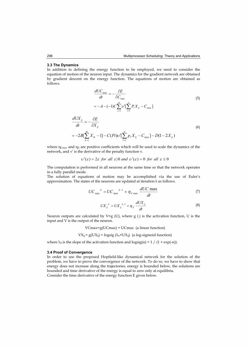
Multiprocessor Scheduling: Theory and Applications 298
3.3 The Dynamics
In addition to defining the energy function to be employed, we need to consider the equation of motion of the neuron input. The dynamics for the gradient network are obtained by gradient descent on the energy function. The equations of motion are obtained as follows.
m
j
n
iiji CXPCA
CE
dtdUC
1 1
max
max
max
][)1(
(5)
)21(][)(]1[21
max
1
ij
n
lljl
m
kik
ij
ij
XDCXpPiCXB
XE
dtdUX
(6)
where Cmax and X are positive coefficients which will be used to scale the dynamics of the network, and ’ is the derivative of the penalty function .
00)(02)( allforandallfor
The computation is performed in all neurons at the same time so that the network operates in a fully parallel mode. The solution of equations of motion may be accomplished via the use of Euler’s approximation. The states of the neurons are updated at iteration k as follows.
dtdUCUCUC C
kk maxmax
1
maxmax(7)
dtdUX
UXUX ijX
kij
kij
1 (8)
Neuron outputs are calculated by V=g (U), where g (.) is the activation function, U is the input and V is the output of the neuron.
VCmax=g(UCmax) = UCmax (a linear function)
VXij = g(UXij) = logsig ( X×UXij) (a log-sigmoid function)
where X is the slope of the activation function and logsig(n) = 1 / (1 + exp(-n)).
3.4 Proof of Convergence
In order to use the proposed Hopfield-like dynamical network for the solution of the problem, we have to prove the convergence of the network. To do so, we have to show that energy does not increase along the trajectories, energy is bounded below, the solutions are bounded and time derivative of the energy is equal to zero only at equilibria. Consider the time derivative of the energy function E given below.

Identical Parallel Machine Scheduling with Dynamical Networks using Time-Varying Penalty Parameters 299
1 1
1 1
1 1
2
max
max
max
max
max max
max
n mij
i j ij
n mij ij
i j
n mij ij
i j ij
ij ij
ij
VXdE E E VCdt VX dt VC dt
dUX dVX E VCdt dt VC dt
dVX dVXdUXij dUC dUCdt dVX dt dt dt
dVX dUX dVCdt dVX dt
2
1 1
n m
i j
(9)
Since 0])([ 1
ijij
ij VXgdVXdUX (monotone increasing) for log-sigmoid function, the right-
hand side of the equation given in (9) will be obviously negative. This ensures that the
energy does not increase along trajectories, so we can write 0dtdE .
0dtdE implies that jiallfor
dtdVX ij
,0 and 0max
dtdVC . In other words, 0
dtdE at
the equilibrium points. Since Xijs are binary variables, they are bounded but we have to check the boundedness of Cmax. If we rewrite the motion equation for Cmax, we obtain the following:
m
j
n
iiji VCVXPCA
VCE
dtdUC
1 1
max
max
max
][)1(
There may be different possible cases
Case 1: Assume that 0max
1
VCVXPn
iiji A
dtdUCmax
which means that UCmax=VCmax will decrease. This will cause
.0max
1
VCVXPn
iiji

Multiprocessor Scheduling: Theory and Applications 300
Case 2: Assume that 0max
1
VCVXPn
iiji A
dtdUCmax
which means that UCmax=VCmax will decrease. This will cause
0max
1
VCVXPn
iiji .
Therefore we have to consider Case 3 in which we assume 0max
1
VCVXPn
iiji
If 0max
1
VCVXPn
iiji
n
iiji
m
j
n
iiji
VXPCCVCA
VCVXPCA
VCE
dtdVC
dtdUC
1
max
1 1
max
max
maxmax
22
][)1(
Let r(z) ij
n
iiVXPCA
1
2
)(2 maxmax zrCVCdt
dVC
If we multiply both sides by eCt,
we get CtCtCt ezreCVC
dtdVC
e )(2 max
max
CtCt
CtCtCt
etrVCedtd
etreCVCdt
dVCe
)(][
)(2
max
maxmax

Identical Parallel Machine Scheduling with Dynamical Networks using Time-Varying Penalty Parameters 301
dzzreVCetVC
dzzreetVCd
tCzCt
tCz
etVC
eVC
Ct
Ct
C
)()0()(
)()).((
0
maxmax
0
)max(
)0max(
max.0
dzzreeVCetVC Czt
CtCt )()0()(0
maxmax
dzzreeVCe
dzzreeVCe
dzzreeVCetVC
dzzreeVCe
tCzCtCt
tCzCtCt
tCzCtCt
tCzCtCt
)()0(
)()0(
)()0()(
)()0(
0
max
0
max
0
maxmax
0
max
We can write
dzzreeVCe
dzzreeVCetVC
tCzCtCt
tCzCtCt
)()0(
)()0()(
0
max
0
maxmax
Assume that Mzr )(
]1[)0(
]1[1
)0(
)0()(
max
max
0
maxmax
CtCt
CtCtCt
tCzCtCt
ecMVCe
ec
MeVCe
dzeMeVCetVC

Multiprocessor Scheduling: Theory and Applications 302
Since 1Cte and as0Cte t , then
)(max tVC
n
iiji
n
iiji
n
iiji
ij
n
ii
VXPCA
VXPCA
VXPCAzr
VXPCAzr
1
1
1
1
2
2
2)(
2)(
Since A>0 and 021
n
iijiVXPC
)(zr and dt
dUCmax
and we can conclude that the solutions are bounded. Combining this fact with the fact that the energy E is bounded (since the cost is always greater than zero), we conclude that the network converges to a stable state which is a local minimum of E(X,Cmax). In other words, the time evolution of the network is a motion in space tends to that minimum point as t goes to infinity.
3.5 Selection of Parameters
In order to simulate the proposed network for solving the problem described by the dynamics given in Section 3.3, some parameters should be determined. These are the penalty parameters A, B, C and D; the activation slopes X; the step sizes Cmax, X and the initial conditions. Because there is no theoretically established method for choosing the values of the penalty coefficients for an arbitrary optimization problem, the appropriate values for these coefficients can be determined empirically. That is simulation runs are conducted, and optimality and/or feasibility of the resulting equilibrium points of the system are observed. The network can be initialized to small random values, and then synchronous or asynchronous updating of the network will allow a minimum energy state to be attained. In order to ensure smooth convergence, step size must be selected carefully (Watta & Hassoun, 1996). The dynamics of the proposed Hopfield-like gradient network will converge to local minima of the energy function E. Since the energy function includes four terms, competing to be minimized, there are many local minima and a tradeoff among the terms. An infeasible solution may be obtained when at least one of the constraint penalty terms is non-zero. In

Identical Parallel Machine Scheduling with Dynamical Networks using Time-Varying Penalty Parameters 303
this case, the objective function term will generally be quite small but the solution will not be feasible. Alternatively, a local minimum, which causes a feasible but not a good solution, may be encountered even if all the constraints are satisfied. In order to satisfy the each penalty term, its associated penalty parameter can be increased but this results an increase in other penalty terms and a tradeoff occurs. The penalty parameters that result a feasible and a good solution, which minimizes the objective function, should be found. Determining the appropriate values of the penalty parameters, network parameters and initial states are so critical issues associated with gradient type networks that by adjusting the parameters, the convergence performance to valid solutions can be improved. It is clear that solving scheduling problems represented by many constraints will cause a tradeoff among the penalty terms to be minimized.Due to the problems of Hopfield like NNs in solving optimization problems, various modifications are proposed to improve the convergence of the Hopfield network. While several authors modified the energy function of the Hopfield network to improve the convergence to valid solutions (Aiyer, Niranjan, & Fallside, 1990; Brandt, Wang, Laub & Mitra, 1988; Van Den Bout & Miller, 1988) many others studied the same formulation with different penalty parameters (Hedge, Sweet, & Levy, 1988; Kamgar-Parsi & Kamgar-Parsi, 1992; Lai & Coghill, 1992). In recent years, time based penalty parameters are proposed to overcome the tradeoff problems encountered in using penalty function approach. Wang (1991) used monotonically time-varying penalty parameters for solving convex programming problems. Dogan & Guzelis (2006) proposed linearly increasing time-varying penalty parameters for solving clustering problems. Here, we propose to use time varying penalty parameters that take zero values as a starting value and then are increased in a linear fashion in a stepwise manner to reduce the feasible region and also by updating all the neurons synchronously, better simulation results are obtained. The proposed gradient network algorithm can be summarised by the following pseudo-code.Step 1. Construct an energy function for the considered problem using a penalty function approach.Step 2. Initialize all neuron states to random values. Step 3. Select the slope of the activation function ( ) and step sizes ( ).Step 4. Determine penalty parameters
Step 4.1 Select C (the coefficient of the inequality constraint) and assign zero as initial value to other penalty parameters A, B and D. If the constraint associated with parameter C is satisfied, proceed to Step 4.2 otherwise go back to Step 4.1. Step 4.2 Select D (a higher value than C to increase the effect of equality constraint), and use the predetermined value of C (without taking into consideration of the effect of parameter A and B) to check whether both of the constraints associated with these terms are satisfied. If yes go to step 4.3, otherwise to step 4.4. Step 4.3. Select B (a higher value than D), assign 1 to A, and use the predetermined values of C, D together with B to check whether all of the constraints associated with these terms are satisfied. If yes go to step 5, otherwise to step 4.4. Step 4.4 Increase the value of parameter whose associated constraint is not satisfied.
Step 5. Repeat n times: Step 5.1. Update U using equations (7) and (8), and then compute V by V=g (U).
Step 6. If the energy has converged to local minimum proceed to step 7, otherwise go back to step 5.

Multiprocessor Scheduling: Theory and Applications 304
Step 7. Examine the final solution to determine feasibility and optimality. Step 8. Adjust parameters A, B, C, D if necessary to obtain a satisfactory solution, reinitialize neuron states and repeat from step 5.
3.6 An Example
We explain the procedure with a 5-job 3-machine identical parallel machine scheduling problem. After constructing the energy function for this problem, all neuron states are initialized to random values chosen uniformly from the interval [0,1]. In the proposed approach, we firstly suggest to satisfy the inequality constraint by penalizing it. In the first phase of the simulation (for the first 2000 iterations), initial value of the penalty parameter C is chosen as 8. Because other penalty parameters are not taken into consideration, they are equal to zero. Since this inequality constraint is satisfied after 2000 iterations, it is decided to proceed to the next phase. In the second phase (for iterations from 2001 to 4000), one of the equality constraints (binary constraints) is taken into consideration, and its associated parameter D is chosen as 20, a value greater than C. The predetermined value of C, 8, is used to penalize the inequality constraint. Both of the constraints are satisfied. Thus, it is decided to proceed to the next phase (for iterations from 4001 to 5000). In this phase, all of the constraints are tried to be satisfied. Together with the predetermined values of C and D, the penalty parameter B belonging to the assignment constraint is chosen as 100 (a value greater than other parameters). Since A belongs to the original objective function, it is not penalized, and we assign 1 to A. After running simulations with all these 4 penalty terms, the feasibility and optimality of the final solution is checked. It is seen that except the inequality constraint, being violated with a small percentage error, all of the constraints are satisfied. Therefore, it is decided to enhance the weight of this constraint, and then value of its parameter, C, is increased to 600. Optimal solution is found at iteration 5100. All of the constraints were met satisfactorily, and the cost value is 3.1. In Table 1, values of penalty parameters used during the solution of the problem considered are displayed.
Penalty Coef.
Iterations
A B C D
1:2000 0 0 8 0
2001:4000 0 0 8 20
4001:5000 1 100 8 20
5001:5100 1 1 600 1
Table 1. Penalty parameter values in four phases of simulation
4. Simulation Results
A simulation experiment was conducted to test the effectiveness of the proposed gradient network approach in terms of solution quality. The initial conditions of the network and the processing times of jobs were chosen randomly from uniform distribution in an interval [0,1], and [1,3], respectively. In tables 2-11, penalty coefficients of the proposed gradient network and other parameters which were determined empirically by running trial simulations are given.
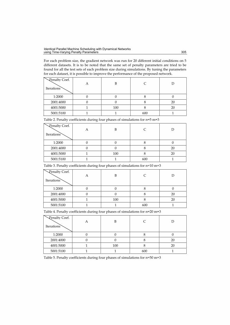
Identical Parallel Machine Scheduling with Dynamical Networks using Time-Varying Penalty Parameters 305
For each problem size, the gradient network was run for 20 different initial conditions on 5 different datasets. It is to be noted that the same set of penalty parameters are tried to be found for all the test sets of each problem size during simulations. By tuning the parameters for each dataset, it is possible to improve the performance of the proposed network.
Penalty Coef.
Iterations
A B C D
1:2000 0 0 8 0
2001:4000 0 0 8 20
4001:5000 1 100 8 20
5001:5100 1 1 600 1
Table 2. Penalty coefficients during four phases of simulations for n=5 m=3
Penalty Coef.
Iterations
A B C D
1:2000 0 0 8 0
2001:4000 0 0 8 20
4001:5000 1 100 8 20
5001:5100 1 1 600 1
Table 3. Penalty coefficients during four phases of simulations for n=10 m=3
Penalty Coef.
Iterations
A B C D
1:2000 0 0 8 0
2001:4000 0 0 8 20
4001:5000 1 100 8 20
5001:5100 1 1 600 1
Table 4. Penalty coefficients during four phases of simulations for n=20 m=3
Penalty Coef.
Iterations
A B C D
1:2000 0 0 8 0
2001:4000 0 0 8 20
4001:5000 1 100 8 20
5001:5100 1 1 600 1
Table 5. Penalty coefficients during four phases of simulations for n=50 m=3

Multiprocessor Scheduling: Theory and Applications 306
Penalty Coef.
Iterations
A B C D
1:2000 0 0 8 0
2001:4000 0 0 8 20
4001:5000 1 100 8 20
5001:5100 1 1 600 1
Table 6. Penalty coefficients during four phases of simulations for n=100 m=3
Penalty Coef.
Iterations
A B C D
1:2000 0 0 8 0
2001:4000 0 0 8 20
4001:5000 1 100 8 20
5001:5100 1 1 600 1
Table 7. Penalty coefficients during four phases of simulations for n=10 m=5
Penalty Coef.
Iterations
A B C D
1:2000 0 0 10 0
2001:4000 0 0 10 30
4001:5000 1 100 10 30
5001:5100 1 1 600 1
Table 8. Penalty coefficients during four phases of simulations for n=20 m=5
Penalty Coef.
Iterations
A B C D
1:2000 0 0 10 0
2001:4000 0 0 10 30
4001:5000 1 100 10 30
5001:5100 1 1 600 1
Table 9. Penalty coefficients during four phases of simulations for n=50 m=5
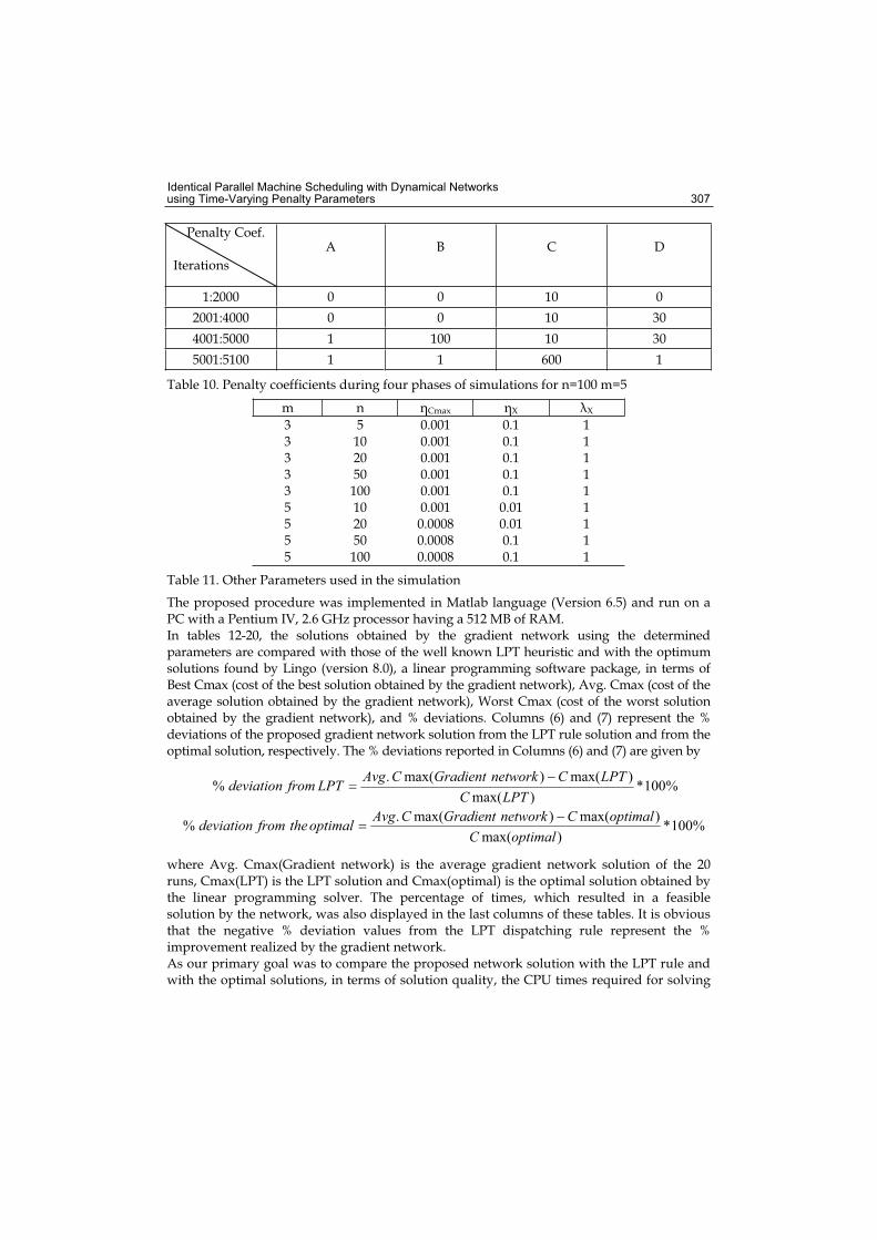
Identical Parallel Machine Scheduling with Dynamical Networks using Time-Varying Penalty Parameters 307
Penalty Coef.
Iterations
A B C D
1:2000 0 0 10 0
2001:4000 0 0 10 30
4001:5000 1 100 10 30
5001:5100 1 1 600 1
Table 10. Penalty coefficients during four phases of simulations for n=100 m=5
m n Cmax X X
3 5 0.001 0.1 13 10 0.001 0.1 13 20 0.001 0.1 13 50 0.001 0.1 13 100 0.001 0.1 15 10 0.001 0.01 15 20 0.0008 0.01 15 50 0.0008 0.1 15 100 0.0008 0.1 1
Table 11. Other Parameters used in the simulation
The proposed procedure was implemented in Matlab language (Version 6.5) and run on a PC with a Pentium IV, 2.6 GHz processor having a 512 MB of RAM. In tables 12-20, the solutions obtained by the gradient network using the determined parameters are compared with those of the well known LPT heuristic and with the optimum solutions found by Lingo (version 8.0), a linear programming software package, in terms of Best Cmax (cost of the best solution obtained by the gradient network), Avg. Cmax (cost of the average solution obtained by the gradient network), Worst Cmax (cost of the worst solution obtained by the gradient network), and % deviations. Columns (6) and (7) represent the % deviations of the proposed gradient network solution from the LPT rule solution and from the optimal solution, respectively. The % deviations reported in Columns (6) and (7) are given by
%100*)max(
)max()max(.%
LPTCLPTCnetworkGradientCAvgLPTfromdeviation
%100*)max(
)max()max(.%
optimalCoptimalCnetworkGradientCAvgoptimalthefromdeviation
where Avg. Cmax(Gradient network) is the average gradient network solution of the 20 runs, Cmax(LPT) is the LPT solution and Cmax(optimal) is the optimal solution obtained by the linear programming solver. The percentage of times, which resulted in a feasible solution by the network, was also displayed in the last columns of these tables. It is obvious that the negative % deviation values from the LPT dispatching rule represent the % improvement realized by the gradient network. As our primary goal was to compare the proposed network solution with the LPT rule and with the optimal solutions, in terms of solution quality, the CPU times required for solving

Multiprocessor Scheduling: Theory and Applications 308
each data set are not given. But from the simulation experiments, it is seen that when compared with the very long solution times needed to obtain the optimal solutions by the Lingo software, the proposed network could converge to valid solutions in reasonable times between 13.18 seconds (for n=3 m=5) and 203.57 seconds (for n=100 m=5). Obviously, by the implementation of the proposed network in a dedicated hardware, significant reductions can be obtained in running times.
Gradient Network
Best Cmax
(1)
Avg.Cmax
(2)
WorstCmax
(3)
LPT(4)
Optimum(5)
Deviation (%) from the LPT solution
(6)
Deviation(%) from
theoptimalsolution
(7)
PercentFeasibility
ofComputedSolutions
(8)
3.1 3.1 3.1 3.1 3.1 0.00 0.00 100%
4.69 4.69 4.69 4.69 4.69 0.00 0.00 100%
3.55 3.55 3.55 3.55 3.55 0.00 0.00 100%
2.98 2.98 2.98 2.98 2.98 0.00 0.00 100%
3.02 3.02 3.02 3.02 3.02 0.00 0.00 100%
Table 12. Results for m=3, n=5 over 5 problems
Gradient Network
Best Cmax
(1)
Avg.Cmax
(2)
WorstCmax
(3)
LPT(4)
Optimum(5)
Deviation (%) from the LPT solution
(6)
Deviation (%) from
theoptimalsolution
(7)
PercentFeasibility
ofComputedSolutions
(8)
7.33 7.54 7.67 7.59 7.21 -0.66 4.57 100 %
6.97 7.21 7.47 7.45 6.92 -3.22 4.19 100 %
7.28 7.56 7.72 7.69 7.2 -1.69 5 100 %
6.79 7.11 7.30 7.46 6.72 -4.69 5.80 100 %
6.77 7.01 7.31 7.44 6.72 -5.78 4.31 100 %
Table 13. Results for m=3, n=10 over 5 problems

Identical Parallel Machine Scheduling with Dynamical Networks using Time-Varying Penalty Parameters 309
Gradient Network
Best Cmax
(1)
Avg.Cmax
(2)
WorstCmax
(3)
LPT(4)
Optimum(5)
Deviation(%) from the LPT solution
(6)
Deviation (%) from
theoptimalsolution
(7)
PercentFeasibility
ofComputedSolutions
(8)
13.24 13.53 13.85 13.37 13.05 1.19 3.68 100 %
13.84 14.24 14.46 14.01 13.74 1.64 3.64 100 %
13.03 13.42 13.63 13.40 12.92 0.15 3.87 100 %
14.25 14.54 14.76 14.60 14.05 -0.41 3.48 100 %
13.35 13.60 13.82 13.46 13.12 1.04 3.66 100 %
Table 14. Results for m=3, n=20 over 5 problems
Gradient Network
Best Cmax
(1)
Avg.Cmax
(2)
WorstCmax
(3)
LPT(4)
Optimum(5)
Deviation(%) from the LPT solution
(6)
Deviation (%) from
theoptimalsolution
(7)
PercentFeasibility
ofComputedSolutions
(8)
33.53 33.84 34.07 33.70 33.34 0.41 1.50 100 %
30.58 30.95 31.14 30.75 30.36 0.65 1.94 100 %
31.47 31.85 32.15 31.65 31.38 0.63 1.49 100 %
34.53 35.41 35.77 35.32 34.92 0.25 1.40 100 %
34.68 35.10 35.30 34.88 34.51 0.63 1.71 100 %
Table 15. Results for m=3, n=50 over 5 problems
Gradient Network
Best Cmax
(1)
Avg.Cmax
(2)
WorstCmax
(3)
LPT(4)
Optimum(5)
Deviation(%) from the LPT solution
(6)
Deviation (%) from
theoptimalsolution
(7)
PercentFeasibility
ofComputedSolutions
(8)
70.00 70.28 70.58 70.55 69.91 -0.38 0.53 100 %
66.65 66.94 67.14 67.09 66.45 -0.22 0.73 100 %
68.42 68.85 69.10 69.04 68.39 -0.27 0.67 100 %
66.11 66.73 66.52 66.73 66.09 0.00 0.97 100 %
65.85 66.15 66.33 66.35 65.69 -0.30 0.70 100 %
Table 16. Results for m=3, n=100 over 5 problems

Multiprocessor Scheduling: Theory and Applications 310
Gradient Network
Best Cmax
(1)
Avg.Cmax
(2)
WorstCmax
(3)
LPT(4)
Optimum(5)
Deviation(%) from the LPT solution
(6)
Deviation(%) from the
optimalsolution
(7)
PercentFeasibility
ofComputedSolutions
(8)
3.43 3.53 3.68 3.43 3.43 2.91 2.91 100 %
3.38 3.76 3.97 3.79 3.38 -0.79 11.24 100 %
3.64 3.85 3.97 3.68 3.57 4.35 7.56 100 %
4.03 4.16 4.24 4.03 4.03 3.22 3.22 100 %
3.57 3.67 3.73 3.53 3.53 3.97 3.97 100 %
Table 17. Results for m=5, n=10 over 5 problems
Gradient Network
Best Cmax
(1)
Avg.Cmax
(2)
WorstCmax
(3)
LPT(4)
Optimum(5)
Deviation(%) from the LPT solution
(6)
Deviation (%) from
theoptimalsolution
(7)
PercentFeasibility
ofComputedSolutions
(8)
7.43 7.78 7.91 7.37 7.28 5.56 6.87 100 %
7.68 7.95 8.08 7.62 7.49 4.33 6.14 100 %
8.13 8.24 8.37 7.8 7.76 5.64 6.18 100 %
7.79 7.98 8.13 7.69 7.51 3.77 6.26 100 %
8.55 8.77 8.92 8.29 8.18 5.79 7.21 100 %
Table 18. Results for m=5, n=20 over 5 problems
Gradient Network
Best Cmax
(1)
Avg.Cmax
(2)
WorstCmax
(3)
LPT(4)
Optimum(5)
Deviation(%) from the LPT solution
(6)
Deviation (%) from
theoptimalsolution
(7)
PercentFeasibility
ofComputedSolutions
(8)
20.49 20.86 21.09 20.28 20.22 2. 86 3.16 100 %
21.70 22.17 22.42 21.55 21.49 2.88 3.16 100 %
18.69 18.94 19.15 18.42 18.40 2.82 2.93 100 %
20.71 21.11 21.33 20.37 20.33 3.63 3.83 100 %
19.79 20.01 20.24 19.43 19.41 2.98 3.09 100 %
Table 19 Results for m=5, n=50 over 5 problems

Identical Parallel Machine Scheduling with Dynamical Networks using Time-Varying Penalty Parameters 311
Gradient Network
Best Cmax
(1)
Avg.Cmax
(2)
WorstCmax
(3)
LPT(4)
Optimum(5)
Deviation(%) from the LPT solution
(6)
Deviation (%) from
theoptimalsolution
(7)
PercentFeasibility
ofComputedSolutions
(8)
41.65 41.87 42.06 41.24 41.20 1.53 1.63 100 %
40.16 40.56 40.74 39.78 39.77 1.96 1.99 100 %
41.90 42.12 42.28 41.36 41.34 1.84 1.89 100 %
40.20 40.55 40.69 39.83 39.82 1.80 1.83 100 %
41.54 41.89 42.06 41.19 41.15 1.70 1.8 100 %
Table 20. Results for m=5, n=100 over 5 problems
To interpret the findings in a table, let us consider Table 12. For all the 5 data sets, 20 out of the 20 runs of the proposed network resulted in a feasible solution, that is percent feasibility is 100 %. The average, worst and the best cost of the 20 feasible solutions for the first dataset is 3.1, which is equal to the global optimal solution value, therefore the percent above the optimal solution and LPT result is 0.0. Similarly, if we consider Table 20, for the first dataset, again, 100 % of the runs resulted in a feasible solution by the proposed network. The average Cmax of the feasible solutions is 41.87, which is 1.53 % more costly than the result of LPT rule, and 1.63 % more costly than the global optimal solution. The best makespan value produced by the gradient network is 41.65, which is 0.99 % ([(41.65-41.24)*100]/41.24) above than the LPT result and 1.09 % ([(41.65-41.20)*100]/41.20) above the global optimal solution. According to these findings, it is clear that the initial conditions of the network appear to have a serious impact on the solution quality. For example in Table 17, for n=10 and m=5, although the proposed network results in gaps between 2.91 and 4.35 % from the LPT solution, on average, it outperforms the LPT heuristic for one of the datasets. In the same table, if the results obtained using the first data set are considered, it is seen that although the average makespan from the 20 different initial runs is found as 3.53, the best makespan out of the 20 runs, produced by the proposed network is 3.43, which is equal to the optimal solution. In addition, although the average Cmax results obtained by the proposed network are above the LPT results for the 4 data sets, the best Cmax results outperform the LPT rule in 4 data sets. In all the simulations carried out to show the performance of the network, convergence to valid schedules is achieved and better results are obtained for small number of machines and large number of jobs. If all the test cases are considered, the proposed network is, on average, able to produce a solution with a makespan value, which is 1.14 % above of cost of the LPT result. By tuning the penalty coefficients for each dataset, it is possible to improve the convergence and the optimality of the solutions. On the other hand, besides its convergence to valid schedules, convergence to good quality solutions of the proposed network points out its general applicability in other scheduling environments.

Multiprocessor Scheduling: Theory and Applications 312
5. Conclusions and Future Research
This study has presented a dynamical gradient network for solving the identical parallel machine scheduling problem with the makespan criterion which is known to be NP-hard even for the case of two identical parallel machines. Focus of this paper has been on demonstrating the optimization capabilities of the proposed network by solving a set of randomly generated problems. The proposed Hopfield-like network uses time-varying penalty parameters that start from zero and increase in a stepwise manner during iterations to overcome the tradeoff problem of the penalty function method, one of the important drawbacks of the penalty function approach.. To analyse the performance of the network, it is compared with the well-known LPT heuristic commonly used to solve the problem under study, and also with the optimal solutions in terms of the solution quality. The simulation experiments demonstrated that the proposed network generated feasible solutions in all the cases, and, in some of the data sets it found smaller makespan compared to LPT. In general, for all the instances, the average deviation percentage of the proposed network is 1.14 % from the LPT heuristic. By conducting several simulation experiments, the influence of different initializations schemes was investigated on the solutions of the problem considered. The analysis results showed that the percent error of the network is very sensitive to the selection of the starting points and the choice of the parameters used in simulation. The contribution of this paper is two fold. We propose to use a novel time varying penalty method that guarantees feasible and near optimal solutions for solving the identical parallel machine scheduling problem with the makespan criterion. Although a large body of literature exists for solving identical parallel machine scheduling problem with the makespan minimization criterion, to the best of our knowledge, there is no previously published article that tried to solve this NP-hard problem using neural networks, so that this study will also make a contribution to the scheduling literature. Several issues are worthy of future investigations. First, further studies will be focused on selecting the parameters of the network automatically rather than choosing by trial and error, which is one of the drawbacks of neural networks. Second, extension of the results to large size problems will be worthwhile. Finally, extension of the results to different manufacturing scheduling environments is important for industrial applications, and implementation of the network in hardware can make progress in computational efficiency.
6. References
Aiyer, S.V.B.; Niranjan, M. & Fallside, F. (1990). A theoretical investigation into the performance of the Hopfield model. IEEE Transactions on Neural Networks. 1, 204-215.
Akyol, D.E. & Bayhan, G.M. (2005). A Coupled Gradient Network Approach for the Multi Machine Earliness and Tardiness Scheduling Problem, Lecture notes in computer science, 3483, 596-605.
Akyol, D.E. & Bayhan, G.M. (2006). Minimizing Makespan on Identical Parallel Machines using Neural Networks, Lecture notes in computer science, 4234, 553-562.
Brandt, R.D.; Wang, Y.; Laub, A.J. & Mitra. S.K. (1988). Alternative Networks for Solving the Travelling Salesman Problem and the List-Matching Problem. In Proceedings of the International Conference on Neural Networks, 2, 333-340.

Identical Parallel Machine Scheduling with Dynamical Networks using Time-Varying Penalty Parameters 313
Chen, M. & Dong, Y. (1999). Applications of neural networks to solving SMT scheduling problems-a case study. International Journal of Production Research, 37, 4007-4020.
Cheng, T. & Sin, C. (1990). A State-of-the-Art Review of Parallel-Machine Scheduling Research. European Journal of Operational Research, 47, 271-292.
Coffman, E.G., Garey, M.R. & Johnson, D.S. (1978). An application of bin-packing to multi-processor scheduling, SIAM Journal of Computing, 7, 1-17.
Dogan, H. & Guzelis, C. (2006). Robust and Fuzzy Spherical Clustering by a Penalty Parameter Approach. IEEE Transactions on Circuits and Systems-II. 53(8), 637-641.
Foo, S.Y.; Takefuji, Y. & Szu, H. (1995). Scaling properties of neural networks for job-shop scheduling, Neurocomputing, 8, 79-91.
Frangioni, A.; Scutella, M.G. & Necciari, E. (1999). Multi-exchange algorithms for the minimum makespan machine scheduling problem, Technical Report: TR-99-22.
Friesen, D.K. & Langston, M.A. (1986). Evaluation of a MULTIFIT based scheduling algorithm, J. Algorithm, 7, 35-59.
Friesen, D.K. (1987). Tighter bounds for LPT scheduling on uniform processors. SIAM J. Computing. 16, 554-560.
Garey, M.R. & Johnson, D.S. (1979). Computer and intractability: a guide to the theory of NP completeness, (W.H Freeman, San Francisco).
Graham, R.L. (1969). Bounds on multiprocessor timing anomalies. SIAM Journal of Applied Mathematics, 17, 416-429.
Graham, R.L.; Lawler, E.L.; Lenstra, J.K. & Rinnooy Kan, A.H.G. (1979). Optimization and approximation in deterministic sequencing and scheduling: A survey. Annals of Discrete Mathematics, 5, 287–326.
Hamad, A.; Sanugi, B. & Salleh, S. (2003). A neural network model for the common due date job scheduling on unrelated parallel machines, International Journal of Computer Mathematics, 80, 845-851.
Hedge, S.; Sweet, J. & Levy, W. (1988). Determination of parameters in a Hopfield/Tank computational network. In Proc. IEEE International Conference on Neural Networks, 2, 291-298.
Hochbaum, D.S. & Shmoys, D.B. (1987). Using dual approximation algorithms for scheduling problems: Practical and theoretical results. Journal of the Association for Computing Machinery. 34, 144-162.
Hopfield, J. (1984). Neurons with graded response have collective computational properties like of two-state neurons. In Proc. of the National Academy of Sciences of the USA, 81, 3088-3092.
Hopfield, J. & Tank, T.W. (1985). Neural computation of decisions in optimization problems. Biological Cybernetics, 52, 141-152.
Hübscher, R. & Glover, F. (1994). Applying Tabu Search with influential diversification to multiprocessor scheduling, Computers and Operations Research, 8, 877-884.
Jozefowska, J.; Milka, M.; Rozycki, R.; Waligora, G. & Weglarz, J. (1998). Local search metaheuristics for discrete-continuous problems. European Journal of Operational Research, 107, 354-370.
Kamgar-Parsi, B. & Kamgar-Parsi, B. (1992). Dynamical Stability and Parameter Selection in Neural Optimization. Proc. of International Joint Conference on Neural Networks, 4, 566-571.

Multiprocessor Scheduling: Theory and Applications 314
Lai, W.K. & Coghill, G.G. (1992). Genetic Breeding of Control Parameters for the Hopfield/Tank Neural Net. Proc. of the International Joint Conference on Neural Networks, 4, 618-623.
Leung, J.Y.-T. (1989). Bin packing with restricted piece sizes, Information Processing Letters,31, 145-149.
Liansheng, G.; Gang, S. & Shuchun, W. (2000). Intelligent scheduling model and algorithm for manufacturing, Production Planning and Control, 11, 234-243.
Lo, Z.P. & Bavarian, B. (1993). Multiple job scheduling with artificial neural networks. Computers and Electrical Engineering, 19, 87-101.
Mokotoff, E. (2001). Parallel Machine Scheduling Problems: A Survey. Asia-Pacific Journal of Operational Research, 18, 193-242.
Park, Y.; Kim, S. & Lee, Y.H. (2000). Scheduling jobs on parallel machines applying neural network and heuristic rules. Computers and Industrial Engineering, 38, 189-202.
Sahni, S.K. (1976). Algorithms for scheduling independent tasks. J. Assoc. Comput mach., 23, 116-127.
Satake, T.; Morikawa, K. & Nakamura, N. (1994). Neural network approach for minimizing the makespan of the general job-shop. International Journal of Production Economics.33, 67-74.
Sethi, R. (1977). On the complexity of mean flow time scheduling. Mathematics of Operations Research. 2, 320-330.
Vaithyanathan, S. & Ignizio, J.P. (1992). A stochastic neural network for resource constrained scheduling. Computers and Operations Research, 19, 241-254.
Van Den Bout, D.E. & Miller, T.K. (1988). A Traveling Salesman Objective Function that Works. In Proc. of IEEE International Conference on Neural Networks, 2, 299-303.
Wang, J. (1991). A Time-Varying Recurrent Neural System for Convex Programming. Proc.of IJCNN-91-Seattle International Joint Conference on Neural Networks, 147-152.
Watta, P.B. & Hassoun, M.H. (1996). A Coupled Gradient Network Approach for Static and Temporal Mixed-Integer Optimization. IEEE Transactions on Neural Networks, 7, 578-593.
Willems, T.M. & Brandts, E.M.W. (1995). Implementing heuristics as an optimization criterion in neural networks for job-shop scheduling. Journal of Intelligent Manufacturing, 6, 377-387.
Zhou, D.N.; Cherkassy, V.; Baldwin, T.R. & Olson, D.E. (1991). A Neural Network Approach to Job-Shop Scheduling. IEEE Transactions on Neural Networks, 2, 175-179.

18
A Heuristic Rule-Based Approach for Dynamic Scheduling of Flexible Manufacturing Systems
Gonca Tuncel Dokuz Eylul University, Department of Industrial Engineering, Izmir
Turkey
1. Introduction
Operations planning and scheduling (OPS) problems in flexible manufacturing systems (FMSs), are composed of a set of interrelated problems, such as part-type batching, machine grouping, part routing, tool loading, part input sequencing, and resource assignment. The performance of an FMS is highly dependent on the efficient allocation of the limited resources to the tasks, and it is strongly affected by the effective choice of scheduling rules. In this study, a heuristic ruled based approach for dynamic scheduling of FMSs, which integrates loading, part inputting, routing, and dispatching issues of the OPS is presented, and the implementation results are compared with several dispatching rules. Scheduling is a decision making process and it concerns the allocation of the limited resources to tasks over time [1]. In a manufacturing system, resources represent machines, operators, robots, tools, buffers etc., and activities are the processing of products on machines, the transportation of products among workstations, or loading/unloading the parts from/to machines by the operators. The scheduling problems in FMSs, relate to the execution of production orders and include raw part input sequencing, machine, material handling device and operator scheduling, part routing, monitoring the system performance and taking the necessary corrective actions [2]. Since FMSs comprise very diverse properties and constraints (e.g. the availability of alternative machines to perform the same operation(s), multi-layer resource sharing, and product varieties), scheduling problems in FMSs are more complex than job-shop or flow-shop problems and often very difficult to be solved by conventional optimization techniques. Prior studies on FMS scheduling problem point out the great impact of scheduling decisions to the system performance [3-5]. Scheduling decisions and the effective choice of dispatching rules are influenced by the performance criterion and existing shop-floor conditions such as process plans, due date requirements, release dates, job priorities, machine setup requirements, and the availability of system resources. Scheduling/dispatching control decisions in an FMS must be capable of handling simultaneously these diverse factors on a real-time basis. Therefore, rather than designing an optimum scheduler, there is a definitive need for a flexible and integrated scheduling in order to handle the dynamic and stochastic nature of real-world problems, and computationally efficient compared to analytical methods. In this study, a heuristic rule-based approach is proposed to solve the resource contention problem in an FMS, and to determine the best route(s) of the parts, which have routing

Multiprocessor Scheduling: Theory and Applications 316
flexibility. The paper is organized as follows. Section 2 describes the resource contention problem considered in this study. The proposed heuristic rule based system is presented in the following section. In section 4, the dynamic scheduling methodology is illustrated on an example FMS, and the performance of the proposed rule-based system is compared with single dispatching rules. Finally, conclusions and future research directions are given in the last section.
2. Problem Statement
Due to the unavailability of sufficiently large problem sets, the researchers studying on FMSs mostly generate their specific systems [6]. In this study, an FMS with alternative operations and setup times is employed to explain the proposed decision support system for dynamic shop-floor scheduling and control problem. The FMS operational policy is under push paradigm that machines process parts whenever they are available. Some operations of the product types can be performed by alternative machines. From the point of part flow view three different types of products are processed simultaneously in the system, and each product is allowed to have flexible routing (i.e. two or more machines have the ability to perform the same operation of a part). Employing flexible routing requires a two-level hierarchical decision making process: assignment and sequencing. In the first level, the next destination of a job is determined; in the second level the sequencing decisions of a part waiting for the limited resources such as workstations, operators, and transporter is taken. For scheduling of automated manufacturing systems, supplementary resources such as material handling system, operators and buffer spaces should also be taken into consideration while taking scheduling decisions. However, this will increase the problem complexity, since deadlocks may arise from distinct recognition of multilayer resource sharing. In the system considered, when the part type is changed, a setup operation is needed. Therefore, we also have to introduce setup requirements of the machines into the rule-based system while solving the conflict problems. In order to achieve the efficient utilization of the resources, and to find out the best operation sequence of each task, a real-time resource allocation policy is needed to be adapted, thus to assign resources to the jobs as they advance through the system. Moreover, the scheduling decisions should consider the prevailing conditions of the shop-floor in an integrated framework. Since a variety of part types have alternative routes on the machines, and multiple resources can be selected in a given set, a conflict or deadlock may often arise when more than one part is contesting for the same resources such as machines, material handling devices, and operators. Thus, the problem is the allocation of limited resources to a set of tasks, that is determination of the best route of each task in the system according to the current shop-floor condition (i.e. due dates, release dates, order quantities, tardiness penalties, inventory levels, priorities, and setup times). However, formulation of real-life scheduling problem using traditional methods becomes very complex when part routing flexibility, machine setup operations, operator and material handling system constraints are also considered.
3. A Heuristic Rule-Based System for Dynamic Scheduling
The system control and scheduling approach in the proposed methodology uses a heuristic rule-based system to solve resource contention problems and to determine the best route(s)

A Heuristic Rule-Based Approach for Dynamic Scheduling of Flexible Manufacturing Systems 317
of the parts, which have routing flexibility. The part routing control system aims to handle material handling, operator and setup operation constraints together with the machine constraints, thus to solve both sequencing and resource sharing problem effectively at the same time. The proposed approach is modeled with the help of the high-level Petri Net (PN) model of the system by the sequence of execution of transitions [7]. PNs, as a graphical and mathematical modeling tool, are well suited for representing FMS characteristics such as precedence relations, concurrency, conflicts, and synchronization [8-9]. In the developed scheduling system, part flow between workstations are controlled and managed by a scheduler module. All the information of each part which is ready to be transported in the system is sent to the scheduler module. In the scheduler module, the next destination of a part is determined dynamically based on the existing shop-floor conditions and the proposed heuristics, then sends a request for AGV assignment. The Scheduler module examines the system state at every discrete event when there is a change in the status of the system and makes a decision applying scheduling rules in the knowledge base then passes the decision to the system. Thus, it provides a computerized support to the user so that the decision is taken after comparing the different available options of scheduling which are better in respect to the different aspects such as due dates, overhead costs, minimum tardiness, and flow time. A set of production rules in the form of "IF..... THEN....." statements have been constructed based on the heuristics developed for this work to assign the resources to the parts, and to determine the best route(s) of the parts thus to solve the resource contention problem. A production rule which is a means of expressing reasoning links between facts expresses the behavior of objects in the system of interest [10].
where, the cj (j =1,2,..., m) are predicates known as conditions, and the rk (k = 1,2,..., n) are to as consequences. A predicate checks the state of the system, such as the process plan of the parts, the number of conflicting part types, their remaining number of operations, their remaining process times, and the setup status of the machines, then selects the next part to be processed from a set of parts awaiting according to some priority rules. When the IF portion of a production rule (predicate) is satisfied by the conditions, the action specified by the THEN portion is performed. When this happens, the rule is said to be fired. In scheduler module, a rule interpreter compares the IF portion of each rule with the facts and executes the rules whose IF portions match the facts. Each rule in this scheme corresponds to the use of a routing control strategy subject to the existence of certain conditions. Instead of using a single dispatching rule, it is more expedient to apply one from a set of dispatching rules according to the decision point and system characteristics. In the IF...-THEN... statements, the following dispatching procedural rules are used in decision making process;
First come, first served, (FCFS or FIFO) Earliest due date, (EDD) Smallest number of remaining operations, (SNRO) Largest number of remaining operations, (LNRO) Shortest processing time, (SPT) Job of identical setup, (JIS) Critical Ratio scheduling, (CR)

Multiprocessor Scheduling: Theory and Applications 318
Figure 1. Flow Chart of the Routing Control Process
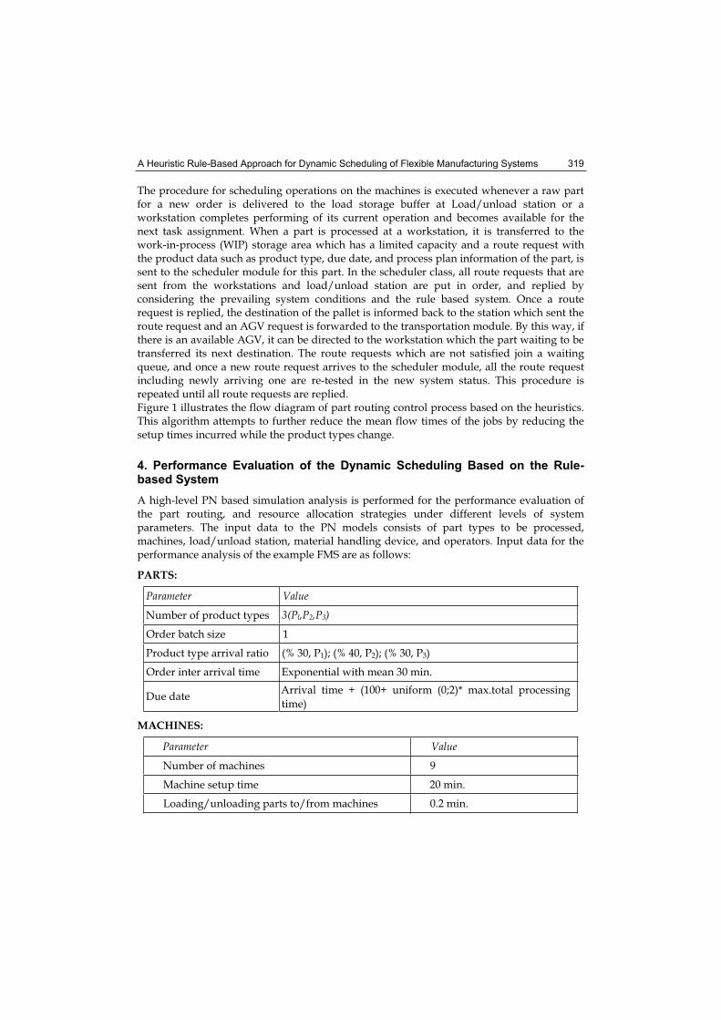
A Heuristic Rule-Based Approach for Dynamic Scheduling of Flexible Manufacturing Systems 319
The procedure for scheduling operations on the machines is executed whenever a raw part for a new order is delivered to the load storage buffer at Load/unload station or a workstation completes performing of its current operation and becomes available for the next task assignment. When a part is processed at a workstation, it is transferred to the work-in-process (WIP) storage area which has a limited capacity and a route request with the product data such as product type, due date, and process plan information of the part, is sent to the scheduler module for this part. In the scheduler class, all route requests that are sent from the workstations and load/unload station are put in order, and replied by considering the prevailing system conditions and the rule based system. Once a route request is replied, the destination of the pallet is informed back to the station which sent the route request and an AGV request is forwarded to the transportation module. By this way, if there is an available AGV, it can be directed to the workstation which the part waiting to be transferred its next destination. The route requests which are not satisfied join a waiting queue, and once a new route request arrives to the scheduler module, all the route request including newly arriving one are re-tested in the new system status. This procedure is repeated until all route requests are replied. Figure 1 illustrates the flow diagram of part routing control process based on the heuristics. This algorithm attempts to further reduce the mean flow times of the jobs by reducing the setup times incurred while the product types change.
4. Performance Evaluation of the Dynamic Scheduling Based on the Rule-based System
A high-level PN based simulation analysis is performed for the performance evaluation of the part routing, and resource allocation strategies under different levels of system parameters. The input data to the PN models consists of part types to be processed, machines, load/unload station, material handling device, and operators. Input data for the performance analysis of the example FMS are as follows:
PARTS:
Parameter Value
Number of product types 3(Pl,P2,P3)
Order batch size 1
Product type arrival ratio (% 30, P1); (% 40, P2); (% 30, P3)
Order inter arrival time Exponential with mean 30 min.
Due date Arrival time + (100+ uniform (0;2)* max.total processing
time)
MACHINES:
Parameter Value
Number of machines 9
Machine setup time 20 min.
Loading/unloading parts to/from machines 0.2 min.

Multiprocessor Scheduling: Theory and Applications 320
LOAD/ UNLOAD PROCESS:
Parameter Value
Loading / unloading parts to/from pallets 0.3 min.
Moving pallets to load / unload storage buffers 0.2 min.
MATERIAL HANDLING SYSTEM:
Parameter Value
Number of AGVs 1
Transfer time between the stations 1.5 min.
OPERATORS:
Parameter Value
Number of operators 8
Operator transfer time between workstations 0.5 min
For each product type, Tables 1 and 2 show the operational sequences with required resources and processing times without setup times.
Operations Machine required - Processing time
O-l M-l (4.5 min.) / M-3 (3.2 min.)
O-2 M-2 (4.5 min.) / M-4 (3.2 min.)
O-3 M-5 (9 min.) / M-6 (5.2 min.) / M-7 (6 min.) / M-3 (3.6 min.)
O-4 M-8 (2 min.)
O-5 M-9(1.5min.)
Table 1. Process plan of product type 1 (P1)
Operations Machine required - Processing time
O-l M-3 (3.7 min)
O-2 M-4 (5.3 min.)
O-3 M-5 (13 min.) / M-6 (7.5 min. for P2; 8.5 min. for P3) / M-3 (5.25 min.)
O-4 M-8 (2 min.)
O-5 M-9(1.5min.)
Table 2. Process plan of product type 2 and 3 (P2 and P3)
Ten independent replications for each dispatching strategies were run for 180.000 operating minutes (125 days with three 8 hr shifts) during the simulation of the PN model. In each run, the shop is continuously loaded with job-orders that are numbered on arrival, and each run produced one observation for each performance measure. Different random number seeds were used to prevent correlation between the parallel runs of the factorial experiment. In

A Heuristic Rule-Based Approach for Dynamic Scheduling of Flexible Manufacturing Systems 321
order to ascertain when the system reaches a steady state, the shop parameters, such as mean flow time of jobs and utilization level of machines, were observed, and it has been found that the system became stable after a warm-up period of 43.200 simulated minutes (30 days with three 8 hr shifts). Thus, for each replication, the first 43.200 minutes was discarded to remove the effect of the start-up condition, which was an idle and empty state. Performance of the proposed rule-based system was compared with single dispatching rules such EDD, FIFO, SNRO, and LNRO with respect to mean flow time of jobs, mean tardiness, percentage of tardy jobs, and number of tardy jobs. In these cases, the jobs waiting for the next operations in the central buffer are ranked by only considering a fixed dispatching rule, and the job which is ranked first is routed to the available machine which can process part with the smallest processing time (SPT) among the alternative process plans. Therefore, we only make modification on the scheduler module to replace by a single dispatching rule instead of the rule-base, and the simulation model of the system is used in the same way. Table 3 summarizes the performance analysis results that are obtained by taking the mean over 10 replications for each procedure.
EDD FIFO SNRO LNRORule-basedSystem
Mean job flow time (min) 133.12 134.13 141.71 138.38 115.04
Mean job tardiness (min) 28.58 26.11 34.76 32.19 19.74
Proportion of tardy jobs (%) 48.6 55.6 53.3 51.8 32.3
Number of tardy jobs 2225 2577 2460 2366 1499
Table 3. Performance analysis results
Implementation results show that, the proposed dynamic routing heuristics usable for real-time scheduling/dispatching and control of FMSs yield better results compared to the fixed dispatching rules and be computationally efficient and easier to apply than optimization-based approaches in real-life problems.
5. Conclusions
In this study, a new and simple alternate routing heuristics, which would be superior to the conventional routing strategies in terms of various system performance measures and easier to apply practically, was presented. Because of the high investment costs of FMSs, it is also definitely worth choosing the best operating policy and system configuration by analyzing the system model, and adapting to changes over time. In future research, the heuristic rule base will be extended to include other supplementary constraints such as dynamic tool allocation and sequence dependent setup times. For practical implementation of the proposed decision support system, additional research in the area of human interfaces could be useful to develop more user friendly system which automatically constructs simulation model of the system from the knowledge base of a production system.

Multiprocessor Scheduling: Theory and Applications 322
6. References
Pinedo, M.: Scheduling Theory, Algorithms, and Systems. (1995) Prentice Hall: New Jersey, USA.
Chan, F.T.S., Chan, H.K.: Dynamic scheduling for a flexible manufacturing system-the pre-emptive approach. International Journal of Advanced Manufacturing Technology, 17, (2001) 760-768.
Saygin, C., Chen, F.F., Singh, J.: Real-time manipulation of alternative routeings in flexible manufacturing systems: a simulation study. International Journal of Advanced Manufacturing Technology, 18, (2001) 755-763.
Peng, P., Chen, F.F.: Real-time control and scheduling of flexible manufacturing systems: an ordinal optimisation based approach. International Journal of Advanced Manufacturing Technology, 14/10, (1998) 775-786.
Ozmutlu, S., Harmonosky, C.M.: A real-time methodology for minimizing mean flowtime in FMSs with routing flexibility: Threshold-based alternative routing. European Journal of Operational Research, 166, (2005) 369-384.
Nayak, G. K., Acharya, D.: Generation and validation of FMS test prototypes. International Journal of Production Research, 35/3, (1997) 805-826.
Tuncel, G., Bayhan, G.M.: A high-level Petri net based decision support system for real time scheduling and control of flexible manufacturing systems: an object-oriented approach. In: V.S. Sunderam et al. (Eds.): ICCS 2005, Lecture Notes in Computer Science Vol. 3514, (2005) 843-851, Springer-Verlag Berlin Heidelberg.
Tuncel, G., Bayhan, G.M.: Applications of Petri Nets in Production Scheduling: a review. International Journal of Advanced Manufacturing Technology, v.34 (7-8), p.762-773, 2007.
Murata, T.: Petri Nets: Properties, Analysis and Applications. Proceedings of IEEE, 77 (4), (1989) 541-580.
Kusiak, A.: Computational Intelligence in Design and Manufacturing. (2000) John Wiley & Sons Inc: New York.

19
A geometric approach to scheduling of concurrent real-time
processes sharing resources
Thao Dang and Philippe Gerner Verimag
France
1. Introduction
With the decreasing cost of embedded systems, product designers now ask for more functionalities from them. Parallel programming is a way to handle their complexity, and embedded platforms can support such programming, such as in C or Java. When more than one thread is being used in a program, the threads are running concurrently and are known as concurrent processes. Concurrent programs can allow more effective use of a computer's resources but require greater effort on the part of the developer to design them. On the other hand, a key feature of embedded systems is that they interact with a physical environment in real time. Indeed, parallel programming in a real-time context is rather new. Simple extensions of existing analysis tools for sequential processes are not sufficient: parallelism with threads involves purely parallel-specific phenomena, like deadlocks. In this chapter we examine the behavior of a class of concurrent processes sharing resources, from the point of view of the worst-case response time (WCRT). To address this complex issue, we introduce a model, called timed PV diagram, and exploit its geometric nature in order to deal with the state explosion problem arising in the analysis of concurrent processes. This idea is inspired by the results in the analysis of concurrent programs using PV diagrams, a model introduced by Dijkstra [9]. It has been used, since the beginning of the 90's, for the analysis of concurrent programs [13,11] (see [15] for a good survey). We focus on a particular problem: finding a schedule which is safe (that is, without deadlocks) and short. To this end, one needs to resolve the conflicts between two or more processes that happen when their simultaneous demand for the same resource exceeds the serving capacity of that resource. The motivations of this scheduling problem are:
• The process under study might be part of a global system (for example, the body of an infinite loop in a program) and subject to a deadline. If no precise timing analysis result is available, one often estimates the WCRT by sequentializing all the processes and taking the sum of the WCRTs of each process considered individually. This measure can easily be greater than the deadline, while the real WCRT is probably much smaller. We are thus interested in providing a better estimation of the real WCRT. In addition, from the schedule, the designer can gain a lot of insight about other properties, e.g. the frequency and duration of waits.

Multiprocessor Scheduling: Theory and Applications 324
• When finding a short schedule using our methods, the guarantee that the schedule is deadlock-free comes "for free".
The paper is structured as follows. In Section 2 we recall basic definitions and concepts related to PV programs and diagrams. Here, PV diagrams are described in the discrete world—ZN. In the next section we describe our timed version of PV programs and diagrams. Then we introduce the notion of the worst case response time for a given schedule and discuss its computation. In Section 4 we explain an abstraction of efficient schedules, and show how this abstraction serves to find efficient schedules (w.r.t. execution time). Section 5 describes how to construct this abstraction using the geometry of timed PV diagrams and presents a spatial decomposition method, which is suitable for the exploration of the abstraction. In Section 7 we describe some related work on timed PV diagrams and on scheduling of concurrent programs. In Section 8 we conclude and present future work.
2. PV Programs and Diagrams
In this section we briefly present PV programs and PV diagrams. We adapt the vocabulary to our application domain: we use "threads" instead of "processes", and we call a set of threads running together a "program" or a "PV program". We first explain the model with the classical example of the "Swiss flag". PV Programs. "P" and "V" are actions on semaphores. "P" is for "proberen", "to test" in Dutch, and "V" is for "verhogen" ("to increment"), as applied on Dijkstra semaphores. In multithreaded programs vocabulary, P is for "lock", and V for "unlock" or "release". In PV programs, only lock and unlock actions are considered. The Swiss flag program is:
where and are 1-semaphores. In this program threads and run concurrently, for example they might be executed on two processors—one for each thread. PV Diagrams. PV programs have a geometric representation. The PV diagram of the Swiss flag program is shown in Figure 1. The meaning of the diagram is that a schedule for the program is represented by a sequence
of arrows from the bottom left corner of the diagram, point to the top right corner, point . Indeed, any possible schedule is a particular order of events (P orV) of threads and . A schedule is shown in the diagram, drawn in solid arrows. In this diagram the black circles indicate the "forbidden points", that is those that are not possible in a schedule. For example, point (2,1) is forbidden because its associated
combination of actions, , means that both threads lock resource at the same time, which is not possible since is a 1-semaphore. Consequently, we do not draw the arrows that have black points as source or target. We draw in dotted line all the arrows that a schedule could follow. The small black squares mark the squares of the diagram which are "forbidden squares", which are the "expansion" of each forbidden point to the adjacent upper-right little square. The "Swiss flag" name of the example comes from the cross form of the union of these forbidden squares. The advantage of such diagrams is that they allow to visualize special behaviours of a program. In this example, we can see two special cases: point (1,1), which is a deadlock; andpoint (3,3), which is an unreachable point.

A geometric approach to scheduling of concurrent real-time processes sharing resources 325
Figure 1. The Swiss flag diagram; a schedule
2.1 PV Diagrams: Formal Definitions
We now formalize the above explanation and provide the basis for our subsequent development of a timed version of PV programs and diagrams. We use partial orders to model threads. When B is a partial order, we use the term "arc" or "arrow" to refer to an element ', and we denote it by .OrdersResources. Shared resources are represented by a set of resource names. Each resource is protected by a semaphore, which is represented with a function limit: . We suppose that each resource has a finite limit, since this is the case which interests us. An action (by a thread) is the locking or unlocking of a resource. If r , the action of locking ris denoted by Pr, and the action of unlocking r is denoted by Vr.Threads. We consider a set of N threads, which we index with integers, for convenience: E1,..., EN. Each thread Ei, is a partial order of events. A thread event e has one associated action. We denote by act(e) the action associated with thread event e, for example act(e) = Pr. The set of events of thread i is denoted by , and the order relation on it by Ei (also written simply when no confusion is possible). This order is total (no branching considered in the present study.) Each thread Ei contains at least two events: its start event, Ei, which is the
bottom element of the order, and its end event, Ei, which is the top element of the order. The
threads we consider are well-behaved, in the sense that for each resource r , the thread has form: B*(PrB*Vr)*B*, where B is the set of actions Pr’ or Vr’ with r' r.We say that thread i is accessing resource r at event e if and only if Pr has occurred before or at e, and the corresponding release Vr occurs (strictly) after e. Formally, this is the case if there exist an e' e with act(e') = Pr, and an e" with e e" and act(e") = Vr such that e' e e",and for all e''' with e' e''' e", act(e''') Pr, act(e''') Vr.The running together of N threads is formalized by the product of N partial orders, =
. We denote by the bottom ( E1, . . . , EN) of this partial order, and by its
maximum ( E1, . . . , EN). We denote by the order of . We will use letters , ', . . . to

Multiprocessor Scheduling: Theory and Applications 326
denote elements of . Given , i is the event that belongs to thread Ei.Forbidden Elements. For each element of , and each resource a , we compute the number of threads which access resource a at this element. A point is forbidden if there is at least one resource to which the number of concurrent accesses is greater than its initial semaphore value. Formally, the element is forbidden if and only if
where if thread i is
accessing resource r at i , otherwise.
We denote by F the set of all forbidden elements of , and we denote by (for "allowed") the restriction of order to non-forbidden elements (elements of ).Strings and Schedules. We use in the remainder of this paper the following notation: if e Band e B, where B is a total order, then predB(e) denotes the direct predecessor of e in B.That is, predB(e) e, and e' B : predB(e) e' e e' = predB(e). When the order Bconsidered is clear in the context, we will simply write pred(e).Among arrows in relation , we distinguish the "small steps". An arrow is a small step if : i = 1, . . . , N : pred( i) 'i i. For example, in the diagram of Figure 1, the dotted arrows are small steps from .Definition 1. A string s is subset of , which forms a path from an element to an element
' with ', such that for each element " in s \ {e}, arrow is a small step. A string which forms a path from to is called a schedule (for the program).An element of a string is called state. From now on, the letter will denote a schedule.
Geometric Realization Now we define the mapping of a program and its schedules to a diagram and trajectories, which we call the geometrization mapping. The idea is to map the set of schedules to trajectories inside an N-dimensional cube, going from the bottom left corner (for ) to the top right corner (for ) of the cube. Since we want to stay in the
discrete world, we describe geometric realization in . We use notation " " for the mapping; hence, is the image of schedule by this mapping. We map threads Ei onto a
subset of as follows. Each event e of thread Ei is associated with an ordinate c(e). The ordinates are defined inductively as follows:
The order of Ei is mapped onto the order between the integers c(e). We denote by the resulting partial order . This mapping is clearly an isomorphism of partial orders.
Mapping the Product of the Threads. Since is isomorphic to Ei, the product of partial orders
is isomorphic to . We denote by this product: it is indeed
the geometrization of . If looked onto an N-dimensional discrete Euclidian space, elements of are points of an N-dimensional grid. More precisely, the mapping sends every
to the point . So for example, is (0, . . . , 0), and is .
Mapping Forbidden Elements and Strings. The set of forbidden elements is mapped onto ;has an intuitive form geometrically: if every point of lends a colouring of the adjacent
top right "little box" , then we see a union of N-dimensional boxes, which we call "forbidden boxes" or forbidden regions.

A geometric approach to scheduling of concurrent real-time processes sharing resources 327
As a sub-order of , any string is mapped onto , which is the set of points
of , together with the order it inherits from . Geometrically schedules are trajectories that avoid touching the front boundary of the forbidden boxes.
3. Timed PV Programs and Diagrams
In this section we present our timed version of PV programs and diagrams. This version differs from existing versions of timed PV programs and diagrams [14, 10]. These latter works are briefly presented in Section 7, where we also explain why we introduce a new version of timed PV programs and diagrams.
3.1 Timed PV Programs
Our version of timed PV programs is an enrichment of untimed PV programs with a task duration between any two consecutive events of each thread. This is motivated by considerations of practical real-time programming, where one may measure the duration of the execution of the program code between two events. Such measures are usually done to foresee the worst case, so this duration is a worst-case execution time (WCET). After denning our timed version of PV programs, our goal is to define the duration of a given schedule. And then we aim at finding a quick schedule, in the sense of the schedule that makes the execution of all threads finish as soon as possible. Adding Duration of Tasks. In our definition of timed programs, we associate with each event ein a thread Ei the duration (the WCET) of the task, i.e., the part of the program code which is performed between the direct predecessor of e and e. We denote by E the union
. The task durations are given in form of a function . We define
d( Ei ) = 0 for each thread Ei.Example: the Timed Swiss Flag Program. A timed version of the Swiss flag program is as follows:
Timed Schedules. A schedule in our timed version is, as in the untimed case, an order of events of the threads.
3.2 Geometric Realization
We now define the mapping of a timed PV program and its schedules into a diagram and trajectories. In principle, we could use the geometric realization for the untimed case, since the involved orders are the same. However, it is more convenient to have a diagram where one can visualize durations. To this end, we only have to change the ordinate function c as follows. Each event e of thread Ei, is associated with ordinate c(e). Ordinates are chosen so as to visually reflect task durations in the Euclidian dimension (in one dimension). A special case is tasks with zero duration, for which we choose a fixed length > 0 to represent the order geometrically. The ordinates are defined inductively as follows:

Multiprocessor Scheduling: Theory and Applications 328
The order of Ei is mapped onto the order between integers c(e) . We denote by the
resulting partial order . The timed diagram for the timed Swiss Flag
program is shown in Figure 2 (with = 1).
Figure 2. A timed schedule
3.3 3D Example: the Timed Dining Philosophers
We also give a timed version of the 3 philosophers problem. The philosophers, as usually, have to get their left and right forks for eating. In the program forks are named , , and :the left fork of philosopher is , and its right fork is ; and so on. The forks are 1-semaphores. We add a 2-semaphore for controlling an access to a small thinking room which can contain no more than 2 philosophers at a time. Each philosopher thinks in the thinking room, then walks to the eating room (which can contain the three philosophers), and eats. Non-zero task durations are given for thinking, walking, and eating. The program is the following:
Then the trajectory for a schedule has to be taken in the cube shown in Figure 3 (a). We add little white cubes to indicate the and corners. The forbidden regions for the forks are the three intersecting bars. The forbidden region for the thinking room is the cube at the bottom left of the overall cube. We show also, in Figure 3 (b), the geometry of a more complex version which has concurrent access to an anti-stress, and a small ashtray, etc.

A geometric approach to scheduling of concurrent real-time processes sharing resources 329
a) b) Figure 3. Forbidden regions of the three philosophers problem: (a) simple version; (b) enriched version
3.4 Duration of Strings
Now we explain how the duration of a string (and hence of a schedule) is denned. We have added durations between events, which are WCETs. The duration we consider for a string corresponds to the case where all the tasks take their WCET as effective duration; thus the duration of a string is its worst-case response time. Waits. The computation of the duration can be understood in terms of a logic of waits. More concretely, we assume that a thread could begin its tasks as soon as the necessary resources are available. However, the real "permission" depends on the schedule under consideration. For example, a thread A might be ready to begin a task after event e but is forced to wait until another thread performs an event e', if the schedule indicates that event e cannothappen before event e'.New Events. For convenience, we introduce the notion of new events along a schedule. New events are the events that happen at an element in a string. Given a string s and an element
s, the set of new events, denoted by news( ), that occur at along the string s is denned as: if . If = S, then news( )is denned as .Algorithm to Compute the Duration of a String. Consider a string s (which can be a schedule). The duration of string s, which we denote by d(s), is computed with the following algorithm. The algorithm iterates over the states of the string, beginning at S and ending at S. Its goal is to find "what time is at least at S " when time is 0 at S. To this end, the algorithm uses clocks: N local clocks — one for each thread — , and one global clock. The global clock is not indispensable, but eases the explanation. We call the variable for the global clock ,and the array (of size N) of the local clocks, with indices from is the local clock for thread i. The algorithm is as follows.
• First all clocks, global and local, are initialized to 0.
• Then we iterate over the sequence of states of s, beginning from the element just above its bottom element. For each element of the sequence, do, in the following order:
1. Update the global clock according to all threads i that have a new event at : for all i such that i news( ).

Multiprocessor Scheduling: Theory and Applications 330
2. Update the local clocks of all threads i that have a new event at : for all i such that i news( ).
When element S has been processed, the algorithm returns the final value of which is the duration of the string, d(s). We explain the algorithm: when arriving at a state one observes which events occur at this state. Let i the index of a thread that has a new event at .(1) The last time an event of thread i happens is stored as value . Now, since that
point, time has elapsed by at least d( i) time units, since we now observe event i.Therefore, the global time at state e must be at least . So we update the global clock accordingly. The "max" function is needed because it is possible that value
is in fact not greater than the last recorded. An example of this case is given below.
(2) After the global clock has been updated in step (1), the local clocks of the threads that have new events have to be synchronized. Indeed, we know that current time is now atleast , so the local clocks are updated accordingly.
Example. The algorithm is illustrated with the schedule shown in Figure 2. The vector-like annotations that accompany the trajectory indicate the values of the local clocks during the execution. We have not indicated the global clock, since its value at one state is always the maximum of the values of the local clocks. We execute the algorithm on the sequence of states of the schedule, and we explain below what happens at some particular states. We identify states by their coordinates in the diagram.
• State (1,0): at this state, a new event of thread A happens. Since only A has a new event, the global clock is updated to max(0,0 + 1) = 1, and thread A updates its local clock to 1. Hence the vector of local clocks is (1,0) at this state.
• State (4,1): at this state a new event happens to each thread A and B. The global clock becomes 4, and both local clocks are updated. The schedule implies that action Pb of thread B does not happen before thread A performs Vb. Since thread A runs for 4 time units before executing Vb, B cannot execute its action Pb before that time point. The fact that the local clock of B is updated to 4 shows that the soonest B can access b (with this schedule) is at t = 4. So B has a lapse of 4 time units for executing its task of duration 1. For example, if it executes this task immediately—beginning at date 0—, at global time 1 it has finished, it is forced to wait for 3 time units until A releases resource b.
• State (11,7): at this state, a new event of thread B happens. But the duration of the task before this event is zero, so there is no change to be made.
The final value of the global clock is 11. This defines the WCRT for the considered schedule.
4. Abstraction of Efficient Schedules
4.1 The Scheduling Problem and Approach
We are interested in finding a quick schedule. Let us first assume that we are looking for the quickest possible one (in the sense of a schedule has the minimal WCRT). We observe that the approach of computing the duration for each possible schedule and then picking the schedule with the minimal duration is not feasible in general. Indeed, the combinatorial explosion comes not only from the number of possible states, but also from the total number of possible schedules from bottom to top. If we also count the forbidden schedules (which pass through forbidden regions), to simplify computations, we get the following numbers: for the timed Swiss flag example, 6 x 6 = 36 states and 1683 possible schedules; for the timed

A geometric approach to scheduling of concurrent real-time processes sharing resources 331
philosophers example, 8x8x8 = 512 states and 75494983297 possible schedules; for the enriched version of the timed philosophers, 16 x 18 x 26 = 7488 states and more than 5 x 1030
possible schedules.1
Given this complexity problem, we propose to exploit the geometry of the diagrams to construct abstractions that can make the computation of one or all shortest paths feasible. In this section we define these abstractions, and we will describe in the next section a method to compute them. Eager Strings. We focus on a class of strings which is interesting w.r.t looking for efficient schedules: eager strings are the strings that make no unnecessary wait—that is, a wait in the string is necessarily induced by waiting for a locked resource to be unlocked. Notice the difference between being eager and being the quickest schedule: while the quickest schedule is necessarily eager, the converse is not true. For example, in the example in Figure 1, a string from to that goes above the cross could be eager, but will not be optimal. Indeed, since thread A has to wait for the resources a and b to be unlocked by thread B, the quickest string that goes above the cross will have duration 5 + 1 + 9 = 15 time units. We give also an example of a non-necessary wait in a schedule (which eager strings do not have). In the time Swiss flag example a schedule with an unnecessary wait would go, for example, through points (4, 0) and (9, 0) before going to (9,1): this corresponds to B waiting for A to release resource a before accessing resource 6, while resource b is already available. As a result, the local clocks in this case would be (9, 9) at point (9,1) and (9,12) at point (9, 5), reflecting the time spent on waiting. Studying eager strings, we are interested in what we call the critical exchange points: the points where a resource is exchanged, and which border a forbidden region. Those are the only points where a wait can be justified (or necessary). In the Swiss flag diagram critical exchange points are indicated with the circled addition symbols. In conclusion, an eager string waits only at critical exchange elements, and between any two such elements makes no wait (since it would be unnecessary). Thus an eager string is characterized by the critical points it passes through. We need to add and in the set of critical exchange points, since it is possible that a quickest schedule does not touch the forbidden regions. This characterization of eager strings by critical exchange points is the basis for our abstraction method for looking for efficient schedules. In the following we will prove that looking only at critical exchange points is sufficient to construct an abstraction of all the quickest schedules. To do so, we need first to introduce an abstraction of wait-free strings. Bows: Abstractions of Wait-Free Strings. In order to define abstractions for eager strings, we first define abstractions for their wait-free parts. For this we introduce the notion bow. Intuitively, a bow is an arc from such that the longest side of the cube (in the geometric realization) whose bottom left and top right corners correspond to e and e' is equal to the duration of the quickest strings between e and e'.We first introduce the abstraction which we will use for the duration of wait-free strings. Definition 2. The distance between two elements , ' with ' is defined as:
= , where for any thread Ei and event
.
1 —5589092438965486974774900743393, to be precise.
Multiprocessor Scheduling: Theory and Applications 332
Note that s(e) c(e) in general: c(e) is the ordinate of e for the geometrization, while s(e) is the "true ordinate" of e in term of the sum of the WCETs of the tasks. The case s(e) c(e)when there is at least one e' e that has d(e') = 0: then s(e) < c(e).We want to use arcs of as abstractions of strings, so we introduce the following operation.
Definition 3. Given any arc from , the stringing of , which we denote by ,is the set of all the strings from to ' that have the smallest duration.This set is not empty, since ' implies that there is a sequence of small steps from to '
in . We call the tightened length of an arc from , the duration of any element of
. For simplicity of discussion we extend notation d, the duration of a string, to sets
of strings that have the same duration. Then the tightened length of is written
d( ).
Now in abstracting wait-free strings, we want to be conservative with respect to looking for the quickest schedule. So we look at arcs whose distance is not smaller than the duration of the strings they could abstract.
Definition 4. A bow is an arc from , such that and .
The height of a bow is the distance . In fact, d( )
d( ) = . This is summarized as:
Lemma 1. For any bow , d( ) = .
Proof: We want to prove that for any bow , d( ) = .
Pick a string s in . This string must execute, for each thread j, all of the tasks whose
durations are the (see the definition of the duration of string) . Thus the
duration of s is greater than or equal to . But the latter is (by
definition) . Thus d( ) . We can conclude that d( ) =
.Example. The notion of a bow is best explained on an example. Consider again the Swiss flag diagram in Figure 2. Arc (9, 0), (11, 6) is a bow, while arc (0, 1), (9, 8) is not. Indeed, the
latter arc has length (0, 1), (9,8) = 9, while its tightened length is 11 (the quickest string
from (0, 1) to (9,8) exchanges resource b at point (2,7), and thread A has to wait for it for at least 2 time units) . Critical Potential Exchange Points. We define critical potential exchange points — the only points where an eager string can wait. A potential exchange point is an element of where a resource can be exchanged. That is, there exist at least one resource r , and two indices i,j, such that i = Vr and j = Pr. We use the term "potential" because in order to be a real exchange point, it must be the element of a schedule which has
.
Definition 5. A potential exchange point for a resource r with accessing(r, ) = limit(r) is called a critical potential exchange point.
4.2 The Abstraction Graph
We are now ready to define our abstraction of all the eager strings (and hence also of all the quickest schedules). It is the graph constructed from the critical potential exchange points, having bows as arrows. We call it the abstraction graph.We denote by C the union of all critical potential exchange points for the PV program with
. The abstraction graph is then denned as a relation , characterized by:

A geometric approach to scheduling of concurrent real-time processes sharing resources 333
if and only if and is a bow. We label each arc of with a weight which is
.Definition 6. A path p in graph G from an element C to ' C is any sequence of critical exchange points, p : {0, . . . , K} C, with p(0) = , p(K) = ' , and i {1, . . . , K} is a bow.The length of a path p in G, denoted by l(p), is denned as .For , ’ C with ', we denote by the set of the shortest paths from to ' ( 'ensures that the set is not empty). And by abuse of notation, we denote by l( ) the
length of any of the paths in .
Example. We look again at the Swiss flag example in Figure 2. The critical potential exchange points (except for and ) are indicated by circled addition symbols. The arrows (of G)between them are from (0,0) to (4,1), from (4,1) to (9,5), from (9,5) to (11,8); from (0,0) to (1,6), from (1,6) to (2,7), from (2,7) to (11,8); and from (4,1) to (11,8) and from (1,6) to (11,8). Here we see that a bow is not completely tied to the geometry: the last two bows, if represented as line segments between the points in the space, do cross the forbidden region.
4.3 Property of the Abstraction Graph.
In the example of Figure 2, we see that the shortest path has length 4 + 5 + 2 = 11. The following theorem states an important property of the graph G:Theorem 1. The duration of a quickest schedule is the length of a shortest path in G. More formally:
4.4 Proof of the Theorem 1
We first introduce some useful notions. Abstraction. Abstractions of eager strings are paths. This is formalized here. Definition 7. The pathing of a string s, which we denote by s , is the path which is constituted of all the critical potential exchange points contained in s. This operation is authorized only if both Sand S are critical potential exchange points, and s is eager.The construction is correct: If s is an eager string, then s is a path in Proof:Let s : [0,...,K] C. We want to prove that for each i = l,...,K, . That
is, we want to prove: for any Take i [1, . . . , K]. Between s (i — 1) and s (i), there is no critical potential exchange
point (otherwise it would have been included in the pathing). But critical potential exchange points are the only elements which can induce a necessary wait, and the string, which is eager, has waits only at critical exchange points. Thus between s (i — 1) and s (i) the
string has no unnecessary wait so its duration from elements s (i — 1) to s (i) is exactly
the maximum of the tasks to be executed, .Concretization. The "reverse" operation of abstraction of strings, is concretization of paths of G into strings. Definition 8. The stringing of a path p : [0,... , K] C from G, which we denote by p , is the set of all the string from p(0) to p(K) which have the smallest duration and contain all points p(i), fori = l,...,K-l.This set is not empty, since a string from p(0) to p(K) can be constructed from the strings from the sets , which are not empty since bows are arcs of
. For a path p from G, we denote by d(p ) its tightened length.

Multiprocessor Scheduling: Theory and Applications 334
Interaction of Abstraction and Concretization.Lemma 2. Let , with , ’ C. Then there exists a string s which is such that l(s ) = d(s).In the following, a string s is said to be optimal if d(s) = .
Proof: Pick a s in (any s). This is possible, since and so the set sis not empty. This string is optimal, so it is eager, so pathing is valid for it: s is a
path in G. Let K be the number of elements in s . That is: s : [0,..., K] C. The proof is by
induction on K.• Case K = 1. In this case, we have only one bow, . Since s is optimal,
. So by lemma 1, = d(s). So the proposition is true
for K = 1, with this string s.• Case K > 1. We want to prove that the property is true for K assuming it is true for K—1.Element s (K—1) is a critical potential exchange point. We look at what happens from
s (K-1) to s (K). For one (or more) dimension k, —, that is, the maximal sum of task durations between s (K—1) and s (K) is
for dimension k. Then there are two possible cases: 1. Thread k has a new event at s (K—1).
Let be the value of the global clock at s (K—1). Then the global clock at s (K)
is . Thus d(s) = = . Then, using the recurrence hypothesis on the subpath from s/ (0) to s/ (K — 1), one gets the desired property, with this string s.
2. Thread k has no new event at s (K—1).
That is, happens in s before s (K—1).
We construct a string s' from s, as follows: we substitute element s (K—1) with
element , where succs( ) denotes the successor of in the total order s. That is, string s' goes from directly to an element where action occurs. (The proof that the new point is not k-forbidden is done by contradiction. Suppose that it is the case, then thread k would have to go around a k-forbidden region (and wait) between s (K—1) and s (K), which is not possible since it is the "leader" thread for
this bow, i.e., k is the dimension that determines the distance between s (K—1) and
s (K).)
The substitution does not change the duration of the string. Indeed, only the dimension k is affected, and thread k had no new event at s (K—1). Now there are two cases:
a) the substitution replaces a point of C with a point of . Then K' = K — 1, and we use the recurrence hypothesis to show that string s' satisfies the desired property.
b) the substitution replaces a point of C with another point of C. But at this new point thread k has a new event. So the situation is as in case (1) but string s' replaces string s.
Conclusion: the proposition is true for K = 1 and K > 1, so it holds for all K 1.Optimal Paths. A path p in G from to ' is said to be optimal if p .Lemma 3. Let , with e, ' C. If string s is such that l(s ) = d(s), then sis an optimal path.Proof: By contradiction. Existence of such a string s with l(s ) = d(s) is given by lemma 2.
Now suppose s is not an optimal path. Then there exists an optimal path q from to '

A geometric approach to scheduling of concurrent real-time processes sharing resources 335
with l(q) < l(s ). Then we get: d(s), which means that there are
strings from to ' whose duration is smaller that of s, which is not possible by the optimality of s. So s must be an optimal path.
Proof of theorem 1. We can now prove .
Take in , such that (which is possible by lemma 2). By lemma 3,
is optimal. Thus .
An interesting computational implication of Theorem 1 is that the size of the graph G isreasonable since the number of critical potential exchange points is much smaller than the number of elements in ; hence the shorstest paths in G can be efficiently computed. We will discuss this in more detail in the following section.
5. Finding Efficient Schedules using Geometric Realization
The construction of graph G has two parts: 1) find the critical potential exchange points; 2) find the bows between these points. Then the shortest path in graph G is computed. Notice that this approach automatically finds a deadlock-free path. Indeed, if a path in G leads to a deadlock point, no bow goes from it; and a shortest path from to is, above all, a path from to , and hence contains no deadlock. We use geometry for the construction. Notice however that our method does not depend on the coordinates c(e), in the sense that the function c of the untimed case would give the same results. This is because we use the structure of the geometry of (the forbidden boxes), not the distances in the embedding. We use a function c which uses d(e) only for visual intuition (the "max" measure is still close to the Euclidian distance). Notice that is it possible, after we have found a satisfying path p in G, to actually construct aneager string abstracted by this path. The construction operates bow by bow. For one bow
the quickest string abstracted by it is one that just makes no unnecessary wait, so a possible procedure is to start from and to pick the adjacent small step to an " which
increases the least the duration (there may be several), among those that have not in one of the dimensions i.
5.1 Computing the Critical Potential Exchange Points
The critical potential exchange points are given by some points on the boundary the forbidden regions: in dimension 2, these are the bottom-right and top-left points of the forbidden regions; in dimension 3, all points on some edges of the boundary; etc. The formal characterization of this geometric aspect of critical potential exchange points is straitforward.Computing the Forbidden Regions. In this section we describe briefly the algorithm we use to compute the forbidden regions from the timed PV program. Clearly checking for each element whether it is forbidden is not a reasonable approach. We use instead the access intervals of the threads. A thread Ei, creates an access interval when it accesses resource r (Pr)at an event e, and releases it some time after (Vr), at event e' e: this access interval is stored as the triplet of integers (i, c(e), c(e')). Moreover the algorithm proceeds resource by resource: for each resource r , we compute the forbidden regions created by access to r by more than limit(r) threads concurrently. This set Rr is computed as follows. 1. For each thread Ei construct the set accesses(r,i) of access intervals by i to resssource r.

Multiprocessor Scheduling: Theory and Applications 336
2. Then for efficiency we proceed as follows. First we determine the abstract occurrences of forbidden concurrent accesses. This is when there are more than limit(r) accesses concurrently to resource r. So, from the set of all sets accesses(r, i) which are not empty (this set contains m N elements), we compute its subsets of cardinal limit(r) + 1: those are the abstract occurrences.
3. Then we compute the concrete occurrences of forbidden concurrent accesses from each abstract one, by combining the access intervals. When the cardinal of a concrete occurrence is less than N, it means that one (or more) thread(s) k are not concerned by this forbidden concurrent access: then dimension k is added as access interval
, because geometrically the forbidden access holds for all ordinates of k. This each concrete occurrence defines the coordinates of an N-dimensional box.
In step (2) of the procedure, computing the parts with a cardinal greater than limit(r) + 1 is not necessary because those occurrences are included (geometrically) in the regions computed for the (limit(r) + 1)-occurrences. Example. We consider the three philosophers program of page 6. We compute the forbidden regions for resource . Suppose threads , and have respective indices 1, 2 and 3. (1) We get: accesses( , 1) = , accesses( , 2) = {(2,22,28)}, accesses( , 3) = {(3,19,22)}. (2) The non-empty sets among those are {(2,22,28)} and {(3,19,22)}. Since limit( ) = 1, the abstract occurrences must have cardinal 2. There is only one such abstract occurrence here: {{(2, 22, 28)}, {(3,19, 22)}}. (3) This abstract occurrence of a forbidden access results in a single concrete occurrence
{(1,0, 28), (2, 22, 28), (3,19, 22)}
which defines a 3-dimensional box whose bottom and top vertices are (0, 22,19) and (28, 22,19) respectively.
5.2 Finding the Arrows of the Abstraction Graph
From the forbidden boxes we can compute the critical potential exchange points, which are the nodes of the abstraction graph G. But it remains to compute the bows between the
critical potential exchange points. A simple method to determine whether an arc is a
bow is to determine the tightened length of the arc by enumerating all the strings from to ’ and then check the condition of Definition 4. However, this method is clearly very
expensive and, to remedy this, we will exploit some properties of the geometrization. We use a method which uses some arcs which are necessarily bows: we use a decomposition of forbidden-point-free regions. Using this approach we may not find a quickest schedule but we can find a good schedule. This decomposition approach and the strategies for looking for the quickest schedule are discussed in the following. Finding Efficient Schedules using Decomposition. We denote .
In , , that is the image by the geometrization mapping of the product of all the threads, forms a (non- uniform) N-dimensional grid over the box B. A potential exchange point corresponds to a grid point, denoted by ; therefore, a bow corresponds to a line
segment connecting two grid points, and a path in the graph G corresponds to a sequence of such line segments. It is important to note that while the graph G is used to model the schedules with the shortest duration, it does not capture resource conflicts. Consequently, to construct the graph G we need to consider the bows which do not cause a resource conflict. In this geometric setting, the forbidden regions is a union of boxes whose vertices are grid

A geometric approach to scheduling of concurrent real-time processes sharing resources 337
points. This union is indeed an orthogonal polyhedron [5], denoted by PF. Let PA = \ PF
denote the allowed polyhedron. We now make the following observation: if a box contains no forbidden points, then any two points on its boundary form a bow if there are grid points. Indeed, intuitively, the line segment between them does not intersect polyedron PF. This motivates considering a decomposition of the polyedron PA.Definition 9 (Decomposition). We define a decomposition of an orthogonal polyhedron P as a set where each Bi (i {1, . . . , k}) is a full- dimensional box such that the following conditions are satisfied:1. For all i {1, . . . , k} the vertices of Bi are grid points. 2.3. For all i, j {1, . . . , k}, i j, the boxes Bi and Bj are non- overlapping, that is their interiors do
not intersect with each other.Note that the vertices of the boxes in a decomposition are not necessarily critical exchange points. If all the vertices of a box are grid points then it is called grid box. Additionally, if a grid box does not contain any other grid boxes, then it is called elementary box. We will use in the sequel two types of decompositions that we call elementary and compact. Given a decomposition , is called elementary if all Bi are elementary boxes;
is called compact if there exists no pair of Bi and Bj with i j such that Bi Bj is a grid box. Intuitively, in a elementary decomposition none of its boxes can be split into smaller grid boxes, and in a compact decomposition no pair of its boxes forms a grid box. Note that there exists a unique elementary decomposition of a given orthogonal polyhedron, however there may be many different compact decompositions. We now show how to use decompositions to construct the abstraction graph G. Let be
a decomposition of the allowed polyhedron PA. We first recall the observation we use to reduce the complexity of the search for bows: a line segment connecting two vertices of a box Bi which are critical exchange points corresponds to a bow (since it is a direct
path which does not cross the forbidden polyhedron PF). It is however clear that even when is the elementary decomposition, the set of all such edges does not allow to cover all
possible bows since two vertices of two different boxes might also form a bow. However, if our goal is to find one path with the shortest duration that respects resource constraints, it is not necessary to construct the whole graph G but we need to include all the bows that form such a path. It can be proved that there exists a decomposition such that the vertices of its boxes are enough to discover a shortest path. We call such a decomposition an effectivedecomposition, and it is of great interest to find such a decomposition, which is our ongoing work. Other possible heuristics to approach such decomposition is discussed in the next paragraph. We finish this section by briefly describing our current method for computing a compact decomposition of orthogonal polyhedra. The essential idea of the method is as follows. From a given starting box we try to merge it with other elementary boxes, along one or more axes, so as to maximize the volume of the resulting box. To do so, we make use of the efficient algorithms for Boolean operations and membership testing developed based on a compact and canonical representation of such polyhedra (see [5]). In some cases, the criterion of maximizing the volume of merged boxes may not be the best one with respect to including the shortest path in the graph. Alternative criteria are merging as many as possible boxes along a fixed axis. Intuitively, a shortest path tends to approach the diagonal between the bottom left and top right corners of the box B while avoiding the forbidden

Multiprocessor Scheduling: Theory and Applications 338
regions; hence, we can combine different merging criteria depending on the relative position to the forbidden regions.
5.3 Experimental Results
We demonstrate in this section the effectiveness of our method. We have written a prototype which implements the exposed method. For computing the forbidden regions we use a program written in the language Maude [6] and executed with the Maude system. The execution time for computing the forbidden regions is negligible. The program for the decomposition (construction of allowed boxes from the forbidden boxes), the construction of the abstraction graph from the allowed boxes, and the search of the shorstest path in this graph is written in C++. The construction of the allowed boxes from the forbidden ones is rather quick, and most of the time in the execution of this program is spent in the construction of the graph from the allowed boxes—due to the number of vertices we use, as we explain below. We present in the table below some experiments with this program. We first test with the philosophers problem, in 3 dimensions and more. That is, we use Nforks—one per philosopher—and one thinking room which can take only N — I philosophers. Then we take the same program, but with a thinking room which can contain only half the philosophers ("phil. s.th.-r" is for "philosophers with small thinking room"). Program "enr. phil." is the enriched version of the philosophers problem whose geometry is shown in Figure 4 (b). Program "more enr. phil." is when we add still more actions to this enriched version. Program "enr. phil. 4D" is when we add a fourth philosopher to the enriched version. Program "3 phil. 2 procs" is the program of Section 6, whose geometry is shown in Figure 4. In the table, "na" stands for "not available"—the computation was not finishing in less than 10 minutes. We have used a PC with a Xeon processor of 2.40 GHz frequency, 1 Go of memory and 2 Go of swap.
program dim #states #forbid #allowed #nodes #edges t (sec.)
3 phil. 3 512 4 35 151 773 0.58
4 phil. 4 4096 5 107 743 7369 17.38
5 phil. 5 32768 6 323 3632 67932 571.12
6 phil. 6 262144 7 971 na na na
3 phil. s.th.-r. 3 512 6 59 227 1271 1.50
4 phil. s.th.-r. 4 4096 8 199 1147 13141 60.24
5 phil. s.th.-r. 5 32768 15 1092 na na na
6 phil. s.th.-r. 6 262144 21 3600 na na na
enr. phil. 3 7488 26 390 1468 7942 51.01
more enr. phil. 3 29568 137 1165 4616 30184 461.18
enr. phil. 4D 4 119808 44 5447 na na na
3 phil. 2 procs 3 1728 12 78 352 2358 2.56

A geometric approach to scheduling of concurrent real-time processes sharing resources 339
One can observe that the number of allowed boxes is very reasonable compared with the number of states. The number of nodes reflects the fact in our current prototype, we add in the graph some of the vertices of the allowed boxes which are not critical exchange points, to compensate for the fact that we do not currently include inter-allowed-box bows: thus we can find paths whose length approximate (conservatively) the weight of such inter-box bows. The advantage of this approach is that any decomposition can serve to find a relatively good schedule. Its inconvenient is that the number of considered vertices for a box is of order 2N. Thus the number of threads considered is the main obstacle in our current implementation.We find good schedules: in the case of the 3 philosophers program of Sec. 3.3, the durations of the threads are 24, 25 and 20 respectively, and the found schedule has duration 39, which is good. In the case of the enriched version of Fig. 3(b), the threads have respective durations 83, 94, and 95, and the found schedule has duration 160, which is also good in view of the many forbidden regions which bar the direct way. Our future experiments will use the following heuristics: using, for each box in the decomposition, only its bottom and top elements. Intuitively, quick schedules follow diagonals, so this heuristics could be useful. It addresses the main obstacle of our method—the number of vertices considered per allowed box (we descend from 2N points per box to only 2). On the other hand, how close one then gets to the quickest schedule depends on the decomposition, as discussed in the previous section.
6. Limited Number of Available Processors
The Problem. We have defined the WCRT of a schedule assuming that the threads run concurrently. But in concrete terms, this implies that N processors are available. It might be possible that less than N are needed, for example when thread migration is allowed and N—1 processors are enough for this schedule because the schedule has some particular waiting patterns. Therefore the true question is: what does the WCRT of the schedule become when there are only M < N processors available? The problem of denning the mapping of the N threads (or processes) onto M processors, that we call the thread distribution mapping, has already been treated in [7]. But this is in the untimed context, and aims at building a scheduler that avoids deadlock states. We are looking not only for safe schedules using a limited number of processors, but also efficient schedules. We distinguish two approaches: 1) first compute an efficient schedule with the method shown in the previous section; and then compute a good mapping of this particular schedule onto M < N processors. The advantage of this approach is that it separates "abstract scheduling" and mapping. The inconvenient is that there may be some schedules that were not considered efficient in the abstract world, but that could do very well on M < Nprocessors. 2) Integrating the mapping problematics into the model, and computing an efficient schedule that takes this constraint into account. The advantage of this approach is that it is more precise. But it can also lead to state explosion, as we discuss in the following. In this section we examine the second solution, because it gives some geometric intuition on the mapping, and in addition, for many practical cases the complexity of the computation is reasonable.A Solution. The idea is to model the resource limitation in terms of available processors, as a M-semaphore. This modelling assumes that the threads have no preference on which
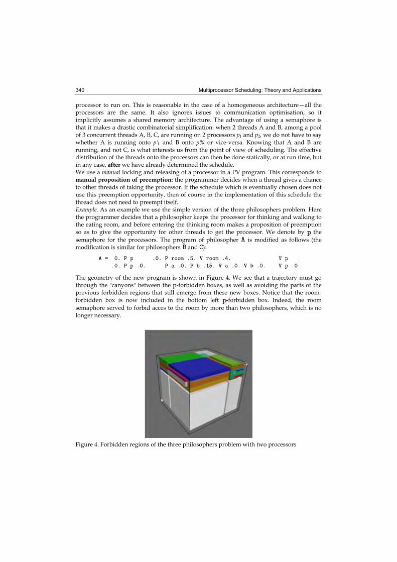
Multiprocessor Scheduling: Theory and Applications 340
processor to run on. This is reasonable in the case of a homogeneous architecture—all the processors are the same. It also ignores issues to communication optimisation, so it implicitly assumes a shared memory architecture. The advantage of using a semaphore is that it makes a drastic combinatorial simplification: when 2 threads A and B, among a pool of 3 concurrent threads A, B, C, are running on 2 processors p1 and p2, we do not have to say whether A is running onto p\ and B onto p% or vice-versa. Knowing that A and B are running, and not C, is what interests us from the point of view of scheduling. The effective distribution of the threads onto the processors can then be done statically, or at run time, but in any case, after we have already determined the schedule. We use a manual locking and releasing of a processor in a PV program. This corresponds to manual proposition of preemption: the programmer decides when a thread gives a chance to other threads of taking the processor. If the schedule which is eventually chosen does not use this preemption opportunity, then of course in the implementation of this schedule the thread does not need to preempt itself. Example. As an example we use the simple version of the three philosophers problem. Here the programmer decides that a philosopher keeps the processor for thinking and walking to the eating room, and before entering the thinking room makes a proposition of preemption so as to give the opportunity for other threads to get the processor. We denote by the
semaphore for the processors. The program of philosopher is modified as follows (the modification is similar for philosophers and ):
The geometry of the new program is shown in Figure 4. We see that a trajectory must go through the "canyons" between the p-forbidden boxes, as well as avoiding the parts of the previous forbidden regions that still emerge from these new boxes. Notice that the room-forbidden box is now included in the bottom left -forbidden box. Indeed, the room
semaphore served to forbid acces to the room by more than two philosophers, which is no longer necessary.
Figure 4. Forbidden regions of the three philosophers problem with two processors

A geometric approach to scheduling of concurrent real-time processes sharing resources 341
Limitations of the Approach. Remark that since each philosopher accesses 2 times a processor (through a lock of semaphore ), we indeed get 23 = 8 boxes that form the corresponding
forbidden regions. Computationally, it means that a thread should not propose preemption too often. On the other hand, finding the optimal schedule "for all possible preemptions" would imply, on the contrary, proposing a preemption between each event of the original program (which can be done automatically). But this would induce an exponential number of forbidden regions ( -forbidden regions).
On the other hand, this geometric approach can give new ideas for optimizations of the control of programs that run on a limited number of processors. For example, in the previous example, the geometry indicates that, in the given preemption is implemented, then the implementation can dispense with the semaphore.
7. Related Works
Timed PV Diagrams. Some other versions of timed PV diagrams have been proposed. We have not used them, for the reasons we explain below.
• The work [10], which presents a timed version of PV programs and diagrams, attempts to model multiple clocks, as in timed automata [4]. In the present paper we do not use the timed automaton model. Moreover, in the approach of [10] time is modeled as an additional dimension—one per clock. Thus, with one clock and three threads, a 4-dimensional space is studied. In this paper we consider each thread (or process) dimension as a "local time dimension", and then define the synchronization of local time dimensions.
• The work [14] exploits the dimension of each process as a time dimension. In this aspect, this work is close to ours. However there are important differences. First, the definitions in [14] are given in a continuous setting, and therefore topological spaces are considered, such that the duration of a schedule is described with an integral. In our work we stay in a discrete domain, an the definition of the duration of a schedule is given by an algorithm on a discrete structure. On the other hand, the fact that the definitions in [14] are tied to geometry implies, in particular, that zero-delays between two consecutive actions in a process (for example two successive locks, which often happens in programs that share resources) are not possible since the two actions would be the same in the geometry. In our approach, while we exploit the geometry to construct abstractions, the notion of duration itself is not geometric. Consequently, zero-delays are possible. This is of particular interest if one considers that the practical delay, on most architectures, between two consecutive locks, is too small to be modelled as a non-zero value. We conjecture that our version of timed PV diagrams is a discretized version of the continuous version of [14] (in the case of no zero-delays in the program).
Timed Automata. A large class of real-time systems can be adequately modelled with timed automata [4], and in this framework the problem of scheduling has been addressed [3,1, 2,16,17], often closely related to the context of controller synthesis. A timed PV program has a direct representation using timed automata. First, each thread is modelled as an automaton, where each node represents an event, and each transition from node e to node e' is labeled with constraint "i > d(e'y plus a reset of the clock. The global automaton is the product of all the thread-automata. Semaphores can be represented via variables. Such a

Multiprocessor Scheduling: Theory and Applications 342
product of automata is very close to that of [16], where the aim is also to schedule multi-threaded programs. In this work a scheduler is constructed to guarantee that a schedule does not go into deadlock states or deadline-breaking directions. We look for a complete schedule which is not only safe but also efficient; however our model is not as rich as the timed automata model: we have not yet included deadlines, branching, and looping. Scheduling and the Polytope Model. Another geometry-based method for scheduling concurrent programs is the polytope model (see, e.g., [8]), which is used in the context of automatic par-allelization. However the semantics of the points in the geometric space is not the same as in PV diagrams: each point inside a polytope represents a task which has to be executed, while in PV diagram each point is a possible state and only a very small number of these states have to be represented in the implementation. Also the polytope model does not consider resource sharing, and has no task durations.
8. Conclusion and Future Work
In this paper, we denned a timed version of PV programs and diagrams which can be used to model a large class of multithreaded programs sharing resources. We also introduced the notion of the worst-case response time of a schedule of such programs. This framework was then used to find efficient schedules for multithreaded programs. In particular, to tackle the complexity problem, we define an abstraction of the quickest schedules and we show how to exploit the geometry of PV diagrams to construct this abstraction and compute efficient schedules as well as a quickest one. This work demonstrates an interesting interplay between geometric approaches and real-time programming. An experimental implementation allowed us to validate the method and provided encouraging results. Our future work will explore the following directions.
• When developing a real-time system one is often interested in the worst-case response time of the whole program, if it is part of a larger system, for any schedule. As a definition, this WCRT could be given as the duration of the eager schedule that has the longest duration. We conjecture that we could use abstraction graph G for computing the longest eager schedule by computing the longest path in a subgraph of G. Defining this subgraph is a topic of our future research.
• We are able to find schedules, but it remains to see how they can be implemented. An obvious solution is controlling the computed schedule so as to enforce exactly the order of events it describes. But an interesting question is: among those control points, which can we "forget" while guaranteeing that the real execution will not diverge from the planned schedule as far as critical exchanges of resources are concerned? Indeed, in practice tasks can take less time than the WCET: control is needed for ensuring that such behaviour does not make the trajectory follow a direction which does not correspond to the schedule.
• We are currently investigating the problem of adding deadlines in our model. This extension is not straightforward since the "symmetry" with the definition of a lower bound to the duration spent by a thread between two consecutive events (the WCET of the task) is not trivial. We also intend to examine the possibility of lifting to the timed case the existing studies on the geometry of loops [12] or branching (if-then-else constructs) in PV programs.

A geometric approach to scheduling of concurrent real-time processes sharing resources 343
• Another approach to treat deadlines is to integrate our geometric abstractions into existing tools that use timed automata, such as [16]. These tools suffer from the problem of state explosion. Since our model is close to a product of automata, integrating our geometric approach into these tools could allow to handle larger systems.
9. References
Y. Abdeddaïm and O. Maler. Job-shop scheduling using timed automata. In Proceedings of the 13th International Conference on Computer Aided Verification (CAV 2001), LNCS 2102, pages 478-492. Springer Verlag, 2001.
K. Altisen, G. Gö iler, and J. Sifakis. Scheduler modelling based on the controller synthesis paradigm. Journal of Real-Time Systems, (23):55-84, 2002. Special issue on control-theoretical approaches to real-time computing.
R. Alur, S. La Torre, and G. Pappas. Optimal paths in weighted timed automata. In Proceedings of Fourth International Workshop on Hybrid Systems: Computation and Control, LNCS 2034, pages 49-62, 2001.
Rajeev Alur and David L. Dill. A theory of timed automata. Theoretical Computer Science, 126(2):183-235, 1994.
Olivier Bournez, Oded Maler, and Amir Pnueli. Orthogonal polyhedra: Representation and computation. In Proceedings of Hybrid Systems: Computation and Control (HSCC'99), LNCS 1569, pages 46-60. Springer Verlag, March 1999.
Manuel Clavel, Francisco Durán, Steven Eker, Patrick Lincoln, Narciso Martí-Oliet, José Meseguer, and Carolyn Talcott. Maude 2.0 Manual — Version 1.0. SRI International, June 2003.
R.egis Cridlig and Eric Goubault. Semantics and analysis of Linda-based languages. In Proceedings of WSA'93, LNCS 724. Springer Verlag, 1993.
Alain Darte, Yves Robert, and Frederic Vivien. Scheduling and Automatic Parallelization. Birkhauser, Boston, 2000.
E. W. Dijkstra. Co-operating sequential processes. In F. Genuys, editor, Programming Languages, pages 43-110. Academic Press, New York, 1968.
Ulrich Fahrenberg. The geometry of timed PV programs. In Patrick Cousot, Lisbeth Fajstrup, Eric Goubault, Maurice Herlihy, Martin R.aussen, and Vladimiro Sassone, editors, Electronic Notes in Theoretical Computer Science, volume 81. Elsevier, 2003.
Lisbeth Fajstrup, Eric Goubault, and Martin Rausen. Detecting deadlocks in concurrent systems. In International Conference on Concurrency Theory, pages 332-347, 1998.
Lisbeth Fajstrup and Stefan Sokolowski. Infinitely running concurrent processes with loops from a geometric viewpoint. In Patrick Cousot, Eric Goubault, Jeremy Gunawardena, Maurice Herlihy, Martin Raussen, and Vladimiro Sassone, editors, Electronic Notes in Theoretical Computer Science, volume 39. Elsevier, 2001.
Éric Goubault. Schedulers as abstract interpretations of higher-dimensional automata. In Proceedings of PEPM'95 (La Jolla). ACM Press, June 1995.
Éric Goubault. Transitions take time. In Proceedings of ESOP'96, LNCS 1058, pages 173-187. Springer Verlag, 1996.
Éric Goubault. Geometry and concurrency: A user's guide. Mathematical Structures in Computer Science, 10(4), August 2000.

Multiprocessor Scheduling: Theory and Applications 344
Christos Kloukinas, Chaker Nakhli, and Sergio Yovine. A methodology and tool support for generating scheduled native code for real-time Java applications. In Rajeev Alur and Insup Lee, editors, Proceedings of the Third International Conference on Embedded Software (EMSOFT 2003), LNCS-2855, pages 274-289, October 2003.
J. I. Rasmussen, K. G. Larsen, and K. Subramani. R.esource-optimal scheduling using priced timed automata. In Proceedings of the tenth International Conference on Tools and Algorithms for the Construction and Analysis of Systems (TACAS 2004), pages 220-235, 2001.

20
Sequencing and scheduling in the sheet metal shop
B. Verlinden1, D. Cattrysse1, H. Crauwels2, J. Duflou1 and D. Van Oudheusden1
1K.U.Leuven, Centre for Industrial Management 2Hogeschool voor Wetenschap en Kunst, De Nayer Instituut
Belgium
1. Introduction
1.1 History
Sheet metal operations have been in existence since 8000 B.C. (Fries-Knoblach, 1999). Due to its long history, sheet metalworking is, unfortunately, often seen as archaic and uninteresting. That metal sheets can be transformed with the aid of robust machines into fancy consumer products with tight tolerances is inconceivable to many. Yet, sheet metal operations are used for producing both structural components and durable consumer goods. Nowadays, sheet metal parts are widely present in different daily life products. During the past decades, scientific research in the field of sheet metal operations has been booming and international conferences on different sheet metal topics attract numerous attendants. Both industry and the academic community recognize the importance of continuing improvement in sheet metal operations. Thirty years ago, the rapid advance of computer systems triggered the introduction of automation in manufacturing environments. Also for sheet metal operations the use of computer systems has become indispensable to survive. Computer aided design (CAD) and computer aided manufacturing (CAM) systems are widely present in sheet metal production environments. At the earliest design stage, CAD systems are used to computerize the whole process of drawing and redrawing the desired part. Most modern CAD systems allow to build up a part from several re-usable 3D components, thus automating to a large extent the time consuming design process. The use of computers has also entered the manufacturing stage through computer aided manufacturing. The CAD file is converted into a sequence of processes for manufacture on a numerically controlled (NC) machine. The use of computers helps operators in automating different steps of the production process. As far as planning is concerned, most attention is focused on the computerization of sheet metal process planning. Production planning proper received much less attention due to a long tradition of experience-based production planning.
1.2 Scope of the research
If one queries the internet for sheet metal operations, numerous entries on processes are found, for instance on laser cutting, punching, deep drawing, bending, incremental forming,

Multiprocessor Scheduling: Theory and Applications 346
etc. Since many different sheet metal production processes and production environments can be identified, it is important to clearly delineate the scope of the research. The research as described in this chapter focuses on sheet metal operations in a flow shop environment (Figure 1). As far as the production processes are concerned, only laser cutting and air bending are considered.
Figure 1. Sheet metal operations
Figure 2. Typical sheet metal parts (a) complex part; (b) standard profile
Figure 3. The air bending principle
All parts follow a unidirectional flow in the sheet metal shop. In a preliminary stage, a large standard metal sheet or coil is cut to the right dimensions by using a pair of automated scissors (the shearing operation). Next, in the cutting stage, the unfolded blank of a part is punched with a punch press or cut with a laser machine. After cutting, the parts are bent

Sequencing and scheduling in the sheet metal shop 347
and transformed into 3D products. Air bending is used for this purpose. The air bending machine or press brake consists of a fixed bed on which the dies are fastened and a vertically movable ram (driven by hydraulic cylinders) on which the punches are mounted. A vertical force causes the ram to move down, forcing the sheet into the die, creating the bend line. The larger the vertical force, the smaller the bend angle (Figure 3). To produce a bend line of a part, a punch and die are required (called a tool set). The geometrical properties of the bend line (i.e. internal radius, bend allowance, type of profile, etc.) determine the characteristics of the required tool set. Punches and dies are supplied in sections (segments) for easy handling and quick set-up. If a long tool is needed, different segments are required. A combination of different segments to produce a single bend line is called a station. If a part consists of multiple bend lines, multiple stations are usually required (e.g. one station per bend line). Some stations may be used to produce several bend lines, while other stations can only be used for very specific lines. If a part requires different stations, all stations are positioned on the press brake with the required space between them, resulting in a production layout (Figure 4). A production layout can be used for bending several parts (depending on the geometrical properties of the part). This chapter mainly focuses on combinatorial optimization models and algorithms of use to production planning in Belgian small to medium-sized enterprises. Typically, in a Belgian SME, a single laser machine and press brake are available for production. Batch sizes range from a single workpiece to larger series (200 parts).
Figure 4. Press brake with a production layout consisting of three stations (every station is built up with different segments)
1.3 Outline
The research as described in this chapter evolved from a project in cooperation with a large sheet metal machine constructor and has been carried out by members of the Centre for Industrial Management, K.U.Leuven. The main goal of the project was to tackle a series of practical problems in a typical sheet metal shop. The chapter has six sections. Section 2 discusses some process planning issues for sheet metal laser cutting and air bending. An overview is given and relevant literature is mentioned. Section 3 elaborates on the tooling layout problem for air bending. The problem

Multiprocessor Scheduling: Theory and Applications 348
is analyzed and several solution procedures are proposed. Section 4 analyzes the production planning problem for air bending. A traveling purchaser problem approach (TPP) and a generalized traveling salesperson problem approach (GTSP) are proposed to reformulate the air bending production planning problem. Section 5 discusses production planning integration of laser cutting with air bending. The problems are highlighted and mathematical models are proposed. Computational results are discussed for a number of test cases. Section 6 concludes the chapter and formulates future research topics. In the chapter, mathematical models are formulated for the different planning issues, taking into account numerous problem-specific constraints. Typically, in a first stage, optimization procedures are used to obtain overall optimal solutions, but the computational effort required to solve combinatorial problems to optimality appears to grow very fast with the size of the problem. Local search, a class of heuristic methods, is applied at that point. It allows in a straightforward way to determine good, but not necessarily optimal solutions after a limited computational effort. In the problems discussed in this chapter two classes of local search techniques are implemented: simple neighborhood search and guided local search. Neighborhood search starts with a known feasible solution and tries to improve this solution by making well-defined moves in the solution space, shifting from one neighbor to another. A move is evaluated by comparing the objective function value of the current solution to that of its neighbor. In a pure descent method, only improving moves are allowed. When no further improvement can be found, the procedure ends. All feasible moves need to be defined and the search has to be initialized with a first solution. Although good choices for the different implementation issues can improve the performance of a descent algorithm, the resulting solution is, most likely, a local optimum, not a global optimum. A classical remedy for this drawback is to perform multiple runs of the procedure starting from different initial solutions and to take the best result as final solution (multi-start descent). Another possibility is to use a combination of different neighborhood structures (variable neighborhood search), as introduced by Mladenovi & Hansen (1997). In this way, a local optimum relative to a number of neighborhoods is determined. A more specialized type of local search is guided local search (GLS). The main feature of this approach is the iterative use of local search sequences. GLS penalizes, based on a utility function, unwanted solution features at the end of a local search sequence. In this way the solution procedure may escape from a local optimum and continue the search. The interested reader is referred to Voudouris & Tsang (1999).
2. Process planning issues
Besides production planning, the authors have used combinatorial optimization techniques also for a number of sheet metal process planning aspects. Next section discusses the state of the art regarding process planning issues and summarizes some of the process planning research conducted by the authors.
2.1 Process planning for laser cutting
Past decades steel prices have been increasing, resulting in a higher material cost for sheet metal parts. Hence, the amount of waste material needs to be minimized. In order to reduce the waste material, sheet metal parts with identical characteristics (material and thickness) are, if possible, combined on a large standard sheet to obtain high sheet utilization ratios.

Sequencing and scheduling in the sheet metal shop 349
The problem of combining different patterns on a flat blank or coil (apart from metal, the material can be paper, cardboard, leather, wood, plastic, textile, etc.) is known as the cutting stock problem and has received much attention. Alternatively, the name nesting is used. Numerous publications and applications can be found on this topic and a wide variety of solution techniques is proposed. Research on the cutting stock problem started with Eisemann (1957) discussing the problem of minimizing losses when cutting rolls of paper, textile, metal and other materials. This trim problem aims at allocating raws to machines and setting up the different cuts in such a way that the demanded rolls are cut to the right width, minimizing the overall trimming loss. Small problems are solved by enumerating the different possibilities. Most cutting stock problems were at that time formulated as integer programming problems to be solved with standard solution procedures. An overview is given by Haessler & Sweeney (1991). Research also focused on the determination of optimal sheet layouts. For such problems one has a number of rectangular sheets that need to be filled with two-dimensional regular and irregular shapes, minimizing the waste material. In the earliest days, researchers proposed to work with encaging rectangles. Adamowicz and Albano (1976) propose a two-stage approach. In a first stage, optimal rectangular modules are produced encaging one or more parts. In the second stage those modules are positioned on a sheet, minimizing the waste material. Working with encaging rectangles can only produce a rough plan since the exact shape of the parts is not considered. When personal computers with larger computational power became available, research shifted towards the nesting of the complex parts themselves instead of encaging rectangles. Lee & Woo (1988) developed a method to seek the minimal area convex hull of two convex polygons P and Q with Q being allowed to be translated along the boundary of P. If both translation and rotation operations are allowed, the problem of finding the minimal area convex hull becomes more difficult. The interested reader is referred to Nye (2001). Nesting remains an important issue in sheet metal cutting. Different peculiarities inherent to sheet metal production have to be taken into account when nesting different unfolded blanks on a large standard sheet. Prasad (1994) proposes some heuristic algorithms for nesting irregular sheet metal parts, taking into account grain orientation, minimum bridge width (i.e. the distance between two parts should be strong enough to withhold the bending force) and maximal material utilization. Tang and Rajesham (1994) propose an algorithm taking into account the rolling direction of the part. The rolling direction influences the brittleness of the part in both traverse and rolling direction. When bending the part this can cause the bend to crack at the bending edge. Generally it is assumed that a bend made at 30° to the grain flow is enough to avoid breakage. To overcome this problem, rolling direction information is taken into account at the nesting procedure. The method proposed approximates the part by a polygon with a sufficient number of sides to represent closely the original geometric shape. A more recent overview of sheet metal nesting is given by Valvo and Licari (2007). Besides the nesting proper, other related process planning issues received attention as well. After optimal nestings are generated, the cutting technology (laser power, cutting speed, position of the focal point, cutting gas pressure, stand-off distance between nozzle and material, lead-in, piercing method, etc.) and the cutting path need to be determined (taking into account common cuts, cutting distance minimization, heat build up in the material when cutting, etc.). Fortunately for the end-user, those different issues have been

Multiprocessor Scheduling: Theory and Applications 350
satisfactorily studied and are implemented in commercial nesting software. Such dedicated software tools allow the user to generate good nestings and to determine the cutting technology automatically.
2.2 Process planning for air bending
As for the laser cutting process, research on the bending process focuses on process planning. When a (3D) sheet metal part is produced with air bending, one starts from the unfolded blank of the required part (Figure 5). Gradually, this 2D flat blank is transformed into a 3D final workpiece by producing the different required bend lines. Different sequences are possible for producing the bend lines. Some bend sequences will cause collisions between the part, the machine and the tools while other sequences create no problems. The main goal of process planning is to determine an executable bend sequence and to select the different tools to use for each bend line, the gauging positions and the punch displacements.
Figure 5. Different unfoldings of a part
In order to determine the bend sequence, the different interactions between the part, the machine and the operator need to be investigated. For this purpose, a model is required representing the part during each of the consecutive process steps. If all geometric specifications, topological information, material characteristics and process related information would be included in such a representation model, the memory requirements could become very large. Some information, however, is redundant and only key information needs to be included. Duflou (1999) proposes a reduced foil model that contains only specific geometric information. This model also contains information regarding the topological relationships between the flange and the bend features of a part. For this purpose the part is represented by a graph with n nodes. The nodes represent the flanges, while the arcs represent the connecting features. The part can then be represented by a binary matrix, indicating whether two flanges are connected or not (Figure 6). For most parts the graph representation has to correspond with a spanning tree in the complete nxn graph. If loops are present in the graph representation scheme, a number of possibilities occur:
• the part can still be produced with air bending, but dedicated tooling will be required;

Sequencing and scheduling in the sheet metal shop 351
• the part can still be produced if a set of bends is simultaneously executed (so-called compulsory combined bends);
• no producible part’s unfolding can be determined: one or more bend connections need to be converted in weld connections or open seams.
The interested reader is referred to Duflou (1999). Additionally to the geometric and topological constraints, also technological constraints are enforced on the part. Non-compliance with those constraints causes the part to be infeasible to manufacture.
Figure 6. Part representation schemes (Duflou, 1999): (a) the 3D sheet metal part; (b) the unfolded blank of the part and the spanning tree; (c) the incidence matrix
Figure 7. Possible collision with (a) the punch and (b) the ram, when the bend sequence is not optimal
Thus the part representation scheme is used to determine the bend sequence and the gauging positions. The number of bend lines of the part, the number of gauging positions of the press

Multiprocessor Scheduling: Theory and Applications 352
brake and the different possible tools to produce the part tremendously increase the number of possible bend sequences. Duflou (1999) proposes a traveling salesperson problem based method to identify feasible (near-optimal) bend sequences. To limit in this TSP approach the number of possible candidate solutions, a number of criteria is used. Amongst others, ergonomic factors and productivity criteria are taken into account when verifying the feasibility of the different bend sequences. Also hard reject criteria (unavailability of proper gauging edges, collisions, non-compliance of the part dimensions with the specified tolerances, etc.) and soft criteria (e.g. looking at the ease of workpiece handling and total resource utilization) are used to reduce the number of candidate solutions. Each criterion is assigned a weight to be included in the TSP objective function. As such, a feasible (near optimal) bend sequence is determined from the remaining candidates. Bend sequencing is often integrated with tool selection (Nguyen, 2005). For each bend line a short list of possible tools is made based on technological and geometrical constraints. The technological constraints verify if the part can technically be made with the specific tool. Geometrical constraints check if there are any foreseeable collisions (Figure 7). In general a two-phase approach is followed. In the first phase (preselection phase) all nonconforming toolsets are eliminated for each bend line, based on the technological and geometric constraints. In the second phase (refined selection phase) the preselected tools are adjusted whenever a collision occurs to suit the stricter conditions imposed by this collision. Based on this data, the bend sequence is determined. The search procedure starts at the root node of the decision tree (the first bend line to be produced). Gradually, other bend lines are added to the intermediate bend sequence. At each node of the decision tree, collision detection tests are executed. If a collision occurs, all nodes from the same level are tested to detect a collision-free path. If no collision-free path can be determined, a tool change is executed if possible (Figure 8). To select a new tool (from the short list for that bend line), a number of rules are followed:
• minimize the number of tool profiles to be used for producing the part;
• maximize common preference for tools in a company;
• minimize the chance for sub-collision due to selection of a certain tool. A penalty system ensures that no redundant changes are made. The final result of the approach generates a collision-free bend sequence together with the different tools to be used for each bend stroke. The interested reader is referred to Nguyen (2005). For a comprehensive overview of other process planning issues, see Duflou et al. (2005).
Figure 8. Selecting the appropriate bending tooling to avoid collisions (Nguyen, 2005)

Sequencing and scheduling in the sheet metal shop 353
After determining the bend sequence and the tools, the physical layout of those tools on the press brake needs to be generated. A shrewd choice of the position of the different stations minimizes the total distance traveled for the operator during the bending process. Next section elaborates on this topic.
3. Tooling layout on a press brake for sheet metal air bending
3.1 Problem formulation
This section discusses the practical planning problem of locating all the required stations for a specific workpiece on a press brake. Process constraints and objectives regarding efficiency are taken into account. The n stations are mounted on a single press brake, their configuration is called the production layout (Figure 4). A station i has a length wi and li
and ri are the free spaces required respectively on the left and on the right side of station i. This free space depends on the bending operations assigned to the station, the intermediate shapes and the changing dimensions of the sheet metal part throughout the bend sequence. With the bend sequence S, a row of m station numbers is linked, specifying the order of the stations on which the m bending operations have to be executed. The actual location of all stations required for a specific workpiece on a press brake is determined by minimizing the total distance an operator has to travel during the processing of a specific work order. The main objective is to construct a fast algorithm for solving this problem because in a typical industrial environment, only a few seconds of computational time can be made available. Since exhaustive enumeration requires too much computational time, a neighborhood search method is suggested. The stations have to be located on a single line: the stations will be placed along the z-axis of the press brake. Experience with a large number of sheet metal parts allows to conclude that n=10 might be a safe upper limit for the number of required stations. Looking at the stations along the line, from the left to the right, the sequence of station numbers is a permutation of the n stations. Once a permutation is determined, the z-coordinate zi of each station, indicating the position of the middle of the station on the z-axis, is easily calculated. For any two stations i and j where i is located to the left of j, the following constraints have to be satisfied:
/ 2 / 2j i i j jz z w w l≥ + + + (1)
/ 2 / 2i j j i iz z w w r≤ − − − (2)
The quality of a specific layout can be calculated by the total distance traveled by an operator when he is executing a bend sequence:
1
1
1
| |i i
m
S Si
z z+
−
=
− (3)
where Si and Si+1 indicate the station numbers of two consecutive bending operations. Because this total distance traveled should be as small as possible, the stations will be placed as close as possible to each other, leaving no unnecessary space.

Multiprocessor Scheduling: Theory and Applications 354
Figure 9. Example of a station layout on a press brake
Figure 9 shows an example with n=2 stations. The parameters for station 1 and 2 are w1=100, l1=90, r1=70 and w2=80, l2=80, r2=50, respectively. In this layout, station 2 is placed at the first position and station 1 at the second position. From these relative positions, the absolute positions zi can be calculated:
2 2 2 / 2z l w= +
1 2 2 2 2 1/ 2 max( , ) / 2z z w r l w= + + +
For a bend sequence S=[1,2,1], the total distance traveled is equal to |300-120| + |120-300| or 360. Note that when the two stations exchange positions, the zi coordinates have to be recalculated (z1=140, z2=310). This is because the free space needed on the left of a station can be different from the free space required on the right side. Hence, the total distance traveled is not necessarily equal to the one of the first layout (|140-310| + |310-140| or 340).
3.2 Solution approaches
In the traditional approach no computer is used for determining the relative positions of the different stations on a press brake, only machine deformation considerations are taken into account. For the sake of symmetry and because both the table and the ram of a press brake are deformed during bending operations, the station for the longest bend line is located as centrally as possible. The second and third largest station are placed next to this largest station, one to the left and the other to the right, and this process is continued until all stations are placed. As a result, when going along the line of the stations from the left to the right, the stations become longer and longer until the longest station is reached; then they become smaller again until the end of the line is reached. This placing technique results in 2|n/2| possible solutions, because for each next pair of largest stations two alternatives exist: one station to the left of the partial layout and the other to the right and vice versa. The number of stations on a press brake is limited to 10, thus the maximum number of different solutions is equal to 25 = 32. This is a very small number and all the solutions can easily be generated by a computer by exhaustive enumeration. This approach is called the technical approach (EnumT). In a second approach, the length of the stations is not taken into account for determining the sequence of the stations. All possible solutions are listed by generating the n permutations of the set {1, 2, …, n}. For this optimal approach (EnumP) the minimal change order algorithm is used (Kreher & Stinson, 1999). In the third approach, the deformation of both the table and the ram of the press brake is again taken into account. This deformation is primarily caused by the largest stations and consequently, they should be placed as centrally as possible. The other, shorter stations can be placed freely along the line aside these few large stations. Parameter nw indicates the number of largest stations that have to be fixed in the middle of the line. For practical use,

Sequencing and scheduling in the sheet metal shop 355
the number of largest stations that should be placed as centrally as possible, can be calculated taking into account the geometrical aspects of the workpiece and the derived required forces during the bending operations. The solution procedure for this hybrid approach (EnumC) is a combination of the two procedures of the first two approaches. Permutations ( ) for the nw largest stations are generated by a procedure similar to EnumT and these stations are placed as centrally as possible. For each generated permutation, a procedure similar to EnumP is used to generate all permutations ( ) for the (n-nw) shorter stations. The first part of a permutation is placed to the left of and the rest to the right. In total, 2 nw/2 (n-nw)! alternative layouts have to be generated, except when n is even and nw is odd. In that case, the number of alternatives is twice this value. The computational effort required to solve the problems related to the optimal and the hybrid approach grows very fast with the size of the problem. Therefore, descent methods are developed to solve these problems. For the optimal approach, the natural representation is a permutation of the integers (1, …, n) with n the number of stations. On this representation, two basic neighborhoods can be defined. With insert (INS) a station is removed from one position in the sequence and inserted at another position (either before or after the original position). General pairwise interchange (GPI) or “swap” swaps two stations. A special case is API adjacent pairwise interchange where the two stations are adjacent. For the order in which the neighborhood is searched, a fixed natural lexicographic ordering is used, i.e. (1,2), (1,3), …, (1,n), (2,1),(2,3),…, (i,j), …, (n-1,n), with i and j the two station numbers (for GPI only pairs where i<j are considered). Each time an improving move is executed, the next iteration restarts at the beginning of the ordering. Different initial solutions were investigated. With at random, the first solution is equal to the permutation of the different stations in numerical order, i.e. (1,2, …, n). In the most visited initial solution, the station that is visited most frequently is placed in the middle of the line. The others are placed to the left and to the right of this station in order of descending frequency of use. The start bend sequence seed is created in accordance to the sequence of bending operations. This can be a promising initial solution when most stations are visited only once. The end bend sequence seed is analogous to the previous method, but the search is started at the end of the bend sequence and continues in reverse order through the sequence. For each of these four initial solutions, an additional initial seed is considered by using the generated solution in reverse order. By performing multiple runs of the procedure starting from the eight different initial seeds and taking the best sequence as final solution, we get a multi-start descent solution approach. For the hybrid approach, only a descent method for the placement of the shorter stations is considered. In practical situations, the number of largest stations nw is small and all corresponding permutations can easily be generated by exhaustive enumeration. The neighborhood is a variation of the swap neighborhood defined for the optimal approach: only stations from the first part (before the fixed largest stations) and from the last part (after the fixed largest stations) are considered for a pairwise interchange. The initial seed is a layout that satisfies the specifications of the technical approach. The fixed largest stations are already positioned as centrally as possible. Around this fixed part, the other stations are added in an order from long to short.

Multiprocessor Scheduling: Theory and Applications 356
3.3 Computational experience
For the computational tests, the enumeration algorithms and the descent techniques were coded in C and run on a HP 9000/L1000 computer. The data set (with 48 instances) used to test the different procedures is at random data offering a good approximation for real instances. An optimal solution value to each problem is obtained with the enumeration algorithm EnumP. For problems with up to n=8 stations, this exhaustive enumeration requires less than one second of computational time. The longest computational time is used for problems with n=10 stations, i.e. nineteen seconds. The performance of the technical approach and the hybrid approach and of the heuristics for the optimal approach is compared by listing the number of times (out of 48) that an optimal solution is found (NO), the average relative percentage deviation (ARD) of the solution value from the optimal value and the maximum relative percentage deviation (MRD) from the optimal value. Table 1 compares the results when using the technical approach or the hybrid approach (with nw the number of fixed largest stations) instead of the more ideal station layout based on the optimal approach. It is clear that a lot more distance has to be traversed when a layout based on the first approach is used. Note that the ARD and MRD performance measures are not an indication for the bad performance of the solution procedures. They just give information about how much the layouts based on the technical or hybrid approach deviate from the optimal layout because of the additional process constraints. For some instances, this distance is more than twice the distance resulting from a layout based on the optimal approach. The results of Table 1 indicate that it is worthwhile to consider the hybrid approach, where only a few large stations are fixed as centrally as possible. In most practical situations, fixing the largest station in the middle is adequate to prevent an asymmetrical deformation within one bend line. The column with label nw=1, shows that the total distance traveled is on average raised with 10%.
EnumT
nw=1 nw=2 nw=3
NO 6 14 6 6
ARD(%) 54.84 10.43 24.36 37.60
MRD(%) 259.67 46.60 66.30 135.60
EnumC
Table 1. Results of the enumeration algorithms
When more large stations have to be fixed in the middle of the line, the additional distance that has to be traversed, increases. Hence, it is important that stations that cannot cause any significant deformation, are freely placed on the line in order to minimize the total distance traveled as much as possible. The left part of Table 2 shows the performance of the multi-start descent method on the optimal approach considering the three neighborhoods, adjacent pairwise interchange (API), general pairwise interchange (GPI) and insert (INS). This method requires less than one second for each instance of the data set.

Sequencing and scheduling in the sheet metal shop 357
API GPI INS nw=1 nw=2 nw=3
NO 29 39 47 29 35 42
ARD(%) 1.84 0.33 0.02 1.66 1.07 0.22
MRD(%) 13.71 5.01 0.85 13.51 14.44 4.63
Hybrid approachOptimal approach
Table 2. Neighborhood search results
Note that in this table the ARD and MRD performance measures are an indication for the effectiveness of the heuristic solution procedure. One of the characteristics of a neighborhood for determining the effectiveness is its size, i.e. the number of neighbors for a single solution. The sizes of the used neighborhoods are (n-1) for API, n(n-1)/2 for GPI and (n-1)2 for INS. With a larger neighborhood, more diversity can be introduced in the search and this generally results in a better performance as can be observed in the left part of Table 2. The number of problems solved to optimality increases and the average relative deviation decreases when a larger neighborhood is used. It is worthwhile to investigate the performance of the neighborhood search technique for solving problems based on the hybrid approach. For instances with n=10 stations, exhaustive enumeration requires about four seconds of computational time. In the right part of Table 2, the results of the descent method based on a swap neighborhood are compared with the values calculated with the enumeration procedure for the third approach. Quite good results are obtained: a lot of instances are solved to optimality and the average relative percentage deviation is small. The fact that only a single-start version is used, is probably the cause for the large MRD value. It is remarkable that the performance of the heuristic increases when the number of fixed stations nw increases. With a larger nw value, the solution space is smaller and the swap neighborhood is probably capable to search this space adequately.
3.4 Summary
This section presents some practical methods for placing a number of stations consisting of a punch and a die, on a press brake for sheet metal air bending. Comparing the best values of the total distance traveled according to the technical approach and to the optimal approach, indicates that a lot of traveling distance can be saved when the tooling layout is based on the optimal approach. Yet, when very large stations have to be used for producing a workpiece, one cannot ignore the asymmetric machine deformation. Therefore, a third approach is suggested. In this approach only the largest stations are placed as centrally as possible and the other stations are freely added to the left and to the right of these largest stations. The computational results indicate that layouts based on this hybrid approach are to be preferred, especially when only one large station has to be fixed in the middle. Apparently, a simple neighborhood search technique gives good results. After the physical layout of the different stations on the press brake is determined, the part can be produced with air bending. Production planning for air bending is usually carried out by an experienced operator. Makespan reduction is the most important criterion in this process. Since interchanging production layouts is time consuming, such set-ups should be avoided as much as possible. Section 4 discusses the authors’ effort to automate production planning for press brakes and to improve on the schedules of an experienced production planner.

Multiprocessor Scheduling: Theory and Applications 358
4. Automated production planning of press brakes for sheet metal bending
4.1 Problem formulation
For bending, every part requires a specific production layout and the time to produce this part depends on the properties of the layout. Changing production layouts is time consuming and should be avoided. Fortunately, some production layouts can be used for several parts. For instance a bend line with length (k) can be made with a tool set length (k+x) if that bend line does not contribute to forming a box-type part. The other way around is impossible: a bend line with length (k) cannot be made with a tool set length (k-x). Table 3 presents a small example with four jobs and six production layouts. Job 1 can be processed using production layout a in 100 seconds, using production layout d in 130 seconds, or using production layout f in 120 seconds. With production layout d it is possible to produce jobs 1, 2 and 3. Table 4 summarizes the set-up times between the different production layouts; the matrix is inherently an asymmetric one. The different possible production layouts per job and the different possible production layouts for combinations of jobs can be generated by a computational procedure (see e.g. Duflou et al. 2003) starting from the complete (initial) set of jobs. The different manipulations during set-up from a particular layout to another one can be analyzed; standard time and motion studies will provide set-up time estimates. Furthermore, time and motion analysis allows for the calculation of production times (Vansteenwegen & Gheysens, 2002).
Job a b c d e f
1 100 - - 130 - 120
2 - 60 - 90 - 80
3 - 40 - 70 50 -
4 140 - 120 - 60 -
Production layout
Table 3: Feasible production layouts per job and corresponding production times (seconds)
Production layout end a b c d e f
start - 72 58 48 79 53 48
a 55 - 74 136 38 324 0
b 30 128 - 22 184 90 210
c 36 40 40 - 70 50 164
d 63 140 32 38 - 60 112
e 35 200 152 34 30 - 110
f 35 20 90 38 118 18 -
Table 4: Set-up times between the production layouts (seconds)
Currently, production planning practices for bending are based on experience. The press brake operator receives a work list with parts to bend. Based on his knowledge and skill, the production layouts are selected and the parts scheduled. Until now, no assisting software packages are available on the market. Typically, the task of a production planner should be:
• select for each job a production layout, minimizing the total production time;

Sequencing and scheduling in the sheet metal shop 359
• sequence the different jobs at the press brake, minimizing the makespan for the pool of jobs.
For the example (Table 3 and Table 4), a feasible solution is layout sequence [e - f] with jobs 1 and 2 assigned to production layout f, while jobs 3 and 4 are assigned to production layout e. The makespan for this small set of orders equals 53 + (50+60) + 110 + (120+80) + 35 = 508 seconds. Apparently, the Press Brake Planning problem (PBP) has a very specific structure. Two well known models from the literature, the traveling purchaser problem (TPP) and the generalized traveling salesperson problem (GTSP) can capture this structure. Both modeling approaches are investigated to verify whether production planning for air bending can be automated, minimizing the makespan, or not. The computational requirements and quality of the final solution are determinant factors when comparing the two methods. Next subsections discuss both lines of action.
4.2 The traveling purchaser problem (TPP)
Ramesh (1981) describes the TPP as a generalization of the traveling salesperson problem (TSP). An agent must visit a number of markets/cities in order to buy, at minimum cost, a set of items. The cost consists of two elements: the travel cost between the markets and the purchase cost of the items. The production planning problem for air bending is now reformulated, using following parameters and variables:
• i,j: indices for markets
• k: index for the product
• cij: travel cost when traveling from market i to market j
• hik: purchase cost for product k at market i
• xij: binary variable indicating whether or not the agent travels from market i to j
• yik: binary variable indicating whether product k is bought at market I
• I: all cities/markets, where 0 is the starting position of the agent (I0 = I \ {0})
• K: all products
| | | | | | | |
0 0 1 1
I J I K
ij ij ik iki j i k
Min c x h y= = = =
+ (4)
. . s t| |
1
1I
iki
y k K=
= ∀ ∈ (5)
| |
0
I
ik ijj
y x=
≤ , 0;i I k K∀ ∈ ∀ ∈ (6)
| | | |
0 0
I I
ij jij j
x x= =
= , i I∀ ∈ (7)

Multiprocessor Scheduling: Theory and Applications 360
| |
0
1
1I
ii
x=
= (8)
1iji S j S
x S∈ ∈
≤ − , 0S I⊆ (9)
{ }0,1ijx ∈ , ( , ) ,i j I k K∀ ∈ ∀ ∈ (10)
In formulation (4)-(10), the objective function (4) minimizes the total cost. Constraints (5) ensure that all products are purchased. Constraints (6) allow to buy a product only when a market is visited. Constraints (7) are the balancing constraints: a market entered has to be left as well. Constraint (8) indicates the tour starts at the starting point. Constraints (9) are the subtour elimination constraints and constraints (10) limit the variables to Boolean values. The example from Table 3 is represented as a TPP instance in Figure 10. The squares (cities) represent the production layouts, the circles (items) the jobs. The traveling costs between the cities are the set-up times between the production layouts, while the purchase costs are the production times of the parts, given a specific production layout. Some parts or jobs (circles) are connected by arrows to several production layouts (squares) since some jobs can be produced with a few production layouts. The dotted arrows represent a feasible job allocation: only two production layouts are chosen, e and f. Jobs 3 and 4 are produced with layout e; jobs 1 and 2 are produced with production layout f. In total, the production time equals 310 seconds and the total set-up time is 198 seconds. This results in a makespan of 508 seconds. Several procedures are available to solve the TPP. The interested reader is referred to Ramesh (1981), Pearn (1991) and Singh & Van Oudheusden (1997).
Starting position
c
e
b
1
3f
2
4
da
Job
Production layout
Figure 10. TPP presentation of the example

Sequencing and scheduling in the sheet metal shop 361
Heuristic solutions of the TPP can be generated in different ways, depending on the emphasis put on either production or set-up times. If one only wants to minimize the number of set-ups a set covering formulation can address the problem (E. El-Darzi & G. Mitra, 1995). Generally speaking this approach will yield poor results with regard to makespan since production and set-up times are not taken into account. For the example presented in Tables 3 and 4, many solutions with only two set-ups appear, i.e. -a-b-, -b-a-, -a-d-, -d-a-, -e-f-, -f-e-, -c-d-, and -d-c-. But the makespan varies quite a lot: respectively 516, 581, 573, 674, 508, 411, 591 and 563 seconds. A much better approach, fitting the intrinsic TPP structure, would be a hierarchical decomposition procedure. In a first step a simple plant location problem (SPLP) is solved for instance by means of the procedure of Erlenkotter (1978), using average set-up times between the production layouts as the fixed costs for the different plants. In this way each workpiece is assigned a production layout, minimizing the total number of layouts for the pool of workpieces. In a second step a TSP is solved to determine the sequence for bending the different parts. Real set-up costs between the production layouts are used as the traveling costs.
4.3 The generalized traveling salesperson problem (GTSP)
The GTSP (Srivastava et al., 1969) is the problem of finding a minimum length tour through a predefined number of subsets of customers while visiting at least one customer in each
subset. The node set N consists of m mutually exclusive node sets SI such that N = S1 ∪ S2 ∪…Sm and SI ∩ SJ = ∅ for all i and j (i ≠ j). Assume that arcs are defined only between nodes belonging to different sets. The objective is to find a minimum length tour visiting a node in every set. Following parameters and variables will be used in the formulation:
• i,j: indices for the cities
• cij: travel cost when traveling from city i to city j
• xij: binary variable indicating whether or not the salesperson travels from city i to j
• A: all arcs connecting two cities
• N: all nodes
( , )
ij iji j
Min c x∈Α
(11)
. . s t
( , )
. . 1I I
iji S j S
i j
s t x∈ ∉
∈Α
= , IS∀ (12)
( , )
1I I
iji S j S
i j
x∉ ∈
∈Α
= , lS∀ (13)
( , ) ( , )
0ij jki N k Ni j A i j A
x x∈ ∈∈ ∈
− = , j N∀ ∈ (14)

Multiprocessor Scheduling: Theory and Applications 362
( , )
1I J
ijI i S J j S
i j A
x∈ℑ ∈ ∉ℑ ∈
∈
≥ , sets , 2 2,m w∀ ℑ ≤ ℑ ≤ −
which are proper subsets of the collection of node sets (15)
{ }0,1ijx ∈ , ( , )i j A∀ ∈ (16)
The objective function (11) minimizes the total traveling cost. Constraints (12) and (13) ensure that in every subset one node is visited. Constraints (14) indicate that an entered node j has to be left as well. Constraints (15) are subtour elimination constraints, while constraints (16) limit the variables to Boolean values. A graphical representation of the GTSP formulation of the previous example with the same feasible solution is seen in Figure 11.
a
f
Job 1
b
f
Job 2
d
b
e
Job 3
a
e
Job 4
Starting position
dd
c
Figure 11. GTSP presentation of the example
The arrow cost comprises the set-up cost between the production layouts and the production cost of the jobs with a certain production layout. In this way the traveling costs represent set-up as well as production time. Exact algorithms are available to tackle the problem but since the procedure has to run on line, heuristic procedures are preferred. For GTSP, local search algorithms can be quite naturally developed (Johnson & McGeoch, 1997). A feasible solution can be represented by a permutation vector of size m, each element representing a customer belonging to one subset. The feasible solution of Figure 11 can be represented by { e4, e3, f1, f2 }. It is simple to create a neighborhood by using a 3-opt procedure, i.e. removing three arcs and rearranging the order of the three resulting parts. Once a new order is fixed, it is accepted and declared to be the new current solution if the makespan is reduced. To speed up the local search procedure not the complete neighborhood is investigated, but only changes leading to neighbors that look promising.

Sequencing and scheduling in the sheet metal shop 363
This descent procedure is then embedded in a guided local search procedure where long arcs , which are unlikely to appear in a good tour, are penalized. The lengths of some arcs of the current solution are thus artificially increased and the local search procedure is recalled, hoping to escape in this way from the local minimum death trap.
4.4 Computational results
Test problems are generated based on real-life data from different test companies. The test cases comprise 10, 15 or 20 orders. A distinction is made between complex parts and standard profiles (Figure 2). The production layout used for producing a standard profile can most likely be used for other profiles as well due to the simple structure of the profiles (mostly a single bend line). For producing a batch of orders comprising mainly (or exclusively) profiles, less production layouts are required compared to a batch of orders comprising complex parts. Indeed, the probability that a production layout (PL) of a complex part can be used for bending another complex part is rather small. In general one can observe that by decreasing the number of profiles from the pool of orders, on average, the number of required production layouts is increasing. The problems encoded with an index a (SMBXXa) refer to problems which contain 50% or more profiles and with an index b (SMBXXb) to problems with less than 50% profiles (see table 5). The algorithms for solving TPP and GTSP were coded in C/C++ and were run on a personal computer (Pentium 4, 2.66 GHz, 256 Mb RAM) under Windows XP. The results are based on single runs for each problem.
PBPs TPP GTSP REF
All 4.71 4.41 12.98
SMB10 4.25 3.99 12.19
SMB15 4.59 4.37 12.97
SMB20 5.59 5.12 14.19
SMB10a 4.42 4.42 10.03
SMB10b 4.11 3.63 14.09
SMB15a 4.40 4.19 11.12
SMB15b 4.72 4.48 14.25
SMB20a 4.52 4.49 11.27
SMB20b 6.05 5.39 15.44
Average deviation from lower bound (%)
Table 5. Computational results
For each problem, a lower bound (LB) and a "reference" solution (REF) are calculated. The lower bound is based on the simple plant location problem solution using the smallest set-up time as the fixed cost. The makespan value of the reference solution is calculated as follows: the best production layout is selected for every job and then the jobs are sequenced. One can interpret this makespan as the time a good production planner would obtain by solving the press brake planning problem by hand. Table 5 summarizes the deviation (%) from the lower bound. The average deviation is given for all problems, for each problem set

Multiprocessor Scheduling: Theory and Applications 364
and also for every problem split up according to a (50% profiles or more) and b (less than 50% profiles). Table 6 contains the calculation time to obtain these solution values. The TPP column gives the solution values obtained by the hierarchical approach, the GTSP column the solutions obtained with the guided local search procedure, the REF column is the reference solution value and the LB column gives the lower bound. The results indicate that it is worthwhile to apply the TPP or GTSP approach instead of relying on the results of an experienced production planner. The solution improves by 8 % on average. The improvement is larger for problems with fewer profiles, the deviation goes up to 10 % while for problems with a larger number of profiles it varies around 7 %. The difference originates from the fact that for the problems with a fewer number of profiles less process plans are generated by a human production planner than by the automatic production planner. Moreover, the more parts included in the pool of orders, the more difficult it becomes for an experienced production planner to keep a good overview of the planning process. A human production planner rarely combines different jobs to be produced with a single production layout because mentally he cannot take into account all possible combinations. The simple TPP hierarchical approach is amazingly good. The difference between the TPP approach and the GTSP approach is quite small, especially for the problems with many profiles. For profiles there are less set-ups required since a few layouts can be used for many products. But if less profiles appear in the work orders, set-ups become more important and the performance of the hierarchical approach gets worse as can be seen in Table 5. The difference in deviation between the TPP and GTSP approach is always smaller for the
SMBXXa problems (≥ 50% profiles). When set-up importance is increasing, the hierarchical procedure is not working as well.
PBPs TPP GTSP REF LB
All 0.06 83.26 0.00 0.01
SMB10 0.02 29.51 0.00 0.00
SMB15 0.04 65.59 0.00 0.03
SMB20 0.15 190.40 0.00 0.00
SMB10a 0.02 11.26 0.00 0.00
SMB10b 0.03 45.48 0.00 0.00
SMB15a 0.03 16.24 0.00 0.00
SMB15b 0.05 90.27 0.00 0.04
SMB20a 0.07 45.24 0.00 0.00
SMB20b 0.18 252.61 0.00 0.00
CPU time (seconds)
Table 6. CPU times
The TPP approach has the advantage that a solution is determined in a very small amount of time. It never takes more than 0.5 seconds to generate a solution. Solving the SPLP takes less than 0.01 seconds, the remaining time is for the local search approach (10,000 iterations), which solves all the TSP problems tested to optimality in less than 0.05 seconds on average. The solution time of the guided local search procedure solving the GTSP formulation is

Sequencing and scheduling in the sheet metal shop 365
linear in the number of iterations allowed. The reported computation times are limited to 100,000 and take on average 90 seconds.
4.5 Summary
The purpose of this research is to investigate the possibility of automating the complete production planning function and, if possible, improving on the schedules of an experienced production planner. In this section the press brake planning problem is discussed. Two approaches, the TPP and GTSP approach, are tested. The hierarchical decomposition approach (TPP) produces good results and requires only little time (less than 0.5 seconds for the larger problems) so that the procedure can be used on line to generate the production plan at the beginning of a day or when rush orders arrive during the day. The GTSP approach yields better results but requires more time. Additional tests indicate that the time estimates for set-up and production times are sufficiently accurate and robust; more importantly the makespan values generated by the TPP and GTPS approaches appear to be very realistic. The conclusion therefore is that the production planning of press brakes for sheet metal bending can indeed be automated. In this way, considerably more efficient planning can be achieved and less time has to be spent on the frequent planning and replanning of the different steps. The modeling and algorithmic intricacies of the approach appear to be modest. The success of the TPP and GTSP approaches is due to the optimization of trade-offs between set-up and production times. Generally speaking, this optimization will become better when more choices can be made; the number of choices being a function of the number of considered production layouts. Thus it is important to consider, from the outset, a sufficiently large set of possible production layouts. Detailed analysis could determine how precisely the solutions are affected by changes in the set of possible production layouts. The different algorithms for the press brake planning problem have not been implemented in commercial applications yet. Experience-based planning practices are still omnipresent at the bending stage. Although laser cutting and air bending planning can thus be optimized, simply sequencing the optimal solutions of the two processes can create problems for the sheet metal flow shop. Section 5 addresses these issues.
5. Integrated approach for production planning
5.1 Need recognition
As discussed, certain process planning issues and production planning issues can be optimized separately for laser cutting and bending. However, the optimization of the distinct processes gives no guarantee for a globally optimized situation. Optimization decisions taken at one production stage influence the preceding stages. As such, the different objectives can counteract one another creating a non-optimal situation for the complete production chain. This actually happens when looking at the sheet metal flow shop with laser cutting and air bending. At the cutting stage, nesting software is used to determine the sheet layout that generates the best material utilization for the available workpieces. Low scrap percentages are preferred and if parts of the sheet are unused, remnant sheets are stored for later use. After the workpieces are cut (sheet by sheet), they are sent to the press brake for bending (if a 3D workpiece is required). At the press brake, an experienced operator tries to reduce the set-ups between production layouts as much

Multiprocessor Scheduling: Theory and Applications 366
as possible. However, since at the cutting stage no information regarding the required bending tools was taken into account, multiple set-ups occur at the press brake. In the worst case scenario, every single workpiece of a sheet requires a different production layout for bending. If multiple set-ups are required, a substantial amount of time is needed to produce the workpieces. Distinct step optimization thus leads to counteracting benefits: the effort spent on nesting is counteracted by an increased number of set-ups at the press brake. Another trigger for an integrated production planning approach is the fact that currently production planning is mainly experience based. Although experienced operators are able to generate feasible production plans, there is ample space for improvements. The press brake operator will sequence the jobs that are physically waiting in front of the press brake. For a small amount of workpieces he will get a clear overview of the different possibilities. However, if many workpieces are available for bending, he may get lost in the process. In those cases he will generate a feasible but not optimal solution since an experienced operator will most likely not consider all possibilities. Another important remark should be made. The press brake operator will do his best to sequence the workpieces waiting in front of the press brake with as little set-ups as possible. Unfortunately, this operator has no overview of all workpieces that need to be produced in the coming period. It may thus happen that determining a good sequence for the current batch turns out to require multiple set-ups for the next period. An integrated approach should take all workpieces into account and generate a production sequence with a reduced makespan for the complete set of orders.Thus, computerizing the production planning process and approaching it from an integrated perspective offers several opportunities:
• one looks at the complete picture to generate a plan for the coming T time buckets;
• one verifies automatically more possibilities than an experienced operator;
• one integrates both production stages to avoid counteracting benefits. The research as described in this section aims at producing such integrated production plans.
5.2 Mathematical model for the integrated production planning problem
5.2.1 IP formulation
For solving the integrated production planning problem, an integer programming formulation (IP) is proposed. A number of variables and parameters are defined:
• i: workpiece index
• l: production layout index
• k: sheet index
• fl: average set-up time for production layout l
• zik: binary parameter indicating if workpiece i can be nested on sheet k
• pil: bending time for workpiece i with production layout l
• cil: binary parameter indicating if workpiece i can be bent with production layout l
• Ai: surface of workpiece i
• li: length of workpiece i
• wi: width of workpiece i
• Ck: capacity of sheet k

Sequencing and scheduling in the sheet metal shop 367
• lk: length of sheet k
• wk: width of sheet k
• xilk: binary variable indicating if workpiece i is assigned production layout l and nested on sheet k
• ylk: binary variable indicating if production layout l is used for sheet k
• I: all workpieces
• L: all production layouts
• K: all sheets The IP formulation for the problem becomes:
| | | | | | | | | |
1 1 1 1 1
minL K I L K
l lk lk ill k i l k
f y x p= = = = =
+ (17)
. . s t
ilk lkx y≤ , ; ;i I l L k K∀ ∈ ∀ ∈ ∀ ∈ (18)
| | | |
1 1
1L K
ilkl k
x= =
= , i I∀ ∈ (19)
ilk ilx c≤ , ; ;i I l L k K∀ ∈ ∀ ∈ ∀ ∈ (20)
ilk ikx z≤ , ; ;i I l L k K∀ ∈ ∀ ∈ ∀ ∈ (21)
| | | |
1 1
I L
ilk i ki l
x A Cα= =
≤ , k K∀ ∈ (22)
ilk i kx l l≤ , ; ;i I l L k K∀ ∈ ∀ ∈ ∀ ∈ (23)
ilk i kx w w≤ , ; ;i I l L k K∀ ∈ ∀ ∈ ∀ ∈ (24)
, {0,1}ilk lkx y ∈ , (25)
The objective function (17) of the IP model has two components. Firstly, the number of set-ups at the press brake is minimized. There is an average set-up time fl associated with every production layout l used per sheet. Every time a production layout is selected for a certain sheet, the objective value is increased with the average set-up time for that production layout. This formulation assures that as few as possible production layouts are selected for a sheet, thus minimizing the set-ups at the bending stage. If a new production layout is required, preferably one with a low average set-up time is chosen. As such, workpieces requiring the same production layout will preferably be combined on the same sheet,

Multiprocessor Scheduling: Theory and Applications 368
creating less set-ups at the press brake. Secondly, the total bending time at the press brake is minimized. A workpiece's bending time is influenced by the selected production layout for bending. The second part of the objective function assures that workpieces are assigned to a production layout with low bending times in order to decrease the makespan of the pool of jobs. Constraints (18) make sure that a workpiece can only be assigned to a specific production layout for a sheet, if that layout is selected for that particular sheet. The binary ylk variable will increase the objective function, every time a new production layout is required. Constraints (19) indicate that each workpiece should be produced, i.e. each workpiece should be assigned to a production layout and should be nested on a sheet for cutting. Constraints (20) limit the layouts that can be used for a certain workpiece. The binary workpiece-layout matrix indicates whether a certain workpiece i can be made with layout l. Not all workpieces can be produced with all available production layouts because of restrictions imposed by the workpiece’s geometry. Constraints (21) verify if a workpiece can be nested on a certain sheet, based on the material type and the sheet thickness. Constraints (22) guarantee that the total usable area (Ck) of a sheet is not exceeded while nesting the different workpieces. A safety zone ( ) is taken into account. This ( ) takes into account the required spacing between workpieces (heat build-up when cutting) and the clamping zone. Constraints (23) and (24) check the length and width of a workpiece compared to the length and width of a particular sheet to avoid creating infeasible nestings. Constraints (25) limit the decision variables to Boolean values. The result of the mathematical model (17-25) determines for each sheet which workpieces should be combined for cutting (nesting). It is important to note that the actual arrangement of those workpieces on the sheet is not generated by the IP model. Dedicated algorithms, implemented in commercial software, allow to generate the best arrangement, taking into account process planning aspects such as heat build up when cutting, piercing of initial holes, cutting path minimization etc. It is not the purpose of this research to introduce process planning issues in the production planning module. Besides the groupings of the workpieces, the IP model also indicates for each workpiece the required production layout for bending. The total number of production layouts is thus minimized and all workpieces are assigned to a unique production layout. Besides a possible makespan reduction (due to the reduced set-up time at the press brake), material utilization plays an important role. Minimization of the number of sheets is not as such included in the mathematical model. The number of sheets is fixed in advance (user-defined). This number can be determined based on:
• the theoretical number of sheets: for every material type and sheet thickness, the total parts' area is divided by a sheet's area and rounded upwards and the necessary margins for clamping, etc. are taken into account;
• the optimal number of sheets as determined by dedicated nesting software: commercial packages can be used to determine for each material type and thickness the amount of sheets required.
The exact production sequence for the different sheets is not determined by the IP model. Since the sheet metal shop is seen as a flow shop with single machines at each stage, the order of cutting the sheets also determines the order of bending the sheets and vice versa. In the presented research, the order of cutting the sheets is determined by the bending stage. This means that the sheets are sequenced such that the set-ups between production layouts of consecutive sheets at the press brake are minimized. It is important to notice that when

Sequencing and scheduling in the sheet metal shop 369
talking about the bend sequence, one usually discusses the sequence in which the bend lines of an individual workpiece need to be executed to avoid collisions. For production planning issues, the bend sequence indicates the sequence in which the different sheets need to be bent. To avoid this confusion, a specific terminology has been developed:
• Bend sequence: is shown on the process plan and gives the sequence for producing the different bend lines of a workpiece (to avoid collisions when bending the workpiece, e.g. bend line 1 - bend line 5 - bend line 3 - etc. ).
• Production sequence: is related to the production plan and gives the sequence for cutting and bending the sheets (e.g. sheet 1 - sheet 4 - sheet 3). The term production sequence is used for flow shops with a single machine at each stage (the production sequence for cutting is then the production sequence for bending).
• Production bend sequence: is mentioned on the production plan and indicates for a sheet the sequence in which the different workpieces of that sheet need to be bent (e.g. workpiece 1 - workpiece 12 - workpiece 3).
The IP model neither generates the production sequence nor the production bend sequence for the different sheets. Thus, some additional steps are required to generate the final production plan. The list from the IP model indicates for each sheet the different workpieces to bend and the production layout to use. A TSP instance is solved for each sheet with the sequence-dependent set-ups between the production layouts as travel distances. The result of this step is a list with the different sheets, and the production bend sequence for bending the workpieces of each sheet. Next, a TSP instance is solved to determine the production sequence for the different sheets. In this last step, the sheets can swap/shift positions, but the production bend sequence of a sheet cannot be altered anymore. Table 6 displays a typical final production plan.
Demostuk (PL181) L_prof_1.5 (PL4) Banister_1.5 (PL66)
Voorbeeld (PL181) L_prof_1.5 (PL4) Banister_1.5 (PL66)
Schofbeurs (PL181) Banister_3 (PL66) Banister_1.5 (PL66)
Autodemo (PL25) Banister_3 (PL66) Banister_3 (PL66)
161757_test (PL25) Banister_3 (PL66)
Multifan (PL64) Banister_3 (PL66)
Banister_3 (PL66)
Cutting time (sec.) 223 394 594
Bending time (sec.) 1125 280 718
Set-up time (sec.) 372 376 0
Sheet1(S_1) Sheet2(SS_1.5) Sheet3(SS_1.5)
Table 6. Example of a final production plan
5.2.2 Computational experience
To verify the ability to generate qualitative integrated production plans, different real-life test cases are used. In total, 30 orders/jobs are included (complex workpieces and profiles). Two materials, i.e. steel (S) and stainless steel (SS) and five thicknesses ranging from 1mm to 6mm are included in the test batch. Based on the available tool segments in the test-case company, 201 different production layouts (PL) are selected.

Multiprocessor Scheduling: Theory and Applications 370
The results of the production planning model are compared with the reference approach for that particular case. This reference approach can be interpreted as “the current way of planning”. For the reference approach, nesting is carried out with dedicated nesting software (CADMAN-PL) and for bending, the production layout is selected by an experienced operator. The IP-model (17-25; called Appr1) is generated in C++ and solved with ILOG CPLEX V10.01. Table 7 displays the results obtained.
Case
Thick_1mm 1.24 8.6 21.0 25.6 420.0 0.0
Thick_1.5mm 0.58 6.3 15.4 40.6 71.0 0.0
Thick_2mm 0.9 7.6 18.6 38.9 3.2 0.0
Thick_3mm 0.91 3.2 7.7 6.1 91.0 0.0
Thick_6mm 11.78 0.3 0.8 89.5 3600.0 36.9
Thick_small 0.78 3.7 8.9 44.7 131.7 0.0
Thick_small_profiles 0.54 4.6 11.3 42.3 10.1 0.0
Thick_small_complex 1.87 4.0 9.8 35.3 7.2 0.0
Thick_large_profiles 3.8 1.0 2.5 72.5 19.3 0.0
Thick_large_complex 11.11 0.6 1.4 42.3 3600.0 31.0
AVERAGE 4.0 9.7 43.8
RatioMR
(%)
MR
(days/yr)
STR
(%)
GT
(sec)
GAP
(%)
Table 7. Results of the mathematical model (Appr.1)
Material utilization: Compared to the reference approach, no additional sheets are required when the integrated planning model is used. Note that in the planning model the number of sheets is determined based on the theoretical minimal number of sheets (i.e. the total required area per thickness and material, taking into account some safety zones). This number is user-defined to set an upper limit to the number of different sheets. The main difference between the reference case and the integrated model is the arrangement of the nested workpieces and hence the geometry of the remnant sheets, i.e. sheets that are partially filled and stored for later use. The surface of the remnant sheets remains approximately the same since the total surface to nest is identical for both cases, but the geometry can be different due to the grouping of different workpieces. Note also that the actual layout of the sheets (the parts' positioning) is to be determined with dedicated nesting software. Process planning details such as cutting path, laser technology, lead-ins, piercings, etc. are also determined with this specialized software tool. Makespan reduction: On average a makespan reduction (MR) of about 4.1% is obtained for the complete batch of the ten cases. On daily basis one would be able to save 0.32 hours (almost 20 minutes). Extrapolating this to a complete year results in an average saving of approximately 11.3 working days if the batches would be continuously reproduced during the year. The makespan reduction is the highest for the instances that comprise mainly workpieces with small sheet thickness. This can be explained due to the fact that for small sheet thickness, the cutting and bending time are of comparable magnitude. Any reduction in the set-up time at the bending stage contributes to makespan reduction. If the sheet thickness increases, the laser time increases drastically. The bending time, however, does not increase accordingly. For large sheet thickness, cutting will thus require much more time compared to bending. The laser machine becomes dominant and reductions at the press brake are insignificant compared to the total production time. To determine the cases where one of the machines is dominant, the production times of both machines are compared. The ratio between the total cutting time and the total bending time should be calculated. If this
8.8
4.1 11.3

Sequencing and scheduling in the sheet metal shop 371
ratio is smaller than 0.5 or larger than 2, one of the machines is considered dominant. The ratios of the cases are mentioned in Table 7. As can be seen, if one of the machines is dominant, the integrated approach yields negligible makespan reductions. Set-up time reduction: Besides the reduced makespan, the set-up time at the bending stage decreases on average with 43.8% (STR: set-up time reduction). This can be explained by the fact that the mathematical model minimizes the number of production layouts to produce a batch of workpieces. A reduced number of production layouts results in a reduced set-up time at the press brake. The proposed approach analyzes the workpiece/layout matrix and produces if possible many workpieces with a common production layout. An experienced operator will try to do the same, but as the number of workpieces and/or production layouts increases, this becomes more difficult. Additionally, the different sheets are grouped in such a way that set-ups between subsequent sheets are avoided (TSP formulation). Generation time and quality of the solution: The model is run for 60 minutes maximum. If an optimal solution is not reached, the gap between the linear relaxation and the best solution found is mentioned. As can be observed, the optimal solution cannot be obtained within a reasonable amount of time in all cases. Another shortcoming of the approach is the use of sequence-independent set-up times between the different production layouts. To somewhat overcome this problem, a traveling salesperson formulation with sequence-dependent set-ups is applied to sequence the workpieces per sheet. Although the quality is improved by including this step, better solutions might be possible. The interested reader is referred to Verlinden et al. (2007).
5.3 Reformulation of the planning problem
5.3.1 Vehicle routing
The classical vehicle routing problem formulation (VRP) is a well-known integer programming problem which falls into the category of NP-Hard problems. The aim of solving VRPs is to design the optimal set of routes for a fleet of vehicles in order to serve a given set of customers. If the trucks have a limited capacity, the problem is a capacitated vehicle routing problem (CVRP). The (C)VRP can be seen as an “intersection” of two well-known combinatorial problems: the traveling salesperson problem (TSP) and the bin packing problem (BPP). A good overview of the VRP is given by (Laporte et al., 2000). When an integrated production plan needs to be generated for sheet metal laser cutting and bending, two main issues need to be tackled: 1. the workpieces need to be grouped on the sheets, minimizing the waste material; 2. the number of set-ups for bending needs to be minimized, taking into account
sequence-dependent set-ups between the production layouts at the press brake. It appears that the optimization task is a combination of bin packing (filling a minimal number of sheets) and set-up-time minimization (minimizing sequence-dependent set-ups at the press brake). Hence, an integrated sheet metal production planning can, after small modifications, be modeled as a VRP, more precisely as a CVRP due to the limited sheet capacity. The sheets with a limited usable sheet area represent the trucks with a limited and fixed capacity. The workpieces with a certain surface represent the different customers with a specific demand and the set-up times between the production layouts for bending represent the traveling distances between the different customers. It is important to note that there remain some differences between the standard CVRP and the integrated sheet metal production planning problem. The IP formulation of the CVRP

Multiprocessor Scheduling: Theory and Applications 372
should thus be modified to address the problem. Yet, the CVRP formulation is a good starting point for modeling. Figure 12 gives a rough sketch of the reformulation.
Figure 12. Reformulating sheet metal production planning as a VRP instance (PL = production layout)
5.3.2 IP formulation
Following parameters and variables are used:
• i,j: workpiece indices
• k: sheet index
• sij: set-up time between the production layout of workpiece i and the production layout of workpiece j
• Ai: surface of workpiece i
• Ck: capacity of sheet k
• xijk: binary variable indicating if workpiece i is followed by workpiece j on sheet k
• I: all workpieces. Workpiece zero is the depot.
• K: all sheets The mathematical formulation of the alternative approach for sheet metal integrated production planning becomes:

Sequencing and scheduling in the sheet metal shop 373
| | | | | |
0 0 1
minI I K
ij ijki j k
s x= = =
(26)
. . s t| | | |
1 1
1I K
ijkj k
x= =
= , 0i I∀ ∈ (27)
| |
0
1
1I
jkj
x=
= , k K∀ ∈ (28)
| |
0
1
1I
i ki
x=
= , k K∀ ∈ (29)
| | | |
1 1
0I I
ihk hjki j
x x= =
− = , ;h I k K∀ ∈ ∀ ∈ (30)
| | | |
1 1
I I
i ijk ki j
A x Cα= =
≤ . k K∀ ∈ (31)
( )i j ijk i j ijk ju u Qx Q A A x Q A− + + − − ≤ − , , ; ;i j I i j k K∀ ∈ ≠ ∀ ∈ (32)
i iA u Q≤ ≤ , i I∀ ∈ (33)
{0,1}ijkx ∈ (34)
The objective function (26) minimizes the total set-up time between the production layouts of the different workpieces. In this formulation sequence-dependent set-up times are used. A minimization of the number of sheets is not incorporated in the objective function. This number of sheets is preset to a user-defined fixed quantity, based on the theoretical minimum number of required sheets for that particular batch (K-value is fixed) or based on the number of sheets required by dedicated nesting software. If a feasible solution cannot be found with the preset quantity of sheets, the number of sheets (characterized by a specific material and thickness) is increased with one. Production constraints (27) make sure that every workpiece is included on a sheet and hence produced. Constraints (28) and (29) originate from the general (capacitated) vehicle routing problem: every truck must start and end at the depot. These constraints are needed to generate the production bend sequence for each sheet. Flow constraints (30) maintain the flow for a truck: if a truck enters a city, it will also leave that city. Translated to the sheet metal planning problem: if a workpiece is bent, it will be preceded and followed by another workpiece. This constraint creates per sheet a
j=0
j=0 i =0
i =0

Multiprocessor Scheduling: Theory and Applications 374
smooth sequence for bending the different workpieces. Capacity constraints (31) ensure that a sheet is only filled to at most its available capacity (taking into account safety margins). Subtour elimination constraints (32) and (33) make sure that no infeasible flows of workpieces are created for bending. Constraints (34) limit the decision variables to Boolean values.The production sequence is not yet determined by applying this alternative approach. To sequence the different sheets, a TSP formulation is used. In this last step only the order of the sheets is altered because this might reduce the set-ups between consecutive sheets. To generate an integrated production plan for laser cutting and air bending with the CVRP-based approach (Appr.2), a number of steps need to be followed.
• All workpieces to be produced within T days are collected in a pool of jobs.
• Each workpiece is assigned a unique production layout by solving a simple plant location problem (SPLP) instance. This SPLP approach minimizes the number of different production layouts required to produce the pool of jobs. The interested reader is referred to Verlinden et al. (2007).
• An IP formulation (CVRP based) is solved to assign the different workpieces to sheets and to determine the production bend sequence for each sheet.
• A TSP instance is solved to determine the final production sequence (set-up time between production layouts of consecutive sheets will be minimized).
5.3.3 Computational experience
The results of this alternative approach (Appr.2) are compared against both the first approach (Appr.1) and the reference approach. Material utilization: Waste material minimization is all-persuasive in the sheet metal shop due to the ever increasing prices for the raw materials. To assure that the number of sheets is minimized, user-defined values are used, based on the amount of sheets required when nesting the parts with dedicated software tools. It appears that, in all cases, the integrated approach requires no additional sheets compared to the reference approach. Makespan reduction: As can be observed from Table 8, modeling the integrated sheet metal production planning problem as a modified CVRP instance results in an average makespan reduction of 5.1%. If the batches would be continuously reproduced, 13.4 working days could be saved on a yearly base, compared to the reference approach. Compared to the very first mathematical model, the average makespan reduction is higher (4.1 to 5.1%). In the alternative approach, sequence-dependent set-ups at the press brake are included in the objective function. This results in alternative groupings of workpieces as compared with the first model. Here again, as the amount of thicker workpieces increases, the makespan reduction decreases. Set-up time reduction: An average set-up time reduction of 48.8% can be observed for the different test cases. This extra time can be used for bending other workpieces or for performing administrative tasks, etc. Since experienced press brake operators are hard to find, any set-up time reduction at the press brake is very valuable for the companies. Generation time: Table 8 also displays the required generation time (GT) for the different test cases. Compared to the previously proposed IP model, more computational time is required to generate the solution. The quality of the solution is, however, better.

Sequencing and scheduling in the sheet metal shop 375
Case
Thick_1mm 1.24 8.6 10.9 26.7 45.0 420.0 932.4 0.0
Thick_1.5mm 0.58 6.3 7.3 17.7 44.9 71.0 83.0 0.0
Thick_2mm 0.90 7.6 8.2 19.9 41.8 3.2 16.4 0.0
Thick_3mm 0.91 3.2 4.7 11.4 6.1 91.0 321.7 0.0
Thick_6mm 11.78 0.3 0.3 0.8 90.5 3600.0 3600.0 41.0
Thick_small 0.78 3.7 4.2 10.2 45.2 131.7 412.0 0.0
Thick_small_profiles 0.54 4.6 6.1 14.6 52.0 10.1 317.0 0.0
Thick_small_complex 1.87 4.0 4.3 10.5 36.2 7.2 96.7 0.0
Thick_large_profiles 3.80 1.0 1.2 2.8 83.9 19.3 122.2 0.0
Thick_large_complex 11.11 0.6 1.0 2.4 42.3 3600.0 3600.0 36.0
AVERAGE 4.0 4.8 11.7 48.8
GT
Appr.2
(sec)
GAP
Appr.2
(%)
MR
Appr.2
(days/yr)
STR
Appr.2
(%)
GT
Appr.1
(sec)
Ratio
MR
Appr.1
(%)
MR
Appr.2
(%)
Table 8. Results of the second approach (Appr.2) compared to the reference approach and the first model (Appr.1)
Thus it can be concluded that modeling the integrated planning problem as a modified CVRP allows to generate good production plans. It reduces the makespan compared to the current way of planning. Compared to Appr.1, the makespan is more significantly reduced (since now sequence-dependent set-ups at the press brake are taken into account already at the nesting stage). Unfortunately, computational times are for some cases too large and between subsequent sheets sequence-independent set-ups are used. To tackle both issues, a variable neighborhood search heuristic is developed. This VNS procedure will allow to generate production plans of high quality almost instantaneously.
5.4 Variable neighborhood search
For the variable neighborhood procedure, a number of moves are defined. Swap_task swaps two tasks which may not be adjacent. With shift_task a task is removed from one position in the sequence and inserted at another position (either before or after the original position). Some problem instances contain a number of jobs, each consisting of a small number of similar tasks. Especially for this kind of problem, two additional neighborhood structures are defined. Swap_job swaps two jobs (each consisting of more than one task) which may not be adjacent. This swap is only considered when the two jobs are on the same sheet or when all tasks of the two jobs each are on a same sheet. With shift_job a job is removed from one position in the sequence and inserted at another position (either before or after the original position). Again, all the tasks of the job have to be on the same sheet. When the considered tasks or jobs are on different sheets, these four types of moves are only considered when the two sheets have the same thickness and are of the same material. Also, the total used surface of both sheets has to be smaller than the usable surface of a sheet. On this level, a fifth neighborhood shift_sheet can be defined. A move is executed by removing a sheet from one position in the sequence and inserting it after some other sheet. For this neighborhood the best position to insert a sheet is searched and this move is executed when it results in a better objective function value. Note that it is possible that the production layout for bending the last task on a sheet is the same as the one required by the first task on the next sheet. In that case shifting that sheet to another position in the sequence is probably not beneficial. Therefore, not only single sheets are considered for shifting but also subsequences of sheets where the last task of the previous sheet and the first task of the next sheet require the same production layout.
8.8 9.9 24
4.1 5.1 13.4

Multiprocessor Scheduling: Theory and Applications 376
For the order in which a neighborhood is searched, a fixed natural lexicographic ordering, i.e. (1,2), (1,3), … (1,n), (2,1), (2,3), … , (i,j), …, (n-1,n) is used. For swap-moves only pairs where i<j are considered. Each time an improving move is executed, the next iteration continues with the same i and the next j value. The procedure applied to the different problem instances starts with a descent method with the swap_task neighborhood. On the resulting sequence, a descent method based on the shift_task neighborhood is applied. Then, the shift_sheet neighborhood is searched. Finally, the swap_job and shift_job neighborhoods are searched. When during one of these five descent procedures an improvement is found, the complete cycle with the five neighborhoods is repeated until no improvement can be found with one of the five neighborhoods. In this way, a local optimum relative to five different neighborhood structures is determined. Figure 13 displays the different neighborhoods. Another issue is the choice of the starting solution. The search is initialized with a first solution, constructed by grouping together tasks that require the same material and sheet thickness. Metal sheets are filled until no more workpieces can be added. Different orderings in which the tasks are grouped, can be considered: 1. as given in the problem data input (ordered by thickness); 2. the reverse order of the problem data input; 3. based on the tool layout number: from small to large; 4. calculated by the nearest neighbor heuristic: the first task is the one with the smallest
average set-up time; following tasks are added by looking for the smallest set-up time from the actual task to the following task.
By using these four initial seeds, a multi-start approach is implemented.
Figure 13. Different neighborhood structures in the VNS procedure

Sequencing and scheduling in the sheet metal shop 377
5.4.2 Computational experience
The same ten test-cases have been applied. The generation time for the VNS procedure is for all test cases less than one second. Table 9 indicates that the makespan and set-up time are reduced as compared to both the first and second mathematical model.
Case
Thick_1mm 8.6 10.9 11.1 25.6 45.0 44.0
Thick_1.5mm 6.3 7.3 7.3 40.6 44.9 45.0
Thick_2mm 7.6 8.2 8.2 38.9 41.8 41.0
Thick_3mm 3.2 4.7 5.6 6.1 6.1 6.0
Thick_6mm 0.3 0.3 0.5 89.5 90.5 90.0
Thick_small 3.7 4.2 4.4 44.7 45.2 51.6
Thick_small_profiles 4.6 6.1 6.3 42.3 52.0 52.0
Thick_small_complex 4.0 4.3 7.8 35.3 36.2 45.0
Thick_large_profiles 1.0 1.2 1.5 72.5 83.9 85.0
Thick_large_complex 0.6 1.0 1.3 42.3 42.3 47.5
AVERAGE 4.0 4.8 5.4 43.8 48.8 50.7
MR
VNS
(%)
STR
Appr.1
(%)
STR
Appr.2
(%)
STR
VNS
(%)
MR
Appr.1
(%)
MR
Appr.2
(%)
Table 9. Comparison of the results
5.5 Summary
To overcome the problems due to separate optimization of the cutting and bending process, integrated production planning models are proposed. An IP model allows to generate integrated production plans, but the use of sequence independent set-ups at the bending stage decreases the solution quality. A second formulation (a modified CVRP instance) includes sequence dependent set-ups and hence increases the solution quality, but computational times are still too large. A variable neighborhood search procedure is developed to generate production plans of high quality in an acceptable time frame. The makespan reduction is the largest in those cases where the cutting and bending operation are somewhat balanced, i.e. the production times are of comparable magnitude. If one of the operation stages is clearly dominant, the makespan reduction is negligible. The set-ups at the press brake are in all cases (balanced or not) reduced.
6. Conclusions and future research
Although process planning issues for sheet metal operations are largely computerized, production planning is still carried out by hand and is based on human experience. This chapter addressed the authors' effort to computerize and optimize different sheet metal production planning issues. Specific models of a combinatorial nature and dedicated algorithms were developed by the authors to design efficient production plans. A first problem is the layout outline for the placing of the different stations on a press brake, minimizing the travel distance for the press brake operator. The proposed approach takes asymmetric deformations, due to the use of long stations, into account and generates good solutions. The use of a local search procedure assures that solutions are generated in a short period. The developed algorithms are implemented in commercial CAD software tools,
8.8 9.9 9.9
4.1 5.1 5.6

Multiprocessor Scheduling: Theory and Applications 378
allowing to generate automatically and instantaneously the required production layout when designing a sheet metal part. The generated production layouts are then used in an automated procedure to determine the production plan for sheet metal air bending. The proposed algorithms minimize the makespan of the pool of jobs by reformulating the planning problem as a TPP or GTSP. The results indicate that production planning for air bending can indeed be automated and good results can be obtained compared to production plans generated by an experienced operator. In this context also (guided) local search techniques are used to generate solutions of good quality in a short period. This is very important since the generation of a production plan should be done almost instantaneously at distinct moments. Research on sheet metal production planning revealed that it is mandatory to look at the entire sheet metal production chain when generating production plans. If the distinct production plans are sequentially combined, only a sub-optimal plan is achieved for the shop. Procedures are proposed for integrating laser cutting with air bending. The different algorithms allow to approach the problem in an integrated way, resulting in reduced set-up times at the press brake and a reduced makespan for the pool of orders. The results reveal that, although considered very difficult by many, sheet metal production planning can indeed be automated at least for relatively simple configurations (flow shop with single machines at the two stages). As a result, significant improvements are obtained compared to current planning practices. Ongoing research focuses on the inclusion of multiple machines at both the cutting stage and bending stage. At the different stages, multiple machines with different characteristics are available. An additional task is now to assign the sheets to the different machines, still minimizing the makespan. Future research will address the challenge to include other processes such as welding, painting packaging etc. The main objective will however not change: generating integrated production plans with a reduced makespan in a very short time period.
7. Acknowledgment
The authors acknowledge the financial support from IWT-Vlaanderen (Instituut voor de Aanmoediging van Innovatie door Wetenschap en Technologie Vlaanderen).
8. References
Adamowicz, M. & Albano, A. (1976). A solution to the rectangular cutting-stock problem. IEEE Transactions on System Science and Cybernetics, 6, pp. 302–310
Crauwels, H.; Collin, P.; Duflou, J. & Van Oudheusden, D. (2005). Tooling layout on a press brake for sheet metal air bending. Production Planning & Control, 16(5), pp. 514-525
El-Darzi, E. & Mitra, G. (1995). Graph theoretic relaxations of set covering and set partitioning problems. European Journal of Operations Research, 87, pp. 109-121
Duflou, J.R.. (1999). Automatic design verification and process planning for bent sheet metal parts. PhD dissertation, ISBN: 90-5682-190-3, Katholieke Universiteit Leuven, Belgium
Sequencing and scheduling in the sheet metal shop 379
Duflou, J.R. ; Nguyen, T.H.M. ; Kruth, J.-P. & Cattrysse, D. (2003). An optimization system for automated workpiece layout generation for bent sheet metal parts. Proceedings of the 10th international conference on sheet metal, pp. 235-244, ISBN: 1-85923-171-3, Belfast, April 2003
Duflou, J.R.; Vancza, J.; & Aerens, R. (2005). Computer aided process planning for sheet metal bending: a state of the art. Computers in Industry, 56, pp.747–771
Eisemann, K. (1957). The trim problem. Management Science, 3, pp. 279–284 Erlenkotter, D. (1978). A dual-based procedure for uncapacitated facility location, Operations
Research, 26, pp. 992–1009 Fries-Knoblach, J. Sheet metalworking in the bronze age and iron age in southern central
Europe. (1999). Proceedings of the 7th international conference on sheet metal, pp. 23-34, ISBN: 3-87525-110-5, Erlangen, September 1999
Herrman, J. & Delalio, D. (1998). Evaluating sheet metal nesting decisions. Technical report,Institute for systems research
Haessler, R.W. & Sweeney, P.E. (1991). Cutting stock problems and solution procedures. European Journal of Operational Research, 54(2), pp. 141-150
Johnson, D.S. & McGeoch, L.A. (1997). The traveling salesman problem: a case study. Combinatorial Optimization, pp.215-310, Wiley: Chisester-UK
Kara, I.; Laporte, G. & Bektas, T. (2004). A note on the lifted miller tucker zemlin sub tour elimination constraints for the capacitated vehicle routing problem. EuropeanJournal of Operational Research, 158(3), pp. 793–795
Kreher, D.L. & Stinson, D.R. (1999). Combinatorial algorithms: generation, enumeration and search. CRC Press, ISBN 9780849339882, Boca Raton
Laporte, G.; Gendreau, M.; Potvin, J.Y. & Semet, F. (2000). Classical and modern heuristics for the vehicle routing problem. International Transactions in Operational Research, 7, pp. 285–300
Lee, H.C. & Woo, T.C. (1988). Determining in linear time the maximum area convex hull of two polygons. IEEE Transactions, 20(4), pp. 338-345
Lo Valvo, E. & Licari, R. (2007). A more efficient method for clustering sheet metal shapes. Key engineering materials, 344, pp.921-927
Mladenovi , M. & Hansen, P. (1997). Variable neighborhood search. Computers & Operations Research, 24(11), pp. 1097–1100
Nguyen, T.H.M. (2005). Automatic tool selection and dimensional accuracy verification in computer aided process planning for sheet metal bending. PhD dissertation, ISBN 90-5682-647-3, Katholieke Universiteit Leuven, Belgium
Nye, T.J. (2001). Optimal nesting of irregular convex blanks in strips via an exact algorithm. International journal of Machine tools & Manufacture, 41, pp. 991–1002
Pearn, W.L. (1991). On the traveling purchaser problem. Working paper 91-01, National Chiao Tung University.
Prasad, Y.K.D.V. (1994). A set of heuristic algorithms for optimal nesting of two-dimensional irregularly shaped sheet metal blanks. International Journal of Production Research, 33, pp. 1505 - 1520
Ramesh, R. (1981). Traveling purchaser problem. Opsearch, 18, pp. 78-91 Singh, K.N. & Van Oudheusden, D. (1997). A branch and bound algorithm for the traveling
purchaser problem. European Journal of Operations Research, 97, pp. 571-579

Multiprocessor Scheduling: Theory and Applications 380
Srivastava, S.S.; Kumar, S.S.; Carg, R.C. & Sen, P. (1969). Generalized traveling salesperson problem through n sets of nodes. Journal of the Canadian Operations Research Society,7, pp. 97-101
Tang, C.H. & Rajesham, S. (1994). Computer aided nesting in sheet metal for press working operations involving bending. Journal of Material processing Technology, 44(3-4), pp. 319-326
Vansteenwegen, P. & Gheysens, J. (2002). Bewegingsanalyse en tijdsraming voor buigprocessen. Master’s thesis, Katholieke Universiteit Leuven, Belgium
Verlinden, B., Cattrysse, D. & Van Oudheusden, D. (2007) Integrated sheet metal production planning for laser cutting and air bending. Proceedings of the International Conference on Competitive Manufacturing, pp. 425-431, Stellenbosch - South Africa, January 2007
Voudouris, C. & Tsang, E. (1999). Guided local search and its application to the traveling salesperson problem. European Journal of Operational Research, 113, pp. 469–499
21
Decentralized scheduling of baggage handling using multi-agent technologies
Kasper Hallenborg University of Southern Denmark
Denmark
1. Introduction
Agile and lean manufacturing are the trendy buzz-words among manufacturers today. Low-volume high-variety product series have radically changed the conditions for manufacturing systems. To handle the new challenges and continuously optimize production flow, new requirements for flexible manufacturing systems have been introduced. Moving away from dedicated hardware and mass production additionally stress the disturbances of a dynamic environment. Whereas dedicated hardware are optimized system-wide and not expected to perform unless it is fully operational, flexible manufacturing systems should deal with these circumstances in the line of product variety, because the production usually allow the system to continue under restricted conditions. It seems evident that not only are these systems harder to build in hardware, as they should be able to handle different products, but controlling them in an optimal manner is far from being a trivial development task. In this chapter we will present novel approaches and strategies for developing a multi-agent based solution to control a baggage handling system of a larger airport hub. The baggage-handling system (BHS) is similar in setup, complexity, and operation to many manufacturing systems. Items enter the system at input facilities, the procurement of the system, undergo some processing at various stations during its way to the output facilities – shipping in classic production terminology. The research activities being described are conducted on a real case study of a BHS in Asia, and the project is part of a larger research project, called DECIDE, which seeks to prove and evaluate the feasibility of using multi-agent based control in large manufacturing systems. The project has been supported by the Ministry of Science, Technology, and Innovation in Denmark.The chapter is structured as follows. We start by giving a detailed introduction to the evolution of manufacturing systems towards the flexible setup suitable for agent-based control. Next we provide an introduction to the FIPA specifications used to generalize agent interoperability and design. Then we give a general introduction to the baggage handling problem, and briefly describe the case of the Denver International Airport, which among airport managers still may be a warning to experiment with intelligent baggage handling systems.

Multiprocessor Scheduling: Theory and Applications 382
Before going into details about the strategies for the agents, we describe how the BHS has been agentificated (how agents have been mapped to the entities of the BHS) and how they are organized. The strategies being documented give a limited, but not exhaustive, set of collaborative agent interactions to control important parts of the BHS. Some results and discussions follow before the general conclusions and our plans to continue work on the system in the future.
2. History
Beginning in the industrial ages, high-volume low-variety products were the new trend among manufacturers resulting in low-cost high-quality products. To begin with customers were satisfied by the new opportunities realized by mass production, even though customer requirements were not the driving forces in product design. Due to low competition in markets manufacturers were more concerned with production efficiency than customer requirements (Sipper & Bulfin, 1997). Likewise dominating management theories of that time focussed on rationalization, such as Taylor’s scientific management (Taylor, 1911). Improvements in automation technologies led manufactures to see the possibilities of exchanging labour-intensive tasks with specialized machines and material handling systems to rationalize production. The automotive industry was among the first to take advantage of automation; Oldsmobile Motor introduced a stationary assembly line in 1907, followed by a moving assembly line in 1913 at Ford’s new factory Highland Park in Michigan, even handling parts variety (Sipper & Bulfin, 1997). For decades mass production, automation, rationalization, and scientific management were the dominating factors in manufacturing, but that gradually changed towards the end of the 20th century. Especially, due to the growth in international competition, market demands pushed forward new challenges for manufacturing – flexibility and customization. Japanese were the first to address the new conditions and changed from mass production to lean production. Instead of focussing on having high-volume and rationalization as the key drivers in developing of mass production environments, lean production focuses on the whole process of production; eliminating inventory, declining costs, increased flexibility, minimizing defects, and high product variety. As trends in the automotive market changed customers were no longer satisfied by standard cars, but required customization (Brennan & Norrie, 2003). Lean production is focussed on not only production layout, but also on introducing flexibility in control and scheduling.
2.1 Flexible manufacturing
As flexibility was commonly accepted as one of the primary non-functional requirement to new manufacturing systems, research and development initiatives naturally concentrated on means and technologies to cope with the new demands. The notion of a flexible manufacturing system (FMS) was born when Williamson in the 1960s presented his System24, a flexible machine that could operate 24 hours without human intervention (Williamson, 1967). Computerized control and robotics were promising tools of the framework for automation with increased flexibility. Obviously not all products or systems would benefit from or require increased flexibility, but FMS was intended to close the gab between dedicated

Decentralized scheduling of baggage handling using multi-agent technologies 383
manufacturing hardware and customization, as outlined by Swamidass (Swamidass, 1998) in figure 1.
Figure 1. The manufacturing flexibility spectrum, adopted from (Brennan & Norrie, 2003)
FMS has the advantages of zero or low switching times, and hence is superior to programmable systems, but despite that FMS to its full extend has only had limited success in manufacturing setups. Systems integration is the main issue for FMS to be successful and flexible hardware and manufacturing entities is only one part of the answer. The control software to handle and integrate the flexible entities in the overall process is equally important (Brennan & Norrie, 2003).The control software is often regarded as the critical part, as it requires high expertise from developers. The complexity of the system and time-consuming process for reconfiguration often led to low understandability of the system, which is an important problem to manufacturers, who are not experts in manufacturing technologies. The centralized control generally used in FMSs, which are based on principle and algorithms of classical control theories, which would not scale very well for such large systems was identified by Sandell (Sandell et al., 1978) as the main issue leading to new approaches for manufacturing control. Bussmann was even more specific and clear in his conclusion (Bussmann 1998): “Manufacturing systems on the basis of CIM (Computer Integrated Manufacturing)
are inflexible, fragile, and difficult to maintain. These deficits are mainly caused by a centralized and hierarchical control that creates a rigid communication hierarchy and an authoritarian top-down flow of commands.”
2.2 Distributed systems
The experienced problems with complexity and maintenance led to new approaches in the area of manufacturing control. Parunak states that traditionally a centralizing scheduler is followed by control (Parunak, 1995), which would generate optimal solutions in a static environment, but no real manufacturing system can reach this level of determinism. Even though scheduling of a shop floor environment could be optimized centrally, the system

Multiprocessor Scheduling: Theory and Applications 384
would fail in practice to generate optimal solutions, due to the dynamic environment caused by disturbances, such as failures, varying processing time, missing materials, or rush orders (Brennan & Norrie, 2003). In general rescheduling and dissemination of new control commands are time-consuming and brings the centralized model to failure. Instead Parunak argues that manufacturing systems should be build from decentralized cooperative autonomous entities, which rather than following predetermined plans have emergent behaviour spawned from agent interactions (Parunak 1996). He lists them as three fundamental characteristics for a new generation of systems
• Decentralized rather than centralized
• Emergent rather than planned
• Concurrent rather than sequential The area for intelligent manufacturing systems was born, and research was conducted in different directions. One of the major approaches was a project under the Intelligent Manufacturing Systems (IMS) programme, called Holonic Manufacturing Systems(Christensen, 1994), which settled as a new research area for manufacturing control. Holonic systems is composed of autonomous, interacting, self-determined entities called holons. The notion was much earlier introduced by Koestler (Koestler, 1967), as a truncation of the Greek word holos, which mean whole, and the suffix on that means part, similar to the notion used for electrons and protons. Thus holons, or the manufacturing entities are parts of a whole.The HMS project was initialized by a prestudy (Christensen, 1994), before the large-scale project was launched in the period from 1995 to 2000. A huge initiative with more than 30 partners worldwide, and the project not only focussed on applications, but 3 of the 7 work-packages concentrated on developing generic technologies for holonic systems, such as system architecture, generic operation (planning, reconfiguration, communication, etc.), and strategies for resource management. The application-oriented foci were organized in four work-package concerning manufacturing units, fixtures for assembly, material handling (robots, feeders, sensors, etc.), and holomobiles (mobile systems for transportation, maintenance, etc.). The project was very successful regarding generic structures of the holons aimed at low-level real-time processing. The specification of the holons was even formally standardized by the International Electrotechnical Commission (IEC) 61499 series of standards. The holonic parts of a system came to short in systems requiring higher level of reasoning (Brennan & Norrie, 2001), thus the term of holonic agents was introduced (Ma ik & P chou ek, 2001). Software agents that encapsulate the holon, and provide higher level decision-logic and reasoning, but also more intelligent mechanisms to cooperate with other holonic agents. Generally agent technologies provides a software engineering approach to analyse, develop, and implement intelligent manufacturing control for distributed entities and holons. Whereas the holons were formally specified through the IEC standards, agent-based manufacturing control still lacks from having formal standards, even though various attempts have been taken, YAMS (Yet Another Manufacturing System) by Parunak (Parunak, 1987) or MASCADA (Bruckner et al., 1998) among others. The most accepted and most promising initiative for standardizing agents are taken by FIPA (Foundation for Intelligent Physical Agents), which will be discussed in detail in the next section.

Decentralized scheduling of baggage handling using multi-agent technologies 385
3. FIPA Standardization
The shortcomings of holons from being truly reasoning and having deliberate behaviour, but having only reactive capabilities were independently researched in agent communities. FIPA is a European based non-profit association that seeks to boost agent interoperability through standardized specifications. Interoperability can be defined as the means for achieving agency (Ma ik et al., 2003), where agency or agent-hood covers the concepts of autonomy and collaborative behaviour for agents. Whereas the HMS project had a strong focus on the internals of the holons, the FIPA specifications solely focus on external behaviour of the agents to handle interoperability. The specifications split into normative and informative specifications (Ma ik et al., 2003).
• Normative specifications settle the external behaviour of agents to ensure interoperability not only among agents, but also with FIPA specified subsystems that make up a multi-agent system. These specifications are neutral with respect to both application domain, and the hardware and software platforms to be used.
• Informative specifications provide guidelines for developers and industries on how to use FIPA technologies for applications of that domain.
The FIPA subsystems mentioned above are supporting components that help to thigh an agent system together. Three subsystems are mandatory to a FIPA compliant platform and deals with the management of agents:
• Agent Management System (AMS): is similar to a white-page service that maintains a list of all registered agents to a platform and their global identifiers. The AMS is also responsible for creating and deleting agents as running processes in the platform.
• Directory Facilitator (DF): is a yellow-page service for agents, where agents can register their services or search for services using abstract queries.
• Agent Communication Cannel (ACC): handles message transport to and from agents. The ACC is split into two components. MTS (message transport protocol) as the infrastructure for agents within an agent platform, and MTP (message transport protocol) for inter-platform communication.
The three subsystems that make up the Agent Management of a FIPA compliant platform covers one part of the FIPA Abstract Architecture for agent platforms, see figure 2 (FIPA 2002a).
Figure 2. The FIPA Abstract Architecture
The Agent Management Component contains the formal models mentioned above, and the Agent Communication Language specifies the composition and semantics of an agent message, which comply with the FIPA-ACL specification that is based on the speech-act defined by Searle in the late sixties (Searle, 1969). Beside usual information, such as the receiver, sender, etc., the message container also holds information about the ontology used for encoding the content of the message, the time-out indicating the period the sender will

Multiprocessor Scheduling: Theory and Applications 386
wait for a reply, and a performative for the message, which indicate which communication act the message follows. A total of 22 performatives are specified by FIPA, but the list below only give examples of some of the most commonly used (FIPA, 2002b):
• INFORM: The sender informs the receiver that a given proposition is true.
• QUERY REF: The action of asking another agent for the object referred to by a referential expression.
• AGREE: The action of agreeing to perform some action, possibly in the future.
• REFUSE: The action of refusing to perform a given action, and explaining the reason for the refusal.
The content field of a message is also formalised and FIPA provides a semantic language (FIPA-SL) for that purpose. The Message Transport Component of the architecture contains formal specifications for the messaging service (ACC) explained above. It specifies the transport protocols used by the ACC; examples are IIOP (Internet Inter-Orp Protocol), WAP, or HTTP. As mentioned in the beginning of the section, FIPA also provide guidelines for application domains through informative specifications. Currently 8 specifications are approved, which cover topics, such as personal travel assistance, audio-visual entertainment, and network management. An agent platform must follow the structure of the abstract architecture in order to be truly FIPA compliant, and only a handful have reached that state yet. FIPA-OS and JADE are undoubtedly the most well-known, but others exist (Zeus and Grasshopper). FIPA-OS is a component-based toolkit that simplifies the implementation of FIPA compliant agents and is JAVA-based. JADE developed by CSELT Laboratories at Telecom Italia is currently the most referenced FIPA compliant platform under active development with a huge developer community and has been used in a number of research projects. JADE has also been our choice as an agent platform to implement the agent-based control solution for the baggage handling system discussed next.
4. Baggage handling
Handling of baggage in airports is shadowed by matters of complexity and uncertainty from the perspective of most passengers, similar to all other issues related to air traffic. Many passengers, frequent or not, fell the moment of uncertainty when watching their bags disappearing behind the curtains at check-in counters. Will they ever see their bags again at the output of this “black-box”.Only few imagine which kind of complex system that handles the bags in major airport hubs. Small airports or charter destinations do not fall into this category, but airports with many connecting flights experience this huge sorting and distribution problem. Baggage from check-in is usually not the biggest problem, as the sorting can to some extend be handled by distributing flights correctly at the check-in counters, but bags from arriving planes that have not meet their final destination will arrive totally unsorted. So the core task of a baggage handling system (BHS) is to bring each piece of baggage from the input facility to its departure gate. The identity, and hence the destination, of the bags is unknown by the system until scanned at the input facility, which make the routing principle more attractive than scheduling and offline planning.

Decentralized scheduling of baggage handling using multi-agent technologies 387
A BHS is a huge mechanical system, usually composed of conveyor-like modules capable of transferring totes (plastic barrels) carrying one bag each. The investigated BHS has more than 5,000 modules each with a length of 2-9 meters and run at speeds between 2-7 meters per second. The conveyor lanes of the modules that make up the BHS in the airport of Munich range 40 km in total length, and the system can handle 25,000 bags per hour, so the airport can serve its more than 25 million passengers yearly, and the BHS in Munich covers an area of up to 51.000 square meters. Thus the BHS of Munich is slightly larger than the investigated, as it has 13,000 modules and more than 80 different types of modules are used, but in setup and control they are very alike. We will return to the different types of modules when describing how agents have been mapped to the BHS. Figure 3 shows a snapshot into a BHS, where a tote containing a bag runs on the conveyors in the foreground.
Figure 3. Snapshot into a BHS with a moving tote in the foreground
A BHS often covers an area similar to the basements of the terminals in an airport, and tunnels with pathways connect the terminals. The system is rather vulnerable around the tunnels, because typically there are no alternative routes and the tunnels only contain one or two FIFO-based lanes that could be several kilometres long. Therefore the topology of the BHS could look like connected clusters of smaller networks, but within a terminal the network of conveyors is far from being homogeneous, as special areas to some degree serves special purposes. Thus the BHS apparently shares several control characteristics with routing of packages in network traffic. Forced by both economical and architectural constraints of the airport, the layout of the BHS would usually have a rather low density of lanes and alternative routes compared to communication networks or traffic systems. The low density of connections in the graph of conveyors and the limited number of alternatives routes, makes the BHS less appropriate for intelligent network routing algorithms, such as SWARM-based approaches like ant-based control (Schoonderwoerd et al., 1997) or AntNet (Di Caro & Dorigo, 1996). Another important difference between communication strategies and the flow of bags in the BHS, is that a lost package always can be resubmitted in a package-switched network, that is

Multiprocessor Scheduling: Theory and Applications 388
not an option in the design of a BHS. In contrast to traffic control systems the BHS is actual aware of the correct destination for a tote, as soon as the bags enters the BHS, which makes it more attractive to use more system-wide collaboration of the agents. Inspiration from other approaches of applying multi-agent technologies to manufacturing systems and material handling systems, such as the Production 2000+ project at DaimlerChrysler (Bussmann & Schild, 2001), could also be relevant. The Production P2000+ project has a strong focus on flexibility in a more traditional job shop manufacturing environment, where high diversity in orders and production flow through operational stations is the main issue. The BHS could still be considered as a production system, as mentioned above, because we have the input facilities (toploaders), which receive baggage from arriving planes or check-in. There are a number of processing stations in the BHS as well, but primarily they fall into the category of diverters and mergers, which split or merge conveyor paths respectively. There exists special processing stations in the system, such as manual handling stations, which are used e.g. for bags that have lost their tracking id. Also elements such as lifts or temporary storage elements are some specials versions of elements that form the entire conveyor system of the BHS. A number of research papers deal with agent-based manufacturing from a more general perspective, such as (Maionea & Naso, 1996; Giret & Botti, 2005). Primarily the research has focused on flexibility in scheduling and planning of resources in the productions environment under the constraint of the processing steps the different orders have to go through. Approaches for planning are more or less formalized, such as the Generalized Partial Global Planning (GPGP) applied e.g. for scheduling and resource optimization in (Decker, 1995; Decker & Li, 1998; Decker & Li, 2000). Others general strategies include the PACO planning, described in (Gufflet & Demazeau, 2004), and more deliberate agents using BDI-based architecture for local optimizations (Flake et al., 1999). Besides the physical characteristics of the BHS a numbers of external factors influence the performance
• Arriving baggage are not sorted, but arrives mixed from different flights and with different destinations, as baggage for baggage-claim are usually separated and handled by other systems.
• Identity and destination of bags are unknown to the system until the bag is scanned at the input facilities, thus preplanning and traditional scheduling is not an option.
• Obviously the airport would try to distribute the load of not only baggage, but all air-traffic related issues over the entire airport, but changes in flight schedules happen all the time, due to both weather conditions and delayed flights.
• Most airports have a number of peak times during the day, and flight schedules may also differ on a weekly basis or the season of the year. Peak times may influence the strategy on routing empty totes back to the inputs, as they share the pathways of the full totes.
4.1 The performance criteria
Top priority for a BHS is that no bags are delayed, which postpone flights and the airport will be charged by airline companies. Therefore the BHS must comply with the maximum allowed transfer time, which is this case is between 8-11 minutes depending on the number of terminals to cross. Keeping the transfer time low is also a competitive factor among airports, as airline companies want to offer their customs short connections.

Decentralized scheduling of baggage handling using multi-agent technologies 389
Besides securing that bags reach their destination in time the capacity of the BHS should also be maximized, and the control system should try to distributed the load and utilize the entire system, if it should be capable of handling peak times. Robustness and reliability is also of top priority, as breakdowns and dead lock situations inevitable will lead to delayed baggage, and in worst case stop the airport for several hours. To fully understand the importance of delayed bags, the concept of rush bags must be introduced. Dischargers are temporarily allocated to flights, which define a window where bags can be dropped for a given flight. Normally, the allocation starts 3 hours before departure time, and closes 20 minutes before departure. Bags arriving later than 20 minutes before departure will miss the characteristic small wagon trains of bags seen in the airport area. Thus the system must detect if the bag will be late, and redirect it to a special discharger, where all bags are handle individually and transported directly to the plane by airport officers. Obviously this number should be minimized, due to the high cost of manual handling. Bags entering the system more than 3 hours before departure are not allowed to move around in the system waiting for a discharger to be allocated, they must be sent to temporary storage – Early Baggage Storage (EBS). Figure 4 illustrate the system life time of a bag with the mentioned phases.
Figure 4. States of a bag in the BHS
Given those criteria, the traditional approach for controlling a BHS uses a rather simplified policy of routing totes along static shortest paths. By the static shortest paths is meant the shortest paths of an empty system, but during operation minor queues are unavoidable, which lengthen the static shortest routes. In the traditional control all totes are sent along the static shortest routes irrespective of the time to their departure in order to keep the control simple and reliable. A more optimal solution would be to group urgent baggage and clear the route by detouring bags with a distant departure time along less loaded areas. On top of the basic approach described above the control software are fine-tuned against a number of case-studies to avoid dead lock situations, but basically it limits the number of active totes in different areas of the system. The fine-tuning process is time-consuming and costly for developers; hence a more general and less system specific solution is one of the ambitions with an agent-based solution. Naturally the control of the BHS should try to maximize through-put and capacity of the BHS, which is indirectly linked to the issues of rush-bags. Beside that a number of secondary performance parameters apply as well, such as minimising energy consumption of the motor and life time of the mechanics, e.g. by minimizing the number of start and stops of the elements and avoid quick accelerations.
4.2 Worst-case scenario
Apparently from the descriptions above there should be opportunities for improvement of the control logic in the BHS, and one might ask why it has not been tried before, but it has... Still listed as one of the history's top ten worst software scandals are the BHS of Denver airport in Colorado, US. The Denver International Airport was scheduled to open in October 1993, but caused by a non-working BHS the opening of the airport was delayed in 16
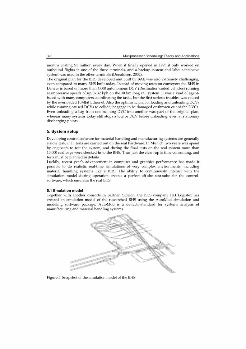
Multiprocessor Scheduling: Theory and Applications 390
months costing $1 million every day. When it finally opened in 1995 it only worked on outbound flights in one of the three terminals, and a backup-system and labour-intensive system was used in the other terminals (Donaldson, 2002). The original plan for the BHS developed and built by BAE was also extremely challenging, even compared to many BHS built today. Instead of moving totes on conveyors the BHS in Denver is based on more than 4,000 autonomous DCV (Destination coded vehicles) running at impressive speeds of up to 32 kph on the 30 km long rail system. It was a kind of agent-based with many computers coordinating the tasks, but the first serious troubles was caused by the overloaded 10Mbit Ethernet. Also the optimistic plan of loading and unloading DCVs while running caused DCVs to collide, baggage to be damaged or thrown out of the DVCs. Even unloading a bag from one running DVC into another was part of the original plan, whereas many systems today still stops a tote or DCV before unloading, even at stationary discharging points.
5. System setup
Developing control software for material handling and manufacturing systems are generally a slow task, if all tests are carried out on the real hardware. In Munich two years was spend by engineers to test the system, and during the final tests on the real system more than 10,000 real bags were checked in to the BHS. Thus just the clean-up is time-consuming, and tests must be planned in details. Luckily, recent year’s advancement in computer and graphics performance has made it possible to do realistic real-time simulations of very complex environments, including material handling systems like a BHS. The ability to continuously interact with the simulation model during operation creates a perfect off-site test-suite for the control-software, which emulates the real BHS.
5.1 Emulation model
Together with another consortium partner, Simcon, the BHS company FKI Logistex has created an emulation model of the researched BHS using the AutoMod simulation and modeling software package. AutoMod is a de-facto-standard for systems analysis of manufacturing and material handling systems.
Figure 5. Snapshot of the emulation model of the BHS

Decentralized scheduling of baggage handling using multi-agent technologies 391
One of the strong advantages of using AutoMod is that you can communicate with the model over a standard socket connection, which is almost identical to the connection between the control server and the PLCs in the real hardware. Thus the control software cannot see the difference, if it is connected to the emulation model or the real hardware. The same protocol and telegrams are used, which simplifies the development process, and makes the emulation model reliable, whenever the basic communication has been tested correct. A snapshot of the emulation model is shown in figure 5. It shows the area with input facilities for terminal 3 of the airport.
5.2 Agent platform
As already mentioned at the end of section 3, JADE has been chosen as the agent platform for the researched BHS. Firstly because JADE is FIPA compliant, it is well documented, continuously updated, and among the most reference agent platforms. In our setup the agents are still virtual collaborating processes running in a single JADE container on a single computer due to performance reasons1.
6. Agent design
In this section we will in details describe the tasks of the different elements in the BHS, which will form the final strategies we have applied to control the BHS. The elements are the building block of the BHS and from an intuitive point of view the potential candidates for agents in the system, as all actions of the system are performed by the elements. A classic approach of software engineering methods would lead to a functional decomposition, such as one agent for scheduling, another for resource management, etc. (Parunak, 1999), which is appropriate for centralized systems, but inspired from natural distributed systems Parunak also evinces that a physical decomposition of manufacturing systems into an agent model is both obvious and appropriate (Parunak, 1997). Our approach to model the system concentrates on the reasoning part of agents and their interaction. Following the notion of holonic agents by Ma ik & P chou ek, the holon part of the agent is packed into logic of the emulation model, but no special attention was given to comply with the IEC standard, which would modify the existing hardware. An alternative approach would be to consider the totes as “consumer” agents and the BHS as a collection of “producer” agents, as the BHS can solve the tasks that the totes want to have performed - bringing the tote to the destination. In principle a tote could then negotiate its way through the system, and if the bag was urgent it would be willing to pay a higher price than non-urgent bags. This approach often leads to other complications, such as communication overhead and complex agent management (Brennan & Norrie, 2003). Because the BHS generally consists of pathways of FIFO queuing lanes with little and often no possibilities of overtaking it is more appropriate to design the agents around the flow of the BHS, which makes the elements the potential candidates for agents alone. The element agents should then coordinate their activities to optimize system performance and should therefore be considered as collaborative agents, rather than competitive agents.
1 There is a huge overhead, when communicating across different agent containers or even worse when
communicating across different JAVA JVMs.

Multiprocessor Scheduling: Theory and Applications 392
6.1 Toploader
The input facilities of the BHS are called toploaders, as they drop bags into the totes from a conventional conveyor belt, see figure 6. Before the bag is inducted into the tote it is has passed a scanner, which reads its id and destination that are coupled with the tote, so the control system has exact tracking of the bag at all time. Identity and destination of the bag are unknown until the bag passes the scanner at the toploader shortly before being inducted if a tote is ready. The scanning initializes routing of the tote, but the short time leaves no option for global optimized planning of all current totes, and replanning when the next arrives.
Figure 6. A toploader, where bags arrive on a traditional conveyor belt
Basically the task of the toploader could be decomposed into scanning of the bag, which happen automatically and have no direct impact on the control. Secondly it initiates the journey of the tote on the BHS. In order to start the routing of the tote, the end-point (discharger) must be set for the tote. In order to optimize the capacity several dischargers are often allocated to the same flight destination2. Therefore the toploader agents initiate a negotiation with the possible dischargers to find the best suited discharger, the evaluation of the proposals from the dischargers is not trivially chosen as the lowest offer, but weighted with the current route length to the dischargers, which the toploader requests from a route agent - a mediator agent with a global focus on the dynamic route lengths of the BHS. The toplader can take two different approaches for routing the tote:
• Routing by static shortest path: After the toploader has decided on the discharger it could instruct all diverting elements along the route to direct that specific tote along the shortest path. Then the agent system would in principle work as the traditional control system by sending all totes along predefined static shortest routes3.
• Routing on the way: Instead of planning the entire route through the BHS, the toploader could just send the tote to the next decision point along the shortest route. A more dynamical and flexible approach, as the tote can be rerouted at a decision point if the route conditions have change, perhaps another route have become the dynamical shortest one, or the preferred discharging point have changed.
2 Due to the stopping of totes while unloading, the discharger has a lower line capacity than straight
elements. 3 In the researched BHS the decision between the alternative dischargers would also be predefined in
the conventional control. The BHS is built in layers to minimize cost and maximize space utilization, and alternative dischargers are always split on different layers, and the control system would try to avoid switching layers.

Decentralized scheduling of baggage handling using multi-agent technologies 393
6.2 Straight elements
Most of the elements of a BHS are naturally straight or curved elements that connect the nodes of the routing graph. Straight or curved elements are not considered as agents in our current design, because mechanically they will always forward a tote to the next element if it free, thus there are no decisions to be made. In principle the speed of each element could be adjusted to give a more smooth flow and avoid queuing, so one could argue that these decisions should be taken by the element itself. In the current setup it would generate an enormous communication overhead, because each element should be notified individually and the agents should be very responsive to change the speed in order to gain anything from speed adjustments.
6.3 Diverters
When straight elements are not considered as agents, divert elements becomes the first natural decision points on the routes. A diverter splits a conveyor lane into two, either a left or right turn and straight ahead. Lifts and so-called cross-transfers could be considered as special editions of the diverters. The cross-transfer allows the tote to be forwarded in all four directions.
Figure 7. A diverter element with an empty oversize tote
In respect to the strategies described above the diverter would either just forward the tote in the direction determined by the toploader, or it should reconsider alternative routes by restarting the negotiation process with dischargers and requesting updated information on dynamic route lengths. A diverter should be concerned about the relevancy of reconsidering the route for a tote, because in many cases there is only one possible direction at a given diverter for a given tote. We want to generalize the control logic of the diverter agents instead of customizing it according to the placement of the diverter in the BHS layout. Thus initially it adjusts itself to different destinations based on static route information. As mentioned for many diverters there are no alternative direction, for some the decision will have little impact, e.g. if the tote is close the discharger and there is little difference in dynamical route length between the two directions. For a few diverters the decision would have great impact on future decisions. That is mainly diverters placed at the points in the BHS, where it is possible to change layers4. Basically it is only important to reconsider the alternative dischargers at this point, because due to the layout of the BHS it is not possible to switch back to the other layer again, before the dischargers have been passed.
4 BHS is constructed as two layers of conveyor to save both space and cost.

Multiprocessor Scheduling: Theory and Applications 394
That leaves us with decision logic rather identical to the dynamic routing principle at toploaders, but diverters should fine-tune their decisions according to the local environment in which they are situated. In other words a strong influence on the decision logic of the diverter is based on its position in the routing graph.
6.4 Mergers
Mergers are the opposite of diverters, as they merge two lanes. Traditionally mergers are not controlled, as there are no alternatives to continuing on the single lane ahead, and the merger simply alters between taking one tote from either input lane, if both are occupied. Obviously, more intelligent decisions could be considered than just switching between the input lanes, which is the argument for applying agents to the merger elements. The ratio between merging totes from the input lanes should be determined by the aggregated data of the totes in either of the two lanes. E.g. if the number of urgent totes waiting to be merged are higher in one lane that lane should be given higher priority. Also waiting totes in one lane could have greater impact on the overall system performance, if a queue of totes in one lane is more likely to block other routes behind that point.
6.5 Dischargers
Dischargers are responsible for unloading bags from the totes, when the tote reaches its destination. When bags are discharged they fall onto carrousels similar to those at baggage claim and are drown to the plane in small wagon trains.
Figure 8. A discharger element that can tilt the tote, so bags slide onto the conveyor belt
Besides being involved in the negotiation process described for the toploaders, the task of the discharger could seem rather simple - just tilting the tote, but a discharger also has to take care of the empty totes. Some BHSs have separate conveyor system for the empty totes, but many systems including the researched BHS use the same lanes for routing the empty totes back to the tote stackers at the toploaders. The task of routing empty totes is similar to routing full totes at the toploaders, but actually much more complex, due to a number of considerations that must be taken into account.
• The number of destinations (tote stackers) is larger than alternative dischargers for full totes (typically 2), whereas the number of tote stackers is equal to the number of toploaders, which is 12 in our case.
• Specially in the input area, empty totes are mixed with full totes and the area could easily get overloaded and blocked.

Decentralized scheduling of baggage handling using multi-agent technologies 395
• During peak times it should be considered sending some empty totes to temporary storage in the EBS area, which is far from the input area, and released again when the load on the system is lower.
• The status of empty tote stackers. If a stacker runs empty, no totes will be available at the toploaders for new bags.
• The distance to the stackers. It is more appropriate to return the empty tote to a stacker nearby than sending it half way through the system.
All factors should be considered and measured against a fuzzy set, which are weighted to an aggregated value - a proposal of a bid plan to go to each of the stackers.
6.6 EBS elements
Early baggage storage elements, or EBS for short, are temporary storage elements for totes with bags for which a discharger has not been allocated yet, as described above when defining the concept of rush-bags.
Figure 9. EBS elements, here storing a line of empty totes
It is a complete research area for itself to optimize the utilization of the EBS, as totes are stored in lanes, which are released into the system again, but planning and coordinating the totes in different lanes is not a simple task, but will not be given further attention in this chapter.
7. Agent interactions and ontology
As mentioned in section 3 FIPA has not yet approved specifications and guidelines for agent applications in the manufacturing domain. Thus we have developed the agent interactions based on the elements responsibility and participation in the function of the BHS, as described in the previous section. Due to both time constraints and focus of the DECIDE project, it was never an issue to change the setup of the hardware. The layout of the BHS was determined in advance of the project, and research goals were to investigate if multi-agent based control software could replace traditional control structures in an efficient way.
7.1 Adapter Agent
Given the setup, where the agents resides as virtual representations of their corresponding elements in a container of the JADE platform, and the actions of the agents are visualized in the emulation software, we required a gateway agent to handle the communication protocol. This agent was named AdapterAgent and could be understood as a converter of stimuli and action messages between the agent community and the real world or hardware,

Multiprocessor Scheduling: Theory and Applications 396
which in our setup is represented by the AutoMod model. The interface between the AutoMod model and the AdapterAgent follows the same protocol and telegram structure as the interface to the real hardware. The AdapterAgent constantly listen for new telegrams from the AutoMod model. Thus it encapsulates the entire perception of the whole agent community towards the environment, the notifications received from the model are converted to agent messages complying with the FIPA ACL specification and message contents are encoded with the ontology we have defined for the BHS domain. The AdapterAgent is not thought to be a filter of the message exchange, thus all information from the model is encoded into the messages and forwarded to interested agents, and no notifications are omitted. Ideally all agents would be connected to the model, and communicate directly with their corresponding element, but that would require more than 300 concurrent threads listening on their own socket connection to the model, which is inappropriate for performance reasons. Thus perception has been extracted and isolated into the AdapterAgent, in order leave the element agents with a natural external interface they subscribe to interesting messages from the AdapterAgent. It is not the task of the AdapterAgent to figure out, where to send messages. During initialization all element agents initiate a subscription for each of the emulator notifications they are interested in. The negotiation of subscriptions follows the FIPA subscription specification, but subscriptions are always approved. Because no handshaking is defined for communication with the model, all message sent from the AdapterAgent are inform messages with no expectation of agree or accept replies. That also has the positive side effect that the AdapterAgent is not required to understand the messages (except simple conversation) and couple a response to a notification. Element agents are fully responsible for replying if require. Exactly the same apply in the opposite direction as well (no coupling between commands or queries to the model and the replies), thus inform message are a natural choice.
7.2 Mediator agents
There is a balance between giving agents detailed information about the environment and maintaining an internal world model, or let them query the environment about information when required. The FIPA Directory Facilitator is a strong tool when dynamically searching the environment for appropriate services. It is used when dischargers are allocated to a flight, they register a new service for that departure in the DF and agents requesting a flight can simply search the DF, instead holding information about all dischargers. That is a quite trivial use of the yellow page service of the DF. In theory the service and discovery approach could be used to route totes around in the system to fully decouple agents from physical connections, but that would generate too much overhead and complicate the simple routing principles. Instead agents can be assisted by mediator agents, who collect aggregated information for the entire system. The RouteAgent is an example of such an agent. In the initialization process the RouteAgent generates all possible routes in the system by building up a graph for the BHS with nodes corresponding to the element agents. During operation it constantly monitors traffic on edges of the graph by subscribing to such information in the AdapterAgent and update the weights in the graph, so dynamic shortest paths can be calculated using classic Dijkstra for dynamic shortest path calculations (Dijkstra, 1959).

Decentralized scheduling of baggage handling using multi-agent technologies 397
Following the FIPA query-ref communication act element agents can request routes to a given destination packed in a referential expression of the query message. The referential expression is composed using the ontology we have defined for the BHS domain, which extends and follows the structure of the FIPA-SL. The RouteAgent understand two concepts of the ontology, RouteBetween and LineBetween:
• RouteBetween is the concept used, when agents are interested in full or parts of a route, but only with a granularity of finding other element agents along the path – only information on nodes of the graph are returned.
• LineBetween is the fine-grained concept providing all details about a conveyor line of connected elements in the BHS – information about edges between two given connected nodes.
To give an example of the generality embedded in ontology-based messages, a query to the RouteAgent could contain the following abstract referential expressions:
(iota:Variable (Variable :Name x :ValueType set) :Proposition (routeBetween
:origin (element :elementID DFB01.TLA001) :destination (element :elementID DLA02.DIA023) :viaPoints (Variable :Name x :ValueType set) :numNodes 0
))
Abstract because it contains the variable x that must be replaced by the responder in a response to the query. In this case a set of points (id’s of element agents between the given origin and destination). The predicate iota is just one of three from the FIPA-SL specification, which means exactly one object that fulfils the expression, whereas the other predicates, anyand all, would return any or all routes between the origin and destination, respectively. The approach of the RouteAgent was not only taken to omit the world model in the element agents, but also to support a simple implementation of the basic approach of the traditional control software to compare against the agent-based solution. In current and future experiments conducted on the BHS we try to exclude the RouteAgent by giving elements agents a dynamic profile of their local environment, which is further described in under future work, because it simplifies agent interactions.
7.2 Routing negotiations
The negotiation and collaboration interactions framing the simple routing principle in the BHS, have been selected to give an illustration of how the interoperability among agents are achieved using normative FIPA specifications. The toploading and routing principle are described in general terms in the beginning of section 6. It is also mentioned that the inter-agent communication is almost identical at both toploaders and diverter, when we deal with dynamic routing – in case of routing along static shortest path, the toploader simply make all the decisions and informs all diverters along the route how to direct the tote. The toploader receives a stimuli by means of an inform message from the AdapterAgent that a new bag has been scanned. Assuming no problems the toploader searches the DF for discharge agents that have been allocated to the destination of the bag revealed in the

Multiprocessor Scheduling: Theory and Applications 398
scanned code of the bag. If no discharger are available the bag will be routed to the EBS, otherwise the toploader will initiate a FIPA contract net with the dischargers to collect proposals of accept for the new bag. Concurrently the toploader request route information to the dischargers from the RouteAgent, where route lengths are combined with the proposals from the dischargers to take the final decision of the best discharger for the bag. Shortly after the first stimuli from the AdapterAgent the toploader will receive another stimuli from the model that the bag has been inducted into the tote and the tote is released from the toploader. This inform message purely serves the purpose of combing the scanned bag id (the IATA tag) with the tote id, so routing can be handled correctly for the rest of the journey. In case of the static routing principle the toploader send FIPA request messages to all node agents along the route with an action request to direct the tote in the given direction, when it is seen at the node. This approach purely violates the autonomy of those agents, but as mentioned above it primarily serves the purpose of comparison. Figure 10 illustrates the interactions in a simplified sequence diagram.
Figure 10. Example of agent interoperability
As outlined above all communication follows the FIPA specifications in order to generalize the interoperability among agents and increase the possibility of reuse. The content of the messages are encoded in abstract task descriptions or status reports from the individual element agents, again to minimize the influence of application domain.
8. Internal agent reasoning
The previous section dealt with agent interoperability and the communication design in respect to the FIPA specification. As stated in section 3 FIPA is only concerned with the external behaviour of the agents, but the internal behaviour of agents and the reasoning part is also of extreme importance.

Decentralized scheduling of baggage handling using multi-agent technologies 399
In this section we will present internal agent reasoning principles to optimize the flow in the BHS in different ways to meet some of the performance parameters. Deep reasoning and long-term goals are not currently pursued in the strategies, due to the flow speed and high number of totes in the system. Instead the intensions behind the strategies are to optimize the situation for more than a single tote or forthcoming actions. We will give examples of three different deliberate behaviours, which take part in both necessary routing and optimizing strategies for the BHS.
8.1 Returning empty totes
As explained in section 6.5 the task of dischargers is more complicated than just emptying the tote. The tote continues on the conveyors and should be routed back to tote stackers located at the input facilities. We currently omit the EBS logic from the control software (no arriving bags will have more than 3 hours to departure), so we do have to consider temporarily storing empty totes in the EBS area. The most important factor that influences the decision of where the empty tote should be returned to, is the full status of the tote stackers, but also the distance to the tote stackers should be considered. There is no reason to send it to the other end of the system, if a stacker is nearby, unless the other is empty. Each stacker monitors its full status as a simple ratio between the current and maximum number of totes in the stacker. By a standard indeed fuzzy hedge (Negnevitsky, 2005) the
ratio is converted into a priority is for requesting extra totes.
≤≤−−<≤
=1)1(21
02
212
212
ii
iii rr
rrs (1)
where ir is the full-ratio for the i 'th stacker. A plot of the function is shown in figure 11.
Figure 11. Plot of ETS priority function
The priority determined is used to scale the dynamic route length to each tote stacker, so a nearly empty stacker will have a very short route length or value in the decision, whereas a full stacker will have its full route length.
iii sdv ⋅= (2)
where id is the dynamic distance (requested from the RouteAgent) to the stacker from the
decision point. This behaviour clearly serves our purpose of refilling the empty tote stackers at the input facilities, but the importance of correct routing will be far more interesting when the EBS area is included in the agent system. For the discharger the EBS could be considered as just another destination (stacker) that never runs full in practice, but in the long run it generates extra traffic to send the tote back via the EBS area.

Multiprocessor Scheduling: Theory and Applications 400
8.2 Overtaking urgent bags
Consider a typical layout of a discharging area in figure 12. The bottom lane is a fast forward transport line, the middle a slower lane with the dischargers and the upper lane is the return path. A diverter (in the bottom lane) has the option to detour non-urgent to the middle lane to give way for urgent baggage in the transport line, but with no queues in the system all totes should follow the shortest path. When the routes merge again at the mergers in the middle lane, it will give higher priority to totes from the merging leg with the most urgent baggage.
Figure 12. Area of the BHS layout with indication of diverters, mergers, and dischargers
Urgency is a constructed function, which gives high priority to urgent totes and negative priority to totes, where remaining time to departure exceed a threshold.
≥−+−−
<=
TjTjTjT
Tjj
j
UtUtUtUU
Uttu
)2()(
1
1
22
2max
2
(3)
where maxU is the full window size of the allocated discharger. If the tote’s remaining time
exceed this value it should go to EBS. TU is the threshold value, which is set to 20 min, as no
tote should be considered urgent, if it has more than 20 min left before the discharger
closes5. jt is the remaining time for the j 'th tote. The graph is plotted in figure 13.
Figure 13. Urgency function for totes
The urgency factor is converted to a scale factor for the dynamic route lengths of alternatives routes. Then the principle of simple modification of the route lengths can be used here as well.
≥−−−<+−
=+
+
tote)(urgent0)1)(1(
)toteurgentnon(0)1)(1(
1
1
jkj
jkjj uvu
uvus (4)
where 1+kv is the aggregated urgency value for the next decision point along the route, which is
requested in a communication act (FIPA request-ref) to the divert agent. The formula secures that
5 When the discharger closes the tote becomes a rush-bag, but the threshold of 20 minutes is
independent of the 20 minutes time limit for rush bags, described in section 4.1, so in total a tote is considered non-urgent if it has more than 40 minutes left to departure.

Decentralized scheduling of baggage handling using multi-agent technologies 401
urgent totes will group along the shortest route (as 1+kv is close to 1), whereas non-urgent are
punished along the detour. If there are no queues on the routes the 1+kv is 0, and the scale factor
has no effect. The mergers in the middle lane simply give higher priority to input lanes with more urgent totes. The ratio between the aggregated urgency factors of the input lanes becomes the ratio for merging totes from the input lanes.
8.3 Saturation management
Another important strategy is trying to avoid queues at all by minimizing the load on the system in critical areas. We assume everybody is familiar with slow starting queues of cars at an intersection, when the light turns green. Acceleration ramps and reaction times relative to drivers ahead accumulate to long delays in traffic queues, even though in theory all drivers should be able to accelerate synchronously (no reaction time). The same problem arises in the BHS, where reaction times correspond to the delay of the element head reporting clear6. These matters result in the characteristics of the work in-progress against capacity curve (WIPAC), which is further described in (Kragh, 1990) that states the capacity of a system goes dramatically down, if the load on the system exceed a certain threshold value, as indicated in the figure 14.
Figure 14. Theoretical WIPAC
The curve is dynamical, due to the various and changing load on the system, and the maximum cannot be calculated exactly. Thus the strategy is to quickly respond to minor observations, which indicates that the maximum has been reached, and then block new inputs to the area. We call this approach for saturation management, and currently we block a toploader if the routes from the toploader are overloaded. Queues close to the toploader are most critical, as the toploader have great impact on filling up those queues, whereas the parts of the route far from the toploader could easily have been resolved before the new totes arrive. Instead of blocking the toploader completely, we can just slow down the release of new totes using the following fraction of full speed for the toploader.
==
ii
i ii
i i
i iit
d
qd
wqw
v α
α
(5)
6 In the mechanical setup of the BHS a tote can only be forwarded from one conveyor element to the
next element, if that element is clear. A synchronized row of totes can then pass at full speed, from one element to another, but in queue situations acceleration ramps delays each element.

Multiprocessor Scheduling: Theory and Applications 402
where tv is the full speed of the toploader, and iw are weights of the queue statues, iq , along
the routes. The weight is given by a fitted coefficient, α , and the distance from the toploader
id . Queue statuses, iq , are always a number between 0 and 1, where 1 indicates no queue.
The effect of the saturation management strategy is clearly documented by the graph in figure 15. Thus the decision taken by the toploader agent is highly dependent on the current configuration of the environment around the toploader.
Figure 15. Result of a test scenario with and without the saturation management strategy
9. Conclusion
Is this chaper we have presented novel research contributions from an application project under the DECIDE project that deals with multi-agent based control in production systems. In this case a baggage handling system (BHS) in a major airport hub in Asia. Agents were intended to substitute existing control logic, but not change the layout of the BHS. Interoperability of the agents have been secured through the use of FIPA specifications, which generalized the design of the agents to be applicable for other material handling systems. We have succeeded in keeping the decision logic of the agents rather general in order to improve reusability and understandability for the agent based control. Special attention has been given to the task of the different type of agents, and examples of implemented decision logic have proven successful compared to the traditional approach.
9.1 Future work
We continue our research on the BHS and will develop more new strategies for the local agents, and increase their mutual collaboration to maximize the utilization of the BHS during peak times. We will try to avoid the use of centralized mediator agents (the RouteAgent) and rely on roles and profiles for the agents. Ideally a swarm of local agents would provide the most general setup, which easily can be ported to other manufacturing and material handling systems. During the research we will pay special attention to develop abstract and general design methodologies for the topological domain of impact for agent collaborations.
9.2 Acknowledgements
We would like to thank all the participants in the DECIDE project, which is supported by the The Ministry of Science, Technology and Innovation in Denmark. A special thank to FKI Logistex (http://www.fkilogistex.com) and Simcon (http://www.simcon.dk) for their support, feedback, and creation of the AutoMod model of the major hub airport.

Decentralized scheduling of baggage handling using multi-agent technologies 403
10. References
Brennan, R. W. & Norrie, D. H (2001). Agents, holons and function blocks: distributed intelligent control in manufacturing. Journal of Applied Systems Studies Special Issues on Industrial Applications of Multi-Agent and Holonic Systems, Vol. 2, No. 1, 2001, pp. 1-19.
Brennan, R. W. & Norrie, D. H (2003). From FMS to HMS, In: Agent-Based Manufacturing – Advances in the Holonic Approach, Deen, S. M., (Ed.), pp. (31-49), Springer, ISBN 3540440690, Berlin, Germany.
Brückner, S.; Wyns, J.; Peeters, P. & Kollingbaum, M. (1998). Designing Agents for Manufacturing Control. Proceedings of the 2nd Artificial Intelligence and Manufacturing Research Planning Workshop, pp. 40-46, Albuquerque, August 1998.
Bussmann, S. (1998). An agent-oriented architecture for holonic manufacturing control. Proceedings of First Workshop on Intelligent Manufacturing Systems Europe, pp. 1-12, Lausanna, Switzerland, 1998, EPFL.
Bussmann, S. & Schild, K. (2001). An Agent-based Approach to the Control of Flexible Production Systems, Proceedings of 8th IEEE Int. Conf. on Emerging Technologies and Factory Automation (ETFA 2001), pp. 169-174, Antibes Juan-les-pins, France.
Christensen, J. H. (1994). HMS: initial architecture and standard directions, Proceedings of the 1st European Conference on Holonic Manufacturing Systems, pp. 1-20, HMS Consortium, Hannover, Germany.
Decker, K. (1995). Environment Centered Analysis and Design og Coordination Mechanisms, Ph.D. thesis, Department of Computer Science, University of Massachusetts, May 1995.
Decker, K. & Li, J. (1998). Coordinated Hospital Patient Scheduling, Proceedings of the Third International Conference on Multi-Agent Systems (ICMAS98), pp. 104-111, IEEE Computer Society, Washington, DC, USA.
Decker, K. & Li, J. (2000). Coordinating Mutually Exclusive Resources using GPGP. Autonomous Agents and Multi-Agent Systems, Vol. 3, No. 2, pp. 133-157, Springer.
Di Caro, G. & Dorigo, M. (1997). AntNet: A Mobile Angents Approach to Adaptive Routing.Université Libre de Bruxelles, IRIDIA/97-12, Belgium.
Dijkstra, E. W. (1959). A Note to Two Problems in Connexion with Graphs. Numerische Mathematik, Vol. 1, pp. 269-271.
Donaldson, A. J. M. (2002). A Case Narrative of the Project Problems with the Denver Airport Baggage Handling System (DABHS). Middlesex University, School of Computing Science, TR 2002-01, January 2002.
FIPA (2002a). FIPA Abstract Architecture Specification. Foundation for Intelligent Physical Agents, SC00001L, December 2002.
FIPA (2002b). FIPA Communicative Act Library Specification. Foundation for Intelligent Physical Agents, SC00037J, December 2002.
Flake, C.; Geiger, C.; Lehrenfeld, G.; Mueller, W. & Paelke, V. (1999). Agent-Based Modeling for Holonic Manufacturing Systems with Fuzzy Control, Proceedings of 18th
International Conference of the North American Fuzzy Information Processing Society (NAFIPS'99), pp. 273-277, June 1999, New York, USA.
Giret, A. & Botti, V. (2005). Analysis and Design of Holonic Manufacturing Systems, Proceedings of 18th International Conference on Production Research (ICPR2005).
Gufflet, Y. & Demazeau, Y. (2004). Applying the PACO paradigm to a three-dimensional artistic creation, Proceedings of 5th International Workshop on Agent-Based Simulation (ABS'04), pp. 121-126, May 2005, Lisbon, Portugal.
Multiprocessor Scheduling: Theory and Applications 404
Koestler, A. (1967). The Ghost in the Machine, Penguin, ISBN 0140191925, London, United Kingdom.
Kragh, A. (1990). Kø-Netværksmodeller til Analyse af FMS Anlæg. Ph.D. thesis, Informatics and Mathematical Modelling, Technical University of Denmark.
Maionea, G. & Naso, D. (1996). A soft computing approach for task contracting in multi-agent manufacturing control. Computers in Industry, Vol. 52, No. 3, pp. 199-219.
Ma ik, V. & P chou ek, M. (2001): Holons and agents. Recent developments and mutual impacts, Proceedings of the Twelfth International Workshop on Database and Expert Systems Applications, pp. 605-607, IEEE Computer Society.
Ma ik, V.; P chou ek, M.; Vrba, P. & Hrdonka, V. (2003). FIPA Standards and Holonic Manufacturing, In: Agent-Based Manufacturing – Advances in the Holonic Approach,Deen, S. M., (Ed.), pp. (31-49), Springer, ISBN 3540440690, Berlin, Germany.
Negnevitsky, M. (2005). Artificial Intelligence – A Guide to Intelligent Systems, 2. edition, Addison Wesley.
Parunak, H. V. D. (1987). Manufacturing Experience with the Contract Net, In: Distributed Artificial Intelligence, Huhns, M. N. (Ed.), pp. 285-310, Pitman Publishing, London.
Parunak, H. V. D. (1995). Autonomous Agent Architectures: A Non-Technical Introduction.Industrial Technology Institute, ERIM, 1995.
Parunak, H. V. D. (1996). Applications of Distributed Artificial Intelligence in Industry, In: Foundations of Distributed Artificial Intelligence, O’Hara, G. & Jennings, N. (Ed.), pp. 139-163, Wiley Interscience, ISBN 0471006750, New York, USA.
Parunak, H. V. D. (1997). “Go to the Ant”: Engineering Principles from Natural Multi-Agent Systems. Annals of Operation Research, Vol. 75, pp. 69-101.
Parunak, H. V. D. (1999). Industrial and Practical Applications of DAI, In: Multiagent Systems – A Modern Approach to Distributed Artificial Intelligence, Weiss, G. (Ed.), pp. 377-421, MIT Press, ISBN 0262232030, Cambridge, MA, USA.
Sandell, N.; Varaiya, P.; Athans, M. & Safonov, M. (1978). Survey of decentralized control methods for large scale systems. IEEE Transactions on Automatic Control, Vol. AC-23, No. 2, April 1978, pp. 108-128, ISSN 0018-9286.
Schoonderwoerd, R.; Holland, O.; Bruten, J. & Rothkrantz, L. (1996). Ant-Based Load Balancing in Telecommunication Networks. Adaptive Behaviour, No. 5, 1996, pp. 169-207.
Searle, J. R. (1969). Speech Acts, Cambridge University Press, ISBN 052109626. Sipper, D. & Bulfin, R. (1997). Production: Planning, Control and Integration, McGraw-Hill
College, ISBN 0070576823. Swamidass, P. M. (1988). Manufacturing Flexibility, Monograph No. 2, Operations
Management Association, Texas, USA. Taylor, F. W. (1911). The principles of scientific management. Harpers & Brothers Publishers,
ISBN 048629980, New York, USA. Willliamson, D. (1967). System 24 – a new concept of manufacture, Proceedings of the 8th
International Machine Tool and Design Conference, pp. 327-376, University of Manchester, September 1967, Pergamon Press, Oxford.

22
Synchronized scheduling of manufacturing and 3PL transportation
Kunpeng Li1 and Appa Iyer Sivakumar2
1School of Management, Huazhong University of Science and Technology 2Singapore-MIT Alliance, School of Mechanical and Aerospace Engineering, Nanyang
Technological University 1P.R. China, 2Singapore
1. Introduction
Many companies are enhancing their competitiveness by offering Just-in-Time (JIT) delivery. Costs or penalties are incurred by delivering an order either earlier or later than the customer’s due-dates. Besides, maintaining short response time from order acceptance to final delivery is one of the key competitive advantages. Thus, many companies deliver products to customers directly after production without holding finished product inventory. This is particularly true for the industries with short product life cycle, such as consumer electronics manufacturing, ready-mix concrete supplying and food catering industry (Garcia et al. 2004; Chen and Vairaktarakis, 2005; Li et al., 2005). In order to improve customer service and reduce production and transportation costs, scheduling of assembly manufacturing and transportation should be synchronized. Nowadays, due to the professional services provided by third party logistics (3PL) provider, it is more efficient to outsource the transportation or distribution to 3PL. There are two types of operations. If 3PL only serves one customer, the schedule of 3PL’s vehicle is determined by the order completion time in manufacturing. This type of operation is particularly true for 3PLs that providing road transportation services. On the hand, if 3PL provides services to more than one manufacturer, the departure and arrival time of the vehicle is determined by 3PL rather than by the manufacturer. In addition, the unit transportation cost of each vehicle varies. The manufacturer can book capacity on the available vehicles accordingly. Then, decision on allocation of orders to the vehicles is made to utilize the booked capacity efficiently. The typical case is the air-cargo transportation service provided by cargo airlines. Motivated by above application, this chapter studies the problem of synchronized scheduling of assembly manufacturing and transportation in the make-to-order (MTO) consumer electronics supply chain (CESC). In this context, materials or components are kept in inventory before assembly. Upon reception of customer orders, the materials are transferred to manufacturing job shop. Through several processes such as assembly, testing, packing, the assembly manufacturing is completed. Then, the order is transported to customers directly by the vehicle of 3PL. Chen and Vairaktarakis (2005) addressed the integrated production transportation scheduling problem considering the first type of 3PL

Multiprocessor Scheduling: Theory and Applications 406
operations, which is mentioned above. Conversely, the second type of 3PL operations is considered in this chapter. The objective of this problem is first to determine appropriate allocation of orders to available vehicle capacities to minimize total delivery cost which consists of transportation cost, delivery earliness penalty cost and delivery tardiness penalty cost. The allocation is constrained by production capacity. In other words, manufacturing of orders should be completed before the departure time of the vehicle that the order allocated to. Then, the schedule of assembly manufacturing is determined to make sure that each order is completed on time, while the order waiting time before transportation is minimized. According to Li et al. (2005), the solution method consists of two phases. A network representation of the two stage decision model is shown in Figure 1.
flight 1
......
flight 2
flight n
Assembly
manufacturing flow
shop
orders
Customer
Figure 1. Two stage decision model in CESC
In the first phase, the proposed Integer Linear Programming (ILP) model will run for the transportation issues of the outbound logistics assuming that the number of completed-customers'-orders are available and the production rate of assembly manufacturing is fixed and known. In the second phase, using the above optimal decision obtained for the outbound logistics, i.e., the flight wise customers' orders movement strategy, an efficient release control policy is decided for the assembly manufacturing based on the available assembly capacity. The 3PL transportation allocation problem and the assembly scheduling problem formulated in this work are based on the following assumptions:
Decisions of transportation allocation and assembly scheduling are for the orders accepted in the previous planning periods.
All the packed products have same or similar dimensions.
Business processing time and cost, together with loading time and loading cost for each vehicle are included in the transportation time and transportation cost.
Vehicle departure time is taken as the time that 3PL’s vehicle set out from the manufacturer’s plant. Vehicle arrival time is taken as the time that the vehicle reaches customer.
Orders released into production facility for the planning period are delivered within the same planning period which means there are no production backlogs.
For assembly manufacturing, setup time is included in the processing time.
Assembly flow shop consists of single machine. The machine can process only one part at a time.
There are no machine breakdowns and preemptions.
Total manufacturing time of an order is directly proportional to the order’s quantity.

Synchronized scheduling of manufacturing and 3PL transportation 407
Waiting penalties for orders before transportation are order independent, i.e., they are not determined based on any job characteristics.
The starting time of the planning period is set equal to zero.
2. The 3PL Transportation Problem
The 3PL transportation problem is formulated using an Integer Linear Programming (ILP) model. As the air transportation is a typical case for the 3PL transportation, the 3PL transportation is represented by air transportation hereafter. The model allocates orders to the existing air transportation capacities with minimum costs. Synchronization is incorporated into the ILP model by including the constraint that balances the production rate of the assembly facility with the flight allocation. The following notation is defined: i = order index, i=1, 2, …. N; f, f’ = flight index, f=1,2,……F;k = destination index, k = 1,2,……L; Af = arrival time of flight f at the destination; Desi = order i’s destination; Desf = flight f’s destination; LN = a large number; |LN| = absolute value of LN;Qi = quantity of order i; di = due date of order i;Df =departure time of flight f at the local place where the manufacturing plant is located; NCf = transportation cost for per unit product allocated to normal capacity area of flight f;SCf = transportation cost for per unit product allocated to special capacity area of flight f;NCapf = available normal capacity of flight f;SCapf = available special capacity of flight f;
i = delivery earliness penalty cost (/unit/hour) of order i;i = delivery tardiness penalty cost (/unit/hour) of order i;
WTi = waiting time of order i between assembly and air transportation; PEif = per unit delivery earliness penalty cost for order i when it is transported by flight f,
PEif= Max(0,di - Af)* i (1)
PLif = per unit delivery tardiness penalty cost for order i when it is transported by flight f,
PLif= Max(0,Af - di)* i (2)
Zif = quantity of order i allocated to flight fXif = the quantity of the portion of order i allocated to flight f’s normal capacity area; Yif = the quantity of the portion of order i allocated to flight f’s special capacity area; PR = the production rate of assembly manufacturing; In case of split deliveries, an order can be split and delivered among any number of flights. The ILP model for the multi-destination air transportation problem is expressed as follows:
Minimize
i fifif
i fiffi
i fiff
i fiff ZPLZPEYSCXNC (3)
Subject to:
ififif ZYX , for all i, f (4)
1||** fiif DesDesXLN , for all i, f (5)
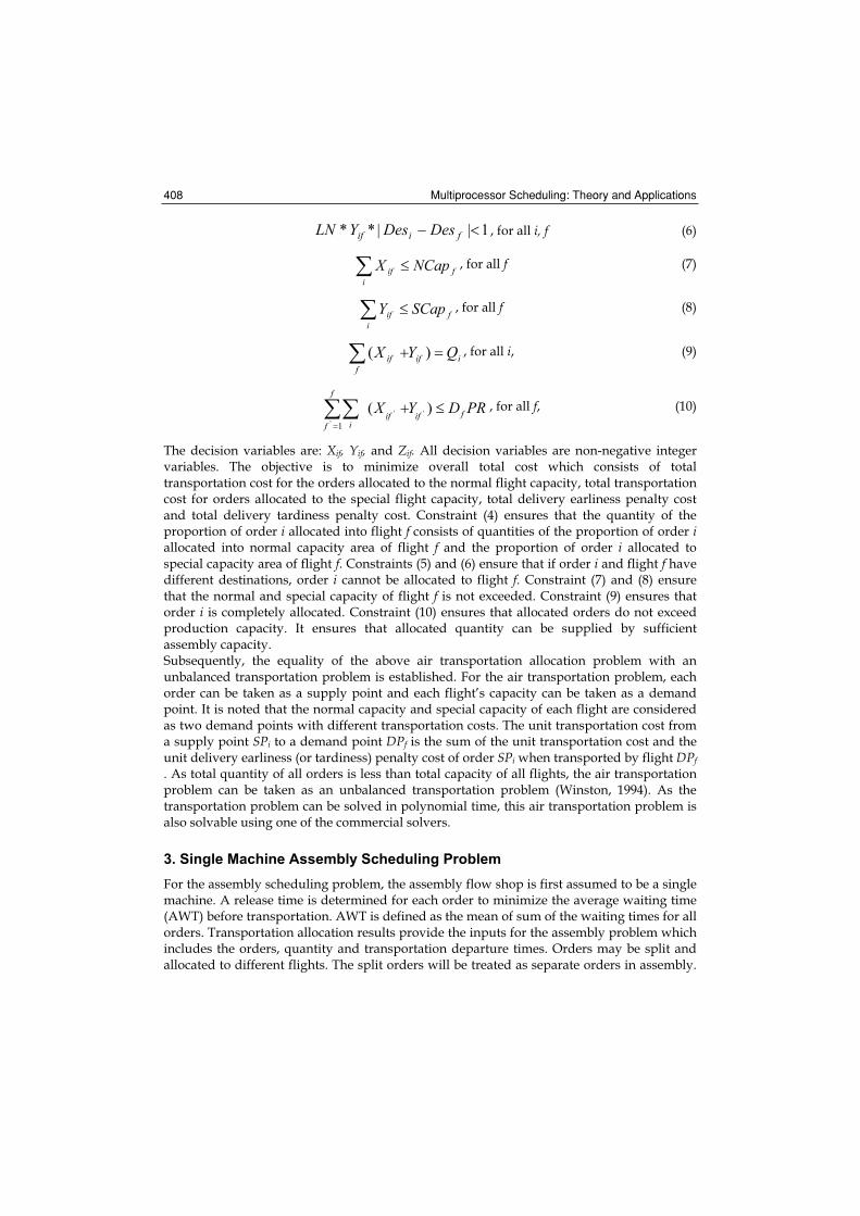
Multiprocessor Scheduling: Theory and Applications 408
1||** fiif DesDesYLN , for all i, f (6)
fi
if NCapX , for all f (7)
fi
if SCapY , for all f (8)
iiff
if QYX )( , for all i, (9)
, for all f, (10) PRDYX fif
f
fif
i)( '
'
'
1
The decision variables are: Xif, Yif, and Zif. All decision variables are non-negative integer variables. The objective is to minimize overall total cost which consists of total transportation cost for the orders allocated to the normal flight capacity, total transportation cost for orders allocated to the special flight capacity, total delivery earliness penalty cost and total delivery tardiness penalty cost. Constraint (4) ensures that the quantity of the proportion of order i allocated into flight f consists of quantities of the proportion of order iallocated into normal capacity area of flight f and the proportion of order i allocated to special capacity area of flight f. Constraints (5) and (6) ensure that if order i and flight f have different destinations, order i cannot be allocated to flight f. Constraint (7) and (8) ensure that the normal and special capacity of flight f is not exceeded. Constraint (9) ensures that order i is completely allocated. Constraint (10) ensures that allocated orders do not exceed production capacity. It ensures that allocated quantity can be supplied by sufficient assembly capacity. Subsequently, the equality of the above air transportation allocation problem with an unbalanced transportation problem is established. For the air transportation problem, each order can be taken as a supply point and each flight’s capacity can be taken as a demand point. It is noted that the normal capacity and special capacity of each flight are considered as two demand points with different transportation costs. The unit transportation cost from a supply point SPi to a demand point DPf is the sum of the unit transportation cost and the unit delivery earliness (or tardiness) penalty cost of order SPi when transported by flight DPf
. As total quantity of all orders is less than total capacity of all flights, the air transportation problem can be taken as an unbalanced transportation problem (Winston, 1994). As the transportation problem can be solved in polynomial time, this air transportation problem is also solvable using one of the commercial solvers.
3. Single Machine Assembly Scheduling Problem
For the assembly scheduling problem, the assembly flow shop is first assumed to be a single machine. A release time is determined for each order to minimize the average waiting time (AWT) before transportation. AWT is defined as the mean of sum of the waiting times for all orders. Transportation allocation results provide the inputs for the assembly problem which includes the orders, quantity and transportation departure times. Orders may be split and allocated to different flights. The split orders will be treated as separate orders in assembly.

Synchronized scheduling of manufacturing and 3PL transportation 409
The transportation departure time is taken as the due date of assembly for each order. The assembly schedules adhere to the following conditions: (i) each machine processes only one job at a time (ii) pre-emption is not allowed, which means once a job’s processing is started, it can not interrupted by another job and (iii) processing time of each order is known. Two methodologies for assembly scheduling problem are presented in this section.
3.1 Forward Synchronized Scheduling Heuristic (FSSH)
Normally in practice, the schedules constructed use dispatching rules and follow a forward dispatch method. Forward approach schedules jobs in a given sequence one by one, starting from the first job, to achieve feasible and compact schedules. The approach usually generates non-delay schedules. A non-delay schedule is one in which no machine is kept idle at any time when at least one job is waiting for processing. Longest Processing Time (LPT) rule is selected as the dispatching rule. LPT minimizes total earliness in single machine scheduling in the situation of no tardiness for jobs (Panwalkar et al., 1982). Since there may be split orders in allocation, the sequence determined by LPT rule may be adjusted to combine the split orders to facilitate assembly manufacturing while maintaining the transportation schedule of the split orders. The general scheme for FSSH is: Step 1: Group orders that are allocated to the same flight, and sequence the order groups by the rule of earliest flight departure time first. Step 2: Use LPT rule to sequence the orders within the each group. Step 3: Assembly batching of split orders (ABSO): This step is used to combine the split orders in a batch for assembly so that split orders in transportation can be treated as a whole order in assembly. This step is applied only in the situation when an order is split and allocated to two adjacent flights. The split orders are processed in sequence by scheduling them as last order for the first flight and first order for the second flight. This is to facilitate the assembly processing of an order. Step 4: Calculate each order’s release time by forward dispatch method starting from the first order to the last order. The first order’s release time equals zero. The release time of succeeding orders are obtained by adding the assembly processing time of their preceding ordersStep 5: Compute the AWT between assembly and transportation. The number of order groups in the planning period, corresponds to the number of flights that transport orders to the customer destinations, is determined by the transportation allocation model. Each order group consists of set of orders and they have same assembly due-date.
3.2 Backward Synchronized Scheduling Heuristic (BSSH)
Steps of BSSH are the same as FSSH except for step 4. Backward scheduling is used in step 4 in BSSH instead of forward scheduling in FSSH. Backward scheduling is reverse of the forward scheduling approach and schedules are defined on a reverse time frame. The start time and completion time of the same job in forward scheduling mode is related to the completion time and start time of the same job in backward scheduling mode. In other words, the completion time of each job is determined first. The release time (or start time) for each job is then obtained using the determined completion time. To arrive at a schedule after using backward scheduling approach, the

Multiprocessor Scheduling: Theory and Applications 410
processing sequence is reversed, and the schedule time frame is reversed back to forward time frame. The backward scheduling considers inserted idle times between processing of orders. Forward scheduling is a straightforward method that schedules jobs one by one from the beginning time of the planning period. The main objective is to make sure that each job can meet its due date. The forward scheduling methodology presented in the previous section does not minimize AWT effectively. This is overcome by adopting a backward approach that inserts idle times between order groups. The last flight’s departure time determines the completion time for the last order to be scheduled in the assembly in the planning period. To minimize order earliness before transportation, the favorable completion time for each order is their corresponding flight departure time. Hence, within each group, orders are scheduled one by one without inserted idle time in backward direction from the order group’s due-date. Once the completion time for the last order to be scheduled in each group is determined, the release times for the preceding orders is calculated by subtracting its processing times from the release time of the succeeding orders. Idle times are inserted only between order groups. When the release time of the first order in the succeeding group is later than the current order group’s due date, idle time is inserted between the two groups. Thus the last job of the current order group is scheduled to complete at the corresponding flight departure time. The pseudo code description of the backward scheduling logic is presented below: If (job i is the last job in flight j) then
If (flight j is the last flight) then
Release time(job i, flight j) =Departure time(flight j) – Processing time(job i, flight j) Else If (Release time (the first job, fight j+1) is earlier than Departure time(flight j)) then
Release time (job i, flight j) =Release time (the first job, flight j+1) – Processing time(job i, flight j) Else Release time (job i, flight j) =Departure time (flight j) – Processing time (job i, flight j) End if End if Else Release time (job i, flight j) =Release time (job i+1, flight j) – Processing time (job i, flight j) End if Computational results indicate that BSSH outperforms FSSH in terms of AWT. For detailed results of the comparison, it can be referred to Li et al. (2005).
4. Single Machine Assembly Scheduling Problem with random delay
Today’s manufacturing environment is highly time varying, and most of the components in the supply chain have stochastic nature of objectives and constraints due to environmental uncertainties and executional uncertainties (Szelke & Markus, 1997). These uncertainties can be triggered by machine breakdowns, shortage of materials, interruption of machine

Synchronized scheduling of manufacturing and 3PL transportation 411
operations when their performance violates quality control standards, etc. The occurrence of interruptions and the time required for assembly to resume from the interruptions are often highly stochastic in nature. These issues always lead to unexpected delays in assembly. The deterministic schedule obtained prior to the start of assembly processing is affected and becomes inappropriate. Thus, the deterministic schedule should be updated so as to minimize the disturbances due to uncertainties. The scenario of assembly process delays caused by the stochastic events is studied and a schedule repair heuristic is presented to minimize the influence of stochastic events on deliveries. There are two types of orders, viz., regular (non-delayed) orders and delayed orders. Regular (non-delayed) orders are the orders that are released into the shop as per the predetermined transportation allocation. Orders that have not been processed in assembly because of unexpected uncertainties are referred as delayed orders. The decision consists of the schedule of the delayed orders which have missed their earlier departure due-dates along with non-delayed orders. A delay is characterized by a start time and duration. It may result from machine breakdowns, shortage of materials, interruption of machine operations when their performance violates quality control standards, etc. The jobs completed prior to the delay are not taken into account. Hence, this section considers a situation of rescheduling the delayed orders along with non-delayed orders with a possibility of identifying a sequence in which non-delayed orders in the original schedule can reach their destination on time. It is also to be stated again that if an order misses it scheduled departure time it can only be shipped by a commercial fight at a higher cost. Basically, this possibility is considered to avoid a situation of very high disruptions caused in relation to the customer deliveries.
4.1 Problem formulation
The formulation presented in this section assumes that the new schedule obtained does not include unexpected delays in the remaining time of the planning period. However, if delay occurs at any future time point in the planning period, a new schedule is generated again considering the remaining time horizon. Thus, the formulation considers a decision situation of re-scheduling both delayed and non-delayed orders without considering unexpected future delays. The input data consists of a set of orders to be processed, the machine capacity, allocation of orders to flights, transportation cost by commercial flight, and delivery earliness/tardiness cost per unit time for each order. The objective is to minimize the total waiting cost between assembly and transportation, the total transportation cost, total delivery earliness/tardiness costs, and the penalty costs of missed allocations. The following notation is defined before presenting the Mixed Integer Programming (MIP) model.
i the job/order index, i=1, 2, …, N , N is the total number of jobs considered at the decision instant; t the delay start time; DU the delay duration; Ri the release time of job i;Pi the processing time of job i;Ci the assembly completion time of job i
1i per unit transportation cost of job i when transported by a commercial flight;
1i the per hour earliness penalty of job i for assembly and it is assumed that 1i = Qi ;
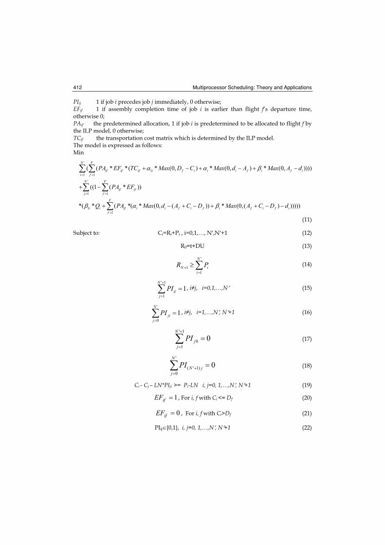
Multiprocessor Scheduling: Theory and Applications 412
PIij 1 if job i precedes job j immediately, 0 otherwise; EFif 1 if assembly completion time of job i is earlier than flight f’s departure time, otherwise 0; PAif the predetermined allocation, 1 if job i is predetermined to be allocated to flight f by the ILP model, 0 otherwise; TCif the transportation cost matrix which is determined by the ILP model. The model is expressed as follows: Min
'
1
1 1
'
1 1
1
1
( ( * *( * (0, ) * (0, ) * (0, ))))
((1 ( * ))
*( * ( *( * (0, ( )) * (0, ( ) )))))
N F
if if if i f i i i f i f ii f
N F
if ifj f
F
i i if i i f i f i f i f if
PA EF TC Max D C Max d A Max A d
PA EF
Q PA Max d A C D Max A C D d
(11)
Subject to: Ci=Ri+Pi , i=0,1,…, N ,N +1 (12)
R0=t+DU (13)
'
1
1
N
Ni
iR P (14)
' 1
1
1N
ijjPI , i j, i=0,1,…,N (15)
'
0
1N
jijPI , i j, i=1,…,N , N +1 (16)
' 1
0
1
0N
jjPI (17)
'
( ' 1)
0
0N
N jjPI (18)
Ci - Cj – LN*PIji >= Pi-LN i, j=0, 1,…,N , N +1 (19)
1ifEF , For i, f with Ci <= Df (20)
0ifEF , For i, f with Ci>Df (21)
PIij {0,1}, i, j=0, 1,…,N , N +1 (22)

Synchronized scheduling of manufacturing and 3PL transportation 413
The decision variables are Ri, PIij, EFif. The objective function includes the two early and two late penalties for the orders. Early penalties are incurred when assembly of the order is completed earlier than its transportation departure time. The late penalties are the special flight transportation cost when orders miss their predetermined flight. Since the assembly scheduling model considers synchronization with transportation, early and late penalty for assembly together with final delivery early and late penalties are taken into account in this model. The first term in the objective function is the cost of early penalties of the orders when they can catch its pre-determined flight. The early penalties consist of earliness cost before transportation, predetermined flight transportation cost, final delivery earliness/tardiness costs. The second term in the objective function is the late penalties of the orders when they miss their predetermined flights. The late penalties consist of the commercial flight transportation cost, the final delivery earliness/tardiness costs. Note that two dummy jobs are created in order to facilitate the representation of the immediate precedence of the jobs. They are the first and the last job which has zero quantity. Constraint (12) represents the relationship among the release time, completion time and processing time of each order. Constraint (13) sets the release time of the first job, R0, to the assembly resume time, which is the sum of delay start time t and the delay duration DU.Constraint (14) sets the release time of the last job, RN’+1, larger or equal to the total processing time of all the jobs. These two constraints denote that there might be inserted idle time between the release times of each two adjacent jobs. Constraint (15) and (17) ensure that all the jobs should have a precedence job except the first job. Constraint (16) and (18) ensures that all the jobs should have a successive job except the last job. Constraint (19) represents the completion time relationship between any two jobs. Constraint (20) and (21) indicate that when a job’s completion time is earlier than a flight departure time, it can catch the flight. Constraint (22) indicates that PIij is 0-1 integer variable.
4.2 NP-completeness proof
To prove the assembly scheduling problem is NP-hard, it is reduced to a single machine scheduling problem with distinct due windows and job dependent earliness/tardiness penalty weights. The reduced problem is then proved to be NP-hard. Thus, the assembly scheduling problem investigated in this chapter is also NP-hard. In the following, the equivalence is established between the reduced problem and the problem studied by Wan & Yen (2002), which is NP-hard. The reduced problem: For the present discussion, the air transportation cost and time is ignored, as well as the final delivery earliness penalties. This is equivalent to say that these parameters take value zero. Therefore, the problem basically becomes a scheduling problem with distinct due-windows and job dependent earliness/tardiness penalty weights for each job. The due-window has a length equal to the difference between the final customer delivery time and transportation departure time. Distinct due-windows: There is waiting cost if an order completed earlier than its assembly due date. As there is no earliness cost for final delivery, only tardiness cost is taken into account if the order is delivered later than the final due-date. Also, it is assumed that the air transportation cost and time are ignored. Therefore, the assembly of orders completed between assembly due-date and final due-date lead to no penalty. It is obvious that the number of flights corresponds to the number of due-dates for assembly. Thus, the assembly

Multiprocessor Scheduling: Theory and Applications 414
due-date is distinct. In addition, the final due-date of each order is distinct. Hence the reduced problem is a distinct due windows scheduling problem. Job dependent earliness penalty: If assembly of a job is completed earlier than its due date, there is a waiting penalty, which depends on the product of the early time and the quantity of the job. Job dependent tardiness penalty: As assumed that if an order is delivered later than its final due date, a late delivery penalty, which is the product of lateness time length and the order quantity, is incurred. Wan & Yen (2002) show that the single machine scheduling problem with distinct due windows to minimize total weighted earliness and tardiness is NP-hard. As the reduced assembly scheduling problem is equivalent to the problem studied by Wan & Yen (2002), the prior problem is NP-hard. Therefore, the assembly scheduling problem studied in this chapter is NP-hard.
4.3 Schedule Repair Heuristics
In many production situations, it is not desirable to reschedule all the non-delayed jobs along with the delayed jobs. Instead, the required changes should be performed in such a way that the entire system is affected as little as possible (Roslöf, et al. 2001). This process is termed schedule repair in this chapter. To repair an unfinished schedule which has delayed orders, its valid parts (or the remaining unaffected schedule) should be re-used as far as possible, and only the parts touched by the disturbance are adjusted (Szelke & Markus 1997). At the beginning of assembly, the schedule obtained using BSSH is executed. Suppose the delay is caused by machine breakdown starting from time t and the assembly resumes after time length DU. Jobs that are to be released between t and t+DU in original schedule are only influenced by the disturbance. In line with the concept of schedule repair, the schedule after time t+DU is valid part and should be kept unchanged. The schedule of the influenced jobs between time t and t+DU should be adjusted. The schedule generated using BSSH methodology will have idle times between job groups, during which the assembly does not work at its full capacity. The idle time can be utilized to process the delayed jobs. Therefore, a heuristic to repair the disturbed schedule is proposed is this section. The main motive is to insert the disturbed job into the idle time spans so that the assembly utilization is improved at the advantage of minimizing the delay penalties for the jobs. If still some jobs cannot be inserted into the idle time span, they are appended after the last job of the final schedule. Figure 2 illustrates this idea in detail.
Figure 2. Illustration of schedule repair heuristic

Synchronized scheduling of manufacturing and 3PL transportation 415
In Figure 2, the x axial denotes time. The blocks denote the scheduled jobs. During time t to t+DU, the jobs predetermined to be processed are denoted using shaded blocks. The delayed jobs are to be inserted into the idle times among the job groups in the BSSH schedule as denoted by the arc in the figure using the following heuristic. The schedule repair heuristic (SRH): 1. Sequence the jobs scheduled between t and t+DU by Longest-Processing Time (LPT)
first rule.2. Insert disturbed jobs into the idle time spans between order groups. Suppose there are
Nd disturbed jobs and are sequenced by LPT rule. Let the BSSH schedule has S idle time spans from time t+DU till the end of the planning period. The detailed steps are:
2.1. i=1, j=12.2. If Length[span(i)]>ProcessingTime[job(j)], insert job j into span i. Else, go to 2.5. 2.3. Length[span(i)]= Length[span(i)]- ProcessingTime[job(j)]. 2.4. j=j+1. If j> Nd, go to 2.7. Else, go to 2.2.
2.5. i=i+1. If S, go to 2.2. Else, go to 2.6.
2.6. Append the remaining Nd -j jobs after the last job of the BSSH schedule. 2.7. Stop. By computational experiments, it is shown that SRH can achieve good results. For detailed content, it can be referred to Li et al. (2006).
5. Conclusion and Further Research
In this chapter, the formulation of synchronized scheduling problem of production and transportation is presented. The solution methodology is to decompose the overall problem into two sub-problems, i.e., the transportation allocation problem and machine scheduling problem. The 3PL transportation allocation problem is formulated using an integer programming model. It is shown that the problem is solvable in polynomial time. Furthermore, the formulations for single machine with and without random delay are presented. The methods to solve these two problems are summarized. Further research can address the assembly sub-problem with parallel machines or sequential machines, etc.
6. References
Chen, Z.L. and Vairaktarakis, G.L., 2005. Integrated Scheduling of Production and Distribution Operations. Management Science, 51(4), 614-628.
Garcia, J.M., Lozano, S. and Canca, D., 2004. Coordinated scheduling of production and delivery from multiple plants. Robotics and Computer-Integrated Manufacturing, 20(3), 191-198.
Li, K.P., Ganesan, V.K and Sivakumar, A.I., 2005. Synchronized scheduling of Assembly and Multi-Destination Air Transportation in Consumer Electronics Supply Chain.
International Journal of Production Research 43(13), 2671-2685.
Li, K.P., Ganesan, V.K. and Sivakumar, A.I., 2006. Scheduling of Single Stage Assembly with Air Transportation in A Consumer Electronics Supply Chain. Computers & Industrial Engineering, 51, 264-278.

Multiprocessor Scheduling: Theory and Applications 416
Panwalkar, S.S., Smith, M.L., and Seidmann, A., 1982, Common due-date assignment to minimize total penalty for the one machine scheduling problem. Operations Research, 30, 391-399.
Roslöf, J., Harjunkoski, I., Björkqvist, J, Karlsson, S. & Westerlund, T. (2001). An MILP-based reordering algorithm for complex industrial scheduling and rescheduling. Computers & Chemical Engineering, 25(4-6), 821-828.
Szelke, E. & Markus G. (1997). A learning reactive scheduler using CBR/L. Computers in Industry, 33, 31-46.
Wan, G.H. & Yen, B.M.P.C. (2002). Tabu search for single machine scheduling with distinct due windows and weighted earliness/tardiness penalties. European Journal of Operational Research, 142(2), 271-281.
Winston, W.L. (1994). Operations research: applications and algorithms (3rd edition). (Duxbury, California).

23
Scheduling for Dedicated Machine Constraint
Arthur Shr1, Peter P. Chen1 and Alan Liu2
1Department of Computer Science, Louisiana State University, 2Department of Electrical Engineering, National Chung Cheng University
1U.S.A., 2Taiwan, R.O.C.
1. Introduction
We have proposed the heuristic Load Balancing (LB) scheduling (Shr et al., 2006a) (Shr et al., 2006b) (Shr et al., 2006c) and Multiagent Scheduling System (MSS) (Shr, et al. 2006d) approaches to provide solutions to the issue of dedicated photolithography machine constraint. The dedicated photolithography machine constraint, which is caused by the natural bias of the photolithography machine, is a new challenge in the semiconductor manufacturing systems. Natural bias will impact the alignment of patterns between different layers. This is especially true for smaller dimension IC for high technology products. A study considered different production control policies for semiconductor manufacturing, including a “machine dedication policy” in their simulation, has reported that the scheduling policy with machine dedication had the worst performance of photolithography process (Akcalt et al., 2001). The machine dedication policy reflects the constraint we are discussing here. In our previous work, along with providing the LB scheduling or MSS approaches to the dedicated machine constraint, we have also presented a novel model––the Resource Schedule and Execution Matrix (RSEM) framework. This knowledge representation and manipulation method can be used to tackle the dedicated machine constraint. A simulation system has also been implemented in these researches and we have applied our proposed scheduling approaches to compare with the Least Slack (LS) time approach in the simulation system (Kumar & Kumar, 2001). The reason for choosing the LS scheduling approach was that this approach was the most suitable method for solving the types of problems caused by natural bias at the time of our survey. The LS scheduling approach has been developed in the research of Fluctuation Smoothing Policy for Mean Cycle Time (FSMCT) (Kumar & Kumar, 2001), in which the FSMCT scheduling policy is for the re-entrant production lines. The entire class of the LS scheduling policies has been proven stable in a deterministic setting (Kumar, 1994) (Lu & Kumar, 1991). The LS approach sets the highest priority to a wafer lot whose slack time is the smallest in the queue buffer of one machine. When the machine becomes idle, it selects the highest priority wafer lot in the queue buffer to service next. However, the simulation result has shown that the performances of both our proposed LB and MSS approaches were better than the LS method. Although the simulations were simplified, they have reflected the real situation we have met in the factory.

Multiprocessor Scheduling: Theory and Applications 418
Extending the previous simulations, we introduce two different types of simulation for the dedicated machine constraint in this paper. One is to show that our proposed LB scheduling approach is still better than the LS approach under the different capacity and service demand of the wafer lots. The case of setting with different photolithography machines represents the different capacity of the semiconductor factory, while the case of setting with different photolithography layers represents the different products’ demand for the semiconductor factory. The other simulation is to show the situation of the thrashing phenomenon, i.e., the load unbalancing among the photolithography machines during the process when we apply the LS approach. We have also learned that the load unbalancing is consistent with different photolithography machines. The rest of the paper is organized as follows: Section 2 describes the motivation of this research including the description of dedicated machine constraint, the load balancing issue, and related research. In Section 3, we present the construction procedure and algorithms of the RSEM framework to illustrate the proposed approach for dedicated machine constraint. The proposed LB scheduling approach is presented along with an example of the semiconductor factory in Section 4. Section 5 shows the simulation results and we conclude the work in Section 6.
2. Motivation
2.1 Dedicated Machine Constraint
Dedicated machine constraint forces wafer lots passing through each photolithography stage to be processed on the same machine. The purpose of the limitation is to prevent the impact of natural bias and to keep a good yield of the IC product. Fig. 1. describes the dedicated machine constraint. When material enters the photolithography stage with dedicated machine constraint, the wafer lots dedicated to machine X need to wait for it, even if machine Y is idle. By contrast, when wafer lots enter into non-photolithography stages without any machine constraints, they can be scheduled to any machine, A, B, or C.
Non-Photolithography Stages
Machine AMachine
BMachine
CMachine
XMachine
YMachine
Z
Busy
Photolithography Stages
With dedicated machine Constraint
idle
Wafer lots
Without dedicated machine Constraint
Wafer lots
Figure 1. Dedicated machine constraint
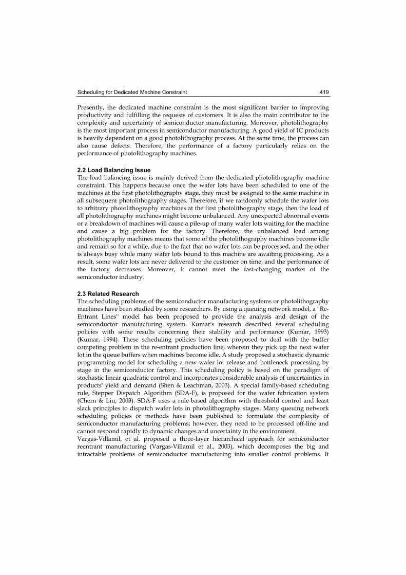
Scheduling for Dedicated Machine Constraint 419
Presently, the dedicated machine constraint is the most significant barrier to improving productivity and fulfilling the requests of customers. It is also the main contributor to the complexity and uncertainty of semiconductor manufacturing. Moreover, photolithography is the most important process in semiconductor manufacturing. A good yield of IC products is heavily dependent on a good photolithography process. At the same time, the process can also cause defects. Therefore, the performance of a factory particularly relies on the performance of photolithography machines.
2.2 Load Balancing Issue
The load balancing issue is mainly derived from the dedicated photolithography machine constraint. This happens because once the wafer lots have been scheduled to one of the machines at the first photolithography stage, they must be assigned to the same machine in all subsequent photolithography stages. Therefore, if we randomly schedule the wafer lots to arbitrary photolithography machines at the first photolithography stage, then the load of all photolithography machines might become unbalanced. Any unexpected abnormal events or a breakdown of machines will cause a pile-up of many wafer lots waiting for the machine and cause a big problem for the factory. Therefore, the unbalanced load among photolithography machines means that some of the photolithography machines become idle and remain so for a while, due to the fact that no wafer lots can be processed, and the other is always busy while many wafer lots bound to this machine are awaiting processing. As a result, some wafer lots are never delivered to the customer on time, and the performance of the factory decreases. Moreover, it cannot meet the fast-changing market of the semiconductor industry.
2.3 Related Research
The scheduling problems of the semiconductor manufacturing systems or photolithography machines have been studied by some researchers. By using a queuing network model, a ''Re-Entrant Lines'' model has been proposed to provide the analysis and design of the semiconductor manufacturing system. Kumar's research described several scheduling policies with some results concerning their stability and performance (Kumar, 1993) (Kumar, 1994). These scheduling policies have been proposed to deal with the buffer competing problem in the re-entrant production line, wherein they pick up the next wafer lot in the queue buffers when machines become idle. A study proposed a stochastic dynamic programming model for scheduling a new wafer lot release and bottleneck processing by stage in the semiconductor factory. This scheduling policy is based on the paradigm of stochastic linear quadratic control and incorporates considerable analysis of uncertainties in products' yield and demand (Shen & Leachman, 2003). A special family-based scheduling rule, Stepper Dispatch Algorithm (SDA-F), is proposed for the wafer fabrication system (Chern & Liu, 2003). SDA-F uses a rule-based algorithm with threshold control and least slack principles to dispatch wafer lots in photolithography stages. Many queuing network scheduling policies or methods have been published to formulate the complexity of semiconductor manufacturing problems; however, they need to be processed off-line and cannot respond rapidly to dynamic changes and uncertainty in the environment. Vargas-Villamil, et al. proposed a three-layer hierarchical approach for semiconductor reentrant manufacturing (Vargas-Villamil et al., 2003), which decomposes the big and intractable problems of semiconductor manufacturing into smaller control problems. It

Multiprocessor Scheduling: Theory and Applications 420
reduces the effort and frequency of the control decisions. The scheduling problems of the photolithography machines have been studied by some researchers. Their proposed scheduling methods make an effort to improve the performance of the photolithography machines. Two approaches were reported to use simulations to model the photolithography process. One of them proposed a Neural Network approach to develop an intelligent scheduling method according to a qualifying matrix and lot scheduling criteria to improve the performance of the photolithography machines (Mönch et al., 2001). The other approach decides the wafer lots assignment of the photolithography machines at the time when the wafer lots are released to the manufacturing system in order to improve the load-balancing problem (Arisha & Young, 2004). These researches have emphasized that photolithography process scheduling issues are the most important and critical challenge of the semiconductor manufacturing system. However, it might be difficult to have the proper training data to build a Neural Network scheduling system. It is also inefficient to manually adjust lot scheduling criteria or lot assignment to fit the fast-changing market of semiconductor manufacturing. Moreover, their proposed scheduling methods did not concern the dedicated machine constraint.
3. Resource Schedule and Execution Matrix (RSEM) Framework
In this section, the procedure and algorithm associated with the Resource Schedule and Execution Matrix (RSEM) framework are presented. The RSEM framework construction process consists of three modules including the Task Generation, Resource Calculation, and Resource Allocation modules. The first module, Task Generation, models the tasks for the scheduling system and it is represented in a two-dimensional task matrix. One dimension is reserved for the tasks, t1, t2,…, tn; the other represents the periodical time events (or steps) s1, s2, …,sm. Each task has a sequential Process Pattern to represent the resources it needs to go from the raw material to a product during the process sequence and we put the process pattern in an array. We define each type of resource as rk, k =1 to o. For example, the process pattern, r1, r2, …, ro,means that a particular task needs the resources in the sequence of r1 first and r2 following that until ro is gained. Therefore, the matrix looks as follows:
s1 s2 . . sq . . . sj . sm
t1 r1 r2 r3 .. .. .. ... .. .. .. ..
t2 r3 r4 .. .. .. .. .. .. .. ..
. r1 r3 .. .. .. ..
ti r3 r4 .. .. rk ..
. . .
tn .. .. .. .. .. ..

Scheduling for Dedicated Machine Constraint 421
The symbol rk in the task matrix entry [ti, sj] represents that task ti needs the resource rk at the time sj. If ti starts to be processed at sq, and the total number of steps needed for ti is p, we will fill its process pattern into the matrix from [ti, sq]… to [ti, sq+p-1] with rk, k =1 to o. All the tasks, t1…tn, follow the illustration above to form a task matrix in the Task Generationmodule. To represent dedicated machine constraint in the matrix for this research, the symbol rkx, a replacement of rk, represents that ti has been dedicated to a particular instance xof a resource type rk at sj. One more symbol wk represents the wait situation when the rk
cannot allocate to ti at sj. The situation can be that rk is assigned to other higher priority tasks or it is breakdown. This symbol will be used in the Resource Allocation module. The Resource Calculation module summarizes the value of each dimension as the factors for the scheduling rule of the Resource Allocation module. For example, by counting the task pattern of the row ti in the task matrix, we can determine how many steps ti processed after it finished the whole process. We can also realize how many wait steps ti has had by counting wk from the starting step to the current step in that row of the task matrix. Furthermore, if we count the symbol rkx at the column sj, we can know how many tasks will need the machine mx of resource rk at sj.We need to generate the task matrix, obtain all the factors for the scheduling rules, and build up the scheduling rules before starting the execution of the Resource Allocation module. The module schedules the tasks to the suitable resource according to the factors and predefined rules. To represent the situation of waiting for rk ; i.e. when the resource of rk is not available for ti at sj, then we will not only insert the symbol wk in the pattern of ti , but will also need to shift one step for the process pattern following ti in the matrix. Therefore, we can obtain the updated factor for the number of tasks waiting for rk at sj by simply counting wk at the column sj. We can also obtain the factor for the number of wait steps ti has by counting wk,
1≤k≤o by the row ti in the matrix. Our proposed approach can provide two kinds of functions. One is that, to define the factors and resource allocation rules according to expert knowledge, we can quickly determine the allocation of resources at each step by the factors summarized from the task matrix. The other is that we can predict the bottleneck or critical situation quickly by executing proper steps forward. This can also evaluate the predefined rules to obtain better scheduling rules for the system at the same time. Moreover, by using different predefined rules and factors, the RSEM framework could apply to different scheduling issues or constraints of semiconductor manufacturing.
3.1 Procedure for Constructing the RSEM framework
To better understand our proposed scheduling process, the flowchart of the RSEM framework construction process is shown in Fig. 2. The process of using the RSEM framework starts from the Task Generation module, and it will copy the predefined task patterns of tasks into the matrix. Entering the Resource Calculation module, the factors for the tasks and resources will be brought out at the current step. This module will update these factors again at each scheduling step. The execution of the scheduling process is in the Resource Allocation module. When we have scheduled for all the tasks for the current step, we will return to check for new tasks and repeat the whole process again by following the flowchart. We will exit the scheduling process when we reach the final step of the last task if there is still no new task appended to the matrix. After that, the scheduling process will restart immediately when the new tasks arrives in the system.

Multiprocessor Scheduling: Theory and Applications 422
Figure 2. Flowchart of the RSEM framework construction process
3.2 Algorithms Associated to the RSEM framework
To make the construction process of the proposed RSEM framework more concrete, three algorithms for the Task Generation (Algorithm-1), Resource Calculation (Algorithm-2), and Resource Allocation (Algorithm-3) modules are depicted as follows. In Algorithm-1, the procedure appends tasks to the task matrix by copying the task patterns of the tasks in the matrix. It will start from the start step ss and go to the end step se of each task. The ss will not start before the current step sc and the se should not end beyond the maximum step m of the matrix in the system. The task matrix will be passed to and manipulated at the other two algorithms.
Algorithm-1 Task_Generation{// sc ss se m, where m is the max step in system, and // sc is current step.
for i = 1 to n doCopy task pattern of ti into matrix from its starting step ss, to its ending step se
next }

Scheduling for Dedicated Machine Constraint 423
Algorithm-2 Resource_Calculation{
//Factor for tasks, function: Total_Step(ti)//To count total steps of tasks n: total tasks, m: max step in system.
for i = 1 to n dofor j = 1 to m do;
if (matrix[ti,sj] is not empty) thenTotal_Step(ti)= Total_Step(ti) + 1; /*Count total steps*/
end if next
next //Factor for tasks, function: Wait_Step(ti)//To count total wait steps of tasks, sc: current step.
for i = 1 to n dofor j = 1 to sc do;
if (matrix[ti,sj] = wk) thenWait_Step(ti)= Wait_Step(ti) + 1; /*Count wait steps*/
end if next
next //Factor for resource, function: Resource_Demand(rk)//To count total tasks which are need of the resource rk
//o: total resource.
for k = 1 to o dofor i = 1 to n do
if (matrix[ti,sc] = rk) thenResource_Demand(rk)= Resource_Demand(rk) + 1;
end if next
next //Factor for Resource, function: Queue_Buffer(rk)//To count total tasks which are waiting for of the resource rk
for k = 1 to o dofor i = 1 to n do
if (matrix[ti,sc] = wk) thenQueue_Buffer(rk)=+1;
end if next
next
//Factor for ...
…. // factor Load, Utilization, and so on.
}
We will have four factors ready for scheduling after the Resource Calculation process described in Algorithm-2, namely, Total_Step(ti) and Wait_Step(ti) for the tasks, and Resource_Demand(rk) and Queue_Buffer(rk) for the resources.

Multiprocessor Scheduling: Theory and Applications 424
We obtain these factors by simply counting the occurrences of the desired symbols like rk or wk, along the specific task ti dimension or the current step sc of the task matrix. We can also include other factors in this module depending on different applications, e.g., the factors of the load of a particular photolithography machine and the remaining photolithography stages of the tasks in the example of Section 3. The procedure of Algorithm-3 executes the scheduling process for the tasks and resources. The first part of the scheduling process allocates all the available resources to optimize the performance or production goals of the manufacturing system, but it must satisfy all the constraints. The scheduling rule of our proposed Load Balancing approach is one of the examples. After the process for resource allocation, the second part of the scheduling process is to insert a wait step and shift a step for all the tasks which are not assigned to a machine. A wait symbol wk represents the state of waiting for machine type k, and a wkx is waiting for dedicated machine number x, mx, of machine type k.
Algorithm-3 Resource_Allocation{
//Scheduling; o: total resource, sc:current step.
for k = 1 to o doAssign tasks to rk, according to predefined rules
e.g., the Load Balancing scheduling (LB), Multiagent Scheduling System (MSS) or
Least Slack time scheduling (LS) rules
next
//Execution; shift process pattern of the tasks,
//which do not be scheduled at current step;
//x: the machine number.
for i = 1 to n doif (ti will not take the resource at this step) then
insert wk to wait for rk; /* without dedicated constraint */
orinsert wxk to wait for mx of rk; /*dedicated constraint */
end if next
}
4. Load Balancing Scheduling Method
In this section, we apply the proposed Load Balancing (LB) scheduling method to the dedicated machine constraint of the photolithography machine in semiconductor manufacturing. The LB method uses the RSEM framework as a tool to represent the temporal relationship between the wafer lots and machines during each scheduling step.
4.1 Task Generation
After obtaining the process flow for customer product from the database of semiconductor manufacturing, we can use a simple program to transform the process flow into the matrix representation. There exist thousands of wafer lots and hundreds of process steps in a

Scheduling for Dedicated Machine Constraint 425
typical factory. We start by transforming the process pattern of wafer lots into a task matrix.
We let r2 represent the photolithography machine and rk (k ≠ 2) represent non-photolithography machines. The symbol r2x in the matrix entry [i,j] represents the wafer lot ti
needing the photolithography machine mx at the time sj with dedicated machine constraint,
while rk (k ≠ 2) in [i,j] represents the wafer lot ti needing the machine type k at sj without dedicated machine constraint. There is no assigned machine number for the photolithography machine before the wafer lot has passed the first photolithography stage. Suppose that the required resource pattern of t1 is as follows: r1r3r2r4r5r6r7r2r4r5r6r7r8r9r1r3r2r4r5r6r7r3r2r8r9…and starts the process in the factory at s1. We will fill its pattern into the matrix from [t1,s1] to [t1,sn], which indicates that t1 needs the resource r1 at the first step, resource r3 at the second step, and so on. The photolithography process, r2, in this process pattern has not been dedicated to any machine and the total number of steps for t1 is n. The task t2 in the task matrix has the same process pattern as t1 but starts at s3;meanwhile, ti in the matrix starts at s8. It requires the same type of resource r2, the photolithography machine, but the machine is different from the machine t2 needed at s10;i.e., t2 needs the machine m1, while ti has not been dedicated to any machine yet. Two tasks, t2 and ti, might compete for the same resource r4 at s11 if r4 is not enough for them at s11. The following matrix depicts the patterns of these tasks.
s1 s2 s3 s4 s5 s6 s7 s8 s9 s10 s11 s12 s13 .. .. s20 s21 s22 s23 s24 s25 .. .. sj .. sm
t1 r1 r3 r2 r4 r5 r6 r7 r2 r4 r5 r6 r7 r8 .. .. r6 r7 r3 r2 r8 r9 .. .. .t2 r1 r3 r2 r4 r5 r6 r7 r21 r4 r5 r6 .. .. r4 r5 r6 r7 r3 r2 r8 r9 .. ..
..
ti r1 r3 r2 r4 r6 r5 .. .. .. .. .. .. .. .. .. .. rk ..
4.2 Resource Calculation
The definitions and formulae of these factors for the LB scheduling method in the Resource Calculation module are as follows:
W: wafer lots in process, Wp : wafer lots dedicated to the photolithography machine, p, P: numbers of photolithography machines, R(ti): remaining photolithography layers for the wafer lot ti,K: types of machine (resource), ss: start step, sc: current step, se: end step.
Required resources: • How many wafer lots will need the k type machine x at sj?
PxrsttsrRRWt
xkjiij
xk
i
≤≤==∈
1,}][|{),( , (1)
Count steps: • How many wait steps did ti have before sj?
KkwstttWaitStepc
s
s
sjkjiii ≤≤==
=1},],[|{)(
(2)

Multiprocessor Scheduling: Theory and Applications 426
• How many steps will ti have?
≠==
e
s
s
sjjiii nullstttSteps }],[|{)(
(3)
• The load factor, Lp, of the photolithography machine p.
∈×=
pi Wtiip tRtL )}({ (4)
Lp is defined as the wafer lots that are limited to machine p multiplied by the remaining layers of photolithography stages these wafer lots have. Lp is a relative parameter, representing the load of the machine and wafer lots limited to one machine compared to other machines. A larger Lp means that more required service from wafer lots is limited to this machine. The LB scheduling method uses these factors to schedule the wafer lot to a suitable machine at the first photolithography stage, which is the only photolithography stage without the dedicated constraint.
4.3 Resource Allocation
The process flow of the Resource Allocation module for the example is described in this section. Suppose we are currently at sj, and the LB scheduling method will start from the photolithography machine. We check to determine if there is any wafer lot that is waiting for the photolithography machines at the first photolithography stage. The LB method will assign the p with the smallest Lp for them, one by one. After that, these wafer lots will be dedicated to a photolithography machine. For each p, the LB method will select one wafer lot of Wp that has the largest WaitStep(ti) for it. The load factor, Lp, will be updated after these two processes. The other wafer lots dedicated to each p, which cannot be allocated to the p at current step sj, will insert a w2 in their pattern. For example, at s10, ti has been assigned to p; therefore, ti+1 will have a w2 inserted into s10, and then all the following required resources of ti+1 will shift one step. All other types of machines will have the same process without need to be concerned with the dedicated machine constraint. Therefore, we assigned the wafer lot that has the largest WaitStep(ti), then the second largest, and so on for each machine rk. Similarly, the LB method will insert a wk for the wafer lots which will not be assigned to machines rk at this current step. Therefore, WaitStep(ti) represents the delay status of ti.
s9 s10 s11 s12 s13 s14 .. .. sj .. sm
.. .. ..
ti .. r2p r4 r6 r5 r7 .. ..
ti+1 .. w2 r2p r4 r6 r5 .. .. .. ..
.. ↑ → → → →

Scheduling for Dedicated Machine Constraint 427
4.4 Discussion
Realistically, it is not difficult to approximate the real machine process time for different steps using one or several steps together with a smaller time scale step. We can also use the RSEM framework to represent complex tasks and allocate resources by simple matrix calculation. This reduces much of the computation time for the complex problem. Another issue is that the machines in the factory have a capacity limitation due to the capital investment, which is the resource constraint. The way to make the most profit for the investment mostly depends on optimal resource allocation techniques. However, most scheduling policies or methods can provide neither the exact allocation in an acceptable time, nor a robust and systematic resource allocation strategy. We use the RSEM framework to represent complex tasks and allocate resources by simple matrix calculation. This reduces much of the computation time for the complex problem.
5. Simulation
We have done two types of simulations using both the Least Slack (LS) time scheduling and our LB approach. The LS policy has been developed in the research, Fluctuation Smoothing Policy for Mean Cycle Time (FSMCT) (Kumar & Kumar, 2001). The FSMCT scheduling policy is for re-entrant production lines. The LS scheduling policy sets the highest priority to a wafer lot whose slack time is the smallest in the queue buffer of one machine. When the machine becomes idle, it will select the highest priority wafer lot in the queue buffer to service next. The entire class of LS policies has been proven stable in a deterministic setting (Kumar, 1994) (Lu & Kumar, 1991), but without the dedicated machine constraint. To simplify the simulation to easily represent the scheduling approaches, we have made the following assumptions: (1) each wafer lot has the same process steps and quantity, and (2) there is an unlimited capacity for non-photolithography machines
5.1 Simulation Results
We implemented a simulation program in Java and ran the simulations on NetBeans IDE 5 (http://www.netbeans.org/). To represent the different capacity and required resource demand situation for a semiconductor factory, we take account of different photolithography machines and wafer lots with different photolithography layers in the simulation program. Our simulation was set with 6, 10, 13, and 15 photolithography machines, and 11 to 15 photolithography layers. There are 1000 wafer lots in the simulation. The wafer arrival rate between two wafer lots is a Poisson distribution. We also set up the probability of breakdown with 1% for each photolithography machine at each step in the simulation. The duration of each breakdown event may be 1 to 4 steps and their individual probability is based on a Uniform distribution. Fig. 3(a) illustrated the average Mean Time Between Failures (MTBF) and Mean Time Between Repairs (MTBR) of different photolithography machines, i.e. in the case of 6 machines the average of MTBF and MTBR is 101.03 and 2.97 steps, respectively. While the average MTBF and MTBR of different photolithography layers are shown in Fig. 3(b), in the case of 15 layers the average of MTBF and MTBR is 102.56 and 3.30 steps, respectively.

Multiprocessor Scheduling: Theory and Applications 428
Machine Breakdown -- Different Machines
100.19
101.57
101.89101.03
2.97 2.98 2.99 3.00
0
25
50
75
100
125
6 10 13 15Machine
Step
0
1
2
3
4
5
Step
MTBF MTBR
(a)
Machine Breakdown -- Different Layers
103.23 102.56101.09
100.1198.85
3.03
3.00 2.96 2.96 2.97
0
25
50
75
100
125
11 12 13 14 15Layer
Step
0
1
2
3
4
5
Step
MTBF
MTBR
(b)
Figure 3. MTBF and MTBR of machine breakdown

Scheduling for Dedicated Machine Constraint 429
In the task patterns, the symbol r represents the non-photolithography stage; and r2 the photolithography stage. The basic task pattern for 11 layers is: “rrrrr2rrrrrrrrrrrrrrr2r2r2r2r2r2rrrrrrrrrrrrrrrr2r2r2r2rrrrrrrrrrrrrrrrrr2r2r2rrrrrrrr2r2rrrrrrr2r2rrrrr2r2rrrrr2r2rrrrr2r2rrrrr2r2rrrrr2r2rrrr”. Then the task pattern for each added layer after 11 layers is: “r2rrrr”. Therefore, the task pattern for 12 layers is: “rrrrr2rrrrrrrrrrrrrrr2r2r2r2r2r2rrrrrrrrrrrrrrrr2r2r2r2rrrrrrrrrrrrrrrrrr2r2r2rrrrrrrr2r2rrrrrrr2r2rrrrr2r2rrrrr2r2rrrrr2r2rrrrr2r2rrrrr2r2rrrrr2r2rrrr”,…, and the task pattern for 15 layers is: “rrrrr2rrrrrrrrrrrrrrr2r2r2r2r2r2rrrrrrrrrrrrrrrr2r2r2r2rrrrrrrrrrrrrrrrrr2r2r2rrrrrrrr2r2rrrrrrr2r2rrrrr2r2rrrrr2r2rrrrr2r2rrrrr2r2rrrrr2r2rrrrr2r2rrrrr2r2rrrrr2r2rrrrr2r2rrrr”. The task matrix for 15 layers looks as follows:
s1 ……………………………………………………………………………… sm
t1 rrrrr2rrrrrrrrrrrrrrr2r2r2r2r2r2rrrrrrrrrrrrrrrr2r2r2r2rrrrr........r2r2rrrrt2 rrrrr2rrrrrrrrrrrrrrr2r2r2r2r2r2rrrrrrrrrrrrrrrr2r2r2r2rrrrr........r2r2rrrr.. :
ti rrrrr2rrrrrrrrrrrrrrr2r2r2r2r2r2rrrrrrrrrrrrrrrr2r2r2r2rrrrr..........
t1000 :
Task Matrix (15 photolithography layers)
Both LB and LS approaches were applied to the same task matrix during each simulation generated by the Task Generation module described in Section 3. The result of simulation, as described in detail in the following subsections, shows the advantage of the LB approach over the LS approach under different numbers of machines by the average of the different photolithography layers, and under different numbers of layers by the average of the different photolithography machines. Different Photolithography Machines: By comparing the mean of cycle time, in the case of 6 machines, the LS method has 164.49 (LS-LB) steps more than the LB approach. That is 7.12% ((LS-LB)/LS) more in the simulation. The different steps from machines 10 to 15 incrementally rise from 175.54 to 184.16 steps and the percentages of the difference rises from 14.92% to 28.83%. The simulation result of different photolithography machines indicates that the more photolithography machines, the better the LB approach performs than the LS method does. The simulation result is shown in Fig. 4(a). Different Photolithography Layers: On the other hand, the simulation result of different layers (11 to 15 layers) indicates that there is no significant difference with different photolithography layers. The outperformance in percentage of the LB approach is between the minimum, 16.71%, to the maximum, 19.72%. Such a simulation result is shown in Fig. 4(b).

Multiprocessor Scheduling: Theory and Applications 430
Simulation Result -- Different Machines
184.16172.05
175.54164.49
7.12%
14.92%21.73%
28.83%
0
50
100
150
200
6 10 13 15Machine
Step(LS-LB)
0%
10%
20%
30%
40%
%((LS-LB)/LS)
Diff Step %
(a). Different Photolithography Machines
Simulation Result -- Different Layers
187.11201.56
171.33
164.63
145.68
16.71%19.72%
19.27%
17.73% 17.32%
0
50
100
150
200
250
11 12 13 14 15Layer
Step(LS-LB)
0%
10%
20%
30%
40%
50%
%((LS-LB)/LS)
Diff Step
%
(b) Different Photolithography Layers
Figure 4. Simulation results

Scheduling for Dedicated Machine Constraint 431
5.2 Thrashing and Load Unbalancing
After applying the LS approach to the above simulations and counting the required resource (Equation (1): RR(rkx, sj) of Section 4.2, k=2, x=6, 10, 13, 15) for the photolithography machines at each step, we can observe that the load balancing status in terms of the difference between maximum and minimum counts of the required resource for the machines becomes larger and unstable, i.e., the thrashing phenomenon takes place in the simulations. The simulation is set with 6, 10, 13, and 15 photolithography machines and 15 photolithography layers. In the simulation, the Max-Min and Standard Deviation of wafer lots in machine buffers set with 6, 10, 13, and 15 machines are shown in the graphs in Fig. 5 ((a), (b), (c), and (d)), respectively. The simulation results also reveal that the fewer machines the system has, the worse the situation of an unbalanced load would be to the system. On the other hand, while applying the LB method, the load balancing status is stable and consistent with different machines, and it is always less then 2.5 at each execution step.
6. Conclusion
We presented the Resource Schedule and Execution Matrix (RSEM) framework–a novel representation and manipulation method for the tasks in this paper. The RSEM framework is used as a tool to analyze the issue of dedicated machine constraint and develop solutions. The simulation also showed that the proposed LB scheduling approach was better than the LS method in various situations. Although the simulations are simplified, they reflect the real situation we have met in the factory. The advantage of the proposed RSEM framework is that we can easily apply various policies to the scheduling system by simple calculation on a two-dimensional matrix. The matrix architecture is easy for practicing other semiconductor manufacturing problems in the area with a similar constraint. We also want to apply other scheduling rules to the Resource Allocation module in the RSEM framework. Our intended future work is to develop a knowledge-based scheduling system for the Resource Allocation module or to model it as distributed constraint satisfaction scheduling project.

Multiprocessor Scheduling: Theory and Applications 432
Max-Min & STD of Machine Buffers - LS Method with 6 Machines
0
10
20
30
40
50
60
Step
=0
Step
=200
Step
=400
Step
=600
Step
=800
Step
=1000
Step
=1200
Step
=1400
Step
=1600
Step
=1800
Step
=2000
Step
=2200
Step
=2400
Step
=2600
Step
=2800
Step
=3000
Step
=3200
Step
=3400
Step
=3600
Step
=3800
Step
=4000
Step
=4200
Step=44
00
Step
=4600
Step=48
00
Step
=5000
Step
=5200
Step
=5400
Step
=5600
Step
=5800
STD
Max-Min
Max STD = 19.93
Max-Min & STD of Machine Buffers - LB Approach with 6 Machines
0
10
20
30
40
50
60
Step
=0
Step
=180
Step
=360
Step
=540
Step=72
0
Step
=900
Step
=1080
Step=12
60
Step
=1440
Step
=1620
Step
=1800
Step
=1980
Step=21
60
Step
=2340
Step
=2520
Step
=2700
Step=28
80
Step
=3060
Step
=3240
Step
=3420
Step
=3600
Step=37
80
Step
=3960
Step
=4140
Step
=4320
Step=45
00
Step
=4680
Step
=4860
Step
=5040
Step
=5220
STD
Max-Min
Max STD = 2.19
Figure 5(a). Thrashing phenomenon—6 machines

Scheduling for Dedicated Machine Constraint 433
Max-Min & STD of Machine Buffers - LS Method with 10 Machines
0
10
20
30
40
50
60
Step
=0
Step
=130
Step=26
0
Step
=390
Step
=520
Step
=650
Step
=780
Step=91
0
Step
=1040
Step
=1170
Step
=1300
Step=14
30
Step
=1560
Step
=1690
Step
=1820
Step=19
50
Step
=2080
Step
=2210
Step
=2340
Step=24
70
Step
=2600
Step
=2730
Step
=2860
Step=29
90
Step
=3120
Step
=3250
Step
=3380
Step
=3510
Step=36
40
Step
=3770
STD
Max-Min
Max STD = 13.99
Max-Min & STD of Machine Buffers - LB Approach with 10 Machines
0
10
20
30
40
50
60
Step
=0
Step
=110
Step
=220
Step
=330
Step
=440
Step
=550
Step
=660
Step
=770
Step
=880
Step
=990
Step
=1100
Step
=1210
Step
=1320
Step
=1430
Step
=1540
Step
=1650
Step
=1760
Step
=1870
Step
=1980
Step
=2090
Step
=2200
Step
=2310
Step
=2420
Step
=2530
Step
=2640
Step
=2750
Step
=2860
Step
=2970
Step
=3080
Step
=3190
STD
Max-Min
Max STD = 1.96
Figure 5(b). Thrashing phenomenon—10 machines

Multiprocessor Scheduling: Theory and Applications 434
Max-Min & STD of Machine Buffers - LS Method with 13 Machines
0
10
20
30
40
50
60
Step=0
Step
=100
Step
=200
Step
=300
Step=40
0
Step=50
0
Step
=600
Step=70
0
Step
=800
Step=90
0
Step
=1000
Step=11
00
Step
=1200
Step=13
00
Step
=1400
Step=15
00
Step
=1600
Step=17
00
Step=18
00
Step
=1900
Step
=2000
Step
=2100
Step=22
00
Step
=2300
Step=24
00
Step
=2500
Step=26
00
Step=27
00
Step=28
00
STD
Max-Min
Max STD = 11.03
Max-Min &STD of Machine Buffers - LB Approach with 13 Machines
0
10
20
30
40
50
60
Step
=0
Step
=90
Step
=180
Step
=270
Step
=360
Step
=450
Step
=540
Step
=630
Step
=720
Step
=810
Step
=900
Step
=990
Step
=1080
Step
=1170
Step
=1260
Step
=1350
Step
=1440
Step
=1530
Step
=1620
Step
=1710
Step=18
00
Step=18
90
Step=19
80
Step=20
70
Step
=2160
Step
=2250
Step
=2340
Step
=2430
STD
Max-Min
Max STD = 1.85
Figure 5(c). Thrashing phenomenon—13 machines

Scheduling for Dedicated Machine Constraint 435
Min-Max & STD of Machine Buffers - LS Method with 15 Machines
0
10
20
30
40
50
60
Step=0
Step=11
0
Step=22
0
Step=33
0
Step=44
0
Step=55
0
Step=66
0
Step=77
0
Step=88
0
Step=99
0
Step=11
00
Step=12
10
Step=13
20
Step=14
30
Step=15
40
Step=16
50
Step=17
60
Step=18
70
Step=19
80
Step
=2090
Step=22
00
Step
=2310
Step
=2420
Step=25
30
Step
=2640
Step=27
50
Step
=2860
Step
=2970
STD
Max-Min
Max STD = 10.09
Min-Max & STD of Machine Buffers - LB Approach with 15 Machines
0
10
20
30
40
50
60
Step=0
Step=90
Step=18
0
Step=27
0
Step=36
0
Step=45
0
Step=54
0
Step=63
0
Step=72
0
Step=81
0
Step=90
0
Step=99
0
Step=10
80
Step=11
70
Step=12
60
Step=13
50
Step=14
40
Step=15
30
Step=16
20
Step
=1710
Step
=1800
Step=18
90
Step=19
80
Step=20
70
Step=21
60
Step=22
50
Step=23
40
Step=24
30
STD
Max-Min
Max STD = 1.77
Figure 5(d). Thrashing phenomenon—15 machines
7. Acknowledgments
This research was partially supported by the U.S. National Science Foundation grant No. IIS-0326387 and U.S. AFOSR grant: FA9550-05-1-0454. This research was also supported in part by the Ministry of Economic Affairs under the grant 95-EC-17-A-02-S1-029 and the

Multiprocessor Scheduling: Theory and Applications 436
National Science Council under the grants 95-2752-E-008-002-PAE and 95-2221-E-194-009. A. Shr is grateful to Ms. Erin Sinclair for English proofreading.
8. References
Akcalt. E., Nemoto. K. & Uzsoy. R. (2001) Cycle-time improvements for photolithography process in semiconductor manufacturing. IEEE Transactions on Semiconductor Manufacturing, 14, 48-56.
Arisha. A. & Young. P. (2004) Intelligent Simulation-based Lot Scheduling of Photolithography Toolsets in a Wafer Fabrication Facility. 2004 Winter Simulation Conference, Washington, D.C., USA, 1935-1942.
Chern. C. & Liu. Y. (2003) Family-Based Scheduling Rules of a Sequence-Dependent Wafer Fabrication System. IEEE Transactions on Semiconductor Manufacturing, 16, 15-25.
Kumar. P. R. (1993) Re-entrant Lines. Queuing Systems: Theory and Applications, Special Issue on Queuing Networks, 13, 87-110.
Kumar. P. R. (1994) Scheduling Manufacturing Systems of Re-Entrant Lines. Stochastic Modeling and Analysis of Manufacturing Systems, 13, D.D. Yao (ed.), Springer-Verlag, New York, 87-110.
Kumar. S. & Kumar. P. R. (2001) Queuing Network Models in the Design and Analysis of Semiconductor Wafer Fabs. IEEE Transactions on Robotics and Automation, 17, 548-561.
Lu. S. H. & Kumar. P. R. (1991) Distributed Scheduling Based on Due Dates and Buffer Priorities. IEEE Transactions on Automatic Control, 36, 1406-1416.
Mönch. L., Prause. M., & Schmalfuss. V. (2001) Simulation-Based Solution of Load-Balancing Problems in the Photolithography Area of a Semiconductor Wafer Fabrication Facility. 2001 Winter Simulation Conference, Virginia, USA, 1170-1177.
Shen. Y. & Leachman. R. C. (2003) Stochastic Wafer Fabrication Scheduling. IEEE Transactions on Semiconductor Manufacturing, 1, 2-14.
Shr. A. M. D., Liu. A., & Chen. P. P. (2006a) A Load Balancing Scheduling Approach for Dedicated Machine Constraint. Proceedings of the 8th International Conference on Enterprise Information Systems ICEIS 2006, pp. 170-175, Paphos, Cyprus.
Shr. A. M. D., Liu. A., & Chen. P. P. (2006b) A Heuristic Load Balancing Scheduling Approach for Dedicated Machine Constraint. Proceedings of the 19th International Conference on Industrial, Engineering & Other Applications of Applied Intelligent Systems (IEA/AIE'06), Lecture Notes in Artificial Intelligence (LNAI) 4031, M. Ali and R. Dapoigny (Eds), Springer-Verlag, Berlin Heidelberg, pp. 750-759.
Shr. A. M. D., Liu. A., & Chen. P. P. (2006c) A Load Balancing Method for Dedicated Photolithography Machine Constraint. Proceedings of the 7th IFIP International Conference on Information Technology for Balanced Automation Systems in Manufacturing and Services (BASYS'06), IFIP International Federation for Information Processing, Vol. 220, Information Technology for Balanced Automation Systems, Shen, W. Ed., (Boston Springer), pp. 339-348.
Shr. A. M. D., Liu. A., & Chen. P. P. (2006d) Load Balancing among Photolithography Machines in Semiconductor Manufacturing. Proceedings of the 3rd IEEE International Conference on Intelligent Systems (IEEE IS'06), pp. 320-325, London, England.
Vargas-Villamil. F. D., Rivera. D. E., & Kempf. K. G. (2003) A Hierarchical Approach to Production Control of Reentrant Semiconductor Manufacturing Lines. IEEE Transactions on Control Systems Technology, 11, 578-587.

![[J22]on Parallelizing the Multiprocessor Scheduling Problem](https://static.fdocuments.us/doc/165x107/577d2c881a28ab4e1eac7be1/j22on-parallelizing-the-multiprocessor-scheduling-problem.jpg)


