Branch and Bound Algorithm for Multiprocessor Scheduling

Branch and Bound Algorithm for Multiprocessor

Scheduling

M Mostafizur Rahman

2009

Masters Thesis

Computer Science-

Applied Artificial

Intelligence

Nr. E3713D

DEGREE PROJECT

in Computer Science Program

International Masters Programme in Computer

Science - Applied Artificial Intelligence

Reg number

E3713D

Extent

15 ECTS (10 weeks)

Name of student

Md. Mostafizur Rahman

Year-Month-Day

2009-02-21

Supervisor

Dr. Pascal Rebreyend

Examiner

Prof. Dr. Mark Dougherty

Department of Computer Engineering

Title

Branch and Bound Algorithm for Multiprocessor Scheduling

Key Words Multiprocessor scheduling problems, Branch and Bound, Lower Bound, Upper Bound, Task

Graph Scheduling, Critical Path.

Abstract:

The multiprocessor task graph scheduling problem has been extensively studied as

academic optimization problem which occurs in optimizing the execution time of parallel

algorithm with parallel computer. The problem is already being known as one of the NP-

hard problems. There are many good approaches made with many optimizing algorithm

to find out the optimum solution for this problem with less computational time. One of

them is branch and bound algorithm.

In this paper, we propose a branch and bound algorithm for the multiprocessor scheduling

problem. We investigate the algorithm by comparing two different lower bounds with

their computational costs and the size of the pruned tree.

Several experiments are made with small set of problems and results are compared in

different sections.

ACKNOWLEDGEMENTS

First of all I would like to thanks to Almighty Allah, who has given me the strength to

successfully reach to the end of this program.

I would like to express my sincere gratitude to my Supervisor, Pascal Rebreyend, for

providing his valuable time and suggestion for the completion of this project. His strong

hold & vast knowledge of Algorithm and heuristic helped me a lot to come to the

successful end of the project, without him, the research could not have been completed.

I give my deepest thanks to Prof. Mark Dougherty for teaching us the course Algorithms

and complexity and my sincere thanks to the entire faculty member in Computer

Engineering department for their support in various ways.

To my mother Ruby and father Moazzam as well as siblings for their support during my

studies. Most important, I would like to thank my lovely wife Asma for her love and

strong mental support during my study. Finally, my deepest love and care goes to my one

and only little M Ahnaf Rahman, who make me laugh more than anyone I know.

Table of Contents:

1.0 Introduction ……………………………………………………………………..2

2.0 Aim and Objectives……………………………………………………………...4

2.1 Scope of the project……………………………………………………..4

2.2 Work plan………………………………………………………………..4

2.3 Limitations ……………………………………………………………....4

3.0 Problem Description……………………………………………………………..5

3.1 Definition for multiprocessor task scheduling problem…………………5

4.0 Literature Review and branch and bound algorithm……………………………8

4.1 Application of BnB…………………………………………………….10

5.0 Developing the Branch and Bound Algorithm for the MTSP…………………..12

5.1 Branching Scheme ……………………………………………………..12

5.2 Bounding Scheme ………………………………………………………13

5.3 Branch and Bound Algorithm for the MTSP……………………………18

5.4 Example of the application of BnB algorithm in a DAG………………..20

6.0 Experimental Results and Analysis:……………………………………………...23

6.1 Discussion ……………………………………………………………… 34

7.0 Conclusion and future work:…………………………………………………….38

M Mostafizur Rahman Degree Project 2009

E3713D

Högskolan Dalarna TeL: 023 77 8000

Röda Vägen 3, 781 88 Fax: 023 77 8050

Borlänge www.du.se

2

1.0 Introduction

Now a days the computing system is becoming more complex and people are running

after to find out solution for efficient way for allocating the resource of the computer

system. One of the interesting and major problems is the task scheduling in the

multiprocessor environment. The utilization of parallel processing systems these days, in

a vast variety of applications, is the result of numerous breakthroughs over the last two

decades. The development of parallel and distributed systems has lead to there use in

several applications including information processing, fluid flow, weather modeling,

database systems, real-time high-speed simulation of dynamical systems, and image

processing. The data for these applications can be distributed evenly on the processors of

parallel and distributed systems, and thus maximum benefits from these systems can be

obtained by employing efficient task partitioning and scheduling strategies [1]. The

multiprocessor task schedule problem is NP-hard. Although it is possible for formulate

and solve the problem using heuristics, the feasible solution space quickly becomes

intractable for larger problem instance.

When the structure of the parallel program such as number of task, execution time of

tasks, dependency constraints, communication cost, and the number of processors are

known beforehand, a schedule is determined statically at compile time. Except for a few

special cases, no polynomial-time algorithm that finds the schedule with a minimum

length exists For that reason, many heuristic algorithms have been developed to obtain

suboptimal solutions to various scheduling problems, some of them are Branch and

Bound Ant Colony Optimization, Genetic Algorithm, Tabu Search, Simulated Annealing,

Graph Theoretic and Computational Geometry Approaches. But very few research has

been made with Branch and Bound algorithm.

In this project I have considered the Branch and Bound algorithm to solve the

multiprocessor task graph scheduling. Branch-and-bound (BnB) techniques can be used

to reduce the amount of search needed to find the optimal solution. BnB is based on a

common-sense principle: do not keep trying a path that we already know is worse than

the best answer. One of the first articles on branch-and-bound was (Lawler and Wood,


E3713D


Röda Vägen 3, 781 88 Fax: 023 77 8050

Borlänge www.du.se

3

1966). A more readable introduction is in (Winston, 1984). A simple algorithm describes

the method (mostly from (Winston, 1984)):

The critical problem that is found for solving that Multi Processor Scheduling is the delay

in communication of the data from one task to other task defining a precedence

relationship for the set of task, being predecessor and successor. Our concern is assumed

in the problem of scheduling dependencies tasks onto multiprocessor system with

processors connected in an arbitrary way, while explicitly accounting for the time

required to transfer data between the tasks allocated to different processors. The delay in

communication therefore occurs whenever two pair of tasks (predecessor, successor) is

assigned to different processors.

Each processor can perform single task at a time and all the necessary information

(number of tasks, number of processor, task cost, dependency, and communication time)

are assumed to be known.

The problem is defined as a directed acyclic graph (DAG). Where the vertices represent

the program modules, but a (directed) arc indicates a direct 1-way communication

between a predecessor and successor pair of modules.

The main part of this project is to develop a branch and bound algorithm to find out an

optimum solution form the search tree, with less computational time and creating

minimum numbers of node.


E3713D


Röda Vägen 3, 781 88 Fax: 023 77 8050

Borlänge www.du.se

4

2.0 Aim and Objective:

The idea behind this thesis is to develop a branch and bound algorithm for searching for

the optimal solution for the Multi Processor Scheduling problem and define a branching

scheme for eliminating unnecessary branching.

2.1 Scope of the project:

• The project is focusing about the following issue

• Design of a good scheme to enumerate all solutions

• Design a Branch and Bound algorithm to search the optimum solution form the

search tree.

• Comparison of different Lower Bound.

2.2. Work Plan:

2.3 Limitations of the Project:

As the project span was 10 weeks, it was really hard to find out sufficient time for

designing a good and efficient algorithm for the problem.

One of the biggest problems that I faced is lack of reference for this specific scheduling

problem. There are many research has been made with Branch and Bound algorithm but

not a single one is made for this specific problem that we have addressed in this paper.

Week 1 Week 2 Week 2 Week 3 Week 4 Week 5 Week 6 Week 7 Week 8 Week 9 Week 10

Litera

ture

Revie

w

Algorithm Design and Coding with C

programming Language

Lowe r Bound

test

Result analysis & report

writing


E3713D


Röda Vägen 3, 781 88 Fax: 023 77 8050

Borlänge www.du.se

5

3.0 Problem Description:

The multiprocessor task scheduling problem considered in this paper is based on the

deterministic model, which is the execution time of tasks and the data communication

time between tasks that are assigned; and, the directed acyclic task graph (DAG) that

represents the precedence relations of the tasks of a parallel processing system well

known as the NP-complete problem.

Considering the following problem; given a set of identical processors, we face a number

of independent requests for processing tasks. Each request is characterized by a multi-

processor task with (a) its required processing period, (b) required processor for the

whole period (c) the corresponding time/cost of processing the task.

3.1 Definition for multiprocessor task scheduling problem:

Multiprocessor task scheduling problem (MTSP), for this project can be defined as:

(homogeneous) multiprocessor system be a set of P = {p1,…..,pm} is a set of m identical

processor, m >1 connected by a complete interconnection network, where all links are

identical.[pas1] Each processor has its own memory and can execute only one task at a

time. During the execution processor will communicate exclusively by message passing

through the interconnection network. There is a set of n tasks (ti) is to be scheduled on a set

of m identical processors. Where schedule could be seen as the sequence and time in which

the tasks (ti) are executed with (i = 0….n). Each task is associated with a cost that

represents the execution time of the task and also a number of precedence constrains. It’s

more convenient to use a weighted acyclic task digraph to represent the problem.[pas 2] .

A task graph is a weighted DAG with G = (T, E), where the set of nodes (corresponding

to processors) and E is a set of communication edges. W is the set of node weights, and C

is the set of edge weights. Given a task graph TG and a number of processors P, whereas

MTSP is to distribute tasks (ti) in TG onto m computational processors, which is fully

connected in order for the precedence constraints to be satisfied and the execution time of

the task graph minimized. There is no preemption or duplication of task in this case. [2-

3].


E3713D


Röda Vägen 3, 781 88 Fax: 023 77 8050

Borlänge www.du.se

6

The vertices represent the set T = { t1……… tn} of tasks and each arc represents the

precedence relation between two tasks. An arc ( t1,tn ) ∈ E represents the fact that at the

end of its execution, ti1 sends a message whose contents are required by ti2 to start

execution. In this case, ti1 is said to be an immediate predecessor of ti2 , and ti2 itself is

said to be an immediate successor of ti1 . We suppose that t1 is the only task without any

immediate predecessor. A path is a sequence of nodes < ti1,…..,tik > , 1 < k < n such that

til is an immediate predecessor of ti l+1, 1 < l < k. A task ti1 is a predecessor of another

task tik if there is a path < ti1,…..,tik > in D. To every task ti, there is an associated value

representing its duration, and we assume that these values are known before the execution

of the program. [2-3].

P1 P2t1

t2

t3

t4

t5

Cost:

t1=t

2=t

3=2

t4=5

t5=1

c(ti,t

j) = communication time needed between t

i and t

j = 2

Micro Processor System

D

comp=comma=comb = 1


E3713D


Röda Vägen 3, 781 88 Fax: 023 77 8050

Borlänge www.du.se

7

It is assumed that the duration of all the communications is also known at compile-time.

Thus, to every arc (ti1, ti2) ∈ E there is an associated cost representing the transfer time of

the message sent by ti1 to ti2 . If both message source and destination are scheduled to the

same processor, then the cost associated to this arc becomes null. [2-3].

There are some attributes for the parallel machine, “comp”,“comma”,and ”comb”. “comp” is

the performance factor of the machine, means if a task (a node of the graph) costs x, than

it's execution time will be comp *x. “comma” and “commb” are the communication's

parameters. “commb” represents the time to start a communication between two nodes

and “comma” represents the time (without start-up time) to communicate a data, e.g. If

nodes a must send h data to node b, node b can not start before the end of execution of a

plus comma *x+ commb time's units, if the tasks a and b are scheduled to different

processor.

A schedule can be represented by S = {s1,……..,sn} where sj = { ti1,…..,tinj} , where sj is the

sto of the nj set of the tasks scheduled to pj . For each task til ∈ sj, l represents its

execution rank in pj under the schedule s.

The execution time yielded by a schedule is known as “make span”. Our objective was to

develop a Branch and Bound algorithm to search an optimum solutions (having minimum

“make span”) form the search space, by making less branches and creating minimum

numbers of nodes, and also to detect if one sub-tree can be discarded in the search

because it’s worst then other.


E3713D


Röda Vägen 3, 781 88 Fax: 023 77 8050

Borlänge www.du.se

8

4.0 Literature Review:

Branch and bound (BnB) is a general algorithm for finding optimal solutions of various

optimization problems, especially in discrete and combinatorial optimization. It consists

of a systematic enumeration of all candidate solutions, where large subsets of fruitless

candidates are discarded en masse, by using upper and lower estimated bounds of the

quantity being optimized. The method was first proposed by A. H. Land and A. G. Doig

in 1960 for linear programming. [wikipedia].

General description

For definiteness, we assume that the goal is to find the minimum value of a function f(x)

(e.g., the cost of manufacturing a certain product), where x ranges over some set S of

admissible or candidate solutions (the search space or feasible region). Note that one can

find the maximum value of f(x) by finding the minimum of g(x) = − f(x).

A branch-and-bound procedure requires two tools. The first one is a splitting procedure

that, given a set S of candidates, returns two or more smaller sets whose

union covers S. Note that the minimum of f(x) over S is , where each

vi is the minimum of f(x) within Si. This step is called branching, since its recursive

application defines a tree structure (the search tree) whose nodes are the subsets of S.

Another tool is a procedure that computes upper and lower bounds for the minimum

value of f(x) within a given subset S. This step is called bounding.

The key idea of the BB algorithm is: if the lower bound for some tree node (set of

candidates) A is greater than the upper bound for some other node B, then A may be

safely discarded from the search. This step is called pruning, and is usually implemented

by maintaining a global variable m (shared among all nodes of the tree) that records the

minimum upper bound seen among all subregions examined so far. Any node whose

lower bound is greater than m can be discarded.


E3713D


Röda Vägen 3, 781 88 Fax: 023 77 8050

Borlänge www.du.se

9

The recursion stops when the current candidate set S is reduced to a single element; or

also when the upper bound for set S matches the lower bound. Either way, any element of

S will be a minimum of the function within S.

Effective subdivision

The efficiency of the method depends strongly on the node-splitting procedure and on the

upper and lower bound estimators. All other things being equal, it is best to choose a

splitting method that provides non-overlapping subsets.

Ideally the procedure stops when all nodes of the search tree are either pruned or solved.

At that point, all non-pruned subregions will have their upper and lower bounds equal to

the global minimum of the function. In practice the procedure is often terminated after a

given time; at that point, the minimum lower bound and the minimum upper bound,

among all non-pruned sections, define a range of values that contains the global

minimum. Alternatively, within an overriding time constraint, the algorithm may be

terminated when some error criterion, such as (max - min)/(min + max), falls below a

specified value.

The efficiency of the method depends critically on the effectiveness of the branching and

bounding algorithms used; bad choices could lead to repeated branching, without any

pruning, until the sub-regions become very small. In that case the method would be

reduced to an exhaustive enumeration of the domain, which is often impractically large.

There is no universal bounding algorithm that works for all problems, and there is little

hope that one will ever be found; therefore the general paradigm needs to be implemented

separately for each application, with branching and bounding algorithms that are

specially designed for it.

Branch and bound methods may be classified according to the bounding methods and

according to the ways of creating/inspecting the search tree nodes.


E3713D


Röda Vägen 3, 781 88 Fax: 023 77 8050

Borlänge www.du.se

10

The branch-and-bound design strategy is very similar to backtracking in that a state space

tree is used to solve a problem. The differences are that the branch-and-bound method (1)

does not limit us to any particular way of traversing the tree and (2) is used only for

optimization problems.

This method naturally lends itself for parallel and distributed implementations, see, e.g.,

the traveling salesman problem.

It may also be a base of various heuristics. For example, one may wish to stop branching

when the gap between the upper and lower bounds becomes smaller than a certain

threshold. This is used when the solution is "good enough for practical purposes" and can

greatly reduce the computations required. This type of solution is particularly applicable

when the cost function used is noisy or is the result of statistical estimates and so is not

known precisely but rather only known to lie within a range of values with a specific

probability. An example of its application here is in biology when performing cladistic

analysis to evaluate evolutionary relationships between organisms, where the data sets are

often impractically large without heuristics.

For this reason, branch-and-bound techniques are often used in game tree search

algorithms, most notably through the use of alpha-beta pruning.

4.1 Application of BnB :

Branch and Bound algorithm is applied in many NP-Hard problems like:

* Traveling salesman problem (TSP) (is a problem in combinatorial optimization

studied in operations research and theoretical computer science. Given a list of cities and

their pairwise distances, the task is to find a shortest possible tour that visits each city

exactly once.) [See ref: 4]


E3713D


Röda Vägen 3, 781 88 Fax: 023 77 8050

Borlänge www.du.se

11

* Knapsack problem (is a problem in combinatorial optimization. It derives its name

from the following maximization problem of the best choice of essentials that can fit into

one bag to be carried on a trip.) [See ref: 5]

* Integer programming (If the unknown variables are all required to be integers, then

the problem is called an integer programming (IP) or integer linear programming (ILP)

problem. In contrast to linear programming, which can be solved efficiently in the worst

case, integer programming problems are in many practical situations (those with

bounded variables) NP-hard.) [See ref: 5]

* Nonlinear programming (nonlinear programming (NLP) is the process of solving a

system of equalities and inequalities, collectively termed constraints, over a set of

unknown real variables, along with an objective function to be maximized or minimized,

where some of the constraints or the objective function are nonlinear.)

* Quadratic assignment problem (QAP) (is one of fundamental combinatorial

optimization problems in the branch of optimization or operations research in

mathematics, from the category of the facilities location problems.

* Maximum satisfiability problem (MAX-SAT) (asks for the maximum number of

clauses which can be satisfied by any assignment. It is an NP-hard problem, but not NP;

and it is an APX-Complete problem, but not PTAS.)

* Nearest neighbor search (NNS) (also known as proximity search, similarity search or

closest point search, is an optimization problem for finding closest points in metric

spaces. The problem is: given a set S of points in a metric space M and a query point q

∈ M, find the closest point in S to q. In many cases, M is taken to be d-dimensional

Euclidean space and distance is measured by Euclidean distance or Manhattan distance.)

There are very few research is done with Branch and Bound to solve scheduling problem.

There are few article found for solving specific problems of multiprocessor scheduling

see [4,5,6], but not a single article found for the specific problem that we are addressing

in this paper.


E3713D


Röda Vägen 3, 781 88 Fax: 023 77 8050

Borlänge www.du.se

12

5.0 Developing the Branch and Bound Algorithm for the MTSP:

In this section, we propose a branch and bound algorithm for searching the optimal

solution for the problem describe in the section 3.1. In this section, we describe the B&B

algorithm developed in this research. For branching, i.e., for selecting a node to generate

branches from, the depth-first rule is used. That is, a node with the most unit-jobs

included in the associated partial schedule is selected for branching. In case of ties, a

node with the lowest lower bound is selected.

When child nodes are generated from a selected parent node, it is checked whether or not

schedules associated with the child nodes are dominated by using dominance properties

that can be obtained from the section 5.1 and 5.2, the lower bound and upper bound given

in Section 5.2 is computed for every child node. Nodes with lower bounds that are greater

than to the upper bound, i.e., the solution value of the current incumbent solution, are

deleted from further consideration (fathomed). In addition with that a global variable

bestUB is maintained (shared among all nodes of the tree) that records the minimum

upper bound seen among all subregions examined so far. Any node whose lower bound is

greater than bestUB can be discarded. The recursion stops when the current candidate set

µ(α) is reduced to a single element; or also when the upper bound of the selected node

matches the lower bound and all the task are scheduled.

5.1 Branching Scheme

Multi Processor Task Scheduling Problem as described in section 3.1, there are Ti,

i=1,…,n tasks to be schedule to P = {p1,…..,pm} is a set of m identical processor by

maintaining the precedence relation between two tasks. Cti is the cost of the task ti.. CC is

the communication cost of an arc; CCij = ( ti,tj ) ∈ E represents the fact that at the end of

its execution, ti1 sends a message whose contents are required by ti2 to start execution. In

this case, ti1 is said to be an immediate predecessor of ti2 , and ti2 itself is said to be an

immediate successor of ti1 .


E3713D


Röda Vägen 3, 781 88 Fax: 023 77 8050

Borlänge www.du.se

13

Creating partial solutions:

Each node α in the search tree is defined by α = (Sα1…….. Sαm ), Tα,, kα . Sαi represents a

sequence of scheduled tasks on the processor i for node α. Tα is the list of all the

unscheduled job in the node α. kα is the list of computational time (end time) of all

scheduled tasks in (Sα1…….. Sαm ). ∂(α) denotes a partial schedule consisted of m sequences

Sαi, i = 1.,,,.m. µ(α) is the set of all the child nodes of the node α, which are also known as

the open nodes means the nodes not yet been expended. µ(α) can be obtained by a

scheme discuss next.

Branching out from a node α is carried out creating a new node and coping all the

information form the node α. Scheduling is done by taking a t form the list of Tα for

which all the predecessor are already been scheduled, and appending it to the tail of

sequence Sαi, i = 1.,,,.m. we are repeat this for all the combination of i and j where i∈P

={1...m} and j∈ Tα ={1…n}.

Let the newly created node be node β and the related sequence be Sβi,. Tβ = Tα/{j} (Tβ will

be the new list of unscheduled task after scheduling the task j). Which shows that the β is

the partial schedule with one more task scheduled then the node α. [1-2]. We will add all

the newly created children nodes from the parent node α in the µ(α) as a open node.

After creating all the possible children from the parent node, the will be immediately

removed from the list of open nodes for not considering further expansion.

A node α will be selected again depending upon the branching rule for next expansion, in

this case the node which has lowest bound value will be selected first. The details of the

bounding of the search space is discuss next.


E3713D


Röda Vägen 3, 781 88 Fax: 023 77 8050

Borlänge www.du.se

14

5.2 Bounding Scheme:

For the branch and bound algorithm we have used two heuristics value for every created

node one is upper bound and another is lower bound. LBα and , UBα, known as

upperbound and lowebound are the two heuristic value for the partial solution ∂(α).

Upper Bound:

Upper bounds are tested by calculating using simply greedy heuristics shortest Job First

SJF and also lowest starting time first (LSTF).

SJF: was calculated using the scheduling scheme shortest job first the algorithm of the

upper bound is given below:

Input: node β , Number of task N, Number of processor M, task cost and communication

costs.

Output: Make span.


E3713D


Röda Vägen 3, 781 88 Fax: 023 77 8050

Borlänge www.du.se

15

UB with Greedy SJF: 1. while (number of unscheduled task >0)

a. for each processor Pi ∈ P do the followings

i. select a task that has a minimum cost and all the predecessors are already

scheduled

ii. get the start time of the task to be scheduled to Pi

1. start time = MAX [end time of the predecessors + communication cost]

iii. Schedule the task to Pi in the sequence of Sβ

iv. Update kβ

b. End While

2. compute make span

3. return make span as the upper bound of the node

UB With Greedy LSTF: 4. while (number of unscheduled task >0)

i. select a task which all the predecessors are already scheduled

ii. get the CPU Pi for which the task has the lowest starting time

iii. Schedule the task to Pi in the sequence of Sβ

iv. Update kβ

b. End While

5. compute make span

6. return make span as the upper bound of the node

Lower Bound:

For the Branch and Bound algorithm we have tested two Lower Bounds to establish the minimum

growth rate of the algorithm and compare the results that are shown in the section…. Several

studies are devoted to the parallel machine scheduling problem with heads and tails. We

first review the lower bounds. Carlier [6] presents several lower bounds based on

machine load. Carlier and Pinson [7] introduce the concept of pseudo-preemptive

schedule and Gharbi and Haouari [8] derive several lower bounds from the lower bound

proposed byWebster [9] for the parallel machine problem with resource availability constraints,

but there is no such proved lower bound for the specific problem that we are addressing in this

paper.

A simple lower bound LB1 of every newly created node is calculated in the following function:

+ = ∑

m

CT β

β LB partial schedule time

βTC is cost of all unscheduled tasks in the node β

m is the number of processor where m> 1


E3713D


Röda Vägen 3, 781 88 Fax: 023 77 8050

Borlänge www.du.se

16

For LB2 we have chosen the critical path. It was developed in the 1950s by the US

Navy when trying to better organize the building of submarines and later, especially,

when building nuclear submarines. Today, it is commonly used with all forms of

scheduling problems.

t1=2

t2=2 t

3=2

t4=5

t5=1

D

0

1

6

8

1

Longest path length

from the exit node

Cost of the node

Critical path from t0

to t5

Critical Path Example


E3713D


Röda Vägen 3, 781 88 Fax: 023 77 8050

Borlänge www.du.se

17

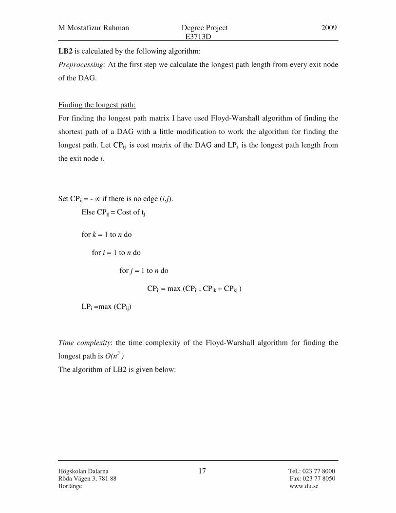
LB2 is calculated by the following algorithm:

Preprocessing: At the first step we calculate the longest path length from every exit node

of the DAG.

Finding the longest path:

For finding the longest path matrix I have used Floyd-Warshall algorithm of finding the

shortest path of a DAG with a little modification to work the algorithm for finding the

longest path. Let CPij is cost matrix of the DAG and LPi is the longest path length from

the exit node i.

Set CPij = - ∞ if there is no edge (i,j).

Else CPij = Cost of tj

for k = 1 to n do

for i = 1 to n do

for j = 1 to n do

CPij = max (CPij , CPik + CPkj )

LPi =max (CPij)

Time complexity: the time complexity of the Floyd-Warshall algorithm for finding the

longest path is O(n3

)

The algorithm of LB2 is given below:


E3713D


Röda Vägen 3, 781 88 Fax: 023 77 8050

Borlänge www.du.se

18

LB2:

For each unscheduled task ti do the followings

If all the predecessor of task ti is already been scheduled (i = 1,…number of unscheduled task )

Compute the minimum starting sti of the task ti

cPathi = sti + cost of ti + LPi

End IF

End of For

LB2 = max (cPathi ) (i = 1,…number of unscheduled task )

If LB2 < the partial make span then

LB2 = + = ∑

m

CT β

β LB partial schedule time [βTC is cost of all unscheduled tasks in the node β

m is the number of processor where m> 1]

END IF

5.3 Branch and Bound Algorithm for MTSP:

In this section we are going to propose a branch and bound algorithm following the

branching and bounding schemes stated in section 5.1 and 5.2.

Some notations:

Cti = Cost of the task ti

CCij = communication cost between the task i, j.

µ(α) = list of all the open nodes, which not yet been expended

T β = List of all unscheduled job in the partial solution node β

jkβ = End time of the task j in the partial solution node β

The Pseudo Code of the algorithm is given in the next page.


E3713D


Röda Vägen 3, 781 88 Fax: 023 77 8050

Borlänge www.du.se

19

BEGIN

Step 1: (Initialization)

1.1. Set Cti = cost of all the tasks for i = 1 to n

1.2. Set CCij = ( ti,tj ) ∈ E for i = 1 to n and for j = 1 to n

1.3. µ(α) = {}

1.4. Create a root node α of the search tree Set α = (Sα1…….. Sαm )= { }

1.5. Set Tα= ti, i = 1….n, kαi = -1, i = 1….n

1.6. add the root node α as open list in the first place of µ(α)

1.7. go to step 2.1

Step 2: (Branching from a node)

2.1. start branching

2.2. for each pair of (j, i) do the followings, where j ∈ Tα , i ∈ P = 1,...m

2.2.1. Create a child node β by copying all the information form

the parent node α.

2.2.2. If all the predecessors of the task j is already been

scheduled Then

2.2.2.1.The new schedule of β, can be obtain by appending

a new task j at the tail of sequence of Sβi .

2.2.2.2.Compute the start time by following the rule of the

communication cost of the task j for the processor i.

2.2.2.3. set the status of the task j, j

kβ = Cj+ start time

2.2.2.4. compute the partial Make Span of the node β

2.2.2.5. compute LB β

2.2.2.6. compute UB β

2.2.2.7. IF UB β < BestUB THEN

2.2.2.7.1. set BestUB = UB β

2.2.2.7.2. delete all the node form µ(α) that has LB

> BestUB

2.2.2.8. END IF

2.2.2.9. IF LB β > UB β THEN

2.2.2.9.1. delete the node β

2.2.2.10. ELSE

2.2.2.10.1. add the node as a open list in µ(α)

2.2 END of FOR

2.3 Select a node β from the open nodes list µ (α) for which the LB is

the minimum among all the nodes in the list.

2.4 Set α = β

2.5 IF LBα,= UBα AND Tα= { } THEN

2.5.3 STOP the algorithm

2.6 ELSE 2.6.3 Go to step 2.2

END


E3713D


Röda Vägen 3, 781 88 Fax: 023 77 8050

Borlänge www.du.se

20

1 2 3 4 5 6 7 8 9 10 11

P2

P1t1

t2

t1

t3

t4

t5

P1 P2t1

t2

t3

t4

t5

Cost:

t1=t

2=t

3=2

t4=5

t5=1

c(ti,t

j) = communication time needed between t

i and t

j = 2

Micro Processor System

D

time

comp=comma=comb = 1

Schedule S :

{{t1, t

2, t

4, t

5},{t

3}}

5.4 Example of the application of BnB algorithm in a DAG:

Figure 2 shows the optimum solution found by the branch and bound algorithm of the

DAG shown above. The detail search iteration is shown next in the figure 3.

Fig2: Optimum Schedule found by the BnB for a DAG


E3713D


Röda Vägen 3, 781 88 Fax: 023 77 8050

Borlänge www.du.se

21

1

23

UB: 13. LB: 7UB: 13. LB: 7

4

UB: 19. LB: 11

5

UB: 21. LB: 11

6

UB: 13. LB: 11

7UB: 19. LB: 11

8

UB: 16. LB: 8

9

UB: 18. LB: 8

10

UB: 16. LB: 11

11UB: 16. LB: 11

12

UB: 15. LB: 9

13UB: 19. LB: 10

20

UB: 12. LB: 11

21 UB: 18. LB: 14

14

UB: 15. LB: 9

15

UB: 15. LB: 10

16

UB: 13. LB: 12

17 UB: 13. LB: 13

18

UB: 12. LB: 11

19 UB: 16. LB: 12

22

UB: 12. LB: 11

23

UB: 11. LB: 11

24 25

UB: 16. LB: 15UB: 16. LB: 15

In the search tree shown in figure 3 we can see that node 1 which is the root node having

partial solution as null { }. At this stage only task 1 is ready to execute, so from that node

the BnB algorithm makes two child nodes one for scheduling the task 1 to processor one

and another for task 1 to processor 2, having upper bound as 13 and lower bound as 7 for

both, and then they are added to the list of open nodes and the root node marked as a

Fig3: Search tree

{}


E3713D


Röda Vägen 3, 781 88 Fax: 023 77 8050

Borlänge www.du.se

22

closed node. As LB (lower bound) of all the nodes in the list of open nodes are equal, the

algorithm selects node number 3 for expending next. As task 1 is scheduled and task 2

and 3 become free to be scheduled to processor 1 or 2. From the node 3 there are four

new child nodes are created for the combination of 2 jobs to 2 processors, having (UB,

LB) as (19,11), (21,11), (13,11), (19,11) and they are added in the list of open list. For

expending next the algorithm selects the node 2 as it has the lowest lower bound among

all the nodes that are in the list of open nodes. This is how it proceeds for further

expansion. When it comes to node number 23 the algorithm found that the upper bound

and lower bound are equal for that partial schedule node, there it stops the algorithm and

prints the upper bound of the node as a found optimum solution. During the creation of

the child nodes when ever the algorithm computes the upper bound and lower bound for a

partial solution node it will check if the lower bound of the node is grater then the upper

bound of the node or not, if it matches then this newly created node is deleted from the

open list. The algorithm maintains a global variable for storing the best known upper

bound. During the creation of a new node the algorithm compare the upper bound of the

node with the best known upper bound and if it is found that the upper bound of the new

node is less then the best known upper bound then it updates the best know upper bound

with the upper bound of the new node, and delete all the nodes that are having lower

bound grater then the best know upper bound. We can see in the figure 3 that the nodes

21, 24 and 25 are deleted from the list of all the open nodes for having lower bound

grater then the best known upper bound.

The searching sequence for the optimum solution for the DAG shown is figure 2 is:

N1 N3 N2 N9 N8 N14 N12 N15 N13 N23


E3713D


Röda Vägen 3, 781 88 Fax: 023 77 8050

Borlänge www.du.se

23

6.0 Experimental Results and Analysis:

The proposed Branch and Bound algorithm was implemented in visual C++ 2008; all the

computational experiments are conducted on a personal computer with Intel 1.6 GHz and

a RAM size of 2 GB in windows vista operating system.

In order to assess the effectiveness of the proposed branch and bound algorithm, we

conduct experiments on some randomly generated task graph DAG. For N ∈ {4, 6,

8,10,15} and M ∈ {2,3,4,5}. Table1 shows the output with the lower bound method one.

Using Lower Bound Method 1 (LB1)

Number

of task

n

Number of

processor

m

Number of

node created

with out

pruning

Number

of node

after

pruning

Number of

Branch made

Average CPU time

in milliseconds

2 19 9 7 5

3 34 10 8 8

4 53 11 9 12

4

5 73 12 10 16

2 55 27 21 10

3 88 28 22 12

4 125 29 23 16

6

5 116 30 24 19

2 1327 662 452 125

3 2089 683 473 203

4 2913 702 492 250

8

5 3706 717 503 359

2 1381 701 313 203

3 1936 718 282 312

4 5073 934 633 608

10

5 6356 822 634 780

2 2424 1230 549 356

3 3398 1260 495 548

4 8903 1639 1256 1067

15

5 11155 1443 1317 1369

From the table above and the following graphs we can see that the number of nodes are

increasing with respect to the number of task.

Table 1


E3713D


Röda Vägen 3, 781 88 Fax: 023 77 8050

Borlänge www.du.se

24

number of Node with LB1 with out pruning

0

2000

4000

6000

8000

10000

12000

4 6 8 10 15

Number of tasks

Nu

mb

ers

of

no

de

P=2

p=3

P=4

p=5

number of Node with LB1 with pruning

0

200

400

600

800

1000

1200

1400

1600

1800

4 6 8 10 15

Number of tasks

Nu

mb

ers

of

no

de

P=2

p=3

P=4

p=5

If we analysis the result with respect to the unnecessary nodes that the algorithm can

prune then we can find that the algorithm is able to cut good numbers of unnecessary

nodes for further expansion where there is no possibility to have the optimum result.


E3713D


Röda Vägen 3, 781 88 Fax: 023 77 8050

Borlänge www.du.se

25

CPU Time Vs Tasks with LB1

0

200

400

600

800

1000

1200

1400

1600

4 6 8 10 15

Number of tasks

CP

U t

ime i

n M

ilis

eco

nd

s

P=2

p=3

P=4

p=5

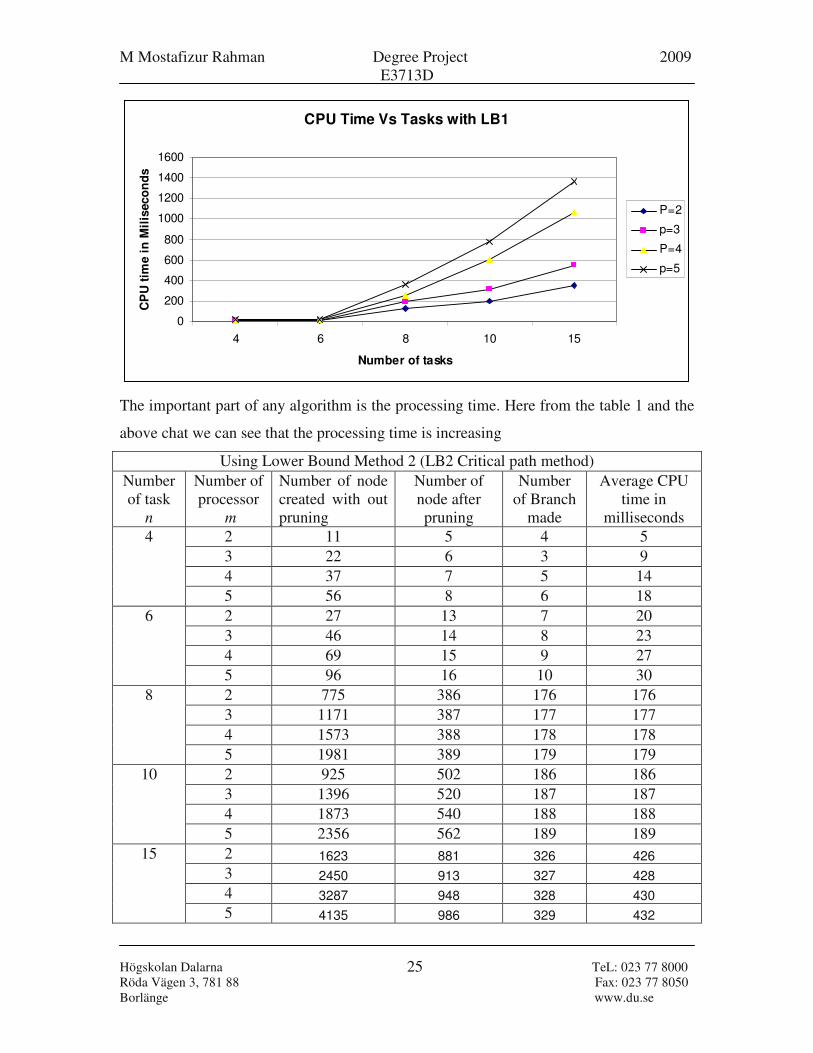
The important part of any algorithm is the processing time. Here from the table 1 and the

above chat we can see that the processing time is increasing

Using Lower Bound Method 2 (LB2 Critical path method)

Number

of task

n

Number of

processor

m

Number of node

created with out

pruning

Number of

node after

pruning

Number

of Branch

made

Average CPU

time in

milliseconds

2 11 5 4 5

3 22 6 3 9

4 37 7 5 14

4

5 56 8 6 18

2 27 13 7 20

3 46 14 8 23

4 69 15 9 27

6

5 96 16 10 30

2 775 386 176 176

3 1171 387 177 177

4 1573 388 178 178

8

5 1981 389 179 179

2 925 502 186 186

3 1396 520 187 187

4 1873 540 188 188

10

5 2356 562 189 189

2 1623 881 326 426

3 2450 913 327 428

4 3287 948 328 430

15

5 4135 986 329 432


E3713D


Röda Vägen 3, 781 88 Fax: 023 77 8050

Borlänge www.du.se

26

Node Number Vs Tasks with LB2 with out pruning

0

500

1000

1500

2000

2500

3000

3500

4000

4500

4 6 8 10 15

Number of tasks

Nu

mb

ers

of

no

de

P=2

p=3

P=4

p=5

Node Number Vs Tasks with LB2 after pruning

0

200

400

600

800

1000

1200

4 6 8 10 15

Number of tasks

Nu

mb

ers

of

no

de

P=2

p=3

P=4

p=5


E3713D


Röda Vägen 3, 781 88 Fax: 023 77 8050

Borlänge www.du.se

27

CPU Time Vs Tasks with LB2

0

50

100

150

200

250

300

350

4 6 8 10 15

Number of tasks

CP

U t

ime i

n M

ilis

eco

nd

s

P=2

p=3

P=4

p=5

Comparison result of LB1 and LB2

Number

of task

n

Number of

processor

m

Node with

LB1

Average

CPU time in

milliseconds

Node with

LB2

Average CPU

time in

milliseconds

2 9 5 5 5

3 10 8 6 9

4 11 12 7 14

4

5 12 16 8 18

2 27 10 13 20

3 28 12 14 23

4 29 16 15 27

6

5 30 19 16 30

2 662 125 386 176

3 683 203 387 177

4 702 250 388 178

8

5 717 359 389 179

2 701 203 502 186

3 718 312 520 187

4 934 608 540 188

10

5 822 780 562 189

2 1230 356 881 426

3 1260 548 913 428

4 1639 1067 948 430

15

5 1443 1369 986 432

Table 3


E3713D


Röda Vägen 3, 781 88 Fax: 023 77 8050

Borlänge www.du.se

28

Table 3 shows the comparison result of lower bound 1 and lower bound 2, there we can

see that LB2 is creating less node then LB1 to find the optimum result form the search

tree. Although LB2 has some preprocessing which needs some CPU time then LB1 after

that it is taking less time then the LB1 as it is creating less amount of nodes then LB1.

Nodes in LB1 and LB2 for P=5

0

200

400

600

800

1000

1200

1400

1600

4 6 8 10 15

Task

No

des LB1

LB2

CPU Time in LB1 and LB2 for P=5

0

200

400

600

800

1000

1200

1400

1600

4 6 8 10 15

Task

CP

U t

ime

LB1

LB2


E3713D


Röda Vägen 3, 781 88 Fax: 023 77 8050

Borlänge www.du.se

29

The experiments were also being done with couple of bigger task graphs now we are

going to discuss about the results in the followings.

As we have done several experiments with the bigger and complex DAG, out of them

some of the selected statistical findings are shown below, for the task graphs ssc, celbow

and cstanford. Graphs are come from an arm controller from Kasahara & Narita.

Name Number

of task

Number

of

processor

Numbers of

the edge

Cost of the tasks Weight

of the

edges

ssc2 32 16 34 1 25

cstanford

90 16 128 1//5//10//28//57//66/38

15//24//40//32//53//12 39//4//6//111//84//28

29//0

25//10

celbow 103 16 151 10//100//320//360//400 280//440//350//120//50

230//240

25

In the following tables we are discussing the statistical information of the performance of

the BnB algorithm applied for the above DAG. Tables show the gap between the

heuristics value at different level of the searching. Data has been collected randomly from

the each level of the search space.

SSC2 with LB2

Level of

Searching

Gap(UB/LB) Node

created

Gap(BestUB/LB) Time in

milliseconds

1 2.370 11 2.37 94

3 2.250 283 2.25 1872

4 2.124 1664 1.75 8299

5 2.124 3488 1.75 17597

6 2.124 5568 1.75 36545

7 2.000 29947 1.25 183475


E3713D


Röda Vägen 3, 781 88 Fax: 023 77 8050

Borlänge www.du.se

30

SSC2 with LB2: Gap(UB/LB)

1.8

1.9

2

2.1

2.2

2.3

2.4

94 1872 8299 17597 36545 183475

Time

Gap

rati

o

Gap(UB/LB)

SSC2 with LB2: Gap(BestUB/LB)

0

0.5

1

1.5

2

2.5

94 1872 8299 17597 36545 183475

Time

Ga

p r

ati

o

Gap(UB/LB)

cstanford with LB2

Level of

Searching

Gap(UB/LB) Node

created


milliseconds

1 1.152 5 1.152 234

3 1.152 84 1.152 2325

4 1.152 114 1.152 4868

5 1.152 116 1.152 4961

6 1.152 196 1.089 8112

7 1.124 260 1.089 10562

8 1.124 324 1.089 12948

9 1.12 1383 1.07 62526


E3713D


Röda Vägen 3, 781 88 Fax: 023 77 8050

Borlänge www.du.se

31

Gap(UB/LB)

1.1

1.11

1.12

1.13

1.14

1.15

1.16

234 2325 4868 4961 8112 10562 12948 62526

Time

Gap

rati

o

Gap(BestUB/LB)

cstanford with LB2 Gap(BestUB/LB)

1.02

1.04

1.06

1.08

1.1

1.12

1.14

1.16

234 2325 4868 4961 8112 10562 12948 62526

Time

Gap

rati

o

Gap(BestUB/LB)

cstanford with LB1

Level of

Searching

Gap(UB/LB) Node

created


milliseconds

1 4.21 165 4.21 6599

2 4.21 659 3.98 2187

3 4.21 1161 3.84 65317

4 4.21 1355 3.84 82930


E3713D


Röda Vägen 3, 781 88 Fax: 023 77 8050

Borlänge www.du.se

32

cstanford with LB1 Gap(UB/LB)

0

0.5

1

1.5

2

2.5

3

3.5

4

4.5

6599 2187 65317 82930

Time

Gap

rati

o

Gap(UB/LB)

cstanford with LB1 Gap(BestUB/LB)

3.6

3.7

3.8

3.9

4

4.1

4.2

4.3

6599 2187 65317 82930

Time

Gap

rati

o

Gap(UB/LB)


E3713D


Röda Vägen 3, 781 88 Fax: 023 77 8050

Borlänge www.du.se

33

celbow with LB1

Level of

Searching

Gap(UB/LB) Node

created


milliseconds

1 4.52 116 4.19 6599

2 4.5 388 4.19 2187

3 4.19 501 4.19 65317

Celbo with LB1 Gap(UB/LB)

4

4.1

4.2

4.3

4.4

4.5

4.6

6599 2187 65317

time

gap

rati

o

Gap(UB/LB)

Comparison results (make span) between BnB, Ant Colony, and Genetic Algorithm:

DAG BnB Best Known

Upper bound (make

span)

ACO GA

ssc2 10 ---- ----

cstanford 603 663 627

celbow 6210 6637 6630


E3713D


Röda Vägen 3, 781 88 Fax: 023 77 8050

Borlänge www.du.se

34

6.1 Discussion:

As we have seen from the previous section that the algorithm is performing well for small

set of problems, having small numbers of task with few processors. I have also tried with

some bigger problems having more then 30 jobs with 16 processor. Which are also

shown in the previous section. Where we can see that for the lower bound one (LB1) the

gap between the upper bound and lower bound is not decreasing with respect to the time

then the lower bound two (LB2). LB2 is performing well for all of the DAG that we tried.

After running several instances with the bigger sets of problems (having large numbers of

task and processor) it’s found that the memory is overflowing means it is creating a huge

amount of nodes & making large numbers of branches; there is not sufficient memory to

keep those, but there is very small changes in the gap between the upper bound and lower

bound.

My analysis found that there are some limitations in the following area of the algorithm:

1. Lower bound: Find out a good lower bound for a specific problem is very hard. We

have tried with two different lower bounds. LB1 is the very simple lower bound which

doesn’t have that much influence in the complexity of the task graph; this performs well

for the simple graph, but fails to produce good results for the complex graph. On the

other hand LB2 which uses the critical path method is totally depends upon the graph

structure which doesn’t have that much influence on the number of the processors.

In my observation none of this lower bound is fit for this specific scheduling problem and

there is a need of developing new lower bound.

2. Upper bound: for calculating the upper bound I have implement the simple greedy

heuristic shorted job first and the best result found by the upper bound calculated by the

best job for the best processor which is giving a good result then the greedy. But I think

there should be some synchronization between the upper bound calculation and lower


E3713D


Röda Vägen 3, 781 88 Fax: 023 77 8050

Borlänge www.du.se

35

1 2 3 4 5 6 7 8 9 10 11

P2

P1

t1

t2

t1

1 2 3 4 5 6 7 8 9 10 11

P2

P1

time

t1

t2

t1

bound calculations. A good upper bound may also increase the performance of the

algorithm.

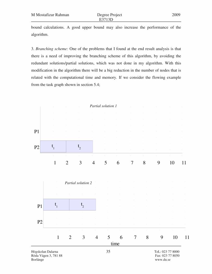
3. Branching scheme: One of the problems that I found at the end result analysis is that

there is a need of improving the branching scheme of this algorithm, by avoiding the

redundant solutions/partial solutions, which was not done in my algorithm. With this

modification in the algorithm there will be a big reduction in the number of nodes that is

related with the computational time and memory. If we consider the flowing example

from the task graph shown in section 5.4;

Partial solution 1

Partial solution 2


E3713D


Röda Vägen 3, 781 88 Fax: 023 77 8050

Borlänge www.du.se

36

1 2 3 4 5 6 7 8 9 10 11

P2

P1t1

t2

t1

t3

t4

t5

time

1 2 3 4 5 6 7 8 9 10 11

P2

P1 t3

time

t1

t2

t1

t4

t5

From the above chat of the partial solutions we can see that they are same just swapping

between the processors. One of them can easily be discarded for the further consideration

because they will lead to the same solutions which are shown below.

By doing this we can reduce the redundancy between the solutions as well as the can save

time and space not going with unnecessary branching.

Solution 1

Solution 1


E3713D


Röda Vägen 3, 781 88 Fax: 023 77 8050

Borlänge www.du.se

37

3. Coding and Data structure: efficient implementation of the algorithm with good

data structure will also save some time and space. The size of a node is very

important, in my implementation, a node structure is :

struct node{

int totalCPUTime; //to keep the the make span of the node

short int * schedule; // to keep the scheduling information

long *CPUStatus;// used to keep the status of the processor

long * taskStatus; // used to keep the status of a task

long numberOfUnscheduleTask; // number of unschedule task

long LB; //lower Bound

long UB; //upper Bound

long nodeNo; // unique number for identification of the node

struct node *next; // pointer to the next node

}

Now the size of the node will be

= (2*number of task) + (4*number of processor) + (4*number of task) +4+4+4+4+4+4

Bytes

I hope the size of the memory can also be reduced by finding a better structure of a node

having less size.

Finally to conclude the analysis I must say out of the above limitations the Lower Bound

is really important, and only an improved lower bound can give us the desired result.


E3713D


Röda Vägen 3, 781 88 Fax: 023 77 8050

Borlänge www.du.se

38

6.0 Conclusion and future work:

In this paper we tried to design a branch and bound algorithm for the multiprocessor

task scheduling problem. We have implemented two lower bounds for testing and

compare them with respect to time and numbers of node. We have tested the algorithm in

a small set of problem with less number of task and processor. There we find that LB2 is

performing better then the LB2. But one of the main problem that we found that this

algorithm is only applicable for small set of problem.

For the future work, I believe that there is a need of further improvement to find out a

new lower bound that will work for a bit large problem set, and also improvement of

coding may save memory and CPU time which will help to deal with large set of

problems. New branching scheme can also be proposed for betterment of the searching.

An interesting research can be made to find out the best solution using a hybrid

algorithm, combining genetic algorithms and integer programming branch and bound

approaches.


E3713D


Röda Vägen 3, 781 88 Fax: 023 77 8050

Borlänge www.du.se

39

References:

[1] Reakook Hwanga, Mitsuo Genb, Hiroshi Katayamaa. “A comparison of

multiprocessor task scheduling algorithms with communication costs” Science Direct

Computers & Operations Research 35 (2008) 976 – 993.

[2] Correa, R.C, Ferreira, A, Rebreyend, Pascal. “Integrating list heuristics into genetic

algorithms for multiprocessor scheduling”. Parallel and Distributed Processing, 1996.

Eighth IEEE Symposium on IEEE Comput. Soc. Press.

[3] Correa, R.C, Ferreira, A, Rebreyend. ” Scheduling multiprocessor tasks with genetic

algorithms”. Parallel and Distributed Systems, IEEE Transactions on IEE/IEEE, 1999.

Issn: 10459219.

[4] Parallel Lower and Upper Bounds for Large TSPs, a summary of André Rohe's thesis

(in English), will appear in ZAMM Volume 77, Supplement 2, pp. 429-432, 1997.

[5] A recursive branch and bound algorithm for the multidimensional knapsack problem

Wiley Periodicals. 2008. Volume 22 Issue 2, Pages 341 – 353

[6] Carlier J. Scheduling jobs with release dates and tails on identical parallel machines to

minimize the makespan. European Journal of Operational Research 1987;29:298–306.

[7] Carlier J, Pinson E. Jackson’s pseudo preemptive schedule for the P|ri, qi |Cmax.

Annals of Operations Research 1998;83:41–58.

[8] Gharbi A, Haouari M. Minimizing makespan on parallel machines subject to release

dates and delivery times. Journal of Scheduling 2002;5:329–55.

[9] Webster S-T. A general bound for the makespan problem. European Journal of

Operational Research 1996;89:516–24.

[10] Sang-Oh Shim,Yeong-Dae Kim. “A branch and bound algorithm for an identical

parallel machine scheduling problem with a job splitting property” Computers &

Operations Research 35 (2008) 863 – 875.

[11] Mohammad Mahdavi Mazdeha, Mansoor Sarhadia, Khalil S. Hindi”A branch-and-

bound algorithm for single-machine scheduling with batch delivery and job release

times” Computers & Operations Research 35 (2008) 1099 – 1111

[12] Rabia Nessah∗, FaroukYalaoui, Chengbin Chu.A “branch-and-bound algorithm to

minimize total weighted completion time on identical parallel machines with job release

dates.” Computers & Operations Research 35 (2008) 1176 – 1190

Branch and Bound Algorithm for Multiprocessor Scheduling

Documents

Transcript of Branch and Bound Algorithm for Multiprocessor Scheduling