Multipreconditioned GMRES for Shifted Systems

Tania Bakhos, Peter K. Kitanidis, Scott Ladenheim,

Arvind K. Saibaba, and Daniel B. Szyld

Report 16-03-31

March 2016

Department of Mathematics

Temple University

Philadelphia, PA 19122

This report is available in the World Wide Web at

http://www.math.temple.edu/~szyld

and also in the arxiv at http://arxiv.org/pdf/1603.08970v1.pdf

MULTIPRECONDITIONED GMRES FOR SHIFTED SYSTEMS⇤

TANIA BAKHOS†, PETER K. KITANIDIS†, SCOTT LADENHEIM‡,ARVIND K. SAIBABA§, AND DANIEL B. SZYLD¶

Abstract. An implementation of GMRES with multiple preconditioners (MPGMRES) is pro-posed for solving shifted linear systems with shift-and-invert preconditioners. With this type ofpreconditioner, the Krylov subspace can be built without requiring the matrix-vector product withthe shifted matrix. Furthermore, the multipreconditioned search space is shown to grow only linearlywith the number of preconditioners. This allows for a more e�cient implementation of the algorithm.The proposed implementation is tested on shifted systems that arise in computational hydrology andthe evaluation of di↵erent matrix functions. The numerical results indicate the e↵ectiveness of theproposed approach.

1. Introduction. We consider the solution of shifted linear systems of the form

(A+ �j

I)xj

= b, j = 1, . . . , n�

, (1.1)

where A 2 Rn⇥n is nonsingular, I is the n ⇥ n identity matrix, and n�

denotes thenumber of (possibly complex) shifts �

j

. We assume that the systems of equations (1.1)have unique solutions for j = 1, . . . , n

�

; i.e., for each �j

we assume (A+�j

I) is invert-ible. These types of linear systems arise in a wide range of applications, for instance,in quantum chromodynamics [8], hydraulic tomography [23], and in the evaluationof matrix functions based on the Cauchy integral formula [13]. Computing the so-lution to these large and sparse shifted systems remains a significant computationalchallenge in these applications.

For large systems, e.g, arising in the discretization of three-dimensional partialdi↵erential equations, solving these systems with direct methods, such as with sparseLU or Cholesky factorizations, is impractical, especially considering that a new fac-torization must be performed for each shift. An attractive option is the use of Krylovsubspace iterative methods. These methods are well-suited for the solution of shiftedsystems because they are shift-invariant; see, e.g., [27]. As a result of this propertyonly a single shift-independent Krylov basis needs to be generated from which allshifted solutions can be computed. In this paper we consider for its solution a variantof the generalized minimal residual method (GMRES) [22], since the matrix A in (1.1)is possibly nonsymmetric.

Preconditioning is essential to obtain fast convergence in a Krylov subspacemethod. It transforms the original linear system into an equivalent system with fa-vorable properties so that the iterative method converges faster. For shifted systems,preconditioning can be problematic because it may not preserve the shift-invariantproperty of Krylov subspaces. There are a few exceptions though, namely, poly-nomial preconditioners [1, 14], shift-and-invert preconditioners [11, 18, 19, 23], and

⇤This version dated March 29, 2016†Huang Engineering Center, Stanford University, Stanford, CA 94305 (taniab@stanford.edu,

peterk@stanford.edu).‡School of Computer Science, University of Manchester, Manchester, UK, M13 9PL

(scott.ladenheim@manchester.ac.uk).§Department of Mathematics, North Carolina State University, Raleigh, NC 27695

(asaibab@ncsu.edu).¶Department of Mathematics, Temple University, 1805 N Broad Street, Philadelphia, PA 19122

(szyld@temple.edu). This research is supported in part by the U.S. National Science Foundationunder grant DMS-1418882.

1

nested Krylov approaches [3]. Here, we consider using several shift-and-invert pre-conditioners of the form

P�1

j

= (A+ ⌧j

I)�1, (1.2)

where the values {⌧j

}np

j=1

correspond to the di↵erent shifts, with np

⌧ n�

. For

a generic shift ⌧ , we denote the preconditioner P�1

⌧

. One advantage of using thepreconditioner in (1.2) is that, as shown in the next section, the appropriate precon-ditioned Krylov subspace can be built without performing the matrix-vector productwith (A+ �

j

I).The reason to consider several shifted preconditioners is that a single precondi-

tioner alone is insu�cient to e↵ectively precondition across all shifts, as observed in[11, 23]. Incorporating more than one preconditioner necessitates the use of flexibleKrylov subspace methods; see, e.g., [21, 28, 29]. Flexible methods allow for the ap-plication of a di↵erent preconditioner at each iteration and the preconditioners arecycled in some pre-specified order. However, this means that information from onlyone preconditioner is added to the basis at each iteration. In addition, the order inwhich the preconditioners are applied can have a significant e↵ect on the convergenceof the iterative method. To e↵ectively precondition across the range of shifts we usemultipreconditioned GMRES (MPGMRES) [9].

Multipreconditioned Krylov subspace methods o↵er the capability of using sev-eral preconditioners at each iteration during the course of solving linear systems. Incontrast to flexible methods using one preconditioner at each iteration, the MPGM-RES approach uses information from all the preconditioners in every iteration. SinceMPGMRES builds a larger and richer search space, the convergence is expected to befaster than FGMRES. However, the cost per iteration for MPGMRES can be substan-tial. To deal with these large computational costs, and in particular the exponentialgrowth of the search space, a selective version of the algorithm is proposed in [9],where the growth of the search space is linear per iteration, i.e., the same growth asa block method of block size n

p

.Our major contribution is the development of a new iterative solver to handle

shifted systems of the form (1.1) that uses multiple preconditioners together withthe fact that no multiplication with (A + �

j

I) is needed. Our proposed method ismotivated by MPGMRES and builds a search space using information at each iterationfrom multiple shift-and-invert preconditioners. By searching for optimal solutions overa richer space, we anticipate the convergence to be rapid and the number of iterationsto be low. For this class of preconditioners, the resulting Krylov space has a specialform, and we show that the search space grows only linearly. This yields a methodwith contained computational and storage costs per iteration. Numerical experimentsillustrate that the proposed solver is more e↵ective than standard Krylov methods forshifted systems, in terms of both iteration counts and overall execution time.

We show that the proposed approach can also be applied to the solution of moregeneral shifted systems of the form (K + �M)x = b with shift-and-invert precondi-tioners of the form (K + ⌧M)�1; see Sections 3.3 and 4.

The paper is structured as follows. In Section 2, we briefly review some ba-sic properties of GMRES for the solution of shifted systems with shift-and-invertpreconditioners. We also review the MPGMRES algorithm, and a flexible GMRES(FGMRES) algorithm for shifted systems proposed in [23]. In Section 3, we presentthe proposed MPGMRES implementation for shifted systems with shift-and-invertpreconditioners, a new theorem characterizing the linear growth of the MPGMRES

2

search space, and discuss an e�cient implementation of the algorithm that exploitsthis linear growth. In Section 4, we present numerical experiments for shifted linearsystems arising in hydraulic tomography computations. In Section 5, we present an-other set of numerical experiments for the solution of shifted systems arising from theevaluation of di↵erent matrix functions. Concluding remarks are given in Section 6.

2. GMRES, MPGMRES, and FMGRES-Sh. To introduce the proposedmultipreconditioned approach for GMRES applied to shifted linear systems, the orig-inal GMRES algorithm [22], the multipreconditioned version MPGMRES [9], GMRESfor shifted systems, and flexible GMRES for shifted systems (FGMRES-Sh) [11, 23]are first reviewed.

2.1. GMRES. GMRES is a Krylov subspace iterative method for solving large,sparse, nonsymmetric linear systems of the form

Ax = b, A 2 Rn⇥n, b 2 Rn. (2.1)

From an initial vector x0

and corresponding residual r0

= b�Ax0

, GMRES computesat step m an approximate solution x

m

to (2.1) belonging to the a�ne Krylov subspacex0

+Km

(A, r0

), where

Km

(A, r0

) ⌘ Span{r0

, Ar0

, . . . , Am�1r0

}.

The corresponding residual rm

= b � Axm

is characterized by the minimal residualcondition

krm

k2

= minx2x0+Km(A,r0)

kb�Axk2

.

The approximate solution is the sum of the vector x0

and a linear combinationof the orthonormal basis vectors of the Krylov subspace, which are generated bythe Arnoldi algorithm. The first vector in the Arnoldi algorithm is the normalizedinitial residual v

1

= r0

/�, where � = kr0

k2

, and subsequent vectors vk

are formed byorthogonalizing Av

k�1

against all previous basis vectors. Collecting the basis vectorsinto the matrix V

m

= [v1

, . . . , vm

], one can write the Arnoldi relation

AVm

= Vm+1

Hm

, (2.2)

where Hm

2 Rm+1⇥m is an upper Hessenberg matrix whose entries are the orthogo-nalization coe�cients.

Thus, solutions of the form x = x0

+ Vm

ym

are sought for some ym

2 Rm. Usingthe Arnoldi relation, and the fact that V

m

is orthonormal, the GMRES minimizationproblem can be cast as the equivalent, smaller least-squares minimization problem

krm

k2

= miny2Rm

k�e1

� Hm

yk2

, (2.3)

with solution ym

, where e1

= [1, 0, . . . , 0]T is the first standard basis vector in Rm.

2.2. MPGMRES. The multipreconditioned GMRES method allows multiplepreconditioners to be incorporated in the solution of a given linear system. The methoddi↵ers from standard preconditioned Krylov subspace methods in that the approxi-mate solution is found in a larger and richer search space [9]. This multipreconditionedsearch space grows at each iteration by applying each of the preconditioners to all cur-rent search directions. In building this search space some properties of both flexible

3

and block Krylov subspace methods are used. As with GMRES, the MPGMRES algo-rithm then produces an approximate solution satisfying a minimal residual conditionover this larger subspace.

Computing the multi-Krylov basis is similar to computing the Arnoldi basis inGMRES but with a few key di↵erences. Starting from an initial vector x

0

, corre-sponding initial residual r

0

, and setting V (1) = r0

/�, the first MPGMRES iterate x1

is found in

x1

2 x0

+ Span{P�1

1

r0

, . . . , P�1

npr0

},

such that the corresponding residual has minimum 2-norm over all vectors of thisform. Equivalently, x

1

= x0

+ Z(1)y1

, where Z(1) = [P�1

1

r0

· · ·P�1

npr0

] 2 Rn⇥np andthe vector y

1

minimizes the residual. Note that the corresponding residual belongs tothe space

r1

2 r0

+ Span{AP�1

1

r0

, . . . , AP�1

npr0

}.

In other words, at the first iteration, the residual can be expressed as a first degreemultivariate (non-commuting) matrix polynomial with arguments AP�1

j

applied tothe initial residual, i.e.,

r1

= r0

+

npX

j=1

↵(1)

j

AP�1

j

r0

⌘ q1

(AP�1

1

, . . . , AP�1

np)r

0

,

with the property that q1

(0, . . . , 0) = 1.The next set of basis vectors V (2), with orthonormal columns, are generated by

orthogonalizing the columns of AZ(1) against V (1) = r0

/�, and performing a thin QRfactorization. The orthogonalization coe�cients generated in this process are storedin matrices H(j,1), j = 1, 2. The space of search directions is increased by applyingeach preconditioner to this new matrix; i.e., Z(2) = [P�1

1

V (2) . . . P�1

npV (2)] 2 Rn⇥n

2p .

The general procedure at step k is to block orthogonalize AZ(k) against the matricesV (1), . . . , V (k), and then performing a thin QR factorization to generate V (k+1) withorthonormal columns. By construction, the number of columns in Z(k), called searchdirections, and V (k), called basis vectors, is nk

p

.

Gathering all of the matrices, V (k), Z(k), and H(j,i) generated in the multipre-conditioned Arnoldi procedure into larger matrices yields a decomposition of the form

AZm

= Vm+1

Hm

, (2.4)

where

Zm

=⇥Z(1) · · · Z(m)

⇤, V

m+1

=⇥V (1) · · · V (m+1)

⇤,

and

Hm

=

2

666664

H(1,1) H(1,2) · · · H(1,m)

H(2,1) H(2,2) H(2,m)

. . .

H(m,m�1) H(m,m)

H(m+1,m)

3

777775·

4

Similar to the standard Arnoldi method, the matrix Hm

is upper Hessenberg. Intro-ducing the constant

⌃m

=mX

k=0

nk

p

=nm+1

p

� 1

np

� 1,

we have that

Zm

2 Rn⇥(⌃m�1), Vm+1

2 Rn⇥⌃m , Hm

2 R⌃m⇥(⌃m�1).

The multipreconditioned search space is spanned by the columns of Zm

so thatapproximate solutions have the form x

m

= x0

+ Zm

y for y 2 R⌃m�1. Thus, thanksto (2.4), MPGMRES computes y as the solution of the least squares problem

krm

k2

= miny2R⌃m�1

k�e1

� Hm

yk2

.

This is analogous to the GMRES minimization problem, except that here, alarger least squares problem is solved. Note that both Z

m

and Vm

are stored. Thecomplete MPGMRES method consists of the multipreconditioned Arnoldi procedurecoupled with the above least squares minimization problem. Furthermore, we high-light the expression of the MPGMRES residual as a multivariate polynomial, i.e.,we can write r

m

= qm

(AP�1

1

, . . . , AP�1

np)r

0

, where qm

(X1

, . . . , Xnp) 2 P

m

. HerePm

⌘ Pm

[X1

, . . . , Xnp ] is the space of non-commuting polynomials of degree m in

np

variables such that qm

(0, . . . , 0) = 1.In the above description of MPGMRES we have tacitly assumed that the ma-

trix Zm

is of full rank. However, in creating the multipreconditioned search space,columns of Z

m

may become linearly dependent. Strategies for detecting when suchlinear dependencies arise and then deflating the search space accordingly have beenproposed. For the implementation details of the complete MPGMRES method, aswell as information on selective variants for maintaining linear growth of the searchspace, we refer the reader to [9, 10].

2.3. GMRES for shifted systems. The solution of shifted systems using theGMRES method requires minor but important modifications. One key idea is to ex-ploit the shift-invariant property of Krylov subspaces, i.e., K

m

(A+�I, b) = Km

(A, b),and generate a single approximation space from which all shifted solutions are com-puted. For shifted systems, the Arnoldi relation is

(A+ �I)Vm

= Vm+1

✓H

m

+ �

Im

0

�◆⌘ V

m+1

Hm

(�), (2.5)

where Im

is the m ⇥ m identity matrix. The matrices Vm

, Hm

are the same as in(2.2) and are independent of the shift �.

Using (2.5), the equivalent shift-dependent GMRES minimization problem is

krm

(�)k2

= miny2Rm

k�e1

� Hm

(�)yk2

.

This smaller least squares problem is solved for each shift. Note that the computa-tionally intensive step of generating the basis vectors V

m

is performed only once andthe cheaper solution of the projected, smaller minimization problem occurs for eachof the shifts. We remark that the GMRES initial vector is x

0

= 0 for shifted systemssince the initial residual must be shift independent.

5

2.4. FGMRES for shifted systems. As previously mentioned, we considerusing several shift-and-invert preconditioners in the solution of shifted systems. Thisis due to the fact that a single shift-and-invert preconditioner is ine↵ective for pre-conditioning over a large range of shift values �, a key observation made in [11, 23].Using FMGRES, one can cycle through and apply P�1

j

for each value of ⌧j

. Incor-porating information from the di↵erent shifts into the approximation space improvesconvergence compared to GMRES with a single shifted preconditioner.

To build this approximation space the authors in [11] use the fact that

(A+ �I)(A+ ⌧I)�1 = I + (� � ⌧)(A+ ⌧I)�1, (2.6)

from which it follows that

Km

((A+ �I)P�1

⌧

, v) = Km

(P�1

⌧

, v). (2.7)

Therefore, they propose building a Krylov subspace based on P�1

⌧

. Note that theKrylov subspace K

m

(P�1

⌧

, v) is independent of � and therefore each shifted systemcan be projected onto this approximation space. The flexible approach constructs abasis Z

m

of the approximation space, where each column zj

= P�1

j

vj

corresponds toa di↵erent shift. This gives the following flexible, shifted Arnoldi relation

(A+ �I)Zm

= (A+ �I)[P�1

1

v1

· · ·P�1

m

vm

] = Vm+1

✓H

m

(�Im

� Tm

) +

Im

0

�◆,

where Tm

= diag(⌧1

, . . . , ⌧m

).Although this approach is more e↵ective than a single preconditioner, information

from only a single shift is incorporated into the search space at each iteration and theorder in which the preconditioners are applied can a↵ect the performance of FGMRES.These potential deficiencies motivate the proposed multipreconditioned algorithm,which allows for information from all preconditioners (i.e., all shifts ⌧

1

, . . . , ⌧m

) to bebuilt into the approximation space at every iteration.

3. MPGMRES for shifted systems. In this section, we present a modifi-cation of the MPGMRES algorithm to handle shifted systems with multiple shift-and-invert preconditioners, where the relation (2.7) plays a crucial role. The newalgorithm is referred to as MPGMRES-Sh. We shall prove that the growth of thesearch space at each iteration is linear in the number of preconditioners thereby lead-ing to an e�cient algorithm. This is in contrast to the original MPGMRES algorithmwhere the dimension of the search search space grows exponentially in the number ofpreconditioners.

The proposed implementation of MPGMRES for solving shifted systems (1.1)with preconditioners (1.2) adapts the flexible strategy of [23], and using relation (2.7)builds a shift-invariant multipreconditioned search space that is used to solve for eachshift. We assume throughout that (A+ ⌧

j

I) is invertible for all j = 1, . . . , np

so thatthe preconditioners P�1

j

= (A+ ⌧j

I)�1 are well-defined. The MPGMRES algorithm

proceeds by applying all np

preconditioners to the columns of V (k), which results in

Z(k) = [(A+ ⌧1

I)�1V (k), . . . , (A+ ⌧npI)

�1V (k)] 2 Rn⇥n

kp , V (k) 2 Rn⇥n

k�1p . (3.1)

Rearranging this we obtain the relation

AZ(k) + Z(k)T (k) = V (k)E(k), E(k) = eTnp

⌦ In

k�1p

, (3.2)

6

where eTnp

= [1, . . . , 1]| {z }np times

T and

T (k) = block diag

8>><

>>:⌧1

, . . . , ⌧1| {z }

n

k�1p times

, . . . , ⌧np , . . . , ⌧np| {z }n

k�1p times

9>>=

>>;2 Rn

kp⇥n

kp . (3.3)

Concatenating the matrices Z(k) and V (k) for k = 1, . . . ,m, into Zm

and Vm

, werewrite the m equations in (3.2) into a matrix relation

AZm

+ Zm

Tm

= Vm

Em

, (3.4)

where Tm

= block diag{T (1), . . . , T (m)} and Em

= block diag�E(1), . . . , E(m)

.

To generate the next set of vectors V (k+1) we use a block Arnoldi relationship ofthe form

V (k+1)H(k+1,k) = Z(k) �kX

j=1

V (j)H(j,k),

in combination with (3.1), so that at the end of m iterations, the flexible multipre-conditioned Arnoldi relationship holds, i.e., Z

m

= Vm+1

Hm

. In summary, we havethe system of equations

Zm

= Vm+1

Hm

, (3.5)

Zm

Tm

= Vm+1

Hm

Tm

, (3.6)

AZm

+ Zm

Tm

= Vm

Em

. (3.7)

Remark 3.1. From (2.6), it follows that Span{Zm

} = Span{(A + �I)Zm

}; seealso (2.7). As a consequence, in Step 4 of Algorithm 1 we do not need to explicitly

compute matrix-vector products with A.

Combining relations (3.5)–(3.7), we obtain the following flexible multiprecondi-tioned Arnoldi relationship for each shift �:

(A+ �I)Zm

= Vm+1

✓E

m

0

�+ H

m

(�I � Tm

)

◆⌘ V

m+1

Hm

(�;Tm

). (3.8)

Finally, searching for approximate solutions of the form xm

= Zm

ym

(recall thatx0

= 0) and using the minimum residual condition we have the following minimizationproblem for each shift:

krm

(�)k2

= minx2Span{Zm}

kb� (A+ �I)xm

k2

= miny2R⌃m�1

kb� (A+ �I)Zm

yk2

= miny2R⌃m�1

kVm+1

(�e1

� Hm

(�;Tm

)y)k2

= miny2R⌃m�1

k�e1

� Hm

(�;Tm

)yk2

.

(3.9)

The application of the multipreconditioned Arnoldi method using each preconditionerP�1

j

in conjunction with the solution of the above minimization problem is the com-plete MPGMRES-Sh method, see Algorithm 1.

7

Algorithm 1 Complete MPGMRES-Sh

Require: Matrix A, right-hand side b, preconditioners {A+ ⌧j

I}np

j=1

, shifts {�j

}n�j=1

,

{⌧j

}np

j=1

, and number of iterations m.

1: Compute � = kbk2

and V (1) = b/�.2: for k = 1, . . . ,m do3: Z(k) = [P�1

1

V (k), . . . , P�1

npV (k)]

4: W = Z(k)

5: for j = 1,. . . ,k do6: H(j,k) = (V (j))TW7: W = W � V (j)H(j,k)

8: end for9: W = V (k+1)H(k+1,k) {thin QR factorization}

10: end for11: for j = 1, . . . , n

�

do12: Compute y

m

(�j

) = argminy

k�e1

� Hm

(�j

;Tm

)yk for each shift.13: x

m

(�j

) = Zm

ym

(�j

), where Zm

= [Z(1), · · · , Z(m)]14: end for15: return The approximate solution x

m

(�j

) for j = 1, . . . , n�

.

3.1. Growth of the search space. It can be readily seen in Algorithm 1 thatthe number of columns of Z

m

and Vm

grows exponentially. However, as we shallprove below, with the use of shift-and-invert preconditioners the dimension of thisspace grows only linearly.

Noting that rm

(�) 2 Span{Vm+1

}, the residuals produced by the MPGMRES-Shmethod are of the form

rm

(�) 2 qm

(P�1

1

, . . . , P�1

np)b, (3.10)

for a polynomial qm

2 Pm

. Recall that Pm

is the space of multivariate polynomialsof degree m in n

p

(non-commuting) variables such that qm

(0, . . . , 0) = 1. Note thatthis polynomial is independent of the shifts �

j

.To illustrate this more clearly, for the case of n

p

= 2 preconditioners, the firsttwo residuals are of the form

r1

(�) 2 b+ ↵(1)

1

P�1

1

b+ ↵(1)

2

P�1

2

b,

r2

(�) 2 b+ ↵(2)

1

P�1

1

b+ ↵(2)

2

P�1

2

b+ ↵(2)

3

(P�1

1

)2b+ ↵(2)

4

P�1

1

P�1

2

b

+ ↵(2)

5

P�1

2

P�1

1

b+ ↵(2)

6

(P�1

2

)2b.

The crucial point we subsequently prove is that the cross-product terms of theform P�1

i

P�1

j

v 2 Span{P�1

i

v, P�1

j

v} for i 6= j. In particular, only the terms that

are purely powers of the form P�k

i

v need to be computed. This allows Span{Zm

} tobe expressed as the sum of Krylov subspaces generated by individual shift-and-invertpreconditioners P�1

i

; cf. (2.7). Thus, the search space has only linear growth in thenumber of preconditioners.

For ease of demonstration, we first prove this for np

= 2 preconditioners. Toprove the theorem we need the following two lemmas.

Lemma 3.2. Let P�1

1

, P�1

2

be shift-and-invert preconditioners as defined in (1.2)with ⌧

1

6= ⌧2

. Then P�1

1

P�1

2

v 2 Span{P�1

1

v, P�1

2

v}.8

Proof. We show there exist constants �1

, �2

such that

P�1

1

P�1

2

v = �1

P�1

1

v + �2

P�1

2

v = P�1

2

P�1

1

v. (3.11)

Setting v = P2

w and left multiplying by P1

gives the following equivalent formulation

w = �1

P2

w + �2

P1

w = �1

(A+ ⌧2

I)w + �2

(A+ ⌧1

I)w

= (�1

+ �2

)Aw + (�1

⌧2

+ �2

⌧1

)w.

By equating coe�cients we obtain that (3.11) holds for

�1

=1

⌧2

� ⌧1

= ��2

.

Remark 3.3. Note that P�1

1

P�1

2

= P�1

2

P�1

1

, i.e., the preconditioners commute

even though we have not assumed that A is diagonalizable. We make use of this

observation repeatedly.

Lemma 3.4. Let P�1

1

, P�1

2

be shift-and-invert preconditioners as defined in (1.2)with ⌧

1

6= ⌧2

, then

P�m

1

P�n

2

v 2 Km

(P�1

1

, P�1

1

v) +Kn

(P�1

2

, P�1

2

v).

Proof. We proceed by induction. The base case when m = n = 1 is true byLemma 3.2. Assume that the induction hypothesis is true for 1 j m, 1 k n,that is, we assume there exist coe�cients such that

P�m

1

P�n

2

v =mX

j=1

↵j

P�j

1

v +nX

j=1

↵0

j

P�j

2

v.

Now consider

P�(m+1)

1

P�(n+1)

2

v = (P�1

1

P�1

2

)(P�m

1

P�n

2

v)

=��1

P�1

1

+ �2

P�1

2

�0

@mX

j=1

↵j

P�j

1

v +nX

j=1

↵0

j

P�j

2

v

1

A

=m+1X

j=2

�1

↵j�1

P�j

1

v +n+1X

j=2

↵0

j�1

�2

P�j

2

v

+mX

j=1

↵j

�2

P�1

2

P�j

1

v +nX

j=1

�1

↵0

j

P�1

1

P�j

2

v

=m+1X

j=1

↵j

P�1

1

v +n+1X

j=1

↵0

j

P�1

2

v.

The first equality follows from the commutativity of P�1

1

and P�1

2

. The secondequality is the induction hypothesis. The third equality is just a result of the distribu-tive property. The final equality results from applications of Lemma 3.2 and thenexpanding and gathering like terms. It can be readily verified that every term in this

expression for P�(m+1)

1

P�(n+1)

2

v belongs to Km+1

(P�1

1

, P�1

1

v)+Kn+1

(P�1

2

, P�1

2

v).

9

Theorem 3.5. Let P�1

1

, P�1

2

be shift-and-invert preconditioners as defined in

(1.2) with ⌧1

6= ⌧2

. At the mthstep of the MPGMRES-Sh algorithm we have

rm

(�) = q(1)m

(P�1

1

)b+ q(2)m

(P�1

2

)b, (3.12)

where q(1)

m

, q(2)

m

2 Pm

[X] are such that q(1)

m

(0) + q(2)

m

(0) = 1. That is, the residual is

expressed as the sum of two (single-variate) polynomials of degree m on the appropriate

preconditioner, applied to b.Proof. Recall that at step m of the MPGMRES-Sh algorithm the residual can be

expressed as the multivariate polynomial (cf. (3.10))

rm

(�) = qm

(P�1

1

, P�1

2

)b, (3.13)

with qm

2 Pm

[X1

, X2

] and qm

(0, 0) = 1. Thus, we need only show that the multi-variate polynomial q

m

can be expressed as the sum of two polynomials in P�1

1

andP�1

2

. By Lemma 3.4, any cross-product term involving P�j

1

P�`

2

can be expressed asa linear combination of powers of only P�1

1

or P�1

2

. Therefore, gathering like termswe can express (3.13) as

rm

(�) =mX

j=1

↵j

P�j

1

b+mX

`=1

↵0

`

P�`

2

b = q(1)m

(P�1

1

)b+ q(2)m

(P�1

2

)b,

where q(i)

m

2 Pm

[X] and q(1)

m

(0) + q(2)

m

(0) = 1.For the general case of n

p

> 1, we have the same result, as stated below. Its proofis given in Appendix A.

Theorem 3.6. Let {P�1

j

}np

j=1

be shift-and-invert preconditioners as defined in

(1.2), where ⌧j

6= ⌧i

for j 6= i. At the mthstep of the MPGMRES-Sh algorithm we

have

rm

(�) =

npX

j=1

q(j)m

(P�1

j

)b,

where q(j)

m

2 Pm

[X] andP

np

j=1

q(j)

m

(0) = 1. In other words, the residual is a sum of

np

single-variate polynomials of degree m on the appropriate preconditioner, applied

to b.Remark 3.7. The residual can be equivalently expressed in terms of the Krylov

subspaces generated by the preconditioners P�1

j

and right hand side b:

rm

(�) 2 b+Km

(P�1

1

, P�1

1

b) + · · ·+Km

(P�1

np, P�1

npb).

Thus, at each iteration, the cross-product terms do not add to the search space and

the dimension of the search space grows linearly in the number of preconditioners.

3.2. Implementation details. As a result of Theorem 3.6, the MPGMRES-Shsearch space can be built more e�ciently than the original completeMPGMRES method. Although both methods compute the same search space, thecomplete MPGMRES method as described in Algorithm 1 builds a search space Z

m

withn

mp �np

np�1

columns. However, by Theorem 3.6, dim (Span{Zm

}) = mnp

, i.e., the

search space has only linear growth in the number of iterations and number of precon-ditioners. Thus, an appropriate implementation of complete MPGMRES-Sh applied

10

to our case would include deflating the linearly dependent search space; for exam-ple, using a strong rank-revealing QR factorization as was done in [9]. This processwould entail unnecessary computations, namely, in the number of applications of thepreconditioners, as well as in the orthonormalization and deflation.

These additional costs can be avoided by directly building the linearly growingsearch space. Implementing this strategy only requires appending to the matrix ofsearch directions Z

k�1

, np

orthogonal columns spanning R(Z(k)), the range of Z(k).Thus, only n

p

independent searh directions are needed. It follows from Theorem 3.6that any set of n

p

independent vectors in R(Zk

)\R(Zk�1

) su�ce. We generate thesevectors by applying each of the n

p

preconditioners to the last column of V (k).In other words, we replace step 3 in Algorithm 1 with

3’: Z(k) = [P�1

1

vk

, . . . , P�1

npvk

], where vk

= V (k)enp , (3.14)

and, where enp 2 Rnp⇥1 is the last column of the n

p

⇥np

identity matrix Inp . Note that

this implies that in line 12 the approximate solutions have the form xm

(�) = Zm

ym

(�)and the corresponding residual minimization problem is

krm

(�)k2

= miny2Rmnp

k�e1

� Hm

(�;Tm

)yk2

. (3.15)

Remark 3.8. Algorithm 1 with step 3’ as above is essentially what is called

selective MPGMRES in [9]. The big di↵erence here is that this “selective” version

captures the whole original search space (by Theorem 3.6), while in [9] only a subspace

of the whole search space is chosen.

This version of the algorithm is precisely the one we use in our numerical experi-ments. From (3.14) it can be seen that we need n

p

solves with a preconditioner periteration, and that at the kth iteration, one needs to perform

�k � 1

2

�n2

p

+ 3

2

np

innerproducts for the orthogonalization. This is in contrast to FGMRES-Sh where onlyone solve with a preconditioner per iteration is needed and only k+1 innere productsat the kth iteration. Nevertheless, as we shall see in sections 4 and 5, MPGMRES-Shachieves convergence in fewer iterations and lower computational times. The stor-age and computational cost of the MPGMRES-Sh algorithm is comparable to thatof a block Krylov method. The preconditioner solves can also be parallelized acrossmultiple cores, which further reduces the computational cost.

3.3. Extension to more general shifted systems. The proposed MPGMRES-Sh method, namely Algorithm 1 with step 3’ as in (3.14), can be easily adapted forsolving more general shifted systems of the form

(K + �j

M)x(�) = b, j = 1, . . . , n�

, (3.16)

with shift-and-invert preconditioners of the form Pj

= (K + ⌧j

M)�1, j = 1, . . . , np

.Using the identity

(K + �M)P�1

⌧

= (K + �M)(K + ⌧M)�1 = I + (� � ⌧)MP�1

⌧

, (3.17)

the same multipreconditioned approach described for the case M = I can be applied.The di↵erence for this more general case is that the multipreconditioned search spaceis now based on MP�1

⌧

.In this case, analogous to (3.1), we have

Z(k) = [(K + ⌧1

M)�1V (k), . . . , (K + ⌧t

M)�1V (k)] 2 Rn⇥n

kp , V (k) 2 Rn⇥n

k�1p ,

11

which is equivalently expressed as

KZ(k) +MZ(k)T (k) = V (k)E(k). (3.18)

Using (3.18) and concatenating Z(k), V (k), T (k), and E(k) into matrices we obtain thematrix relation

KZm

+MZm

Tm

= Vm

Em

, (3.19)

where Tm

and Em

are defined as in (3.4).Note that by (3.17), the multipreconditioned Arnoldi relationship holds, i.e.,

MZm

= Vm+1

Hm

, which in conjunction with (3.19) gives the general version of (3.8):

(K + �M)Zm

= Vm+1

✓E

m

0

�+ H

m

(�I � Tm

)

◆⌘ V

m+1

Hm

(�;Tm

).

As before, the approximate solutions have the form xm

(�) = Zm

ym

(�) and the cor-responding residual minimization problem is (3.15). It follows from (3.17) that onlya basis for the space Span{MZ

m

} needs to be computed. This is due to the shift-invariant property

Span{MZm

} = Span{(K + �M)Zm

}.

Thus, all we need to do is to use preconditioners of the form P�1

j

= (K + ⌧j

M)�1 inthe input to Algorithm 1 and replace step 4 in Algorithm 1 with

4’: W = MZ(k). (3.20)

We remark that the analysis and results of Theorem 3.6 remain valid for thesemore general shifted systems. To see this, consider the transformation of (3.16) to(KM�1 + �I)x

M

(�) = b by the change of variables xM

(�) = Mx(�). Note that thistransformation is only valid when M is invertible. As a result, we have a linear systemof the form (1.1) and all the previous results are applicable here. The analysis canbe extended to the case when M is not invertible; however, this is outside the scopeof this paper and is not considered here. For completeness, the resulting algorithm issummarized in Algorithm 2, which can be found in Appendix B.

3.4. Stopping criteria. We discuss here the stopping criteria used to test theconvergence of the solver. As was suggested by Paige and Saunders [20], we considerthe stopping criterion

krm

(�)k btol · kbk+ atol · kA+ �Ikkxm

(�)k. (3.21)

We found this criterion gave better performance on highly ill-conditioned matrices ascompared to the standard stopping criterion obtained by setting atol = 0. We canevaluate kx

m

(�)k using the relation kxm

(�)k = kZm

ym

(�)k. While we do not haveaccess to kA+ �Ik, we propose estimating it as follows

kA+ �Ik ⇡ maxk=1,...,mnp

|�k

| Hm

(�;Tm

)zk

= �k

Hm

zk

. (3.22)

The reasoning behind this approximation is that the solution of the generalized eigen-value problemH

m

(�;Tm

)zk

= �k

Hm

zk

are Harmonic Ritz eigenpairs, i.e., they satisfy

(A+ �I)u� ✓u ? Span{Vm

}, u 2 Span{Vm+1

Hm

};12

and therefore, can be considered to be approximate eigenvalues of A+ �I. The proofis a straightforward extension of [23, Proposition 1]. Numerical experiments confirmthat MPGMRES-Sh with the above stopping criterion does indeed converge to anacceptable solution and is especially beneficial for highly ill-conditioned matrices A.

Another modification to the stopping criterion needs to be made to account forinexact preconditioner solves. Following the theory developed in [26], a simple mod-ification was proposed in [23]. Computing the true residual would require an extraapplication of a matrix-vector product with A. Typically, this additional cost isavoided using the Arnoldi relationship and the orthogonality of V

m

to compute theresidual. However, when inexact preconditioners are used, the computed search spaceis a perturbation of the desired search space and the residual can only be computedapproximately. Assuming that the application of the inexact preconditioners has arelative accuracy ", based on [23], we use the modified stopping criterion

krm

(�)k btol · kbk+ atol · kA+ �Ikkxm

(�)k+ " · kym

(�)k1

, (3.23)

where ym

(�) is the solution of (3.9), i.e., step 12 of our algorithm, namely Algorithm 1with step 3’ as in (3.14) (or Algorithm 2 with K = A and M = I).

4. Application to Hydrology.

4.1. Background and motivation. Imaging the subsurface of the earth is animportant challenge in many hydrological applications such as groundwater remedi-ation and the location of natural resources. Oscillatory hydraulic tomography is amethod of imaging that uses periodic pumping tests to estimate important aquiferparameters, such as specific storage and conductivity. Periodic pumping signals areimposed at pumping wells and the transmitted e↵ects are measured at several ob-servation locations. The collected data is then used to yield a reconstruction of thehydrogeological parameters of interest. The inverse problem can be tackled using thegeostatistical approach; for details of this application see [23]. A major challenge insolving these inverse problems using the geostatistical approach is the cost of con-structing the Jacobian, which represents the sensitivity of the measurements to theunknown parameters. In [23], it is shown that constructing the Jacobian requiresrepeated solution to a sequence of shifted systems. An e�cient solver for the for-ward problem can drastically reduce the overall computational time required to solvethe resulting inverse problem. In this section, we demonstrate the performance ofMPGMRES-Sh for solving the forward problem with a periodic pumping source.

The equations governing groundwater flow through an aquifer for a given domain⌦ with boundary @⌦ = @⌦

D

[ @⌦N

[ ⌦W

are given by

Ss

(x)@�(x, t)

@t�r · (K(x)r�(x, t)) = q(x, t) x 2 ⌦, (4.1)

�(x, t) = 0 x 2 @⌦D

,

r�(x, t) · n = 0 x 2 @⌦N

K(x) (r�(x, t) · n) = Sy

@�(x, t)

@tx 2 @⌦

W

where Ss

(x) (units of L�1) represents the specific storage, Sy

(dimensionless) rep-resents the specific yield and K(x) (units of L/T ) represents the hydraulic conduc-tivity. The boundaries @⌦

D

, @⌦N

, and @⌦W

represent Dirichlet, Neumann, and the

13

linearized water table boundaries, respectively. In the case of one source oscillatingat a fixed frequency ! (units of radians/T) , q(x, t) is given by

q(x, t) = Q0

�(x� xs

) cos(!t).

We assume the source to be a point source oscillating at a known frequency ! andpeak amplitude Q

0

at the source location xs

. Since the solution is linear in time, weassume the solution (after some initial time has passed) can be represented as

�(x, t) = <(�(x) exp(i!t)),

where <(·) is the real part and �(x), known as the phasor, is a function of space onlythat contains information about the phase and amplitude of the signal. Assumingthis form of the solution, the equations (4.1) in the so-called phasor domain are

�r · (K(x)r�(x)) + i!Ss

(x)�(x) = Q0

�(x� xs

) x 2 ⌦, (4.2)

�(x) = 0 x 2 @⌦D

,

r�(x) · n = 0 x 2 @⌦N

,

K(x) (r�(x) · n) = i!Sy

�(x) x 2 @⌦W

.

The di↵erential equation (4.2) along with the boundary conditions are discretizedusing standard finite elements implemented through the FEniCS software package [15,16, 17]. Solving the discretized equations for several frequencies results in solvingsystems of shifted equations of the form

(K + �j

M)xj

= b j = 1, . . . , n�

, (4.3)

where, K and M are the sti↵ness and mass matrices, respectively. The relevantMPGMRES-Sh algorithm for this system of equations is the one described in Sec-tion 3.3, and summarized in Algorithm 2.

4.2. Numerical examples. In this section, we consider two synthetic aquifersin our test problems. In both examples, the equations are discretized using standardlinear finite elements implemented using FEniCS and Python as the user-interface.The first example is a two-dimensional depth-averaged aquifer in a rectangular do-main discretized using a regular grid. The second test problem is a challenging 3-Dsynthetic example chosen to reflect the properties observed at the Boise Hydrogeo-logical Research Site (BHRS) [5]; see Figure 4.1. Although the domain is regular,modeling the pumping well accurately requires the use of an unstructured grid. Thenumerical experiments were all performed on an HP workstation with 16 core IntelXeon E5-2687W (3.1 GHZ) processor running Ubuntu 14.04. The machine has 128GB RAM and 1 TB hard disk space.

4.2.1. Test Problem 1. We consider a two-dimensional aquifer in a rectangulardomain with Dirichlet boundary conditions on all boundaries. The log conductivityis chosen to be a random field generated from the Gaussian process N (µ(x),(x, y)),where (·, ·) is an exponential kernel taking the form

(x, y) = 4 exp

✓�2kx� yk

2

L

◆, (4.4)

with µ(x) the mean of the log-conductivity chosen to be constant and L the length ofthe aquifer domain. Other parameters for the model are summarized in Table 4.1; see

14

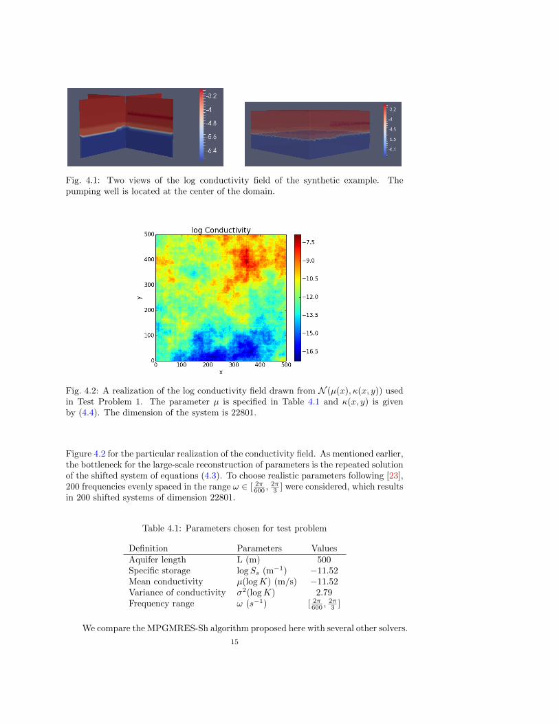
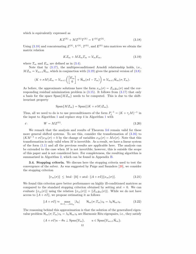
Fig. 4.1: Two views of the log conductivity field of the synthetic example. Thepumping well is located at the center of the domain.

Fig. 4.2: A realization of the log conductivity field drawn from N (µ(x),(x, y)) usedin Test Problem 1. The parameter µ is specified in Table 4.1 and (x, y) is givenby (4.4). The dimension of the system is 22801.

Figure 4.2 for the particular realization of the conductivity field. As mentioned earlier,the bottleneck for the large-scale reconstruction of parameters is the repeated solutionof the shifted system of equations (4.3). To choose realistic parameters following [23],200 frequencies evenly spaced in the range ! 2 [ 2⇡

600

, 2⇡

3

] were considered, which resultsin 200 shifted systems of dimension 22801.

Table 4.1: Parameters chosen for test problem

Definition Parameters ValuesAquifer length L (m) 500Specific storage logS

s

(m�1) �11.52Mean conductivity µ(logK) (m/s) �11.52Variance of conductivity �2(logK) 2.79Frequency range ! (s�1) [ 2⇡

600

, 2⇡

3

]

We compare the MPGMRES-Sh algorithm proposed here with several other solvers.

15

We consider the ‘Direct’ approach, which corresponds to solving the system for eachfrequency using a direct solver. Since this requires factorizing a matrix for each fre-quency, this is expensive. ‘GMRES-Sh’ refers to using preconditioned GMRES tosolve the shifted system of equations using a single shift-and-invert preconditioner,with the frequency chosen to be the midpoint of the range of frequencies. While this isnot the optimal choice of preconditioner, it is a representative example for illustratingthat one preconditioner does not e↵ectively precondition all systems. We also providea comparison with ‘FGMRES-Sh’. Following [23], we choose preconditioners of theform K + ⌧

k

M for k = 1, ...,m, where m is the maximum dimension of the Arnoldiiteration. Let ⌧ = {⌧

1

, . . . , ⌧np} be the list of values that ⌧

k

can take with np

denotingthe number of distinct preconditioners used. In [23], it is shown that systems withfrequencies nearer to the origin converge slower, so we choose the values of ⌧ to beevenly spaced in a log scale in the frequency range ! 2 [ 2⇡

600

, 2⇡

3

]. For FGMRES-Shwith n

p

preconditioners we assign the first m/np

values of ⌧k

as ⌧1

, the next m/np

values of ⌧k

to ⌧2

and so on. If the algorithm has not converged in m iterations, wecycle over the same set of preconditioners. ‘MPGMRES-Sh’ uses the same precondi-tioners as ‘FGMRES-Sh’ but builds a di↵erent search space. We set the size of thebases per preconditioner to be 5, i.e., m/n

p

= 5. A relative residual of less than 10�10

was chosen as the stopping criterion for all the iterative solvers, i.e., atol was set to 0.Furthermore, all the preconditioner solves were performed using direct solvers andcan be treated as exact in the absence of round-o↵ errors.

We report the results of the various aforementioned solvers in Figure 4.3. Inthe top two plots, we compare MPGMRES-Sh with FGMRES-Sh and we see that theiteration count to reach the desired tolerance is less with MPGMRES-Sh than with theuse of FGMRES-Sh. The vertical lines on the plot denote the preconditioners chosenin the case when n

p

= 5. In the bottom plot, we compare the solution times (inseconds) of the solvers to solve the 200 shifted systems. We observe that the ‘Direct’method is computationally prohibitive because the growth is linear with the numberof shifted systems. GMRES-Sh uses the shift-invariance property but the convergencewith each frequency is di↵erent and the number of iterations for some frequencies canbe quite large. Both FMRES-Sh and MPGMRES-Sh appear to behave independentlyof the number of shifted systems to be solved and MPGMRES-Sh converges marginallyfaster.

4.2.2. Test Problem 2. We now compare the solution time for a realistic 3-D problem on an unconfined aquifer. The aquifer is of size 60 ⇥ 60 ⇥ 27 m3 andthe pumping well is located in the center with the pumping occurring over a 1minterval starting 2m below the water table. For the free surface boundary (top), weuse the linearized water table boundary @⌦

W

; for the other boundaries we use ano-flow boundary for the bottom surface @⌦

N

and Dirichlet boundary conditions forthe side walls @⌦

D

. The dimension of the sparse matrices K and M is 132089 withapproximately 1.9 million nonzero entries each (both matrices have the same sparsitypattern). The number of shifts �

j

chosen is 100 with the periods evenly spaced inrange from 10 seconds to 15 minutes, resulting in ! 2 [ 2⇡

900

, 2⇡

10

]. Since the ‘Direct’ and‘GMRES-Sh’ approaches are infeasible on problems of this size, we do not providecomparisons with them. We focus on studying the iteration counts and time taken byFGMRES-Sh and MPGMRES-Sh. The choice of preconditioners and the constructionof basis for FGMRES-Sh and MPGMRES-Sh are the same as that for the previousproblem. The number of preconditioners n

p

is varied in the range 2–5. However, onecrucial di↵erence is that the preconditioner solves are now done using an iterative

16

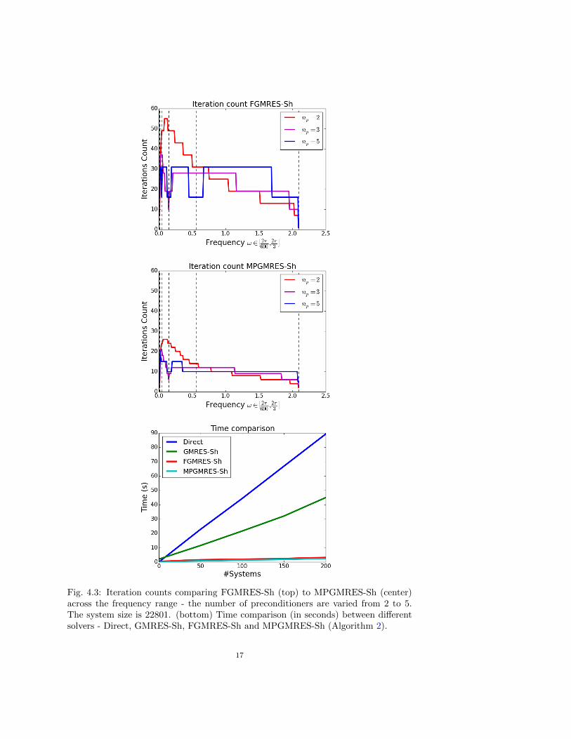
Fig. 4.3: Iteration counts comparing FGMRES-Sh (top) to MPGMRES-Sh (center)across the frequency range - the number of preconditioners are varied from 2 to 5.The system size is 22801. (bottom) Time comparison (in seconds) between di↵erentsolvers - Direct, GMRES-Sh, FGMRES-Sh and MPGMRES-Sh (Algorithm 2).

17

method, specifically, preconditioned CG with an algebraic multigrid (AMG) solveras a preconditioner available through the PyAMG package [4]. Following [23], thestopping criterion used for the preconditioner solve required the relative residual tobe less than 10�12. The number of iterations and the CPU time taken by FGMRES-Shand MPGMRES-Sh have been displayed in Table 4.2; as can be seen, MPGMRES-Shhas the edge over FGMRES-Sh both in iteration counts and CPU times. In Figure 4.4we report on the number of iterations for the di↵erent shifted systems.

Table 4.2: Comparison of MPGMRES-Sh with FGMRES-Sh on Test Problem 2.

np

FGMRES-Sh MPGMRES-ShMatvecs CPU Time [s] Matvecs CPU Time [s]

2 58 160.3 36 87.03 52 130.3 24 52.15 44 104.2 20 36.7

Fig. 4.4: Variation of iteration count with increasing number of preconditioners inMPGMRES-Sh (Algorithm 2) for Test Problem 2. The preconditioners are chosen ona log scale and their locations are highlighted in dashed lines.

5. Matrix Functions. Matrix function evaluations are relevant in many appli-cations; for example, the evaluation of exp(�tA)b is important in the time-integrationof large-scale dynamical systems [2]. In the field of statistics and uncertainty quantifi-cation, several computations involving a symmetric positive definite covariance matrixA can be expressed in terms of matrix functions. For example, evaluation of A1/2⇠can be used to sample from N (0, A) where ⇠ ⇠ N (0, I) as was implemented in [24],and an unbiased estimator to log (det(A)) can be constructed as

log (det(A)) = trace (log(A)) ⇡ 1

ns

nsX

k=1

⇣Tk

log(A)⇣k

,

18

where ⇣k

is drawn i.i.d. from a Rademacher or Gaussian distribution [25]. The eval-uation of the matrix function can be carried out by representing the function as acontour integral

f(A) =1

2⇡i

Z

�

f(z)(zI �A)�1dz,

where � is a closed contour lying in the region of analyticity of f . The matrix A isassumed to be positive definite and we consider functions f that are analytic exceptfor singularities or a branch cut on (or near) (�1, 0]. We consider the approachin [12] that uses a conformal map combined with the trapezoidal rule to achieve anexponentially convergent quadrature rule as the number of quadrature nodes N ! 1.The evaluation of the matrix function f(A)b can then be approximated by the sum

f(A)b ⇡ fN

(A)b =NX

j=1

wj

(zj

I �A)�1b, (5.1)

where wk

and zk

are quadrature weights and nodes. The convergence of the approxi-mation as N ! 1 is given by an expression of the type

kf(A)� fN

(A)k = O⇣e�C1⇡

2N/(log(M/m)+C2)

⌘,

where C1

and C2

are two constants depending on the particular method used andm,M are the smallest and largest eigenvalue of A, respectively [12]. Given a tolerance✏, we choose N according to the formula

N =

⇠(log(M/m) + C

2

)

C1

⇡2✏

⇡.

In our application, we choose ✏ = 10�6, so that the expression (5.1) requires thesolution of shifted system of equations (z

j

I � A)xj

= b for j = 1, . . . , N and can becomputed e�ciently using the MPGMRES-Sh algorithm. Note that N depends onthe function f(·) and the condition number of the matrix A.

For these experiments we used the stopping criterion in Section 3.4 with atol= btol = 10�10. Three preconditioners were used with shifts at z

1

, zN/2

, and zN

.For FGMRES-Sh, we use the same strategy to cycle through the preconditioners.Furthermore, m/n

p

was set to be 5.We focus on evaluating the following three important matrix functions exp(�A),

log(A) and A1/2, and in each case we evaluate f(A)b for a randomly generated vectorof appropriate dimension. For exp(�A)b evaluation, we use Method 1, whereas forlog(A)b we use Method 2, and finally for A1/2 we use Method 3 as described in [12]. Wetake several matrices from the UF sparse matrix collection [7], which have previouslybeen studied in the context of computing matrix functions in [6]. The number ofiterations taken by FGMRES-Sh and MPGMRES-Sh is provided in Table 5.1. Ascan be seen, MPGMRES-Sh takes fewer preconditioner solves (recall that the matrix-vector products with the shifted matrices are not necessary) to converge to the desiredtolerance. The CPU times reported are averaged over 5 independent runs to getaccurate timing results. In these examples, as in the hydrology examples, MPGMRES-Sh is more e↵ective both in terms of iteration count and overall run time.

19

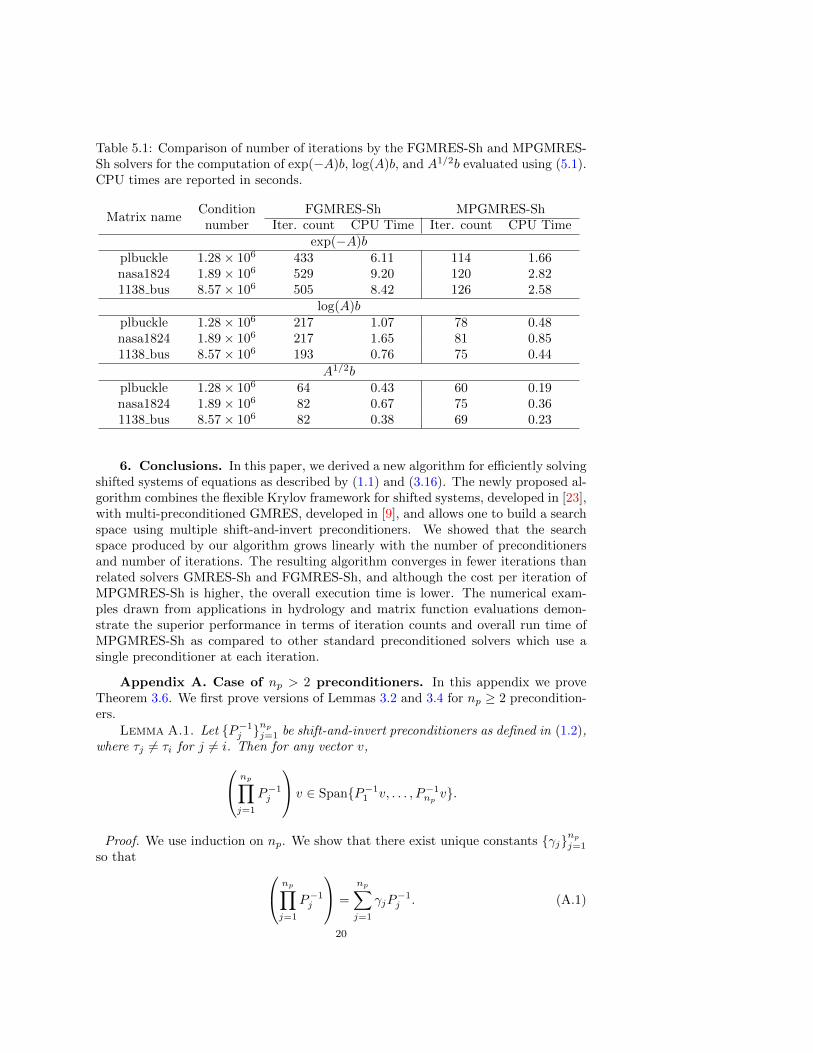
Table 5.1: Comparison of number of iterations by the FGMRES-Sh and MPGMRES-Sh solvers for the computation of exp(�A)b, log(A)b, and A1/2b evaluated using (5.1).CPU times are reported in seconds.

Matrix nameCondition FGMRES-Sh MPGMRES-Shnumber Iter. count CPU Time Iter. count CPU Time

exp(�A)bplbuckle 1.28⇥ 106 433 6.11 114 1.66nasa1824 1.89⇥ 106 529 9.20 120 2.821138 bus 8.57⇥ 106 505 8.42 126 2.58

log(A)bplbuckle 1.28⇥ 106 217 1.07 78 0.48nasa1824 1.89⇥ 106 217 1.65 81 0.851138 bus 8.57⇥ 106 193 0.76 75 0.44

A1/2bplbuckle 1.28⇥ 106 64 0.43 60 0.19nasa1824 1.89⇥ 106 82 0.67 75 0.361138 bus 8.57⇥ 106 82 0.38 69 0.23

6. Conclusions. In this paper, we derived a new algorithm for e�ciently solvingshifted systems of equations as described by (1.1) and (3.16). The newly proposed al-gorithm combines the flexible Krylov framework for shifted systems, developed in [23],with multi-preconditioned GMRES, developed in [9], and allows one to build a searchspace using multiple shift-and-invert preconditioners. We showed that the searchspace produced by our algorithm grows linearly with the number of preconditionersand number of iterations. The resulting algorithm converges in fewer iterations thanrelated solvers GMRES-Sh and FGMRES-Sh, and although the cost per iteration ofMPGMRES-Sh is higher, the overall execution time is lower. The numerical exam-ples drawn from applications in hydrology and matrix function evaluations demon-strate the superior performance in terms of iteration counts and overall run time ofMPGMRES-Sh as compared to other standard preconditioned solvers which use asingle preconditioner at each iteration.

Appendix A. Case of np

> 2 preconditioners. In this appendix we proveTheorem 3.6. We first prove versions of Lemmas 3.2 and 3.4 for n

p

� 2 precondition-ers.

Lemma A.1. Let {P�1

j

}np

j=1

be shift-and-invert preconditioners as defined in (1.2),where ⌧

j

6= ⌧i

for j 6= i. Then for any vector v,

0

@npY

j=1

P�1

j

1

A v 2 Span{P�1

1

v, . . . , P�1

npv}.

Proof. We use induction on np

. We show that there exist unique constants {�j

}np

j=1

so that0

@npY

j=1

P�1

j

1

A =

npX

j=1

�j

P�1

j

. (A.1)

20

holds for any integer np

. The proof for np

= 1 is straightforward. Assume (A.1) holdsfor n

p

> 1. For np

+ 10

@np+1Y

j=1

P�1

j

1

A =

0

@npY

j=1

P�1

j

1

AP�1

np+1

=

0

@npX

j=1

�j

P�1

j

1

AP�1

np+1

.

The last equality follows because of the induction hypothesis. Next, assuming that⌧np+1

6= ⌧j

for j = 1, . . . , np

, we use Lemma 3.4 to simplify the expression

npX

j=1

�j

P�1

j

P�1

np+1

=

npX

j=1

�j

⇣�(j)

1

P�1

j

+ �(j)

2

P�1

np+1

⌘

=

npX

j=1

�j

�(j)

1

P�1

j

+

0

@npX

j=1

�j

�(j)

2

1

AP�1

np+1

⌘np+1X

j=1

�0

j

P�1

j

.

Lemma A.2. Let {P�1

j

}np

j=1

be shift-and-invert preconditioners as defined in (1.2)where ⌧

j

6= ⌧i

for j 6= i. Then, for all vectors v and all integers m,

0

@npY

j=1

P�m

j

1

A v 2npX

j=1

Km

(P�1

j

, P�1

j

v).

Proof. We proceed by induction on m. The cases when m = 1 is true byLemma A.1. Assume that the Lemma holds for m > 1, i.e., there exist coe�cientssuch that

npY

k=1

P�m

k

!v =

mX

j=1

↵(j)

1

P�j

1

v + · · ·+mX

j=1

↵(j)

npP�j

npv.

Next, consider

npY

k=1

P�(m+1)

k

!v =

npY

k=1

P�1

k

! npY

k=1

P�m

k

!v

=

npY

k=1

P�1

k

!0

@mX

j=1

↵(j)

1

P�j

1

v + · · ·+mX

j=1

↵(j)

npP�j

npv

1

A

=mX

j=1

↵(j)

1

npY

k=1

P�1

k

!P�j

1

v + · · ·+mX

j=1

↵(j)

np

npY

k=1

P�1

k

!P�j

npv.

The first equality is a result of the commutativity of the shift-and-invert precondi-tioners. The second equality follows from the application of the induction hypothesis.Next, consider the last expression, which we rewrite as

npX

i=1

mX

j=1

↵(j)

i

P�j

i

npY

k=1

P�1

k

!v =

npX

i=1

mX

j=1

↵(j)

i

P�j

i

npX

k=1

�k

P�1

k

v

!

=

npX

i=1

mX

j=1

npX

k=1

↵(j)

i

�k

P�j

i

P�1

k

v,

21

where the first equality follows from an application of Lemma A.1. By repeatedapplication of Lemma 3.4, the Lemma follows.

Proof of Theorem 3.6. Recall that by (3.10) the residual can be expressed as amultivariate-polynomial in the preconditioners. Due to Lemma A.2, any cross-productterm can be reduced to a linear combination of powers only of P�1

j

. Gathering liketerms together, the residual can be expressed as a sum of single-variate polynomialsin each preconditioner.

Appendix B. Algorithm for more general shifted systems. For conve-nience, we provide the selective version of the algorithm for solving (3.16). Thespecial case for (1.1) can be obtained by setting K = A and M = I.

Algorithm 2 Selective MPGMRES-Sh for (3.16)

Require: MatricesK andM , right-hand side b, preconditioners {K+⌧j

M}np

j=1

, shifts

{�j

}n�j=1

, {⌧j

}np

j=1

and number of iterations m.

1: Compute � = kbk2

and V (1) = b/�.2: for k = 1, . . . ,m do3: v

k

= V (k)enp , and Z(k) = [P�1

1

vk

, . . . , P�1

npvk

].

4: W = MZ(k)

5: for j = 1,. . . ,k do6: H(j,k) = (V (j))TW7: W = W � V (j)H(j,k)

8: end for9: W = V (k+1)H(k+1,k) {thin QR factorization}

10: end for11: for j = 1, . . . , n

�

do12: Compute y

m

(�j

) = argminy

k�e1

� Hm

(�j

;Tm

)yk for each shift.13: x

m

(�j

) = Zm

ym

(�j

), where Zm

= [Z(1), · · · , Z(m)]14: end for15: return The approximate solution x

m

(�j

) for j = 1, . . . , n�

.

REFERENCES

[1] M. I. Ahmad, D. B. Szyld, and M. B. van Gijzen. Preconditioned multishift BiCG for H2-optimal model reduction. Technical Report 12-06-15, Department of Mathematics, TempleUniversity, June 2012. Revised March 2013 and June 2015.

[2] T. Bakhos, A. K. Saibaba, and P. K. Kitanidis. A fast algorithm for parabolic PDE-basedinverse problems based on laplace transforms and flexible Krylov solvers. Journal of Com-putational Physics, 299:940–954, 2015.

[3] M. Baumann and M. B. van Gijzen. Nested Krylov methods for shifted linear systems. SIAMJournal on Scientific Computing, 37(5):S90–S112, 2015.

[4] W. Bell, L. Olson, and J. Schroder. PyAMG: Algebraic multigrid solvers in Python v2. 0, 2011.URL http://www. pyamg. org. Release, 2, 2011.

[5] M. Cardi↵, W. Barrash, and P. K. Kitanidis. Hydraulic conductivity imaging from 3-d tran-sient hydraulic tomography at several pumping/observation densities. Water ResourcesResearch, 49(11):7311–7326, 2013.

[6] J. Chen, M. Anitescu, and Y. Saad. Computing f(A)b via least squares polynomial approxi-mations. SIAM Journal on Scientific Computing, 33:195–222, 2011.

[7] T. A. Davis and Y. Hu. The University of Florida sparse matrix collection. ACM Transactionson Mathematical Software, 38:1, 2011.

[8] A. Frommer, B. Nockel, S. Gusken, T. Lippert, and K. Schilling. Many masses on one stroke:

22

Economic computation of quark propagators. International Journal of Modern Physics C,6:627–638, 1995.

[9] C. Greif, T. Rees, and D. B. Szyld. MPGMRES: a generalized minimum residual method withmultiple preconditioners. Technical Report 11-12-23, Department of Mathematics, TempleUniversity, Dec. 2011. Revised September 2012, January 2014, and March 2015. Alsoavailable as Technical Report TR-2011-12, Department of Computer Science, University ofBritish Columbia.

[10] C. Greif, T. Rees, and D. B. Szyld. Additive Schwarz with variable weights. In J. Erhel,M. Gander, L. Halpern, G. Pichot, T. Sassi, and O. Widlund, editors, Domain Decompo-sition Methods in Science and Engineering XXI, Lecture Notes in Computer Science andEngineering, pages 661–668. Springer, Berlin and Heidelberg, 2014.

[11] G.-D. Gu, X.-L. Zhou, and L. Lin. A flexible preconditoned Arnoldi method for shifted linearsystems. Journal of Computational Mathematics, 25, 2007.

[12] N. Hale, N. J. Higham, and L. N. Trefethen. Computing A↵, log(A), and related matrixfunctions by contour integrals. SIAM Journal on Numerical Analysis, 46:2505–2523, 2008.

[13] N. J. Higham and A. H. Al-Mohy. Computing matrix functions. Acta Numerica, 19:159–208,2010.

[14] B. Jegerlehner. Krylov space solvers for shifted linear systems. arXiv preprint hep-lat/9612014,1996.

[15] A. Logg, K.-A. Mardal, G. N. Wells, et al. Automated Solution of Di↵erential Equations bythe Finite Element Method. Springer, 2012.

[16] A. Logg and G. N. Wells. DOLFIN: Automated finite element computing. ACM Transactionson Mathematical Software, 37, 2010.

[17] A. Logg, G. N. Wells, and J. Hake. DOLFIN: a C++/Python Finite Element Library, chap-ter 10. Springer, 2012.

[18] K. Meerbergen. The solution of parametrized symmetric linear systems. SIAM Journal onMatrix Analysis and Applications, 24:1038–1059, 2003.

[19] K. Meerbergen and Z. Bai. The Lanczos method for parameterized symmetric linear sys-tems with multiple right-hand sides. SIAM Journal on Matrix Analysis and Applications,31:1642–1662, 2010.

[20] C. C. Paige and M. A. Saunders. LSQR: An algorithm for sparse linear equations and sparseleast squares. ACM Transactions on Mathematical Software, 8:43–71, 1982.

[21] Y. Saad. A flexible inner-outer preconditioned GMRES algorithm. SIAM Journal on ScientificComputing, 14:461–469, 1993.

[22] Y. Saad and M. H. Schultz. GMRES: A generalized minimal residual algorithm for solvingnonsymmetric linear systems. SIAM Journal on Scientific and Statistical Computing,7:856–869, 1986.

[23] A. K. Saibaba, T. Bakhos, and P. K. Kitanidis. A flexible Krylov solver for shifted systems withapplication to oscillatory hydraulic tomography. SIAM Journal on Scientific Computing,35:A3001–A3023, 2013.

[24] A. K. Saibaba and P. K. Kitanidis. E�cient methods for large-scale linear inversion using ageostatistical approach. Water Resources Research, 48, 2012.

[25] A. K. Saibaba and P. K. Kitanidis. Fast computation of uncertainty quantification measuresin the geostatistical approach to solve inverse problems. Advances in Water Resources,82:124 – 138, 2015.

[26] V. Simoncini and D. B. Szyld. Theory of inexact Krylov subspace methods and applicationsto scientific computing. SIAM Journal on Scientific Computing, 25:454–477, 2003.

[27] V. Simoncini and D. B. Szyld. Recent computational developments in Krylov subspace methodsfor linear systems. Numerical Linear Algebra with Applications, 14:1–59, 2007.

[28] D. B. Szyld and J. A. Vogel. A flexible quasi-minimal residual method with inexact precondi-tioning. SIAM Journal on Scientific Computing, 23:363–380, 2001.

[29] J. A. Vogel. Flexible BiCG and flexible Bi-CGSTAB for nonsymmetric linear systems. AppliedMathematics and Computation, 188:226–233, 2007.

23