Multiple imputation using

ICE: A simulation study

on a binary response

Jochen Hardt

Kai Görgen

6th German Stata Meeting, Berlin June, 27th 2008

Göteborg UniversityUniversity of Mainz,Bernsteincenter for Computational Neuroscience, Berlin

•        Almost all sociological / medical data have missings- typically in the range of .5 to 5 % in a variable

Many statistical procedures can only use cases without missings

What we already know about missing substitution:

1) With a small amount of missings everything is easy2) Large samples are easy

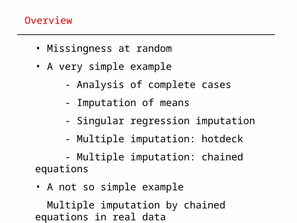
• Missingness at random

• A very simple example

- Analysis of complete cases

- Imputation of means

- Singular regression imputation

- Multiple imputation: hotdeck

- Multiple imputation: chained equations

• A not so simple example

Multiple imputation by chained equations in real data

Overview

There is a distinction in the literature about data being missing

completely at random (MCAR), missing at random (MAR) or being

missing not at random (Rubin, 1996).

MCAR means that the pattern of missings is totally at random, not

depending on any variable in or not in the analysis.

MAR is an intuitively somewhat misleading label, because it allows

strong dependencies in the pattern of missings. If, for example, in a

set of variables all data for men are missing and for women are non-

missing, the dataset is still MAR as long as gender is included as a

variable. The formal definition is that missings are at random given all

information available in the dataset.

Background I

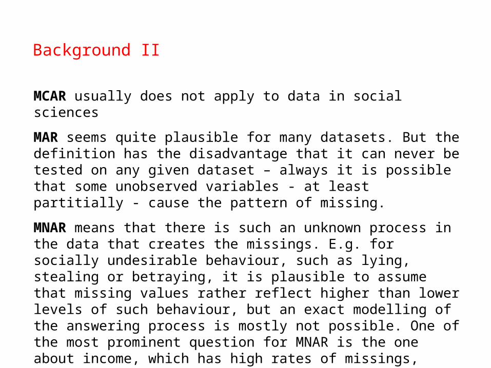
MCAR usually does not apply to data in social sciences

MAR seems quite plausible for many datasets. But the definition has the disadvantage that it can never be tested on any given dataset – always it is possible that some unobserved variables - at least partitially - cause the pattern of missing.

MNAR means that there is such an unknown process in the data that creates the missings. E.g. for socially undesirable behaviour, such as lying, stealing or betraying, it is plausible to assume that missing values rather reflect higher than lower levels of such behaviour, but an exact modelling of the answering process is mostly not possible. One of the most prominent question for MNAR is the one about income, which has high rates of missings, usually in the range of 20 % - 50 %.

Background II

reg Y X, both standard distributed continuous variables

Y = 1*X + 1*error,

n = 50,

i = 3%, 8%, 13%…. 68% of X are set missing,

for each I: 200 replications were made

A very simple example:

y

x

Works ok but waste of information, particularly in multivariate analyses

The old solution: take only the cases without missings.

Percent missings in x

Standard deviation for betaEstimate for beta ± sd

Quite stable estimate, stronger increase in sd than in complete case analysis

The 2nd solution: mean substitution0

.51

1.5

0 20 40 60 80ß

0.1

.2.3

.40 20 40 60 80

sd(ß)

Overestimation of the effect when response is included

The 3rd solution: substitution by regression0

.51

1.5

0 20 40 60 80ß

0.1

.2.3

.40 20 40 60 80

sd(ß)

Hotdeck Imputation

sAugmented dataset

Original dataset Y X1 X2 X3 set # Y X1 X2 X3 7 3 9 4 1 1 7 3 9 4 7 3 9 4 2 2 1 6 - 9 7 3 9 4 3 3 4 2 5 - 6 3 1 0 2 4 6 3 1 0 6 3 1 0 2 5 4 2 - - 7 3 9 4 3

Typo:1 of course

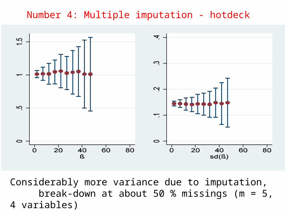
Considerably more variance due to imputation, break-down at about 50 % missings (m = 5, 4 variables)

Number 4: Multiple imputation - hotdeck

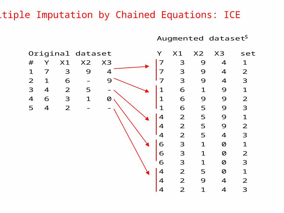
Multiple Imputation by Chained Equations: ICE

Augmented dataset

Original dataset Y X1 X2 X3 set

# Y X1 X2 X3 7 3 9 4 1

1 7 3 9 4 7 3 9 4 2

2 1 6 - 9 7 3 9 4 3

3 4 2 5 - 1 6 1 9 1

4 6 3 1 0 1 6 9 9 2

5 4 2 - - 1 6 5 9 3

4 2 5 9 1

4 2 5 9 2

4 2 5 4 3

6 3 1 0 1

6 3 1 0 2

6 3 1 0 3

4 2 5 0 1

4 2 9 4 2

4 2 1 4 3

s

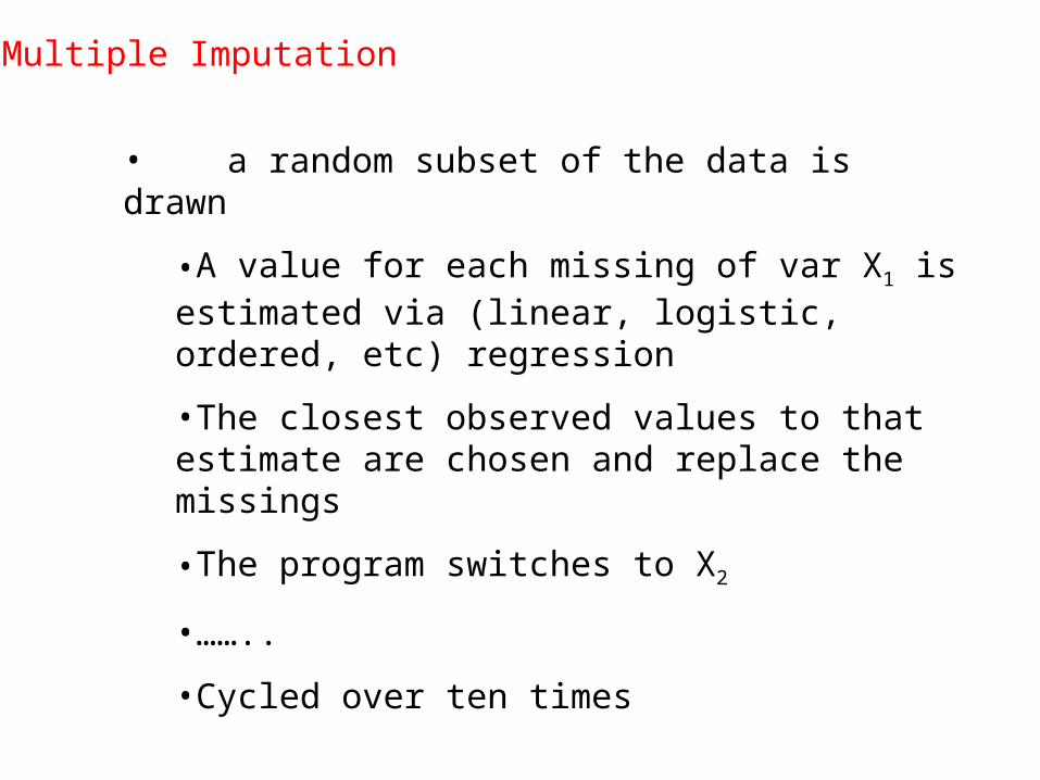
Multiple Imputation 

• a random subset of the data is drawn

•A value for each missing of var X1 is estimated via (linear, logistic, ordered, etc) regression

•The closest observed values to that estimate are chosen and replace the missings

•The program switches to X2

•……..

•Cycled over ten times

Finish when m datasets are created

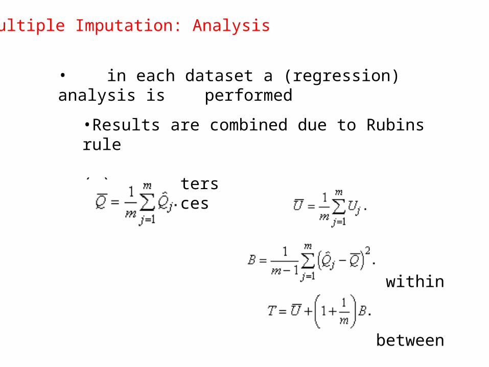
Multiple Imputation: Analysis 

• in each dataset a (regression) analysis is performed

•Results are combined due to Rubins rule

(a) parameters (b) variances

within

between

total

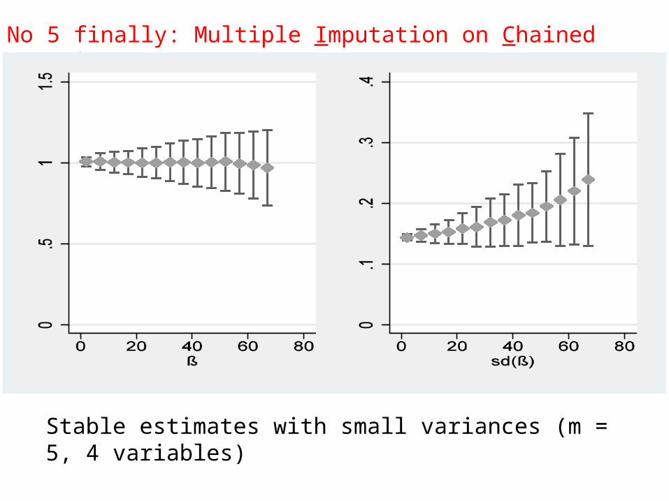
Stable estimates with small variances (m = 5, 4 variables)

No 5 finally: Multiple Imputation on Chained Equations - ICE

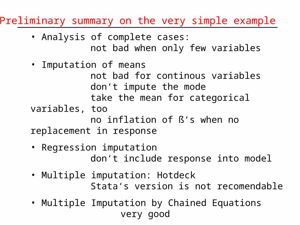
• Analysis of complete cases: not bad when only few variables

• Imputation of meansnot bad for continous variables don‘t impute the mode

take the mean for categorical variables, too

no inflation of ß‘s when no replacement in response

• Regression imputationdon‘t include response into model

• Multiple imputation: HotdeckStata‘s version is not recomendable

• Multiple Imputation by Chained Equationsvery good

Let‘s have a look onto a not so simple example

Preliminary summary on the very simple example

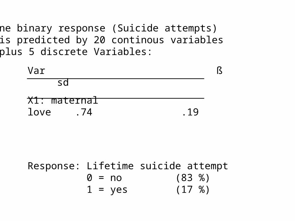
Var ß sd

X1: maternal love .74 .19

Response: Lifetime suicide attempt 0 = no (83 %)

1 = yes (17 %)

N = 505

One binary response (Suicide attempts) is predicted by 20 continous variables plus 5 discrete Variables:

-10

12

0 20 40 60ß = .76, n = 200

Percent missing in x

ICE estimate for beta,

4 variables in the model, CMAR

ICE estimate for beta,

4 variables in the model , CMAR

-10

12

0 20 40 60ß = .74, n = 100

Percent missing in x

ICE estimate for beta,

4 variables in the model , CMAR

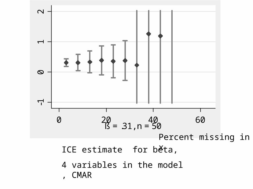
-10

12

0 20 40 60ß = .31, n = 50

Percent missing in x

ICE estimate for beta,

11 variables in the model , CMAR

-10

12

0 20 40 60ß = .74, n = 100

Percent missing in x

ICE estimate for beta,

25 variables in the model , CMAR

-10

12

0 20 40 60ß = .74, n = 100

Percent missing in x

The same done with MICE in R

-10

12

0 20 40 60ß = .74, n = 100

Percent missing in x

estimate for beta,

11 variables in the model , CMAR

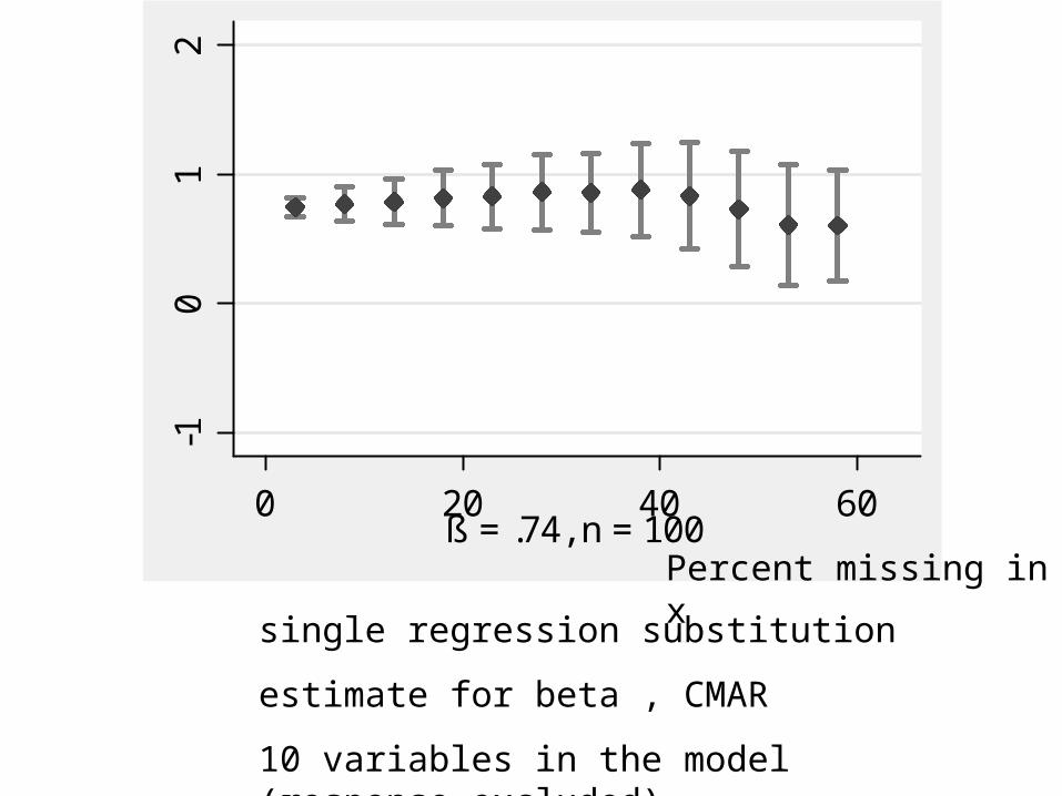
single regression substitution

estimate for beta , CMAR

10 variables in the model (response excluded)

-10

12

0 20 40 60ß = .74, n = 100

Percent missing in x

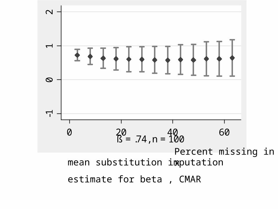
mean substitution imputation

estimate for beta , CMAR

-10

12

0 20 40 60ß = .74, n = 100

Percent missing in x

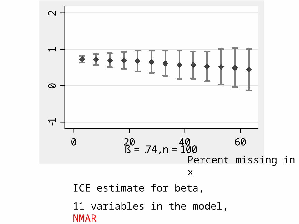
ICE estimate for beta,

11 variables in the model, NMAR

-10

12

0 20 40 60ß = .74, n = 100

Percent missing in x

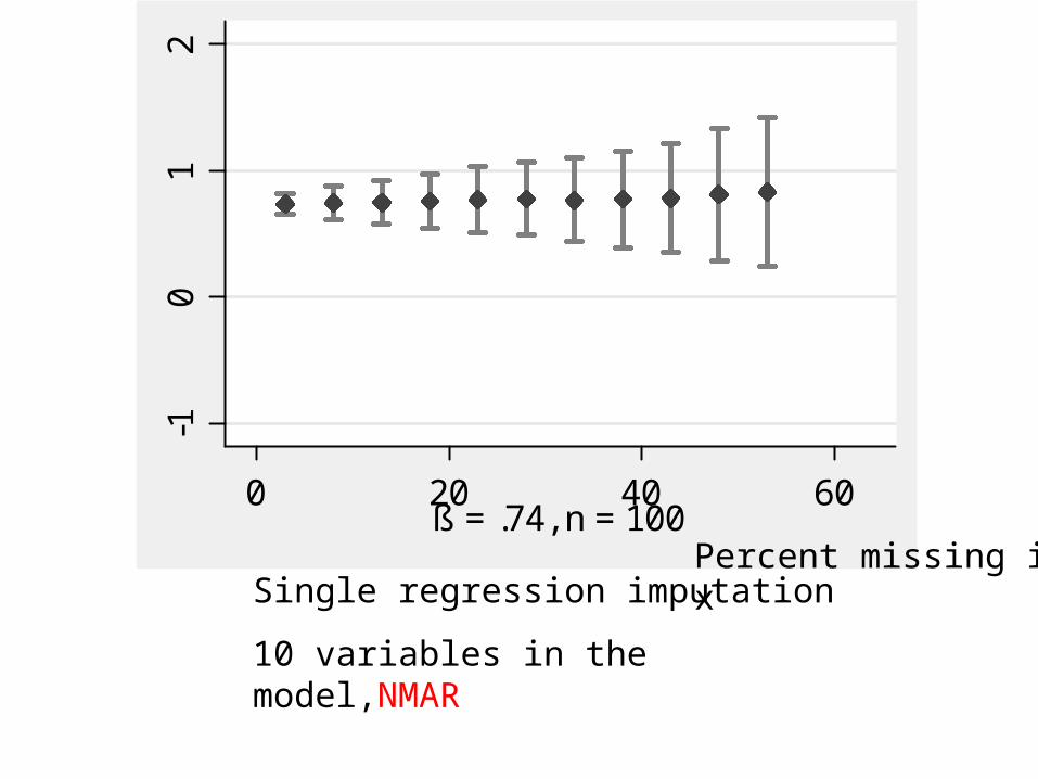
Single regression imputation

10 variables in the model,NMAR

-10

12

0 20 40 60ß = .74, n = 100

Percent missing in x

All non-linear effects are downward biased by any method. The example shows an interaction coefficient estimated with ICE, 11 variables in the model, CMAR

-10

12

0 20 40 60ß = .71, n = 100

Percent missing in x

Summary

- In large samples we can substitute considerable higher proportions of missings than in small ones.

- Multiple imputation with ICE performs well in all situations (as far as we examined)

- Having more variables in the imputation model leads to better estimates, i.e.smaller sd’s.

- With binary responses, ICE may report extreme sd’s when the number of variables grows high, or the number of cases low. Then we have gone too far.

- Single regression imputation performs quite well under certain conditions

- Non-linear effects get lost with all methods