Multilevel/Mixed Models and Longitudinal Analysis Using...

Alan C. Acock University Distinguished Professor of Family Studies &

Knudson Chair for Family Research & Policy Oregon State University

College of Health and Human Sciences Summer Workshop Series

July 2010

Multilevel/Mixed Models and Longitudinal Analysis Using Stata

A multilevel application Using Stata

What’s in a name?   A multilevel model simply has repeated measures on

something.

Alan C. Acock, July, 2010 2

What about levels   Trajectory for school engagement between 10 and 15

  Level 1 is the level of school engagement measured each spring   Level 2 is the person   Level 3 could be the school

  What Questions are we asking?  What is the overall trajectory defined by an intercept and a

slope (fixed effect)


Shortest possible history   Stata 1.0 was released in 1985 on the mainframe

  Moved to PCs in 1986 and has never returned to mainframes.

  Today it has platforms for

 Windows

 Macs

 Multiple flavors of Unix

  32 bit and 64 bit


Why do they say Stata is so fast?   It puts everything in RAM. Most of Stata’s development has

occurred after RAM became fairly cheap. There is no hard disk light flashing when you run Stata. RAM is 100 times as fast as a hard disk.

  Downside is there is a limit on how many variables you can analyze.  The IC version has a limit of 2,047 variables  The full versions have a limit of 32,767 variables


Learning Stata: Stata Press   For your Statistics Library:

  Acock, A.C. (2010). A gentle introduction to Stata, 3rd ed. Very introductory   Cameron, A. C., & Pravin, K. T. (2010). Microeconomics using Stata, revised

Edition. If you have/want and econometrics backgrounds   Long, J. S., & Freese, J. (2006). Regression Models for Categorical

Dependent Variables Using Stata, 2nd ed. Greatly advances what is usually done with categorical and count outcomes

  Rabe-Hesketh, S., & Skrondal, A. (2008). Multilevel and Longitudinal Modeling Using Stata, 2nd ed. This is the basis for today’s workshop

  Mitchel, M. N. (2008). A Visual Guide to Stata Graphics, 2nd ed. Small pictures of hundreds of graphs and the code that produces them


Learning Stata: Stata Press   For your Project/Data Management Library

  Long, J.S. (2009). The Workflow of Data Analysis Using Stata. Critical reading for anybody starting or managing a project, even if they don’t use Stata

 Mitchel, M. N. (2010). Data Management Using Stata: A Practical Handbook. All the tips and tricks for managing data


Learning Stata: StataCorp   Help. Run help commandname. Try help regress!

  At bottom of explanation you see a link to the manual   Manual examples start with simple and get more complicated   All data for them is online

  Online Manual has 8,000 pages in PDF files   Technical support: [email protected]   Within Stata run the command findit topic. Try findit reverse code. Install revrs.

  When you know a command, findit fre.ado!


Learning Stata: StataCorp   Strong Menu system

  Easier to use than the one for SAS   Somewhat harder to navigate than the one for SPSS

  Great way to learn all the features of a command   Run the menu for regress and explore the options

  Menu creates a command that you should save to a do-file (explained in a minute)


Learning Stata: UCLA Stata Portal   UCLA has the most comprehensive support for Stata at

http://statcomp.ats.ucla.edu/stata/   They say this is not actively being maintained and give a

link, but I find it is still useful.   The first line is “Resources to help you learn Stata . . . “   Tidbit of the week. Michael Mitchell has a weekly email

that has a neat feature of Stata.   Subscribe or check past tidbits   http://www.michaelnormanmitchell.com/


Learning Stata: UCLA Stata Portal


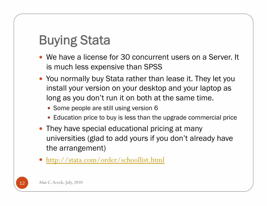
Buying Stata   We have a license for 30 concurrent users on a Server. It

is much less expensive than SPSS   You normally buy Stata rather than lease it. They let you

install your version on your desktop and your laptop as long as you don’t run it on both at the same time.   Some people are still using version 6   Education price to buy is less than the upgrade commercial price

  They have special educational pricing at many universities (glad to add yours if you don’t already have the arrangement)

  http://stata.com/order/schoollist.html


Buying Stata: Educational Plan


How Popular is Stata


  There are fields where it is very popular and other fields where it has yet to gain a strong following

  It has exceptional strength in econometrics and biostatistics   Its total sales compared to SAS and SPSS are still fairly small

and they dominate the corporate world   Stata is gaining ground in scholarly fields   Robert Muenchen did a Google Scholar plot of data analysis

software   For many routine studies this is not reported, mostly when

statistically sophisticated models are estimated   For 2010 he only has the first six months

How Popular is Stata


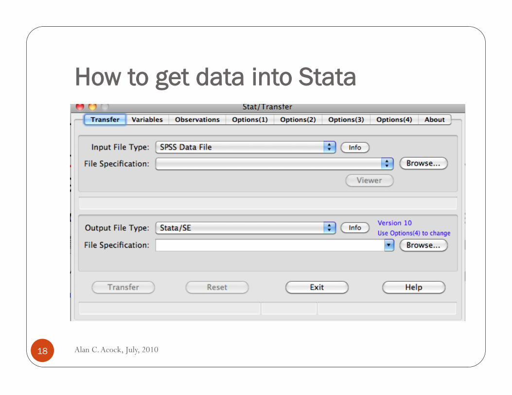
How to get data into Stata   If you want to use another program to manage your data,

buying StatTransfer is a good idea.   Stata has it for $69   StatTransfer has it for $179, but has a special student price of

$59. Updates are $95 ($39 for students).   Updates are a problem since some packages change their format

and an older version of StatTransfer won’t work

  SPSS will save files as a Stata Dataset, but doesn’t do a great job of it.   Compress after reading it into Stata


How to get data into Stata


Stata Conventions   Keep in mind that there are two files. One on your hard

disk and one active in memory (RAM).   Changes you make in the make in the active dataset must be saved   If you mess something up terribly, just close Stata without saving the

dataset.

  Stata documentation precedes a Stata command with a dot (.).   . summarize v1 – v500!

  Stata is case sensitive: SES ≠ Ses ≠ ses/   NORMALLY MAKE ALL VARIABLES LOWER CASE—No need to remember case   Rare exception might be where you generate an interaction such as genderXses!  If you capitalize this way you need to always do it


Stata Conventions   Stata updates frequently. Good to enter query update   Command end—a command ≠a line

  SAS uses a semi-colon   SPSS uses a period to end a command

  Stata uses a carriage return—   most commands are very short and fit easily on one actual line.   If more than one line is needed you enter a space and three slashes ///   Stata reads the /// as telling it to ignore the carriage return


Stata Interface


Introductory Statistics Using Stata   Stata has a strict format for virtually all statistical commands

  Type a little get a little

 The basic commands gives you what you want in most cases

 You can have a comma at the end of the command and then have options

 There are post estimation commands that give you specialized results


Introductory Statistics Using Stata   Format

 Command name variable list restrictions, options

  If there is a dependent variable, it is first on your variable list

 Here is an example:

. regress y x1 x2 x3, beta!


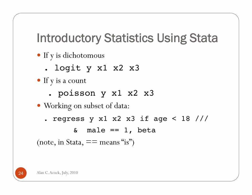
Introductory Statistics Using Stata   If y is dichotomous

. logit y x1 x2 x3!  If y is a count . poisson y x1 x2 x3! Working on subset of data: !. regress y x1 x2 x3 if age < 18 /// !! ! & male == 1, beta!

(note, in Stata, == means “is”)


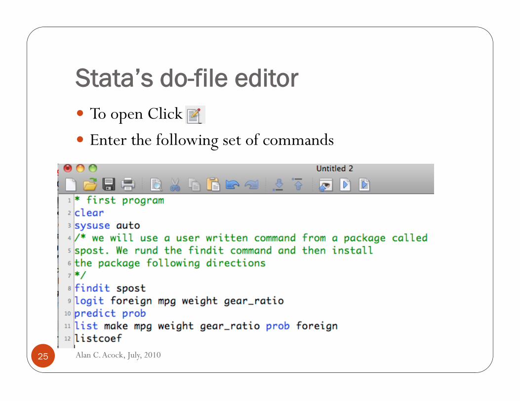
Stata’s do-file editor   To open Click   Enter the following set of commands


The Program   The clear is there to clear memory. So we can add a

new dataset.   The sysuse auto opens a dataset that is part of The

Stata Insulation   To run a single command or a subset, highlight and click the

top-right icon,   Don’t highlight and click the icon to run the entire program


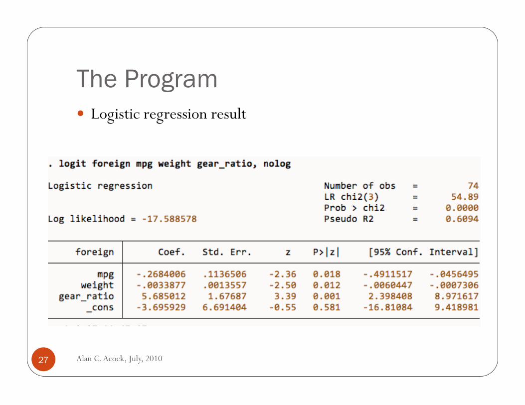
The Program   Logistic regression result


The Program   predict prob will predict the probability for each

case, i.e., probability foreign


The Program   Listcoef gives more information


The Program •  Since weight has a standard deviation of 777 and gear-ratio

has a standard deviation of .46, a one unit change in each of them has a very different meaning

•  The e^bStdX is the odds ratio for a one standard deviation change in the predictor and this makes more sense than a one unit change when predictors are on different scales


Reshaping Datasets •  Most datasets are wide

•  Each person has one record •  If there are repeated measures these might be labeled

•  weight1 weight2 weight3, etc.

•  For longitudinal or multilevel analysis we need data to be long •  Each wave has one record •  There would be three records for each case, first with wave 1

data, second with wave 2 data, etc.


Reshaping Datasets . webuse reshape1, clear!. list!


Reshaping Datasets •  Wide—Each person has 3 waves of data about their income •  Income variables end with a sequence of numbers, 80, 81, 82

•  You might use 1, 2, 3, 4, etc. •  Ignore the ue80, ue81, and ue82!

•  Long—We want three records for each case


Reshaping Datasets • The command !. reshape long inc ue, i(id) j(year)!• inc and ue are the repeated measures •  The i(id) tells Stata what the identification variable is for

each case •  The j(year) creates a new variable that tells us the year,

80, 81, 82 •  Could use j(wave) for longitudinal data •  Could use j(member) for multilevel data where there were j

members of each group


Reshaping Datasets


Reshaping Datasets   At this point we can go back to wide !. reshape wide!  And then back to long !. reshape long!  This switching is great when we need to do something that

requires a wide or long layout of the data.


Multilevel/Mixed Models and Longitudinal Analysis Using...

Documents

Transcript of Multilevel/Mixed Models and Longitudinal Analysis Using...