Introduction to Growth Curves Using Statapeople.oregonstate.edu/~acock/growth/2010 Mplus...
34
7/12/10 1 Alan C. Acock University Distinguished Professor of Family Studies & Knudson Chair for Family Research & Policy Oregon State University College of Health and Human Sciences Summer Workshop Series July 2010 Multilevel/Mixed Models and Longitudinal Analysis Using Stata Introduction to Growth Curves Using Stata
Transcript of Introduction to Growth Curves Using Statapeople.oregonstate.edu/~acock/growth/2010 Mplus...
7/12/10
1
Alan C. Acock University Distinguished Professor of Family Studies &
Knudson Chair for Family Research & Policy Oregon State University
College of Health and Human Sciences Summer Workshop Series
July 2010
Multilevel/Mixed Models and Longitudinal Analysis Using Stata
Introduction to Growth Curves Using Stata
7/12/10
2
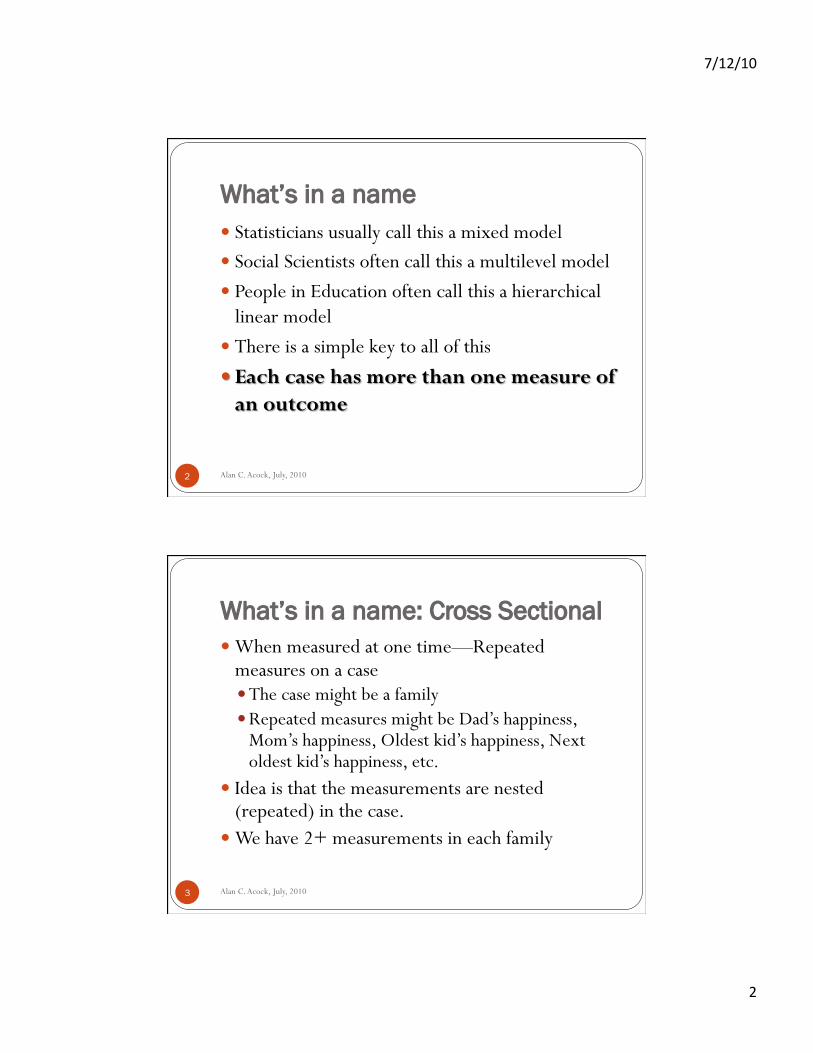
What’s in a name
Alan C. Acock, July, 2010 2
What’s in a name: Cross Sectional When measured at one time—Repeated
measures on a case The case might be a family Repeated measures might be Dad’s happiness,
Mom’s happiness, Oldest kid’s happiness, Next oldest kid’s happiness, etc.
Idea is that the measurements are nested (repeated) in the case.
We have 2+ measurements in each family
Alan C. Acock, July, 2010 3
7/12/10
3
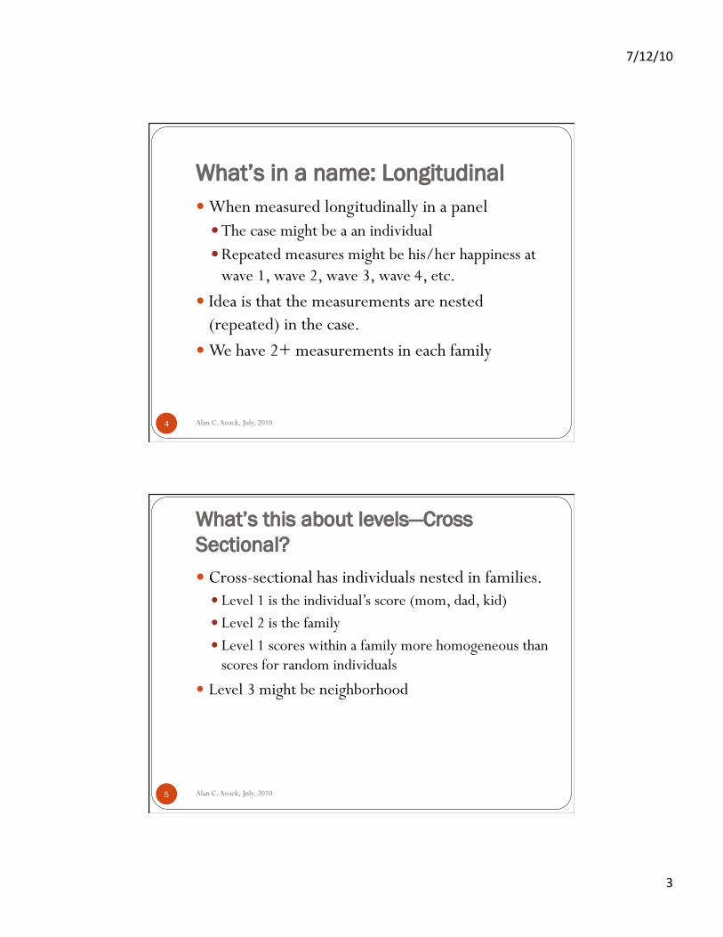
What’s in a name: Longitudinal When measured longitudinally in a panel The case might be a an individual Repeated measures might be his/her happiness at
wave 1, wave 2, wave 3, wave 4, etc. Idea is that the measurements are nested
(repeated) in the case. We have 2+ measurements in each family
Alan C. Acock, July, 2010 4
What’s this about levels—Cross Sectional? Cross-sectional has individuals nested in families.
Level 1 is the individual’s score (mom, dad, kid) Level 2 is the family Level 1 scores within a family more homogeneous than
scores for random individuals
Level 3 might be neighborhood
Alan C. Acock, July, 2010 5
7/12/10
4
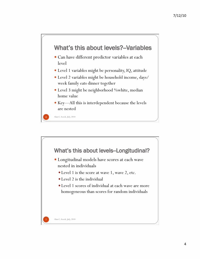
What’s this about levels?--Variables Can have different predictor variables at each
level Level 1 variables might be personality, IQ, attitude Level 2 variables might be household income, days/
week family eats dinner together
Level 3 might be neighborhood %white, median home value
Key—All this is interdependent because the levels are nested
Alan C. Acock, July, 2010 6
What’s this about levels--Longitudinal? Longitudinal models have scores at each wave
nested in individuals Level 1 is the score at wave 1, wave 2, etc. Level 2 is the individual Level 1 scores of individual at each wave are more
homogeneous than scores for random individuals
Alan C. Acock, July, 2010 7
7/12/10
5
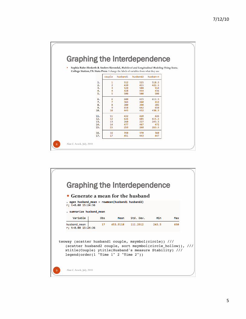
Graphing the Interdependence Sophia Rabe-Hesketh & Anders Skrondal, Multilevel and Longitudinal Modeling Using Stata.
College Station, TX: Stata Press. I change the labels of variables from what they use
Alan C. Acock, July, 2010 8
Graphing the Interdependence Generate a mean for the husband
Alan C. Acock, July, 2010 9
twoway (scatter husband1 couple, msymbol(circle)) ///! (scatter husband2 couple, sort msymbol(circle_hollow)), ///! xtitle(Couple) ytitle(Husband's measure Stability) ///! legend(order(1 "Time 1" 2 "Time 2")) !
7/12/10
6
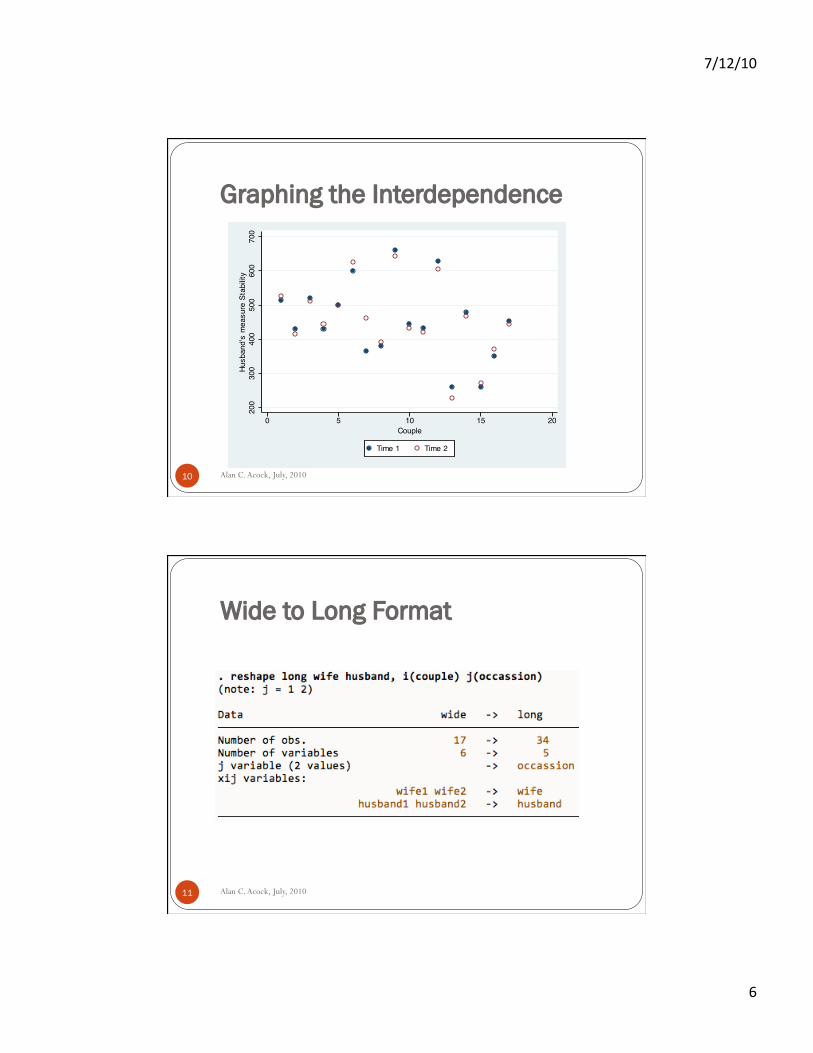
Graphing the Interdependence
Alan C. Acock, July, 2010 10
200
300
400
500
600
700
Husb
and'
s m
easu
re S
tabi
lity
0 5 10 15 20Couple
Time 1 Time 2
Wide to Long Format
Alan C. Acock, July, 2010 11
7/12/10
7
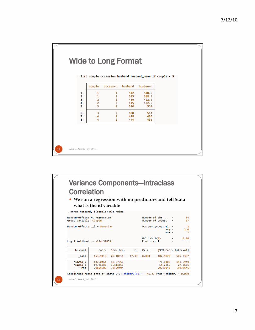
Wide to Long Format
Alan C. Acock, July, 2010 12
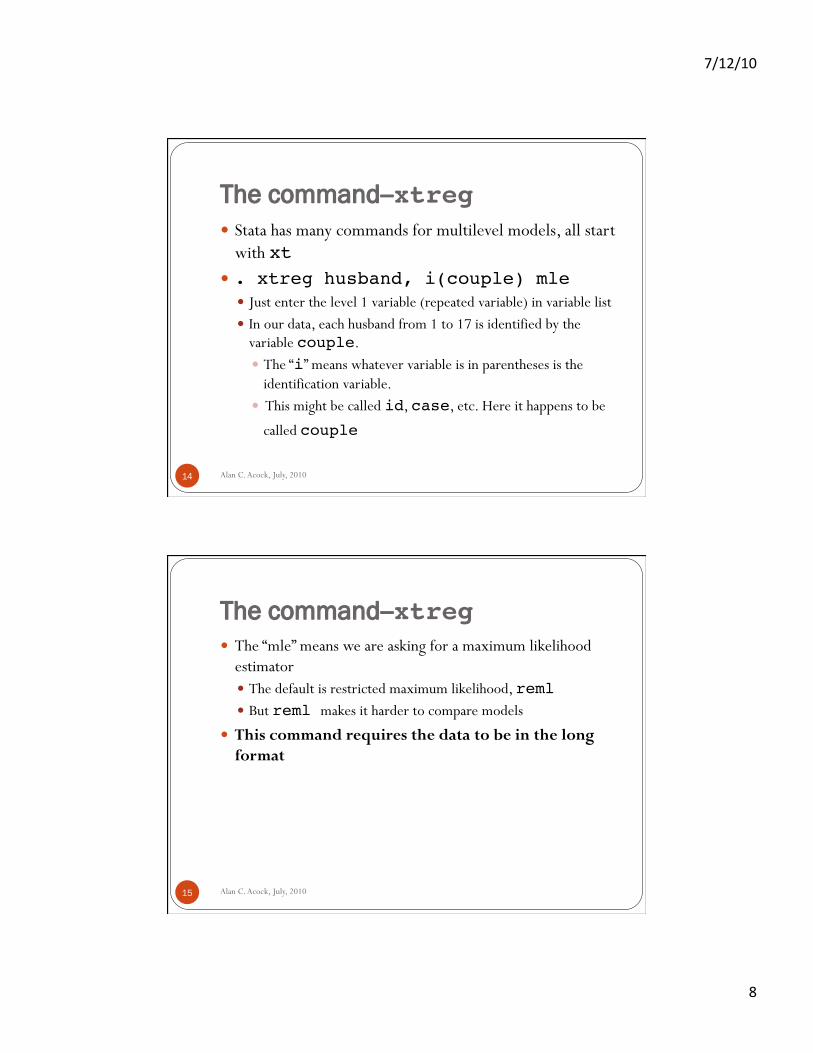
Variance Components—Intraclass Correlation We run a regression with no predictors and tell Stata
what is the id variable
Alan C. Acock, July, 2010 13
7/12/10
8
The command--xtreg! Stata has many commands for multilevel models, all start
with xt! . xtreg husband, i(couple) mle!
Just enter the level 1 variable (repeated variable) in variable list In our data, each husband from 1 to 17 is identified by the
variable couple. The “i” means whatever variable is in parentheses is the
identification variable. This might be called id, case, etc. Here it happens to be
called couple
Alan C. Acock, July, 2010 14
The command--xtreg! The “mle” means we are asking for a maximum likelihood
estimator The default is restricted maximum likelihood, reml ! But reml makes it harder to compare models
This command requires the data to be in the long format
Alan C. Acock, July, 2010 15
7/12/10
9
The xtreg Result
Alan C. Acock, July, 2010 16
The xtreg Result
Alan C. Acock, July, 2010 17
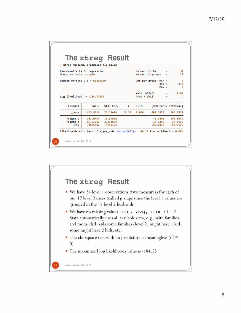
We have 34 level 1 observations (two measures) for each of our 17 level 2 cases (called groups since the level 1 values are grouped in the 17 level 2 husbands
We have no missing values: min, avg, max all = 2. Stata automatically uses all available data, e.g., with families and mom, dad, kids some families (level 2) might have 1 kid, some might have 2 kids, etc.
The chi-square test with no predictors is meaningless (df = 0)
The maximized log likelihoods value is -184.58
7/12/10
10
The xtreg Result
Alan C. Acock, July, 2010 18
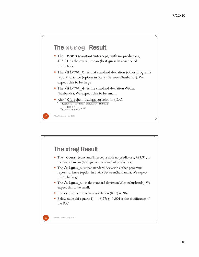
The _cons (constant/intercept) with no predictors, 453.91, is the overall mean (best guess in absence of predictors)
The /sigma_u is that standard deviation (other programs report variance (option in Stata) Between(husbands). We expect this to be large
The /sigma_e is the standard deviation Within(husbands). We expect this to be small.
Rho (ρ) is the intraclass correlation (ICC) ICC =
Var(Between)Var(Between) +Var(Within
=SD(Between)2
SD(Between)2 + SD(Within)2
=107.04642
107.04642 +19.910832= .967
The xtreg Result
Alan C. Acock, July, 2010 19
The _cons (constant/intercept) with no predictors, 453.91, is the overall mean (best guess in absence of predictors)
The /sigma_u is that standard deviation (other programs report variance (option in Stata) Between(husbands). We expect this to be large
The /sigma_e is the standard deviation Within(husbands). We expect this to be small.
Rho (ρ) is the intraclass correlation (ICC) is .967 Below table chi-square(1) = 46.27; p < .001 is the significance of
the ICC
7/12/10
11
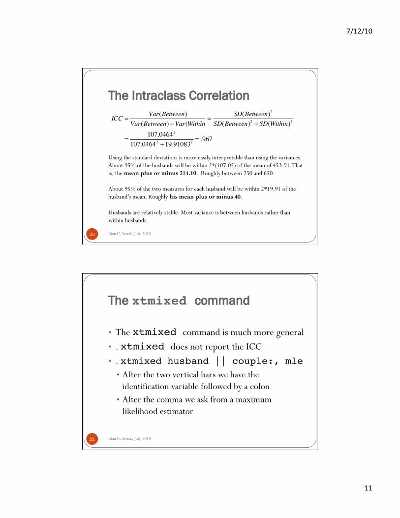
The Intraclass Correlation
Alan C. Acock, July, 2010 20
ICC =Var(Between)
Var(Between) +Var(Within=
SD(Between)2
SD(Between)2 + SD(Within)2
=107.04642
107.04642 +19.910832= .967
Using the standard deviations is more easily interpretable than using the variances. About 95% of the husbands will be within 2*(107.05) of the mean of 453.91. That is, the mean plus or minus 214.10. Roughly between 250 and 650.
About 95% of the two measures for each husband will be within 2*19.91 of the husband’s mean. Roughly his mean plus or minus 40.
Husbands are relatively stable. Most variance is between husbands rather than within husbands.
The xtmixed command
• The xtmixed command is much more general • . xtmixed does not report the ICC • . xtmixed husband || couple:, mle!
• After the two vertical bars we have the identification variable followed by a colon
• After the comma we ask from a maximum likelihood estimator
Alan C. Acock, July, 2010 21
7/12/10
12
The xtmixed result
Alan C. Acock, July, 2010 22
The xtmixed result
Alan C. Acock, July, 2010 23
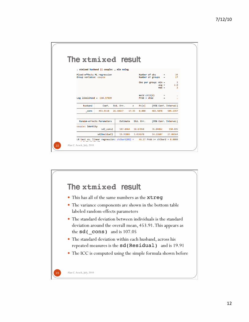
This has all of the same numbers as the xtreg! The variance components are shown in the bottom table
labeled random-effects parameters The standard deviation between individuals is the standard
deviation around the overall mean, 453.91. This appears as the sd(_cons) and is 107.05
The standard deviation within each husband, across his repeated measures is the sd(Residual) and is 19.91
The ICC is computed using the simple formula shown before
7/12/10
13
The xtmixed result—Conf. Intervals
Alan C. Acock, July, 2010 24
Both results show standard errors for the estimated standard deviations and 95% confidence intervals
These are somewhat problematic. The boundary space for a variance or standard deviation has a lower limit of zero
A similar problem occurs putting a confidence interval around a correlation coefficient since it can’t be below 0.
Stata adjusts for this by reporting an asymmetric confidence interval. A symmetrical C.I. for sd(Residual) would be
13.24-26.58
Graphic Representation of Variance Components
Alan C. Acock, July, 2010 25
H1
H2
ε11
ε21ζ1
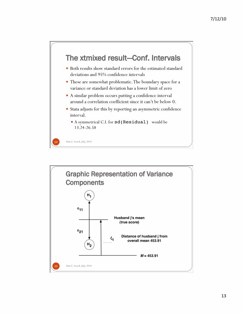
Husband j's mean (true score)
Distance of husband j from overall mean 453.91
M = 453.91
7/12/10
14
Graphic Representation of Variance Components
Alan C. Acock, July, 2010 26
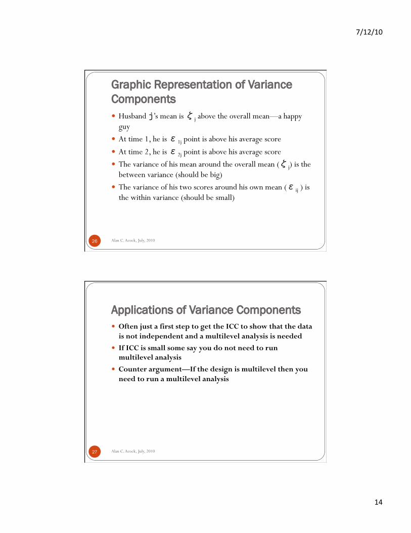
Husband j’s mean is ζj above the overall mean—a happy guy
At time 1, he is ε1j point is above his average score At time 2, he is ε2j point is above his average score The variance of his mean around the overall mean (ζj) is the
between variance (should be big) The variance of his two scores around his own mean (εij ) is
the within variance (should be small)
Applications of Variance Components Often just a first step to get the ICC to show that the data
is not independent and a multilevel analysis is needed If ICC is small some say you do not need to run
multilevel analysis Counter argument—If the design is multilevel then you
need to run a multilevel analysis
Alan C. Acock, July, 2010 27
7/12/10
15
Applications of Variance Components You don’t change the test you planned to do to get a
significant result If you set up a nonparametric test and it was not
significant, but then you noticed a few outliers, what would you do? Change to a t-test that is sensitive to outliers and might be significant Stay the course with your research design FDA expects drug companies to indicate what tests they will run
before they collect the data and does not allow them to try different tests till they find one is significant
If you set up a test using a two-tail assumption, can you change it to one-tail after seeing the result?
This is equivalent to not running a multilevel analysis after you see the ICC is small
Alan C. Acock, July, 2010 28
Applications of Variance Components Can use ICC and graph to see who is most similar Are wives more consistent than husbands? Are identical twins more similar than other twins? Are students in all female math classes more similar than
mixed math classes? Just compare the ICCs and possibly do a graph
Alan C. Acock, July, 2010 29
7/12/10
16
How many 2nd level groups are needed?
Alan C. Acock, July, 2010 30
• Here these are husbands • Could be families, organizations, classrooms, etc
• In a very real sense, these are your cases. • 30 to 50 seems reasonable • It is possible to do a power analysis
• If you had 5 classes, it would be like having 5 observations—a pretty small sample size
How many level 1 scores are needed?
Alan C. Acock, July, 2010 31
Here we only had 2, more would be very helpful Could be scores on members of a group—students
in a class (25-30), members of a family (3-6) Issue is getting a mean of these values to
represent some sense of a true score. Husband’s mean is his reference point Mean of 25 students in a class is the classes
reference point
7/12/10
17
Do-file
Alan C. Acock, July, 2010 32
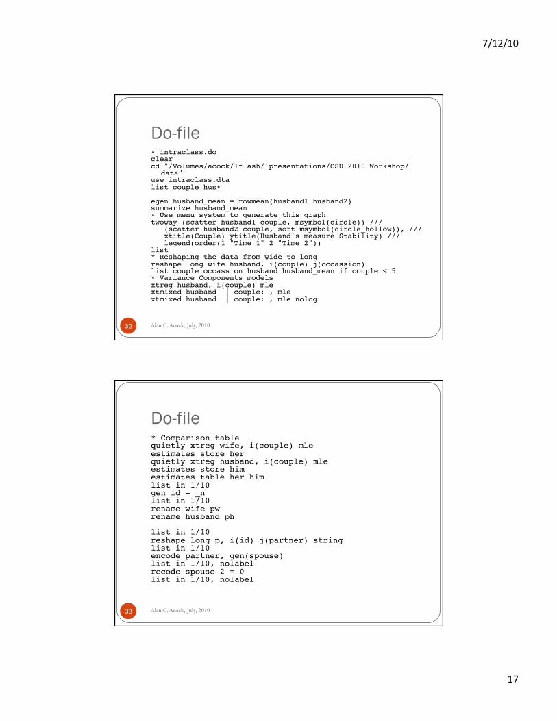
* intraclass.do!clear!cd "/Volumes/acock/1flash/1presentations/OSU 2010 Workshop/
data"!use intraclass.dta!list couple hus*!
egen husband_mean = rowmean(husband1 husband2)!summarize husband_mean!* Use menu system to generate this graph!twoway (scatter husband1 couple, msymbol(circle)) ///! (scatter husband2 couple, sort msymbol(circle_hollow)), ///! xtitle(Couple) ytitle(Husband's measure Stability) ///! legend(order(1 "Time 1" 2 "Time 2")) !list!* Reshaping the data from wide to long!reshape long wife husband, i(couple) j(occassion)!list couple occassion husband husband_mean if couple < 5!* Variance Components models!xtreg husband, i(couple) mle!xtmixed husband || couple: , mle!xtmixed husband || couple: , mle nolog!
Do-file
Alan C. Acock, July, 2010 33
* Comparison table!quietly xtreg wife, i(couple) mle!estimates store her!quietly xtreg husband, i(couple) mle!estimates store him!estimates table her him!list in 1/10!gen id = _n!list in 1/10!rename wife pw!rename husband ph!
list in 1/10!reshape long p, i(id) j(partner) string!list in 1/10!encode partner, gen(spouse)!list in 1/10, nolabel!recode spouse 2 = 0!list in 1/10, nolabel!
7/12/10
18
Do-file
Alan C. Acock, July, 2010 34
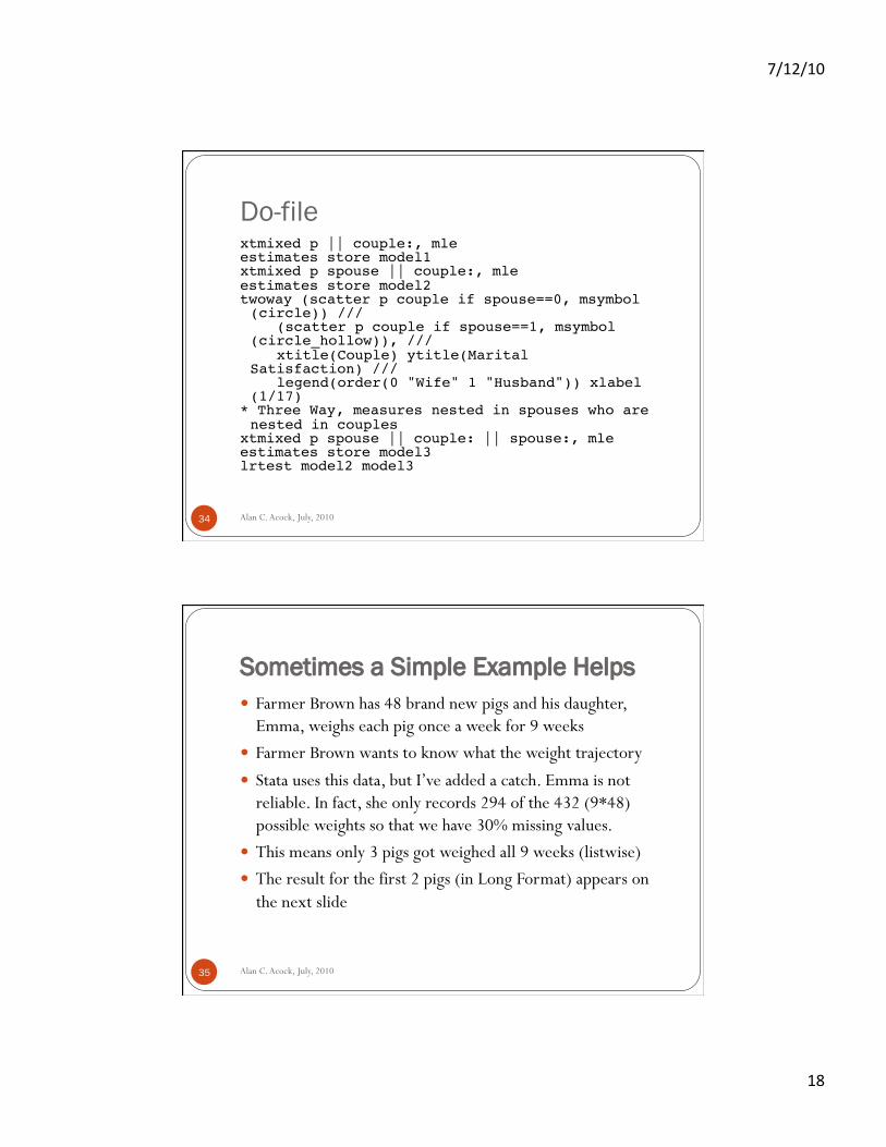
xtmixed p || couple:, mle!estimates store model1!xtmixed p spouse || couple:, mle!estimates store model2!twoway (scatter p couple if spouse==0, msymbol(circle)) ///!! (scatter p couple if spouse==1, msymbol(circle_hollow)), ///!! xtitle(Couple) ytitle(Marital Satisfaction) ///!! legend(order(0 "Wife" 1 "Husband")) xlabel(1/17)!
* Three Way, measures nested in spouses who are nested in couples!
xtmixed p spouse || couple: || spouse:, mle!estimates store model3!lrtest model2 model3!
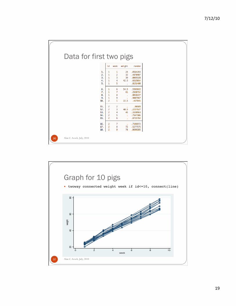
Sometimes a Simple Example Helps Farmer Brown has 48 brand new pigs and his daughter,
Emma, weighs each pig once a week for 9 weeks Farmer Brown wants to know what the weight trajectory Stata uses this data, but I’ve added a catch. Emma is not
reliable. In fact, she only records 294 of the 432 (9*48) possible weights so that we have 30% missing values.
This means only 3 pigs got weighed all 9 weeks (listwise) The result for the first 2 pigs (in Long Format) appears on
the next slide
Alan C. Acock, July, 2010 35
7/12/10
19
Data for first two pigs
Alan C. Acock, July, 2010 36
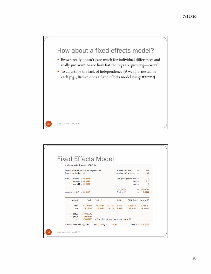
Graph for 10 pigs
Alan C. Acock, July, 2010 37
twoway connected weight week if id<=10, connect(line)!
2040
6080
weigh
t
0 2 4 6 8 10week
7/12/10
20
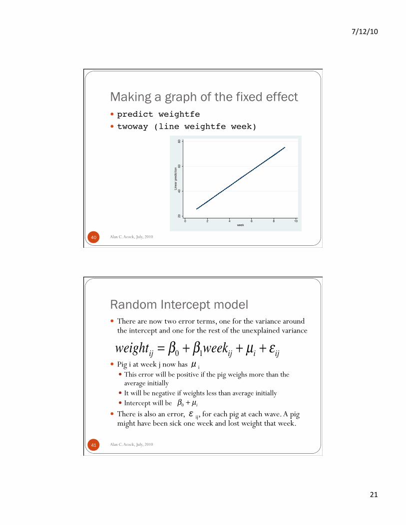
How about a fixed effects model?
Alan C. Acock, July, 2010 38
Brown really doesn’t care much for individual differences and really just want to see how fast the pigs are growing—overall
To adjust for the lack of independence (9 weights nested in each pig), Brown does a fixed effects model using xtreg!
Fixed Effects Model
Alan C. Acock, July, 2010 39
7/12/10
21
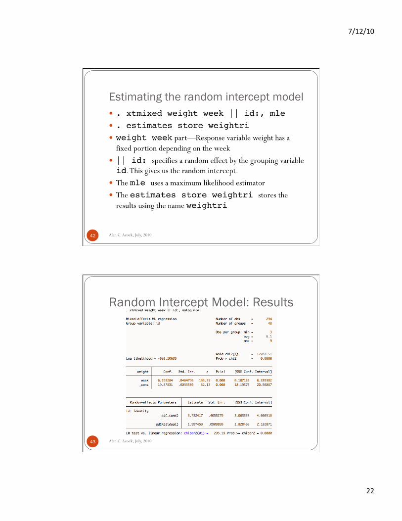
Making a graph of the fixed effect
Alan C. Acock, July, 2010 40
predict weightfe! twoway (line weightfe week)!
2040
6080
Line
ar p
redi
ctio
n
0 2 4 6 8 10week
Random Intercept model
Alan C. Acock, July, 2010 41
There are now two error terms, one for the variance around the intercept and one for the rest of the unexplained variance
Pig i at week j now has μi This error will be positive if the pig weighs more than the
average initially It will be negative if weights less than average initially Intercept will be
There is also an error, εij, for each pig at each wave. A pig might have been sick one week and lost weight that week.
weightij = β0 + β1weekij + µi + εij
β0 + µi
7/12/10
22
Estimating the random intercept model
Alan C. Acock, July, 2010 42
. xtmixed weight week || id:, mle! . estimates store weightri! weight week part—Response variable weight has a
fixed portion depending on the week || id: specifies a random effect by the grouping variable id. This gives us the random intercept.
The mle uses a maximum likelihood estimator The estimates store weightri stores the
results using the name weightri!
Random Intercept Model: Results
Alan C. Acock, July, 2010 43
7/12/10
23
Random Intercept Model: Interpretation
Alan C. Acock, July, 2010 44
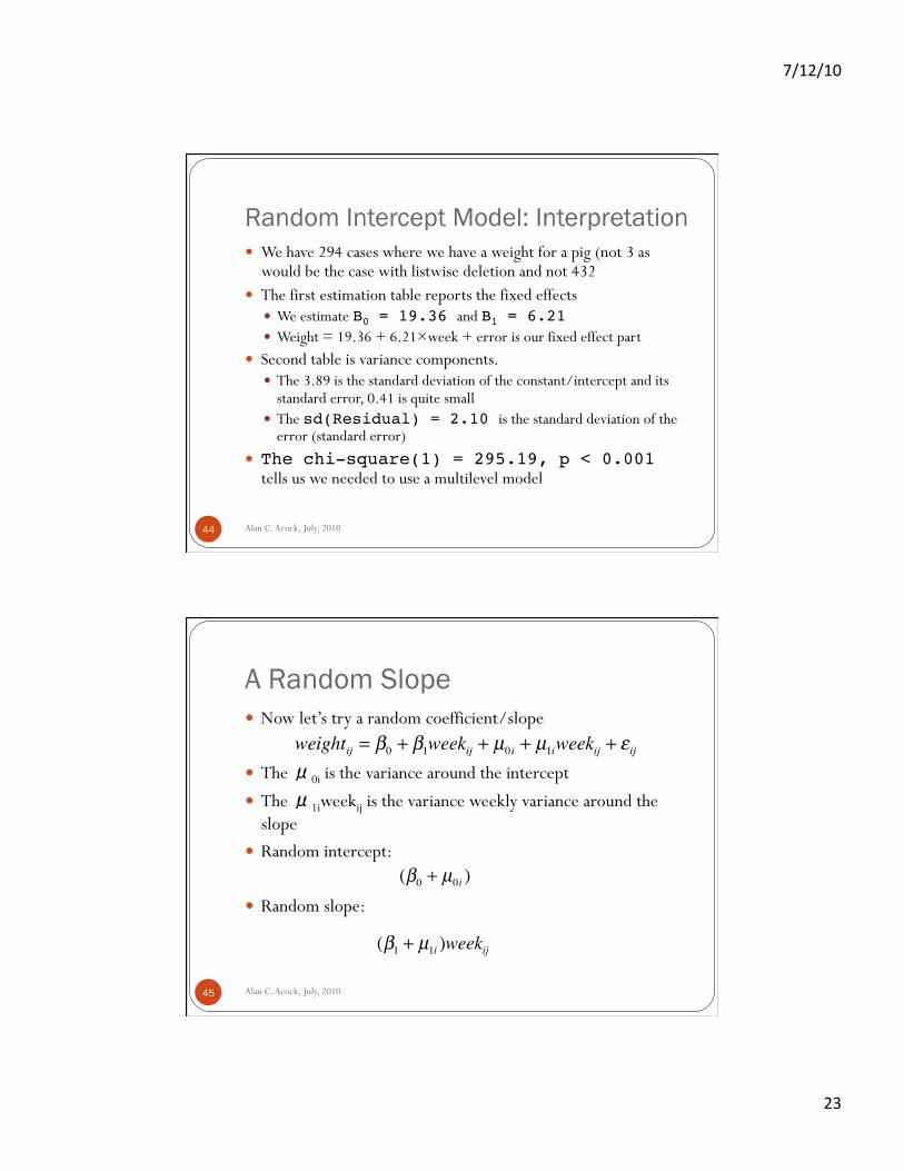
We have 294 cases where we have a weight for a pig (not 3 as would be the case with listwise deletion and not 432
The first estimation table reports the fixed effects We estimate B0 = 19.36 and B1 = 6.21! Weight = 19.36 + 6.21×week + error is our fixed effect part
Second table is variance components. The 3.89 is the standard deviation of the constant/intercept and its
standard error, 0.41 is quite small The sd(Residual) = 2.10 is the standard deviation of the
error (standard error) The chi-square(1) = 295.19, p < 0.001
tells us we needed to use a multilevel model
A Random Slope
Alan C. Acock, July, 2010 45
Now let’s try a random coefficient/slope
The μ0i is the variance around the intercept The μ1iweekij is the variance weekly variance around the
slope Random intercept:
Random slope:
weightij = β0 + β1weekij + µ0i + µ1iweekij + εij
(β0 + µ0i )
(β1 + µ1i )weekij
7/12/10
24
Covariance of Intercept & Slope
Alan C. Acock, July, 2010 46
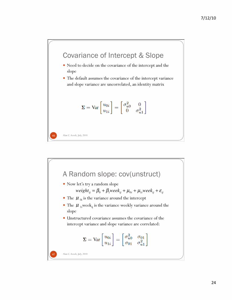
Need to decide on the covariance of the intercept and the slope
The default assumes the covariance of the intercept variance and slope variance are uncorrelated, an identity matrix
A Random slope: cov(unstruct)
Alan C. Acock, July, 2010 47
Now let’s try a random slope
The μ0i is the variance around the intercept The μ1iweekij is the variance weekly variance around the
slope Unstructured covariance assumes the covariance of the
intercept variance and slope variance are correlated:
weightij = β0 + β1weekij + µ0i + µ1iweekij + εij

7/12/10
25
Random Coefficients Model
Alan C. Acock, July, 2010 48
. xtmixed weight week || id: week, nolog mle cov(unstruct) var! . estimates store weightrc! . lrtest weightri weightrc!
The id: is the part of the command that gives us the random intercept
Any variable after the colon will have a random coefficient The variable week is allowed to have a different slope for each pig
since some grow faster than others The cov(unstruct) allows the random intercept and
random slope to be correlated Notice the var at the end means we are estimating variances
Alan C. Acock, July, 2010 49
7/12/10
26
School Engagement Example
Alan C. Acock, July, 2010 50
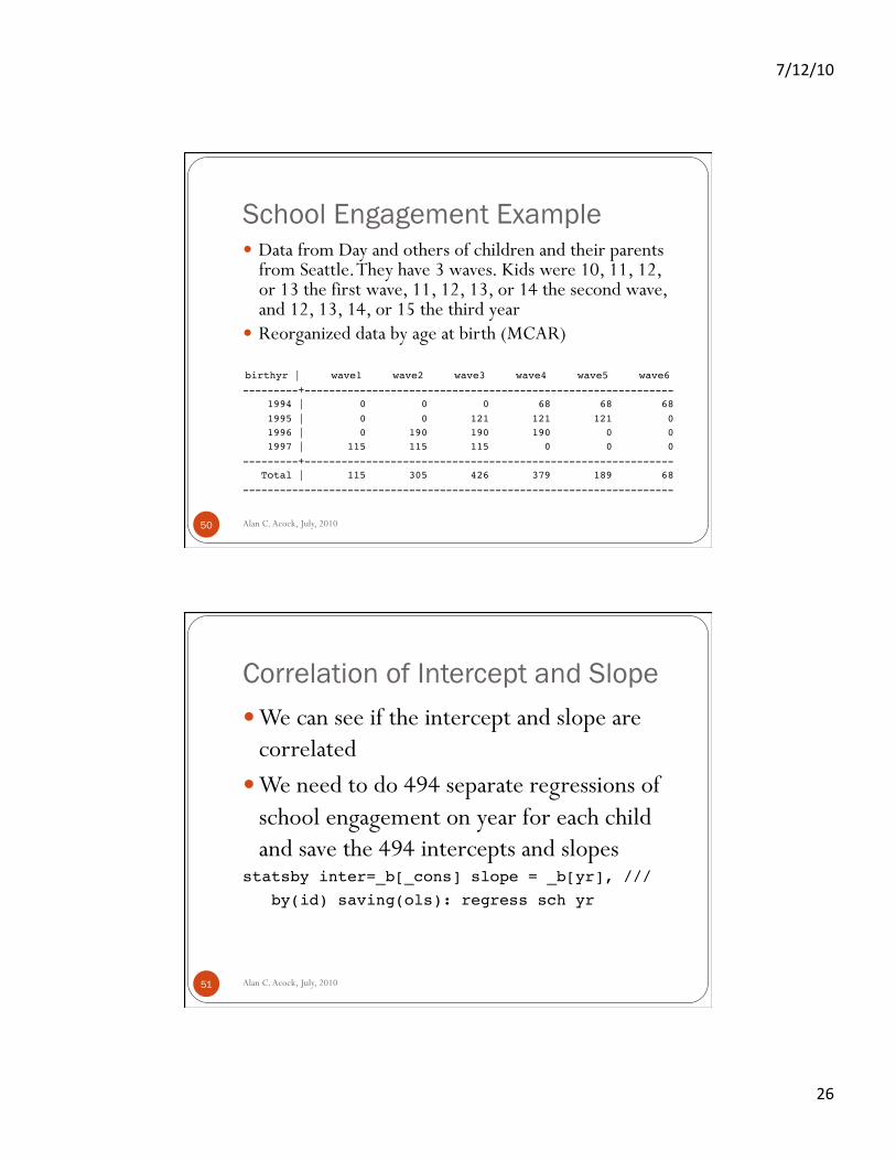
Data from Day and others of children and their parents from Seattle. They have 3 waves. Kids were 10, 11, 12, or 13 the first wave, 11, 12, 13, or 14 the second wave, and 12, 13, 14, or 15 the third year
Reorganized data by age at birth (MCAR)
birthyr | wave1 wave2 wave3 wave4 wave5 wave6!---------+------------------------------------------------------------! 1994 | 0 0 0 68 68 68! 1995 | 0 0 121 121 121 0! 1996 | 0 190 190 190 0 0! 1997 | 115 115 115 0 0 0!---------+------------------------------------------------------------! Total | 115 305 426 379 189 68!----------------------------------------------------------------------!
Correlation of Intercept and Slope
Alan C. Acock, July, 2010 51
We can see if the intercept and slope are correlated
We need to do 494 separate regressions of school engagement on year for each child and save the 494 intercepts and slopes
statsby inter=_b[_cons] slope = _b[yr], ///! by(id) saving(ols): regress sch yr!
7/12/10
27
Correlation of Intercept and Slope
Alan C. Acock, July, 2010 52
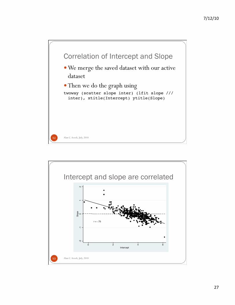
We merge the saved dataset with our active dataset
Then we do the graph using twoway (scatter slope inter) (lfit slope /// inter), xtitle(Intercept) ytitle(Slope)!
Intercept and slope are correlated
Alan C. Acock, July, 2010 53
r = -.73
-2-1
01
2Sl
ope
0 2 4 6Intercept
7/12/10
28
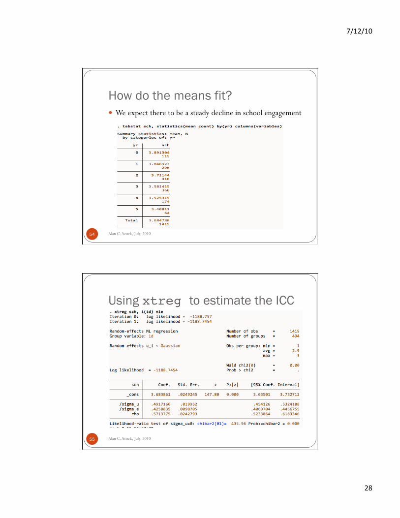
How do the means fit?
Alan C. Acock, July, 2010 54
We expect there to be a steady decline in school engagement
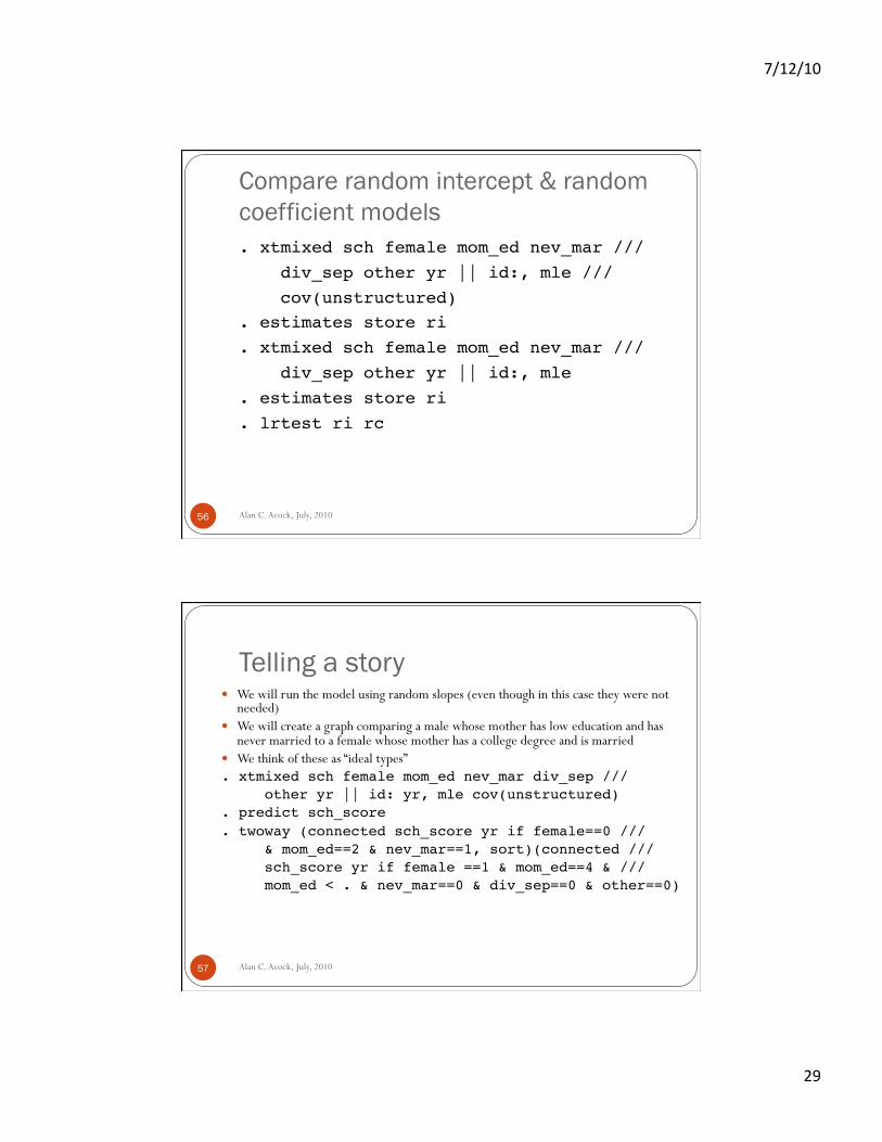
Using xtreg to estimate the ICC
Alan C. Acock, July, 2010 55
7/12/10
29
Compare random intercept & random coefficient models
Alan C. Acock, July, 2010 56
. xtmixed sch female mom_ed nev_mar ///! div_sep other yr || id:, mle ///! cov(unstructured)!. estimates store ri!. xtmixed sch female mom_ed nev_mar /// ! div_sep other yr || id:, mle!. estimates store ri!. lrtest ri rc!
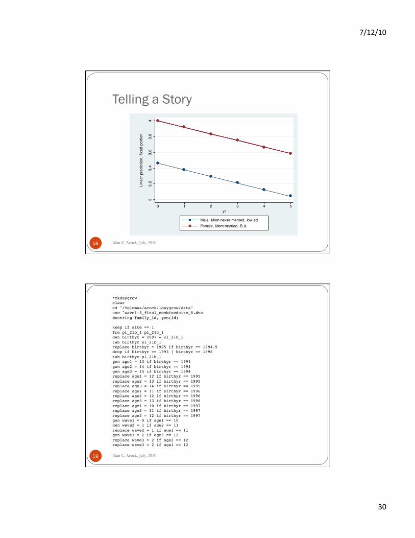
Telling a story
Alan C. Acock, July, 2010 57
We will run the model using random slopes (even though in this case they were not needed)
We will create a graph comparing a male whose mother has low education and has never married to a female whose mother has a college degree and is married
We think of these as “ideal types” . xtmixed sch female mom_ed nev_mar div_sep ///! other yr || id: yr, mle cov(unstructured)!. predict sch_score!. twoway (connected sch_score yr if female==0 ///! & mom_ed==2 & nev_mar==1, sort)(connected ///! sch_score yr if female ==1 & mom_ed==4 & ///! mom_ed < . & nev_mar==0 & div_sep==0 & other==0)!
7/12/10
30
Telling a Story
Alan C. Acock, July, 2010 58
33.
23.
43.
63.
84
Line
ar p
redi
ctio
n, fi
xed
porti
on
0 1 2 3 4 5yr
Male, Mom never married, low edFemale, Mom married, B.A.
Alan C. Acock, July, 2010 59
*mkdaygrow!clear!cd "/Volumes/acock/1daygrow/data"!use "wave1-3_final_combinedsite_8.dta!destring family_id, gen(id)!
keep if site == 1!fre p1_21b_1 p1_21c_1!gen birthyr = 2007 - p1_21b_1!tab birthyr p1_21b_1!replace birthyr = 1995 if birthyr == 1994.5!drop if birthyr == 1993 | birthyr == 1998!tab birthyr p1_21b_1!gen age1 = 13 if birthyr == 1994!gen age2 = 14 if birthyr == 1994!gen age3 = 15 if birthyr == 1994!replace age1 = 12 if birthyr == 1995!replace age2 = 13 if birthyr == 1995!replace age3 = 14 if birthyr == 1995!replace age1 = 11 if birthyr == 1996!replace age2 = 12 if birthyr == 1996!replace age3 = 13 if birthyr == 1996!replace age1 = 10 if birthyr == 1997!replace age2 = 11 if birthyr == 1997!replace age3 = 12 if birthyr == 1997!gen wave1 = 0 if age1 == 10!gen wave2 = 1 if age2 == 11!replace wave2 = 1 if age1 == 11!gen wave3 = 2 if age3 == 12!replace wave3 = 2 if age2 == 12!replace wave3 = 2 if age1 == 12!
7/12/10
31
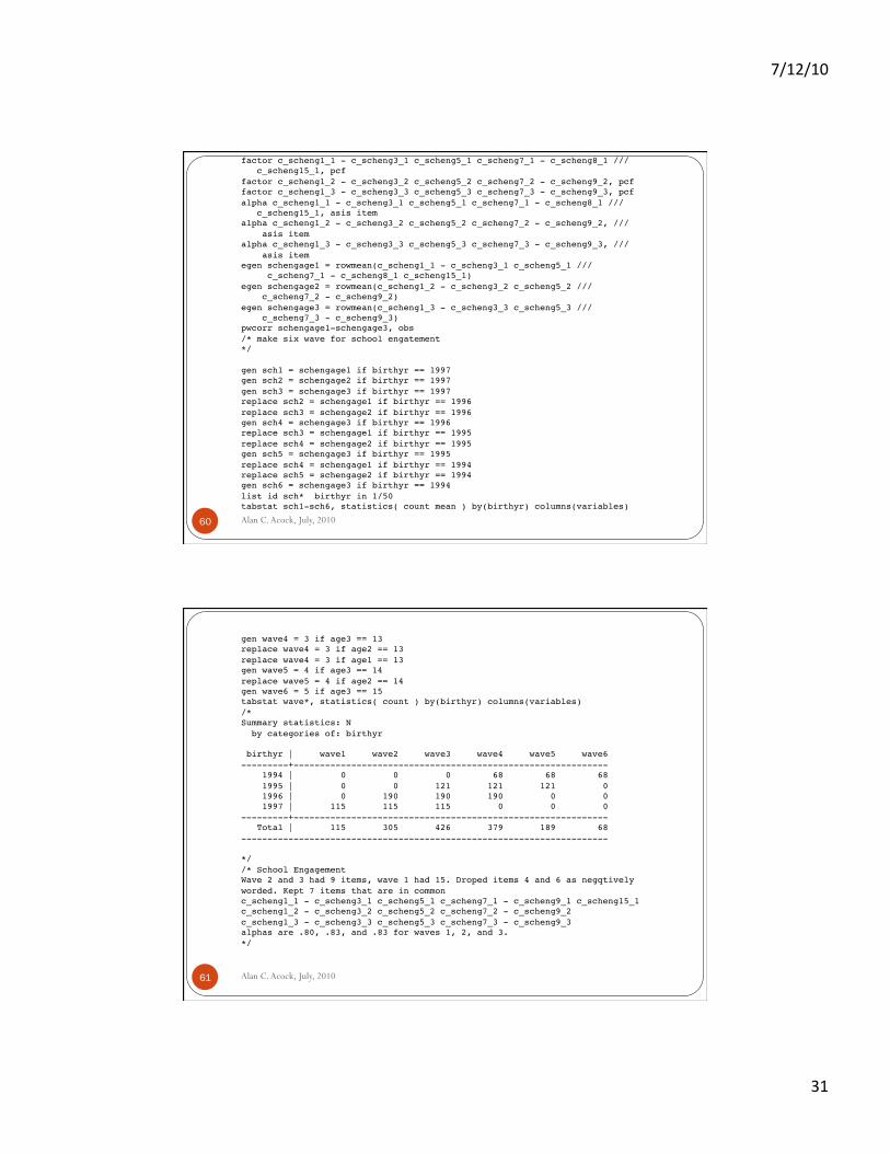
Alan C. Acock, July, 2010 60
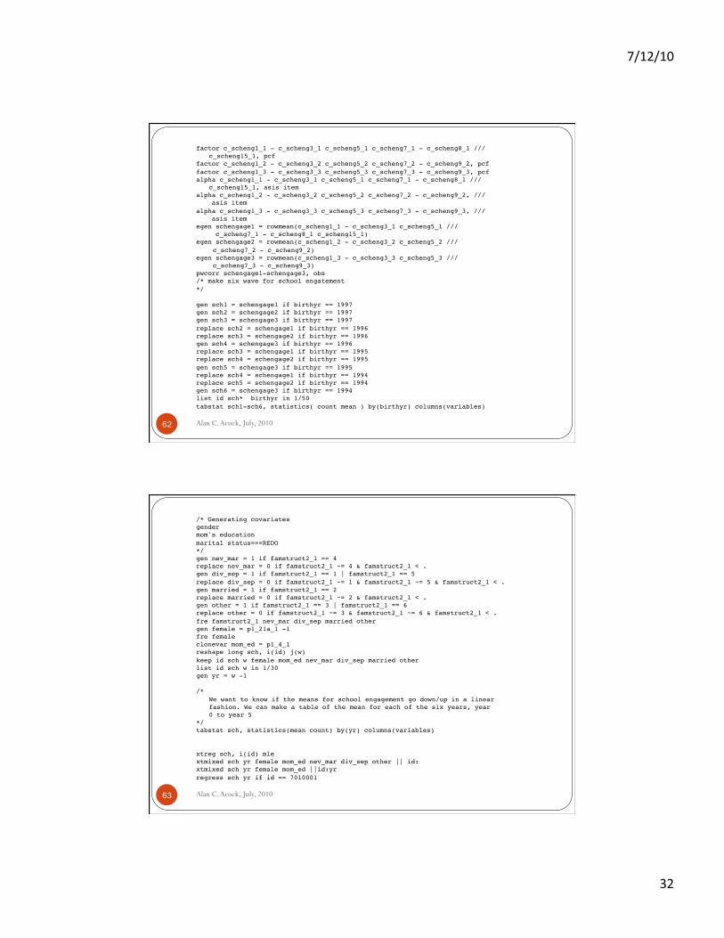
factor c_scheng1_1 - c_scheng3_1 c_scheng5_1 c_scheng7_1 - c_scheng8_1 ///!!c_scheng15_1, pcf!
factor c_scheng1_2 - c_scheng3_2 c_scheng5_2 c_scheng7_2 - c_scheng9_2, pcf!factor c_scheng1_3 - c_scheng3_3 c_scheng5_3 c_scheng7_3 - c_scheng9_3, pcf!alpha c_scheng1_1 - c_scheng3_1 c_scheng5_1 c_scheng7_1 - c_scheng8_1 ///!!c_scheng15_1, asis item!
alpha c_scheng1_2 - c_scheng3_2 c_scheng5_2 c_scheng7_2 - c_scheng9_2, ///! asis item!alpha c_scheng1_3 - c_scheng3_3 c_scheng5_3 c_scheng7_3 - c_scheng9_3, ///! asis item!egen schengage1 = rowmean(c_scheng1_1 - c_scheng3_1 c_scheng5_1 ///! c_scheng7_1 - c_scheng8_1 c_scheng15_1)!egen schengage2 = rowmean(c_scheng1_2 - c_scheng3_2 c_scheng5_2 ///!! c_scheng7_2 - c_scheng9_2) !
egen schengage3 = rowmean(c_scheng1_3 - c_scheng3_3 c_scheng5_3 ///!! c_scheng7_3 - c_scheng9_3)!
pwcorr schengage1-schengage3, obs!/* make six wave for school engatement!*/!
gen sch1 = schengage1 if birthyr == 1997!gen sch2 = schengage2 if birthyr == 1997!gen sch3 = schengage3 if birthyr == 1997!replace sch2 = schengage1 if birthyr == 1996!replace sch3 = schengage2 if birthyr == 1996!gen sch4 = schengage3 if birthyr == 1996!replace sch3 = schengage1 if birthyr == 1995!replace sch4 = schengage2 if birthyr == 1995!gen sch5 = schengage3 if birthyr == 1995!replace sch4 = schengage1 if birthyr == 1994!replace sch5 = schengage2 if birthyr == 1994!gen sch6 = schengage3 if birthyr == 1994!list id sch* birthyr in 1/50!tabstat sch1-sch6, statistics( count mean ) by(birthyr) columns(variables)!
Alan C. Acock, July, 2010 61
gen wave4 = 3 if age3 == 13!replace wave4 = 3 if age2 == 13!replace wave4 = 3 if age1 == 13!gen wave5 = 4 if age3 == 14!replace wave5 = 4 if age2 == 14!gen wave6 = 5 if age3 == 15!tabstat wave*, statistics( count ) by(birthyr) columns(variables)!/*!Summary statistics: N! by categories of: birthyr !
birthyr | wave1 wave2 wave3 wave4 wave5 wave6!---------+------------------------------------------------------------! 1994 | 0 0 0 68 68 68! 1995 | 0 0 121 121 121 0! 1996 | 0 190 190 190 0 0! 1997 | 115 115 115 0 0 0!---------+------------------------------------------------------------! Total | 115 305 426 379 189 68!----------------------------------------------------------------------!
*/!/* School Engagement!Wave 2 and 3 had 9 items, wave 1 had 15. Droped items 4 and 6 as negqtively !worded. Kept 7 items that are in common!c_scheng1_1 - c_scheng3_1 c_scheng5_1 c_scheng7_1 - c_scheng9_1 c_scheng15_1!c_scheng1_2 - c_scheng3_2 c_scheng5_2 c_scheng7_2 - c_scheng9_2!c_scheng1_3 - c_scheng3_3 c_scheng5_3 c_scheng7_3 - c_scheng9_3!alphas are .80, .83, and .83 for waves 1, 2, and 3.!*/!
7/12/10
32
Alan C. Acock, July, 2010 62
factor c_scheng1_1 - c_scheng3_1 c_scheng5_1 c_scheng7_1 - c_scheng8_1 ///!!c_scheng15_1, pcf!
factor c_scheng1_2 - c_scheng3_2 c_scheng5_2 c_scheng7_2 - c_scheng9_2, pcf!factor c_scheng1_3 - c_scheng3_3 c_scheng5_3 c_scheng7_3 - c_scheng9_3, pcf!alpha c_scheng1_1 - c_scheng3_1 c_scheng5_1 c_scheng7_1 - c_scheng8_1 ///!
!c_scheng15_1, asis item!alpha c_scheng1_2 - c_scheng3_2 c_scheng5_2 c_scheng7_2 - c_scheng9_2, ///! asis item!alpha c_scheng1_3 - c_scheng3_3 c_scheng5_3 c_scheng7_3 - c_scheng9_3, ///! asis item!egen schengage1 = rowmean(c_scheng1_1 - c_scheng3_1 c_scheng5_1 ///! c_scheng7_1 - c_scheng8_1 c_scheng15_1)!egen schengage2 = rowmean(c_scheng1_2 - c_scheng3_2 c_scheng5_2 ///!
! c_scheng7_2 - c_scheng9_2) !egen schengage3 = rowmean(c_scheng1_3 - c_scheng3_3 c_scheng5_3 ///!
! c_scheng7_3 - c_scheng9_3)!pwcorr schengage1-schengage3, obs!/* make six wave for school engatement!*/!
gen sch1 = schengage1 if birthyr == 1997!gen sch2 = schengage2 if birthyr == 1997!gen sch3 = schengage3 if birthyr == 1997!replace sch2 = schengage1 if birthyr == 1996!replace sch3 = schengage2 if birthyr == 1996!gen sch4 = schengage3 if birthyr == 1996!replace sch3 = schengage1 if birthyr == 1995!replace sch4 = schengage2 if birthyr == 1995!gen sch5 = schengage3 if birthyr == 1995!replace sch4 = schengage1 if birthyr == 1994!replace sch5 = schengage2 if birthyr == 1994!gen sch6 = schengage3 if birthyr == 1994!list id sch* birthyr in 1/50!tabstat sch1-sch6, statistics( count mean ) by(birthyr) columns(variables)!
Alan C. Acock, July, 2010 63
/* Generating covariates!gender!mom's education!marital status===REDO!*/!gen nev_mar = 1 if famstruct2_1 == 4!replace nev_mar = 0 if famstruct2_1 ~= 4 & famstruct2_1 < .!gen div_sep = 1 if famstruct2_1 == 1 | famstruct2_1 == 5!replace div_sep = 0 if famstruct2_1 ~= 1 & famstruct2_1 ~= 5 & famstruct2_1 < .!gen married = 1 if famstruct2_1 == 2!replace married = 0 if famstruct2_1 ~= 2 & famstruct2_1 < .!gen other = 1 if famstruct2_1 == 3 | famstruct2_1 == 6!replace other = 0 if famstruct2_1 ~= 3 & famstruct2_1 ~= 6 & famstruct2_1 < .!fre famstruct2_1 nev_mar div_sep married other!gen female = p1_21a_1 -1!fre female!clonevar mom_ed = p1_4_1!reshape long sch, i(id) j(w)!keep id sch w female mom_ed nev_mar div_sep married other!list id sch w in 1/30!gen yr = w -1!
/*!!We want to know if the means for school engagement go down/up in a linear!!fashion. We can make a table of the mean for each of the six years, year!!0 to year 5!
*/!tabstat sch, statistics(mean count) by(yr) columns(variables)!
xtreg sch, i(id) mle!xtmixed sch yr female mom_ed nev_mar div_sep other || id:!xtmixed sch yr female mom_ed ||id:yr!regress sch yr if id == 7010001!
7/12/10
33
Alan C. Acock, July, 2010 64
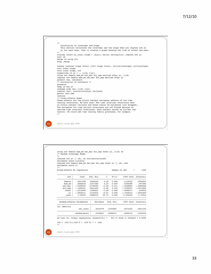
/* ! Correlation of intercept and Slope! This section calculates the intercept and the slope when you regress sch on ! yr for each case, then it creates a graph showing the link of school and year. !*/!statsby inter=_b[_cons] slope = _b[yr], by(id) saving(ols): regress sch yr!sort id!merge id using ols!drop _merge!
twoway (scatter slope inter) (lfit slope inter), xtitle(Intercept) ytitle(Slope)!corr inter slope!corr inter slope, cov!xtdescribe if yr < ., i(id) t(yr)!xtsum sch female mom_ed nev_mar div_sep married other yr, i(id)!regress sch female mom_ed nev_mar div_sep married other yr!predict res, residuals!/* Correlation of residuals */!preserve!keep id res yr!reshape wide res, i(id) j(yr)!tabstat res*, statistics(count variance) !pwcorr res*,obs!restore!/* Fixed effects model !These effects are the within subject estimates effects of the time !varying covariates. We have none. The time invariant covariates have !no within subject variance and hence cannot be estimated (are dropped).!The estimates for time variant covariance are not biased because of !omitted time invariant covariates. Each subject serves as his/her own!control. We could add time varying family processes, for example.!*/!
Alan C. Acock, July, 2010 65
xtreg sch female mom_ed nev_mar div_sep other yr, i(id) fe!/* Random Intercept Model !*/!xtmixed sch yr || id:, ml cov(unstructured)!estimates store riyronly!xtmixed sch female mom_ed nev_mar div_sep other yr || id:, mle!estimates store ri!/*!Mixed-effects ML regression Number of obs = 1386!
------------------------------------------------------------------------------! sch | Coef. Std. Err. z P>|z| [95% Conf. Interval]!-------------+----------------------------------------------------------------! female | .2047184 .0465646 4.40 0.000 .1134535 .2959834! mom_ed | .0666624 .0157266 4.24 0.000 .0358388 .097486! nev_mar | -.2009229 .0785592 -2.56 0.011 -.3548962 -.0469496! div_sep | -.1490321 .0621459 -2.40 0.016 -.2708357 -.0272284! other | -.2215656 .1206561 -1.84 0.066 -.4580471 .014916! yr | -.0828231 .0120616 -6.87 0.000 -.1064634 -.0591829! _cons | 3.52834 .0888233 39.72 0.000 3.354249 3.70243!------------------------------------------------------------------------------!------------------------------------------------------------------------------! Random-effects Parameters | Estimate Std. Err. [95% Conf. Interval]!-----------------------------+------------------------------------------------!id: Identity |! sd(_cons) | .4432578 .0190082 .4075252 .4821236!-----------------------------+------------------------------------------------! sd(Residual) | .4194833 .0098414 .4006312 .4392225!------------------------------------------------------------------------------!LR test vs. linear regression: chibar2(01) = 353.71 Prob >= chibar2 = 0.0000!
ICC = .443^2/(.443^2 + .419^2) = = .528!*/!
7/12/10
34
Alan C. Acock, July, 2010 66
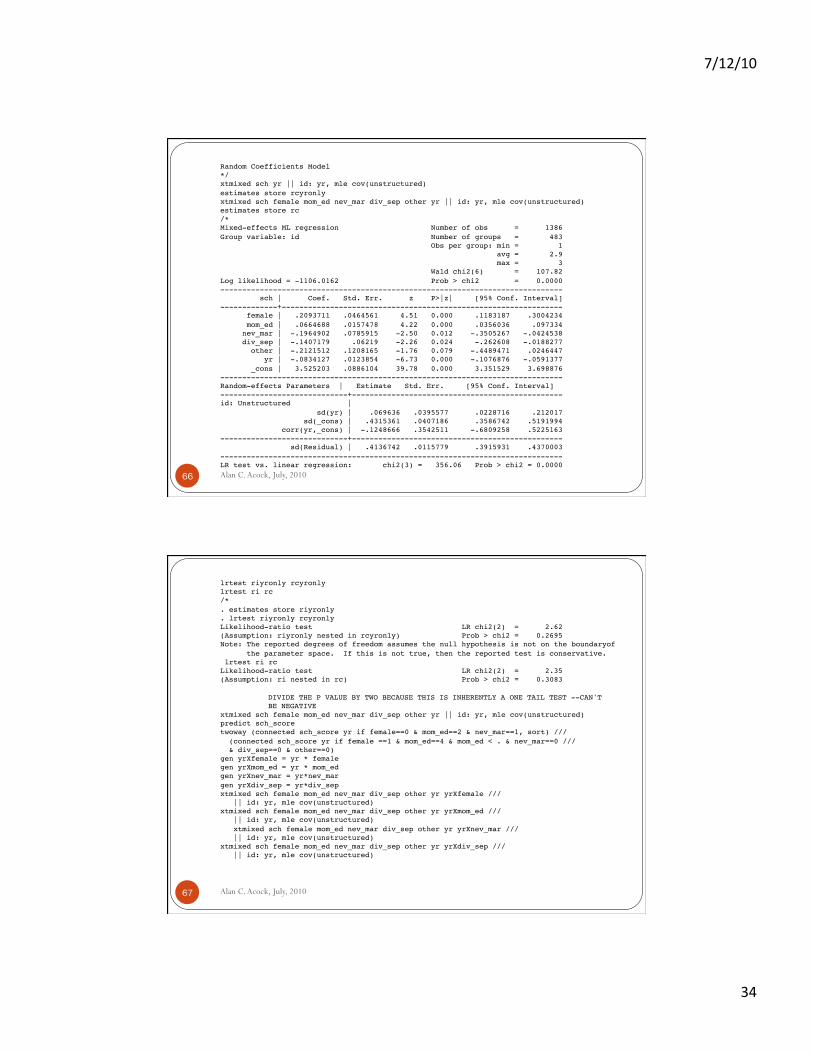
Random Coefficients Model!*/!xtmixed sch yr || id: yr, mle cov(unstructured)!estimates store rcyronly!xtmixed sch female mom_ed nev_mar div_sep other yr || id: yr, mle cov(unstructured)!estimates store rc!/*!Mixed-effects ML regression Number of obs = 1386!Group variable: id Number of groups = 483! Obs per group: min = 1! avg = 2.9! max = 3! Wald chi2(6) = 107.82!Log likelihood = -1106.0162 Prob > chi2 = 0.0000!------------------------------------------------------------------------------! sch | Coef. Std. Err. z P>|z| [95% Conf. Interval]!-------------+----------------------------------------------------------------! female | .2093711 .0464561 4.51 0.000 .1183187 .3004234! mom_ed | .0664688 .0157478 4.22 0.000 .0356036 .097334! nev_mar | -.1964902 .0785915 -2.50 0.012 -.3505267 -.0424538! div_sep | -.1407179 .06219 -2.26 0.024 -.262608 -.0188277! other | -.2121512 .1208165 -1.76 0.079 -.4489471 .0246447! yr | -.0834127 .0123854 -6.73 0.000 -.1076876 -.0591377! _cons | 3.525203 .0886104 39.78 0.000 3.351529 3.698876!------------------------------------------------------------------------------!Random-effects Parameters | Estimate Std. Err. [95% Conf. Interval]!-----------------------------+------------------------------------------------!id: Unstructured |! sd(yr) | .069636 .0395577 .0228716 .212017! sd(_cons) | .4315361 .0407186 .3586742 .5191994! corr(yr,_cons) | -.1248666 .3542511 -.6809258 .5225163!-----------------------------+------------------------------------------------! sd(Residual) | .4136742 .0115779 .3915931 .4370003!------------------------------------------------------------------------------!LR test vs. linear regression: chi2(3) = 356.06 Prob > chi2 = 0.0000!
Alan C. Acock, July, 2010 67
lrtest riyronly rcyronly!lrtest ri rc!/*!. estimates store riyronly!. lrtest riyronly rcyronly!Likelihood-ratio test LR chi2(2) = 2.62!(Assumption: riyronly nested in rcyronly) Prob > chi2 = 0.2695!Note: The reported degrees of freedom assumes the null hypothesis is not on the boundaryof! the parameter space. If this is not true, then the reported test is conservative.! lrtest ri rc!Likelihood-ratio test LR chi2(2) = 2.35!(Assumption: ri nested in rc) Prob > chi2 = 0.3083!
!DIVIDE THE P VALUE BY TWO BECAUSE THIS IS INHERENTLY A ONE TAIL TEST --CAN'T! !BE NEGATIVE!xtmixed sch female mom_ed nev_mar div_sep other yr || id: yr, mle cov(unstructured)!predict sch_score!twoway (connected sch_score yr if female==0 & mom_ed==2 & nev_mar==1, sort) ///! (connected sch_score yr if female ==1 & mom_ed==4 & mom_ed < . & nev_mar==0 ///! & div_sep==0 & other==0) !gen yrXfemale = yr * female!gen yrXmom_ed = yr * mom_ed!gen yrXnev_mar = yr*nev_mar!gen yrXdiv_sep = yr*div_sep!xtmixed sch female mom_ed nev_mar div_sep other yr yrXfemale ///! || id: yr, mle cov(unstructured)!xtmixed sch female mom_ed nev_mar div_sep other yr yrXmom_ed ///! || id: yr, mle cov(unstructured)! xtmixed sch female mom_ed nev_mar div_sep other yr yrXnev_mar ///! || id: yr, mle cov(unstructured) !xtmixed sch female mom_ed nev_mar div_sep other yr yrXdiv_sep ///! || id: yr, mle cov(unstructured)!