Multilevel Monte Carlo Path Simulation - University of … option to sell US dollars at a specific...
34
Multilevel Monte Carlo Path Simulation Mike Giles [email protected] Oxford University Computing Laboratory 15th Scottish Computational Mathematics Symposium Multilevel Monte Carlo – p. 1/34
Transcript of Multilevel Monte Carlo Path Simulation - University of … option to sell US dollars at a specific...

Multilevel Monte CarloPath Simulation
Mike Giles
Oxford University Computing Laboratory
15th Scottish Computational Mathematics Symposium
Multilevel Monte Carlo – p. 1/34

SDEs in Finance
In computational finance, stochastic differential equationsare used to model the behaviour of
stocks
interest rates
exchange rates
weather
electricity/gas demand
crude oil prices
. . .
The stochastic term accounts for the uncertainty ofunpredictable day-to-day events.
Multilevel Monte Carlo – p. 2/34

SDEs in Finance
These models are then used to calculate “fair” prices for ahuge range of financial options:
an option to sell a stock portfolio at a specific price in 2years time
an option to buy aviation fuel at a specific price in 6months time
an option to sell US dollars at a specific exchange ratein 3 years time
In most cases, the buyer of the financial option is trying toreduce their risk.
Multilevel Monte Carlo – p. 3/34

SDEs in Finance
Examples:
Geometric Brownian motion (Black-Scholes model forstock prices)
dS = r S dt + σ S dW
Cox-Ingersoll-Ross model (interest rates)
dr = α(b − r) dt + σ√
r dW
Heston stochastic volatility model (stock prices)
dS = r S dt +√
V S dW1
dV = λ (σ2−V ) dt + ξ√
V dW2
with correlation ρ between dW1 and dW2
Multilevel Monte Carlo – p. 4/34
Generic Problem
Stochastic differential equation with general drift andvolatility terms: SDE with general drift and volatility terms:
dS(t) = a(S, t) dt + b(S, t) dW (t)
W (t) is a Wiener variable with the properties that for anyq<r<s<t, W (t)−W (s) is Normally distributed with mean 0and variance t−s, independent of W (r)−W (q).
In many finance applications, we want to compute theexpected value of an option dependent on the terminal state
P = f(S(T ))
with a uniform Lipschitz bound,
|f(U) − f(V )| ≤ c ‖U − V ‖ , ∀ U, V.Multilevel Monte Carlo – p. 5/34
Standard MC Approach
Euler discretisation with timestep h:
Sn+1 = Sn + a(Sn, tn)h + b(Sn, tn) ∆Wn
Simplest estimator for expected payoff is an average of N
independent path simulations:
Y = N−1N∑
i=1
f(S(i)T/h
)
Multilevel Monte Carlo – p. 6/34

Standard MC Approach
Two kinds of errors:
statistical error, due to finite number of paths
V [Y ] = N−1V [f(ST/h)]
so r.m.s. error = O(N−1/2).
discretisation bias, due to finite number of timestepsweak convergence – O(h) error in expected payoff
strong convergence – O(h1/2) error in individual path
Multilevel Monte Carlo – p. 7/34

Standard MC Approach
Mean Square Error is O(N−1 + h2
)
first term comes from variance of estimator
second term comes from bias due to weak convergence
To make this O(ε2) requires
N = O(ε−2), h = O(ε) =⇒ cost = O(N h−1) = O(ε−3)
Aim is to improve this cost to O(ε−2(log ε)2
)
Multilevel Monte Carlo – p. 8/34

Multigrid
A powerful technique for solving PDE discretisations:
Fine gridmore accurate
more expensive
Coarse gridless accurate
less expensive
Multilevel Monte Carlo – p. 9/34

Multigrid
Multigrid combines calculations on a nested sequence ofgrids to get the accuracy of the finest grid at a much lowercomputational cost.
We will use a similar idea to achieve variance reduction inMonte Carlo path calculations, combining simulations withdifferent numbers of timesteps – same accuracy as finestcalculations, but at a much lower computational cost.
Multilevel Monte Carlo – p. 10/34

Other Research
In Dec. 2005, Ahmed Kebaier published an article inAnnals of Applied Probability describing a two-level methodwhich reduces the cost to O
(ε−2.5
).
Also in Dec. 2005, Adam Speight wrote a workingpaper describing a similar multilevel use of controlvariates, but without an analysis of its complexity.
There are also close similarities to a multileveltechnique developed by Stefan Heinrich for parametricintegration (Journal of Complexity, 1998)
Multilevel Monte Carlo – p. 11/34

Multilevel MC Approach
Consider multiple sets of simulations with differenttimesteps hl = 2−l T, l = 0, 1, . . . , L, and payoff Pl
E[PL] = E[P0] +L∑
l=1
E[Pl−Pl−1]
Expected value is same – aim is to reduce variance ofestimator for a fixed computational cost.
Key point: approximate E[Pl−Pl−1] using Nl simulationswith Pl and Pl−1 obtained using same Brownian path.
Yl = N−1l
Nl∑
i=1
(P
(i)l −P
(i)l−1
)
Multilevel Monte Carlo – p. 12/34

Multilevel MC Approach
Discrete Brownian path at different levels
0 0.1 0.2 0.3 0.4 0.5 0.6 0.7 0.8 0.9 1−1
−0.5
0
0.5
1
1.5
2
2.5
3
3.5
P7
P6
P5
P4
P3
P2
P1
P0
Multilevel Monte Carlo – p. 13/34

Multilevel MC Approach
each level adds more detail to Brownian path
E[Pl−Pl−1] reflects impact of that extra detail on thepayoff
different timescales handled by different levels– similar to different wavelengths being handled bydifferent grids in multigrid
Multilevel Monte Carlo – p. 14/34

Multilevel MC Approach
Using independent paths for each level, the variance of thecombined estimator is
V
[L∑
l=0
Yl
]=
L∑
l=0
N−1l Vl, Vl ≡ V [Pl−Pl−1],
and the computational cost is proportional toL∑
l=0
Nl h−1l .
Hence, the variance is minimised for a fixed computationalcost by choosing Nl to be proportional to
√Vl hl.
The constant of proportionality can be chosen so that thecombined variance is O(ε2).
Multilevel Monte Carlo – p. 15/34

Multilevel MC Approach
For the Euler discretisation and the Lipschitz payoff function
V [Pl−P ] = O(hl) =⇒ V [Pl−Pl−1] = O(hl)
and the optimal Nl is asymptotically proportional to hl.
To make the combined variance O(ε2) requires
Nl = O(ε−2Lhl).
To make the bias O(ε) requires
L = log2 ε−1 + O(1) =⇒ hL = O(ε).
Hence, we obtain an O(ε2) MSE for a computational costwhich is O(ε−2L2) = O(ε−2(log ε)2).
Multilevel Monte Carlo – p. 16/34

Multilevel MC Approach
Theorem: Let P be a functional of the solution of a stochastic o.d.e.,
and Pl the discrete approximation using a timestep hl = M−l T .
If there exist independent estimators Yl based on Nl Monte Carlo
samples, and positive constants α≥ 12 , β, c1, c2, c3 such that
i) E[Pl − P ] ≤ c1 hαl
ii) E[Yl] =
E[P0], l = 0
E[Pl − Pl−1], l > 0
iii) V [Yl] ≤ c2 N−1l h
βl
iv) Cl, the computational complexity of Yl, is bounded by
Cl ≤ c3 Nl h−1l
Multilevel Monte Carlo – p. 17/34
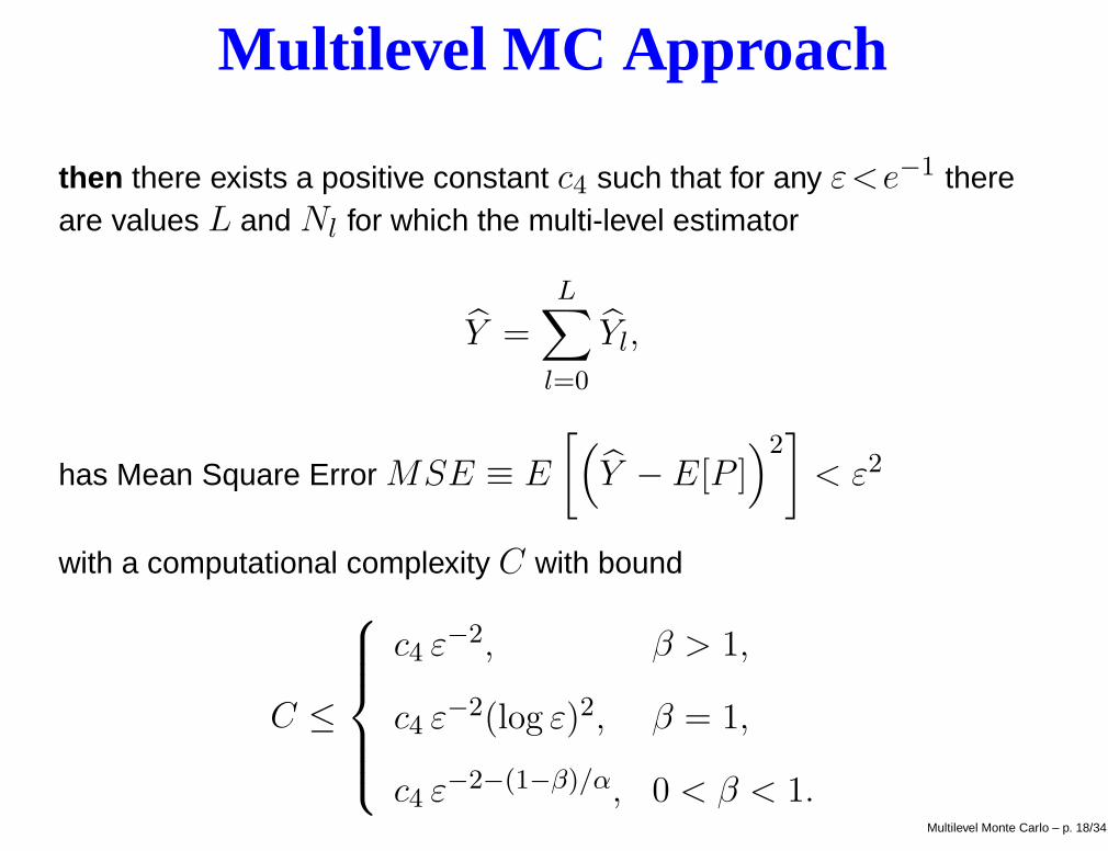
Multilevel MC Approach
then there exists a positive constant c4 such that for any ε<e−1 thereare values L and Nl for which the multi-level estimator
Y =L∑
l=0
Yl,
has Mean Square Error MSE ≡ E
[(Y − E[P ]
)2]
< ε2
with a computational complexity C with bound
C ≤
c4 ε−2, β > 1,
c4 ε−2(log ε)2, β = 1,
c4 ε−2−(1−β)/α, 0 < β < 1.Multilevel Monte Carlo – p. 18/34

Results
Geometric Brownian motion:
dS = r S dt + σ S dW, 0 < t < 1,
S(0)=1, r=0.05, σ=0.2
Heston model:
dS = r S dt +√
V S dW1, 0 < t < 1
dV = λ (σ2−V ) dt + ξ√
V dW2,
S(0)=1, V (0)=0.04, r=0.05, σ=0.2, λ=5, ξ=0.25, ρ=−0.5
All calculations use M =4, more efficient than M =2.
Multilevel Monte Carlo – p. 19/34
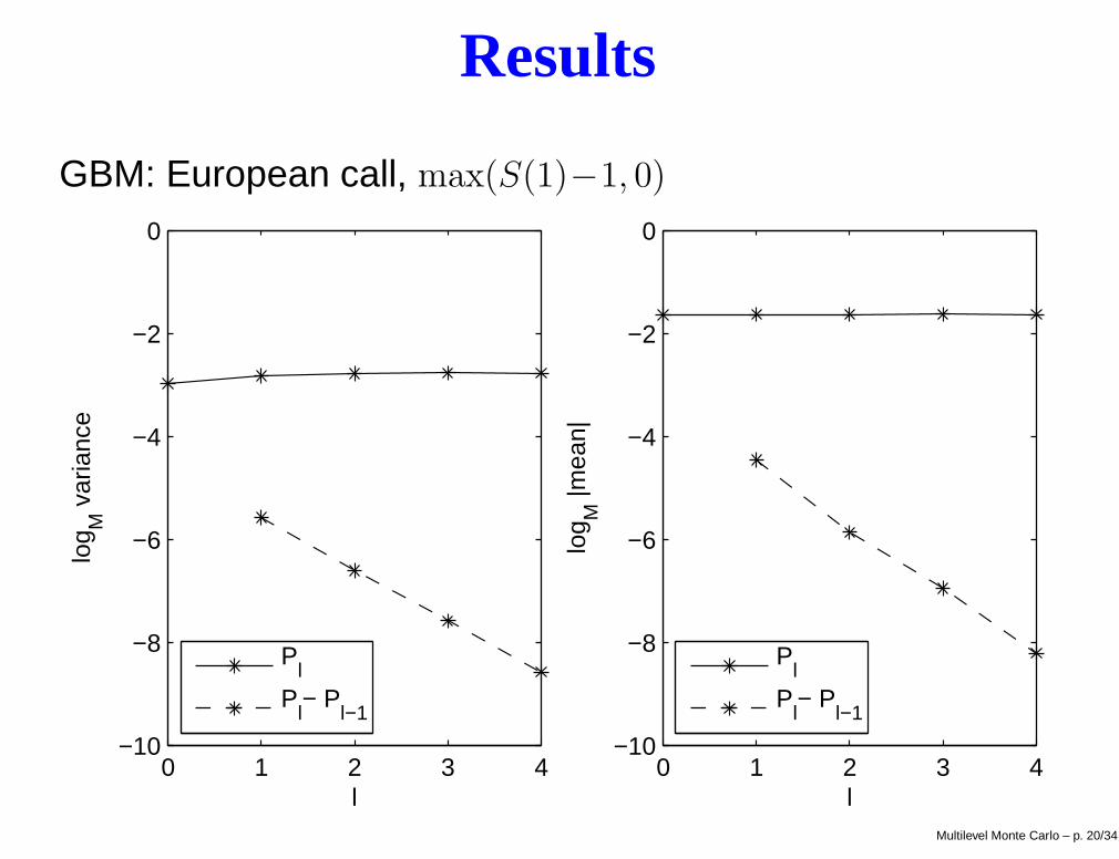
Results
GBM: European call, max(S(1)−1, 0)
0 1 2 3 4−10
−8
−6
−4
−2
0
l
log M
var
ianc
e
Pl
Pl− P
l−1
0 1 2 3 4−10
−8
−6
−4
−2
0
l
log M
|mea
n|
Pl
Pl− P
l−1
Multilevel Monte Carlo – p. 20/34

Results
GBM: European call, max(S(1)−1, 0)
0 1 2 3 410
2
104
106
108
1010
l
Nl
ε=0.00005ε=0.0001ε=0.0002ε=0.0005ε=0.001
10−4
10−3
10−2
10−1
100
101
ε
ε2 Cos
t
Std MCMLMC
Multilevel Monte Carlo – p. 21/34
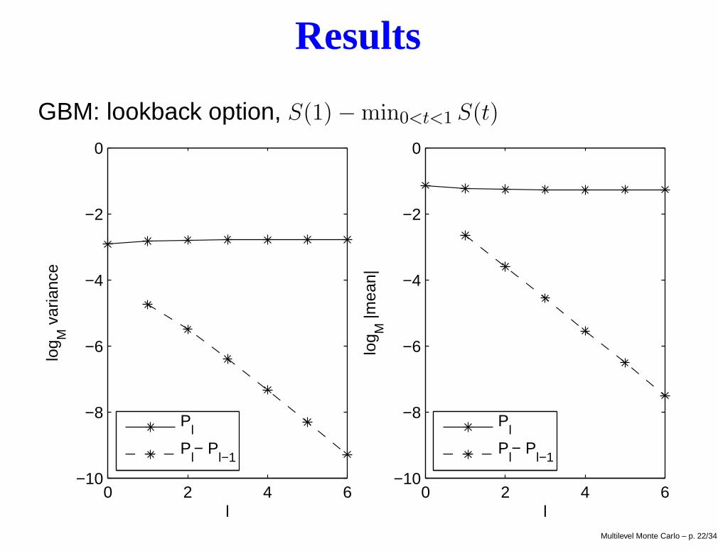
Results
GBM: lookback option, S(1) − min0<t<1 S(t)
0 2 4 6−10
−8
−6
−4
−2
0
l
log M
var
ianc
e
Pl
Pl− P
l−1
0 2 4 6−10
−8
−6
−4
−2
0
l
log M
|mea
n|
Pl
Pl− P
l−1
Multilevel Monte Carlo – p. 22/34

Results
GBM: lookback option, S(1) − min0<t<1 S(t)
0 2 4 610
2
104
106
108
1010
l
Nl
ε=0.00005ε=0.0001ε=0.0002ε=0.0005ε=0.001
10−4
10−3
10−1
100
101
102
ε
ε2 Cos
t
Std MCMLMC
Multilevel Monte Carlo – p. 23/34

Results
Heston model: European call
0 1 2 3 4−10
−8
−6
−4
−2
0
l
log M
var
ianc
e
Pl
Pl− P
l−1
0 1 2 3 4−10
−8
−6
−4
−2
0
l
log M
|mea
n|
Pl
Pl− P
l−1
Multilevel Monte Carlo – p. 24/34
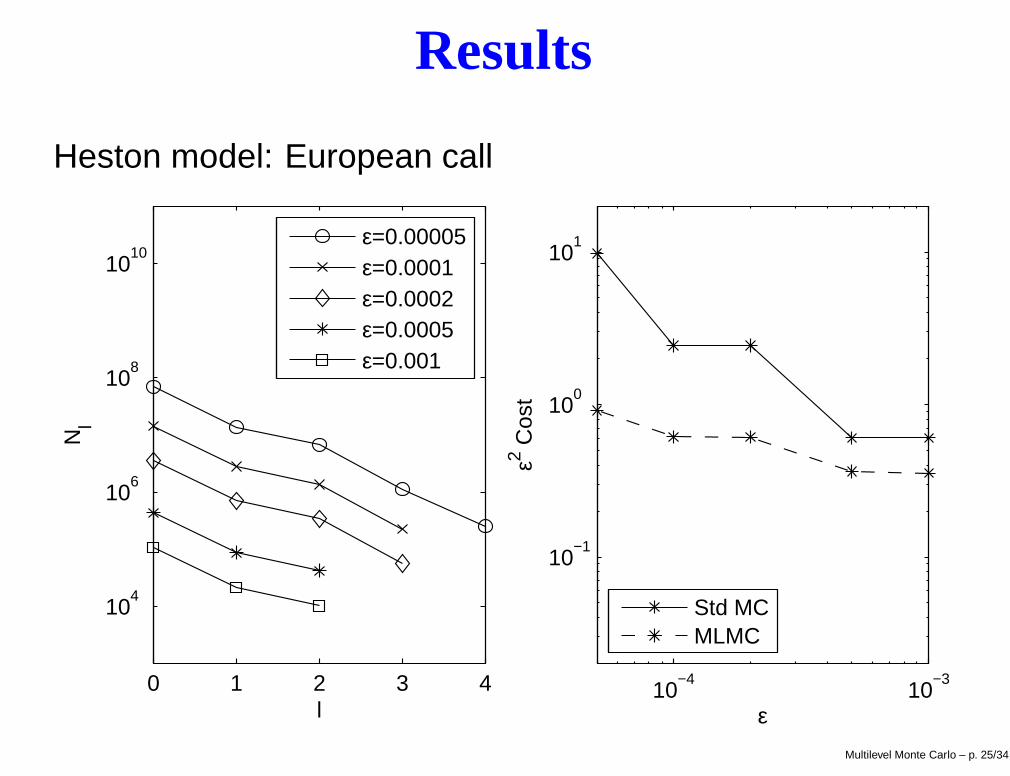
Results
Heston model: European call
0 1 2 3 4
104
106
108
1010
l
Nl
ε=0.00005ε=0.0001ε=0.0002ε=0.0005ε=0.001
10−4
10−3
10−1
100
101
ε
ε2 Cos
t
Std MCMLMC
Multilevel Monte Carlo – p. 25/34

Conclusions
Results so far:
improved order of complexity
easy to implement
significant benefits for model problems
Current research:
use of Milstein method (and antithetic variables inmulti-dimensional case) to reduce complexity to O(ε−2)
adaptive sampling to treat discontinuous payoffs andpathwise derivatives for Greeks
use of quasi-Monte Carlo methods, to reducecomplexity towards O(ε−1)
Multilevel Monte Carlo – p. 26/34

Working Paper
M.B. Giles, “Multi-level Monte Carlo path simulation”Oxford University Computing Laboratory
Numerical Analysis Report NA-06/03
www.comlab.ox.ac.uk/mike.giles/finance.html
Email: [email protected]
Acknowledgements:
Paul Glasserman and Mark Broadie for early feedback
Microsoft for current research funding
Multilevel Monte Carlo – p. 27/34
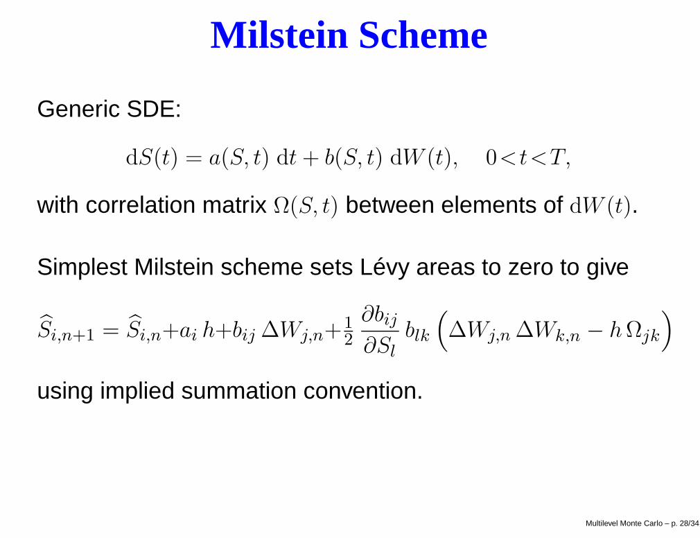
Milstein Scheme
Generic SDE:
dS(t) = a(S, t) dt + b(S, t) dW (t), 0<t<T,
with correlation matrix Ω(S, t) between elements of dW (t).
Simplest Milstein scheme sets Lévy areas to zero to give
Si,n+1 = Si,n+ai h+bij ∆Wj,n+12
∂bij
∂Slblk
(∆Wj,n ∆Wk,n − hΩjk
)
using implied summation convention.
Multilevel Monte Carlo – p. 28/34

Milstein Scheme
In scalar case:
O(h) strong convergence
O(ε−2) complexity for Lipschitz payoffs
O(ε−2) complexity for lookback, barrier and digitaloptions using carefully constructed estimators
In multi-dimensional case:
still only O(h1/2) strong convergence
but Sn − E[S |Wn] = O(h)
Multilevel Monte Carlo – p. 29/34

Milstein Scheme
If a coarse path with timestep 2h is constructed using
∆W cn =
√2h Yn
where the Yn are N(0, 1) random variables, and the finepath uses a Brownian Bridge construction with
∆W fn = 1
2
√2h (Yn+Zn), ∆W
fn+ 1
2
= 12
√2h (Yn−Zn).
where the Zn are also N(0, 1) random variables, thenperturbation analysis shows that the O(h1/2) differencebetween the two paths comes from a sum of termsproportional to
Yj,nZk,n − Yk,nZj,n.
Multilevel Monte Carlo – p. 30/34

Milstein Scheme
Using the idea of antithetic variables, we use the estimator
Yl = N−1l
Nl∑
i=1
(12
(P
(i)l +P
(i)∗l
)− P
(i)l−1
),
where P(i)∗l is based on the same coarse path Yn, but with
Zn replaced by −Zn, which leads to the cancellation of theleading order error proportional to Zn.
V [Yl] = O(h2) for smooth payoffs, O(h3/2) for Lipschitz
in both cases, gives O(ε−2) complexity for O(ε) accuracy
Multilevel Monte Carlo – p. 31/34
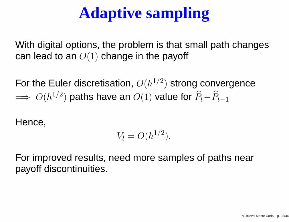
Adaptive sampling
With digital options, the problem is that small path changescan lead to an O(1) change in the payoff
For the Euler discretisation, O(h1/2) strong convergence=⇒ O(h1/2) paths have an O(1) value for Pl−Pl−1
Hence,Vl = O(h1/2).
For improved results, need more samples of paths nearpayoff discontinuities.
Multilevel Monte Carlo – p. 32/34

Adaptive sampling
Two ideas for adaptive sampling are both based onBrownian Bridge constructions, using coarse timesteprealisations to decide which paths are important
idea 1: start with relatively few paths, and sub-dividethose which look interesting (splitting)
idea 2: start with lots of paths, and prune those whichare unimportant (Russian roulette)
use path weights to ensure estimator remains unbiased
initial results (combining 2 ideas to keep a fixed numberof paths) look good for a digital option, and it shouldalso handle barrier options
Multilevel Monte Carlo – p. 33/34

Quasi-Monte Carlo
Quasi-Monte Carlo methods can offer greatly improvedconvergence with respect to the number of samples N :
in the best case, O(N−1+δ) error for arbitrary δ > 0,instead of O(N−1/2)
depends on knowledge/identification of “importantdimensions” in an application
Brownian BridgePrincipal Component Analysis
confidence intervals can be obtained by usingrandomized QMC
working with Sloan, Kuo and Waterhouse, will try bothrank-1 lattice rules and Sobol sequences
Multilevel Monte Carlo – p. 34/34