Multicut Benders Decomposition Algorithm for Process Supply Chain Planning under Uncertainty

Fengqi You1 and Ignacio E. Grossmann2 1Mathematics and Computer Science Division, Argonne National Laboratory, Argonne,

IL 60439 2Dept. of Chemical Engineering, Carnegie Mellon University, Pittsburgh, PA 15213

February 7, 2011

Abstract In this paper, we present a multicut version of the Benders decomposition method for

solving two-stage stochastic linear programming problems, including stochastic mixed-

integer programs with only continuous recourse (two-stage) variables. The main idea is to

add one cut per realization of uncertainty to the master problem in each iteration, that is,

as many Benders cuts as the number of scenarios added to the master problem in each

iteration. Two examples are presented to illustrate the application of the proposed

algorithm. One involves production-transportation planning under demand uncertainty,

and the other one involves multiperiod planning of global, multiproduct chemical supply

chains under demand and freight rate uncertainty. Computational studies show that while

both the standard and the multicut versions of the Benders decomposition method can

solve large-scale stochastic programming problems with reasonable computational effort,

significant savings in CPU time can be achieved by using the proposed multicut

algorithm.

Keywords: Benders decomposition, stochastic programming, planning, supply chain

1. Introduction Many problems for supply chain planning under uncertainty can be formulated as

two-stage stochastic programming problems with fixed recourse (Birge & Louveaux,

1997; Infanger, 1994; Shapiro, 2008). In the two-stage framework, the first-stage

decisions are made “here-and-now” prior to the resolution of uncertainty, while the

second-stage decisions are postponed in a “wait-and-see” mode after the uncertainties

are revealed. The scenario planning approach is used to represent the uncertainties

through a number of discrete realizations of the stochastic quantities, constituting

distinct scenarios. The objective is to find a solution that performs well on average

under all scenarios. This approach provides a straightforward way to account for

uncertainty, but the resulting stochastic programming models are often

computationally demanding because their model size increases exponentially as the

number of scenarios increases.

In order to address the computational challenge, a number of methods have been

proposed for the solution of two-stage stochastic programming problems

(Ruszczyński, 1997), such as Benders decomposition (Benders, 1962; Van Slyke &

Wets, 1969), stochastic decomposition (Higle & Sen, 1991), subgradient

decomposition (Sen, 1993; Sen and Huang, 2009), disjunctive decomposition (Ntaimo,

2010), and nested decomposition (Archibald et al., 1999). Among these methods,

Benders decomposition (Benders, 1962), also called the L-shaped method, has

become the major approach to tackle stochastic programming problems because of its

ease of implementation. This method takes advantage of the special decomposable

structure of the two-stage stochastic programming model and generates duality cuts

based on the subgradient information iteratively. Since the standard Benders

decomposition returns only one cut to the master problem in each iteration, its

convergence might be slow for some computationally demanding problems (Birge &

Louveaux, 1997). To address this issue, numerous researchers have proposed variants

to accelerate the algorithm (Bahn et al., 1995; Escudero et al., 2007; Fragniere et al.,

2000; Gerd Infanger, 1993; Latorre et al., 2009; Linderoth & Wright, 2003; Mulvey &

Ruszczynski, 1995; Ruszczynski, 1993; Saharidis & Ierapetritou, 2010; Saharidis et

al., 2010; Trukhanov et al., 2010).

In this paper, we consider the solution methods for stochastic linear programming

problems and stochastic mixed-integer linear programs with only continuous recourse.

-2-

We first describe a multicut version of the Benders decomposition, which is a variant

of the standard Benders decomposition method but converges faster in general cases.

We discuss the theory behind this algorithm and prove its convergence. Two

applications of this algorithm are then presented to illustrate the effectiveness of this

method. The first application involves production-transportation planning under

demand uncertainty. Because of the relatively small problem size, the global optimal

solution of this problem can easily be obtained to validate the proposed solution

approach and illustrate its effectiveness. The second application involves global

chemical supply chain planning under uncertainty, which originates from a real-world

application in the Dow Chemical Company. The model was taken from the authors’

earlier work (You et al., 2009). Three testing data sets with different sizes are

considered. In both applications, the results show that the multicut version of the

Benders decomposition method requires fewer iterations and less computational time

than does the standard version to obtain a solution with a specified optimality

tolerance.

The rest of this paper is organized as follows. Section 2 presents the multicut

Benders decomposition algorithm, for problems where the first-stage decision

variables can include both discrete and continuous variables, while the second-stage

decision variables must all be continuous variables. The problem statements, model

formulations, and computational results for the two applications are given in Sections

3 and 4. In Section 5, we summarize our conclusions.

2. Multicut Benders Decomposition Algorithm Consider the following general form of the two-stage stochastic programming

model (P0):

(P0) T

,min

s

Ts s sx y s S

c x p q y∈

+∑ (1)

s.t. , 0Ax b x= ≥ (2)

, ) 0, s s s sWy h T x y(w s S= − ≥ ∈ (3)

where x is a vector that stands for the first-stage decision variables, which may

include 0-1 variables; sy are the continuous second-stage decisions for each

scenario s ; and b are parameter matrices independent of the scenarios; and , A W sh

-3-

and sT are parameter matrices for each scenario s S∈ .

The expanded version of the general model (P0) is given in equation (4). The

problem has a special “angular” form, which can be decomposed into a master

problem and a number of scenario subproblems.

Master problem

Scenario subproblems

Master problemMaster problem

Scenario subproblems

(4)

The special decomposable structure of (4) is suitable for Benders decomposition

because it takes advantage of subgradient information to construct convex estimates

of the recourse function and iteratively generates a Benders cut to be added to the

decomposed master problem (Benders, 1962; Van Slyke & Wets, 1969). In the first

step, a decomposed subproblem with those constraints that do not include the second-

stage variables is solved to obtain the values of the first-stage decisions. Then we fix

the first-stage decisions and solve all the scenario subproblems that include second-

stage decisions, in order to obtain the optimal values of the second-stage decisions.

Let , the value function, be the objective function value of each scenario

subproblem .

( )sQ x

sTmin

s

( )s s syQ x q y =

s.t. , ) 0s s s sWy h T x y(w= − ≥

≥

(5)

The reformulation of (P0) is then as follows.

(P0) (6) Tmin ( )s sx s Sc x p Q x

∈

+∑

s.t. , 0Ax b x= (7)

To solve (P0), we can take advantage of the dual properties of (6) by introducing

a new variable θ for ( )s ss S

p Q x∈∑ and iterating between the master problem (P1) and

the scenario subproblems (P2).

The master problem (P1) is given by

-4-

(P1) T

,min

xc x

θθ+

s.t. , 1iter iterd x e iter ..Nθ ≥ + = (8)

, 0Ax b x= ≥

while the subproblem (P2) for scenario is given by s

(P2) T min s

s syq y

s.t. , ) 0s s s sWy h T x y(w= − ≥ (9)

where the inequalities in (P1) are the “cuts” that link the master problem and the

scenario subproblems. Here, and are coefficients for the Benders cut; they are

given by

ld le

,iter T

s iter s ss S

d p π∈

=∑ T (10)

,iter T

s iter s ss S

e p π∈

=∑ h (11)

where sπ are the optimal dual vectors of constraint (5) in the subproblem (P2) for

scenario s .

In this paper, we assume that the problem (P0) has complete recourse and that

(P2) is always feasible. Under this assumption, feasibility cuts are not present in the

master problem (P1). Our algorithms and this analysis can be generalized to handle

situations in which the aforementioned assumption does not hold; but for the sake of

simplifying the analysis, we avoid discussing this more general case here.

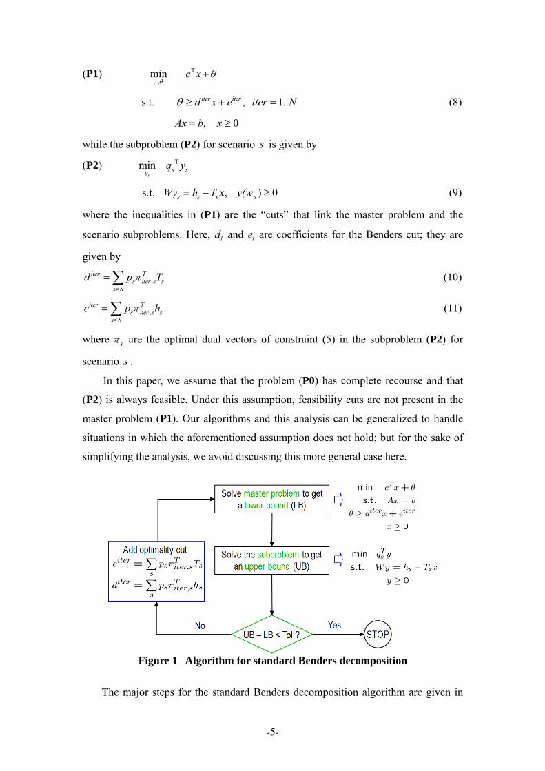
Figure 1 Algorithm for standard Benders decomposition

The major steps for the standard Benders decomposition algorithm are given in

-5-

Figure 1. In this algorithm, we first solve the master problem to obtain a lower bound

of the objective value. We then fix all the first-stage decisions and solve each scenario

subproblem to get an upper bound. If the lower bound and the upper bound are within

a tolerance, then the algorithm stops. Otherwise, we use the duals of the scenario

subproblems to add a Benders cut and return to the master problem.

The standard Benders decomposition algorithm only returns one cut per iteration

to the master problem. For large-scale problem, its convergence might be slow and the

algorithm might need many iterations to reach a predefined optimality tolerance.

To speed up the algorithm, we can decompose the variable θ by scenarios to

return as many cuts as the number of scenarios in each iteration. In this variant, the

master problem is then given by (P3).

(P3) T

,min

ss sx s S

c x pθ

θ∈

+∑

s.t. , 1 , 1iter iters s sd x e iter ..N s ..Sθ ≥ + = = (12)

, 0Ax b x= >

The coefficients sld and sle for the cut (12) are updated as follows

,iter Ts iter s sd π= T (13)

,iter Ts iter s se π= h (14)

where sπ are the optimal dual vectors of constraint (5) in the subproblem (P2) for

scenario s .

Figure 2 Algorithm for multicut Benders method

The algorithm framework for the multicut Benders algorithm is similar to that for

-6-

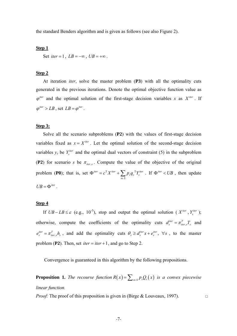
the standard Benders algorithm and is given as follows (see also Figure 2).

Step 1

Set , , UB . 1iter = LB = −∞ = +∞

Step 2

At iteration iter, solve the master problem (P3) with all the optimality cuts

generated in the previous iterations. Denote the optimal objective function value as iterϕ and the optimal solution of the first-stage decision variables x as iterX . If

, set iterϕ LB> iterLB ϕ= .

Step 3:

Solve all the scenario subproblems (P2) with the values of first-stage decision

variables fixed as iterx X=r

,iter

. Let the optimal solution of the second-stage decision

variables ys be and the optimal dual vectors of constraint itesY (5) in the subproblem

(P2) for scenario s be sπ . Compute the value of the objective of the original

problem (P0); that is, set T Titer iter iters s s

s Sc X p q Y

∈

Φ = +∑ . If , then update

.

iter UBΦ <

iterUB = Φ

Step 4

If UB LB ε− ≤ (e.g., 10-3), stop and output the optimal solution ( iterX , );

otherwise, compute the coefficients of the optimality cuts

itersY

,Titer

s iter sπ sd T and =

,Titer

s iter s shπe = , and add the optimality cuts , to the master

problem (P2). Then, set , and go to Step 2.

, iter iters s sd x eθ ≥ + s∀

1iter iter= +

Convergence is guaranteed in this algorithm by the following propositions.

Proposition 1. The recourse function ( ) ( )s ss SR x p Q

∈= x∑ is a convex piecewise

linear function.

Proof: The proof of this proposition is given in (Birge & Louveaux, 1997).

-7-

( )R xProposition 2. Each optimality cut (12) supports the recourse function and

Proof: this proposition is given by (Birge & Louveaux, 1997).

Proposition 3. Given some (

( )Q x from below.

The proof of

s

iterX , iter

sθ ) such that , iter iter iter iters s sd X e sθ = + ∀ , then

iterX is an optimal solution of the original problem (P0

f:

).

Proo

ginal problem (P0) is equivalent to the following problem (P4). The ori

Tmin s sxc x p θ

s S∈+∑

s.t. , 0Ax b x= ≥

( )s sQ x θ≤

Based on osition Prop 2 and the duality property of (P2), we have

( ), iter iter iter iter iters s s se X d Q X sθ = + = ∀ . Therefore, ( iterX , iter

sθ ) is a feasible solution of

(P4). Since ( iterX , itersθ ) is the optimal solution of ( , i also an optimal solution

of (P4), which is equivalent to the original problem (P0).

P2) t is

Proposition 4. (Convergence) Since the algorithm generates a finite sequence of

( iterX , itersθ ) and since (

iterX ,

itersθ ) is the limit of this sequence, and

0iter iter iterθ− = , wh ficiently large integer, then limer M→ s sd x + sit

e ere M is a sufiter

X is an

inal problem (P0).

Proof:

optimal solution of the orig

roposition 2 and lim 0iter iter iters s siter M

d x e θ→

+ − = , we have ( )iters sQ Xθ =From P .

Thus, (iter iter

) is a feasible solution of problem (P4). Because X , sθ

function ( )s( ) ss SR x p

∈= Q x∑ is a convex piecewise linear function as shown in

Proposition 1, (iter

X , itersθ ) is also an optimal solution of (P4), which is equivalent to

the original prob (P0

lem ).

We note that while the multicut L-shaped method can provide more cuts to

-8-

supp

3. Production-Transportation Planning under Uncertainty single-

peri

ort the recourse function from below and most likely reduce the number of

iterations, it introduces more variables and constraints in the master problem, which

may potentially slow the computation. This algorithm would benefit from solving it

with parallel computing, which could significantly reduce the wall-clock times.

The first application of the proposed algorithm is about a single product,

od production-transportation planning under demand uncertainty. This problem

can be formally stated as follows.

We are given a set of plants i I∈ with production capacity capi and a set of

demand zones l L∈ . The selling price at demand zone l is pricel, the unit

transportation co m plant i to demand zone l is ctri,l, the unit production cost at

plant i is cpdi, and the unit waste disposal cost in demand zone l is cusl. Here, s S∈ is

the set of scenarios, ps is the scenario probability, and demandl,s is the dem at

demand zone l of scenario s. The major decisions include the production level (prodi),

transportation amount (shipi,l), sales amount (salel,s), and unsold product amount

(unsold,s). We note that in the two-stage stochastic linear programming framework,

the production and transportation decisions are made “here and now” prior to the

resolution of demand uncertainty, whereas the sales and waste disposal decisions are

postponed in a “wait-and-see” mode after the uncertainties are revealed. Thus, the

production and transportation decisions are independent of the scenarios, whereas the

sales decisions are made for each scenario. The objective of this problem is to

maximize the total expected profit (E[profit]) by optimizing the aforementioned

decisions.

Based

st fro

and

on the problem statement, a two-stage stochastic linear programming

mod

,

el can be formulated as follows.

max [ ] , ,

,

s lE profit p price s= ⋅ ⋅ l s i ll L s S i I l L

i i s l l si I l L s S

ale ctr ship

cpd prod p cus unsold∈ ∈ ∈ ∈

∈ ∈ ∈

− ⋅

− ⋅ − ⋅ ⋅

∑∑ i l∑∑

∑ ∑∑ (15)

s.t.

prodi icap≤ , i I∀ ∈ (16)

l,i il L

prod sh∈

=∑ ip i I∀ ∈, (17)

-9-

, ,i l l s l si I

ship sale unsold∈

= +∑ , , l L∀ ∈ , s S∈ (18)

,l s l ssale demand≤ , , l L∀ ∈ , s S∈ (19)

0iprod ≥ , ,i lship ≥ , , 0l ssale ≥ , , 0l sunsold ≥0

Table 1 Probabil distribu n of deman realizations for the production-

transportation planning problem

DeZones

ity tio d

mand Demand Realization (ton) Probability

Low Medium Medium High High Low 1 0.25 0.25 150 160 170 0.5 2 100 120 135 0.25 0.5 0.25 3 250 270 300 0.25 0.5 0.25 4 300 325 350 0.3 0.4 0.3 5 600 700 800 0.3 0.4 0.3

Ta e 2 nit port cost f production-transportation planning problem ($/ton)

PlZones 1 3 4 5

bl U trans ation or the

ants/Demand

2

P1 2.49 5.21 3.76 4.85 2.07 P2 1.46 2.54 1.83 1.86 4.76 P3 3.26 3.08 2.6 3.76 4.45

In th ase study we ider a ction-transportation network with three

plants and five demand zones. The probability distribution of the demand realization

is gi

tinuous variables and 2,436 constraints. Less than one second was

need

is c cons produ

ven in Table 1. In each demand zone there are three possible demand realizations.

We assume these probabilities are independent. By considering the joint probability

distribution, we generate a total of 35=243 scenarios for this problem. The unit

production cost is $14/ton, the sales price is $24/ton, and cost of removal of unsold

products is $4/ton. The unit transportation cost between plants and demand zones is

given in Table 2.

The deterministic equivalent of the resulting two-stage stochastic linear program

includes 2,448 con

ed to obtain the optimal solution ($10,793) with 0% gap using GAMS

23.4.3/CPLEX 12 (Rosenthal, 2010), on an IBM T400 laptop with an Intel 2.53 GHz

CPU and 2 GB RAM.

To illustrate the application of the proposed multicut algorithm and compare its

-10-

perf

fference for this case

stud

ormance with that of the standard Benders decomposition, we solved this problem

with both algorithms. The results are shown in Figures 3 and 4. As can be seen from

Figure 3, the upper bounds decrease and the lower bounds increase as the number of

iterations increase. However, whereas the standard Benders method requires 22

iterations to reach the optimality tolerance, the multicut version requires only 6

iterations. The results in Figure 3 clearly show that the multicut version converges

much faster than does the standard Benders method. The reason rests mainly with the

improved approximation of the value function in (5), since a larger number of

Benders cuts are added to the master problem at each iteration.

The computational times for both algorithms show little di

y (0.15 CPU seconds for the single cut version and 0.13 CPU seconds for the

multicut version), although the multicut version requires far fewer iterations than does

the standard Benders decomposition. The main reason is that the master problem of

the multicut Benders method includes more variables and constraints (Benders cuts)

than does the standard version and thus requires longer computational time per

iteration. Another reason is that the computational times for this case study are so

short that the scaling effect and the advantage of the multicut version cannot be fully

illustrated.

Figure 3 Comparison between the standard Benders method and the multicut

version in terms of number of iterations for the production-transportation planning problem

-11-

4. Global Chemical Supply Chain Planning under Uncertainty d

by Y

d decomposition algorithms, we

solv

4.1. roblem statement

This case study can be stated as follows. We are given a midterm planning

hori

The second case study considered in this work is based on the problem describe

ou et al. (2009), which originates from a real-world application in the Dow

Chemical Company. Global supply chains in the process industries are usually large-

scale systems that can comprise hundreds or even thousands of production facilities,

distribution centers, and customers (Wassick, 2009). This case study addresses the

midterm planning for a global multiproduct chemical supply chain under demand and

freight rate uncertainty. A two-stage stochastic mixed-integer linear programming

model is used, incorporating a multiperiod planning model that takes into account the

production and inventory levels, transportation modes, times of shipments, and

customer service levels. In the two-stage framework, the production, distribution, and

inventory decisions for the current time period, which include 0-1 variables, are made

“here and now” prior to the resolution of uncertainty, while the decisions for the

remaining time periods, which only involve continuous variables, are postponed in a

“wait-and-see” mode. The problem includes a large number of uncertain parameters

as a result of the multiperiod nature and the large size of the supply chain network. A

Monte Carlo sampling approach is used to discretize the continuous probability

distribution functions and to generate the scenarios.

To demonstrate the effectiveness of the propose

e three instances for small, medium, and large supply chain networks, using both

the standard Benders decomposition method and the multicut version. We present the

problem statement, model formulation, and computational results in the following

subsections.

P

zon (for instance, one year), which can be subdivided into a number of time

periods (for instance, one month as a time period). A set of products are manufactured

and distributed through a given global supply chain that includes a large number of

worldwide customers and a number of geographically distributed plants and

distribution centers. All the facilities (plants and distribution centers) can hold

inventory and are connected to each other by an associated transportation link. Each

-12-

customer is served by one or more facilities with specified transportation links. A

simplified version of the network is shown in Figure 4. The network has multiple

echelons whereby material may flow from the manufacturing plant through several

distribution centers on its way to the final customer. Freight rates are specific to the

transportation link involved and depend on distance and mode of transport. Generally,

the transportation links are classified into two types: from one facility to another

facility (plant or distribution center) and from a facility to a customer. Some

transportation links with certain transportation modes are managed by third-party

logistics companies; these require either that no products be shipped through these

links with the corresponding transportation mode or that a minimum quantity be

shipped in each time period.

Besides the supply chain network topology, we are given the minimum and initial

inve

s arise from the customer demands and freight rates. The values

of t

determine the monthly or weekly production and inventory

leve

ntory of each facility. The inventory holding costs and the facility throughput

costs are already known, together with future monthly demand of each product by

each customer. The transportation time of each shipping lane is known and should be

taken into account.

The uncertaintie

hese uncertain parameters follow some probability distribution (such as normal

distribution) with a given mean and variance. Usually, the probability distribution of

the uncertain parameters can be obtained by fitting the historical data for different

probability distributions or can be based on expert opinions. The mean values of these

uncertain parameters typically come from forecasting, and the variances come from

historical data. We allow the demands and freight rates to have different levels of

uncertainties changing with time. For example, in January the uncertain demand of

May has a standard deviation as much as 20% of the mean value, but in April the

standard deviation of that demand of May reduces to 5% of the mean value as a result

of more accurate forecasting and information. Different levels of uncertainties are

important for the operations of industrial supply chains and should be taken into

account in the models.

The problem is to

ls of each facility, and the monthly shipping quantities between network nodes

such that the total expected cost and the total risks of the global supply chain are

minimized, while satisfying customer demands over the specified planning horizon.

-13-

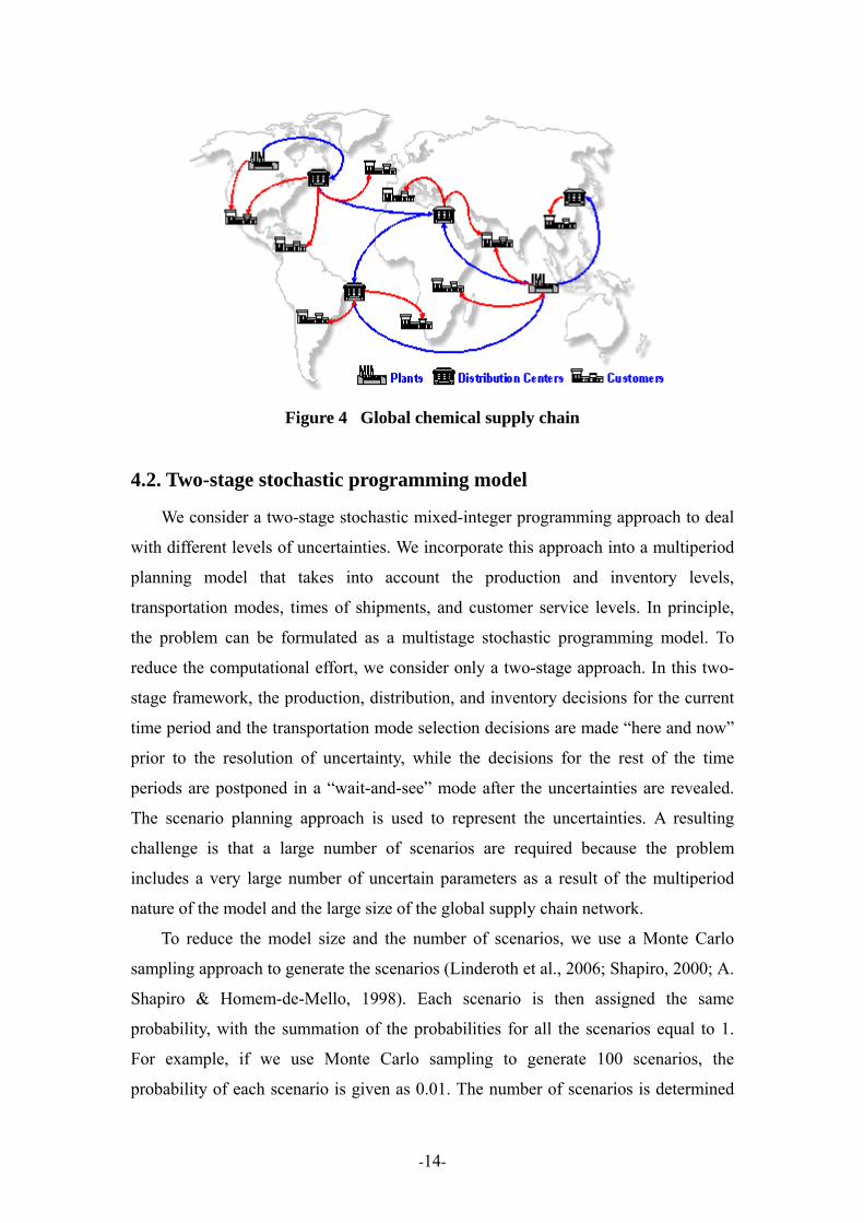
Figure 4 Global chemical supply chain

4.2. Two-stage stochastic programming model

We consider a two-stage stochastic mixed-integer programming approach to deal

with different levels of uncertainties. We incorporate this approach into a multiperiod

planning model that takes into account the production and inventory levels,

transportation modes, times of shipments, and customer service levels. In principle,

the problem can be formulated as a multistage stochastic programming model. To

reduce the computational effort, we consider only a two-stage approach. In this two-

stage framework, the production, distribution, and inventory decisions for the current

time period and the transportation mode selection decisions are made “here and now”

prior to the resolution of uncertainty, while the decisions for the rest of the time

periods are postponed in a “wait-and-see” mode after the uncertainties are revealed.

The scenario planning approach is used to represent the uncertainties. A resulting

challenge is that a large number of scenarios are required because the problem

includes a very large number of uncertain parameters as a result of the multiperiod

nature of the model and the large size of the global supply chain network.

To reduce the model size and the number of scenarios, we use a Monte Carlo

sampling approach to generate the scenarios (Linderoth et al., 2006; Shapiro, 2000; A.

Shapiro & Homem-de-Mello, 1998). Each scenario is then assigned the same

probability, with the summation of the probabilities for all the scenarios equal to 1.

For example, if we use Monte Carlo sampling to generate 100 scenarios, the

probability of each scenario is given as 0.01. The number of scenarios is determined

-14-

by using a statistical method to obtain solutions within specific confidence intervals

for a desired level of accuracy. This method is effective for scenario reduction,

particularly for large-scale problems. As an example, for a problem with 51000

scenarios, a sample size of around 400 can find the true optimal solution with

probability 95%. The process of generating scenarios by Monte Carlo sampling is

illustrated through Figure 5. As the statistical analysis method for determining the

required number of scenarios is not the focus of this paper, we do not introduce the

details here and the readers can refer to our earlier works for details (You et al., 2009).

Figure 5 Discretization of the continuous probability distribution by using

Monte Carlo sampling for scenario generation

In this work, we use a multiperiod formulation to allow the costs and sourcing

decisions to change with time while taking into account the transportation time for

each shipment. Sets, variables, and parameters of the model are defined at the end of

this paper. The mathematical formulation of the multiperiod mixed-integer linear

programming planning model is given below.

min : [ ] 1 2s ss S

E Cost Cost p Cost∈

= + ⋅∑ (20)

, , , ,1

, ', , , , ', , ,' 1

, , , , , , , ,1

, , , ', , ,' 1

, , , , ,

1

k j t k j tk K j J t

k k j m t k k j m tk K k K j J m M t

k r j m t k r j m tk K r R j J m M t

k j t k k j m tk K k K j J m M t

k j t k r j

Cost h I

F

S

F

S

γ

γ

δ

δ

∈ ∈ =

∈ ∈ ∈ ∈ =

∈ ∈ ∈ ∈ =

∈ ∈ ∈ ∈ =

=

+

+

+

+

∑∑∑

∑ ∑∑∑∑

∑∑∑∑∑

∑∑∑∑∑

,1

m tk K r R j J m M t∈ ∈ ∈ ∈ =∑∑∑∑∑

(21)

-15-

, , , , ,2

, ', , , , , ', , , ,' 2

, , , , , , , , , ,2

, , , ', , , ,' 2

2

s k j t k j t sk K j J t

k k j m t s k k j m t sk K k K j J m M t

k r j m t s k r j m t sk K r R j J m M t

k j t k k j m t sk K k K j J m M t

Cost h I

F

S

F

γ

γ

δ

∈ ∈ ≥

∈ ∈ ∈ ∈ ≥

∈ ∈ ∈ ∈ ≥

∈ ∈ ∈ ∈ ≥

=

+

+

+

∑∑∑

∑∑∑∑∑

∑∑∑∑∑

∑∑∑∑∑

, , , , , , ,2

, , , , ,

k j t k r j m t sk K r R j J m M t

r j t r j t sr R j J t T

S

SF

δ

η∈ ∈ ∈ ∈ ≥

∈ ∈ ∈

+

+

∑∑∑∑∑

∑∑∑

, s∀ (22)

s.t.

', , ,

0, ', , , , , , , , , , , , ', , , ,

' 'k k j mk k j m t k r j m t k j k j t k j t k k j m t

k K m M r R m M k K m MF S I I W F λ−

∈ ∈ ∈ ∈ ∈ ∈

+ = − + +∑ ∑ ∑∑ ∑ ∑ ,

j∀ , Pk K∈ , 1t = (23)

', , ,, ', , , , , , , , , , , 1, , , , , , , ', , , , ,' '

k k j mk k j m t s k r j m t s k j t s k j t s k j t s k k j m t sk K m M r R m M k K m M

F S I I W F λ− −∈ ∈ ∈ ∈ ∈ ∈

+ = − + +∑ ∑ ∑∑ ∑ ∑ ,

,j s∀ , Pk K∈ , (24) 2t ≥

', , ,

0, ', , , , , , , , , , ', , , ,

' 'k k j mk k j m t k r j m t k j k j t k k j m t

k K m M r R m M k K m MF S I I F λ−

∈ ∈ ∈ ∈ ∈ ∈

+ = − +∑ ∑ ∑∑ ∑ ∑ ,

j∀ , DCk K∈ , 1t = (25)

', , ,, ', , , , , , , , , , , 1, , , , ', , , , ,' '

k k j mk k j m t s k r j m t s k j t s k j t s k k j m t sk K m M r R m M k K m M

F S I I F λ− −∈ ∈ ∈ ∈ ∈ ∈

+ = − +∑ ∑ ∑∑ ∑ ∑ ,

,j s∀ , DCk K∈ , (26) 2t ≥

, , ,, , , , , , , , , ,k r j mk r j m t r j t s r j t sk K m M

S SFλ−∈ ∈

+ ≥∑ ∑ d , , ,r j s∀ , 1t = (27)

, , ,, , , , , , , , , , ,k r j mk r j m t s r j t s r j t sk K m M

S SFλ−∈ ∈

+ ≥∑ ∑ d , , ,r j s∀ , (28) 2t ≥

, , ,k j t k jW Q≤ , j∀ , 1t = , Pk K∈ (29)

, , , ,k j t s k jW Q≤ , ,j s∀ , , 2t ≥ Pk K∈ (30)

mtjktjk II ,,,, ≥ , ,k j∀ , 1t = (31)

mtjkstjk II ,,,,, ≥ , , ,k j s∀ , (32) 2t ≥

, ', , , , ', , , ', ,L

k k j m t k k j m k k j mF ZF F≥ ⋅ ( ), ', ,k k j m KKJM∀ ∈ , (33) 1t =

, ', , , , , ', , , ', ,L

k k j m t s k k j m k k j mF ZF F≥ ⋅ ( ), ', ,k k j m KKJM∀ ∈ , s, (34) 2t ≥

, , , , , , , , , ,L

k r j m t k r j m k r j mS ZS S≥ ⋅ ( ), , ,k r j m KRJM∀ ∈ , (35) 1t =

, , , , , , , , , , ,L

k r j m t s k r j m k r j mS ZS S≥ ⋅ ( ), , ,k r j m KRJM∀ ∈ , s, (36) 2t ≥

-16-

{ }, ', , 0,1k k j mZF ∈ , { }, , , 0,1k r j mZS ∈

1 0Cost ≥

, , , , ,k r j m t sS ≥

, , , , , , ,

, , ,

2 0sCost ≥

0 , , ,r j t sSF ≥

, ', , , 0k k j m tF ≥

0 , , 0k j tW ≥

, ', , , , 0k k j m t sF ≥

, , , 0k j t sW ≥

, , 0k j tI ≥ , , , 0k j t sI ≥ , , , , 0k r j m tS ≥

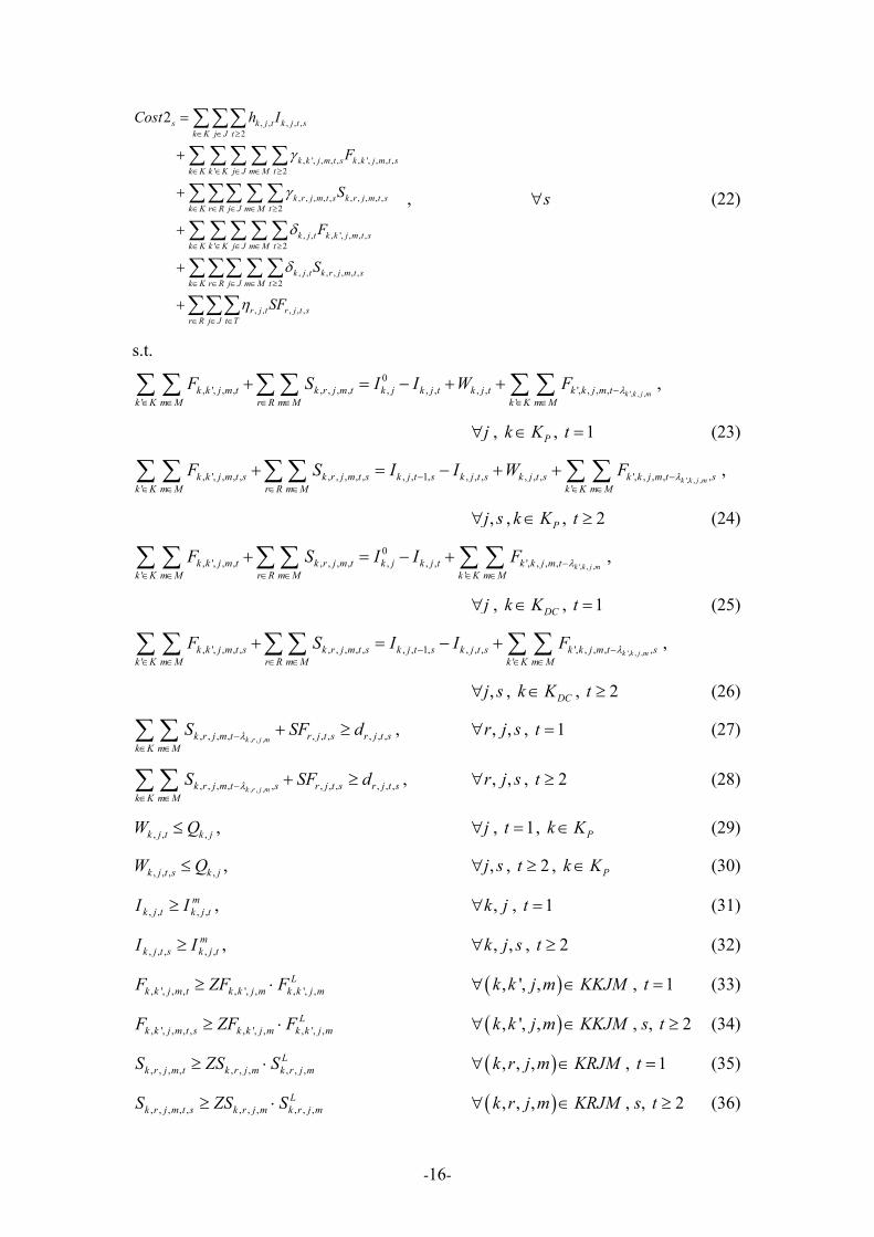
The objective function of this stochastic mixed-integer linear programming model

is to minimize the total expected cost given in (20), which includes the first-stage cost,

, and the expected second-stage cost. Since the scenarios follow discrete

distribution, the expected second-stage cost is equal to the product of the scenario

probability, , and the associated second-stage scenario cost, , summed over

all the scenarios s. Both the first-stage cost given in

1Cost

sp sCost2

(21) and the second-stage

scenario cost given in (22) are equal to the sum of the following items:

• Inventory holding cost for all products at all facilities for all time periods

• Freight cost for interfacility freight shipments in all the shipping lanes of all

the products in all time periods

• Freight cost for facility-customer shipments in all the shipping lanes of all the

products in all the time periods

• Facility throughput cost for interfacility shipments for all the shipping lanes of

all the products in all the time periods

• Facility throughput cost for facility-customer shipments for all the shipping

lanes of all the products in all the first-stage time periods

• Penalty costs of all the products for unmet demand of all the customers in all

the time periods

Six types of constraints are included in the model. The mass balance relationships

for the plants are given in constraints (23) and (24), the mass balance for distribution

centers are given in constraints (25) and (26), the demand balance for customers are

given in constraints (27) and (28), production capacity constraints are given in (29)

and (30), and minimum inventory level constraints are given in (31) and (32);

constraints (33)–(36) are minimum transportation level constraints for selected

transportation links/modes managed by third-party logistic companies. Constraints

(23), (25), (29), (31), (33), and (35) are first-stage constraints that do not include any

scenario-dependent (second-stage) variables, while the remaining constraints are

-17-

second-stage constraints for each scenario. The first-stage constraints are for the

production, inventory, and transportation planning of the first time period ( ),

except for the demand balance constraint

1t =

(27) that accounts for the uncertain demand

realization. Binary variables ZFk,k’,j,m and ZSk,r,j,m are introduced to model the semi-

continuous transportation levels for selected transportation links or modes. A slack

variable SFr,j,t,s is used to model the shortfalls and avoid infeasibility of the planning

problem. An additional feature of this model is that the transportation times are taken

into account through the multiperiod formulation and constraints (23)–(28), where

shipments across multiple time periods are explicitly taken into account.

Minimizing the objective function in (20)–(22), subject to the constraints in (23)–

(36), we can obtain the solution for the two-stage stochastic programming model.

Computational results for solving this model with the standard and the multicut

versions of the Benders decomposition method are presented in the next section.

4.3. Computational results

The problem is based on the global supply chain of a major commodity chemical

producer. We consider a planning horizon of one year, which is subdivided into 12

time periods, one month as a time period. Two products are produced and distributed

in the global supply chain. The customer demands and freight rates, which are

uncertain, follow normal distributions, with the forecast as the mean value and the

variance coming from the historical record. The demand uncertainty has three levels

of standard deviations. For the current month the standard deviation of demand is 5%

of the mean value; in the coming three months, the standard deviation is 10% of the

mean value; and for the remaining eight months, the demand has a standard deviation

of 20% of the mean value. Similarly, the freight rate has two levels of uncertainty. For

the current month, the variance is 0 (i.e., deterministic case); for the remaining 11

months, the freight rate has a standard deviation of 10% of the mean value. Three

makeup instances are considered, representing three supply chain networks. The first

instance is for a small network with 2 plants, 4 distribution centers, 2 customers, 1

transportation mode and 9 transportation links. The second instance is for a medium

size supply chain network with 5 plants, 17 distribution centers, 46 customers, 4

transportation modes and 75 transportation links. The third instance is for a large

network with 14 plants, 70 distribution centers, 126 customers, 14 transportation

-18-

modes, and 328 transportation links. Although the size of the stochastic programming

problem exponentially increases as the number of scenarios increases, we found that

at least 1,000 scenarios are required in order to achieve reasonable confidence

intervals. The problem sizes of the deterministic equivalents for three instances are

given in Table 3. All the instances are modeled with GAMS 23.4.3 and solved with

the CPLEX 12 solver on an IBM T400 laptop with an Intel Core Duo 2.53 GHz CPU

and 2 GB RAM. We note that none of these instances can be solved directly because

of their large size. Thus, the standard and multicut versions of the Benders

decomposition method are used. The optimality tolerances for both methods are set to

0.001%.

Table 3 Problem sizes of the deterministic equivalents for the example problem

Problem Size Instance 1 Instance 2 Instance 3 No. of Binary Variables 7 22 158 No. of Continuous Variables 423,036 3,703,384 75,356,014

No. of Constraints 201,018 1,301,789 52,684,187 The computational performances of the standard and multicut versions of the

Benders algorithm are shown in Figures 6 – 11. We can see that how the upper bound

decreases and the lower bound increases with the number of iterations, and how the

computational time increases for both solution methods in all these figures. For

Instance 1, the small-scale problem (results shown in Figures 6 and 7), the standard

Benders method requires 21 iterations (around 12 CPU-seconds) to converge, while

the multicut versions can reach the same optimality gap in 6 iterations (4 CPU-

seconds). Similarly, for Instance 2 with a medium-size supply chain network (results

shown in Figures 8 and 9), the multicut method requires only 45 iterations (around 5

CPU-minutes) to converge, while the standard Benders method takes 534 iterations

(around 45 CPU-minutes) to reach to the same optimality tolerance. As the problem

size becomes larger, the multicut Benders method is computationally much more

efficient than the standard method. For Instance 3, the largest problem (results shown

in Figures 10 and 11), the multicut version needs only 47 iterations (around 11 CPU-

minutes), while the standard Benders method requires 564 iterations (about 3.5 CPU-

hours).

The high computational efficiency of the multicut Benders method is because that

-19-

its master problem requiring relatively small solution times despite its large size, and

that the number of iterations is significantly reduced as a result of the “multiple” cuts.

In contrast, while the master problem in the standard Benders method is smaller in

size and faster to solve, it also requires a significantly larger number of iterations.

Note that both algorithms would benefit from solving the scenario subproblems with

parallel computing and coordinate through a master-worker computational framework

(Jeff Linderoth & Wright, 2003), which could significantly reduce the computational

times.

Figure 6 Comparison between the standard Benders method and the multicut

version in terms of number of iterations for the first instance of the global supply chain planning problem

-20-

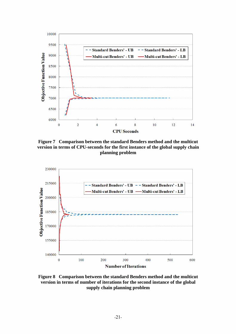
Figure 7 Comparison between the standard Benders method and the multicut version in terms of CPU-seconds for the first instance of the global supply chain

planning problem

Figure 8 Comparison between the standard Benders method and the multicut

version in terms of number of iterations for the second instance of the global supply chain planning problem

-21-

Figure 9 Comparison between the standard Benders method and the multicut

version in terms of CPU-seconds for the second instance of the global supply chain planning problem

Figure 10 Comparison between the standard Benders method and the multicut

version in terms of number of iterations for the third instance of the global supply chain planning problem

-22-

Figure 11 Comparison between the standard Benders method and the multicut version in terms of CPU-seconds for the third instance of the global supply chain

planning problem

5. Conclusion In this work, we described a multicut version of the Benders decomposition

method for the solution of two-stage stochastic programming problems. We discussed

the theory behind this algorithm and prove its convergence property. Two examples

were presented to illustrate the application of the proposed solution method. The first

example involves production-transportation planning under demand uncertainty. A

small example, for which the global optimal solution can be easily obtained by

solving its deterministic equivalent, was solved with both the standard and the

multicut versions of the Benders decomposition method. The results illustrated the

effectiveness of the multicut method. The second example involved a global chemical

supply chain planning under demand and freight rate uncertainty. The decomposition

method was tested on three large-scale instances, which cannot be solved directly

with a regular personal computer. Computational studies showed that although both

versions of the Benders decomposition method can solve large-scale stochastic

programming problems with reasonable computational effort, significant savings in

CPU time can be achieved by using the proposed multicut algorithm.

-23-

Acknowledgment We gratefully acknowledge financial support from the Dow Chemical Company,

the Pennsylvania Infrastructure Technology Alliance (PITA), the National Science

Foundation under Grant No. CMMI-0556090, and the U.S. Department of Energy

under contract DE-AC02-06CH11357.

Nomenclature for Section 3

Sets/Indices

I Set of production plants indexed by i

L Set of demand zones indexed by l

S Set of scenarios indexed by s

Decision Variables (values: 0 to +∞ )

[E profit] Total expected profit

iprod Production amount at plant i

,l ssale Total amount of the product sold to demand zone l of scenario s

,i lship Transportation amount from plant i to demand zone l

,l sunsold Unsold amount at demand zone l of scenario s

Parameters

icap Production capacity of plant i

icpd Unit production cost at plant i

,i lctr Unit transportation cost from plant i to demand zone l

lcus Unit unsold product cost in demand zone l

ldemand Demand in demand zone l of scenario s

,l sdemand Demand in demand zone l of scenario s

sp Probability of scenario s

lprice Sale price at demand zone l

-24-

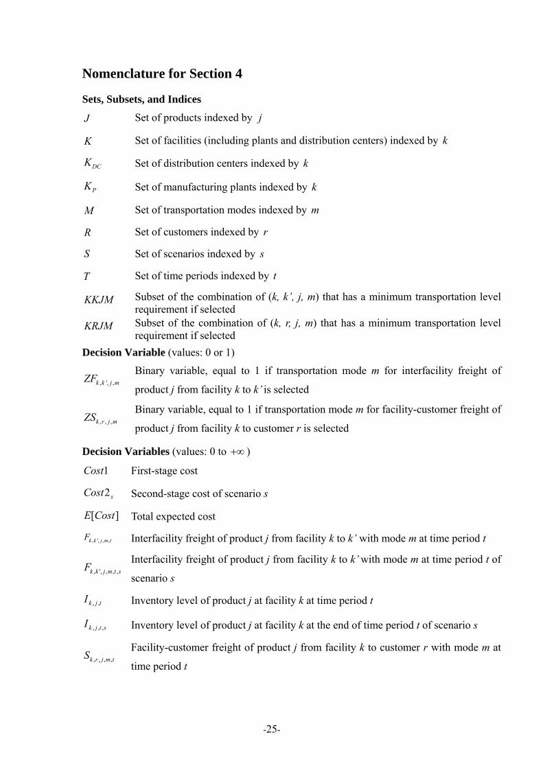
Nomenclature for Section 4

Sets, Subsets, and Indices

J Set of products indexed by j

K Set of facilities (including plants and distribution centers) indexed by k

DCK Set of distribution centers indexed by k

PK Set of manufacturing plants indexed by k

M Set of transportation modes indexed by m

R Set of customers indexed by r

S Set of scenarios indexed by s

T Set of time periods indexed by t

KKJM Subset of the combination of (k, k’, j, m) that has a minimum transportation level requirement if selected

KRJM Subset of the combination of (k, r, j, m) that has a minimum transportation level requirement if selected

Decision Variable (values: 0 or 1)

, ', ,k k j mZF Binary variable, equal to 1 if transportation mode m for interfacility freight of

product j from facility k to k’ is selected

, , ,k r j mZS Binary variable, equal to 1 if transportation mode m for facility-customer freight of

product j from facility k to customer r is selected

Decision Variables (values: 0 to +∞ )

1Cost First-stage cost

sCost2 Second-stage cost of scenario s

[E Cost] Total expected cost

, ', , ,k k j m tF Interfacility freight of product j from facility k to k’ with mode m at time period t

, ', , , ,k k j m t sF Interfacility freight of product j from facility k to k’ with mode m at time period t of

scenario s

tjkI ,, Inventory level of product j at facility k at time period t

stjkI ,,, Inventory level of product j at facility k at the end of time period t of scenario s

, , , ,k r j m tS Facility-customer freight of product j from facility k to customer r with mode m at

time period t

-25-

, , , , ,k r j m t sS Facility-customer freight of product j from facility k to customer r with mode m at

time period t of scenario s

stjrSF ,,, Unmet demand of product j in customer r at time period t of scenario s

, ,k j tW Production amount of product j at plant k at time period t, Pk K∈

, , ,k j t sW Production amount of product j at plant k at time period t of scenario s, Pk K∈

Parameters

stjrd ,,, Demand of product j in customer r at time period t of scenario s

, ,k j th Unit inventory cost of product j in facility k at time period t

, ', ,L

k k j mF Minimum transportation amount of product j from facility k to k’ with mode m at

each time period if this transportation link/mode is selected 0,k jI Initial inventory level of product j at facility k

mtjkI ,, Minimum inventory of product j at facility k at time period t

sp Probability of scenario s

,k jQ Capacity of plant k for product j, Pk K∈

, , ,Lk r j mS

Minimum transportation amount of product j from facility k to customer r with

mode m at each time period if this transportation link/mode is selected

, ', , ,k k m j tγ Freight rate of product j from facility k to k’ with mode m at time period t

, , , ,k r j m tγ Freight rate of product j from facility k to customer r with mode m at time period t

, ', , , ,k k j m t sγ Freight rate of product j from facility k to k’ with mode m at time t of scenario s

, , , , ,k r j m t sγ Freight rate of product j from facility k to customer r with mode m at time period t

of scenario s

, ,k j tδ Unit throughput cost of product j in facility k at time period t

, ,r j tη Unit penalty cost of product j for lost unmet demand in customer r at time period t

, ', ,k k j mλ Shipping time of product j from facility k to facility k’ with mode m

, , ,k r j mλ Shipping time of product j from facility k to customer r with mode m

-26-

References

Archibald, T. W., Buchanan, C. S., McKinnon, K. I. M., & Thomas, L. C. (1999). Nested Benders decomposition and dynamic programming for reservoir optimisation. Journal of the Operational Research Society, 50, 468-479.

Bahn, O., Dumerle, O., Goffin, J. L., & Vial, J. P. (1995). A cutting plane method from analytic centers for stochastic-programming. Mathematical Programming, 69, 45-73.

Benders, J. F. (1962). Partitioning procedures for solving mixed-variables programming problems. Numerische Mathematik, 4, 238–252.

Birge, J. R., & Louveaux, F. (1997). Introduction to Stochastic Programming. New York: Springer-Verlag.

Escudero, L. F., Garín, A., Merino, M., & Pérez, G. (2007). A two-stage stochastic integer programming approach as a mixture of branch-and-fix coordination and Benders decomposition schemes. Annals of Operations Research, 152, 395-420.

Fragniere, E., Gondzio, J., & Vial, J. P. (2000). Building and solving large-scale stochastic programs on an affordable distributed computing system. Annals of Operations Research, 99, 167-187.

Higle, J. L., & Sen, S. (1991). Stochastic decomposition - an algorithm for 2-stage linear-programs with recourse. Mathematics of Operations Research, 16, 650-669.

Infanger, G. (1993). Monte Carlo (importance) sampling within a Benders decomposition algorithm for stochastic linear programs. Annals of Operations Research, 39, 69-95.

Infanger, G. (1994). Planning under Uncertainty: Solving Large-Scale Stochastic Linear Programs. Danvers: Boyd and Fraser.

Latorre, J. M., Cerisola, S., Ramos, A., & Palacios, R. (2009). Analysis of stochastic problem decomposition algorithms in computational grids. Annals of Operations Research, 166 Issue: 1 Pages: Published: FEB 355-373.

Linderoth, J., Shapiro, A., & Wright, S. (2006). The empirical behavior of sampling methods for stochastic programming Annals of Operations Research, 142, 215-241.

Linderoth, J., & Wright, S. (2003). Decomposition Algorithms for Stochastic Programming on a Computational Grid. Computational Optimization and Applications, 24, 207–250.

Mulvey, J. M., & Ruszczynski, A. J. (1995). A new scenario decomposition method for large-scale stochastic optimization. Operations Research, 43, 477-490.

Ntaimo, L. (2010). Disjunctive Decomposition for Two-Stage Stochastic Mixed-Binary Programs with Random Recourse. Operations Research, 58, 229-243.

Rosenthal, R. E. (2010). GAMS- A User’s Manual: GAMS Development Corp. Ruszczynski, A. (1993). Parallel decomposition of multistage stochastic-programming

problems. Mathematical Programming, 58, 201-228. Ruszczyński, A. (1997). Decomposition methods in stochastic programming.

Mathematical Programming, 79, 333-353. Saharidis, G., & Ierapetritou, M. G. (2010). Improving benders decomposition using

maximum feasible subsystem (MFS) cut generation strategy. Computers & Chemical Engineering, 34, 1237.

-27-

-28-

Saharidis, G. K. D., Minoux, M., & Ierapetritou, M. G. (2010). Accelerating Bender's method using covering cut bundle generation. International Transactions in Operational Research, 17, 221.

Sen, S. (1993). Subgradient decomposition and differentiability of the recourse function of a 2-stage stochastic linear program. Operations Research Letters, 13, 143-148.

Sen, S., Zhou, Z., & Huang, K. (2009). Enhancements of two-stage stochastic decomposition. Computers & Operations Research, 36, 2434-2439.

Shapiro, A. (2000). Stochastic programming by Monte Carlo simulation methods. Stochastic Programming E-Prints Series, 03.

Shapiro, A. (2008). Stochastic programming approach to optimization under uncertainty. Mathematical Programming, 112, 183-220.

Shapiro, A., & Homem-de-Mello, T. (1998). A simulation-based approach to two-stage stochastic programming with recourse. Mathematical Programming, 81, 301-325.

Trukhanov, S., Ntaimo, L., & Schaefer, A. (2010). Adaptive multicut aggregation for two-stage stochastic linear programs with recourse. European Journal of Operational Research, 206, 395-406.

Van Slyke, R. M., & Wets, R. (1969). L-Shaped Linear Programs with Applications to Optimal Control and Stochastic Programming. SIAM Journal on Applied Mathematics, 17, 638-663.

Wassick, J. M. (2009). Enterprise-wide optimization in an integrated chemical complex. Computers & Chemical Engineering, 33, 1950-1963.

You, F., Wassick, J. M., & Grossmann, I. E. (2009). Risk management for global supply chain planning under uncertainty: models and algorithms. AIChE Journal, 55, 931-946.

The submitted manuscript has been created by UChicago Argonne, LLC, Operator of Argonne National Laboratory ("Argonne"). Argonne, a U.S. Department of Energy Office of Science laboratory, is operated under Contract No. DE-AC02-06CH11357. The U.S. Government retains for itself, and others acting on its behalf, a paid-up nonexclusive, irrevocable worldwide license in said article to reproduce, prepare derivative works, distribute copies to the public, and perform publicly and display publicly, by or on behalf of the Government.