Benders Decomposition - Technical University of Denmark · Thomas Stidsen 2 DTU-Management /...

1Thomas Stidsen

DTU-Management / Operations Research

Benders Decomposition– Using projections to solve problems

Thomas Stidsen

[email protected]

DTU-Management

Technical University of Denmark

2Thomas Stidsen


OutlineIntroduction

Using projections

Benders decomposition

Simple plant location example

Problems with Benders decompositionalgorithm

3Thomas Stidsen


Important readingsGood news: The only important readings from thislecture is:

Section 10.1

Section 10.2

Section 10.3

4Thomas Stidsen


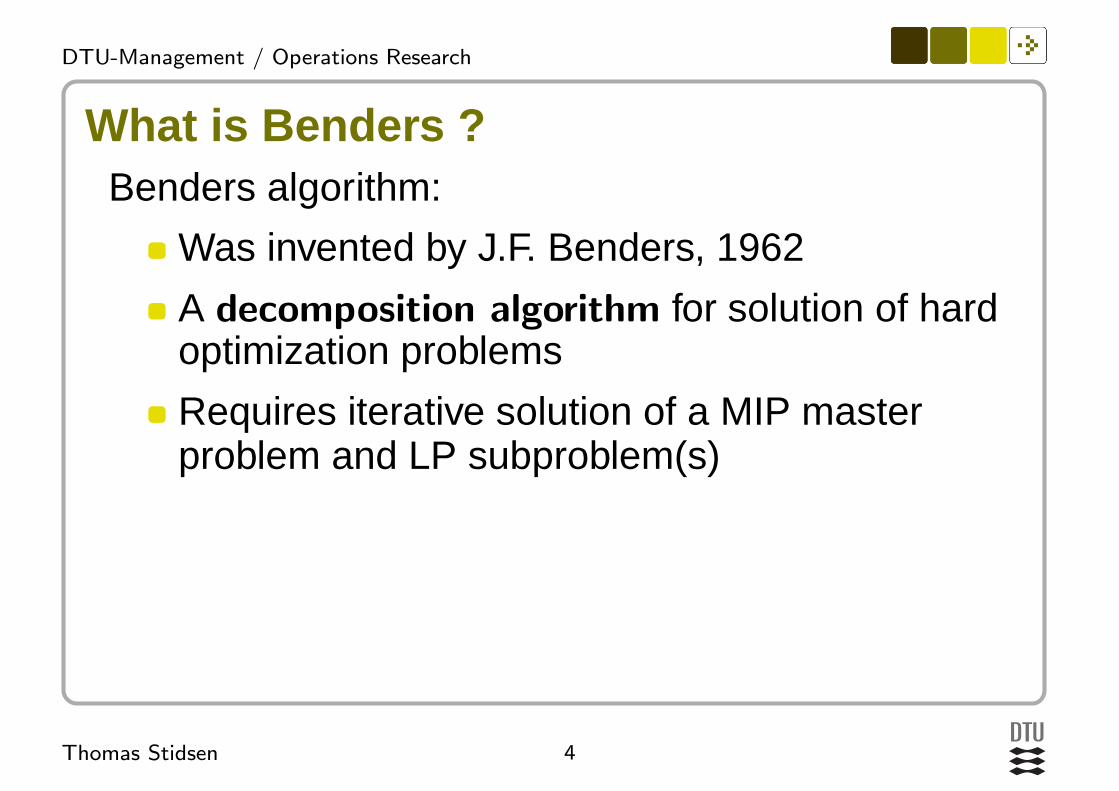
What is Benders ?Benders algorithm:

Was invented by J.F. Benders, 1962

A decomposition algorithm for solution of hardoptimization problems

Requires iterative solution of a MIP masterproblem and LP subproblem(s)

5Thomas Stidsen


Applying Projections

z0 ≥ dk uik k ∈ 1, . . . , q

0 ≥ dk uik k ∈ q + 1, . . . , r

bTuk = dk ∀k, Lemma 2.10

ATuk − c = 0 k ∈ 1, . . . , q, Lemma 2.10

ATuk = 0 k ∈ q + 1, . . . , r, Lemma 2.10

6Thomas Stidsen


The standard MIP ProblemMin

cTx + fTy

s.t.

Ax + By ≥ b

y ∈ Y

x ≥ 0

Notice: No assumption about y, but we will onlyconsider MIP problems, i.e. y ∈ Z

7Thomas Stidsen


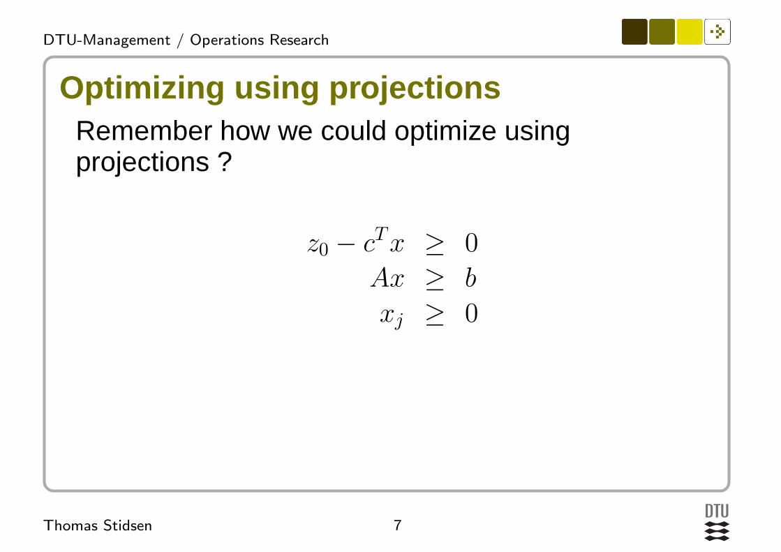
Optimizing using projectionsRemember how we could optimize usingprojections ?

z0 − cTx ≥ 0

Ax ≥ b

xj ≥ 0

8Thomas Stidsen


Re-arrangingMin

z0

s.t.

z0 − cTx ≥ fTy

Ax ≥ b − By

x ≥ 0 z ∈ R y ∈ Y

We make this rearrangement to enhance projection.

9Thomas Stidsen


Now we can project the x variables out !Min

z0

s.t.

ui0z0 ≥ ui

0fTy + (ui)T (b − By) i = 1, . . . , r

z ∈ R y ∈ Y

Notice that we only have one type of constraints(the two types are hidden in the possible values ofui

0, equal or not equal to zero).

10Thomas Stidsen


Rearrangeing projection resultsNow we re-scale with ui

0 (though not if ui0 = 0):

Min

z0

s.t.

z0 ≥ fTy + (ui)T (b − By) i = 1, . . . , q

0 ≥ (ui)T (b − By) i = q + 1, . . . , r

z ∈ R y ∈ Y

This is called Benders Master Program BMP(Notice: only y variables).

11Thomas Stidsen


But ...What did I tell you previously ? That the worstcasenumber of constraints is: (1

2)(2n+1−2)m2n

. This wasexactly the reason why we stated that the projectionmethod was not usefull in practice, so why bother ?Because we can generate the constraints on thefly. Big deal you may think, what if we still have togenerate all of them ?

12Thomas Stidsen


So ...We start with a problem with only a sub-set of thetwo types of constraints:

A subset of the optimization constraints

A subset of the feasibility constraints

Hence our restricted Benders Master Program is arelaxation of the full Benders Master Program.

13Thomas Stidsen


Hence ...If we optimize our restricted Benders MasterProgram and find the solution y, we may not havethe overall optimal solution because:

The solution may be too low (not optimal):zopt > z, because we need at least one moreoptimization constraint

The solution may be infeasible, because one ormore of the feasibility constraints in the fullBenders Master Program are missing.

14Thomas Stidsen


Benders Algorithm (Intuitively) (RKM 353)Start with a relaxed BMP with no constraints orjust a few of these. Solve the problem tooptimality getting the values y (or set initialvalues).

Given the values y we are also getting alowerbound zLO of the original problem.

Solve subproblem to get u, it may be:Infeasible (unbounded), generate ray u tofind the violated feasibility constraint ...Subproblem has a solution, find theconstraint such that fTy + (b − By)Tu > zLO

If the two bounds are sufficiently close, i.e.zUP − zLO ≤ ǫ, stop, otherwise iterate.

15Thomas Stidsen


Error in bookThere is an error in the algorithm on p. 353: Step 3,line 3 it says Bx in the feasibility cut, it should beBy.

16Thomas Stidsen


How to find the ui

We need to find the ui values to generate thefeasibility constraints and the optimality constraints.Given our problem:

Min

z0

s.t.

z0 ≥ fTy + (ui)T (b − By) i = 1, . . . , q

0 ≥ (ui)T (b − By) i = q + 1, . . . , r

z ∈ R y ∈ Y

17Thomas Stidsen


How to find the ui IIProp. 10.3 gives the ui as:

Extreme rays of {u|ATu ≤ 0, u ≥ 0}.

Extreme point of {u|ATu ≤ c, u ≥ 0} i.e.max{fTy + (b − By)Tu|ATu ≤ c, u ≥ 0}.

We will deal with the problem of extreme rays to thelecture next week.

18Thomas Stidsen


The Subproblem (called: Primal subproblem)Thus we have to find the extreme points u given aset of fixed values y:

Max

fTy + (b − By)Tu

s.t.

ATu ≤ c

u ≥ 0

19Thomas Stidsen


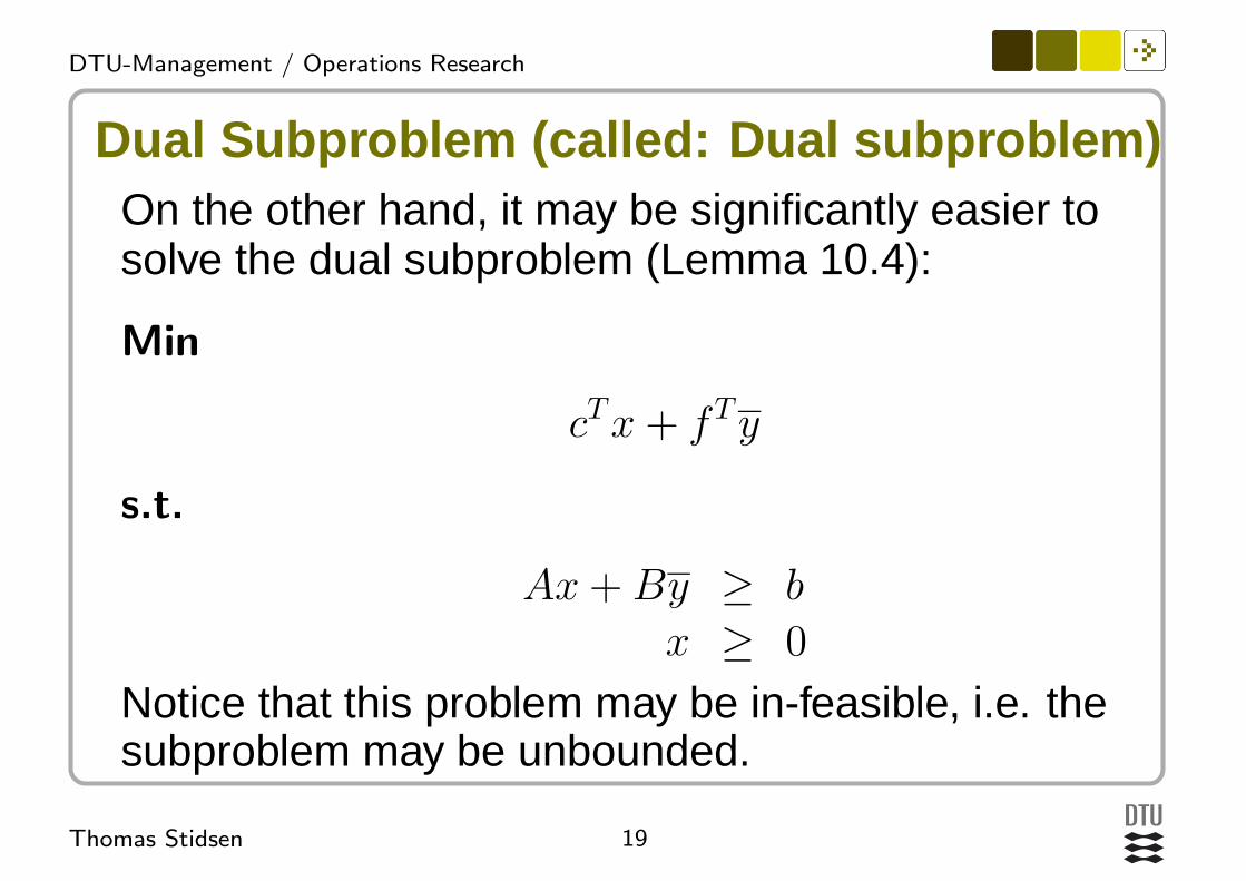
Dual Subproblem (called: Dual subproblem)On the other hand, it may be significantly easier tosolve the dual subproblem (Lemma 10.4):

Min

cTx + fTy

s.t.

Ax + By ≥ b

x ≥ 0

Notice that this problem may be in-feasible, i.e. thesubproblem may be unbounded.

20Thomas Stidsen


Dual Subproblem IIWhat is the dual subproblem ??? It is simply theprimal subproblem where the y are fixed !

This makes the dual subproblem an easyversion of the original problem, because the“hard” variables are fixed.

We can use a standard LP solver to solve theproblem.

There is absolutely nothing wrong in solving theprimal subproblem instead, but then you first haveto dualize the problem !

21Thomas Stidsen


Upper and Lower bounds

Iteration

Unknown optimum

Epsilon

Objective to be minimised

Lowerbounds

Upperbounds/solutions

22Thomas Stidsen


Section (10.3): Simple Facility LocationWe will now look at the example in section 10.3.This example you should study in detail !minimise:

∑

i

∑

j

ci,j · xi,j +∑

i

fi · yi

s.t.∑

i

xi,j ≥ 1 j = 1, . . . m

−xi,j + yi ≥ 0 i = 1, . . . n, j = 1, . . . m

xi,j ≥ 0 yi ∈ {0, 1}

23Thomas Stidsen


The (dual) subproblemGiven a choice of facility locations y, O(i) are theopen facilities and C(i) are the closed facilities.minimise:

∑

i

∑

j

ci,j · xi,j +∑

i∈O(y)

fi

s.t.∑

i

xi,j ≥ 1 j = 1, . . . m

xi,j ≤ 1 i = 1 ∈ O(y)

xi,j ≤ 0 i = 1 ∈ C(y)

xi,j ≥ 0

24Thomas Stidsen


Example 10.6: The dataTable 10.1, p. 355 RKM:

1 2 3 4 5 fixed costs1 2 3 4 5 7 2

Plant 2 4 3 1 2 6 33 5 4 2 1 3 3

25Thomas Stidsen


Example 10.6: The matrixesUnfortunately it is necessary to fully describe thematrixes for the problem in a form corresponding tothe formulas (10.1) - (10.4). This is necessary inorder to be able to calculate the optimality andfeasiblilty cuts.

26Thomas Stidsen


Example 10.6: The A matrix

A =

2

6

6

6

6

6

6

6

6

6

6

6

6

6

6

6

6

6

6

6

6

6

6

6

6

6

6

6

6

6

6

6

6

6

6

6

6

6

6

6

6

6

6

6

1 1 1

1 1 1

1 1 1

1 1 1

1 1 1

-1

-1

-1

-1

-1

-1

-1

-1

-1

-1

-1

3

7

7

7

7

7

7

7

7

7

7

7

7

7

7

7

7

7

7

7

7

7

7

7

7

7

7

7

7

7

7

7

7

7

7

7

7

7

7

7

7

7

7

7

27Thomas Stidsen


Example 10.6: The B matrix

B =

2

6

6

6

6

6

6

6

6

6

6

6

6

6

6

6

6

6

6

6

6

6

6

6

6

6

6

6

6

6

6

6

6

6

6

6

6

6

6

6

6

6

6

6

1

1

1

1

1

1

1

1

1

1

1

3

7

7

7

7

7

7

7

7

7

7

7

7

7

7

7

7

7

7

7

7

7

7

7

7

7

7

7

7

7

7

7

7

7

7

7

7

7

7

7

7

7

7

7

28Thomas Stidsen


Example 10.6: The b, c and d vectorsbT = [1, 1, 1, 1, 1, 0, 0, 0, 0, 0, 0, 0, 0, 0, 0, 0, 0, 0, 0, 0]

cT = [2, 3, 4, 5, 7, 4, 3, 1, 2, 6, 5, 4, 2, 1, 3]

fT = [2, 3, 3]

29Thomas Stidsen


Example 10.61. iteration, subproblem, with:y1 = 1, y2 = 0, y3 = 0, gives the solution: x1j = 1 andan upper bound zUP = 23. Since the lower bound iszLO = −∞ we cannot terminate.

30Thomas Stidsen


Example 10.6How to get the bounding constraints. Observe that:

If∑

i yi ≥ 1 the solution to the dual subproblemis always feasible, i.e. the primal subproblem isnever unbounded (extreme rays). Hence, giventhis restriction we will never have to addfeasibility cuts.

We need to get a way to construct the optimalityconstraints for the BMP

31Thomas Stidsen


Example 10.6Finally, lets get to the optimality cuts, in general:

z0 ≥ uT (b − By) + fTy

We need the u values. We can get these, either us-

ing an LP solver or by hand calculations ...

32Thomas Stidsen


Example 10.6: “Hand” calculation of duals vj

u = [v, w] where v are the demand duals and w arethe open/closed facility duals.

The dual variables vj for the demandconstraints have the value: vj = mini∈O(y){cij},i.e. equal to the cost from the “closest” openfacility.

33Thomas Stidsen


Example 10.6: “Hand” calculation of duals wij

The dual variables wij corresponding to theopen and closed facilities:

wij = 0, i ∈ O(y), because adding morecapacity to an already open plant will notchange the cost of a solution.wij = maxi∈C(y){(vj − cij), 0}. It can nevercost, besides the fixed costs fi to open afacility, hence it is always greater or equal tozero. The most we can gain by opening afacility is the difference between the currentcost vj and the cost if this i’th was availablecij.

34Thomas Stidsen


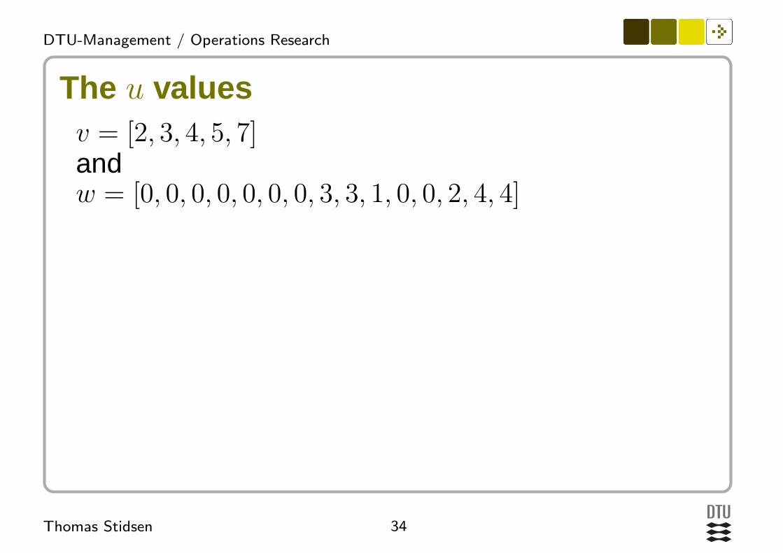
The u valuesv = [2, 3, 4, 5, 7]andw = [0, 0, 0, 0, 0, 0, 0, 3, 3, 1, 0, 0, 2, 4, 4]

35Thomas Stidsen


The u valuesbut given the above dual variables vj and wij:

z0 ≥

5∑

j=1

vj +3∑

i=1

(fi − ρi)yi

where:ρi =

∑5j=1 wij

36Thomas Stidsen


The u valuesHence:ρ1 = 0 + 0 + 0 + 0 + 0 = 0, i.e. (f1 − ρ1) = 2 − 0 = 2ρ2 = 0, 0, 3, 3, 1 = 7, i.e. (f2 − ρ2) = 3 − 7 = −4ρ3 = 0, 0, 2, 4, 4 = 10, i.e. (f2 − ρ3) = 3 − 10 = −7Hence:z0 ≥ 21 + 2y1 − 4y2 − 7y3

37Thomas Stidsen


Example 10.6Given the solution to the first dual subproblem:x11 = x12 = x13 = x14 = x15 = 1with the optimal value UB = 23.But what we really need is the u variables which arethe dual variables for the dual subproblem !

38Thomas Stidsen


Example 10.6The first BMP becomes:

minimise:

z0

s.t.

z0 ≥ 21 + 2y1 − 4y2 − 7y3

y1 + y2 + y3 ≥ 1

yi ∈ {0, 1}

39Thomas Stidsen


Example 10.6Giving the optimal solution:y1 = 0, y2 = 1, y3 = 1 and z0 = 10 and henceLO = max(−∞, 10). Because we have UB = 23(from the dual subproblem) we decide thatUB − LO = 13 is too much, and we continue ...

40Thomas Stidsen


Questions:There are a number of interesting questions whichmay be raised:

How many iterations needs to be performed ?

A related question: How many constraints arebinding for the optimal solution ?

The quote: “For the Benders decompositionalgorithm to be effective it is essential that thelinear programming subproblem have specialstructure so that it is easily optimized”, p. 357.This is in my view wrong. The real problem issolving the BMP !

41Thomas Stidsen


Number of iterationsThe number of iterations is critical and we cannotgive any guarantees, why ? We may have togenerate all extreme rays, and this number may beexponential (corner points ATu ≤ c).

Benders Decomposition - Technical University of Denmark · Thomas Stidsen 2 DTU-Management /...

Documents

Transcript of Benders Decomposition - Technical University of Denmark · Thomas Stidsen 2 DTU-Management /...