Multi-Objective Monte Carlo Tree Search for Real-Time...

IEEE TRANSACTIONS ON COMPUTATIONAL INTELLIGENCE AND AI IN GAMES 1

Multi-Objective Monte Carlo Tree Search for Real-Time GamesDiego Perez, Student Member, IEEE, Sanaz Mostaghim, Member, IEEE, Spyridon Samothrakis, Student Member,

IEEE, Simon M. Lucas, Senior Member, IEEE

Abstract—Multi-objective optimization has been traditionallya matter of study in domains like engineering or finance, withlittle impact on games research. However, action-decision basedon multi-objective evaluation may be beneficial in order to obtaina high quality level of play. This paper presents a Multi-objectiveMonte Carlo Tree Search algorithm for planning and control inreal-time game domains, those where the time budget to decidethe next move to make is close to 40ms. A comparison is madebetween the proposed algorithm, a single-objective version ofMonte Carlo Tree Search and a rolling horizon implementationof Non-dominated Sorting Evolutionary Algorithm II (NSGA-II).Two different benchmarks are employed, Deep Sea Treasure andthe Multi-Objective Physical Travelling Salesman Problem. Usingthe same heuristics on each game, the analysis is focused on howwell the algorithms explore the search space. Results show thatthe algorithm proposed outperforms NSGA-II. Additionally, it isalso shown that the algorithm is able to converge to differentoptimal solutions or the optimal Pareto front (if achieved duringsearch).

I. INTRODUCTION

Multi-objective optimization has been a field of study inmanufacturing, engineering [1] and finance [2], while havinglittle impact on games research. This paper shows that multi-objective optimization has much to offer in developing gamestrategies that allow for a fine-grained control of alternativepolicies. The application of such approaches to this field canprovide interesting results, especially in games that are longor complex enough that long-term planning is not trivial, andachieving a good level of play requires balancing strategies.

At their most basic, many competitive games can be viewedas simply two or more opponents having the single objective ofwinning. Achieving victory is usually complex in interestinggames, and successful approaches normally assign some formof value to a state, value being long term expected reward(i.e. expectation of victory). Due to a massive search space,heuristics are often used for this value function. An exampleis a chess heuristic that assigns different weights to each pieceaccording to an estimated value.

Multi-objective approaches can be applied to scenarioswhere several factors must be taken into account to achievevictory. The algorithms can balance between different objec-tives, in order to provide a wide range of strategies well suitedto the different stages of the game being played, or to faceexisting opponents. Application of such approaches could bereal-time strategy games, where long term planning must be

Diego Perez, Spyridon Samothrakis, Simon M. Lucas (School of ComputerScience and Electronic Engineering, University of Essex, Colchester CO43SQ, UK; email: dperez,ssamot,[email protected]);Sanaz Mostaghim (Department of Knowledge and Language Engineer-ing, Otto-von-Guericke-Universitt Magdeburg, Magdeburg, Germany; email:[email protected])

carried out in order to balance aspects such as attack units,defensive structures and resource gathering. This should allowsmart balancing of heuristics.

This paper proposes a multi-objective real-time algorithmversion of Monte Carlo Tree Search (MCTS), a popular rein-forcement learning approach that emerged in the last decade.The proposed algorithm is tested in two different games: areal-time version of the Deep Sea Treasure (DST; a classicalmulti-objective problem), and the Multi-Objective PhysicalTravelling Salesman Problem (MO-PTSP). The algorithm isalso compared with another two approaches: a single-objectiveMCTS (that uses a weighted sum of features to value the state)and a rolling horizon Non-dominated Sorting EvolutionaryAlgorithm II (NSGA-II). This paper extends and formalizesour previous work described in [3].

Two main goals can be identified in this paper: first, theproposed algorithm must be applicable to real-time domains(those where the next move to make must be decided withina small time budget) and it should obtain better or at least thesame performance than the other algorithms. It is importantto highlight that all three algorithms tested employ the sameheuristic functions to evaluate the features of a given gamestate. Thus, the focus of this research is set on how thealgorithm explores the search space, instead of providing thebest possible solution to each given problem.

Secondly, the algorithm must be able to provide solutionsacross the multi-objective spectrum: by parametrizing thealgorithm, it must be possible to prioritize one objective overthe others and therefore converge to solutions according tothese preferences. Therefore, the main contribution of thispaper is the proposal of a multi-objective version of MCTSthat is applicable to real-time domains and is able to providedifferent solutions across the multi-objective spectrum.

The paper is structured as follows. First, Sections II and IIIprovide the necessary background for MCTS and multi-objective optimization, respectively. The algorithm proposedin this research is described in detail in Section IV. Then,Section V defines the games used to test the algorithms, withthe results discussed in Section VI. Finally, some conclusionsand possible extensions of this work are drawn in Section VII.

II. MONTE CARLO TREE SEARCH

Monte Carlo Tree Search (MCTS) is a tree search algorithmthat was originally applied to board games, gaining momentumand popularity in the game of Go. This game is played ina square grid board, with a size of 19 × 19 in the originalgame, and 9×9 in its reduced version. The game is played inturns, and the objective is to surround the opponent’s stones


Fig. 1: MCTS algorithm steps.

by placing stones in any available position on the board. Dueto the very large branching factor of the game and the absenceof clear heuristics to tackle it, Go became object of study formany researchers. MCTS was the first algorithm able to reachprofessional level play in the reduced board size version [4].After its success in Go, MCTS has been used extensively bymany researchers in this and different domains. An extensivesurvey of MCTS methods, variations and applications, hasbeen written by Browne et al. [5].

MCTS is considered to be an anytime algorithm, as it isable to provide a valid next move to choose at any momentin time. This is true independently from how many iterationsthe algorithm is able to make (although, in general, more iter-ations usually produce better results). This differs from otheralgorithms (such as A* in single player games, and standardMin-Max for two player games) that normally provide thenext play only after they have finished. This makes MCTS asuitable candidate for real-time domains, where the decisiontime budget is limited, affecting the number of iterations thatcan be performed.

MCTS is an algorithm that builds a tree in memory. Eachnode in the tree maintains statistics that indicate how often amove is played from a given state (N(s, a)), how many timeseach move is played from there (N(s)) and the average reward(Q(s, a)) obtained after applying move a in state s. The treeis built iteratively by simulating actions in the game, makingmove choices based on statistics stored in the nodes.

Each iteration of MCTS can be divided into several steps,as introduced by G. Chaslot et al. [6]: Tree selection, Ex-pansion, Monte Carlo simulation and Back-propagation (allsummarized in Figure 1). When the algorithm starts, the treeis formed only by the root node, which holds the current stateof the game. During the selection step, the tree is navigatedfrom the root until a maximum depth or the end of the gamehas been reached.

In every one of these action decisions, MCTS balances be-tween exploitation and exploration. In other words, it choosesbetween taking an action that leads to states with the bestoutcome found so far, and performing a move to go to lessexplored game states, respectively. In order to achieve this,Kocsis and Szepesvari [7] applied Upper Confidence Bound(UCB1, see Equation 1) as a Tree Policy.

a∗ = arg maxa∈A(s)

Q(s, a) + C

√lnN(s)

N(s, a)

(1)

The balance between exploration and exploitation can betempered by modifying C. Higher values of C give addedweight to the second term of the UCB1 Equation 1, givingpreference to those actions that have been explored less, atthe expense of taking actions with the highest average rewardQ(s, a). A commonly used value for single-player gamesis√

2, as it balances both facets of the search when therewards are normalized between 0 and 1. The value of C isapplication dependant, and it may vary from game to game.It is worth noting that MCTS, when combined with UCB1,reaches asymptotically logarithmic regret on each node of thetree [8].

If, during the tree selection phase, a node has fewer childrenthan the available number of actions from a given position, anew node is added as a child of the current one (expansionphase) and the simulation step starts. At this point, MCTSexecutes a Monte Carlo simulation (or roll-out; default policy)from the expanded node. This is performed by choosingrandom (either uniformly random, or biased) actions until thegame end or a pre-defined depth is reached, where the stateof the game is evaluated.

Finally, during the back-propagation step, the statisticsN(s), N(s, a) and Q(s, a) are updated for each node visited,using the reward obtained in the evaluation of the state. Thesesteps are executed in a loop until a termination criteria is met(such as number of iterations).

MCTS has been employed extensively in real-time games.An example of this is the popular real-time game Ms. PacMan.The objective of this game is to control Ms. PacMan to clearthe maze by eating all pills, without being captured by theghosts. An important feature of this game is that it is open-ended, as an end game situation is, most of the time, far aheadin the future and can not be devised by the algorithm duringits iterations. The consequence of this is that MCTS, in itsvanilla form, it is not able to know if a given ply will lead toa win or a loss in the end game state. Robles et al. [9] solvedthis problem by including hand-coded heuristics that guidedsearch towards more promising portions of the search space.This approach enabled the addition of heuristics knowledge toMCTS, as in [10], [11].

MCTS has also been applied to single-player games, likeSameGame [12], where the player’s goal is to destroy con-tiguous tiles of the same colour, distributed in a rectangulargrid. Another use of MCTS is in the popular puzzle MorpionSolitaire [13], a connection game where the goal is to linknodes of a graph with straight lines that must contain at leastfive vertices. Finally, the PTSP has also been addressed byMCTS, both in the single-objective [14], [15] and the multi-objective versions [16]. These papers describe the entries thatwon both editions of the PTSP Competition.

It is worthwhile mentioning that in most cases found in theliterature, MCTS techniques have been used with some kindof heuristic that guides the Monte Carlo simulations or thetree selection policy. In the algorithm proposed in this paper,


Fig. 2: Decision and objective spaces in a MOP with twovariables (x1 and x2) and two objectives (f1 and f2). In theobjective space, yellow dots are non-optimal objective vectors,while blue dots form a non-dominated set. From [17].

simulations are purely random, as the objective is to comparethe search abilities of the different algorithms. The intention istherefore to keep the heuristics to a minimum, and the existingpieces of domain knowledge are shared by all the algorithmspresented (as in the case of the score function for MO-PTSP,described later).

III. MULTI-OBJECTIVE OPTIMIZATION

A multi-objective optimization problem (MOP) representsa scenario where two or more conflicting objective functionsare to be optimized at the same time and is defined as:

optimize f1(~x), f2(~x), · · · , fm(~x) (2)

subject to ~x ∈ Ω, involving m(≥ 2) conflicting objec-tive functions fi : <n → <. The decision vectors ~x =(x1, x2, · · · , xn)T belong to the feasible region Ω ⊂ <n. Wedenote the image of the feasible region by Z ⊂ <m and callit a feasible objective region. The elements of Z are calledobjective vectors and they consist of m objective (function)values ~f(~x) = (f1(~x), f2(~x), · · · , fm(~x)). Therefore, eachsolution ~x provides m different scores (or rewards, or fitness)that are meant to be optimized. Without loss of generality, it isassumed from now on that all objectives are to be maximized.

It is said that a solution ~x dominates another solution ~y ifand only if:

1) fi(~x) is not worse than fi(~y), ∀i = 1, 2, . . . ,m.2) For at least one objective j: fj(~x) is better than its

analogous counterpart in fj(~y).When these two conditions apply, it is said that ~x ~y

(~x dominates ~y). The dominance condition provides a partialordering between solutions in the objective space.

However, there are some cases where it cannot be said that~x ~y or ~y ~x. In this case, it is said that these solutions areindifferent to each other. Solutions that are not dominated canbe grouped in a non-dominated set. Given a non-dominatedset P , it is said that P is the Pareto-set if there is no othersolution in the decision space that dominates any memberof P . The corresponding objective vectors of the membersin the Pareto-set build a so called Pareto-front. The relationsbetween decision and objective space, dominance and the non-dominated set are depicted in Figure 2.

There are many different algorithms in the literature that areproposed to tackle multi-objective optimization problems [18].

Algorithm 1 NSGA-II Algorithm [21]1: Input: MOP, N2: Output: Non-dominated Set F0

3: t = 04: Pop(t) = NewRandomPopulation5: Q(t) = breed(Pop(t)) % Generate offspring6: while Termination criterion not met do7: U(t) = Pop(t) ∪Q(t)8: F = FASTNONDOMINATEDSORT(U(t))9: Pop(t+ 1) = ∅, i = 0

10: while |Pop(t+ 1)|+ |Fi| ≤ N do11: CROWDINGDISTANCEASSIGNMENT(Fi)12: Pop(t+ 1) = Pop(t+ 1) ∪ Fi

13: i = i+ 1

14: SORT(Pop(t+ 1))15: Pop(t+ 1) = Pop(t+ 1)∪Fi[1 : (N −|Pop(t+ 1)|)]16: Q(t+ 1) = breed(Pop(t+ 1))17: t = t+ 1

return F0

A weighted-sum approach is one of the traditional methods inwhich the objectives are weighted according to user prefer-ence. The sum of the weighted objectives builds one objectivefunction to be optimized. The solution to this single-objectiveproblem is one certain solution, ideally on a Pareto-front. Byvarying the weights, it is possible to converge to differentoptimal solutions. Such linear scalarization approaches failto find optimal solutions for problems with non-convex-shapePareto-fronts [18].

A popular choice for multi-objective optimization prob-lems are evolutionary multi-objective optimization (EMO)algorithms [19], [20]. The goal of EMO algorithms is to finda set of optimal solutions with a good convergence to thePareto-front as well as a good spread and diversity alongthe Pareto-front. One of the most well-known algorithmsin the literature is the Non-dominated Sorting EvolutionaryAlgorithm II (NSGA-II) [21], the pseudocode of which isshown in Algorithm 1. NSGA-II is known to deliver solutionswith very good diversity and convergence to the Pareto-frontfor 2-objective problems. However, for problems with morethan 3 objectives, other approaches such as NSGA-III [22],SMS-EMOA [23] and MOEA/D [24] are shown to outperformNSGA-II. As in any evolutionary algorithm, NSGA-II evolvesa set of N individuals in a population denoted as Pop withthe difference that they are ranked according to a dominancecriterion and a crowding distance measure, which are used tomaintain a good diversity of solutions. After each iteration ofthe algorithm, only the best N individuals according to thisranking are maintained to the next generation.

The three main pillars of the NSGA-II algorithm are:• Fast non-dominated sorting: The function F =

FASTNONDOMINATEDSORT(U(t)) performs a non-dominated sorting and ranks the individuals stored in aset U into several non-dominated fronts denoted as Fi,where the solutions in F0 are the non-dominated solutionsin the entire set. Fi is the set of non-dominated solutionsin R \ (F0 ∪ · · · ∪ Fi−1).


• Crowding distance: The functionCROWDINGDISTANCEASSIGNMENT(Fi) assigns toeach one of the individuals in Fi a crowding distancevalue, which is the distance between the individualand its neighbours. The individuals with the smallestcrowding distances are selected with a lower probabilitythan the ones with larger values.

• Elitism: The individuals from the first front F0 are alwaysranked first, according to the dominance criterion andtheir crowding distance.

For more details about EMO approaches, please refer to[18].

A. Multi-objective Reinforcement Learning (MORL)

Reinforcement Learning (RL) algorithms have also beenused with MOPs. RL [25] is a broad field in Machine Learningthat studies real-time planning and control situations where anagent has to find the actions (or sequences of actions) thatshould be used in order to maximize the reward from theenvironment.

The dynamics of an RL problem are usually captured by aMarkov Decision Process (MDP) which is a tuple (S,A, T,R),in which S is the set of possible states in the problem (orgame), and s0 is the initial state. A is the set of availableactions the agent can make at any given time, and the transitionmodel T (si, ai, si+1) determines the probability of reachingthe state si+1 when action ai is applied in state si. Thereward function R(si) provides a single value (reward) thatthe agent must optimize, representing the desirability of thestate si reached. Finally, a policy π(si) = ai determines whichactions ai must be chosen from each state si ∈ S1. One ofthe most important challenges in RL, as shown in Section II,is the trade-off between exploration and exploitation whiletrying to act. While learning, a policy must choose betweenselecting the actions that provided good rewards in the pastand exploring new parts of the search space by selecting newactions.

Multi-objective Reinforcement Learning (MORL) [26]changes this definition by using a vector R = r1, . . . , rm asrewards of the problem (instead of a scalar). Thus, MORLproblems differ from RL in having more than one objective(here m) that must be maximized. If the objectives areindependent or non-conflicting, scalarization approaches suchas the weighted sum approach, could be suitable to tackle theproblem. Essentially, this would mean using a conventionalRL algorithm on a single objective where the global rewardis obtained from a weighted-sum of the multiple rewards.However, this is not always the case, as usually the objectivesare conflicting and the policy π must balance among them.

Vamplew et al. [26] propose a single-policy algorithm whichuses a preference order in the objectives (either given by theuser or by the nature of the problem). An example of this typeof algorithm can be found at [27], where the authors introducean order of preference in the objectives and constrain the valueof the desired rewards. Scalarization approaches would also

1This is a deterministic policy and only valid during acting, not learning

Fig. 3: HV (P ) of a given Pareto-front P

fit in this category, as shown in the work performed by S.Natarajan et al. [28].

The second type of algorithms, multiple-policy, aims toapproximate the optimal Pareto-front of the problem. This isthe aim of the algorithm proposed in this paper. An example ofthis type of algorithm is the one given by L. Barrett [29], whoproposes the Convex Hull Iteration Algorithm. This algorithmprovides the optimal policy for any linear preference function,by learning all policies that define the convex hull of thePareto-front.

B. Metrics

The quality of an obtained non-dominated set can bemeasured using different diversity or/and convergence met-rics [18]. The Hypervolume Indicator (HV) is a popular metricfor measuring both the diversity and convergence of non-dominated solutions [30]. This approach can be additionallyused to compare different non-dominated sets. Given a Paretofront P , HV (P ) is defined as the volume of the objectivespace dominated by P . More formally, HV (P ) = µ(x ∈ Rd :∃r ∈ P s.t r x), where µ is the de Lebesgue measureon Rd. If the objectives are to be maximized, the higher theHV (P ), the better the front calculated. Figure 3 shows anexample of HV (P ) where the objective dimension space ism = 2.

IV. MULTI-OBJECTIVE MONTE CARLO TREE SEARCH

Adapting MCTS into Multi-Objective Monte Carlo TreeSearch (MO-MCTS) requires the obvious modification ofdealing with multiple rewards instead of just one. As theseare collected at the end of a Monte Carlo simulation, thereward value r now becomes a vector R = r0, r1, . . . , rm,where m is the number of objectives to optimize. Derivedfrom this change, the average value Q(s, a) becomes a vectorthat stores the average reward of each objective. Note that theother statistics (N(s, a) and N(s)) do not need to change, asthese are just node and action counters. The important questionto answer next is how to adapt the vector Q(s, a) to use it inthe UCB1 formula (Equation 1).

An initial attempt at Multi-Objective MCTS was addressedby W. Wang and Michele Sebag [31], [32]. In their work, the


Fig. 4: rpx is the projection of the rx value on the piecewiselinear surface (discontinuous line). The shadowed surfacerepresents HV (P ). From [31].

authors employ a mechanism, based on the HV calculation,to replace the UCB1 equation. The algorithm keeps a Paretoarchive (P) with the best solutions found in end game states.Every node in the tree defines rsa as a vector of UCB1 values,in which each rsa,i is the result of calculating UCB1 for eachparticular objective i.

The next step is to define the value for each state and actionpair, V (s, a), as in Equation 3. rpsa is the projection of rsa intothe piecewise linear surface defined by the Pareto archive P(see Figure 4). Then, HV (P ∪ rsa) is declared as the HV ofP plus the point rsa. If rsa is dominated by P, the distancebetween rsa and rpsa is subtracted from the HV calculation.The tree policy selects actions based on a maximization of thevalue of V (s, a).

V (s, a) =

HV (P ∪ rsa)− dist(rpsa, rsa) OtherwiseHV (P ∪ rsa) if rsa P

(3)The proposed algorithm was employed successfully in two

domains: the DST and the Grid Scheduling problem. In bothcases, the results matched the state-of-the-art, albeit at theexpense of a high computational cost.

As mentioned before, one of the objectives of this paper isto propose an MO-MCTS algorithm that is suitable for real-time domains. Therefore, an approach different from Wang’sis needed, in order to overcome the high computational costinvolved in their approach.

In the algorithm proposed in this paper, the reward vectorr that was obtained at the end of a Monte Carlo simulation isback-propagated through the nodes visited in the last iterationuntil the root is reached. In the vanilla algorithm, each nodewould use this vector r to update its own accumulated rewardvector R. In the algorithm proposed here, each node inthe MO-MCTS algorithm also keeps a local Pareto frontapproximation (P ), updated at each iteration with the rewardvector r obtained at the end of the simulation. Algorithm 2describes how the node statistics are updated in MO-MCTS.

Here, if r is not dominated by the local Pareto frontapproximation, it is added to the front and r is propagated

Algorithm 2 Pareto MO-MCTS node update.1: function UPDATE(node, r, dominated = false)2: node.V isits = node.V isits+ 13: node.R = node.R+ r4: if !dominated then5: if node.P r then6: dominated = true7: else8: node.P = node.P ∪ r9: UPDATE(node.parent, r, dominated)

to its parent. It may also happen that r dominates all orsome solutions of the local front, in which case the newsolution is included and the dominated solutions are removedfrom the Pareto front approximation. If r is dominated bythe node’s Pareto front approximation, it does not change andthere is no need to maintain this propagation up the tree. Threeobservations can be made about the mechanism described here:

• Each node in the tree has an estimate of the quality ofthe solutions reachable from there, both as an average (asin the baseline MCTS) and as the best case scenario (bykeeping the non-dominated front P ).

• By construction, if a reward r is dominated by the localfront of a node, it is a given that it will be dominated bythe nodes above in the tree, so there is no need to updatethe fronts of the upper nodes, producing little impact onthe computational cost of the algorithm.

• It is easy to infer, from the last point, that the Pareto frontapproximation of a node cannot be worse than the frontof its children (in other words, the front of a child willnever dominate that of its parent). Therefore, the root ofthe tree contains the best non-dominated front ever foundduring the search.

This last detail is important for two main reasons. Firstof all, the algorithm allows the root to store information asto which action to take in order to converge to any specificsolution in the front discovered. This information can be used,when all iterations have been performed, to select the moveto perform next. If weights for the different objectives areprovided, these weights can be used to select the desiredsolution in the Pareto front approximation of the root node, andhence select the action that leads to that point. Secondly, theroot’s Pareto front can be used to measure the global qualityof the search using the hypervolume calculation.

Finally, the information stored at each node regarding thelocal Pareto front approximation can be used to substituteQ(s, a) in the UCB1 equation. The quality of a given pair(s, a) can be obtained by measuring the HV of the Paretofront stored in the node reached from state s after applyingaction a. This can be defined as Q(s, a) = HV (P )/N(s),and the Upper Confidence Bound equation, referred to here asMO − UCB, is described as in Equation 4).

a∗ = arg maxa∈A(s)

HV (P )/N(s) + C

√lnN(s)

N(s, a)

(4)


This algorithm, similar to NSGA-II due to their multi-objective nature, provides a non-dominated front as a solution.However, in planning and control scenarios like the gamesanalyzed in this research, an action must be provided toperform a move in the next step. The question that arises ishow to choose the move to make based on the informationavailable.

As shown before, it is straightforward to discover whichactions lead to what points in the front given as a solution:the first gene in the best NSGA-II individual, a root’s childin MO-MCTS. Hence, by identifying the point in the Paretofront approximation that the algorithm should converge to, itis possible to execute the action that leads to that point.

In order to select a point in the Pareto front, a weight vectorW can be defined, with a dimension m equal to the numberof objectives (W = (w1, w2, . . . , wm);

∑mi wi = 1). Two

different mechanisms are proposed, for reasons that will beexplained in the experiments section (VI):• Weighted Sum: the action chosen is the one that maxi-

mizes the weighted sum of the reward vector multipliedby W , for each point in the front.

• Euclidean distance: the euclidean distance from eachpoint in the Pareto front approximation (normalized in[0, 1]) to the vector W is calculated. The action to choosewould be the one that leads to the point in the Pareto frontwith the shortest distance to W .

Note that, in the vanilla MCTS, there is no Pareto frontobtained as a solution. Typically, in this case, rewards arecalculated as a weighted sum of the objectives and a weightvector W . The action is then chosen following any of themechanisms usually employed in the literature: the actiontaken more often from the root; the one that leads to the bestreward found; the move with the highest expected reward; orthe action that maximizes Equation 1 in the root.

V. BENCHMARKS

Two different games are used in this research to analyze theperformance of the algorithm proposed.

A. Deep Sea Treasure

The Deep Sea Treasure (DST) is a popular multi-objectiveproblem introduced by Vamplew et al. [26]. In this single-player puzzle, the agent controls a submarine with the objec-tive of finding a treasure located at the bottom of the sea. Theworld is divided into a grid of 10 rows and 11 columns, andthe vessel starts at the top left board position. There are threetypes of cells: empty cells (or water), that the submarine cantraverse; ground cells that, as the edges of the grid, cannotbe traversed; and treasure cells, that provide different rewardsand finish the game. Figure 5 shows the DST environment.

The ship can perform four different moves: up, down, rightand left. If the action applied takes the ship off the grid or intothe sea floor, the vessel’s position will not change. There aretwo objectives in this game: the number of moves performedby the ship, which must be minimized, and the value of thetreasure found, which should be maximized. As can be seen in

Fig. 5: Environment of the Deep Sea Treasure (from [26]):grey squares represent the treasure (with their different values)available in the map. The black cells are the sea floor and thewhite ones are the positions that the vessel can occupy freely.The game ends when the submarine picks one of the treasures.

Fig. 6: Optimal Pareto Front of the Deep Sea Treasure, withboth objectives to be maximized.

Figure 5, the most valuable treasures are at a greater distancefrom the initial position, so the objectives are in conflict.

Additionally, the agent can only make up to 100 plies ormoves. This allows the problem to be defined as the maximiza-tion of two rewards: (ρp, ρv) = (100−plies, treasureV alue).Should the ship perform all moves without reaching a treasure,the result would be (0,0). At each step, the score of a locationwith no treasure is (−1, 0).

The optimal Pareto front of the DST is shown in Figure 6.There are 10 non-dominated solutions in this front, one pereach treasure in the board. The front is globally concave, withlocal concavities at the second (83, 74), fourth (87, 24) andsixth (92, 8) points from the left. The HV value of the optimalfront is 10455.

Section III introduced the problems of linear scalarizationapproaches when facing non-convex optimal Pareto fronts. Theconcave shape of the DST’s optimal front means that those ap-proximations converge to the non dominated solutions located


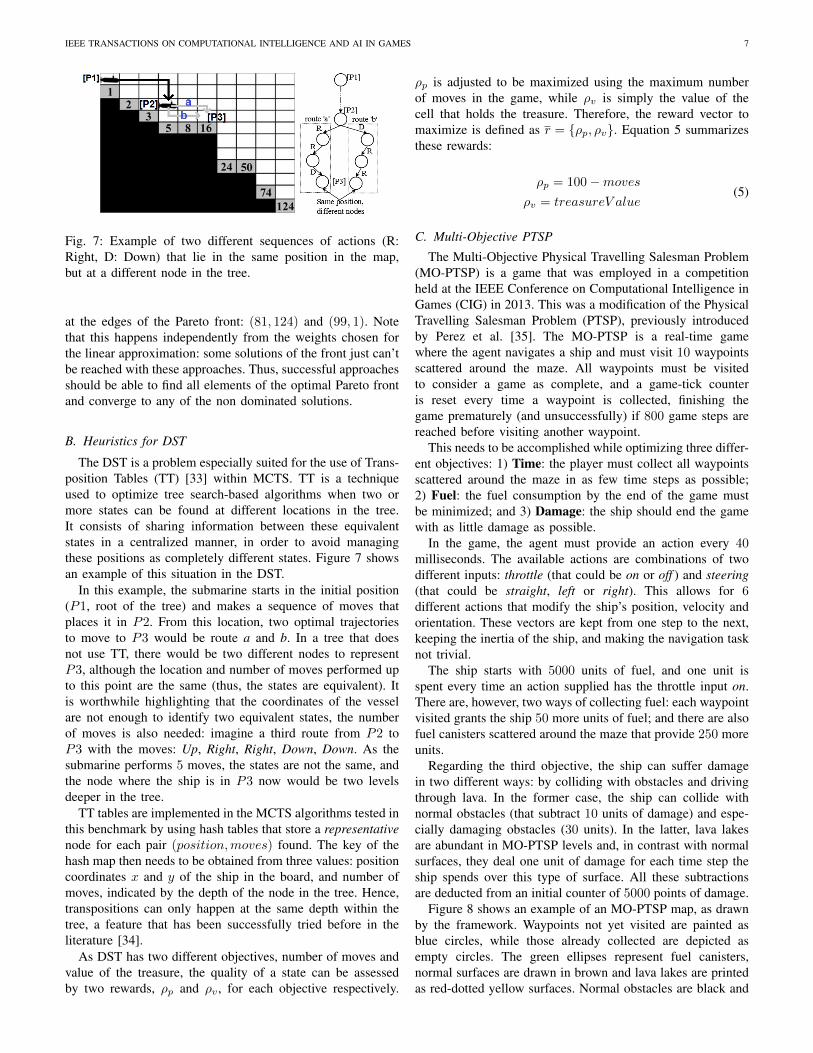
Fig. 7: Example of two different sequences of actions (R:Right, D: Down) that lie in the same position in the map,but at a different node in the tree.

at the edges of the Pareto front: (81, 124) and (99, 1). Notethat this happens independently from the weights chosen forthe linear approximation: some solutions of the front just can’tbe reached with these approaches. Thus, successful approachesshould be able to find all elements of the optimal Pareto frontand converge to any of the non dominated solutions.

B. Heuristics for DST

The DST is a problem especially suited for the use of Trans-position Tables (TT) [33] within MCTS. TT is a techniqueused to optimize tree search-based algorithms when two ormore states can be found at different locations in the tree.It consists of sharing information between these equivalentstates in a centralized manner, in order to avoid managingthese positions as completely different states. Figure 7 showsan example of this situation in the DST.

In this example, the submarine starts in the initial position(P1, root of the tree) and makes a sequence of moves thatplaces it in P2. From this location, two optimal trajectoriesto move to P3 would be route a and b. In a tree that doesnot use TT, there would be two different nodes to representP3, although the location and number of moves performed upto this point are the same (thus, the states are equivalent). Itis worthwhile highlighting that the coordinates of the vesselare not enough to identify two equivalent states, the numberof moves is also needed: imagine a third route from P2 toP3 with the moves: Up, Right, Right, Down, Down. As thesubmarine performs 5 moves, the states are not the same, andthe node where the ship is in P3 now would be two levelsdeeper in the tree.

TT tables are implemented in the MCTS algorithms tested inthis benchmark by using hash tables that store a representativenode for each pair (position,moves) found. The key of thehash map then needs to be obtained from three values: positioncoordinates x and y of the ship in the board, and number ofmoves, indicated by the depth of the node in the tree. Hence,transpositions can only happen at the same depth within thetree, a feature that has been successfully tried before in theliterature [34].

As DST has two different objectives, number of moves andvalue of the treasure, the quality of a state can be assessedby two rewards, ρp and ρv , for each objective respectively.

ρp is adjusted to be maximized using the maximum numberof moves in the game, while ρv is simply the value of thecell that holds the treasure. Therefore, the reward vector tomaximize is defined as r = ρp, ρv. Equation 5 summarizesthese rewards:

ρp = 100−movesρv = treasureV alue

(5)

C. Multi-Objective PTSP

The Multi-Objective Physical Travelling Salesman Problem(MO-PTSP) is a game that was employed in a competitionheld at the IEEE Conference on Computational Intelligence inGames (CIG) in 2013. This was a modification of the PhysicalTravelling Salesman Problem (PTSP), previously introducedby Perez et al. [35]. The MO-PTSP is a real-time gamewhere the agent navigates a ship and must visit 10 waypointsscattered around the maze. All waypoints must be visitedto consider a game as complete, and a game-tick counteris reset every time a waypoint is collected, finishing thegame prematurely (and unsuccessfully) if 800 game steps arereached before visiting another waypoint.

This needs to be accomplished while optimizing three differ-ent objectives: 1) Time: the player must collect all waypointsscattered around the maze in as few time steps as possible;2) Fuel: the fuel consumption by the end of the game mustbe minimized; and 3) Damage: the ship should end the gamewith as little damage as possible.

In the game, the agent must provide an action every 40milliseconds. The available actions are combinations of twodifferent inputs: throttle (that could be on or off ) and steering(that could be straight, left or right). This allows for 6different actions that modify the ship’s position, velocity andorientation. These vectors are kept from one step to the next,keeping the inertia of the ship, and making the navigation tasknot trivial.

The ship starts with 5000 units of fuel, and one unit isspent every time an action supplied has the throttle input on.There are, however, two ways of collecting fuel: each waypointvisited grants the ship 50 more units of fuel; and there are alsofuel canisters scattered around the maze that provide 250 moreunits.

Regarding the third objective, the ship can suffer damagein two different ways: by colliding with obstacles and drivingthrough lava. In the former case, the ship can collide withnormal obstacles (that subtract 10 units of damage) and espe-cially damaging obstacles (30 units). In the latter, lava lakesare abundant in MO-PTSP levels and, in contrast with normalsurfaces, they deal one unit of damage for each time step theship spends over this type of surface. All these subtractionsare deducted from an initial counter of 5000 points of damage.

Figure 8 shows an example of an MO-PTSP map, as drawnby the framework. Waypoints not yet visited are painted asblue circles, while those already collected are depicted asempty circles. The green ellipses represent fuel canisters,normal surfaces are drawn in brown and lava lakes are printedas red-dotted yellow surfaces. Normal obstacles are black and


Fig. 8: Sample MO-PTSP map.

damaging obstacles are drawn in red. Blue obstacles are elasticwalls that produce no damage to the ship. The vessel is drawnas a blue polygon and its trajectory is traced with a black line.

D. Heuristics for MO-PTSP

All the algorithms tested in the MO-PTSP in this researchemploy macro-actions, a concept that can be used for coars-ening the action space by applying the action chosen by thecontrol algorithm in several consecutive cycles, instead of justin the next one.

Previous research in PTSP [14], [36] suggests that usingmacro-actions for real-time navigation domains increases theperformance of the algorithms, and it has been used in theprevious PTSP competitions by the winner and other entries.

A macro-action of length L is defined as a repetition of agiven action during L consecutive time steps. The main ad-vantage of macro-actions is that the control algorithms can seefurther in the future, and then reduce the implication of open-endedness in real-time games (see Section II). As this reducesthe search space significantly, a better algorithm performanceis allowed. A consequence of using macro-actions is also thatthe algorithm can employ L consecutive steps to plan the nextmove (the next macro-action) to make. Therefore, instead ofspending 40 milliseconds, as in MO-PTSP, to define the nextaction, the algorithm can employ 40×L milliseconds for thistask, and hence perform a more extensive search.

In MO-PTSP, the macro-action size is L = 15, a valuethat has shown its proficiency before in PTSP. For moreinformation about macro-actions and their application to real-time navigation problems such as the PTSP, the reader isreferred to [14].

In order to evaluate a game state in MO-PTSP, threedifferent measures or rewards are taken, ρt, ρf , ρd, one foreach one of the objectives: time, fuel and damage, respectively.All these rewards are defined so they have to be maximized.The first reward uses a measure of distance for the timeobjective, as indicated in Equation 6:

ρt = 1− dt/dM (6)

The MO-PTSP framework includes a path-finding librarythat allows controllers to query the shortest distance of aroute of waypoints. dt indicates the distance from the currentposition until the last waypoint, following the desired route,and dM is the distance of the whole route from the startingposition. Minimizing the distance to the last waypoint willlead to the end of the game.

Equation 7 shows how the value of the fuel objective, ρf ,is obtained:

ρf = (1− (λt/λ0))× α+ ρt × (1− α) (7)

λt is the fuel consumed so far, and λ0 is the initial fuelat the start of the game. α is a value that balances betweenthe fuel component and the time objective from Equation 6.Note that, as waypoints need to keep being visited, it isnecessary to include a distance measure for this reward.Otherwise, an approach that prioritizes this objective wouldnot minimize distance to waypoints at all (the ship could juststand still: no fuel consumed is optimal), and therefore wouldnot complete the game. The value of α has been determinedempirically, in order to provide a good balance between thesetwo components, and is set to 0.66.

Finally, Equation 8 gives the method used to calculate thedamage objective, ρd:

ρd =

(1− (gt/gM ))× β1 + ρt × (1− β1), sp > γ

(1− (gt/gM ))× β2 + ρt × (1− β2), sp ≤ γ(8)

gt is the damage suffered so far in the game, and gM isthe maximum damage the ship can take. In this case, threedifferent variables are used to regulate the behaviour of thisobjective: γ, β1 and β2. Both β1 and β2 have the same roleas α in Equation 7: they balance between the time objectiveand the damage measure. The difference is that β1 is used inhigh speeds, while β2 is employed with low velocities. Thisis distinguished by the parameter γ, that can be seen as athreshold value for the ship’s speed (sp). This differentiationis made in order to avoid low speeds in lava lakes, as thissignificantly increases the damage suffered. The values forthese variables have also been determined empirically, andthey are set to γ = 0.8, β1 = 0.75 and β2 = 0.25.

The final reward vector to be maximized is thereforer = ρt, ρf , ρd. It is important to highlight again that thesethree rewards are the same for all the algorithms tested in theexperiments.

VI. EXPERIMENTATION

The experiments performed in this research compare threedifferent algorithms in the two benchmarks presented in Sec-tion V: a single objective MCTS (referred to here simplyas MCTS), the Multi-Objective MCTS (MO-MCTS) and arolling horizon version of the NSGA-II algorithm describedin Section III (NSGA-II). This NSGA-II version evolves apopulation where the individuals are sequences of actions(macro-actions in the MO-PTSP case), obtaining the fitnessfrom the state of the game after applying the sequence. Thepopulation sizes, determined empirically, were set to 20 and


50 individuals for DST and MO-PTSP respectively. The valueof C in Equation 1 and 4 is set to

√2.

All the algorithms have a limited number of evaluationsbefore providing an action to perform. In order for thesegames to be real-time, the time budget allowed is close to 40milliseconds. With the objective of avoiding congestion peaksat the machine where the experiments are run, the averagenumber of evaluations possible in 40 ms is calculated andemployed in the tests. This leads to 4500 evaluations in theDST, and 500 evaluations for MO-PTSP, using the same serverwhere the PTSP and MO-PTSP competitions were run2.

A. Results in DST

As the optimal Pareto front of the DST is known, a measureof performance can be obtained by observing the percentage oftimes these solutions are found by the players. As the solutionthat the algorithms converge to depends on the weights vectoremployed during the search (see end of Section IV), theapproach taken here is to provide different weight vectors Wand analyze them separately.

The weight vector for DST has two dimensions. This vectoris here referred to as W = (wp, wv), where wp weights moves;and wv weights the treasure value (wv = 1 − wp). wp takesvalues between 0 and 1, with a precision of 0.01, and 100 runshave been performed for each pair (wp, wv). Hence, the gamehas been played a total of 10000 times, for each algorithm.

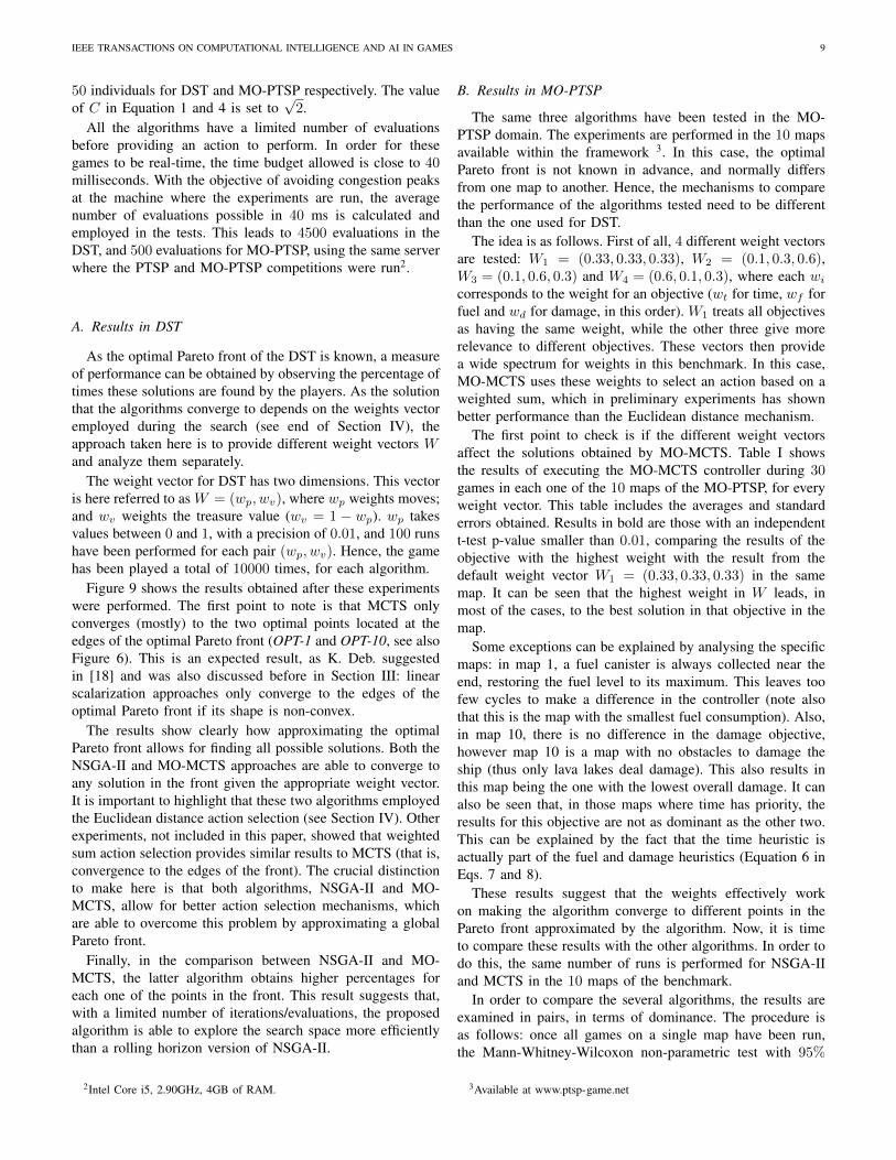
Figure 9 shows the results obtained after these experimentswere performed. The first point to note is that MCTS onlyconverges (mostly) to the two optimal points located at theedges of the optimal Pareto front (OPT-1 and OPT-10, see alsoFigure 6). This is an expected result, as K. Deb. suggestedin [18] and was also discussed before in Section III: linearscalarization approaches only converge to the edges of theoptimal Pareto front if its shape is non-convex.

The results show clearly how approximating the optimalPareto front allows for finding all possible solutions. Both theNSGA-II and MO-MCTS approaches are able to converge toany solution in the front given the appropriate weight vector.It is important to highlight that these two algorithms employedthe Euclidean distance action selection (see Section IV). Otherexperiments, not included in this paper, showed that weightedsum action selection provides similar results to MCTS (that is,convergence to the edges of the front). The crucial distinctionto make here is that both algorithms, NSGA-II and MO-MCTS, allow for better action selection mechanisms, whichare able to overcome this problem by approximating a globalPareto front.

Finally, in the comparison between NSGA-II and MO-MCTS, the latter algorithm obtains higher percentages foreach one of the points in the front. This result suggests that,with a limited number of iterations/evaluations, the proposedalgorithm is able to explore the search space more efficientlythan a rolling horizon version of NSGA-II.

2Intel Core i5, 2.90GHz, 4GB of RAM.

B. Results in MO-PTSP

The same three algorithms have been tested in the MO-PTSP domain. The experiments are performed in the 10 mapsavailable within the framework 3. In this case, the optimalPareto front is not known in advance, and normally differsfrom one map to another. Hence, the mechanisms to comparethe performance of the algorithms tested need to be differentthan the one used for DST.

The idea is as follows. First of all, 4 different weight vectorsare tested: W1 = (0.33, 0.33, 0.33), W2 = (0.1, 0.3, 0.6),W3 = (0.1, 0.6, 0.3) and W4 = (0.6, 0.1, 0.3), where each wi

corresponds to the weight for an objective (wt for time, wf forfuel and wd for damage, in this order). W1 treats all objectivesas having the same weight, while the other three give morerelevance to different objectives. These vectors then providea wide spectrum for weights in this benchmark. In this case,MO-MCTS uses these weights to select an action based on aweighted sum, which in preliminary experiments has shownbetter performance than the Euclidean distance mechanism.

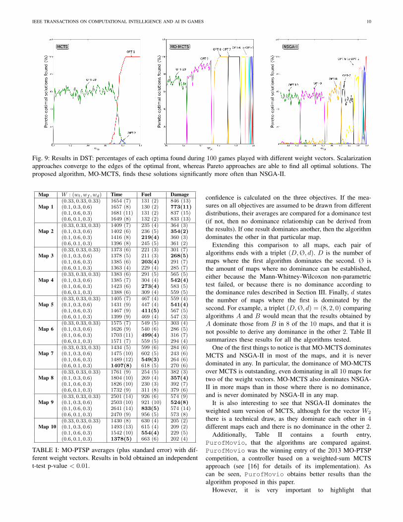
The first point to check is if the different weight vectorsaffect the solutions obtained by MO-MCTS. Table I showsthe results of executing the MO-MCTS controller during 30games in each one of the 10 maps of the MO-PTSP, for everyweight vector. This table includes the averages and standarderrors obtained. Results in bold are those with an independentt-test p-value smaller than 0.01, comparing the results of theobjective with the highest weight with the result from thedefault weight vector W1 = (0.33, 0.33, 0.33) in the samemap. It can be seen that the highest weight in W leads, inmost of the cases, to the best solution in that objective in themap.

Some exceptions can be explained by analysing the specificmaps: in map 1, a fuel canister is always collected near theend, restoring the fuel level to its maximum. This leaves toofew cycles to make a difference in the controller (note alsothat this is the map with the smallest fuel consumption). Also,in map 10, there is no difference in the damage objective,however map 10 is a map with no obstacles to damage theship (thus only lava lakes deal damage). This also results inthis map being the one with the lowest overall damage. It canalso be seen that, in those maps where time has priority, theresults for this objective are not as dominant as the other two.This can be explained by the fact that the time heuristic isactually part of the fuel and damage heuristics (Equation 6 inEqs. 7 and 8).

These results suggest that the weights effectively workon making the algorithm converge to different points in thePareto front approximated by the algorithm. Now, it is timeto compare these results with the other algorithms. In order todo this, the same number of runs is performed for NSGA-IIand MCTS in the 10 maps of the benchmark.

In order to compare the several algorithms, the results areexamined in pairs, in terms of dominance. The procedure isas follows: once all games on a single map have been run,the Mann-Whitney-Wilcoxon non-parametric test with 95%

3Available at www.ptsp-game.net

www.ptsp-game.net


Fig. 9: Results in DST: percentages of each optima found during 100 games played with different weight vectors. Scalarizationapproaches converge to the edges of the optimal front, whereas Pareto approaches are able to find all optimal solutions. Theproposed algorithm, MO-MCTS, finds these solutions significantly more often than NSGA-II.

Map W : (wt, wf , wd) Time Fuel Damage

Map 1(0.33, 0.33, 0.33) 1654 (7) 131 (2) 846 (13)(0.1, 0.3, 0.6) 1657 (8) 130 (2) 773(11)(0.1, 0.6, 0.3) 1681 (11) 131 (2) 837 (15)(0.6, 0.1, 0.3) 1649 (8) 132 (2) 833 (13)

Map 2(0.33, 0.33, 0.33) 1409 (7) 235 (4) 364 (3)(0.1, 0.3, 0.6) 1402 (6) 236 (5) 354(2)(0.1, 0.6, 0.3) 1416 (8) 219(4) 360 (3)(0.6, 0.1, 0.3) 1396 (8) 245 (5) 361 (2)

Map 3(0.33, 0.33, 0.33) 1373 (6) 221 (3) 301 (7)(0.1, 0.3, 0.6) 1378 (5) 211 (3) 268(5)(0.1, 0.6, 0.3) 1385 (6) 203(4) 291 (7)(0.6, 0.1, 0.3) 1363 (4) 229 (4) 285 (7)

Map 4(0.33, 0.33, 0.33) 1383 (6) 291 (5) 565 (5)(0.1, 0.3, 0.6) 1385 (7) 304 (4) 542(4)(0.1, 0.6, 0.3) 1423 (6) 273(4) 583 (5)(0.6, 0.1, 0.3) 1388 (6) 309 (4) 559 (5)

Map 5(0.33, 0.33, 0.33) 1405 (7) 467 (4) 559 (4)(0.1, 0.3, 0.6) 1431 (9) 447 (4) 541(4)(0.1, 0.6, 0.3) 1467 (9) 411(5) 567 (5)(0.6, 0.1, 0.3) 1399 (9) 469 (4) 547 (3)

Map 6(0.33, 0.33, 0.33) 1575 (7) 549 (5) 303 (4)(0.1, 0.3, 0.6) 1626 (9) 540 (6) 286 (5)(0.1, 0.6, 0.3) 1703 (11) 499(4) 316 (7)(0.6, 0.1, 0.3) 1571 (7) 559 (5) 294 (4)

Map 7(0.33, 0.33, 0.33) 1434 (5) 599 (6) 284 (6)(0.1, 0.3, 0.6) 1475 (10) 602 (5) 243 (6)(0.1, 0.6, 0.3) 1489 (12) 549(3) 264 (6)(0.6, 0.1, 0.3) 1407(8) 618 (5) 270 (6)

Map 8(0.33, 0.33, 0.33) 1761 (9) 254 (5) 382 (3)(0.1, 0.3, 0.6) 1804 (10) 269 (4) 357(4)(0.1, 0.6, 0.3) 1826 (10) 230 (3) 392 (7)(0.6, 0.1, 0.3) 1732 (9) 311 (8) 379 (6)

Map 9(0.33, 0.33, 0.33) 2501 (14) 926 (6) 574 (9)(0.1, 0.3, 0.6) 2503 (10) 921 (10) 524(8)(0.1, 0.6, 0.3) 2641 (14) 833(5) 574 (14)(0.6, 0.1, 0.3) 2470 (9) 956 (5) 573 (8)

Map 10(0.33, 0.33, 0.33) 1430 (8) 630 (4) 205 (2)(0.1, 0.3, 0.6) 1493 (13) 615 (4) 209 (2)(0.1, 0.6, 0.3) 1542 (10) 554(4) 229 (5)(0.6, 0.1, 0.3) 1378(5) 663 (6) 202 (4)

TABLE I: MO-PTSP averages (plus standard error) with dif-ferent weight vectors. Results in bold obtained an independentt-test p-value < 0.01.

confidence is calculated on the three objectives. If the mea-sures on all objectives are assumed to be drawn from differentdistributions, their averages are compared for a dominance test(if not, then no dominance relationship can be derived fromthe results). If one result dominates another, then the algorithmdominates the other in that particular map.

Extending this comparison to all maps, each pair ofalgorithms ends with a triplet (D,Ø, d). D is the number ofmaps where the first algorithm dominates the second. Ø isthe amount of maps where no dominance can be established,either because the Mann-Whitney-Wilcoxon non-parametrictest failed, or because there is no dominance according tothe dominance rules described in Section III. Finally, d statesthe number of maps where the first is dominated by thesecond. For example, a triplet (D,Ø, d) = (8, 2, 0) comparingalgorithms A and B would mean that the results obtained byA dominate those from B in 8 of the 10 maps, and that it isnot possible to derive any dominance in the other 2. Table IIsummarizes these results for all the algorithms tested.

One of the first things to notice is that MO-MCTS dominatesMCTS and NSGA-II in most of the maps, and it is neverdominated in any. In particular, the dominance of MO-MCTSover MCTS is outstanding, even dominating in all 10 maps fortwo of the weight vectors. MO-MCTS also dominates NSGA-II in more maps than in those where there is no dominance,and is never dominated by NSGA-II in any map.

It is also interesting to see that NSGA-II dominates theweighted sum version of MCTS, although for the vector W2

there is a technical draw, as they dominate each other in 4different maps each and there is no dominance in the other 2.

Additionally, Table II contains a fourth entry,PurofMovio, that the algorithms are compared against.PurofMovio was the winning entry of the 2013 MO-PTSPcompetition, a controller based on a weighted-sum MCTSapproach (see [16] for details of its implementation). Ascan be seen, PurofMovio obtains better results than thealgorithm proposed in this paper.

However, it is very important to highlight that


W : (wt, wf , wd) MO-MCTS (D,Ø, d) MCTS (D,Ø, d) NSGA-II (D,Ø, d) PurofMovio (D,Ø, d)

MO-MCTSW1 : (0.33, 0.33, 0.33)

−(8, 2, 0) (8, 2, 0) (0, 5, 5)

W2 : (0.1, 0.3, 0.6) (10, 0, 0) (4, 6, 0) (0, 6, 4)W3 : (0.1, 0.6, 0.3) (8, 2, 0) (7, 3, 0) (0, 5, 5)W4 : (0.6, 0.1, 0.3) (10, 0, 0) (3, 7, 0) (0, 3, 7)

MCTSW1 : (0.33, 0.33, 0.33) (0, 8, 2)

−(0, 2, 8) (0, 2, 8)

W2 : (0.1, 0.3, 0.6) (0, 0, 10) (4, 2, 4) (0, 3, 7)W3 : (0.1, 0.6, 0.3) (0, 2, 8) (0, 1, 9) (0, 6, 4)W4 : (0.6, 0.1, 0.3) (0, 0, 10) (3, 3, 4) (0, 1, 9)

NSGA-IIW1 : (0.33, 0.33, 0.33) (0, 2, 8) (8, 2, 0)

−(0, 4, 6)

W2 : (0.1, 0.3, 0.6) (0, 6, 4) (4, 2, 4) (0, 4, 6)W3 : (0.1, 0.6, 0.3) (0, 3, 7) (9, 1, 0) (0, 5, 5)W4 : (0.6, 0.1, 0.3) (0, 7, 3) (4, 3, 3) (0, 4, 6)

PurofMovioW1 : (0.33, 0.33, 0.33) (5, 5, 0) (8, 2, 0) (6, 4, 0)

−W2 : (0.1, 0.6, 0.3) (4, 6, 0) (7, 3, 0) (6, 4, 0)W3 : (0.1, 0.3, 0.6) (5, 5, 0) (6, 4, 0) (5, 5, 0)W4 : (0.6, 0.1, 0.3) (7, 3, 0) (9, 1, 0) (6, 4, 0)

TABLE II: Results in MO-PTSP: Each cell indicates the triplet (D,Ø, d), where D is the number of maps where the rowalgorithm dominates the column one, Ø is the amount of maps where no dominance can be established, and d states thenumber of maps where the row algorithm is dominated by the column one. All the algorithms followed the same route (orderof waypoints and fuel canisters) in every map tested.

PurofMovio is not using the same heuristics as theones presented in this research. Hence, nothing can beconcluded from making pairwise comparisons directly withthe winning entry of the competition. It is likely thatPurofMovio’s heuristics are more efficient than the onespresented here, but the goal of this paper is not to developthe best heuristics for the MO-PTSP, but to provide an insightinto how a multi-objective version of MCTS compares toother algorithms using the same heuristics.

Nonetheless, the inclusion of PurofMovio in this compar-ison is not pointless: it is possible to assess the quality of thethree algorithms tested here by comparing their performancerelatively, against this high quality entry. Attending to thiscriteria, it can be seen how MO-MCTS is the algorithm thatis dominated less often by PurofMovio, producing similarresults on an average of 4.75 out of the 10 maps, and beingdominated in 5.25 maps. MCTS and NSGA-II are dominatedmore often than MO-MCTS, being dominated in an averageof 7.5 and 5.75 of the maps, respectively. This comparativeresult shows again that MO-MCTS is achieving the best resultsamong the three algorithms compared here.

C. A step further in MO-PTSP: segments and weights

There is another aspect that can be further improved inthe MO-PTSP benchmark, and is also applicable to otherdomains. It is naive to think that a unique weight vector willbe the ideal one for the whole game. Specifically in the MO-PTSP, there are regions of the map where there are moreobstacles or lava lakes, hence the ship is most likely to sufferhigher damage there. Also, the route followed during the gameaffects the relative ideal speed between waypoints, or perhapsa fuel canister may be picked up, which will affect how thefuel objective will be managed. In general, many real-timegames go through different phases, with different objectivesand priorities.

A way to provide different weights at different times in MO-PTSP is straightforward. Given the route of waypoints (andfuel canisters) being followed, one can divide it into segments,

where each segment starts and ends with a waypoint (or fuelcanister). Then, each segment can be assigned a particularweight vector W .

The question is then how to assign these weight vectors.Three different ways can be devised:• Manually set the weight vectors. This was attempted and

it proved to be a non trivial task.• Setting the appropriate weight for each segment dy-

namically, based on the segment’s characteristics. Thisinvolves the creation or discovery of features and somekind of function approximation to assign the values.

• Learn, for each specific map, the combination of weightvectors that produces better results.

This section shows some initial results obtained when test-ing the third variant, using a stochastic hill climbing algorithmon each map. The goal is to check if, by varying the weightvectors between segments, better solutions can be achieved.

An individual is identified by a string of integers, whereeach integer refers to one of the weight vectors utilizedin the previous sections ( 1 = W1 = (0.33, 0.33, 0.33),2 = W2 = (0.1, 0.3, 0.6) and 3 = W3 = (0.1, 0.6, 0.3). W4

has been left out of this experiment, as it has shown to bethe least influential weight vector). The solution is evaluatedplaying a particular map 10 times, and its fitness is obtainedby calculating the average of those runs. A population of 10individuals is kept, and the solutions of the initial populationare created either randomly, or mutated from base individuals.These base individuals all have segments with the same weightvector W1, W2, or W3.

The best solution, determined by dominance, is kept andpromoted to the next generation, where it is mutated togenerate other individuals of the population. Also, a portionof the individuals of the next population is created uniformlyat random at every generation, until the end of the algorithm,which is established at 50 generations.

Table III shows the results obtained on each run, one permap. Each row corresponds to a run in the associated map, andit provides different results depending on the weights vector.


Map Weight genome Time Fuel Damage D

Map 111111111111111 1654 (7) 131 (2) 846 (13) 22222222222222 1657 (8) 130 (2) 773 (11) 33333333333333 1681 (11) 131 (2) 837 (15) 32312212331112 1619 (12) 130 (2) 744 (15)

Map 211111111111111 1409 (7) 235 (4) 364 (3) 22222222222222 1402 (6) 236 (5) 354 (2) 33333333333333 1416 (8) 219 (4) 360 (3) 23131312323213 1390 (10) 210 (3) 353 (3)

Map 311111111111111 1373 (6) 221 (3) 301 (7) 22222222222222 1378 (5) 211 (3) 268 (5) 33333333333333 1385 (6) 203 (4) 291 (7) Ø11122222112231 1358 (9) 219 (7) 263 (12)

Map 411111111111111 1383 (6) 291 (5) 565 (5) 22222222222222 1385 (7) 304 (4) 542 (4) 33333333333333 1423 (6) 273 (4) 583 (5) Ø11121131212112 1360 (4) 282 (5) 540 (4)

Map 511111111111111 1405 (7) 467 (4) 559 (4) 22222222222222 1431 (9) 447 (4) 541 (4) 33333333333333 1467 (9) 411 (5) 567 (5) Ø21311213111211 1397 (11) 448 (10) 535 (5)

Map 611111111111111 1575 (7) 549 (5) 303 (4) 22222222222222 1626 (9) 540 (6) 286 (5) 33333333333333 1703 (11) 499 (4) 316 (7) Ø31121312111111 1570 (16) 535 (10) 266 (6)

Map 711111111111111 1434 (5) 599 (6) 284 (6) 22222222222222 1475 (10) 602 (5) 243 (6) 33333333333333 1489 (12) 549 (3) 264 (6) Ø11332211321332 1401 (12) 563 (4) 230 (12)

Map 811111111111111 1761 (9) 254 (5) 382 (3) 22222222222222 1804 (10) 269 (4) 357 (4) 33333333333333 1826 (10) 230 (3) 392 (7) Ø23221131313323 1747 (11) 247 (9) 363 (9)

Map 911111111111111 2501 (14) 926 (6) 574 (9) 22222222222222 2503 (10) 921 (10) 524 (8) 33333333333333 2641 (14) 833 (5) 574 (14) Ø21132331333223 2463 (19) 891 (8) 523 (9)

Map 1011111111111111 1430 (8) 630 (4) 205 (2) 22222222222222 1493 (13) 615 (4) 209 (2) 33333333333333 1542 (10) 554 (4) 229 (5) Ø11311111322231 1418 (9) 623 (9) 197 (2)

TABLE III: MO-PTSP Results with different weights. The lastcolumn indicates if the evolved individual dominates () ornot (Ø) each one of the base genomes for that particular map.

The top three are the base individuals, taken from Table IIfor comparison. The forth result on each row is the best oneafter the run. Each genome is a string of the form abc . . . z,that represents WaWbWc . . .Wz , where each element is aweight vector used in that particular segment. The last columnindicates if the evolved individual dominates () or not (Ø)each one of the base genomes for that particular map.

The results suggest some interesting ideas. First of all,it is indeed possible to obtain better results by varying theweights of the objectives along the route: in 22 out of the30 comparisons made, the evolved solution dominates thebase individuals and, in the other 8, both solutions in thecomparison would be in the same Pareto front of solutions.

If the focus is set on what particular weights are moresuccessful, it is interesting to see that the best configurationsfound are better, in all maps, than the base individuals with allweights equal to W1 (wt = 0.33, wf = 0.33, wd = 0.33) andW2 (wt = 0.1, wf = 0.3, wd = 0.6). In other words, it wasalways possible to find a combination of weight vectors thatperformed better than approaches that gave the same weight

to all objectives, and also better than the ones that prioritizelow damage.

It is also worthwhile mentioning that in those cases wheredominance over the base individual was not achieved, the basewas the one that prioritized fuel. Actually, it can be seen thatin these cases, the result in the fuel objective is the one thatprevents the dominance from happening, obtaining a bettervalue than the evolved solution in this particular objective.

VII. CONCLUSIONS AND FUTURE WORK

This paper presents a multi-objective version of MonteCarlo Tree Search (MO-MCTS) for real-time games: scenarioswhere the time budget allowed for finding out the best possibleaction to apply next is close to 40ms. MO-MCTS is tested,in comparison with a single-objective MCTS algorithm anda rolling horizon NSGA-II, in two different real-time games,the Deep Sea Treasure (DST) and the Multi-Objective PhysicalTravelling Salesman Problem (MO-PTSP). This comparison ismade by using the same heuristics that determine the value ofa given state, so the focus is set on how the algorithms explorethe search space on each problem.

The results obtained in this study show the strength of thealgorithm proposed, as it provides better solutions than theones obtained by the other algorithms in comparison. Also, theMO-MCTS approach samples successfully across the differentsolutions in the Pareto front (optimal front in the DST, thebest found in MO-PTSP), depending on the weights providedfor each objective. Finally, some initial results are obtainedapplying the idea of using distinct weight vectors for theobjectives in different situations within the game, showing thatit is possible to improve the performance of the algorithms.

The stochastic hill climbing algorithm used for creatingstrings of weight vectors for the MO-PTSP is relatively simple,although it was able to obtain very good results in fewiterations. However, it could be desirable to model behavioursthat dynamically change the weight vectors according tomeasurements of the game state, instead of evolving a differentsolution for each particular map. A possible extension for thiswork is to analyse and discover features in the game statethat allows the establishment of relationships between gamesituations and the weight vectors to use for each objective.This mechanism would be general enough to be applicable tomany different maps without requiring specific learning in anyparticular level.

Finally, the results described in this paper allow us toassume that multi-objective approaches can provide a highquality level of play in real-time games. Multi-objective prob-lems pop up in different settings and by using MCTS wecan balance not only between exploration and exploitation butbetween multiple objectives as well.

ACKNOWLEDGMENTS

This work was supported by EPSRC grants EP/H048588/1,under the project entitled “UCT for Games and Beyond”. Theauthors would also like to thank Edward Powley and DanielWhitehouse for their work in the controller PurofMovio forthe MO-PTSP competition.


REFERENCES

[1] R. T. Marler and J. S. Arora, “Survey of Multi-objective OptimizationMethods for Engineering,” Structural and Multidisciplinary Optimiza-tion, vol. 26, pp. 369–395, 2004.

[2] C. Coello, Handbook of Research on Nature Inspired Computing forEconomy and Management. Idea Group Publishing, 2006, ch. Evolu-tionary Multi-Objective Optimization and its Use in Finance.

[3] D. Perez, S. Samothrakis, and S. Lucas, “Online and Offline Learningin Multi-Objective Monte Carlo Tree Search,” in Proceedings of theConference on Computational Intelligence and Games (CIG), 2013, pp.121–128.

[4] C.-S. Lee, M.-H. Wang, G. M. J.-B. Chaslot, J.-B. Hoock, A. Rimmel,O. Teytaud, S.-R. Tsai, S.-C. Hsu, and T.-P. Hong, “The ComputationalIntelligence of MoGo Revealed in Taiwan’s Computer Go Tournaments,”IEEE Transactions on Computational Intelligence and AI in Games,vol. 1, no. 1, pp. 73–89, 2009.

[5] C. Browne, E. Powley, D. Whitehouse, S. Lucas, P. Cowling, P. Rohlf-shagen, S. Tavener, D. Perez, S. Samothrakis, and S. Colton, “ASurvey of Monte Carlo Tree Search Methods,” IEEE Transactions onComputational Intelligence and AI in Games, vol. 4:1, pp. 1–43, 2012.

[6] G. M. J.-B. Chaslot, M. H. M. Winands, H. J. van den Herik,J. W. H. M. Uiterwijk, and B. Bouzy, “Progressive Strategies forMonte-Carlo Tree Search,” New Math. Nat. Comput., vol. 4, no. 3,pp. 343–357, 2007. [Online]. Available: http://citeseerx.ist.psu.edu/viewdoc/download?doi=10.1.1.77.9239&rep=rep1&type=pdf

[7] L. Kocsis and C. Szepesvari, “Bandit based Monte-Carlo planning,”Machine Learning: ECML 2006, vol. 4212, pp. 282–293, 2006.

[8] P.-A. Coquelin, R. Munos et al., “Bandit Algorithms for Tree Search,”in Uncertainty in Artificial Intelligence, 2007.

[9] D. Robles and S. M. Lucas, “A Simple Tree Search Method for PlayingMs. Pac-Man,” in Proceedings of the IEEE Conference of ComputationalIntelligence in Games, Milan, Italy, 2009, pp. 249–255.

[10] S. Samothrakis, D. Robles, and S. M. Lucas, “Fast Approximate Max-n Monte-Carlo Tree Search for Ms Pac-Man,” IEEE Transactions onComputational Intelligence and AI in Games, vol. 3, no. 2, pp. 142–154, 2011.

[11] N. Ikehata and T. Ito, “Monte Carlo Tree Search in Ms. Pac-Man,” inProc. 15th Game Progrramming Workshop, Kanagawa, Japan, 2010, pp.1–8.

[12] M. P. D. Schadd, M. H. M. Winands, H. J. van den Herik, G. M. J.-B.Chaslot, and J. W. H. M. Uiterwijk, “Single-Player Monte-Carlo TreeSearch,” in Proceedings of Computer Games, LNCS 5131, 2008, pp.1–12.

[13] T. Cazenave, “Reflexive Monte-Carlo Search,” in Proc. Comput. GamesWorkshop, Amsterdam, Netherlands, 2007, pp. 165–173.

[14] D. Perez, E. J. Powley, D. Whitehouse, P. Rohlfshagen, S. Samothrakis,P. I. Cowling, and S. M. Lucas, “Solving the Physical Travelling Sales-man Problem: Tree Search and Macro-Actions,” IEEE Trans. Comp.Intell. AI Games, pp. 1–16, 2013.

[15] E. J. Powley, D. Whitehouse, and P. I. Cowling, “Monte Carlo TreeSearch with Macro-Actions and Heuristic Route Planning for the Phys-ical Travelling Salesman Problem,” in Proc. IEEE Conf. Comput. Intell.Games, 2012, pp. 234–241.

[16] ——, “Monte Carlo Tree Search with Macro-Actions and HeuristicRoute Planning for the Multiobjective Physical Travelling SalesmanProblem,” in Proc. IEEE Conf. Comput. Intell. Games, 2013, pp. 73–80.

[17] D. Brockhoff, “Tutorial on evolutionary multiobjective optimization,” inProceedings of the 15th Annual Conference Companion on Genetic andEvolutionary Computation, 2013, pp. 307–334.

[18] K. Deb, Multi-Objective Optimization using Evolutionary Algorithms.Wiley, 2001.

[19] C. Coello, “An Updated Survey of Evolutionary Multiobjective Opti-mization Techniques: State of the Art and Future Trends,” in Proc. ofthe Congress on Evolutionary Computation, 1999, pp. 3–13.

[20] A. Zhou, B.-Y. Qu, H. Li, S.-Z. Zhao, P. N. Suganthan, and Q. Zhang,“Multiobjective Evolutionary Algorithms: A Survey of the State of theArt,” Swarm and Evolutionary Computation, vol. 1, pp. 32–49, 2011.

[21] K. Deb, A. Pratap, S. Agarwal, and T. Meyarivan, “A Fast ElitistMulti-Objective Genetic Algorithm: NSGA-II,” IEEE Transactions onEvolutionary Computation, vol. 6, pp. 182–197, 2002.

[22] H. Jain and K. Deb, “An Improved Adaptive Approach for ElitistNondominated Sorting Genetic Algorithm for Many-Objective Opti-mization,” in Evolutionary Multi-Criterion Optimization, ser. LectureNotes in Computer Science, R. Purshouse, P. Fleming, C. Fonseca,S. Greco, and J. Shaw, Eds. Springer Berlin Heidelberg, 2013, vol.7811, pp. 307–321.

[23] N. Beume, B. Naujoks, and M. Emmerich, “SMS-EMOA: MultiobjectiveSelection Based on Dominated Hypervolume,” European Journal ofOperational Research, vol. 181, no. 3, pp. 1653–1669, 2007.

[24] Q. Zhang and H. Li, “MOEA/D: A Multiobjective Evolutionary Algo-rithm Based on Decomposition,” IEEE Transactions on EvolutionaryComputation, vol. 11, no. 6, pp. 712–731, 2007.

[25] R. Sutton and A. Barto, Reinforcement Learning: An Introduction(Adaptive Computation and Machine Learning). A Bradford Book,1998.

[26] P. Vamplew, R. Dazeley, A. Berry, R. Issabekov, and E. Dekker, “Em-pirical Evaluation Methods for Multiobjective Reinforcement LearningAlgorithms,” Machine Learning, vol. 84, pp. 51–80, 2010.

[27] Z. Gabor, Z. Kalmar, and C. Szepesvari, “Multi-criteria ReinforcementLearning,” in The fifteenth international conference on machine learning,1998, pp. 197–205.

[28] S. Natarajan and P. Tadepalli, “Dynamic Preferences in Multi-CriteriaReinforcement Learning,” in In Proceedings of International Conferenceof Machine Learning, 2005, pp. 601–608.

[29] L. Barrett and S. Narayanan, “Learning All Optimal Policies withMultiple Criteria,” in Proceedings of the international conference onmachine learning, 2008, pp. 41–47.

[30] E. Zitzler, Evolutionary Algorithms for Multiobjective Optimization:Methods and Applications. TIK-Schriftenreihe Nr. 30, Diss ETH No.13398, Swiss Federal Institute of Technology (ETH) Zurich: ShakerVerlag, Germany, 1999.

[31] W. Weijia and M. Sebag, “Multi-objective Monte Carlo Tree Search,” inProceedings of the Asian Conference on Machine Learning, 2012, pp.507–522.

[32] ——, “Hypervolume indicator and dominance reward based multi-objective Monte-Carlo Tree Search,” Machine Learning, vol. 92:2–3,pp. 403–429, 2013.

[33] B. E. Childs, J. H. Brodeur, and L. Kocsis, “Transpositions and MoveGroups in Monte Carlo Tree Search,” in Proceedings of IEEE Sympo-sium on Computational Intelligence and Games, 2008, pp. 389–395.

[34] T. Kozelek, “Methods of MCTS and the game Arimaa,” M.S. thesis,Charles Univ., Prague, 2009.

[35] D. Perez, P. Rohlfshagen, and S. Lucas, “The Physical TravellingSalesman Problem: WCCI 2012 Competition,” in Proceedings of theIEEE Congress on Evolutionary Computation, 2012, pp. 1–8.

[36] ——, “Monte Carlo Tree Search: Long Term versus Short TermPlanning,” in Proceedings of the IEEE Conference on ComputationalIntelligence and Games, 2012, pp. 219 – 226.

Diego Perez is currently pursuing a Ph.D. in Artifi-cial Intelligence applied to games at the Universityof Essex (UK). He has published in the domain ofGame AI, with research interests on ReinforcementLearning and Evolutionary Computation. He hasorganized several Game AI competitions, as thePhysical Travelling Salesman Problem and the Gen-eral Video Game AI competitions, both held in IEEEconferences. He also has programming experiencein the videogames industry with titles published forgame consoles and PC.

Sanaz Mostaghim is a professor of computer sci-ence at the Otto von Guericke University Magde-burg, Germany. Her current research interests are inthe field of evolutionary computation, particularlyin the areas of evolutionary multi-objective opti-mization, swarm intelligence and their applicationsin science and industry. She is an active IEEEmember and is serving as an associate editor forIEEE Transactions on Evolutionary Computationand IEEE Transactions on Cybernetics.

http://citeseerx.ist.psu.edu/viewdoc/download?doi=10.1.1.77.9239&rep=rep1&type=pdf

http://citeseerx.ist.psu.edu/viewdoc/download?doi=10.1.1.77.9239&rep=rep1&type=pdf


Spyridon Samothrakis is currently a Senior Re-search Officer at the University of Essex. He holdsa B.Sc. from the University of Sheffield (ComputerScience), an M.Sc. from the University of Sussex(Intelligent Systems) and a Ph.D (Computer Sci-ence) from the University of Essex. His interestsinclude game theory, machine learning, evolutionaryalgorithms and consciousness.

Simon Lucas (SMIEEE) is a professor of ComputerScience at the University of Essex (UK) wherehe leads the Game Intelligence Group. His mainresearch interests are games, evolutionary compu-tation, and machine learning, and he has publishedwidely in these fields with over 160 peer-reviewedpapers. He is the inventor of the scanning n-tupleclassifier, and is the founding Editor-in-Chief of theIEEE Transactions on Computational Intelligenceand AI in Games.

Multi-Objective Monte Carlo Tree Search for Real-Time...

Documents

Transcript of Multi-Objective Monte Carlo Tree Search for Real-Time...