Proceedings of the 2020 Winter Simulation ConferenceK.-H. Bae, B. Feng, S. Kim, S. Lazarova-Molnar, Z. Zheng, T. Roeder, and R. Thiesing, eds.

A TUTORIAL INTRODUCTION TO MONTE CARLO TREE SEARCH

Michael C. Fu

Robert H. Smith School of Business, Van Munching HallInstitute for Systems Research, A. V. Williams Building

University of MarylandCollege Park, MD 20742, USA

ABSTRACT

This tutorial provides an introduction to Monte Carlo tree search (MCTS), which is a general approach tosolving sequential decision-making problems under uncertainty using stochastic (Monte Carlo) simulation.MCTS is most famous for its role in Google DeepMind’s AlphaZero, the recent successor to AlphaGo,which defeated the (human) world Go champion Lee Sedol in 2016 and world #1 Go player Ke Jie in 2017.Starting from scratch without using any domain-specific knowledge (other than the rules of the game),AlphaZero was able to defeat not only its predecessors in Go but also the best AI computer programs inchess (Stockfish) and shogi (Elmo), using just 24 hours of training based on MCTS and reinforcementlearning. We demonstrate the basic mechanics of MCTS via decision trees and the game of tic-tac-toe.

1 INTRODUCTION

The term Monte Carlo tree search (MCTS) was coined by Remi Coulom (Coulom 2006), who first used therandomized approach in his Go-playing program, Crazy Stone. Prior to that, almost all of the Go-playingprograms used deterministic search algorithms such as those employed for chess-playing algorithms. GoogleDeepMind’s AlphaGo employed MCTS to train its two deep neural networks, culminating in AlphaGo’sresounding victories over the reigning European Go champion Fan Hui in October 2015 (5-0), the reigningworld Go champion Lee Sedol in March 2016 (4-1; Seoul, South Korea), and world #1 Go player Ke Jie inMay 2017 (3-0; Wuzhen, China); the fascinating story can be viewed in a documentary movie (AlphaGo2017) AlphaGo started training its neural networks using past games, i.e., via supervised learning, andthen went on to play against itself (self-play) using reinforcement learning to train its neural networks. Incontrast, both AlphaGo Zero and AlphaZero train their respective neural networks by self play only usingMCTS for both players (reinforcement learning), viz., “The neural network in AlphaGo Zero is trainedfrom games of self-play by a novel reinforcement learning algorithm. In each position, an MCTS search isexecuted, guided by the neural network. The MCTS search outputs probabilities of playing each move.” Inthe October 19, 2017 issue of Nature, (Silver et al. 2017) from DeepMind announced that AlphaGo Zerohad defeated AlphaGo (the version that had beaten the world champion Lee Sedol) 100 games to 0. Then,in December of 2017, AlphaZero defeated the world’s leading chess playing program, Stockfish, decisively(Silver et al. 2017). As mentioned earlier, AlphaZero accomplished this without any (supervised) trainingusing classical chess openings or end-game strategies, i.e., using only MCTS training.

This tutorial will begin with the more general setting is that of sequential decision making underuncertainty, which can be modeled using Markov decision processes (Chang et al. 2007). In this setting,the objective is to maximize an expected reward over a finite time horizon, given an initial starting state.In a game setting, a simple version would be to maximize the probability of winning from the beginningof the game. Ideally, an optimal strategy would take care of every possible situation, but for games likeGo, this is infeasible, due to the astronomically large state space, so rather than try exhaustive search, anintelligent search is made using randomization and game simulation. Thus, the search goal is to identify

1178978-1-7281-9499-8/20/$31.00 ©2020 IEEE

Fu

moves to simulate that will give you a better estimate of high win probabilities. This leads to a tradeoffbetween going deeper down the tree (to the very end of the game, for instance) or trying more moves,which is an exploitation-exploration tradeoff that MCTS addresses.

The remainder of this tutorial will cover the following: description of MCTS, including its historicalroots and connection to the simulation-based adaptive multi-stage sampling algorithm of Chang et al. (2005);overview of the use of MCTS in AlphaGo and AlphaZero; illustration using the two simple examples ofdecision trees and the game of tic-tac-toe. Much of this material is borrowed (verbatim at times, along withthe figures) from the following four of the author’s previous expositions: a recent expository journal article(Fu 2019), a 2017 INFORMS Tutorial chapter (Fu 2017), and two previous WSC proceedings article (Fu2016, Fu 2018). see also the October 2016 OR/MS Today article (Chang et al. 2016).

2 MONTE CARLO TREE SEARCH: OVERVIEW AND EXAMPLES

2.1 Background

Remi Coulom first coined the term “Monte Carlo tree search” (MCTS) in a conference paper presented in2005/2006 (see also the Wikipedia “Monte Carlo tree search” entry), where he writes the following:

“Our approach is similar to the algorithm of Chang, Fu and Marcus [sic] ... In order to avoidthe dangers of completely pruning a move, it is possible to design schemes for the allocationof simulations that reduce the probability of exploring a bad move, without ever lettingthis probability go to zero. Ideas for this kind of algorithm can be found in ... n-armedbandit problems, ... (which) are the basis for the Monte-Carlo tree search [emphasis added]algorithm of Chang, Fu and Marcus [sic].” (Coulom 2006, p.74)

The algorithm that is referenced by Coulom is an adaptive multi-stage simulation-based algorithm forMDPs that appeared in Operations Research (Chang et al. 2005), which was developed in 2002, presentedat a Cornell University colloquium in the School of Operations Research and Industrial Engineering onApril 30, and submitted to Operations Research shortly thereafter (in May). Coulom used MCTS in thecomputer Go-playing program that he developed, called Crazy Stone, which was the first such programto show promise in playing well on a severely reduced size board (usually 9 x 9 rather than the standard19 x 19). Current versions of MCTS used in Go-playing algorithms are based on a version developed forgames called UCT (Upper Confidence Bound 1 applied to trees) (Kocsis and Szepesvari 2006), which alsoreferences the simulation-based MDP algorithm in Chang et al. (2005) as follows:

“Recently, Chang et al. also considered the problem of selective sampling in finite horizonundiscounted MDPs. However, since they considered domains where there is little hopethat the same states will be encountered multiple times, their algorithm samples the tree in adepth-first, recursive manner: At each node they sample (recursively) a sufficient number ofsamples to compute a good approximation of the value of the node. The subroutine returnswith an approximate evaluation of the value of the node, but the returned values are notstored (so when a node is revisited, no information is present about which actions can beexpected to perform better). Similar to our proposal, they suggest to propagate the averagevalues upwards in the tree and sampling is controlled by upper-confidence bounds. Theyprove results similar to ours, though, due to the independence of samples the analysis of theiralgorithm is significantly easier. They also experimented with propagating the maximum ofthe values of the children and a number of combinations. These combinations outperformedpropagating the maximum value. When states are not likely to be encountered multipletimes, our algorithm degrades to this algorithm. On the other hand, when a significantportion of states (close to the initial state) can be expected to be encountered multiple times

1179

Fu

then we can expect our algorithm to perform significantly better.” (Kocsis and Szepesvari2006, p.292)

Thus, the main difference is that in terms of algorithmic implementation, UCT takes advantage of the gamestructure where board positions could be reached by multiple sequences of moves.

A high-level summary of MCTS is given in the abstract of a 2012 survey article, “A Survey of MonteCarlo Tree Search Methods”:

“Monte Carlo Tree Search (MCTS) is a rec ently proposed search method that combines theprecision of tree search with the generality of random sampling. It has received considerableinterest due to its spectacular success in the difficult problem of computer Go, but has alsoproved beneficial in a range of other domains.” (Browne et al. 2012, p.1)

The same article later provides the following overview description of MCTS:

“The basic MCTS process is conceptually very simple... A tree is built in an incrementaland asymmetric manner. For each iteration of the algorithm, a tree policy is used to findthe most urgent node of the current tree. The tree policy attempts to balance considerationsof exploration (look in areas that have not been well sampled yet) and exploitation (look inareas which appear to be promising). A simulation is then run from the selected node andthe search tree updated according to the result. This involves the addition of a child nodecorresponding to the action taken from the selected node, and an update of the statisticsof its ancestors. Moves are made during this simulation according to some default policy,which in the simplest case is to make uniform random moves. A great benefit of MCTSis that the values of intermediate states do not have to be evaluated, as for depth-limitedminimax search, which greatly reduces the amount of domain knowledge required. Onlythe value of the terminal state at the end of each simulation is required.” (Browne et al.2012, pp.1-2)

MCTS consists of four main “operators”, which here will be interpreted in both the decision tree andgame tree contexts:

• “Selection” corresponds to choosing a move at a node or an action in a decision tree, and thechoice is based on the upper confidence bound (UCB) (Auer et al. 2002) for each possible moveor action, which is a function of the current estimated value (e.g., probability of victory) plus a“fudge” factor.

• “Expansion” corresponds to an outcome node in a decision tree, which is an opponent’s move ina game, and it is modeled by a probability distribution that is a function of the state reached afterthe chosen move or action (corresponding to the transition probability in an MDP model).

• “Simulation/Evaluation” corresponds to returning the estimated value at a given node, which couldcorrespond to the actual end of the horizon or game, or simply to a point where the current estimationmay be considered sufficiently accurate so as not to require further simulation.

• “Backup” corresponds to the backwards dynamic programming algorithm employed in decisiontrees and MDPs.

2.2 Example: A Simple Decision Tree

We begin with a simple decision problem. Assume you have $10 in your pocket, and you are faced withthe following three choices: 1) buy a PowerRich lottery ticket (win $100M w.p. 0.01; nothing otherwise);2) buy a MegaHaul lottery ticket (win $1M w.p. 0.05; nothing otherwise); 3) do not buy a lottery ticket.

In Figure 1, the problem is represented in the form of a decision tree, following the usual conventionwhere squares represent decision nodes and circles represent outcome nodes. In this one-period decision

1180

Fu

$102Q

QQQQQQQQQQQQQQ

do NOT buylottery ticket

$10

����

����

��

PowerRich

©���

����

��W0.01

$100M

PPPPPPPPPL

0.99

0PPPPPPPPPP

MegaHaul

©����

����

�W

0.05

$1M

PPPPPPPPPL

0.95

0

Figure 1: Decision tree for lottery choices.

tree, the initial “state” is shown at the only decision node, and the decisions are shown on the arcs goingfrom decision node to outcome node. The outcomes and their corresponding probabilities are given on thearcs from the outcome nodes to termination (or to another decision node in a multi-period decision tree).Again, in this one-period example, the payoff is the value of the final “state” reached.

If the goal is to have the most money, which is the optimal decision? Aside from the obvious expectedvalue maximization, other possible objectives include:

• Maximize the probability of having enough money for a meal.• Maximize the probability of not being broke.• Maximize the probability of becoming a millionaire.• Maximize a quantile.

It is also well known that human behavior does not follow the principle of maximizing expected value.Recalling that a probability is also an expectation (of the indicator function of the event of interest), thefirst three bullets fall into the same category, as far as this principle goes. Utility functions are often used totry and capture individual risk preferences, e.g., by converting money into some other units in a nonlinearfashion. Other approaches to modeling risk include prospect theory (Kahneman and Tversky 1979), whichindicates that humans often distort their probabilities, differentiate between gains and losses, and anchortheir decisions. Recent work (Prashanth et al. 2016) has applied cumulative prospect theory to MDPs.

We return to the simple decision tree example. Whatever the objective and whether or not we incorporateutility functions and distorted probabilities into the problem, it still remains easy to solve, because thereare only two real choices to evaluate (the third is trivial), and these have outcomes that are assumed knownwith known probabilities. However, we now ask the question(s): What if ...

• the probabilities are unknown?• the outcomes are unknown?• the terminal nodes keep going? (additional sequence(s) of action – outcome, etc.)

When all of these hold, we arrive at the setting where simulation-based algorithms for MDPs come intoplay; further, when “nature” is the opposing player, we get the game setting, for which MCTS is applied.The probabilities and outcomes are assumed unknown but can be sampled from a black box simulator, asshown in Figure 2. If there were just a single black box, we would just simulate the one outcome node untilthe simulation budget is exhausted, because the other choice (do nothing) is known exactly. Conversely, we

1181

Fu

$102Q

QQQQQQQQQQQQQQ

do NOT buylottery ticket

$10

����

����

��

PowerRich

BB1PPPPPPPPPP

MegaHaul

BB2

Figure 2: Decision tree for lottery choices with black boxes BB1 and BB2.

could pose the problem in terms of how many simulations it would take to guarantee some objective, e.g.,with 99% confidence that we could determine whether or not the lottery has a higher expected value thandoing nothing ($10); again there is no allocation as to where to simulate but just when to stop simulating.However, with two random options, there has to be a decision made as to which black box to simulate, orfor a fixed budget how to allocate the simulation budget between the two simulators. This falls into thedomain of ranking and selection, but where the samples arise in a slightly different way, because there aregenerally dynamics involved, so one simulation may only be a partial simulation of the chosen black box.

2.3 Example: Tic-Tac-Toe

Tic-tac-toe (also known as “naughts and crosses” in the British world) is a well-known two-player gameon a 3 x 3 grid, in which the objective is to get 3 marks in a row, and players alternate between the“X” player who goes first and the “O” player. If each player follows an optimal policy, then the gameshould always end in a tie (cat’s game). In theory there are something like 255K possible configurationsthat can be reached, of which only an order of magnitude less of these are unique after accounting forsymmetries (rotational, etc.), and only 765 of these are essentially different in terms of actual moves forboth sides (cf. Schaefer 2002). The optimal strategy for either side can be easily described in words in ashort paragraph, and a computer program to play optimally requires well under a hundred lines of code inmost programming languages.

Assuming the primary objective (for both players) is to win and the secondary objective is to avoidlosing, the following “greedy” policy is optimal (for both players):

If a win move is available, then take it; else if a block move is available, then take it.(A win move is defined as a move that gives three in a row for the player who makes the move; a blockmove is defined here as a move that is placed in a row where the opposing player already has two moves,thus preventing three in a row.) This leaves still the numerous situations where neither a win move nor ablock move is available. In traditional game tree search, these would be enumerated (although as we notedpreviously, it is easier to implement using further if–then logic). We instead illustrate the Monte Carlo treesearch approach, which samples the opposing moves rather than enumerating them.

If going first (as X), there are three unique first moves to consider – corner, side, and middle. If goingsecond (as O), the possible moves depend of course on what X has selected. If the middle was chosen,then there are two unique moves available (corner or non-corner side); if a side (corner or non-corner)was chosen, then there are five uniques moves (but a different set of five for the two choices) available.However, even though the game has a relatively small number of outcomes compared to most other games(even checkers), enumerating them all is still quite a mess for illustration purposes, so we simplify furtherby viewing two different game situations that already have preliminary moves.

1182

Fu

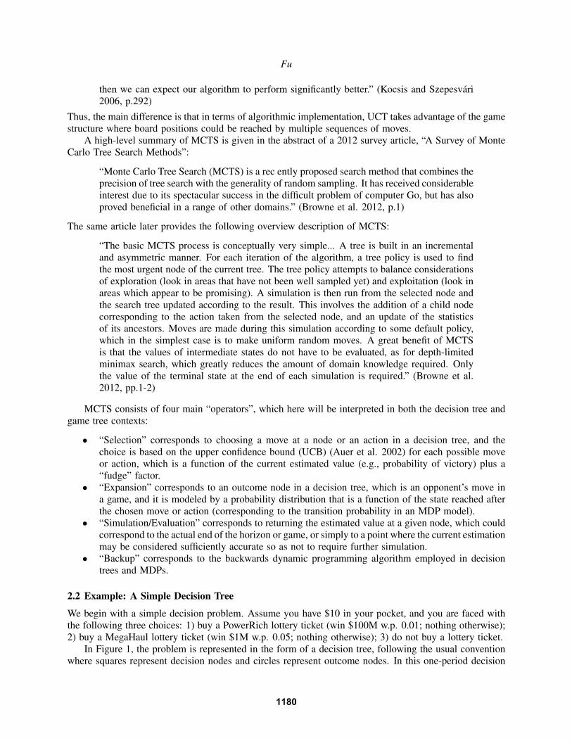
Assume henceforth that we are the “O” player. We begin by illustrating with two games that havealready seen three moves, 2 by our opponent and 1 by us, so it is our turn to make a move. The twodifferent board configurations are shown in Figure 3. For the first game, by symmetry there are just twounique moves for us to consider: corner or (non-corner) side. In this particular situation, following theoptimal policy above leads to an easy decision: corner move leads to a loss, and non-corner move leads toa draw; there is a unique “sample path” in both cases and thus no need to simulate. The trivial game treeand decision tree are given in Figures 4 and 5, respectively, with the game tree that allows non-optimalmoves shown in Figure 6.

×◦×

◦ × ×

Figure 3: Two tic-tac-toe board configurations to be considered.

×◦×

×◦×◦

loss (after next move)

×◦×◦

eventual draw

��

move 1 @@move 2

Figure 4: Game tree for 1st tic-tac-toe board configuration (assuming “greedy optimal” play), where notethat if opponent’s moves were completely randomized, “O” would have an excellent chance of winning!

2���

����

���

corner

©block

lose

PPPPPPPPPP

non-corner

©block

draw

Figure 5: Decision tree for 1st tic-tac-toe board configuration of Figure 3.

Now consider the other more interesting game configuration, the righthand side of Figure 3, wherethere are three unique moves available to us; without loss of generality, they can be the set of moves onthe top row. We need to evaluate the “value” of each of the three actions to determine which one to select.

1183

Fu

2���

����

���

corner

©���

����

��cornerlose

PPPPPPPPPnon-cornerwin

PPPPPPPPPP

non-corner

©����

����

�block

draw

PPPPPPPPPnon-blockwin

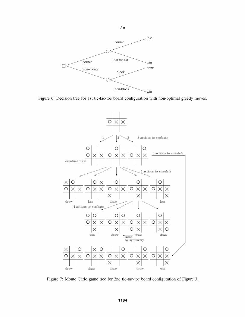
Figure 6: Decision tree for 1st tic-tac-toe board configuration with non-optimal greedy moves.

Figure 7: Monte Carlo game tree for 2nd tic-tac-toe board configuration of Figure 3.

1184

Fu

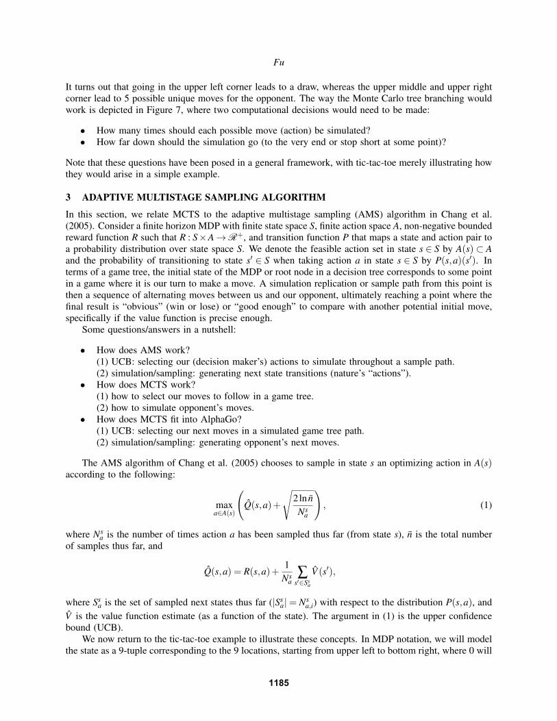
It turns out that going in the upper left corner leads to a draw, whereas the upper middle and upper rightcorner lead to 5 possible unique moves for the opponent. The way the Monte Carlo tree branching wouldwork is depicted in Figure 7, where two computational decisions would need to be made:

• How many times should each possible move (action) be simulated?• How far down should the simulation go (to the very end or stop short at some point)?

Note that these questions have been posed in a general framework, with tic-tac-toe merely illustrating howthey would arise in a simple example.

3 ADAPTIVE MULTISTAGE SAMPLING ALGORITHM

In this section, we relate MCTS to the adaptive multistage sampling (AMS) algorithm in Chang et al.(2005). Consider a finite horizon MDP with finite state space S, finite action space A, non-negative boundedreward function R such that R : S×A→R+, and transition function P that maps a state and action pair toa probability distribution over state space S. We denote the feasible action set in state s ∈ S by A(s)⊂ Aand the probability of transitioning to state s′ ∈ S when taking action a in state s ∈ S by P(s,a)(s′). Interms of a game tree, the initial state of the MDP or root node in a decision tree corresponds to some pointin a game where it is our turn to make a move. A simulation replication or sample path from this point isthen a sequence of alternating moves between us and our opponent, ultimately reaching a point where thefinal result is “obvious” (win or lose) or “good enough” to compare with another potential initial move,specifically if the value function is precise enough.

Some questions/answers in a nutshell:

• How does AMS work?(1) UCB: selecting our (decision maker’s) actions to simulate throughout a sample path.(2) simulation/sampling: generating next state transitions (nature’s “actions”).

• How does MCTS work?(1) how to select our moves to follow in a game tree.(2) how to simulate opponent’s moves.

• How does MCTS fit into AlphaGo?(1) UCB: selecting our next moves in a simulated game tree path.(2) simulation/sampling: generating opponent’s next moves.

The AMS algorithm of Chang et al. (2005) chooses to sample in state s an optimizing action in A(s)according to the following:

maxa∈A(s)

(Q(s,a)+

√2ln nNs

a

), (1)

where Nsa is the number of times action a has been sampled thus far (from state s), n is the total number

of samples thus far, and

Q(s,a) = R(s,a)+1

Nsa

∑s′∈Ss

a

V (s′),

where Ssa is the set of sampled next states thus far (|Ss

a|= Nsa,i) with respect to the distribution P(s,a), and

V is the value function estimate (as a function of the state). The argument in (1) is the upper confidencebound (UCB).

We now return to the tic-tac-toe example to illustrate these concepts. In MDP notation, we will modelthe state as a 9-tuple corresponding to the 9 locations, starting from upper left to bottom right, where 0 will

1185

Fu

correspond to blank, 1 = X, and 2 = O; thus, (0,0,1,0,2,0,1,0,0) and (0,0,0,2,1,1,0,0,0) correspond to thestates of the two board configurations of Figure 3. Actions will simply be represented by the 9 locations,with the feasible action space the obvious remainder set of the components of the space that are still 0,i.e., {1,2,4,6,8,9} and {1,2,3,7,8,9} for the two board configurations of Figure 3. This is not necessarilythe best state representation (e.g., if we’re trying to detect certain structure or symmetries). If the learningalgorithm is working how we would like it to work ideally, it should converge to the degenerate distributionthat chooses with probability one the optimal action, which can be easily determined in this simple game.

4 GO AND MCTS

Go is the most popular two-player board game in East Asia, tracing its origins to China more than2,500 years ago. According to Wikipedia, Go is also thought to be the oldest board game still playedtoday. Since the size of the board is 19×19, as compared to 8×8 for a chess board, the number ofboard configurations for Go far exceeds that for chess, with estimates at around 10170 possibilities, puttingit a googol (no pun intended) times beyond that of chess and exceeding the number of atoms in theuniverse (https://googleblog.blogspot.nl/2016/01/alphago-machine-learning-game-go.html). Intuitively, theobjective is to have “captured” the most territory by the end of the game, which occurs when both playersare unable to move or choose not to move, at which point the winner is declared as the player with thehighest score, calculated according to certain rules. Unlike chess, the player with the black (dark) piecesmoves first in Go, but same as chess, there is supposed to be a slight first-mover advantage (which isactually compensated by a fixed number of points decided prior to the start of the game).

Perhaps the closest game in the Western world to Go is Othello, which like chess is played on an 8×8board, and like Go has the player with the black pieces moving first. Similar to Go, there is also a “flanking”objective, but with far simpler rules. The number of legal positions is estimated at less than 1028, nearly agoogol and a half times less than the estimated number of possible Go board positions. As a result of thefar smaller number of possibilities, traditional exhaustive game tree search (which could include heuristicprocedures such as genetic algorithms and other evolutionary approaches leading to a pruning of the tree)can in principle handle the game of Othello, so that brute-force programs with enough computing powerwill easily beat any human. More intelligent programs can get by with far less computing (so that theycan be implemented on a laptop or smartphone), but the point is that complete solvability is within therealm of computational tractability given today’s available computing power, whereas such an approach isdoomed to failure for the game of Go, merely due to the 19×19 size of the board.

Similarly, IBM Deep Blue’s victory (by 3 1/2 to 2 1/2 points) over the chess world champion GarryKasparov in 1997 was more of an example of sheer computational power than true artificial intelligence,as reflected by the program being referred to as “the primitive brute force-based Deep Blue” in thecurrent Wikipedia account of the match. Again, traditional game tree search was employed, whichbecomes impractical for Go, as alluded to earlier. The realization that traversing the entire game tree wascomputationally infeasible for Go meant that new approaches were required, leading to a fundamentalparadigm shift, the main components being Monte Carlo sampling (or simulation of sample paths) and valuefunction approximation, which are the basis of simulation-based approaches to solving Markov decisionprocesses (Chang et al. 2007), which are also addressed by neuro-dynamic programming (Bertsekasand Tsitsiklis 1996); approximate (or adaptive) dynamic programming (Powell 2010); and reinforcementlearning (Sutton and Barto 1998). However, the setting for these approaches is that of a single decisionmaker tackling problems involving a sequence of decision epochs with uncertain payoffs and/or transitions.The game setting adapted these frameworks by modeling the uncertain transitions – which could be viewedas the actions of “nature” – as the action of the opposing player. As a consequence, to put the game settinginto the MDP setting required modeling the state transition probabilities as a distribution over the actionsof the opponent. Thus, as we shall describe later, AlphaGo employs two deep neural networks: one forvalue function approximation and the other for policy approximation, used to sample opponent moves.

1186

Fu

2 8 J A N U A R Y 2 0 1 6 | V O L 5 2 9 | N A T U R E | 4 8 5

ARTICLE RESEARCH

sampled state-action pairs (s, a), using stochastic gradient ascent to maximize the likelihood of the human move a selected in state s

∆σσ

∝∂ ( | )∂

σp a slog

We trained a 13-layer policy network, which we call the SL policy network, from 30 million positions from the KGS Go Server. The net-work predicted expert moves on a held out test set with an accuracy of 57.0% using all input features, and 55.7% using only raw board posi-tion and move history as inputs, compared to the state-of-the-art from other research groups of 44.4% at date of submission24 (full results in Extended Data Table 3). Small improvements in accuracy led to large improvements in playing strength (Fig. 2a); larger networks achieve better accuracy but are slower to evaluate during search. We also trained a faster but less accurate rollout policy pπ(a|s), using a linear softmax of small pattern features (see Extended Data Table 4) with weights π; this achieved an accuracy of 24.2%, using just 2 µs to select an action, rather than 3 ms for the policy network.

Reinforcement learning of policy networksThe second stage of the training pipeline aims at improving the policy network by policy gradient reinforcement learning (RL)25,26. The RL policy network pρ is identical in structure to the SL policy network,

and its weights ρ are initialized to the same values, ρ = σ. We play games between the current policy network pρ and a randomly selected previous iteration of the policy network. Randomizing from a pool of opponents in this way stabilizes training by preventing overfitting to the current policy. We use a reward function r(s) that is zero for all non-terminal time steps t < T. The outcome zt = ± r(sT) is the termi-nal reward at the end of the game from the perspective of the current player at time step t: +1 for winning and −1 for losing. Weights are then updated at each time step t by stochastic gradient ascent in the direction that maximizes expected outcome25

∆ρρ

∝∂ ( | )

∂ρp a s

zlog t t

t

We evaluated the performance of the RL policy network in game play, sampling each move ∼ (⋅| )ρa p st t from its output probability distribution over actions. When played head-to-head, the RL policy network won more than 80% of games against the SL policy network. We also tested against the strongest open-source Go program, Pachi14, a sophisticated Monte Carlo search program, ranked at 2 amateur dan on KGS, that executes 100,000 simulations per move. Using no search at all, the RL policy network won 85% of games against Pachi. In com-parison, the previous state-of-the-art, based only on supervised

Figure 1 | Neural network training pipeline and architecture. a, A fast rollout policy pπ and supervised learning (SL) policy network pσ are trained to predict human expert moves in a data set of positions. A reinforcement learning (RL) policy network pρ is initialized to the SL policy network, and is then improved by policy gradient learning to maximize the outcome (that is, winning more games) against previous versions of the policy network. A new data set is generated by playing games of self-play with the RL policy network. Finally, a value network vθ is trained by regression to predict the expected outcome (that is, whether

the current player wins) in positions from the self-play data set. b, Schematic representation of the neural network architecture used in AlphaGo. The policy network takes a representation of the board position s as its input, passes it through many convolutional layers with parameters σ (SL policy network) or ρ (RL policy network), and outputs a probability distribution ( | )σp a s or ( | )ρp a s over legal moves a, represented by a probability map over the board. The value network similarly uses many convolutional layers with parameters θ, but outputs a scalar value vθ(s′) that predicts the expected outcome in position s′.

Regr

essi

on

Cla

ssifi

catio

nClassification

Self Play

Policy gradient

a b

Human expert positions Self-play positions

Neural netw

orkD

ata

Rollout policy

pS pV pV�U (a⎪s) QT (s′)pU QT

SL policy network RL policy network Value network Policy network Value network

s s′

Figure 2 | Strength and accuracy of policy and value networks. a, Plot showing the playing strength of policy networks as a function of their training accuracy. Policy networks with 128, 192, 256 and 384 convolutional filters per layer were evaluated periodically during training; the plot shows the winning rate of AlphaGo using that policy network against the match version of AlphaGo. b, Comparison of evaluation accuracy between the value network and rollouts with different policies.

Positions and outcomes were sampled from human expert games. Each position was evaluated by a single forward pass of the value network vθ, or by the mean outcome of 100 rollouts, played out using either uniform random rollouts, the fast rollout policy pπ, the SL policy network pσ or the RL policy network pρ. The mean squared error between the predicted value and the actual game outcome is plotted against the stage of the game (how many moves had been played in the given position).

15 45 75 105 135 165 195 225 255 >285Move number

0.10

0.15

0.20

0.25

0.30

0.35

0.40

0.45

0.50

Mea

n sq

uare

d er

ror

on e

xper

t gam

es

Uniform random rollout policyFast rollout policyValue networkSL policy networkRL policy network

50 51 52 53 54 55 56 57 58 59Training accuracy on KGS dataset (%)

0

10

20

30

40

50

60

70128 filters192 filters256 filters384 filters

Alp

haG

o w

in ra

te (%

)

a b

© 2016 Macmillan Publishers Limited. All rights reserved

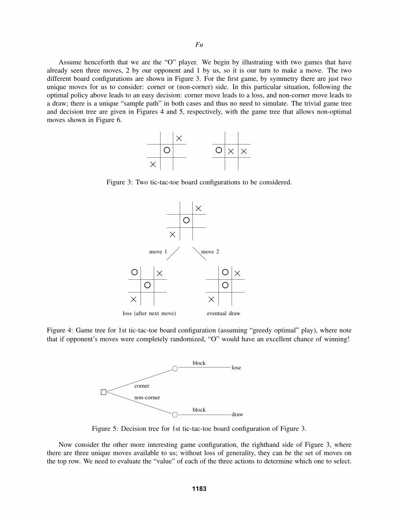
Figure 8: AlphaGo’s two deep neural networks (Adapted by permission from Macmillan Publishers Ltd.:Nature, Figure 1b, Silver et al. 2016, copyright 2016).

In March 2016 in Seoul, Korea, Google DeepMind’s computer program AlphaGo defeated the reigninghuman world champion Go player Lee Sedol 4 games to 1, representing yet another advance in artificialintelligence (AI) arguably more impressive than previous victories by computer programs in chess (IBM’sDeep Blue) and Jeopardy (IBM’s Watson), due to the sheer size of the problem. A little over a year later,in May 2017 in Wuzhen, China, at “The Future of Go Summit,” a gathering of the world’s leading Goplayers, AlphaGo cemented its reputation as the planet’s best by defeating Chinese Go Grandmaster andworld number one (only 19 years old) Ke Jie (three games to none). An interesting postscript to the matchwas Ke Jie’s remarks two months later (July 2017), as quoted on the DeepMind Web site blog (DeepMind2018): “After my match against AlphaGo, I fundamentally reconsidered the game, and now I can see thatthis reflection has helped me greatly. I hope all Go players can contemplate AlphaGo’s understanding ofthe game and style of thinking, all of which is deeply meaningful. Although I lost, I discovered that thepossibilities of Go are immense and that the game has continued to progress.”

Before describing AlphaGo’s two deep neural networks that are trained using MCTS, a little backgroundon DeepMind, the London-based artificial intelligence (AI) company founded in 2010 by Demis Hassabis,Shane Legg and Mustafa Suleyman. DeepMind built its reputation on the use of deep neural networks forAI applications, most notably video games, and was acquired by Google in 2014 for $500M. David Silver,the DeepMind Lead Researcher for AlphaGo and lead author on all three articles (Silver et al. 2016; Silveret al. 2017ab) is quoted on the AlphaGo movie Web page (AlphaGo Movie 2017): “The Game of Go isthe holy grail of artificial intelligence. Everything we’ve ever tried in AI, it just falls over when you trythe game of Go.” However, the company emphasizes that it focuses on building learning algorithms thatcan be generalized, just as AlphaGo Zero and AlphaZero developed from AlphaGo. In addition to deepneural networks and reinforcement learning, it develops other systems neuroscience-inspired models.

AlphaGo’s two neural networks are depicted in Figure 8:

1187

Fu

2���

����

����

��

1

D

2 ©���

W

��� D

���

L

2PPP

D

3

©

PPPPPPPPPP ��� D

DPPP DQQQ D

@@@

W

���W

DPPP DQQQ D

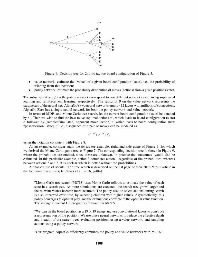
Figure 9: Decision tree for 2nd tic-tac-toe board configuration of Figure 3.

• value network: estimate the “value” of a given board configuration (state), i.e., the probability ofwinning from that position;

• policy network: estimate the probability distribution of moves (actions) from a given position (state).

The subscripts σ and ρ on the policy network correspond to two different networks used, using supervisedlearning and reinforcement learning, respectively. The subscript θ on the value network represents theparameters of the neural net. AlphaGo’s two neural networks employ 12 layers with millions of connections.AlphaGo Zero has a single neural network for both the policy network and value network.

In terms of MDPs and Monte Carlo tree search, let the current board configuration (state) be denotedby s∗. Then we wish to find the best move (optimal action) a∗, which leads to board configuration (state)s, followed by (sampled/simulated) opponent move (action) a, which leads to board configuration (new“post-decision” state) s′, i.e., a sequence of a pair of moves can be modeled as

s∗ a∗−→ s a−→ s′,

using the notation consistent with Figure 8.As an example, consider again the tic-tac-toe example, righthand side game of Figure 3, for which

we derived the Monte Carlo game tree as Figure 7. The corresponding decision tree is shown in Figure 9,where the probabilities are omitted, since these are unknown. In practice the “outcomes” would also beestimated. In this particular example, action 3 dominates action 1 regardless of the probabilities, whereasbetween actions 2 and 3, it is unclear which is better without the probabilities.

AlphaGo’s use of Monte Carlo tree search is described on the 1st page of their 2016 Nature article inthe following three excerpts (Silver et al. 2016, p.484):

”Monte Carlo tree search (MCTS) uses Monte Carlo rollouts to estimate the value of eachstate in a search tree. As more simulations are executed, the search tree grows larger andthe relevant values become more accurate. The policy used to select actions during searchis also improved over time, by selecting children with higher values. Asymptotically, thispolicy converges to optimal play, and the evaluations converge to the optimal value function.The strongest current Go programs are based on MCTS...

“We pass in the board position as a 19 × 19 image and use convolutional layers to constructa representation of the position. We use these neural networks to reduce the effective depthand breadth of the search tree: evaluating positions using a value network, and samplingactions using a policy network.

“Our program AlphaGo efficiently combines the policy and value networks with MCTS.”

1188

Fu

Figure 8 shows the corresponding p(a|s) for the policy neural network that is used to simulate theopponent’s moves and the value function v(s′) that estimates the value of a board configuration (state) usingthe value neural network. The latter could be used in the following way: if a state is reached where thevalue is known with sufficient precision, then stop there and start the backwards dynamic programming;else, simulate further by following the UCB prescription for the next move to explore.

The objective is to effectively and efficiently (through appropriate parametrization) approximate thevalue function approximation and represent the opposing player’s moves as a probability distribution, whichdegenerates to a deterministic policy if the game is easily solved to completion assuming the opponentplays “optimally.” However, at the core of these lies the Monte Carlo sampling of game trees or what ourcommunity would call the simulation of sample paths. Although the game is completely deterministic,unlike other games of chance such as those involving the dealing of playing cards (e.g., bridge and poker), thesheer astronomical number of possibilities precludes the use of brute-force enumeration of all possibilities,thus leading to the adoption of randomized approaches. This in itself is not new, even for games, but theGo-playing programs have transformed this from simple coin flips for search (which branch to follow)to the evaluation of a long sequence of alternating moves, with the opponent modeled by a probabilitydistribution over possible moves in the given reached configuration. In the framework of MDPs, Go can beviewed as a finite-horizon problem where the objective is to maximize an expected reward (the territorialadvantage) or the probability of victory, where the randomness or uncertainty comes from two sources: thestate transitions, which depend on the opposing player’s move, and the single-stage reward, which couldbe territorial (actual perceived gain) or strategic (an increase or decrease in the probability of winning), asalso reflected in the estimated value after the opponent’s move.

Coda: MCTS for Chess

For chess, AlphaZero uses MCTS to search 80K positions per second, which sounds like a lot. However,Stockfish, considered in 2017 by many to be the best computer chess-playing program (way better than anyhuman that has ever lived) considers about 70M positions per second, i.e., nearly three orders of magnitudemore, and yet AlphaZero did not lose a single game to Stockfish in their December 2017 100-game match(28 wins, 72 draws). “Instead of an alpha-beta search with domain-specific enhancements, AlphaZero usesa general-purpose Monte-Carlo tree search (MCTS) algorithm.” (Silver et al. 2018, p.3)

5 CONCLUSIONS

Monte Carlo tree search (MCTS) provides the foundation for training the “deep” neural networks ofAlphaGo, as well as the single neural network engine for its successor AlphaZero. The roots of MCTS arecontained in the more general adaptive multi-stage sampling algorithms for MDPs published by Chang et al.(2005) in Operations Research, where dynamic programming (backward induction) is used to estimate thevalue function in an MDP. A game tree can be viewed as a decision tree (simplified MDP) with the opponentin place of “nature” in the model. In AlphaZero, both the policy and value networks are contained in asingle neural net, which makes it suitable to play against itself when the net is trained for playing both sidesof the game. Thus, an important takeaway message to be conveyed is that OR played an unheralded role,as the MCTS algorithm is based on the UCB algorithm for MDPs, with dynamic programming (backwardinduction) used to calculate/estimate the value function in an MDP (game tree, viewed as a decision treewith the opponent in place of “nature” in the model).

One caveat emptor when reading the literature on MCTS: Most of the papers in the bandit literatureassume that the support of the reward is [0,1] (or {0,1} in the case of Bernoulli rewards), which essentiallytranslates to knowing the support. Depending on the application, this may not be a reasonable assumption.Estimating the variance is probably easier, if not more intuitive, than estimating the support, and this isthe approach in the work of Li et al. (2018) described further below.

1189

Fu

The ML/AI community mainly views MCTS as a tool that can be applied to a wide variety of domains,so the focus is generally on the model that is used rather than the training method, i.e., the emphasis ison choosing the neural network architecture or regression model. Far less attention has been paid on thealgorithmic aspects of MCTS. One direction that has started to be investigated is the use of ranking &selection (R/S) techniques for the selection of which path to sample next rather than traditional multi-armedbandit models, which tend to emphasize exploitation over exploration, e.g., leading to sampling the optimalmove/action exponentially more often than the others. Similar to R/S, in MCTS, there is also the differencebetween choosing which moves to sample further versus which move to declare the “best” to play at a givenpoint in time. In fact, in his original paper introducing MCTS, Coulom himself mentions this alternative,viz., “Optimal schemes for the allocation of simulations in discrete stochastic optimization could also beapplied to Monte-Carlo tree search” (Coulom 2006, p.74), where one of the cited papers is the OCBApaper by Chen et al. (2000).

The distinction between simulation allocation and the final choice of best alternative in R/S is treatedrigorously in a stochastic control framework in Peng et al. (2018), and again is noted by Coulom (Coulom2006, p.75), viz.,

“Although they provide interesting sources of inspiration, the theoretical frameworks of n-armed bandit problems and discrete stochastic optimization do not fit Monte-Carlo tree searchperfectly. We provide two reasons: First, and most importantly, n-armed bandit algorithmsand stochastic optimization assume stationary distributions of evaluations, which is not thecase when searching recursively. Second, in n-armed bandit problems, the objective is toallocate simulations in order to minimize the number of selections of non-optimal movesduring simulations. This is not the objective of Monte-Carlo search, since it does not matterwhen bad moves are searched, as long a good move is finally selected.“The field of discrete stochastic optimization is more interesting in this respect, since itsobjective is to optimize the final decision, either by maximizing the probability of selectingthe best move, or by maximizing the expected value of the final choice. This maximizingprinciple should be the objective at the root of the tree, but not in internal nodes, where thetrue objective in Monte-Carlo search is to estimate the value of the node as accurately aspossible. For instance, let us take Chen’s formula, with the choice between two moves, andlet the simulations of these two moves have the same variance, then the optimal allocationconsists in exploring both moves equally more deeply, regardless of their estimated values.This does indeed optimize the probability of selecting the best move, but is not at all whatwe wish to do inside a search tree: the best move should be searched more than the othermove, since it will influence the backed-up value more.”

“Chen’s formula” referenced in the 2nd paragraph is the optimal computing budget allocation (OCBA)formula of Chun-Hung Chen and his collaborators (Chen et al. 2000). In the MDP setting, a recentwork on incorporating OCBA in place of UCB into MCTS is Li et al. (2018), which considers the moregeneral non-game framework of MDPs. In many applications beyond games, they incorporate severalcharacteristics that MCTS generally ignores: (i) support of (period) reward(s) is unknown (and possiblyunbounded), requiring estimation; (ii) inherent stochasticity in the rewards and in the actual transitions. Liet al. (2018) also note that the objective at the first stage may differ from that of subsequent stages, sinceat the first stage the ultimate goal is to determine the “best” action, whereas in subsequent stages the goalis to estimate a value function. Also, with parallel computing, it may actually make more sense to usebatch mode rather than fully sequential allocation algorithms.

The game of tic-tac-toe is a nice illustrative example for MCTS, due to its simplicity, and it is usedin the first chapter of Sutton and Barto (1998) to introduce the reader to many of the more general issuesin reinforcement learning. To allow experimenting with MCTS firsthand for the tic-tac-toe example, aJava-based demo program is available online at the author’s Web page:

1190

Fu

https://terpconnect.umd.edu/∼mfu/demo (programming by Uro Lyi, a University of Maryland undergraduatemath/CS major). Two other games that would be good candidates for applying MCTS and comparing it ina more meaningful way with other approaches are Othello (mentioned earlier in the introduction) and “Fivein a Row” (aka Gomoku or Gobang, I recently found out; see Wikipedia), because these could probably stillbe programmed and implemented without the equivalent of supercomputers (or tensor processing units) forthe (value and policy) function approximations, which in AlphaGo and AlphaZero require the deep neuralnets. Backgammon is another game, differing from the previously mentioned ones in that randomness isan inherent part, that would also be a good test setting for MCTS, and the program TD-gammon (Tesauro1995) was an early success story for the approach of what is now known more generally as reinforcementlearning, neuro-dynamic programming, or approximate dynamic programming. Other games that areinherently random such as bridge and poker would be formidable challenges for AlphaZero to extendsits reach, and it would be very interesting to see it go up against the AI systems DeepStack (Moravcıket al. 2017) or Libratus (Brown and Sandholm 2018), which recently decisively bested four of the world’sbest poker players, becoming the “first AI to beat professional poker players at heads-up, no-limit TexasHold’em.” Apparently, the strategies that were developed followed more traditional AI approaches and didnot use MCTS, but one possibility might be to convert the random game into a partially observable MDP(POMDP) and see if MCTS could be applied to the augmented state. Finally, as of this writing, computerbridge programs have not yet achieved the same level of success.

ACKNOWLEDGMENTS

This work was supported in part by the National Science Foundation (NSF) under Grant CMMI-1434419.

REFERENCESMCTS Tic-Tac-Toe Demo Program. 2020. https://terpconnect.umd.edu/∼mfu/demo/index.html. Accessed

August 5, 2020.AlphaGo Movie. 2017. https://www.alphagomovie.com. Accessed August 5, 2020.Auer, P., N. Cesa-Bianchi, and P. Fisher. 2002. “Finite-Time Analysis of the Multiarmed Bandit Problem”.

Machine Learning 47:235–256.Bertsekas, D. P., and J. N. Tsitsiklis. 1996. Neuro-Dynamic Programming. Belmont, MA: Athena Scientific.Broadie, M., and P. Glasserman. 1996. “Estimating Security Price Derivatives Using Simulation”. Man-

agement Science 42(2):269–285.Brown, N., and T. Sandholm. 2018. Superhuman AI for Heads-Up No-Limit Poker: Libratus beats top

professionals. Science 359(6374):418–424.Browne, C., E. Powley, D. Whitehouse, S. Lucas, P. I. Cowling, P. Rohlfshagen, S. Tavener, D. Perez,

S. Samothrakis, and S. Colton. 2012. “A Survey of Monte Carlo Tree Search Methods”. IEEE Transactionson Computational Intelligence and AI in Games 4(1):1–49.

Chang, H. S., M. C. Fu, J. Hu, and S. I. Marcus. 2005. “An Adaptive Sampling Algorithm for SolvingMarkov Decision Processes”. Operations Research 53(1):126–139.

Chang, H. S., M. C. Fu, J. Hu, and S. I. Marcus. 2007. Simulation-based Algorithms for Markov DecisionProcesses. New York: Springer.

Chang, H. S., M. C. Fu, J. Hu, and S. I. Marcus. October 2016. “Google Deep Mind’s AlphaGo”. OR/MSToday:24–29.

Chen, C.-H., J. Lin, E. Yucesan, and S. E. Chick. 2000. “Simulation Budget Allocation for FurtherEnhancing the Efficiency of Ordinal Optimization.” Journal of Discrete Event Dynamic Systems:Theory and Applications 10(3):251-270,

Coulom, R. 2006. “Efficient Selectivity and Backup Operators in Monte-Carlo Tree Search”. In Computersand Games: CG 2006. Lecture Notes in Computer Science, vol 4630. edited by H. J. van den Herik,P. Ciancarini, and H. H. L. M. Donkers, 72–83, Berlin, Germany: Springer.

DeepMind 2018. https://deepmind.com/research/alphago. Accessed May 7, 2017 and August 5, 2020.

1191

Fu

Fu, M. C., editor. 2015. Handbook on Simulation Optimization. New York: Springer.Fu, M. C.. 2016. “AlphaGo and Monte Carlo Tree Search: The Simulation Optimization Perspective”.

In Proceedings of the 2016 Winter Simulation Conference, edited by T. M. K. Roeder, P. I. Frazier,R. Szechtman, E. Zhou, T. Huschka, and S. E. Chick, 659–670. Piscataway, NJ: IEEE.

Fu, M. C.. 2017. “Markov Decision Processes, AlphaGo, and Monte Carlo Tree Search: Back to the Future”.Chapter 4 in Tutorials in Operations Research, edited by R. Batta and J. Peng, 68–88. Catonsville,MD: INFORMS.

Fu, M. C. 2018. “Monte Carlo Tree Search: A Tutorial”. In Proceedings of the 2018 Winter SimulationConference, edited by M. Rabe, A. A. Juan, N. Mustafee, A. Skoogh, S. Jain, and B. Johansson,222–236. Piscataway, NJ: IEEE.

Fu, M. C., “Simulation-based Algorithms for Markov Decision Processes: Monte Carlo Tree Search fromAlphaGo to AlphaZero”. Asia-Pacific Journal of Operational Research, Vol.36, No.6, 2019.

Gass, S.I., and M.C. Fu, editors. 2013. Encyclopedia of Operations Research and Management Science.3rd ed. (2 volumes). New York: Springer.

Kahneman, D., and A. Tversky. 1979. “Prospect Theory: An Analysis of Decision Under Risk”. Econometrica47(2):263–291.

Kocsis, L., and C. Szepesvari. 2006. “Bandit based Monte-Carlo Planning”. In Machine Learning:ECML 2006. Lecture Notes in Computer Science, vol 4212. edited by J. Furnkranz, T. Scheffer,and M. Spiliopoulou, 282–293, Berlin, Germany: Springer.

Li, Y., M. C. Fu and J. Xu. 2019. “Monte Carlo Tree Search with Optimal Computing Budget Allocation”.Proceedings of the IEEE Conference on Decision and Control (journal version under review at IEEETransactions on Automatic Control, 2020).

Moravcık, M., M. Schmid, N. Burch, V. Lisy, D. Morrill, N. Bard, T. Davis, K. Waugh, M. Johanson,and M. Bowling. 2017. DeepStack: Expert-Level Artificial Intelligence in Heads-Up No-Limit Poker.Science 356 508–513.

Peng, Y., C.-H. Chen, E. K. P. Chong, and M. C. Fu. 2018. “Ranking and Selection as Stochastic Control”.IEEE Transactions on Automatic Control 63(8):2359-2373.

Powell, W. B. 2010. Approximate Dynamic Programming. 2nd ed. New York: Wiley.Prashanth, L. A., C. Jie, M. C. Fu, S. I. Marcus, and C. Szepesvari. 2016. “Cumulative Prospect Theory Meets

Reinforcement Learning: Prediction and Control”. In ICML’16: Proceedings of the 33rd InternationalConference on Machine Learning, edited by M. F. Balcan and K. Q. Weinberger, 1406–1415. NewYork: JMLR.org.

Schaefer, S. 2002. “MathRec Solutions (Tic-Tac-Toe).” Mathematical Recreations.http://www.mathrec.org/old/2002jan/solutions.html. Accessed July 16, 2020.

Silver, D., A. Huang, Aja, C. Maddison, A. Guez, L. Sifre, G. van den Driessche, J. Schrittwieser, I.Antonoglou, V. Panneershelvam, M. Lanctot, S. Dieleman, D. Grewe, J. Nham, N. Kalchbrenner, I.Sutskever, T. Lillicrap, M. Leach, K. Kavukcuoglu, T. Graepel, and D. Hassabis. 2016. ”Mastering theGame of Go with Deep Neural Networks and Tree Search”. Nature 529 (28 Jan):484–503.

Silver, D., J. Schrittwieser, K. Simonyan, I. Antonoglou, A. Huang, A. Guez, T. Hubert, L. Baker, M. Lai,A. Bolton, Y. Chen, T. Lillicrap, F. Hui, L. Sifre, G. van den Driessche, T. Graepel, and D. Hassabis.2017. Mastering the Game of Go without Human Knowledge. Nature 550 (19 Oct):354–359.

Silver, D., Thomas Hubert, Julian Schrittwieser, Ioannis Antonoglou, Matthew Lai, Arthur Guez, MarcLanctot, Laurent Sifre, Dharshan Kumaran, Thore Graepel, Timothy Lillicrap, Karen Simonyan, DemisHassabis. 2018. A general reinforcement learning algorithm that masters chess, shogi, and Go throughself-play. Science 362:1140–1144.

Sutton, R. S., and A. G. Barto. 1998. Reinforcement Learning: An Introduction. Cambridge: MIT Press.Tesauro, G. 1995. Temporal Difference Learning and TD-gammon. Communications of the ACM 38(3):58–

68.

1192

Fu

AUTHOR BIOGRAPHY

MICHAEL C. FU holds the Smith Chair of Management Science in the Robert H. Smith School ofBusiness, with a joint appointment in the Institute for Systems Research and affiliate faculty appointmentin the Department of Electrical and Computer Engineering, A. James Clark School of Engineering, all atthe University of Maryland, College Park, where he has been since 1989. His research interests includestochastic gradient estimation, simulation optimization, and applied probability, with applications to man-ufacturing, supply chain management, and financial engineering. He has a Ph.D. in applied math fromHarvard and degrees in math and EECS from MIT. He is the co-author of the books, Conditional MonteCarlo: Gradient Estimation and Optimization Applications, which received the INFORMS SimulationSociety’s 1998 Outstanding Publication Award, and Simulation-Based Algorithms for Markov DecisionProcesses, and has also edited/co-edited four volumes: Perspectives in Operations Research, Advances inMathematical Finance, Encyclopedia of Operations Research and Management Science (3rd edition), andHandbook of Simulation Optimization. He attended his first WSC in 1988 and served as Program Chair forthe 2011 WSC. He received the INFORMS Simulation Society Distinguished Service Award in 2018. Hehas served as Program Director for the NSF Operations Research Program (2010–2012, 2015), ManagementScience Stochastic Models and Simulation Department Editor, and Operations Research Simulation AreaEditor. He is a Fellow of INFORMS and IEEE. His e-mail address is mfu@umd.edu, and his Web pageis https://www.rhsmith.umd.edu/directory/michael-fu.

1193