MT10 Ch8 solns

CHAPTER 8

STRATEGY AND GAME THEORY

These problems cover a variety of different concepts introduced in the chapter. They range in difficulty from the simplest exercise of finding the Nash equilibrium in a two-by-two matrix to characterizing equilibrium when players have continuous actions and payoffs with general functional forms. Practice with problems may be the primary way for students to master the material on game theory.

Comments on Problems

8.1 Provides practice in finding pure- and mixed-strategy Nash equilibria using a simple payoff matrix. The three-by-three payoff matrix makes the problem slightly harder than the simplest case of a two-by-two matrix. Although this problem points the student where to look for the mixed-strategy equilibrium, in other cases there may be many possibilities that need to be checked for mixed-strategy equilibria. In a game represented by a three-by-three matrix, each player has four combinations of two or more actions, and so there are 16 possible types of mixed-strategy equilibria to check. Software, called Gambit, has been developed that can solve for all the Nash equilibria of games the user specifies in extensive or normal form. Gambit is freely available on the Internet. It is easy to use, almost functioning as a “game-theory calculator.” One useful classroom exercise would be have students solve some of the problems on a game-theory problem set using Gambit, either alone or in teams.

McKelvey, R.D.; A.M. McLennan; and T. L. Turocy (2007) Gambit: Software Tools for Game Theory, Version 0.2007.01.30. http://econweb.tamu.edu/gambit

8.2 A slight generalization of payoffs in the Battle of the Sexes provides students with further practice in computing mixed-strategy Nash equilibria.

8.3 Provides practice in converting the payoff matrix for a simultaneous game into one for a sequential game. Illustrates the application of subgame-perfect equilibrium in the simple case of the famous Chicken game.

8.4 The problem provides practice in computing the Nash equilibrium in a game with continuous actions (similar to the Tragedy of the Commons in this chapter and in Chapter 15 with the Cournot game, except in this problem the best-

54

Chapter 8: Strategy and Game Theory

response functions are upward-sloping). Players’ best responses are computed using calculus, and the resulting equations are then solved simultaneously.

8.5 Asks students to solve for the mixed-strategy Nash equilibrium with a general number of players . The “punchline” to the problem that the blond is less likely to be approached as the number of males increases is a paradoxical result characteristic of such games. The problem is based on a scene in the Academy Award winning movie, A Beautiful Mind, about the life of John Nash, in which the Nash character discovers his equilibrium concept (the one scene in the movie that involves any game theory). If the classroom facilities allow, it is worthwhile to show students this scene (Scene 5: “Governing Dynamics”) when covering this problem.

8.6 Illustrates the folk theorem for finitely repeated games, similar to Example 8.7.

8.7 A simultaneous game of incomplete information providing practice in finding the Bayesian-Nash equilibrium. Similar to the Tragedy of the Commons in Example 8.9.

8.8 Asks students to solve for a hybrid perfect Bayesian equilibrium. Students may find the application interesting given the growth in popularity of poker on television, in particular Texas Hold ‘Em (to which the name “Blind Texan” in the problem is meant to be a tongue-in-cheek reference). In typical intermediate microeconomics courses, instructors will have only a short time to cover signaling games, and in such courses it would be perfectly reasonable to omit this problem, focusing exclusively on the simpler computations associated with separating and pooling equilibria. Two reasons to delve into hybrid equilibria if there is sufficient time, say in an advanced course with an extensive game theory component are a) games like Blind Texan do not have separating and pooling equilibria, only a hybrid one and b) the full power of Bayes Rule in a signaling game is only apparent with a hybrid equilibrium since the application of the rule with separating and pooling equilibria is fairly trivial.

Analytical Problems

8.9 Dominant strategies. Result can essentially be shown in a one-line proof linking the definitions of dominant strategy and Nash equilibrium. For instructors who prefer this style of problem, 8.10 provides another possible good choice. Other sources of “proof” type problems are generated by considering two-by-two games. For example, students can be asked to prove directly that a two-by-two game with no pure-strategy Nash equilibrium must have a mixed-strategy Nash equilibrium or that the two-by-two game must have an odd number of Nash equilibria generically (that is, if the game only has an even

55


number of Nash equilibria, a tiny change in the payoff will generate another one).

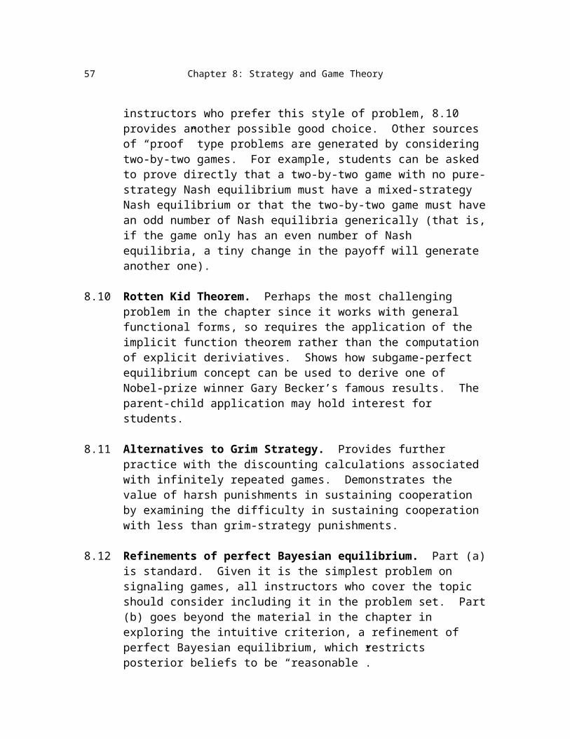
8.10 Rotten Kid Theorem. Perhaps the most challenging problem in the chapter since it works with general functional forms, so requires the application of the implicit function theorem rather than the computation of explicit deriviatives. Shows how subgame-perfect equilibrium concept can be used to derive one of Nobel-prize winner Gary Becker’s famous results. The parent-child application may hold interest for students.

8.11 Alternatives to Grim Strategy. Provides further practice with the discounting calculations associated with infinitely repeated games. Demonstrates the value of harsh punishments in sustaining cooperation by examining the difficulty in sustaining cooperation with less than grim-strategy punishments.

8.12 Refinements of perfect Bayesian equilibrium. Part (a) is standard. Given it is the simplest problem on signaling games, all instructors who cover the topic should consider including it in the problem set. Part (b) goes beyond the material in the chapter in exploring the intuitive criterion, a refinement of perfect Bayesian equilibrium, which restricts posterior beliefs to be “reasonable”.

Solutions

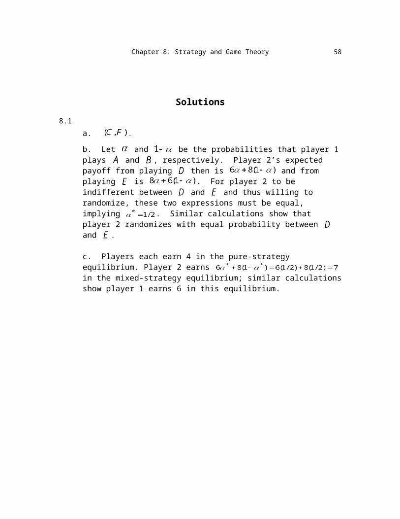
8.1

a. .

b. Let and be the probabilities that player 1 plays and , respectively. Player 2’s expected payoff from playing then is and from playing

is . For player 2 to be indifferent between and and thus willing to randomize, these two expressions must be equal, implying . Similar calculations show that player 2 randomizes with equal probability between and .

c. Players each earn 4 in the pure-strategy equilibrium. Player 2 earns in the mixed-strategy equilibrium; similar

calculations show player 1 earns 6 in this equilibrium.

56


d.

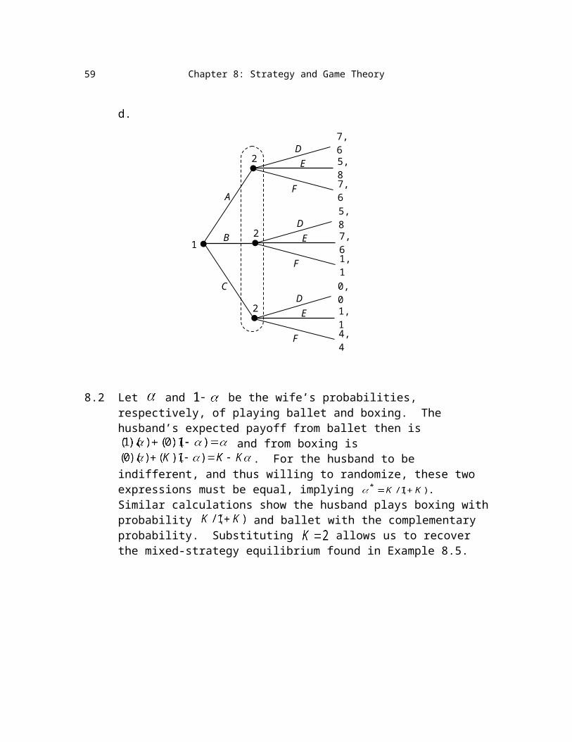
8.2 Let and be the wife’s probabilities, respectively, of playing ballet and boxing. The husband’s expected payoff from ballet then is

and from boxing is . For the husband to be indifferent, and thus willing to randomize, these two expressions must be equal, implying . Similar calculations show the husband plays boxing with probability and ballet with the complementary probability. Substituting allows us to recover the mixed-strategy equilibrium found in Example 8.5.

●

●2

1

A

B

C

D

E

F

7, 6

5, 8

7, 6

●2

D

E

F

5, 8

7, 6

1, 1

●2

D

E

F

0, 0

1, 1

4, 4

57


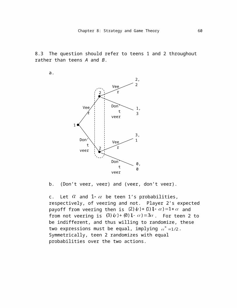
8.3 The question should refer to teens 1 and 2 throughout rather than teens A and B.

a.

b. (Don’t veer, veer) and (veer, don’t veer).

c. Let and be teen 1’s probabilities, respectively, of veering and not. Player 2’s expected payoff from veering then is and from not veering is . For teen 2 to be indifferent, and thus willing to randomize, these two expressions must be equal, implying . Symmetrically, teen 2 randomizes with equal probabilities over the two actions.

●

●2

1

Veer

Veer

Don’tveer

Don’tveer

2, 2

1, 3

●2

Veer

Don’tveer

3, 1

0, 0

58


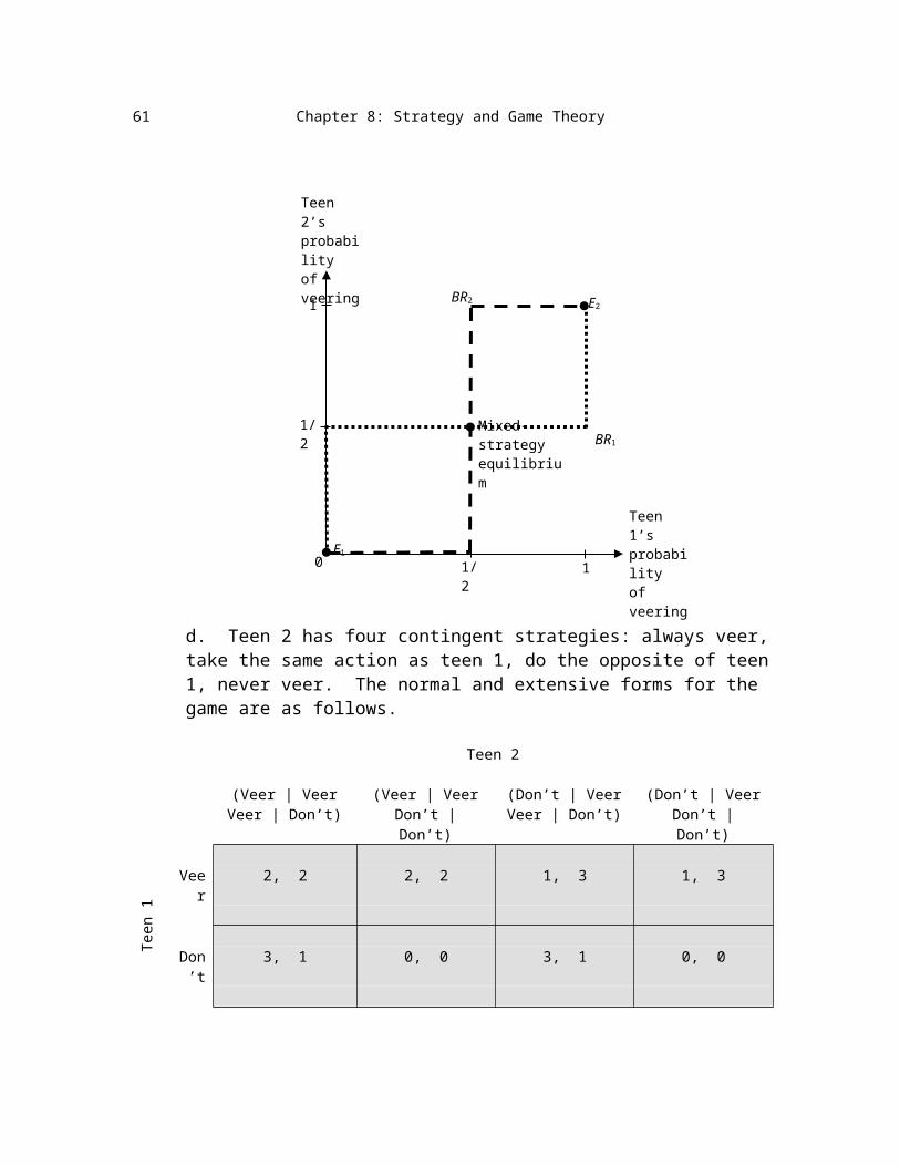
d. Teen 2 has four contingent strategies: always veer, take the same action as teen 1, do the opposite of teen 1, never veer. The normal and extensive forms for the game are as follows.

Teen 2

(Veer | VeerVeer | Don’t)

(Veer | VeerDon’t | Don’t)

(Don’t | VeerVeer | Don’t)

(Don’t | VeerDon’t | Don’t)

Tee

n 1 Veer 2, 2 2, 2 1, 3 1, 3

Don’t 3, 1 0, 0 3, 1 0, 0

0Teen 1’sprobabilityof veering

Teen 2’sprobabilityof veering

1/21

1/2

1BR2

BR1

●

●

●E1

E2

Mixed-strategyequilibrium

59


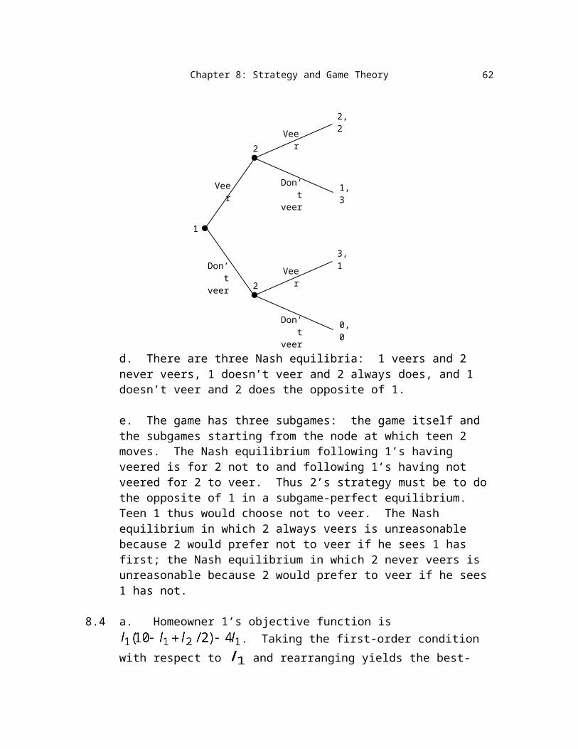
d. There are three Nash equilibria: 1 veers and 2 never veers, 1 doesn’t veer and 2 always does, and 1 doesn’t veer and 2 does the opposite of 1.

e. The game has three subgames: the game itself and the subgames starting from the node at which teen 2 moves. The Nash equilibrium following 1’s having veered is for 2 not to and following 1’s having not veered for 2 to veer. Thus 2’s strategy must be to do the opposite of 1 in a subgame-perfect equilibrium. Teen 1 thus would choose not to veer. The Nash equilibrium in which 2 always veers is unreasonable because 2 would prefer not to veer if he sees 1 has first; the Nash equilibrium in which 2 never veers is unreasonable because 2 would prefer to veer if he sees 1 has not.

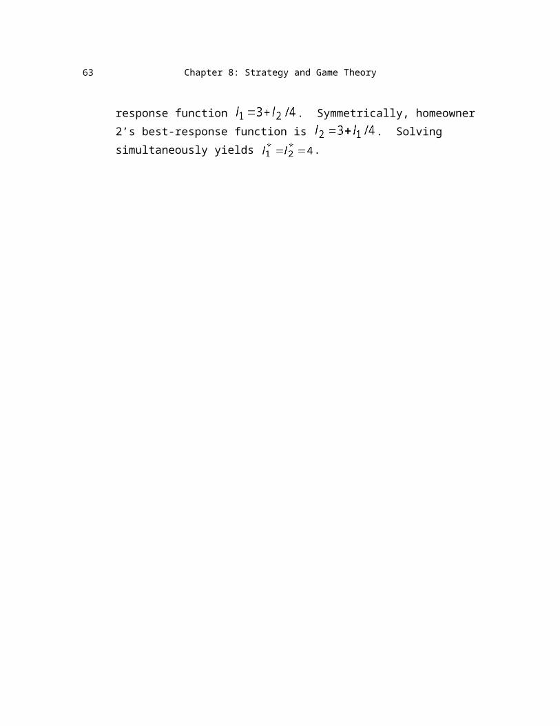
8.4 a. Homeowner 1’s objective function is . Taking the first-order condition with respect to and rearranging yields the best-response function . Symmetrically, homeowner 2’s best-response function is

. Solving simultaneously yields .

●

●2

1

Veer

Veer

Don’tveer

Don’tveer

2, 2

1, 3

●2

Veer

Don’tveer

3, 1

0, 0

60


b.

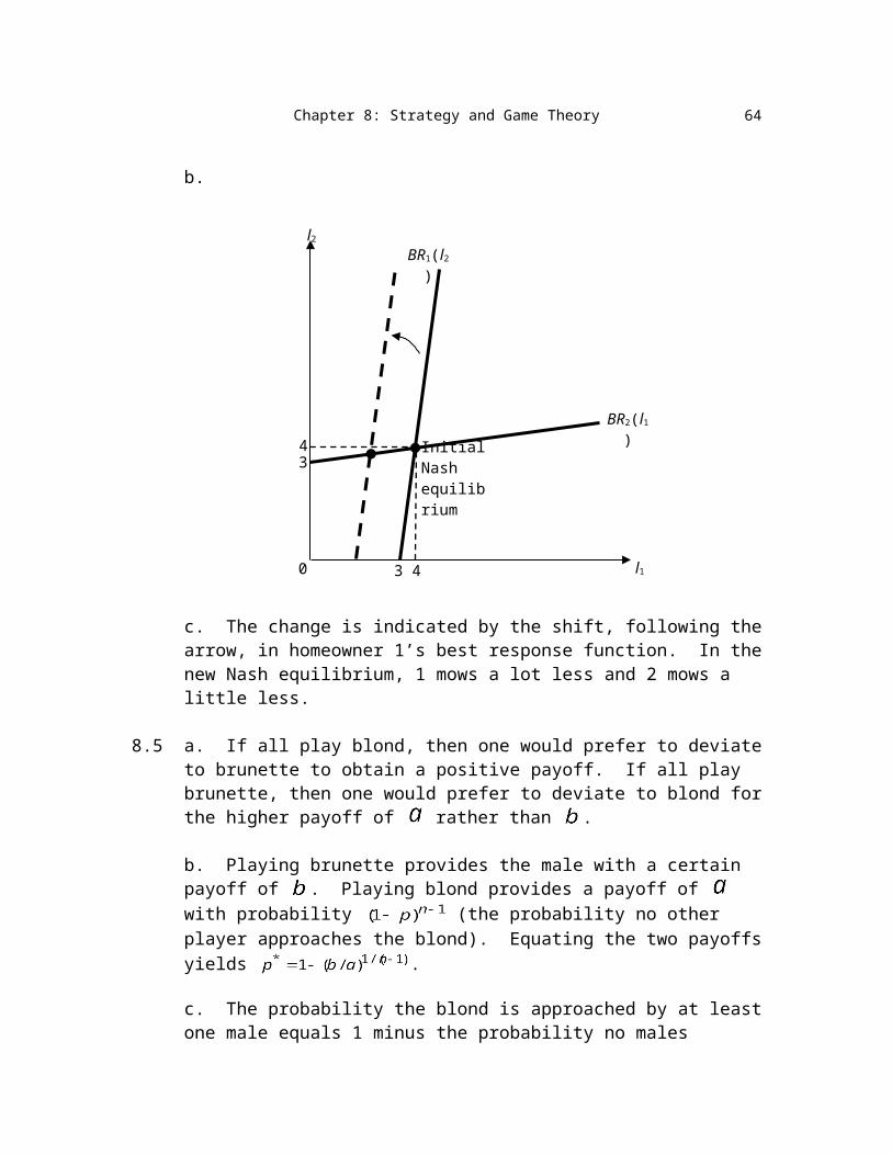
c. The change is indicated by the shift, following the arrow, in homeowner 1’s best response function. In the new Nash equilibrium, 1 mows a lot less and 2 mows a little less.

8.5 a. If all play blond, then one would prefer to deviate to brunette to obtain a positive payoff. If all play brunette, then one would prefer to deviate to blond for the higher payoff of rather than .

b. Playing brunette provides the male with a certain payoff of . Playing blond provides a payoff of with probability (the probability no other player approaches the blond). Equating the two payoffs yields .

c. The probability the blond is approached by at least one male equals 1 minus the probability no males approach her: . This expression is decreasing in because the exponent is decreasing in and the base of the exponent, , is a fraction.

8.6 a. Player 1’s minmax value is 0, achieved if 2 plays the pure strategy B. Player 2 can cause more harm to 1 by playing the mixed strategy of B with probability 9/10 and C with probability 1/10. Then 1’s highest expected payoff is -1/10.

0 3

3●

l1

l2

4

4

BR1(l2)

Initial Nashequilibrium

BR2(l1)

●

61


b. Each player can play the strategy of beginning with A in the first period. If no one deviated from A, C is played; otherwise B is played. Players earn a total of 18 each in equilibrium with these strategies (10 in the first period and 8 in the second). The strategies are subgame perfect. In the second period, a Nash equilibrium is always played, either (B, B) or (C, C). There is no incentive to deviate in the first period: the first-period gain from deviation of 5 is less than the second-period loss from moving to the less-preferred Nash equilibrium of 8.

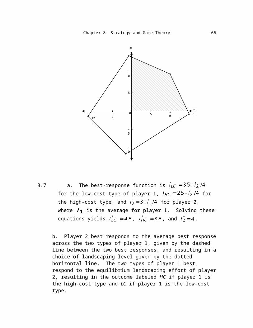
c. The outer polygon is the feasible set; payoffs in the shaded region are additionally above the minmax levels and thus are achievable in the limit.

8.7 a. The best-response function is for the low-cost type of player 1, for the high-cost type, and for player 2, where is

the average for player 1. Solving these equations yields , , and .

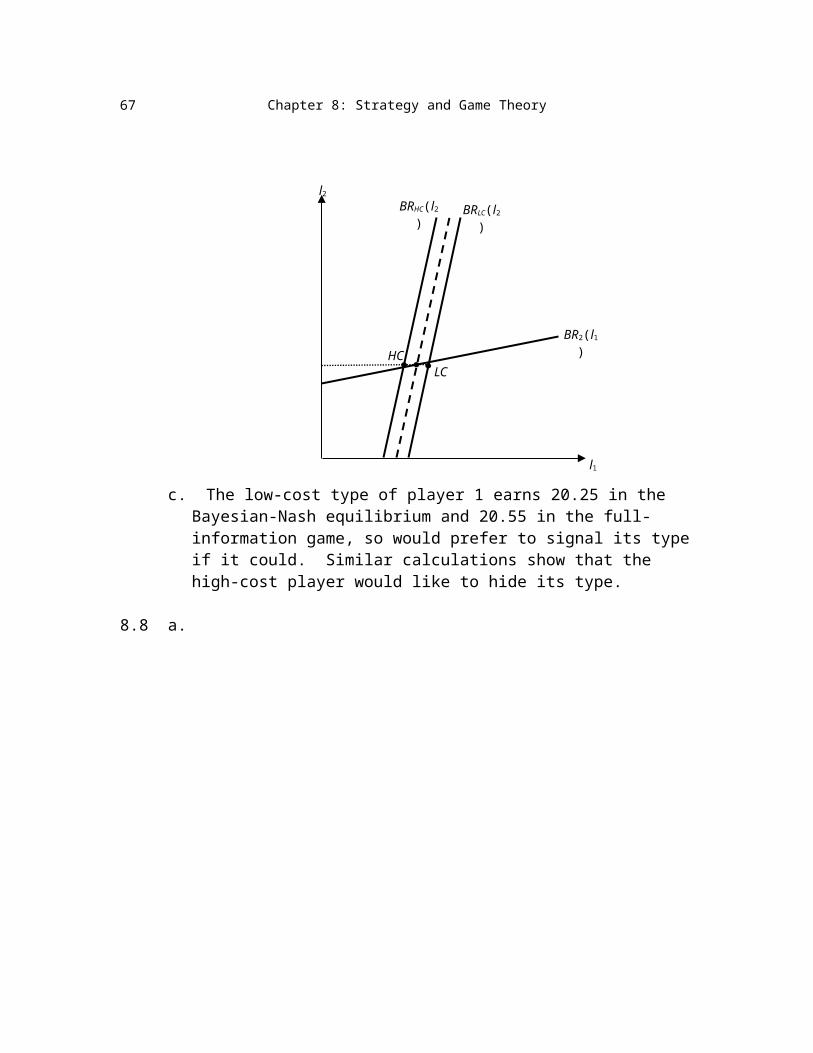
b. Player 2 best responds to the average best response across the two types of player 1, given by the dashed line between the two best responses, and resulting in a choice of landscaping level given by the dotted horizontal line. The two types of player 1 best respond to the equilibrium landscaping effort of player 2,

0 u15 10

-5-10

5

10

-5

-10

u2

62


resulting in the outcome labeled HC if player 1 is the high-cost type and LC if player 1 is the low-cost type.

c. The low-cost type of player 1 earns 20.25 in the Bayesian-Nash equilibrium and 20.55 in the full-information game, so would prefer to signal its type if it could. Similar calculations show that the high-cost player would like to hide its type.

8.8 a.

l1

l2

BRHC(l2)

BR2(l1)

BRLC(l2)

LCHC

63


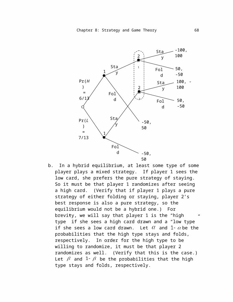
b. In a hybrid equilibrium, at least some type of some player plays a mixed strategy. If player 1 sees the low card, she prefers the pure strategy of staying. So it must be that player 1 randomizes after seeing a high card. (Verify that if player 1 plays a pure strategy of either folding or staying, player 2’s best response is also a pure strategy, so the equilibrium would not be a hybrid one.) For brevity, we will say that player 1 is the “high type” if she sees a high card drawn and a “low type” if she sees a low card drawn. Let and be the probabilities that the high type stays and folds, respectively. In order for the high type to be willing to randomize, it must be that player 2 randomizes as well. (Verify that this is the case.) Let and be the probabilities that the high type stays and folds, respectively.

must be such that the high type is indifferent between staying and folding for her to be willing to randomize. Staying provides the high type with an expected payoff of , and folding provides her with a payoff of -50. Equating these two expressions and solving yields .

In order for player 2 to be willing to randomize, he must be indifferent between staying and folding. His expected payoff from staying is

●1

Pr(H) = 6/13

Stay

Fold

●1

●2

●2

-50, 50

n1

n2

Fold

Stay

Pr(L)= 7/13

-50, 50

Stay

Stay

Fold

Fold

100, -100

50, -50

50, -50

-100, 100

64


where is the posterior probability that player 1 is the high type conditional on her staying. Player 2’s payoff from folding is -50. Equating the two expected payoffs yields . must also satisfy Bayes’ rule:

Equating this last expression with and solving yields .

To summarize, in the hybrid equilibrium, the low type always stays, the high type mixes between staying and folding with probabilities 7/18 and 11/18, and player 2 randomizes between staying and folding with probabilities 2/3 and 1/3. Player 2’s posterior beliefs are that player 1 is the high type with certainty if she folds; if she stays she is the high type with probability 1/4 and the low type with probability 3/4.

c. The low type’s expected payoff is (100)(2/3) + (50)(1/3) = 83.3. The high type’s expected payoff is -50 (she is indifferent between staying and folding in equilibrium, and earns -50 from folding). Given the prior probabilities of being a high and low type, player 1’s expected payoff from the game (prior to learning her type) is (83.3)(7/13) + (-50)(6/13) = 21.8. Player 2’s expected payoff is -50 (he is indifferent between staying and folding in equilibrium and earns -50 from folding). The game is clearly tilted toward player 1.

Analytical Problems:

8.9 Dominant strategies

For any strategy profile besides the dominant-strategy equilibrium, each player would have an incentive to deviate to its dominant strategy, ruling out the profile as a Nash equilibrium.

65


8.10 Rotten Kid Theorem

In the second stage, the parent chooses to maximize

yielding first-order condition

.

Even though the preceding equation cannot be solved explicitly for , we can still use the implicit function rule to find the derivative

.

In the first state, the child maximizes , yielding first-order condition

This equation implies , the first-order condition for maximizing their joint incomes.

8.11 Alternatives to Grim Strategy

a. Cooperating gives a stream of per-period payoffs of 2, for a present discounted value of . If players use tit-for-tat strategies, the present discounted value from deviating to fink at the start of the game is

66


.

The deviator earns 3 in the first period, followed by a period in which both fink and earn 1, followed by a return to cooperating in the third period and thereafter. For the displayed payoff not to exceed , , that is, players must be infinitely patient.

If players use two periods of punishment, the present discounted value from deviating is

.

For the displayed payoff not to exceed , we see, upon multiplying through by and simplifying, the required condition is . Factoring, . Hence, the required condition can be written . Using the quadratic formula to obtain the roots of this quadratic, we have .

b. The required condition is that the present discounted value of the payoffs from cooperating, , exceed that from deviating,

. Simplifying, . As the graph below shows, the expression crosses the x-axis very slightly to the left of 0.5. Using numerical methods or a more precise graph, it can be shown that the condition is . The resulting condition is very close to the condition for cooperation with infinitely many periods of punishment ( ).

67

-0.03

-0.02

-0.01

0

0.01

0.02

0.03

0.49 0.495 0.5 0.505 0.51


8.12 Refinements of perfect Bayesian equilibrium

a. The key condition is for the firm to be willing to offer a job to an uneducated worker. (Regarding the other player, the worker, all worker types obtain the highest payoffs possible, since they are hired and don’t have to expend the cost of education.) The firm’s expected payoff from J is

and from NJ is 0. The displayed expression exceeds 0 if . According to Bayes’ rule, along the equilibrium path, posterior beliefs are the same as prior beliefs in a pooling equilibrium. Therefore, . The required condition for the specified pooling equilibrium thus is .

All out-of-equilibrium beliefs and strategies are consistent with this pooling equilibrium. If , then the firm would choose J conditional on observing E. On the other hand, if , then the firm would choose NJ conditional on observing E.

b. For the firm to prefer not to offer a job to an uneducated worker, calculations similar to those in part (a) (but with the inequalities reversed) imply

. A high skilled worker would deviate to E unless the firm chooses NJ conditional on E. The firm prefers NJ to J conditional on E when the out-of-equilibrium posterior beliefs satisfy or equivalently . Suppose . Then it would be unreasonable to think that type L would ever deviate to E. Regardless of what strategy the firm plays, type L’s payoff would be negative from E and non-negative from NE. (By contrast, type H may have an incentive to deviate: he or she earns a positive payoff if the firm plays J conditional on E.) The Cho-Kreps intuitive criterion restricts the out-of-equilibrium posterior belief

. Since is inconsistent with the required condition , the Cho-Kreps intuitive criterion rules out the pooling

equilibrium specified in part (b), leaving only the one specified in part (a).

68

MT10 Ch8 solns

Documents

Transcript of MT10 Ch8 solns