MRI for

Radiation Therapy Planning

(2)

Yue Cao, Ph.D.

Departments of Radiation Oncology, Radiology and Biomedical Engineering

University of Michigan

Panel: J. Balter, E. Paulson, R Cormack

2

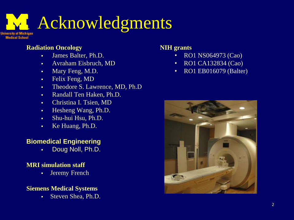
Acknowledgments

Radiation Oncology

James Balter, Ph.D.

Avraham Eisbruch, MD

Mary Feng, M.D.

Felix Feng, MD

Theodore S. Lawrence, MD, Ph.D

Randall Ten Haken, Ph.D.

Christina I. Tsien, MD

Hesheng Wang, Ph.D.

Shu-hui Hsu, Ph.D.

Ke Huang, Ph.D.

Biomedical Engineering

Doug Noll, Ph.D.

MRI simulation staff

Jeremy French

Siemens Medical Systems

Steven Shea, Ph.D.

NIH grants

• RO1 NS064973 (Cao)

• RO1 CA132834 (Cao)

• RO1 EB016079 (Balter)

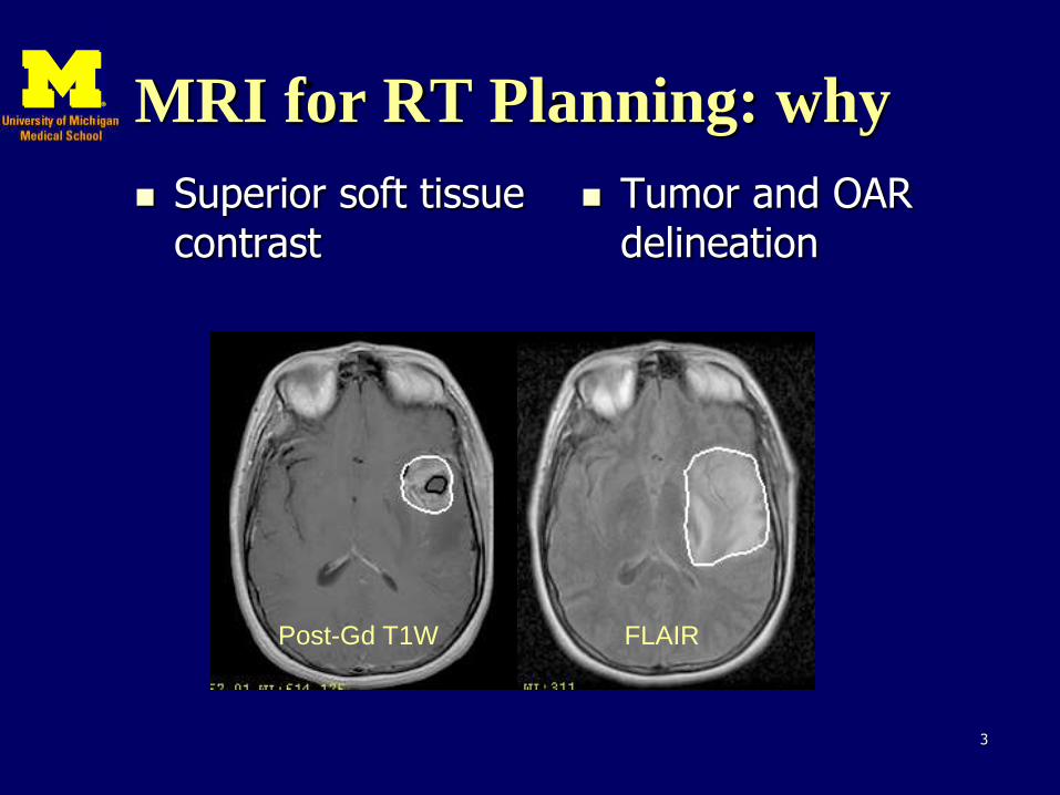
MRI for RT Planning: why

Superior soft tissue contrast

Tumor and OAR delineation

3

Post-Gd T1W FLAIR

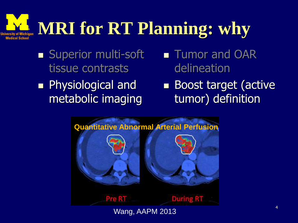
MRI for RT Planning: why

Superior multi-soft tissue contrasts

Physiological and metabolic imaging

Tumor and OAR delineation

Boost target (active tumor) definition

4

Quantitative Abnormal Arterial Perfusion

Wang, AAPM 2013

Integration of MRI in RT

Target and/or Boost volume definition

OAR delineation and organ function assessment

Treatment Planning

Motion management

On-board Tx verification

Early Tx response assessment

– to image active residual tumor

– to assess normal tissue/organ function reserve 5

MRI Simulator

MRI scanner is designed for diagnosis

Challenges for use as a RT simulator:

– System-level geometric accuracy

– Patient-induced spatial distortion

– Electron density (synthetic CT)

– IGRT support

– RF coil configuration optimization

– Sequence optimization for RT planning

– Etc. 6

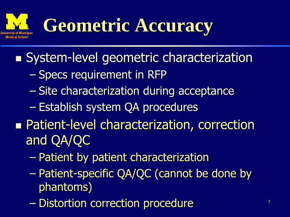
Geometric Accuracy

System-level geometric characterization

– Specs requirement in RFP

– Site characterization during acceptance

– Establish system QA procedures

Patient-level characterization, correction and QA/QC

– Patient by patient characterization

– Patient-specific QA/QC (cannot be done by phantoms)

– Distortion correction procedure

7

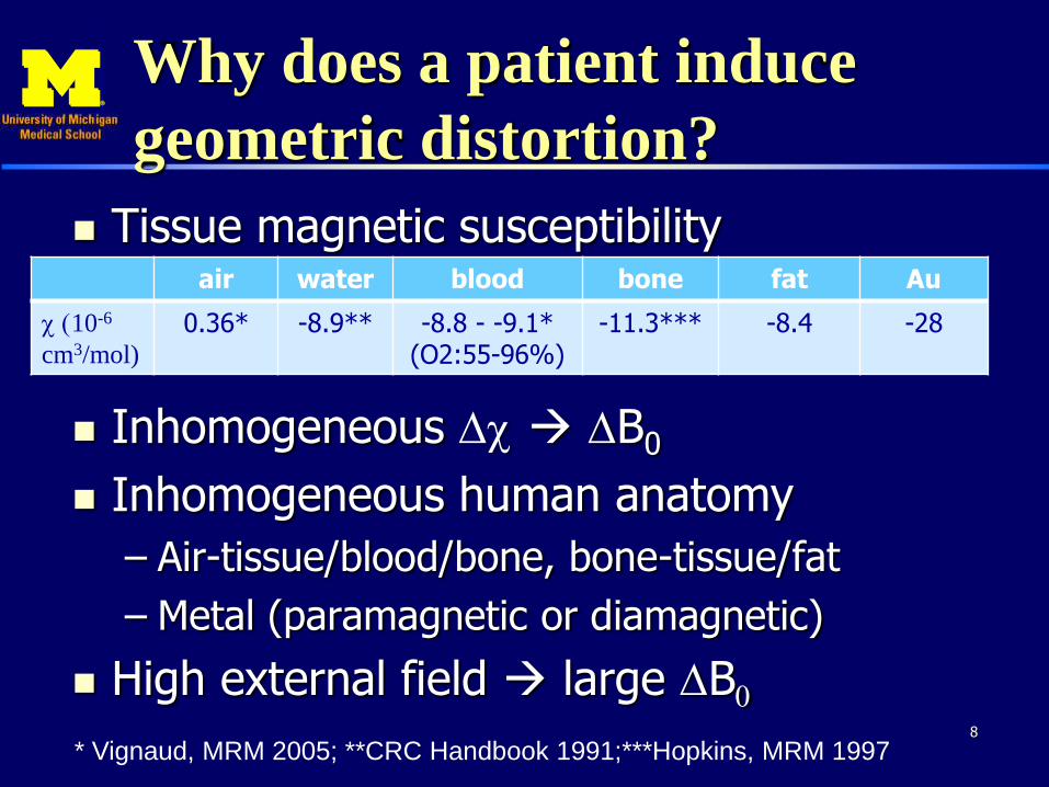
Why does a patient induce

geometric distortion?

Tissue magnetic susceptibility

Inhomogeneous Dc DB0

Inhomogeneous human anatomy

– Air-tissue/blood/bone, bone-tissue/fat

– Metal (paramagnetic or diamagnetic)

High external field large DB0

8

air water blood bone fat Au

c (10-6

cm3/mol)

0.36* -8.9** -8.8 - -9.1* (O2:55-96%)

-11.3*** -8.4 -28

* Vignaud, MRM 2005; **CRC Handbook 1991;***Hopkins, MRM 1997

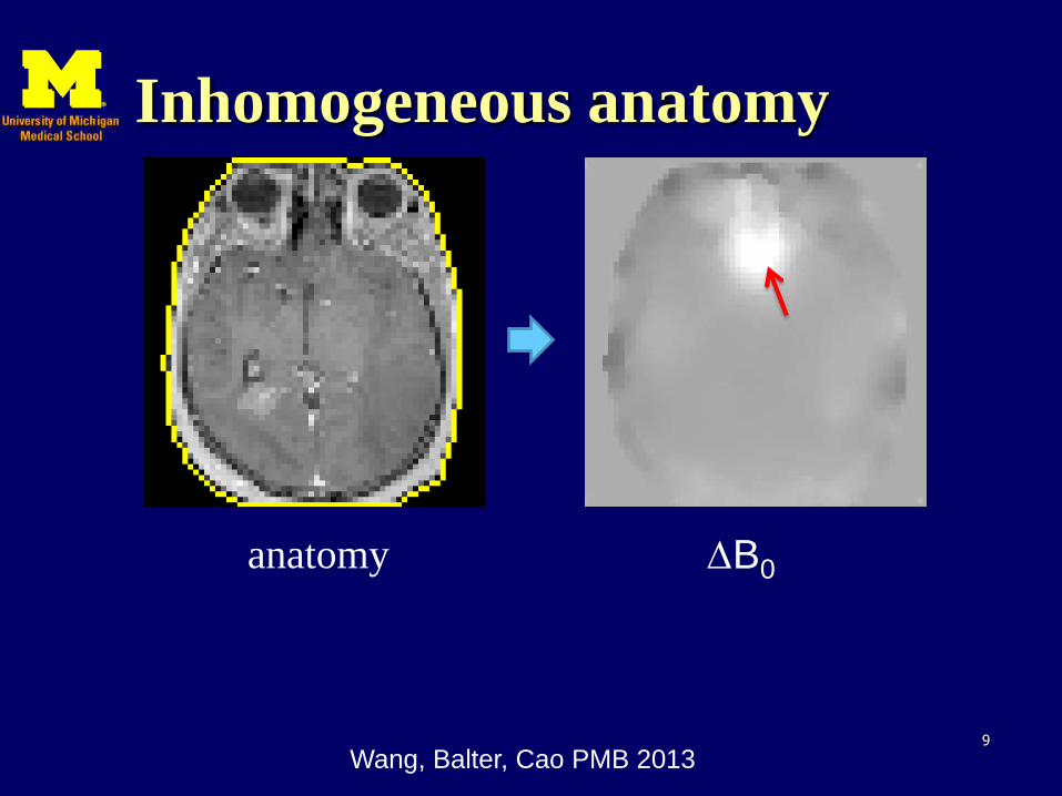
Inhomogeneous anatomy

9

DB0 anatomy

Wang, Balter, Cao PMB 2013

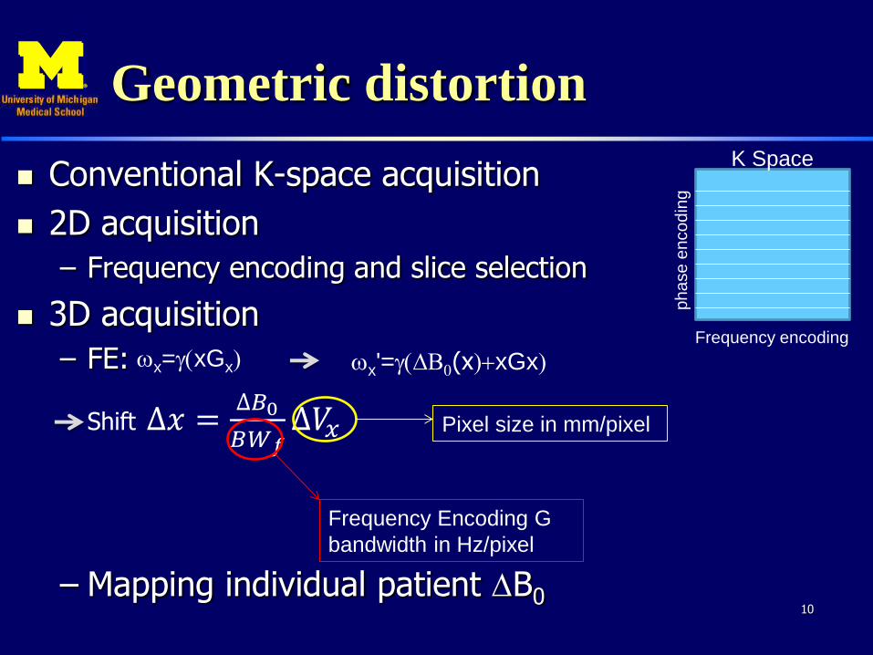
Geometric distortion

Conventional K-space acquisition

2D acquisition

– Frequency encoding and slice selection

3D acquisition

– FE:

– Shift ∆𝑥 =∆𝐵0

𝐵𝑊𝑓∆𝑉𝑥

– Mapping individual patient DB0 10

Frequency Encoding G

bandwidth in Hz/pixel

Pixel size in mm/pixel

wx=g(xGx)

K Space

Frequency encoding

ph

ase

en

co

din

g

wx'=g(DB0(x)+xGx)

Patient-level Distortion

Correction and QA

11

Acquire wrapped

phase different maps

by 2 gradient

echoes

Unwrap and

convert to

the field map

Correct gradient non-

linearity

Assess whether a

distortion correction

is needed for images

Correct distortion

Or stop

-4

-2

0

2

4

6

8

10

12

0 2 4 6 8

fie

ld (

pp

m o

r H

z)

X (mm)-4

-3

-2

-1

0

1

2

3

4

0 2 4 6 8

Ph

ase

(ra

dia

n)

X (mm)

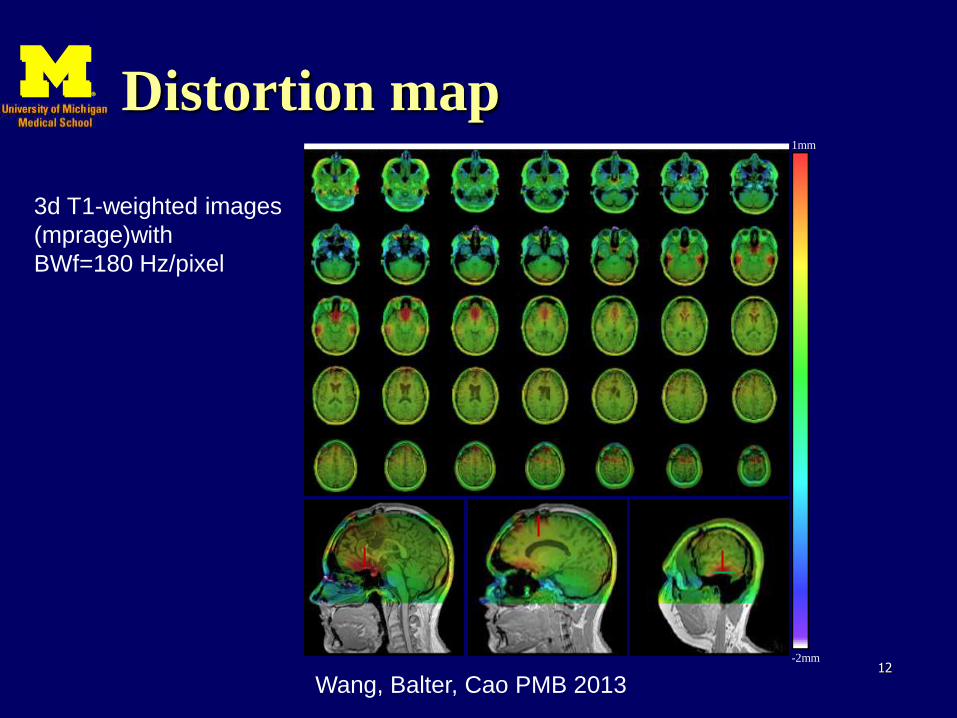
Distortion map

12

1mm

-2mm

Wang, Balter, Cao PMB 2013

3d T1-weighted images

(mprage)with

BWf=180 Hz/pixel

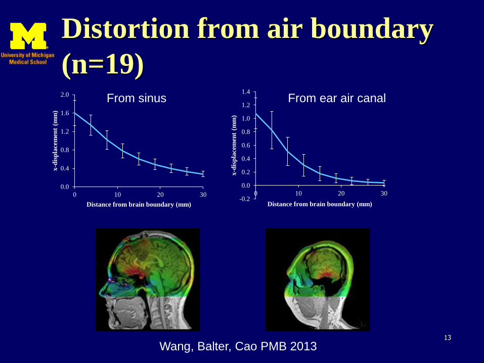
Distortion from air boundary

(n=19)

13

0.0

0.4

0.8

1.2

1.6

2.0

0 10 20 30

x-d

isp

lace

men

t (m

m)

Distance from brain boundary (mm) -0.2

0.0

0.2

0.4

0.6

0.8

1.0

1.2

1.4

0 10 20 30

x-d

isp

lace

men

t (m

m)

Distance from brain boundary (mm)

From sinus From ear air canal

Wang, Balter, Cao PMB 2013

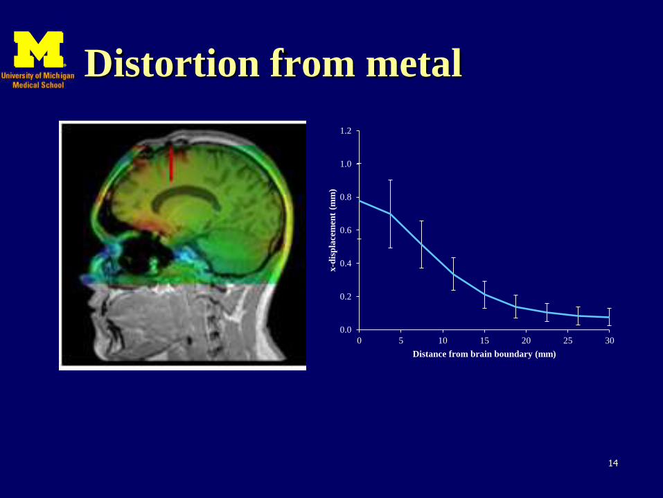
Distortion from metal

14

0.0

0.2

0.4

0.6

0.8

1.0

1.2

0 5 10 15 20 25 30x-d

isp

lace

men

t (m

m)

Distance from brain boundary (mm)

Perturbation in DB0 map due

to object movement

Uniform water phantom

• DB0 map (0 min) vs DB0 map (15 min) after moving a water phantom into the scanner bore

Human subject

• Does DB0 map change over scanning time?

• If yes, what does it impact on geometric accuracy of the images?

15

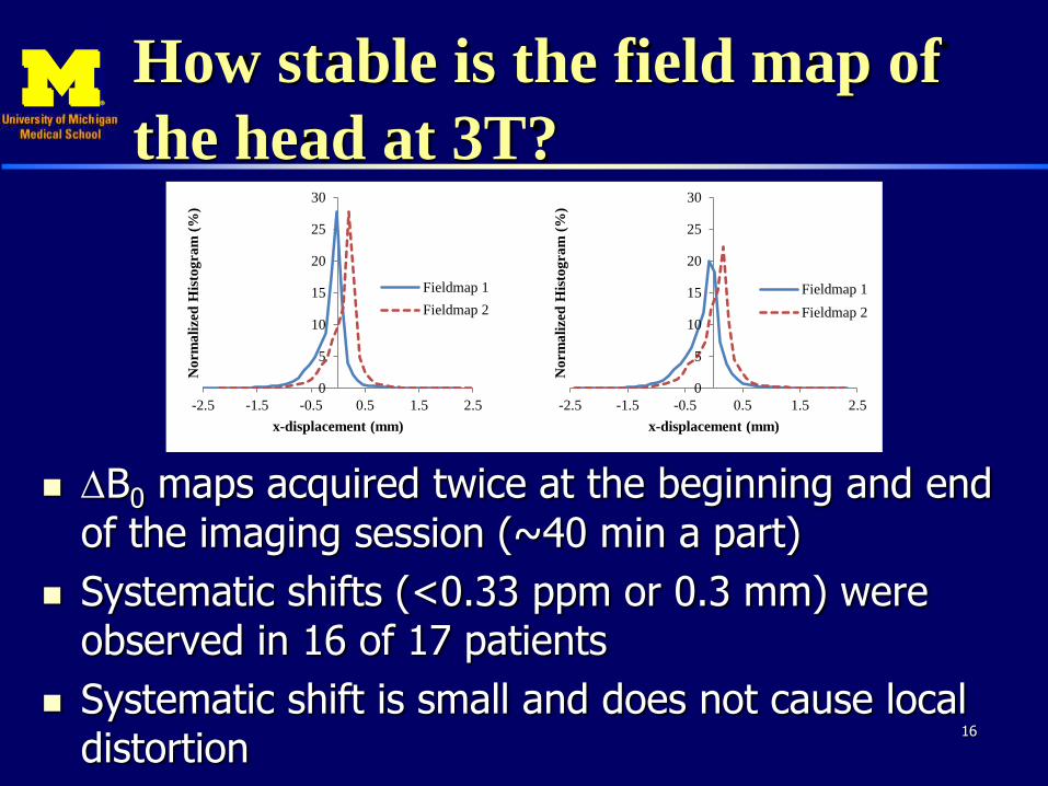
How stable is the field map of

the head at 3T?

DB0 maps acquired twice at the beginning and end of the imaging session (~40 min a part)

Systematic shifts (<0.33 ppm or 0.3 mm) were observed in 16 of 17 patients

Systematic shift is small and does not cause local distortion

16

0

5

10

15

20

25

30

-2.5 -1.5 -0.5 0.5 1.5 2.5

No

rma

lize

d H

isto

gra

m (

%)

x-displacement (mm)

Fieldmap 1

Fieldmap 2

0

5

10

15

20

25

30

-2.5 -1.5 -0.5 0.5 1.5 2.5

No

rma

lize

d H

isto

gra

m (

%)

x-displacement (mm)

Fieldmap 1

Fieldmap 2

Chemical Shift: water and fat

Difference between resonance frequencies of water and fat

– 3.5 ppm

– 1.5T: 224 Hz; 3T: 448 Hz

Mismapping in frequency encoding and slice selection directions

At 3T,

if BWf=200Hx/1mm 2.24 mm

if BWf=800Hx/1mm 0.56 mm

17

Spin echo sequence

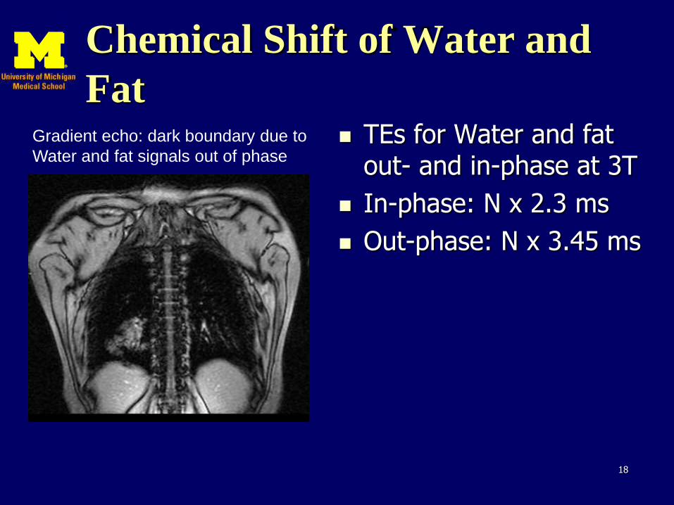
Chemical Shift of Water and

Fat TEs for Water and fat

out- and in-phase at 3T

In-phase: N x 2.3 ms

Out-phase: N x 3.45 ms

18

Gradient echo: dark boundary due to

Water and fat signals out of phase

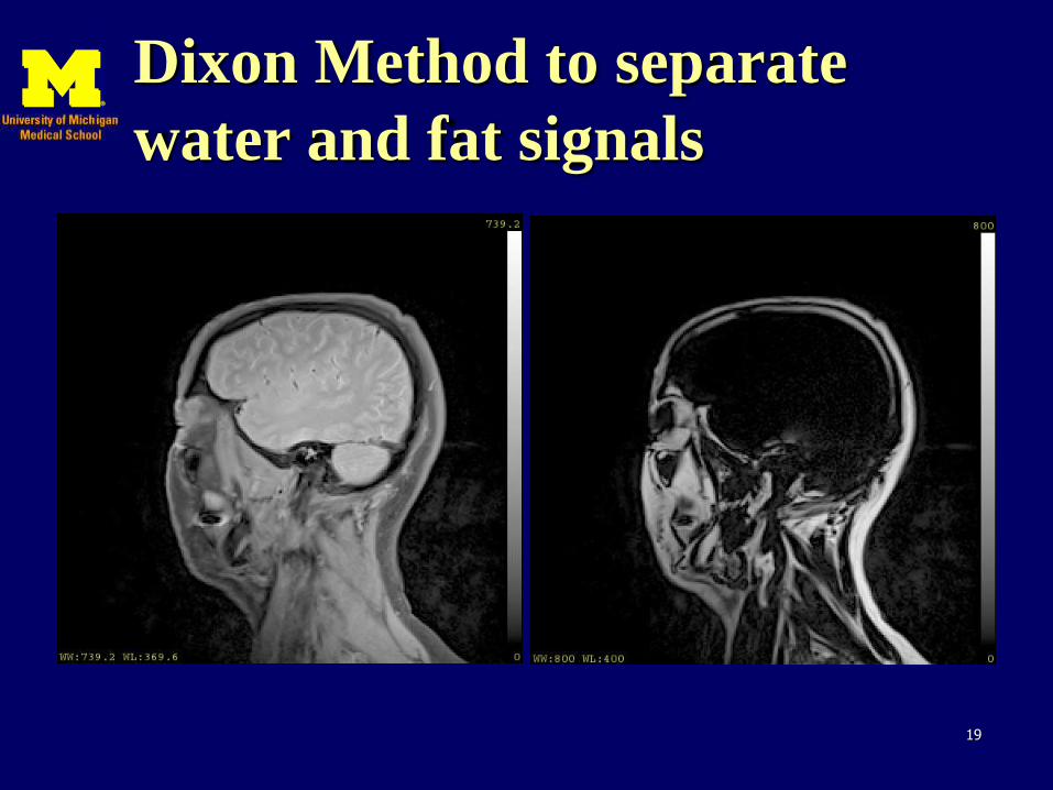
Dixon Method to separate

water and fat signals

19

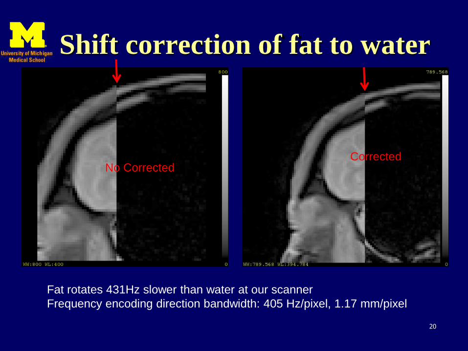
Shift correction of fat to water

20

No Corrected Corrected

Fat rotates 431Hz slower than water at our scanner

Frequency encoding direction bandwidth: 405 Hz/pixel, 1.17 mm/pixel

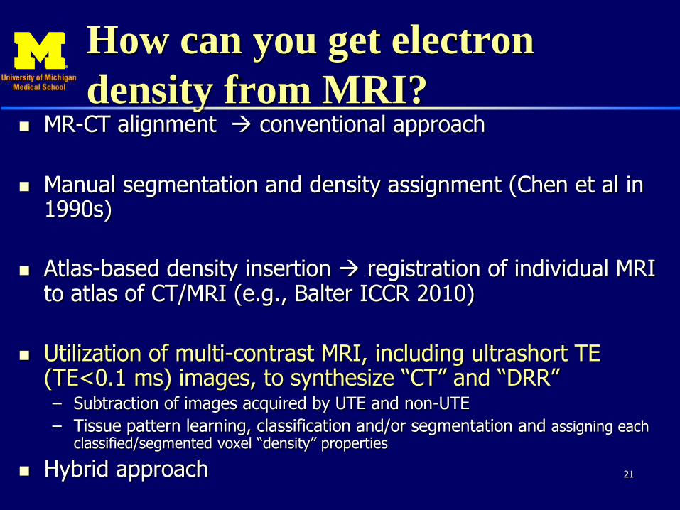
How can you get electron

density from MRI? MR-CT alignment conventional approach

Manual segmentation and density assignment (Chen et al in 1990s)

Atlas-based density insertion registration of individual MRI to atlas of CT/MRI (e.g., Balter ICCR 2010)

Utilization of multi-contrast MRI, including ultrashort TE (TE<0.1 ms) images, to synthesize “CT” and “DRR” – Subtraction of images acquired by UTE and non-UTE

– Tissue pattern learning, classification and/or segmentation and assigning each classified/segmented voxel “density” properties

Hybrid approach

21

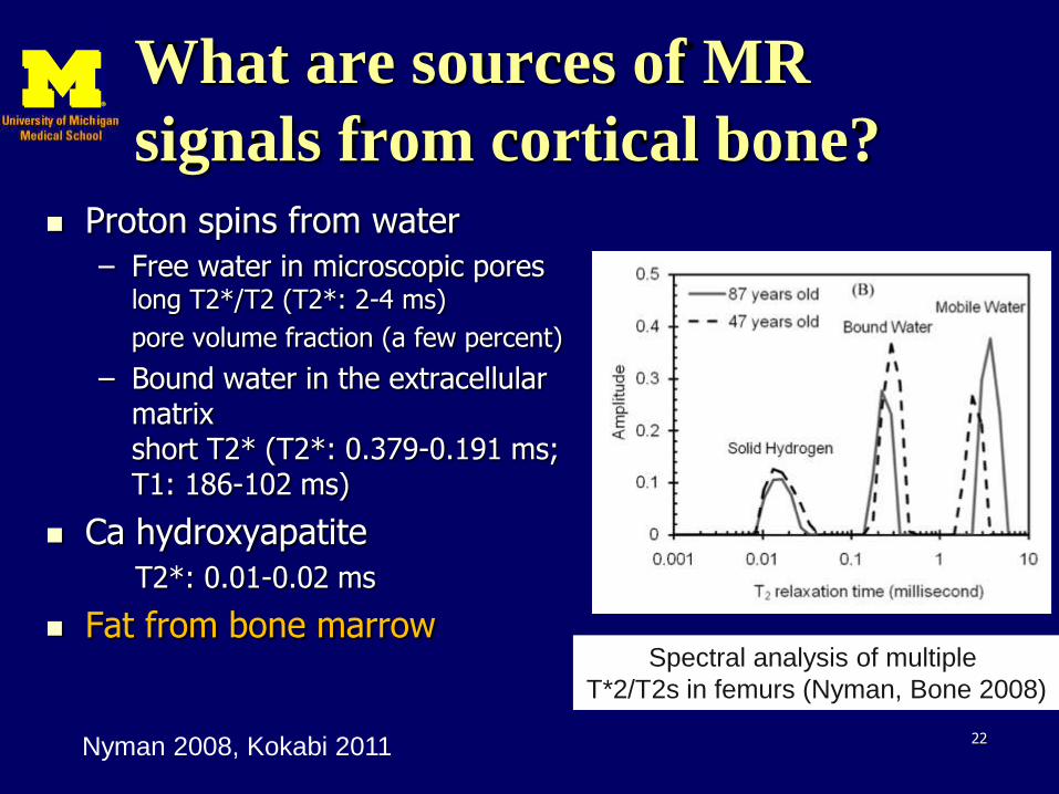
What are sources of MR

signals from cortical bone? Proton spins from water

– Free water in microscopic pores long T2*/T2 (T2*: 2-4 ms)

pore volume fraction (a few percent)

– Bound water in the extracellular matrix short T2* (T2*: 0.379-0.191 ms; T1: 186-102 ms)

Ca hydroxyapatite

T2*: 0.01-0.02 ms

Fat from bone marrow

22 Nyman 2008, Kokabi 2011

Spectral analysis of multiple

T*2/T2s in femurs (Nyman, Bone 2008)

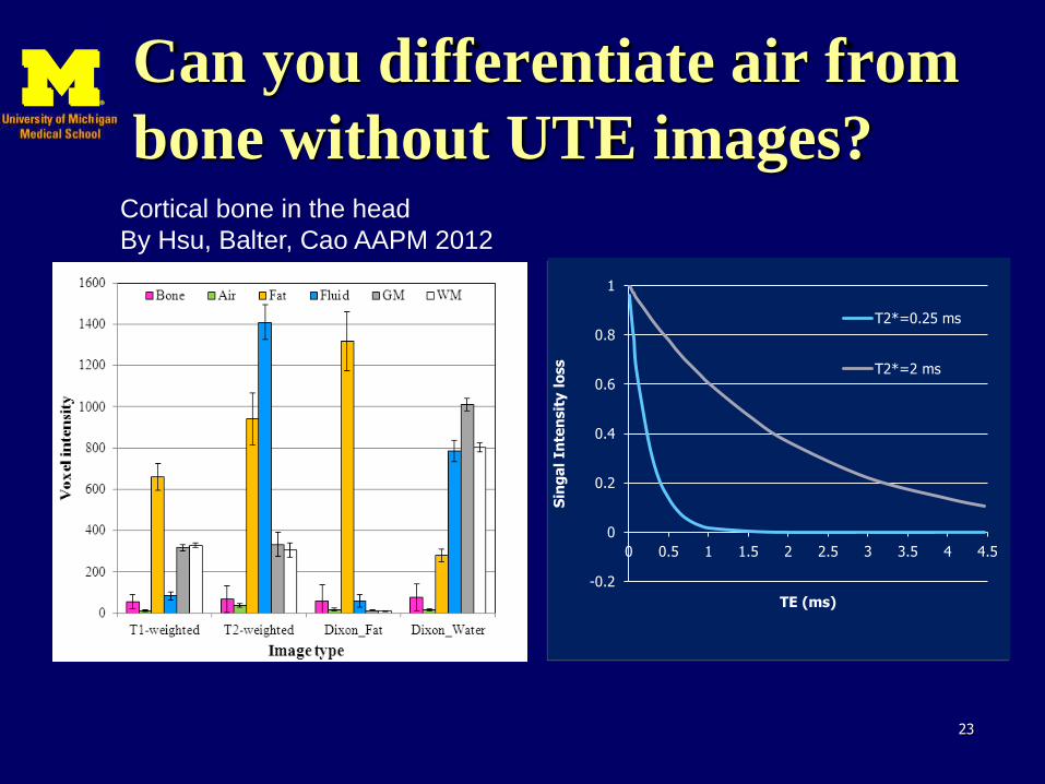
Can you differentiate air from

bone without UTE images?

23

Cortical bone in the head

By Hsu, Balter, Cao AAPM 2012

0

0.2

0.4

0.6

0.8

1

0 0.2 0.4 0.6 0.8 1 1.2 1.4 1.6 1.8 2Si

nga

l In

ten

sity

loss

TE (ms)

T2*=0.25 ms

0.45

0.05

0.018 Conventional TE

UTE

-0.2

0

0.2

0.4

0.6

0.8

1

0 0.5 1 1.5 2 2.5 3 3.5 4 4.5S

ing

al

Inte

nsit

y l

oss

TE (ms)

T2*=0.25 ms

T2*=2 ms

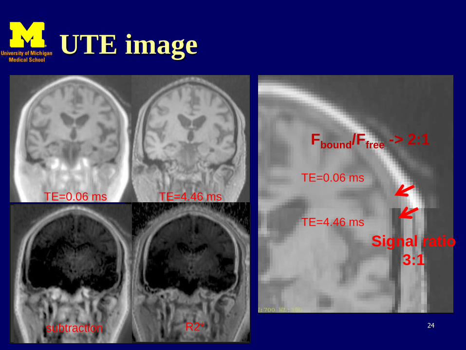
UTE image

24

TE=0.06 ms TE=4.46 ms

subtraction R2*

TE=4.46 ms

TE=0.06 ms

Signal ratio

3:1

Fbound/Ffree -> 2:1

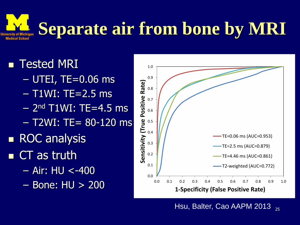
Separate air from bone by MRI

Tested MRI

– UTEI, TE=0.06 ms

– T1WI: TE=2.5 ms

– 2nd T1WI: TE=4.5 ms

– T2WI: TE= 80-120 ms

ROC analysis

CT as truth

– Air: HU <-400

– Bone: HU > 200

25 Hsu, Balter, Cao AAPM 2013

0.0

0.1

0.2

0.3

0.4

0.5

0.6

0.7

0.8

0.9

1.0

0.0 0.1 0.2 0.3 0.4 0.5 0.6 0.7 0.8 0.9 1.0

Sen

siti

vity

(Tr

ue

Po

siti

ve R

ate

)

1-Specificity (False Positive Rate)

TE=0.06 ms (AUC=0.953)

TE=2.5 ms (AUC=0.879)

TE=4.46 ms (AUC=0.861)

T2-weighted (AUC=0.772)

Synthetic CT:

Multispectral modeling

MRI signals provide various sources of contrast

By combining the information from multiple scans of the same tissue, we classify different tissue types

Assigning properties to these classified tissues permits generation of attenuation maps, as well as synthetic CT scans

26

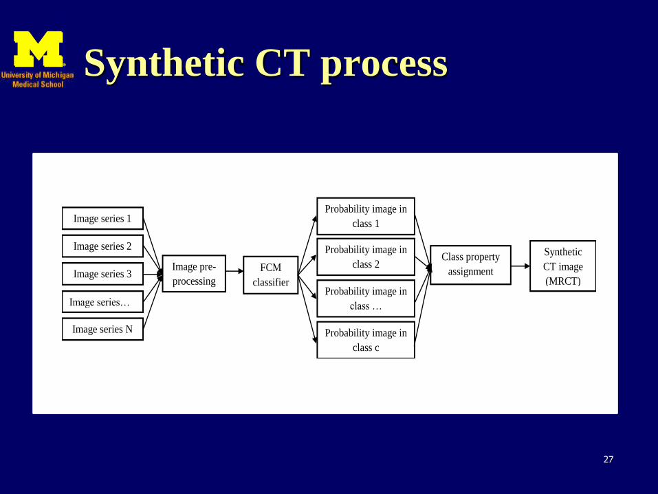
Synthetic CT process

27

Image series 1

Image series 2

Image series 3

Image series…

Image series N

FCM

classifier

Probability image in

class 1

Probability image in

class 2

Probability image in

class …

Probability image in

class c

Class property

assignment

Synthetic

CT image

(MRCT)

Image pre-

processing

UM protocol and coil setup

3T Skyra

Protocol

– Localizer

– TOF white vessel

– T1W-MPRAGE

– UTE (TE=0.06 ms)

– T2W-SPACE

– Dixon (fat and water)

– Total time 12.5 min

Coils

– Body18 + large flexible coil

indexed flat table top insert

Patient in Tx position and w mask

28

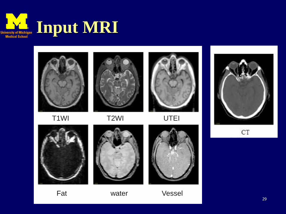
Input MRI

29

T1WI T2WI UTEI

Fat water Vessel

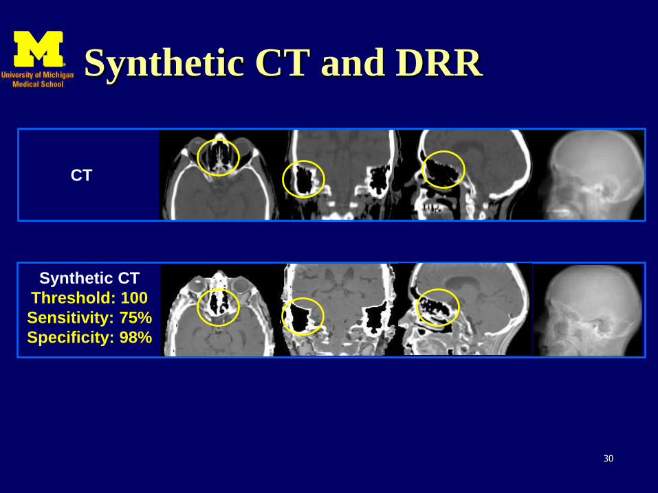
Synthetic CT and DRR

30

CT

Synthetic CT

Threshold: 100

Sensitivity: 75%

Specificity: 98%

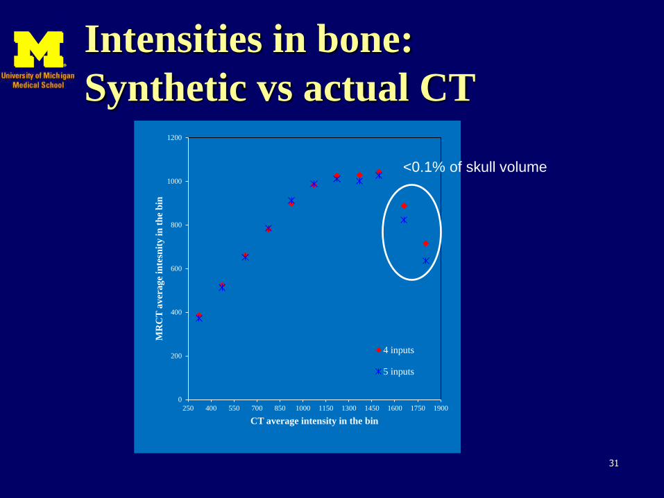
Intensities in bone:

Synthetic vs actual CT

31

0

200

400

600

800

1000

1200

250 400 550 700 850 1000 1150 1300 1450 1600 1750 1900

MR

CT

aver

age

inte

snit

y i

n t

he

bin

CT average intensity in the bin

4 inputs

5 inputs

<0.1% of skull volume

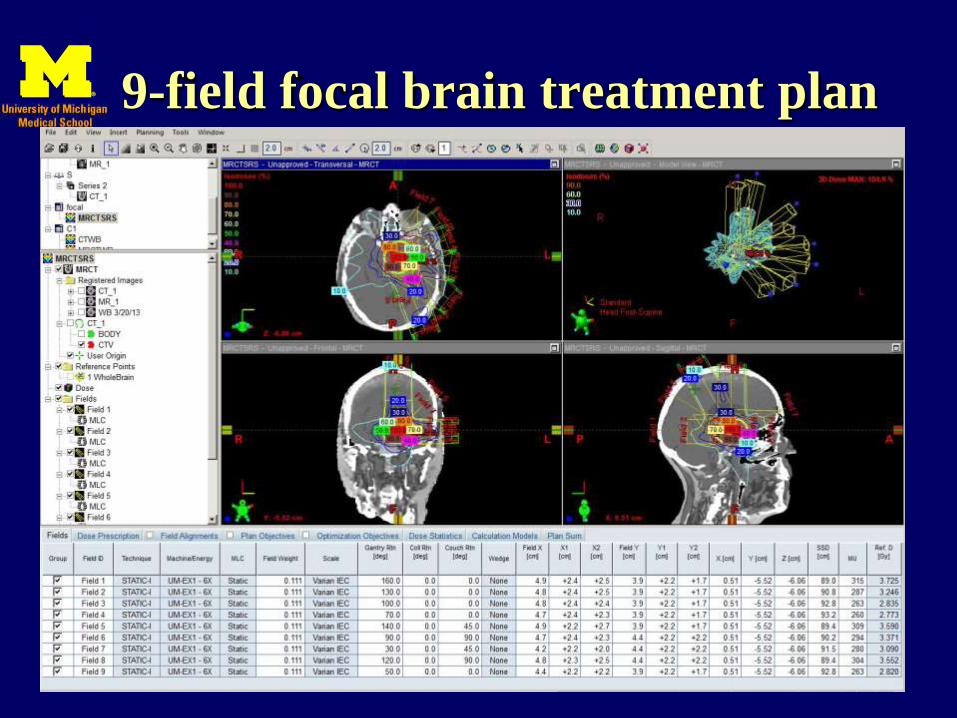
9-field focal brain treatment plan

32

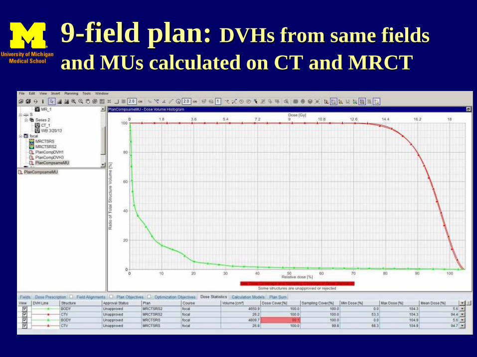
9-field plan: DVHs from same fields

and MUs calculated on CT and MRCT

33

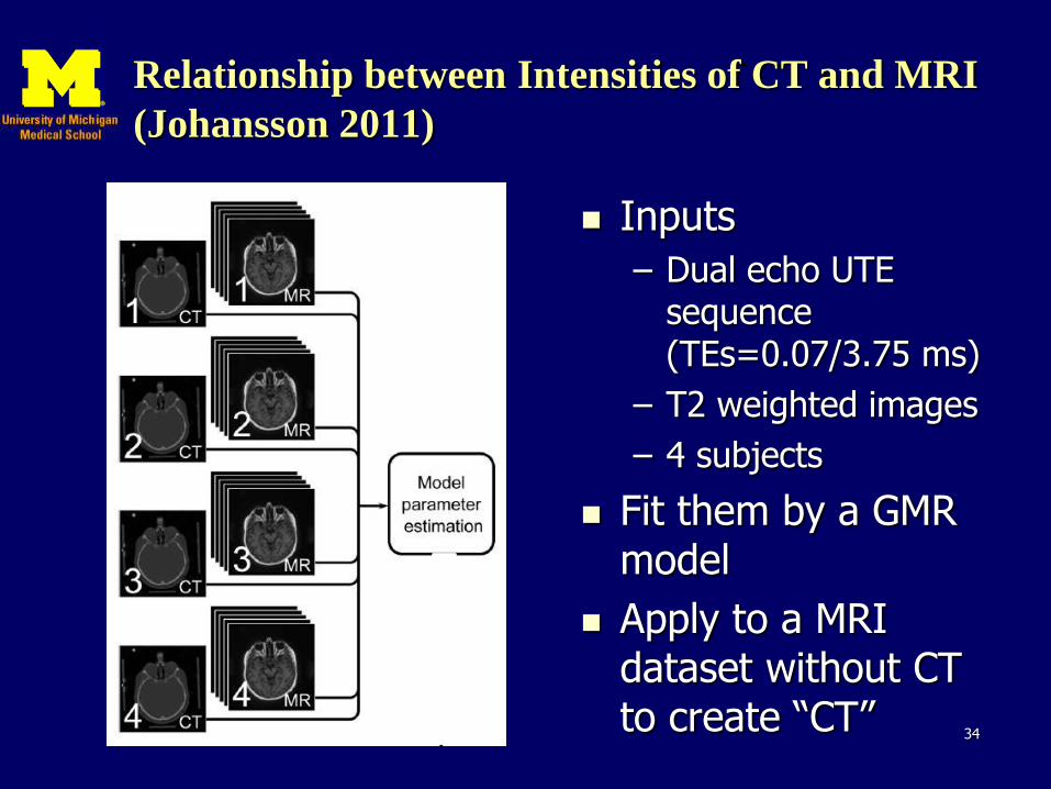
Relationship between Intensities of CT and MRI

(Johansson 2011)

Inputs

– Dual echo UTE sequence (TEs=0.07/3.75 ms)

– T2 weighted images

– 4 subjects

Fit them by a GMR model

Apply to a MRI dataset without CT to create “CT”

34

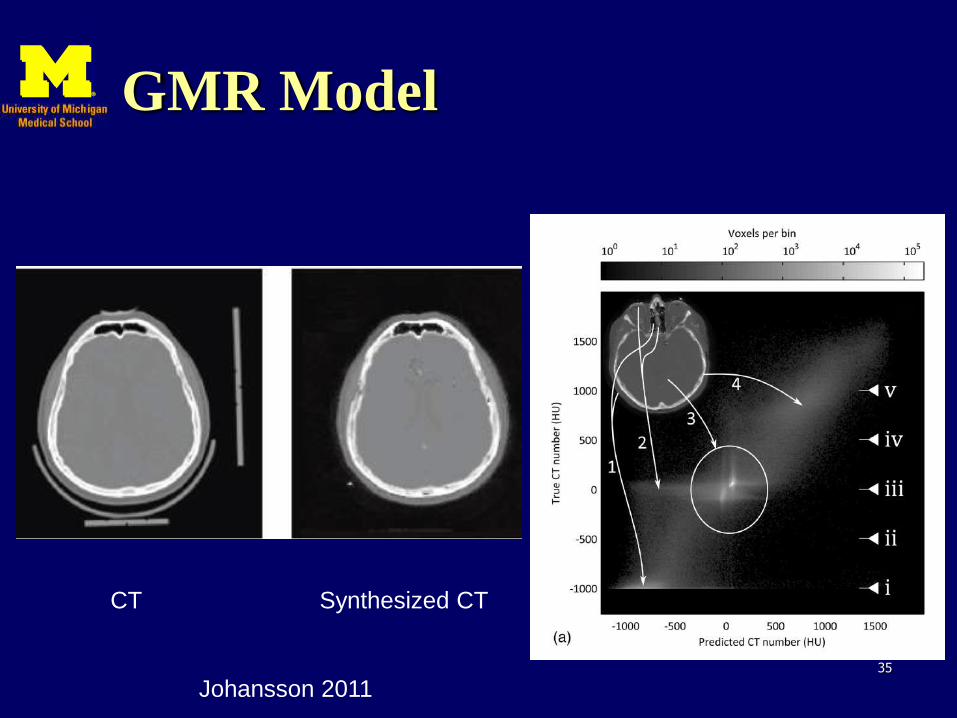
GMR Model

35

CT Synthesized CT

Johansson 2011

How to evaluate synthesized

“CT” or “DRR”

Voxel-to-voxel comparison of intensities between “CT” and CT (or “DRR” to DRR

Considering attempted uses

– Radiation dose plans created from “CT” vs CT

– Image guidance consequences using “DRR” vs DRR

Other criteria?

36

Challenges outside of head

Organ motion

Presence of other materials

– Iron, large fat fractions, cartilage,…

Large B1 field inhomogeneity

Variable air pockets

UTE sequence

37

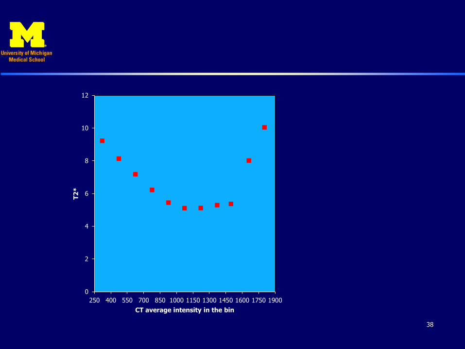
38

0

2

4

6

8

10

12

250 400 550 700 850 1000 1150 1300 1450 1600 1750 1900

T2

*

CT average intensity in the bin

Geometric phantom:

System level characterization

39

X: 29 Columns; Y: 21 rows; Z: 9 Sheets

Center to center 16 mm

Z

y

x

y x

y

z

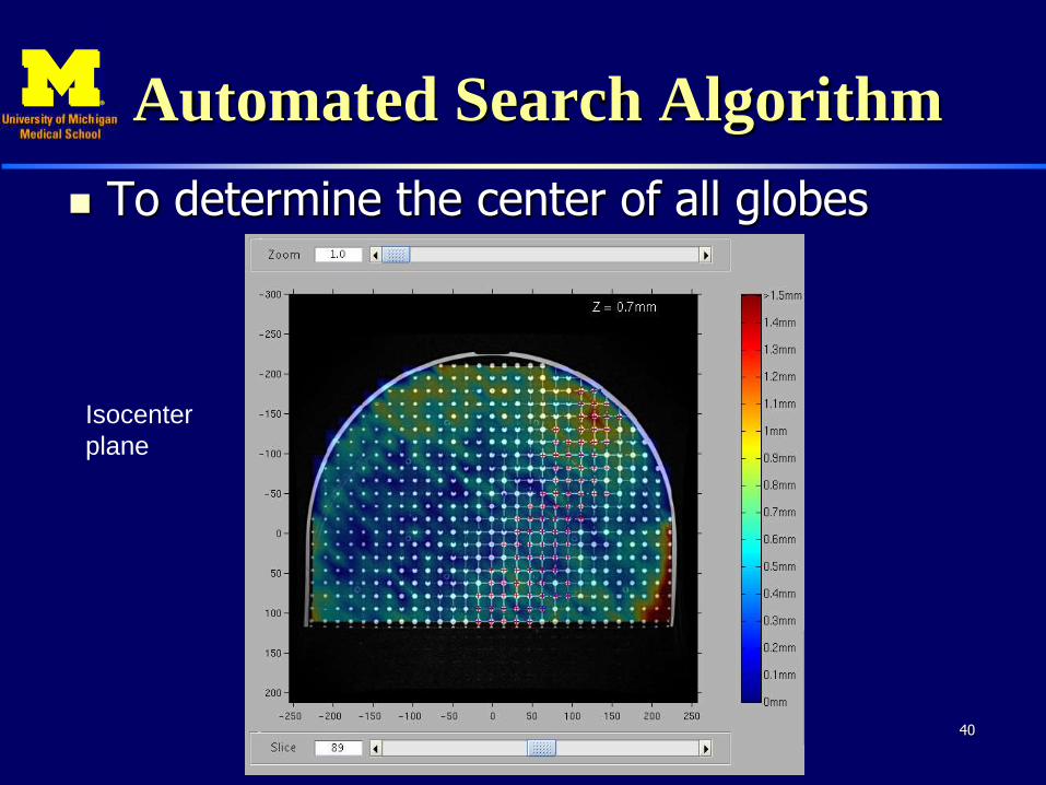
Automated Search Algorithm

To determine the center of all globes

40

Isocenter

plane

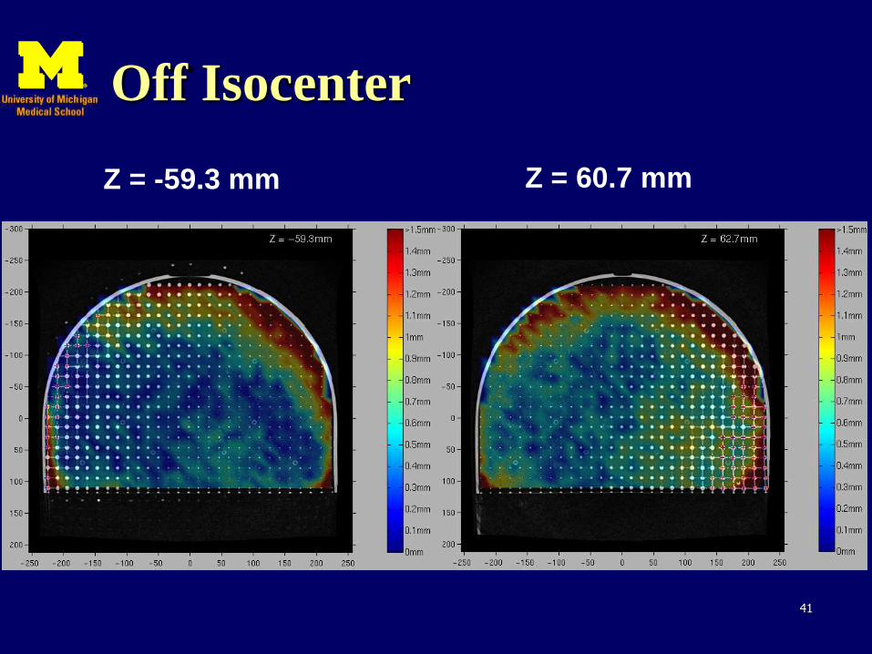
Off Isocenter

41

Z = -59.3 mm Z = 60.7 mm

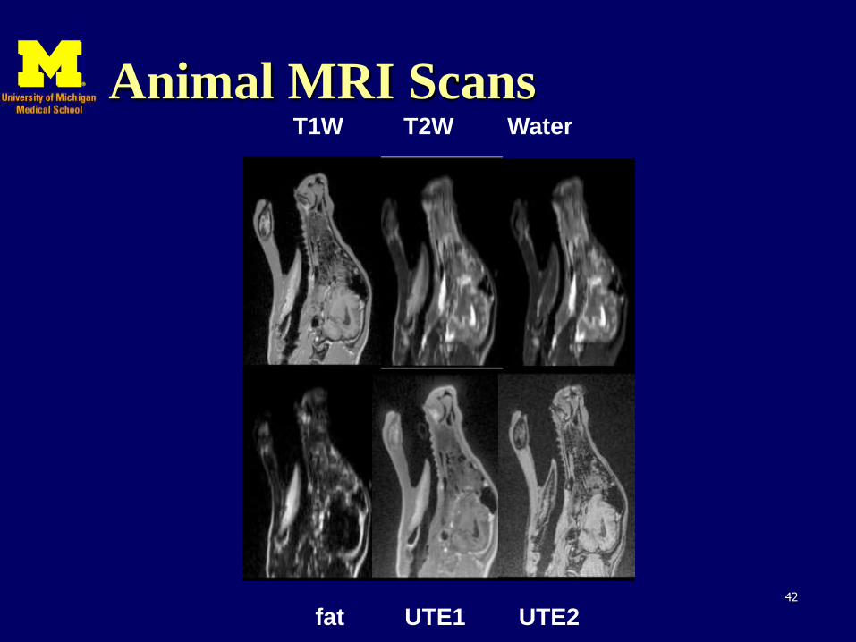
Animal MRI Scans

42

T1W T2W Water

fat UTE1 UTE2

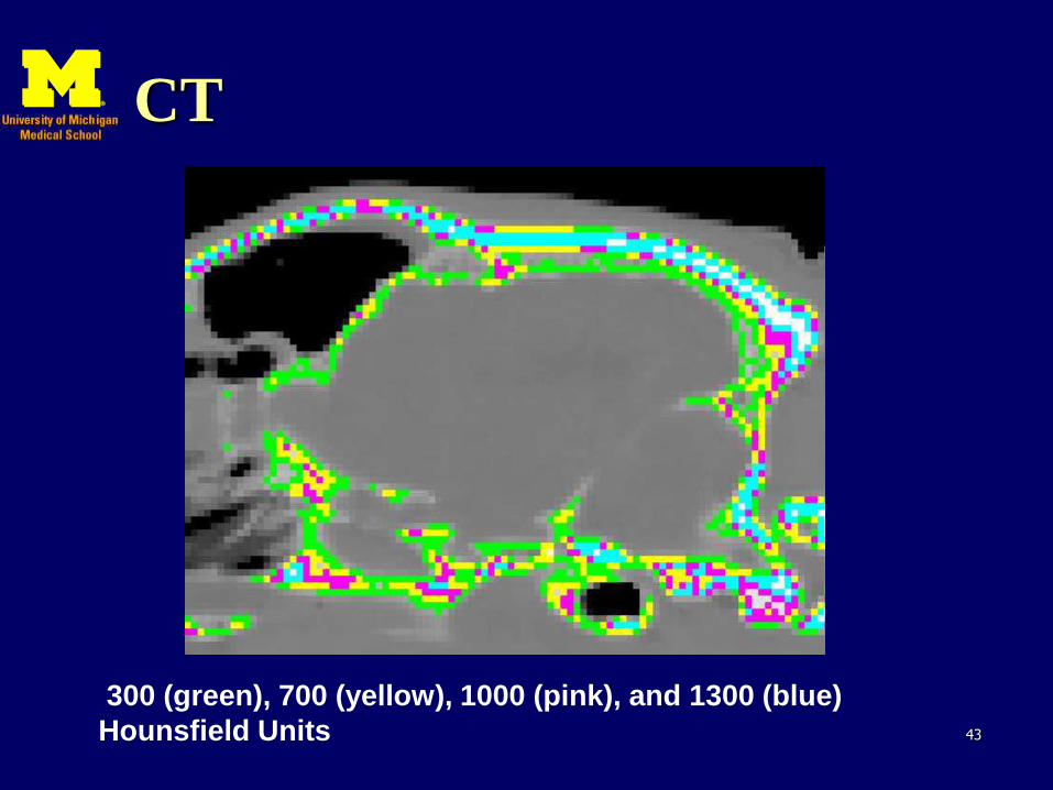
CT

43

300 (green), 700 (yellow), 1000 (pink), and 1300 (blue)

Hounsfield Units

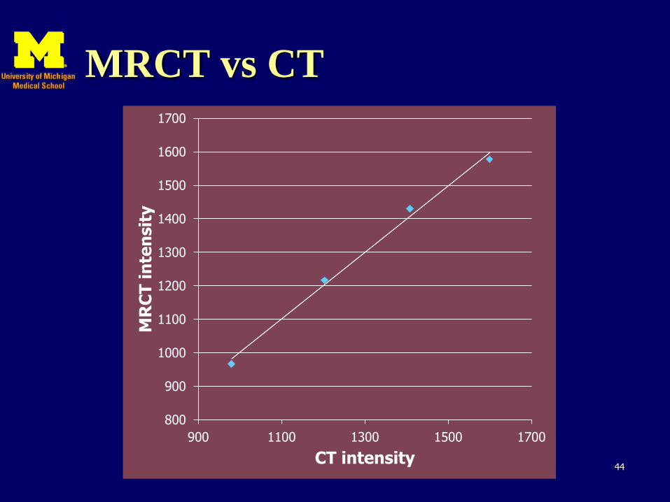
MRCT vs CT

44

800

900

1000

1100

1200

1300

1400

1500

1600

1700

900 1100 1300 1500 1700

MR

CT

in

ten

sit

y

CT intensity

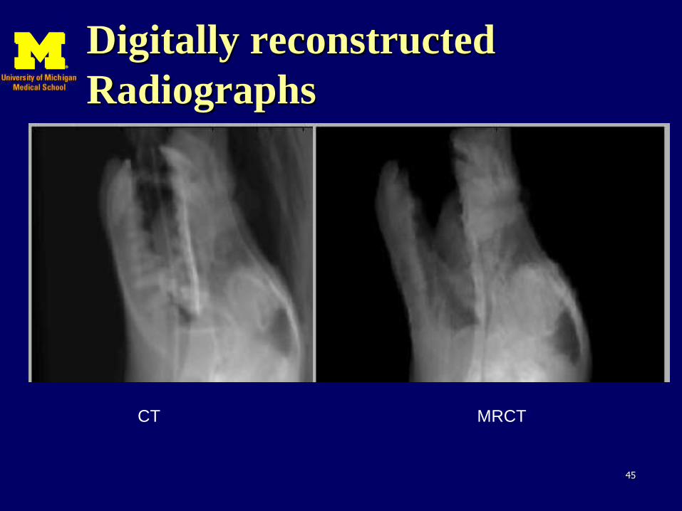
Digitally reconstructed

Radiographs

45

CT MRCT

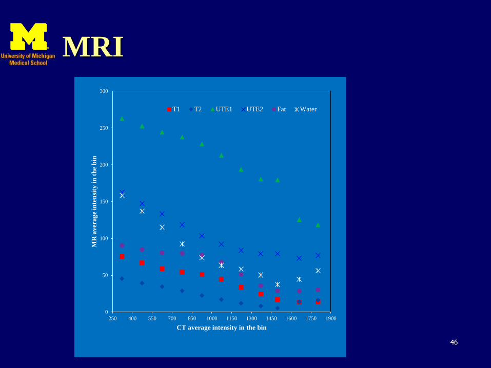
MRI

46

0

50

100

150

200

250

300

250 400 550 700 850 1000 1150 1300 1450 1600 1750 1900

MR

av

era

ge

inte

nsi

ty i

n t

he

bin

CT average intensity in the bin

T1 T2 UTE1 UTE2 Fat Water

47

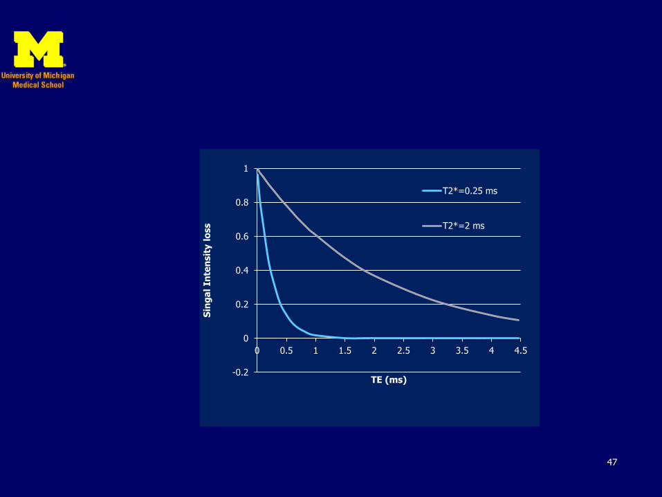
-0.2

0

0.2

0.4

0.6

0.8

1

0 0.5 1 1.5 2 2.5 3 3.5 4 4.5

Sin

ga

l In

ten

sit

y l

oss

TE (ms)

T2*=0.25 ms

T2*=2 ms

48

First volunteer MRCT

(UTE, no CT)

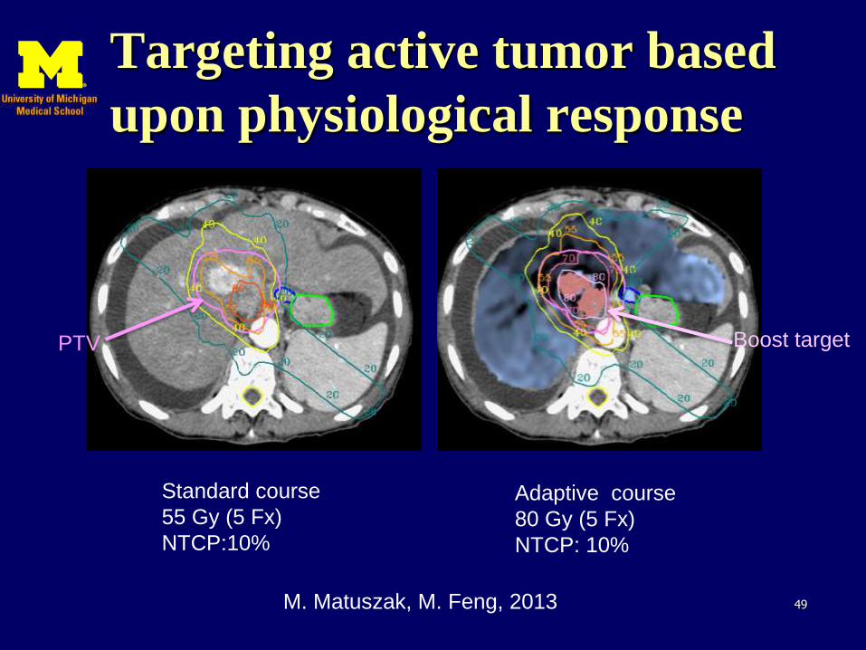
Targeting active tumor based

upon physiological response

49

Standard course

55 Gy (5 Fx)

NTCP:10%

Adaptive course

80 Gy (5 Fx)

NTCP: 10%

M. Matuszak, M. Feng, 2013

PTV Boost target

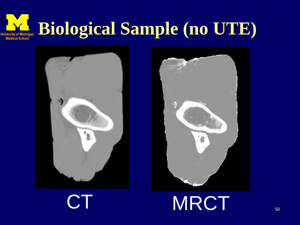
Biological Sample (no UTE)

50 CT MRCT