Chemical and Biological Engineering

MPC Introduction

B. Wayne Bequette

• Overview• Basic Concept of MPC• History

• Optimization Formulation• Models• Analytical Solution to Unconstrained Problem

• Summary• Limitations & a Look Ahead

B. Wayne Bequette

Motivation: Complex Processes

LC

PC

PC PC PC

LC LC

LC

cooling water

Toluene

Hydrogen

purge Hydrogen, Methane

fuel gas

steam

steamsteam

Diphenyl

Benzene product

CH4

Recycle Toluene

CC

TC

TCReactor

Rec

ycle

Col

umn

Ben

zene

Col

umn

Stab

ilize

r

Flas

h

Recycle Compressor

cooling water

CW

CW

quenchTC

LC LC

LCTC

open

FC

FC

FC

FC

TC

CC

TC

B. Wayne Bequette

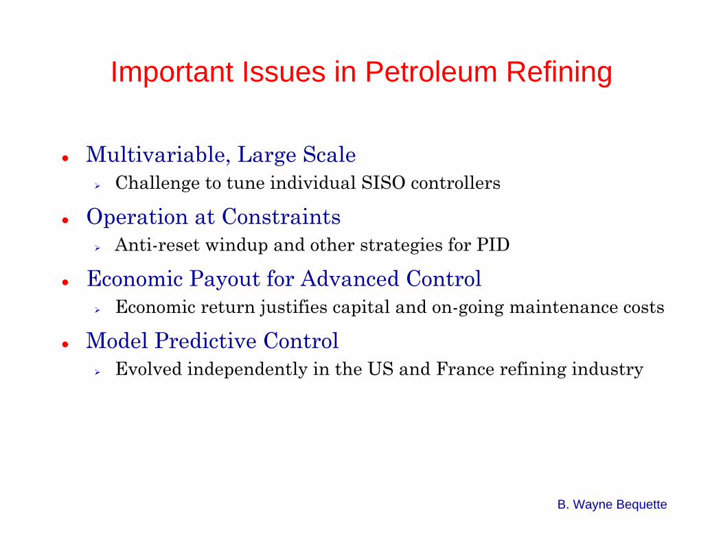
Important Issues in Petroleum Refining

Multivariable, Large ScaleChallenge to tune individual SISO controllers

Operation at ConstraintsAnti-reset windup and other strategies for PID

Economic Payout for Advanced ControlEconomic return justifies capital and on-going maintenance costs

Model Predictive ControlEvolved independently in the US and France refining industry

B. Wayne Bequette

How is MPC used?Unit 1 - PID Structure

Global Steady-StateOptimization(every day)

Local Steady-StateOptimization(every hour)

DynamicConstraintControl(every minute)

SupervisoryDynamicControl(every minute)

Basic DynamicControl(every second)

Plant-Wide Optimization

Unit 1 Local Optimization Unit 2 Local Optimization

High/Low Select Logic

PID Lead/Lag PID

SUM SUM

ModelPredictiveControl(MPC)

Unit 1 Distributed ControlSystem (PID)

Unit 2 Distributed ControlSystem (PID)

FCPC

TCLC

FCPC

TCLC

Unit 2 - MPC Structure

From Tom Badgwell, 2003 Spring AIChE Meeting, New Orleans

B. Wayne Bequette

Model Predictive Control (MPC)

t kcurrent step

setpoint

yactual outputs (past)

PPrediction Horizon

past control moves

u

max

min

MControl Horizon

past future

model prediction

t k+1current step

setpoint

yactual outputs (past)

PPrediction Horizon

past control moves

u

max

min

MControl Horizon

model prediction from k

new model prediction

Find current and future manipulated inputs that best meet a desired future output trajectory. Implement first “control move”.

Type of model for predictions?Information needed at step k for predictions?Objective function and optimization technique?Correction for model error?

Chapter 16

B. Wayne Bequette

Model Predictive Control (MPC)

t kcurrent step

setpoint

yactual outputs (past)

PPrediction Horizon

past control moves

u

max

min

MControl Horizon

past future

model prediction

t k+1current step

setpoint

yactual outputs (past)

PPrediction Horizon

past control moves

u

max

min

MControl Horizon

model prediction from k

new model prediction

At next sample time:

Correct for model mismatch,then perform new optimization.

This is a major issue –“disturbances” vs. model uncertainty

Find current and future manipulated inputs that best meet a desired future output trajectory. Implement first “control move”.

B. Wayne Bequette

MPC HistoryIntuitive

Basically arose in two different “camps”

Dynamic Matrix Control (DMC)1960’s and 1970’s – Shell Oil - US

Related to techniques developed in France (IDCOM)Large-scale MIMOFormulation for constraints important

Generalized Predictive Control (GPC)Evolved from adaptive controlFocus on SISO, awkward for MIMO

Charlie Cutler

(1976)

B. Wayne Bequette

Objective Functions

( ) ∑∑−

=+

=++ Δ+−=

1

0

2

1

2ˆM

iik

P

iikik uwyrJ

Quadratic Objective Function, Prediction Horizon (P) = 3, Control Horizon (M) = 2

With linear models, results in analytical solution (w/o constraints)

General Representation of a Quadratic Objective Function

( ) ( ) ( )2

12

233

222

211 ˆˆˆ

+

++++++

Δ+Δ+

−+−+−=

kk

kkkkkk

uwuw

yryryrJ

Weight 2 control moves

3 steps into future

B. Wayne Bequette

Alternative Objective Functions

( ) ∑∑−

=+

=++ +−=

1

0

2

1

2ˆM

iik

P

iikik uwyrJ

∑∑−

=+

=++ Δ+−=

1

01

ˆM

iik

P

iikik uwyrJ

Penalize u rather than Δu

Sum of absolute values (results in LP)

Will usually result in “offset”

Existing LP methods are efficient, but solutions hop from one constraint to another

B. Wayne Bequette

Models

State SpaceARX (auto-regressive, exogenous input)Step ResponseImpulse (Pulse) Response

Nonlinear, Fundamental (First-Principles)ANN (Artificial Neural Networks)Hammerstein (static NL with linear dynamics)VolterraMultiple Model

B. Wayne Bequette

Discrete Linear Models used in MPC

∞−∞+−−+−−

∞

=−

+++++=

=∑kNNkNNkNk

iikik

uhuhuhuh

uhy

LL 1111

1

kk

kkk

Cxyuxx

=Γ+Φ=+1 State Space

Input-Output(ARX)mkmkkk

nknkkk

ububububyayayay

−−−

−−−

+++++−−−−=

L

L

22110

2211

Step Response

usually b0 = 0

Some texts/papers have different sign conventions

Impulse Response

∞−∞+−−+−−

∞

=−

Δ++Δ+Δ++Δ=

Δ=∑kNNkNNkNk

iikik

usususus

usy

LL 1111

1

B. Wayne Bequette

-2 0 2 4 6 8

0

0.5

1

1.5

2

temp, deg C

discrete-time step

-2 0 2 4 6 8

0

0.2

0.4

0.6

0.8

1

discrete-time step

psig

s 1

ss

s

s

2

4 53

Etc.

S = s1 s2 s3 s4 s5 L sN[ ]T

Example Step Response Model

Used inDMC

B. Wayne Bequette

-2 0 2 4 6 8 10

0

0.2

0.4

0.6

0.8

1

discrete-time step

psig

-2 0 2 4 6 8 10-0.2

0

0.2

0.4

0.6

0.8

1

discrete-time step

temp, deg Ch

hh

1 2

3

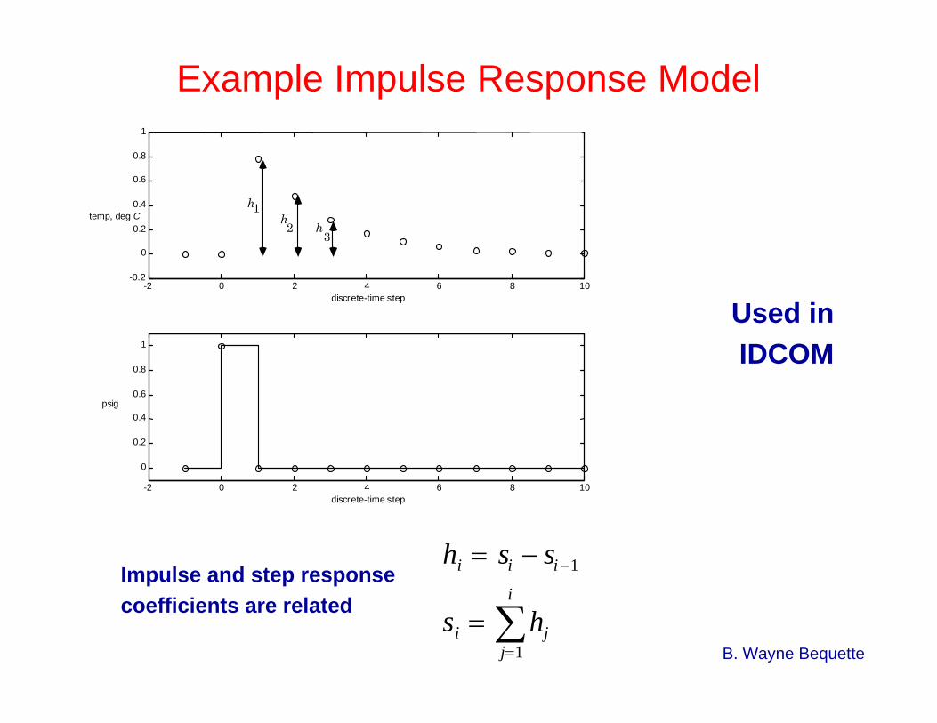
hi = si − si−1

si = hjj=1

i

∑

Example Impulse Response Model

Impulse and step responsecoefficients are related

Used inIDCOM

B. Wayne Bequette

Step & Impulse Models from State Space Models

ΓΦ= −1ii CH

∑∑==

− =ΓΦ=k

ii

k

i

ik HCS

11

1

kk

kkk

Cxyuxx

=Γ+Φ=+1

B. Wayne Bequette

MPC based on State Space Models

kk

kkk

xCyuxx

1

=Γ+Φ=+

with known current state, easy to propagate estimates

kkkk

kkk

uCxCCxyuxx

Γ+Φ==Γ+Φ=

++

+

11

1

and, using control changes

kkkk

kkk

uCuCxCyuuu

ΓΔ+Γ+Φ=Δ+=

−+

−

11

1

B. Wayne Bequette

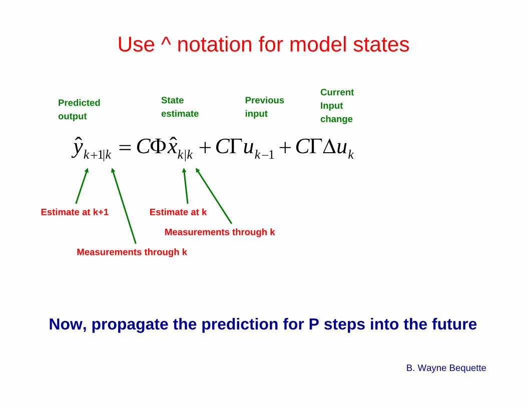
Use ^ notation for model states

kkkkkk uCuCxCy ΓΔ+Γ+Φ= −+ 1||1 ˆˆ

Measurements through k

Estimate at k+1 Estimate at k

Measurements through k

Predicted output

Stateestimate

Previousinput

CurrentInputchange

Now, propagate the prediction for P steps into the future

B. Wayne Bequette

Output Predictions

44444444 344444444 21

M

L

MM

L

44444 344444 21

MMM

response "forced"

1

1

1

1

1

1

1

made) are moves control more no (if response" unforced"or "free"

1

1

1

|

2

|

|2

|1

0000

ˆ

ˆ

ˆˆ

⎥⎥⎥⎥

⎦

⎤

⎢⎢⎢⎢

⎣

⎡

Δ

ΔΔ

⎥⎥⎥⎥⎥⎥

⎦

⎤

⎢⎢⎢⎢⎢⎢

⎣

⎡

ΓΦΓΦ

ΓΓ+ΦΓΓ

⎥⎥⎥⎥⎥

⎦

⎤

⎢⎢⎢⎢⎢

⎣

⎡

ΓΦ

Γ+ΦΓΓ

+

⎥⎥⎥⎥

⎦

⎤

⎢⎢⎢⎢

⎣

⎡

Φ

ΦΦ

=

⎥⎥⎥⎥⎥

⎦

⎤

⎢⎢⎢⎢⎢

⎣

⎡

−+

+

−

=

−

=

−

−

=

−

+

+

+

∑∑

∑

Mk

k

k

P

i

iP

i

i

kP

i

i

kk

PkPk

kk

kk

u

uu

CC

CCCC

u

C

CCC

x

C

CC

y

yy

fSfuΔ

fY

B. Wayne Bequette

Output Predictions

444444 3444444 21

M

L

MM

L

444 3444 21

MMM

response "forced"

1

1

11

12

1

made) are moves control more no (if response" unforced"or "free"

12

1

|

2

|

|2

|1

0000

ˆ

ˆ

ˆˆ

⎥⎥⎥⎥

⎦

⎤

⎢⎢⎢⎢

⎣

⎡

Δ

ΔΔ

⎥⎥⎥⎥

⎦

⎤

⎢⎢⎢⎢

⎣

⎡

⎥⎥⎥⎥

⎦

⎤

⎢⎢⎢⎢

⎣

⎡

+

⎥⎥⎥⎥

⎦

⎤

⎢⎢⎢⎢

⎣

⎡

Φ

ΦΦ

=

⎥⎥⎥⎥⎥

⎦

⎤

⎢⎢⎢⎢⎢

⎣

⎡

−+

+

+−−

−

+

+

+

Mk

k

k

MPPP

k

P

kk

PkPk

kk

kk

u

uu

SSS

SSS

u

S

SS

x

C

CC

y

yy

fSfuΔ

fY

Step response coefficients

B. Wayne Bequette

Optimization Problem

( ) ( ) Tik

M

i

uTik

P

ikikkik

yTkikkiku

uWuyrWyrJf

+

−

=+

=++++Δ

ΔΔ+−−= ∑∑1

01|||| ˆˆmin

⎥⎥⎥

⎦

⎤

⎢⎢⎢

⎣

⎡

=y

y

Y

W

WW

000000

O

⎥⎥⎥

⎦

⎤

⎢⎢⎢

⎣

⎡

=u

u

U

W

WW

000000

O

EWE YT ˆˆf

UTf uWu ΔΔ

Where

ff uSfrYrE Δ−−=−= ˆˆ

E

ff uSEE Δ−=ˆ

and

so

“unforced” (freeresponse) error

future setpoints

B. Wayne Bequette

Optimization Problem

( ) ( )ff

YTf

Tf

YTf

Tf

YT

ffYT

ffYT

uSWSuEWSuEWE

uSEWuSEEWE

ΔΔ+Δ−=

Δ−Δ−=

2

ˆˆ

fUT

f uWu ΔΔ+=Δ

Jfu

min EWE YT ˆˆ

( ) EWSuuWSWSu YTf

Tff

Uf

YTf

Tf Δ−Δ+Δ 2=

ΔJ

fumin

so

can be written

0=Δ∂∂ fuJ

and the unconstrained solution is found from

B. Wayne Bequette

Unconstrained Solution

In practice, do not actually invert a matrix. Solve asset of simultaneous equations (or use \ in MATLAB)

( ) EWSWSWSu YTf

Uf

YTff \+=Δ

Analytical Solution for Unconstrained System

( ) EWSWSWSu YTf

Uf

YTff

1−+=Δ

“unforced” error

B. Wayne Bequette

Vector of Control Moves

43421

M

moves future andcurrent

1

1

⎥⎥⎥⎥

⎦

⎤

⎢⎢⎢⎢

⎣

⎡

Δ

ΔΔ

=Δ

−+

+

Mk

k

k

f

u

uu

u

Although a set of control moves is computed, only thefirst move is implemented

The next output at k+1 isobtained, then a new optimization problem is solved

kuΔ

B. Wayne Bequette

MPC Tuning Parameters

Prediction Horizon, P

Control Horizon, M

Manipulated Input Weighting, Wu

Usually, P >> M for robustness (less aggressive action). Sometimes M = 1, with P varied for desired performance.

Sometimes larger input weights for robustness

B. Wayne Bequette

CainF

CbF

Example Inverse Response Process: Van de Vusse

Constant V,T, ρ

A B Ck1 k2

A+A Dk3

dCadt = -k1Ca - k3Ca2 + (Cain - Ca)u

dCbdt = k1Ca - k2Cb - Cbu where u = F/V

B. Wayne Bequette

Example: Inverse Response Process

0 10 20 30 40 50-0.1

0

0.1

0.2

0.3

0.4

0.5

0.6

discrete time index, i

s(i)

step response coefficients

First four coefficients are negative

Sum of first eight coefficients is positive

B. Wayne Bequette

Closed-Loop: Compare P=10, M=1 with P=25, M=1

0 1 2 3 4 5 6-0.5

0

0.5

1

1.5

y, m

ol/l

time, min

0 1 2 3 4 5 6

0

1

2

3

u, m

in- 1

time, min

P = 10, M = 3P = 25, M = 1

P = 10, M = 3P = 25, M = 1

Short prediction horizons &long control horizons leadto more aggressive action

B. Wayne Bequette

Results

0 1 2 3 4 5 6-1.5

-1

-0.5

0

0.5

1

1.5

y, m

ol/l

time, min

P = 8P = 7

0 1 2 3 4 5 6-6

-4

-2

0

2

u, m

in- 1

time, min

P = 8P = 7

Control Horizon: M = 1, Weighting: W = 0

P=7:Unstable

B. Wayne Bequette

Stability of Inverse Response Systems with DMC

For a control horizon, M = 1, closed-loop MPC will be stable for a prediction horizon where the sum of the impulse response coefficients has the same sign as the process gain

0min

1>∑

=

P

iis

For the example, Pmin = 8, so P = 7 = unstable

B. Wayne Bequette

Summary

Concise overview of MPC

State space model, unconstrained solution

Have not discussedState estimation and “corrected outputs”DisturbancesConstraintsOther model forms