Moving Mesh Methods for Singular Problems on a

Sphere Using Perturbed Harmonic Mappings

Yana Di ∗, Ruo Li †, Tao Tang ‡and Pingwen Zhang §

March 14, 2006

Abstract

This work is concerned with developing moving mesh strategies for solving prob-

lems defined on a sphere. To construct mappings between the physical domain and

the logical domain, it has been demonstrated that harmonic mapping approaches are

useful for a general class of solution domains. However, it is known that the curvature

of the sphere is positive, which makes the harmonic mapping on a sphere not unique.

To fix the uniqueness issue, we follow Sacks and Uhlenbeck [Ann. Math., 113, 1-24

(1981)] to use a perturbed harmonic mapping in mesh generation. A detailed moving

mesh strategy including mesh redistribution and solution updating on a sphere will

be presented. The moving mesh scheme based on the perturbed harmonic mapping

is then applied to the moving steep front problem and the Fokker-Plank equations

with high potential intensities on a sphere. The numerical experiments show that

with a moderate number of grid points our proposed moving mesh algorithm can

accurately resolve detailed features of singular problems on a sphere.

1 Introduction

In this work, we will consider efficient moving mesh methods for solving singular problems

on a sphere. Partial differential equations (PDEs) defined on a sphere are seen in many

∗LMAM & School of Mathematical Sciences, Peking University, Beijing 100871, P. R. China, email:

dyn@math.pku.edu.cn.†LMAM & School of Mathematical Sciences, Peking University, Beijing 100871, P. R. China, email:

rli@math.pku.edu.cn.‡Mathematics Department, Hong Kong Baptist University, Kowloon Tong, Hong Kong, email:

ttang@math.hkbu.edu.hk. The research of this author was supported in part by Hong Kong Research

Grants Council and the International Research Team on Complex System of Chinese Academy of Sciences.§LMAM & School of Mathematical Sciences, Peking University, Beijing 100871, P. R. China, email:

pzhang@math.pku.edu.cn. The research of this author was supported in part by the special funds for

Major State Research Projects and National Science Foundation of China for Distinguished Young Scholars.

1

practical cases such as polymer rheological analysis, ocean modeling, and global climate

simulation. The moving mesh technique is one of the natural choices for solving problems

with localized moving singularities. Examples include moving internal boundaries or in-

terfaces separating different regions which are present in many problems in nature, such as

interfaces separating two different fluids in a multiphase flow, and between solid and liquid

regions in a solidification process. Such interfaces are in general dynamic, i.e. they evolve in

time. Moving mesh methods have been proved powerful for solving time-dependent partial

differential equations in two-dimensional domains and simple three-dimensional domains

([2, 3, 4, 5, 24, 30, 31, 34]).

In general, a moving mesh method always involves a logical domain and a physical

domain, together with a transformation between them. In [12], Dvinsky suggests that

harmonic function theory may provide a general framework for developing useful mesh

generators. His method can be viewed as a generalization and extension of Winslow’s

method [33]. However, unlike most other generalizations which add terms or functionals

to the basic Winslow grid generator, his approach uses a single functional to accomplish

the adaptive mapping. The critical points of this functional are harmonic maps. Meshes

obtained by Dvinsky’s method enjoy desirable properties of harmonic maps, particularly

regularity, or smoothness [15, 27]. Motivated by the work of Dvinsky, a moving mesh finite

element strategy based on harmonic mapping was proposed and studied by the authors in

[21]. The key idea of this strategy is to construct the harmonic map between the physical

space and a parameter space by an iteration procedure.

For two-dimensional domains or three-dimensional cubic domains as considered in [21,

22], the metric on the logical domain is Euclidean. Consequently, the construction of the

harmonic mapping only solves some linear equations. However, this is not the case for

spherical problems. In fact, if the physical domain is a sphere then it is natural to set

the logical domain as a sphere rather than a convex polygon as used in [21]. In this case,

the fact that the curvature of a sphere is positive makes the harmonic mapping on sphere

not unique. Another difficulty is that the metric on the unit sphere is not an identity

anymore, which is different from the cases considered before, see, e.g. [21]. Our goal is to

construct a transformation which preserves the good properties of the harmonic mappings

such as smoothness and uniqueness. Moreover, a scheme for solving the nonlinear equation

induced by the metric on a sphere will be designed,

Motivated by the work of Sacks and Uhlenbeck [26], we will use the so-called per-

turbed harmonic mapping to construct a unique mapping between the physical and logical

space. It will be seen that the perturbed harmonic mappings are useful for handling spher-

ical domains. The nonlinear Euler-Lagrange equations from minimizing the mesh energy

functional will be solved by a local Gauss-Seidel-like iterative method. The numerical ex-

periments indicate that a satisfactory approximation to the perturbed harmonic mapping

can be obtained using only a few iteration steps. Furthermore, a key step for the moving

mesh method is to obtain an improved new mesh based on the underlying numerical solu-

2

tions and the old meshes. With the spherical geometry, the mesh redistribution has to be

designed carefully: efforts have to be made to ensure that the mesh movement occurs only

on the sphere, and that all the grid points stay on the sphere during the whole process of

mesh redistribution. In this work, appropriate mesh redistribution and solution updating

strategies will be investigated.

The rest of the paper is arranged as follows. In Section 2, the theory of the perturbed

harmonic mapping on a sphere will be briefly reviewed. Section 3 describes the general

framework of the moving mesh method on a sphere, including some details of the mesh-

redistribution and solution-updating strategies. In Section 4, the proposed moving mesh

scheme will be applied to solve moving shocks on a sphere and the Fokker-Planck equations

derived from liquid crystal simulations. For the latter problem, the solutions of the problem

tend to a delta function when the strength of the excluded volume potential is large (see

[20]). With a uniform mesh, an extremely fine mesh is required in order to obtain reasonable

resolution, but the efficiency can be enhanced significantly by using moving mesh methods.

Some concluding remarks will be given in the final section.

2 Perturbed Harmonic Mapping

Let Ω and Ωc be compact Riemannian manifolds of dimension n with metric tensors dij

and rαβ in some local coordinates ~x and ~ξ, respectively. The energy density of a mapping~ξ : ~x 7→ ~ξ, is defined by

e(~ξ) = Gijgαβ

∂ξα

∂xi

∂ξβ

∂xj, (2.1)

where the standard summation convention is assumed. The corresponding energy func-

tional is then defined by

E(~ξ) =

∫

Ω

e(~ξ)dx. (2.2)

The harmonic mapping is the mapping which minimizes the above energy functional.

Existence and uniqueness of the harmonic map are guaranteed provided that the Rie-

mannian curvature of Ωc is non-positive and its boundary is convex (see Hamilton-Schoen-

Yau [15, 27]). However, this result does not apply to the case when the physical and

logical domains are a sphere, i.e., Ω = Ωc = S2; in this case, the Riemannian curvature of

Ωc is positive. In fact, the energy functional (2.2) has the conformal invariance [26], which

leads to non-uniqueness of the harmonic mappings. To recover the uniqueness, we follow

the work of Sacks and Uhlenbeck [26] to employ a so-called perturbed harmonic mapping

approach. More precisely, let

Eα(~ξ) =

∫

Ω

(1 + e(~ξ))αdx, (2.3)

with α > 1. It is noted that when α = 1 the functionals (2.3) and (2.2) are equivalent. It

3

is known that the Sobolev space of mappings:

L2α1 (M, N) = ξ ∈ L2α

1 (M, Rk) : ξ(x) ∈ N ⊂ C0(M, N), (2.4)

is an C2 separable Banach manifold for α > 1 [25]. In particular, it is shown in [26] that

if α > 1, then the critical mappings of Eα in L2α1 (M, N) are C∞ and are unique in the

sense of isometric transformation. Such regularity and uniqueness results provide a sound

theoretical background for the moving mesh method based on the perturbed harmonic

mappings.

The Euler-Lagrange equation of the energy functional (2.3) is given by

−∆L−Bξl − (α− 1)∇|∇ξ|2 · ∇ξl

|∇ξ|2 + [A(ξ)(dξ, dξ)]l = 0, (2.5)

where ∆L−B stands for the Laplace-Beltrami operator:

∆L−Bf =1√G

∑

i,j

∂

∂xi

(√GGij ∂f

∂xj

)

,

and A(ξ) is the second fundamental form of Ωc. For a sphere, it is known that

A(ξ)(dξ, dξ) = −|∇ξ|2ξ. (2.6)

Moreover, the derivatives in curvilinear coordinates are given by

(∇ξm)j = Gij ∂ξm

∂xi,

(

∇|∇ξ|2)j

= Gij ∂

∂xi

(

∑

t

Gkl ∂ξt

∂xk

∂ξt

∂xl

)

.

Consequently, the Euler-Lagrange equation (2.5) can be written in the following divergence

form:

−∇ ·(

α|∇ξ|2(α−1)∇ξl)

+ α|∇ξ|2(α−1)[A(ξ)(dξ, dξ)]l = 0. (2.7)

Using the Stokes law, we can get the weak form of the above equation:∫

S2

∑

l

|∇ξ|2(α−1)∇ξl · ∇λl −∑

l

|∇ξ|2αξlλl

dV = 0, ∀λ ∈ L2α1 (M, N). (2.8)

The way of obtaining the mapping for the perturbed equation (2.7) is similar to that used

for obtaining the conventional harmonic mappings described in [21, 22]. It is shown that

with the harmonic mappings the metric distortion can be minimized [13, 26]. Moreover, it

is expected that the mesh associated with the mapping (2.7) has certain smoothness and

uniqueness.

In this work, the perturbed harmonic mapping will be used to generate adaptive meshes

for unstructured triangles in spherical domains. We point out that there are several other

successful ways for adaptive re-meshing also by minimizing mesh energy function that

depends on the local physical scales, see, e.g., Anderson et al. [1], Liao et al [23], Sun &

Huang [17], and Wang & Wang [32].

4

3 Moving Mesh Methods for Spherical Domain

Consider the time-dependent PDEs on a sphere Ω = S2,

Ψt = L(Ψ) in Ω× (0, T ], (3.1)

where L is some spatial partial differential operator, with initial value

Ψ|t=0 = Ψ0, in Ω. (3.2)

Let us consider a moving mesh method based on the perturbed harmonic mappings to solve

this time-dependent problem. We triangulate the domain Ω into a mesh Th with spherical

triangular elements. The equation (3.1) is discretized with finite element approximation

on the mesh Th. Assume a PDE solver is given so that the numerical solution at time level

tn+1 can be obtained by using the numerical approximation at t = tn. Since our mesh

varies with respect to time, we denote the mesh at time step tn as T (n)h . The procedure to

combine the mesh motion and the PDE solutions is illustrated below:

• Step 0: Initialization. Set n = 0 and t0 = 0. Project the initial function on the initial

mesh T (0)h , which gives Ψ

(0)h ;

• Step 1: Solution evolution. Obtain the numerical solutions at t = tn+1 on the mesh

T (n)h by an appropriate PDE solver, to obtain Ψ

(n+1)h ;

• Step 2: Mesh quality evaluation. Check the mesh quality by certain criteria; if satis-

factory, set T (n+1)h = T (n)

h , n = n + 1, and go to Step 1;

• Step 3: Mesh quality enhancement. Obtain a more appropriate mesh by some mesh

moving techniques, as described later in this section;

• Step 4: Solution updating. Update the numerical solution Ψ(n+1)h on the new mesh

obtained in Step 3 and go to Step 2.

We point out that the mesh quality (mentioned in Step 2 above) takes into account

the shape, alignment and adaptation features of the elements. For example, the minimum

angle, the maximum angle, and the aspect ratio have been used widely to characterize the

mesh quality. More details can be found in Huang [18].

3.1 Finite element space on sphere

The sphere is triangulated into a mesh with spherical triangular elements. The Voronoi

spherical geodesic grid (see, e.g. [11]) is used in our work. Here we give a finite element

space for the discretization of the problem (3.1)-(3.2). We will project the linear basis

functions of the triangles on polyhedron onto the spherical geodesic triangles. The vertices

5

O

A

C

B

P

W

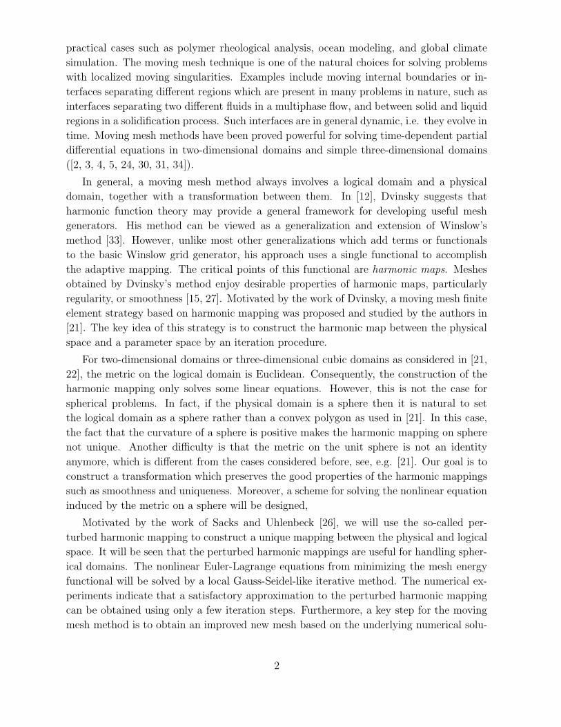
Figure 1: The shape function defined on a spherical triangle.

(anti-clockwise) of a spherical geodesic triangle K are denoted by A, B and C. The plane

triangle Kp has the same vertices. For a point P ∈ K, the intersection point of line−→OP

and Kp is denoted by W (see Figure (3.1) ). The three basis functions on spherical geodesic

triangle K are defined by

λ1(~x) =1

D(~w · ~a2 × ~a3),

λ2(~x) =1

D(~w · ~a3 × ~a1),

λ3(~x) =1

D(~w · ~a1 × ~a2),

(3.3)

where

−→OA = ~a1,

−−→OB = ~a2,

−→OC = ~a3,

−→OP = ~x,

−−→OW = ~w, D = (~a1 · ~a2 × ~a3), ~w(~x) = D

~x

~x · ~d,

~d = ~a1 × ~a2 + ~a2 × ~a3 + ~a3 × ~a1.

With these notations, a finite element space on sphere is presented:

Hh ,

Ψh ∈ C0 (Ω) : Ψh|K ∈ span λ1, λ2, λ3 , ∀K

. (3.4)

6

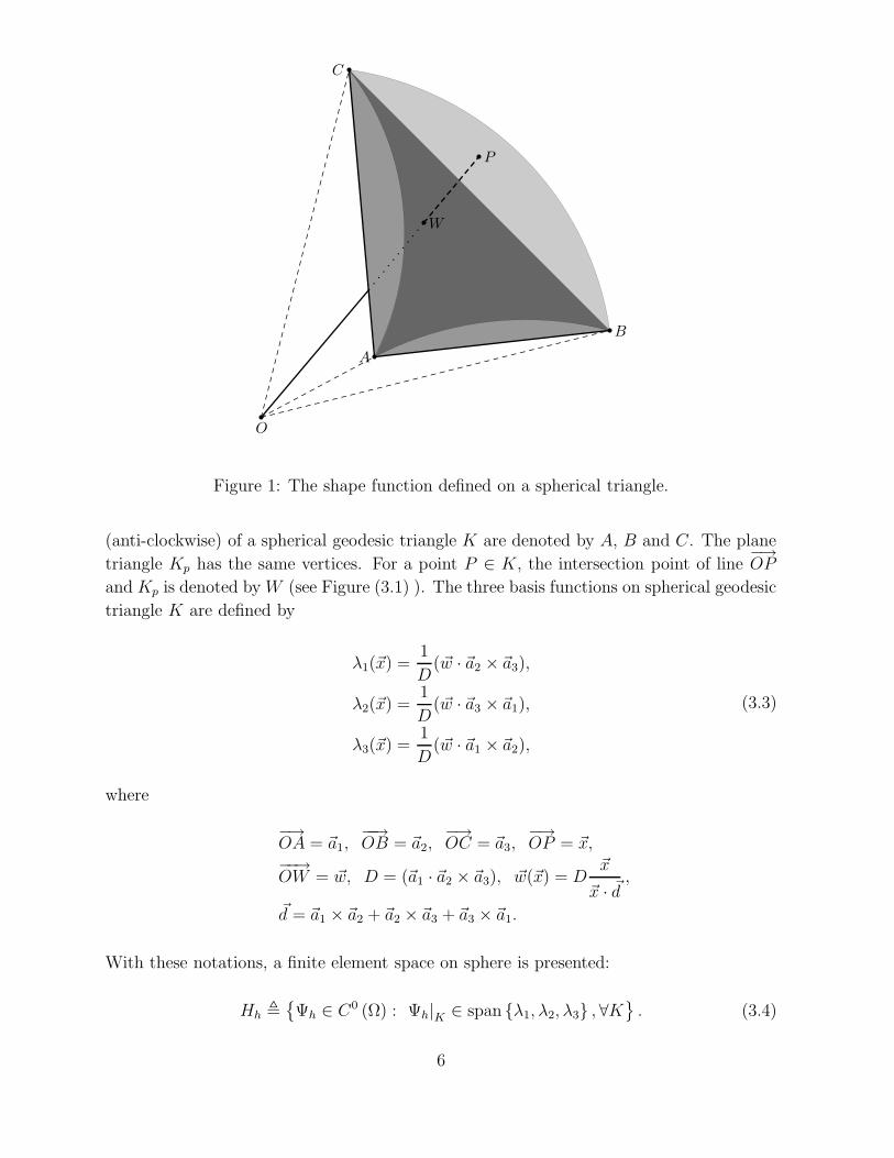
3.2 Mesh redistribution on sphere

A key step for the moving mesh method is to obtain an improved new mesh based on the

underlying numerical approximations. In our computations, we simply choose the given

physical domain, i.e., the sphere, as the logical domain, and we use the Voronoi spherical

geodesic grid (see, e.g., [11]) to generate a quasi-uniform mesh with triangular elements on

the logical domain. Obviously, this also gives the initial partition for the physical domain.

The nodes in the physical mesh are denoted by Xi, 1 ≤ i ≤ N , and the nodes in the

logical mesh by Ξi, 1 ≤ i ≤ N . Initially, since we choose the logical mesh the same as the

physical mesh, we have Ξi = Xi. The physical mesh will be redistributed at each time step,

while the logical mesh will be kept unchanged during the entire process of the numerical

computations. For each time step, by numerically solving the Euler-Lagrange equation

(2.7), we can obtain a discrete transformation between the physical domain ~xh and the

logical domain ~ξh. The logical mesh is then given such that Ξi = ~ξh(Xi). The metric on

the physical domain is given according to the given PDEs and their numerical solution,

which is called monitor function.

On the sphere, there are no local coordinates to cover the whole domain S2. Therefore,

we have to choose suitable local coordinates. The metric for the logical domain is the natu-

ral metric of sphere as a sub-manifold embedded in R3. Since the Euler-Lagrange equation

(2.7) is nonlinear, it will be solved numerically by a point by point iterative approach. As-

sume that we are considering a node in the physical mesh, Xk, whose corresponding node

in the logical mesh is denoted by Ξk. Denote the set of triangles in the physical domain

with Xk as a vertex by Sk and the corresponding set in the physical domain by Sc,k. We

will set the local coordinate around Xk in the physical domain and the local coordinate

around Ξk in the logical domain. It is natural to eliminate one component whose absolute

value is the largest among the three components. This will give two-dimensional local

coordinates. For example, for Xk = (x1k, x

2k, x

3k) set, if |x1

k| ≥ |x2k| and |x1

k| ≥ |x3k| then

we will let (x1k, x

2k) ← (x2

k, x3k) to be the local coordinate around Xk. The same strategy

is employed to choose the local coordinate around Ξk. We then have the Euler-Lagrange

equation (2.7) around the node Ξk:

∇ ·(

|∇ξ|2(α−1)∇ξl)

+ |∇ξ|2αξl = 0 for l = 1, 2, 3,

ξ|∂Sk= ξb.

(3.5)

In the physical domain, around Xk the patch of surface on the unit sphere can be expressed

as(

x3)2

= 1−(

x1)2 −

(

x2)2

, (3.6)

and the metric of the physical domain is taken as a sub-manifold embedded in R3:

Giji,j=1,2 =

(

1− (x1)2

x1x2

x1x2 1− (x2)2

)

. (3.7)

7

The metric Gij on the physical domain around Xk is then set as

Gij = m(uh)Gij, (3.8)

where m(uh) is the monitor function given for the problem under consideration. The choice

of the monitor function m is very subtle, which is an indicator of the solution singularity

and is problem dependent. A general discussion of the monitor function can be found in

[6, 29].

Now on the patch of triangles Sk, we will solve a Dirichlet boundary-value problem

for (3.5), with linear boundary mapping segment-wise on ∂Sk determined by the vertex

mapping Ξn = ~ξ(Xn), ∀Xn ∈ Sk, n 6= k. The mapping in Sk is approximated by a piecewise

linear mapping on every triangle in Sk. Thus the mapping can be given only if ~ξ(Xk) is

given. Using the standard Galerkin approximation for (3.5) in Sk, we have only one test

function which is the pyramid-like basis function located at Xk. This gives

∫

Sk

|∇ξ|2(α−1)∇ξl · ∇λk − |∇ξ|2αξlλk

dV = 0 for l = 1, 2, 3, (3.9)

where λk is the test function for Xk, which is an algebraic system with order 2α + 1 for

three unknowns. We will solve (3.9) approximately. On Sk, we denote ~ξh by

~ξh =∑

n

Ξnλnh + Ξkλ

k , (3.10)

where the summation for n is taken over all vertices in Sk except Xk. By taking |∇ξ| in(3.9) explicitly, i.e., ξh in |∇ξ| takes the currently available Ξk as its value at Xk, we then

get an explicit approximation for (3.9):

Ξlk ≈

∫

Sk

∑

n

|∇ξ|2αΞlnλlλkdV −

∑

n

∫

Sk

|∇ξ|2(α−1)GijΞln

∂λn

∂xi

∂λk

∂xjdV

∫

Sk

(

−|∇ξ|2αλkλk + |∇ξ|2(α−1)Gij ∂λk

∂xi

∂λk

∂xj

)

dV

. (3.11)

Below we will describe the algorithm for mesh redistribution, which is similar to the one

proposed in [21]. In the first step, we iterate for k from 0 to N , using (3.11) to update all

logical nodes Ξk until convergence (i.e., the difference between the obtained Ξk and initial

(fixed) Ξ(0)k is smaller than a given tolerance). The tolerance for the convergence criteria is

of the order O(hl) where hl is the typical element size in the logical mesh. The converged

result is denoted by Ξ?k, and we then get the difference between Ξ?

k and the initial logical

mesh as

δΞk = Ξ(0)k − Ξ?

k. (3.12)

In the second step, we use the above difference to obtain the mesh redistribution informa-

tion in the physical mesh difference. Again we will choose the same local coordinate as

8

described above. For a node Xk in the physical mesh, we first compute the mesh motion

vector:

δX lk =

∑

K∈Sk

|E| ∂xl

∂~ξ

∣

∣

∣

∣

K

δΞk

∑

K∈Sk

|E|, for l = 1, 2, (3.13)

where the Jacobian matrix ∂~x/∂~ξ∣

∣

Kis computed by using the fact that the linear element

is used (see also [21]):

(

Ξ1E1− Ξ1

E0Ξ1

E2− Ξ1

E0

Ξ2E1− Ξ2

E0Ξ2

E2− Ξ2

E0

)

∂x1

∂ξ1

∂x1

∂ξ2

∂x2

∂ξ1

∂x2

∂ξ2

=

(

X1E1−X1

E0X1

E2−X1

E0

X2E1−X2

E0X2

E2−X2

E0

)

(3.14)

and E0, E1 and E2 are the subscripts of the three vertices of the element K in the physical

mesh. The coordinate in the third dimension is excluded, as explained earlier (i.e., with

the way of choosing the local coordinate). On the other hand, to ensure that the mesh

movement occurs only on the sphere, the third component can be recovered by using

δX3k → sgn(X3

k)

√

1− (X1k + δX2

k)2 − (X2

k + δX2k)

2 −X3k . (3.15)

In the third step, we will control the magnitude of each redistribution to avoid mesh

tangling. For the element K ∈ Th with vertices E0, E1 and E2, we solve the following cubic

equation (in terms of µ),

det(

XE0+ µ · δXE0

XE1+ µ · δXE1

XE2+ µ · δXE2

)

= 0, (3.16)

where δXEkis determined by (3.13). Denote the smallest positive root of (3.16) by µK.

The mesh motion parameter is then set as

µ? = minK∈Th

1; µK/2 . (3.17)

It is obvious that the mesh tangling can be avoided if we move the mesh using the formula

Xk ← Xk + µ?δXk.

In the last step, we update the mesh moving direction by

δXk ←Xk + µ?δXk

|Xk + µ?δXk|−Xk . (3.18)

This is to make sure that all the grid points are moving along the sphere. The new mesh

nodes are then given by Xk + δXk. It can be verified that the new nodes are all on the

sphere.

9

3.3 Solution interpolation on the new mesh

After redistributing the mesh in the physical domain Ω, we need to transfer the solution

information on the old mesh to the new mesh. Let δ~x :=∑N

i=1 δXiλi, where λi is the

basis function of Hh. Assume that a finite element solution Ψ(n)h =

∑N

i=1 Ψ(n)i λi is given

at t = tn. Let τ be a virtual time variable. We will regard the mesh motion from the old

mesh to the new mesh as a linear homotopy for τ goes from 0 to 1. Consequently, the

mesh flow with the virtual time τ is ~x(τ) , ~xold + τδ~x. For an arbitrary point ~x0 ∈ Th,

the basis function λi(~x) associated with ~x0 will be varying linearly with τ . Since λi(~x) is

defined on the physical mesh, it is denoted by λi(~x; τ). Direct calculation shows that

dλi(~x; τ)

dτ= δ~x · ∇~xλ

i(~x; τ). (3.19)

Assume that the numerical solution on mesh ~x(τ) is of the form

Ψh(~x; τ) =N∑

i=1

Ψi(τ)λi(~x; τ), (3.20)

which takes the starting value Ψh(·; 0) = Ψ(n)h . The main idea of the solution updating is

to let the variation of Ψh(·; τ) with respect to τ vanish in the test function space:

⟨

dΨh(·; τ)

dτ, Φh

⟩

= 0, ∀Φh ∈ Hh. (3.21)

Using (3.19) and (3.20) gives

N∑

i=1

∫

Ω

dΨi

dτλi(·; τ)λj(·; τ) + Ψiδ~x · ∇~xλ

i(·; τ)λj(·; τ)

dx = 0, 1 ≤ j ≤ N. (3.22)

The above ODE system can be solved by some appropriate ODE solver, e.g., a three-step

Runge-Kutta method ([21, 22]).

4 Numerical experiments

We first discuss the perturbation parameter α in (3.5): in the numerical computations

reported in this section it is chosen as 1.5. It is known [25] that α must be larger than 1 in

order to ensure the uniqueness of the mapping. If α is close to 1, the critical mapping of

Eα is close to a harmonic mapping. This implies that α should be chosen approximately

1. On the other hand, it is found that larger values of α increase the solution efficiency

for (2.8). In fact, larger values of α can speed up the convergence of the mesh movement:

note that the nonlinear Euler-Lagrange equations are solved by a local Gauss-Seidel-like

iterative method. With a few numerical tests, it is found that one of the good choices for

the parameter α should be approximately 1.5.

10

Example 4.1 (Moving steep front on a sphere) Our first example is to compute a

moving steep front along the direction ~b := (1, 1, 1)T governed by the following equation:

∂Ψt + Ψ~b · ∇∗Ψ = ε∆L−BΨ, (4.1)

which is defined on the unit sphere, where ∇∗ is the surface gradient. The initial condition

is given by

Ψ(x, y, z; 0) =

(

1 + exp(x + y + z + 1

2ε)

)−1

. (4.2)

We first briefly discuss the PDE algorithm to be used. For this example, a simple finite

element discretization as described in Section 3.1 is employed. The weak formulation of

the equation (4.1) reads: Find Ψ ∈ H1(Ω) such that

∫

Ω

∂Ψ

∂tvdx +

∫

Ω

Ψ~b · ∇∗Ψvdx = −ε

∫

Ω

∇∗Ψ · ∇∗vdx, ∀v ∈ H1(Ω). (4.3)

In the finite element space Hh, the above weak form can be approximated as: Find Ψh ∈ Hh,

such that∫

Ω

∂Ψh

∂tvhdx +

∫

Ω

Ψh~b · ∇∗Ψhvhdx = −ε

∫

Ω

∇∗Ψh · ∇∗vhdx, ∀vh ∈ Hh(Ω). (4.4)

For the temporal approximation, an explicit three-step Runge-Kutta scheme is applied,

see, e.g., [7].

In our computations, the viscosity coefficient ε is chosen as 0.01. For the convection

dominant problem, more mesh points are required around the wave front, which makes the

use of the moving mesh methods meaningful. The monitor function m defined in (3.8) is

taken as the standard gradient-based one, i.e.,

m(Ψ) =√

1 + β|∇Ψ|2. (4.5)

For problems with moving steep front, the parameter β has to be set as a large number,

say between 102 to 103; see, e.g., [6]. A large value of β can usually cluster more grid points

around the steep front. On the other hand, if |∇Ψ| in (4.5) is replaced by |∇Ψ|/ maxΩ |∇Ψ|then the parameter β can be chosen as an O(1) number, see, e.g., [7]. In our computations,

the parameter β in (4.5) is chosen as 103.

In Fig. 2, the moving meshes obtained by using our moving mesh scheme with 800 nodes

(about 1600 triangular elements) are plotted. Together in this figure are the numerical

solutions for Ψ at various time levels. Fig. 2(a) shows the initial state: the initial front

is at x + y + z + 1 = 0, where a stage can be seen. The solution is 0 on the left-top side

of the front and 1 on the right-bottom side. It can be seen that the front moves along

the direction (1, 1, 1)T on the sphere. In Figs. 2(b)-(f), the area with solution value 1

becomes bigger, and the area of value 0 becomes smaller as time increases. At t = 1.5, the

solution is mostly 1 on the sphere and is 0 only on a small concave area. In order to display

11

the numerical solution more clearly, the figures are plotted from various visual angles at

different time levels. Moreover, in order to have a better idea of the mesh distribution the

meshes are projected to a planisphere and are plotted in Fig. 3. It is seen that our moving

mesh scheme adapts the mesh extremely well in the regions with large solution gradients.

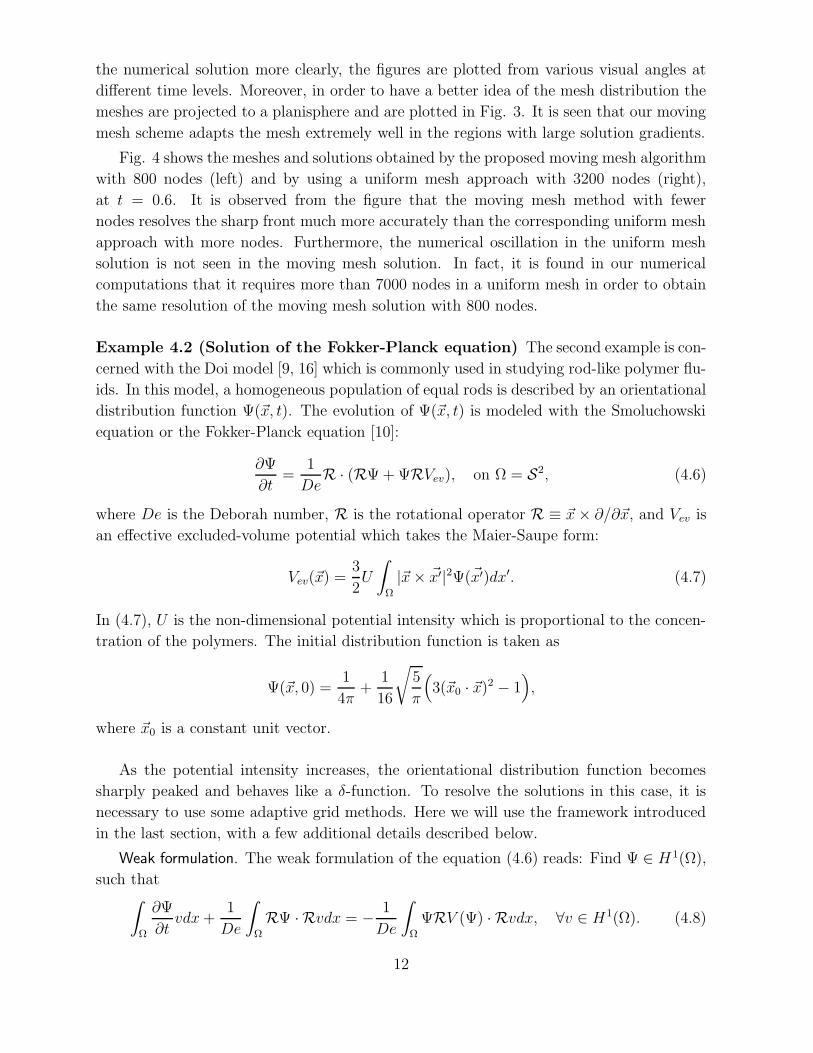
Fig. 4 shows the meshes and solutions obtained by the proposed moving mesh algorithm

with 800 nodes (left) and by using a uniform mesh approach with 3200 nodes (right),

at t = 0.6. It is observed from the figure that the moving mesh method with fewer

nodes resolves the sharp front much more accurately than the corresponding uniform mesh

approach with more nodes. Furthermore, the numerical oscillation in the uniform mesh

solution is not seen in the moving mesh solution. In fact, it is found in our numerical

computations that it requires more than 7000 nodes in a uniform mesh in order to obtain

the same resolution of the moving mesh solution with 800 nodes.

Example 4.2 (Solution of the Fokker-Planck equation) The second example is con-

cerned with the Doi model [9, 16] which is commonly used in studying rod-like polymer flu-

ids. In this model, a homogeneous population of equal rods is described by an orientational

distribution function Ψ(~x, t). The evolution of Ψ(~x, t) is modeled with the Smoluchowski

equation or the Fokker-Planck equation [10]:

∂Ψ

∂t=

1

DeR · (RΨ + ΨRVev), on Ω = S2, (4.6)

where De is the Deborah number, R is the rotational operator R ≡ ~x × ∂/∂~x, and Vev is

an effective excluded-volume potential which takes the Maier-Saupe form:

Vev(~x) =3

2U

∫

Ω

|~x× ~x′|2Ψ(~x′)dx′. (4.7)

In (4.7), U is the non-dimensional potential intensity which is proportional to the concen-

tration of the polymers. The initial distribution function is taken as

Ψ(~x, 0) =1

4π+

1

16

√

5

π

(

3(~x0 · ~x)2 − 1)

,

where ~x0 is a constant unit vector.

As the potential intensity increases, the orientational distribution function becomes

sharply peaked and behaves like a δ-function. To resolve the solutions in this case, it is

necessary to use some adaptive grid methods. Here we will use the framework introduced

in the last section, with a few additional details described below.

Weak formulation. The weak formulation of the equation (4.6) reads: Find Ψ ∈ H 1(Ω),

such that∫

Ω

∂Ψ

∂tvdx +

1

De

∫

Ω

RΨ · Rvdx = − 1

De

∫

Ω

ΨRV (Ψ) · Rvdx, ∀v ∈ H1(Ω). (4.8)

12

XY

Z

X

Z

Y

X

Z

Y X Y

Z

X Y

Z

X Y

Z

Figure 2: Example 4.1. The adaptive meshes on a sphere with 800 nodes from t = 0 to t = 1.5.

13

Figure 3: Example 4.1. The adaptive meshes on planisphere using 800 nodes from t = 0 to

t = 1.5.

In the finite element space Hh, the above weak form can be approximated as: Find Ψh ∈ Hh,

such that

∫

Ω

∂Ψh

∂tvhdx +

1

De

∫

Ω

RΨh · Rvhdx = − 1

De

∫

Ω

ΨhRV (Ψh) · Rvhdx, ∀vh ∈ Hh(Ω). (4.9)

For the temporal approximation, similar to [7] we use a semi-implicit three-step Runge-

Kutta scheme to solve (4.9): Find Ψn+1h ∈ Hh, such that

• Step 1:

∫

Ω

Ψ(1)h − Ψn

h

4t/3vhdx +

1

De

∫

Ω

RΨ(1)h · Rvhdx

= − 1

De

∫

Ω

ΨnhRV (Ψn

h) · Rvhdx, ∀vh ∈ Hh .

(4.10)

14

X

Z

Y X

Z

Y

Figure 4: Example 4.1. The adaptive mesh on sphere with 800 nodes (left) and uniform mesh

with 3200 nodes (right) at t = 0.6.

• Step 2:

∫

Ω

Ψ(2)h − Ψn

h

4t/2vhdx +

1

De

∫

Ω

RΨ(2)h · Rvhdx

= − 1

De

∫

Ω

Ψ(1)h RV (Ψ

(1)h ) · Rvhdx, ∀vh ∈ Hh,

(4.11)

• Step 3:∫

Ω

Ψn+1h − Ψn

h

4tvhdx +

1

De

∫

Ω

RΨn+1h · Rvhdx

= − 1

De

∫

Ω

Ψ(2)h RV (Ψ

(2)h ) · Rvhdx, ∀vh ∈ Hh,

(4.12)

Note that in each step above the diffusion term is treated implicitly while the nonlinear

term is treated explicitly. With this treatment, a standard stability criterion of CFL-type

applies; and in our computations a uniform time step is used. By doing this, it is well

known that the moving mesh method does not gain much in time-stepping, since the time

steps are controlled by the smallest size of the finite elements. One possible way of further

speed-up in temporal discretization is to use the local time stepping technique, see, e.g.,

[28].

Monitor functions. For a piecewise linear approximation φh to a function φ, the following

formula is adopted to approximate the computational error:

|φ− φh|1,Ω ∼√

∑

l : interior edge

∫

l

[

Rφh · ~tl]2

dl, (4.13)

where ~tl is the unit tangential vector of the edge l and [·] is the jump along the edge l;

see, e.g., [7, 19]. With this a posteriori interpolant error estimator, a monitor function is

15

Time

S

0 0.005 0.01 0.015 0.02 0.0250.3

0.4

0.5

0.6

0.7

0.8

0.9

1

1.1

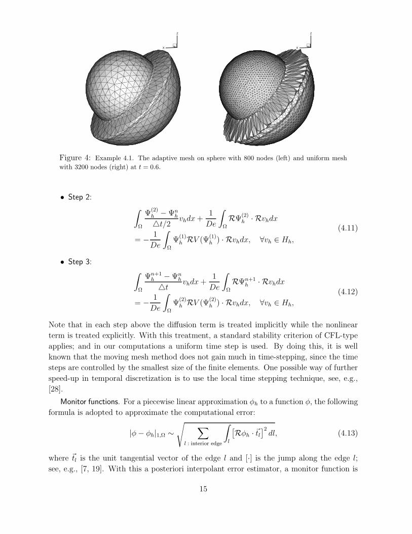
Figure 5: Example 4.2. Evolution of the scalar order parameter S with U = 1000.

proposed as

m(Ψh)|K =1

|K|∑

l⊂∂K

|l|∫

l

[

RΨh · ~tl]2

dl , ∀K ∈ Th . (4.14)

The instantaneous average molecular orientation is quantified by the order parameter tensor

S = 〈xx〉 − 1

3I. (4.15)

The scalar order parameter S = 32λ represents the degree of molecular alignment, where

λ is the eigenvalue with the largest absolute value for S. It lies in the range 0 ∼ 1 with

S = 0 for an isotropic phase, and S = 1 for rods that are all aligned in the same direction.

Fig. 5 shows the evolution of the scalar order parameter S with U = 100. In this case,

the stationary scalar order parameter S is very close to 1, indicating that all the molecular

directions converge to one direction and the distribution function is very singular.

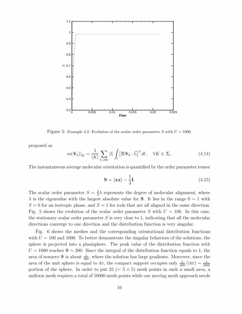
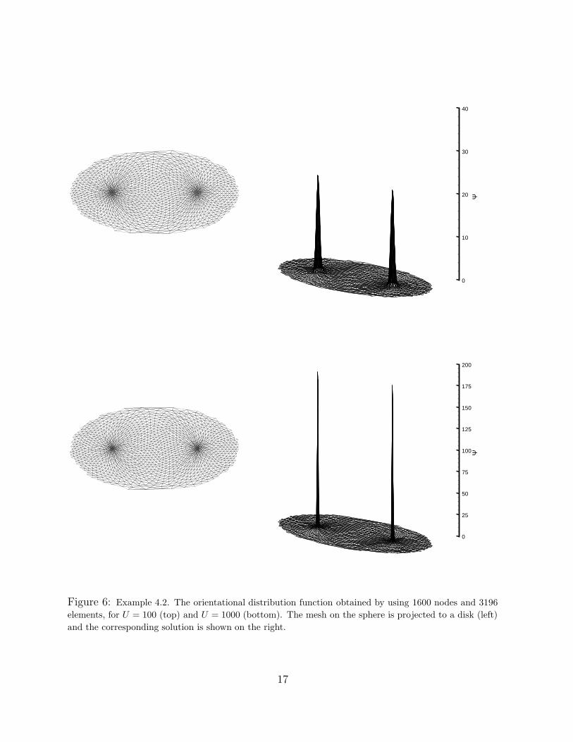
Fig. 6 shows the meshes and the corresponding orientational distribution functions

with U = 100 and 1000. To better demonstrate the singular behaviors of the solutions, the

sphere is projected into a planisphere. The peak value of the distribution function with

U = 1000 reaches Ψ ∼ 200. Since the integral of the distribution function equals to 1, the

area of nonzero Ψ is about 1200

, where the solution has large gradients. Moreover, since the

area of the unit sphere is equal to 4π, the compact support occupies only 1200

/(4π) ∼ 12000

portion of the sphere. In order to put 25 (= 5 × 5) mesh points in such a small area, a

uniform mesh requires a total of 50000 mesh points while our moving mesh approach needs

16

0

10

20

30

40

Ψ

0

25

50

75

100

125

150

175

200

Ψ

Figure 6: Example 4.2. The orientational distribution function obtained by using 1600 nodes and 3196

elements, for U = 100 (top) and U = 1000 (bottom). The mesh on the sphere is projected to a disk (left)

and the corresponding solution is shown on the right.

17

-3 -2 -1 0 1 2 3

0.5

1

1.5

2

2.5

3

3.5

4

4.5

5

5.5

6

1 1.5 2

1

1.5

2

Figure 7: Example 4.2. The close-up of the adaptive mesh for U = 1000 (bottom figure of Fig. 6).

1600 points only. By a close-up look of the mesh structure in Fig. 7, it is seen that with

the moving mesh approach more grid points are pushed into the (small) blow-up region.

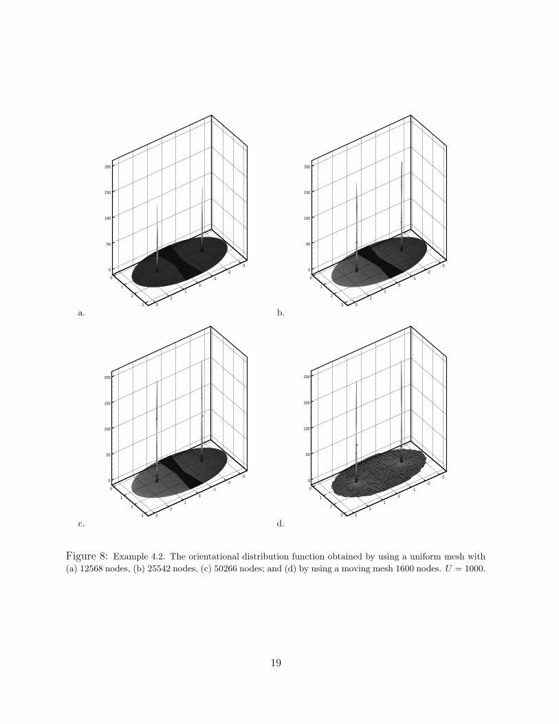
More comparisons are made for Example 4.2 with U = 1000. In Fig. 8, we compare the

numerical solutions obtained by using the uniform mesh (nodes 12568, 25542 and 50266,

respectively) and by using the adaptive moving mesh (1600 nodes). It is seen that the

moving mesh solution with 1600 nodes is more accurate than the uniform mesh solution

with 25542 nodes, and is comparable to the uniform mesh solution with 50266 nodes. This

is consistent with our estimate above quite well. Finally, it is necessary to compare the

total CPU time usage for these computations. Table 1 gives the relevant CPU time usages

with various numbers of nodes. The time step used is ∆t = 10−6 and the total time is

T = 2× 10−3. For this particular computation, the memory savings with the moving mesh

18

a.

0

50

100

150

200

-3

-2

-1

0

1

2

3

0

1

2

3

b.

0

50

100

150

200

-3

-2

-1

0

1

2

3

0

1

2

3

c.

0

50

100

150

200

-3

-2

-1

0

1

2

3

0

1

2

3

d.

0

50

100

150

200

-3

-2

-1

0

1

2

3

0

1

2

3

Figure 8: Example 4.2. The orientational distribution function obtained by using a uniform mesh with

(a) 12568 nodes, (b) 25542 nodes, (c) 50266 nodes; and (d) by using a moving mesh 1600 nodes. U = 1000.

19

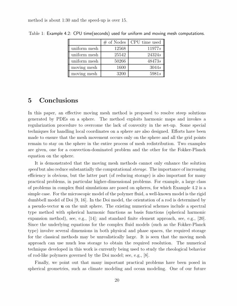
method is about 1:30 and the speed-up is over 15.

Table 1: Example 4.2: CPU time(seconds) used for uniform and moving mesh computations.

# of Nodes CPU time used

uniform mesh 12568 11977s

uniform mesh 25542 24324s

uniform mesh 50266 48473s

moving mesh 1600 3044s

moving mesh 3200 5981s

5 Conclusions

In this paper, an effective moving mesh method is proposed to resolve steep solutions

generated by PDEs on a sphere. The method exploits harmonic maps and invokes a

regularization procedure to overcome the lack of convexity in the set-up. Some special

techniques for handling local coordinates on a sphere are also designed. Efforts have been

made to ensure that the mesh movement occurs only on the sphere and all the grid points

remain to stay on the sphere in the entire process of mesh redistribution. Two examples

are given, one for a convection-dominated problem and the other for the Fokker-Planck

equation on the sphere.

It is demonstrated that the moving mesh methods cannot only enhance the solution

speed but also reduce substantially the computational storage. The importance of increasing

efficiency is obvious, but the latter part (of reducing storage) is also important for many

practical problems, in particular higher-dimensional problems. For example, a large class

of problems in complex fluid simulations are posed on spheres, for which Example 4.2 is a

simple case. For the microscopic model of the polymer fluid, a well-known model is the rigid

dumbbell model of Doi [9, 16]. In the Doi model, the orientation of a rod is determined by

a pseudo-vector u on the unit sphere. The existing numerical schemes include a spectral

type method with spherical harmonic functions as basis functions (spherical harmonic

expansion method), see, e.g., [14]; and standard finite element approach, see, e.g., [20].

Since the underlying equations for the complex fluid models (such as the Fokker-Planck

type) involve several dimensions in both physical and phase spaces, the required storage

for the classical methods may be unrealistically large. It is seen that the moving mesh

approach can use much less storage to obtain the required resolution. The numerical

technique developed in this work is currently being used to study the rheological behavior

of rod-like polymers governed by the Doi model; see, e.g., [8].

Finally, we point out that many important practical problems have been posed in

spherical geometries, such as climate modeling and ocean modeling. One of our future

20

projects is to extend the numerical techniques developed in this work to solve some practical

problems defined on spheres with solution singularity.

Acknowledgments

The research of Di and Li was supported in part by the Joint Applied Mathematics Research

Institute between Peking University and Hong Kong Baptist University. The research

of Tang was supported by CERG Grants of Hong Kong Research Grant Council, FRG

grants of Hong Kong Baptist University, and NSAF Grant #10476032 of National Science

Foundation of China. The research of Zhang is partially supported by the special funds

for Major State Research Projects 2005CB1704 and National Science Foundation of China

for Distinguished Young Scholars 10225103.

References

[1] A. Anderson, X. Zheng, and V. Cristini, Adaptive unstructured volume remeshing - i:

The method, J. Comput. Phys. 208 (2005), 616–625.

[2] B.N. Azarenok and T. Tang, Second-order Godunov-type scheme for reactive flow

calculations on moving meshes, J. Comput. Phys. 106 (2005), 48–80.

[3] M.J. Baines, M.E. Hubbard, and P.K. Jimack, A moving mesh finite element algorithm

for the adaptive solution of time-dependent partial differential equations with moving

boundaries, Appl. Numer. Math. 54 (2005), 450–469.

[4] G. Beckett, J. A. Mackenzie, and M. L. Robertson, A moving mesh finite element

method for the solution of two-dimensional Stephan problems, J. Comput. Phys. 168

(2001), 500–518.

[5] W.M. Cao, W.Z. Huang, and R.D. Russell, An r-adaptive finite element method based

upon moving mesh PDEs, J. Comput. Phys. 149 (1999), 221–244.

[6] , A study of monitor functions for two-dimensional adaptive mesh generation,

SIAM J. Sci. Comput. 20 (1999), 1978–1994.

[7] Y. Di, R. Li, T. Tang, and P.W. Zhang, Moving mesh finite element methods for the

incompressible Navier-Stokes equations, SIAM J. Sci. Comput. 26 (2005), 1036–1056.

[8] Y. Di and P.W. Zhang, The shear kinetic analysis for nematic polymers with high

potential intensities, Commun. Comput. Phys. (2006).

21

[9] M. Doi, Molecular dynamics and rheolgical properties of concentrated solutions of rod-

like polymers in isotropic and liquid crystalline phases, J. Polym. Sci. 19 (1981), 229–

243.

[10] M. Doi and S.F. Edwards, The Theory of Polymer Dynamics, Oxford University Press,

1986.

[11] Q. Du and M. Gunzburger, Grid generation and optimization based on centroidal

Voronoi tessellations, Appl. Math. Comput. 113 (2002), 591–607.

[12] A.S. Dvinsky, Adaptive grid generation from harmonic maps on Riemannian mani-

folds, J. Comput. Phys. 95 (1991), 450–476.

[13] J. Eell and J.H. Sampson, Harmonic mapping of Riemannian manifolds, Amer. J.

Math. 86 (1964), 109–160.

[14] M. G. Forest, Q. Wang, and R. Zhou, The flow-phase diagram of Doi-Hess theory for

sheared nematic polymers II: finite shear rates, Rheological Acta 44 (2004), 80–95.

[15] R. Hamilton, Harmonic Maps of Manifolds with Boundary, vol. 471, Springer-Verlag,

New York, 1975.

[16] S.Z. Hess, Fokker-Planck-equation approach to flow alignment in liquid crystals, Z.

Naturforsch. A 31A (1976), 1034–1037.

[17] W. Huang and W. Sun, Variational mesh adaptation II: Error estimates and monitor

functions, J. Comput. Phys. 184 (2003), 619–648.

[18] W.Z. Huang, Mathematical principles of anisotropic mesh adaptation, Commun. Com-

put. Phys. 1 (2006), 276–310.

[19] R. Li, W.-B. Liu, H.-P. Ma, and T. Tang, Adaptive finite element approximation

for distributed elliptic optimal control problems, SIAM J. Control Optim. 41 (2002),

1321–1349.

[20] R. Li, C. Luo, and P.-W. Zhang, Numerical simulation of Doi model of polymeric

fluids, Adv. in Sci. Comput. & Appl. (Y. Lu, W. Sun, and T. Tang, eds.), 2004,

pp. 258–273.

[21] R. Li, T. Tang, and P.-W. Zhang, Moving mesh methods in multiple dimensions based

on harmonic maps, J. Comput. Phys. 170 (2001), 562–588.

[22] , A moving mesh finite element algorithm for singular problems in two and

three space dimensions, J. Comput. Phys. 177 (2002), 365–393.

[23] G. Liao, F. Liu, G. D. Pena, D. Peng, and S. Osher, Level-set-based deformation

methods for adaptive grids, J. Comput. Phys. 159 (2000), 103–122.

22

[24] K. Lipnikov and M. Shashkov, The error-minimization-based strategy for moving mesh

methods, Commun. Comput. Phys. 1 (2006), 53–80.

[25] R.S. Palais, Foundations of Global Nonlinear Analysis, Benjamin, New York, 1968.

[26] J. Sacks and K. Uhlenbeck, The existence of minimal immersions of 2-spheres, Ann.

Math. 113 (1981), 1–24.

[27] R. Schoen and S.-T. Yau, On univalent harmonic maps between surfaces, Invent. Math.

44 (1978), 265–278.

[28] Z.-J. Tan, Z.-R. Zhang, Y.-Q. Huang, and T. Tang, Moving mesh methods with locally

varying time steps, J. Comput. Phys. 200 (2004), 347–367.

[29] H.-Z. Tang, A moving mesh method for the euler flow calculations using a directional

monitor function, Commun. Comput. Phys. 1 (2006).

[30] H.Z. Tang and T. Tang, Adaptive mesh methods for one- and two-dimensional hyper-

bolic conservation laws, SIAM J. Numer. Anal. 41 (2003), 487–515.

[31] M.A. Walkley, P.H. Jimack, P.K. Kelmanson, and J.L. Summers, Finite element sim-

ulation of three-dimensional free-surface flow problems, J. Sci. Comput. 24 (2005),

147–162.

[32] D.S. Wang and X.P. Wang, A three-dimensional adaptive method based on the iterative

grid redistribution, J. Comput. Phys. 199 (2004), 423–426.

[33] A. Winslow, Numerical solution of the quasi-linear Poisson equation, J. Comput. Phys.

1 (1967), 149–172.

[34] P. A. Zegeling, On resistive mhd models with adaptive moving meshes, J. Sci. Comput.

24 (2005), 263–284.

23