Moving Big Data to The Cloud:An Online Cost-Minimizing Approach

Linquan Zhang, Chuan Wu, Zongpeng Li, Chuanxiong Guo, Minghua Chen and Francis C.M. Lau

Abstract—Cloud computing, rapidly emerging as a new com-putation paradigm, provides agile and scalable resource accessin a utility-like fashion, especially for the processing of big data.An important open issue here is to efficiently move the data,from different geographical locations over time, into a cloud foreffective processing. The de facto approach of hard drive shippingis not flexible or secure. This work studies timely, cost-minimizingupload of massive, dynamically-generated, geo-dispersed datainto the cloud, for processing using a MapReduce-like framework.Targeting at a cloud encompassing disparate data centers, wemodel a cost-minimizing data migration problem, and proposetwo online algorithms: an online lazy migration (OLM) algorithmand a randomized fixed horizon control (RFHC) algorithm , foroptimizing at any given time the choice of the data center for dataaggregation and processing, as well as the routes for transmittingdata there. Careful comparisons among these online and offlinealgorithms in realistic settings are conducted through extensiveexperiments, which demonstrate close-to-offline-optimum perfor-mance of the online algorithms.

Index Terms—Cloud Computing, Big Data, Online Algorithms

I. INTRODUCTION

The cloud computing paradigm enables rapid on-demandprovisioning of server resources (CPU, storage, bandwidth)to users, with minimal management efforts. Recent cloudplatforms, as exemplified by Amazon EC2 and S3, MicrosoftAzure, Google App Engine, Rackspace [1], etc., organize ashared pool of servers from multiple data centers, and servetheir users using virtualization technologies.

The elastic and on-demand nature of resource provisioningmakes a cloud platform attractive for the execution of var-ious applications, especially computation-intensive ones [2],[3]. More and more data-intensive Internet applications, e.g.,Facebook, Twitter, and big data analytics applications, suchas the Human Genome Project [4], are relying on the cloudsfor processing and analyzing their petabyte-scale data sets,with a computing framework such as MapReduce and Hadoop[5], [6]. For example, Facebook-like social media sites collect

Manuscript received on December 1, 2012; revised on May 28, 2012. Somepreliminary results were presented at IEEE INFOCOM 2013, mini-conference,Turin, Italy, April, 2013.

L. Zhang and Z. Li are with the Department of Computer Science,University of Calgary. Email: linqzhan, zongpeng@ucalgary.ca. C. Wuand F. C.M. Lau are with the Department of Computer Science, TheUniversity of Hong Kong. Email: cwu, fcmlau@cs.hku.hk. C. Guo is withMicrosoft. Email: chguo@microsoft.com. M. Chen is with the Departmentof Information Engineering, The Chinese University of Hong Kong. Email:minghua@ie.cuhk.edu.hk.

Work supported by NSERC, Canada (RT733206), RGC, Hong Kong(717812, AoE/E-02/08, 411010, 411011), and National Basic Research Pro-gram of China (2012CB315904, 2013CB336700)

their Web server logs, Internet click data, social activityreports, etc., from various locations over time, and parsethem using Mapreduce/Hadoop to uncover usage patterns andhidden correlations, in order to facilitate marketing decisions.

While most efforts have been devoted to designing bettercomputing models for big data analytics, an important issuehas largely been left out in this respect: How does one movethe massive amounts of data into a cloud, in the very firstplace? The current practice is to copy the data into largehard drives for physically transportation to the data center[7], [8], or even to move entire machines [9]. Such physicaltransportation incurs undesirable delay and possible servicedowntime, while outputs of the data analysis are often neededto be presented to users in the most timely fashion [9]. It is alsoless secure, given that the hard drives are prone to infectionof malicious programs and damages from road accidents. Asafer and more flexible data migration strategy is in need, tominimize any potential service downtime.

The challenge escalates when we target at dynamicallyand continuously produced data from different geographicallocations, e.g., astronomical data from disparate observato-ries [10], usage data from different Facebook Web servers.With dynamic data, an efficient online algorithm is desired,for timely guiding the transfer of data into the cloud overtime. For geo-dispersed data sets, we wish to select the bestdata center to aggregate all data onto, for processing with aMapReduce-like framework, which is efficient to process datawithin one data center but not across data centers, due to theenormous overhead of inter-data center data moving in thestage of shuffle and reduce [11]. For example, Amazon ElasticMapReduce launches all processing nodes of a MapReduce jobin the same EC2 Availability Zone [12].

As the first dedicated effort in the cloud computing lit-erature, this work studies timely, cost-minimizing migrationof massive amounts of dynamically-generated, geo-disperseddata into the cloud, for processing using a MapReduce-likeframework. Targeting a typical cloud platform that encom-passes disparate data centers of different resource charges, wecarefully model the cost-minimizing data migration problem,and propose efficient offline and online algorithms, whichoptimize the routes of data into the cloud and the choice of thedata center for data processing, at any give time. Our detailedcontributions are as follows:

We analyze the detailed cost composition and identify theperformance bottleneck for moving data into the cloud, andformulate an offline optimal data migration problem. Theoptimization computes optimal data routing and aggregation

strategies at any given time, and minimizes the overall systemcost and data transfer delay, over a long run of the system. We propose a polynomial-time dynamic programming basedalgorithm to solve the offline optimal data migration problem,given complete knowledge of data generation in the temporaldomain. The derived offline optimal strategies serve as abenchmark for our online algorithms. Two efficient online algorithms are proposed to practicallyguide data migration over time: an online lazy migration(OLM) algorithm and a randomized fixed horizon control(RFHC) algorithm. Theoretical analyses show that the OLMalgorithm achieves a worst-case competitive ratio of 2.55,without the need of any future information and regardlessof the system scale, under the typical settings in real-worldscenarios. The RFHC algorithm achieves a competitive ratioof 1 + 1

l+1κλ that approaches 1 as the lookahead window l

grows. Here κ and λ are system dependent parameters ofsimilar magnitudes. We conduct extensive experiments to evaluate the per-formance of our online and offline algorithms, using real-world meteorological data generation traces. The online algo-rithms can achieve close-to-offline-optimum performance inmost cases examined, revealing that the theoretical worst-casecompetitive ratios are pessimistic, and only correspond to rarescenarios in practice.

In the rest of the paper, we discuss related work in Sec. II,describe the system and problem models in Sec. III, andpresent the offline and online solutions in Sec. IV and Sec. Vrespectively. Evaluation results are presented in Sec. VI.Sec. VII concludes the paper.

II. RELATED WORK

A series of recent work studies application migration tothe cloud. Hajjat et al. [13] develop an optimization modelfor migrating enterprise IT applications onto a hybrid cloud.Cheng et al. [14] and Wu et al. [15] advocate deployingsocial media applications into clouds, for leveraging the richresources and pay-as-you-go pricing. These projects focus onworkflow migration and application performance optimization,by carefully deciding the modules to be moved to the cloudand the data caching/replication strategies in the cloud. Thevery first question of how to move large volumes of applicationdata into the cloud is not explored.

Few existing work discussed such transfer of big data to thecloud. Cho et al. [16] design Pandora, a cost-aware planningsystem for data transfer to the cloud provider, via both theInternet and courier services. The same authors [17] laterpropose a solution to minimize the transfer latency under abudget constraint. Different from our study, they focus onstatic scenarios with a fixed amount of bulk data to transfer,rather than dynamically generated data; in addition, a singlecloud site is considered, while our study pays attention tomultiple data centers.

A number of online algorithms have been proposed toaddress different cloud computing and data center issues.For online algorithms without future information, Lin etal. [18] investigate energy-aware dynamic server provisioning,

by proposing a Lazy Capacity Provisioning algorithm witha 3-competitive ratio. Mathew et al. [19] tackle the energy-aware load balancing problem in the content delivery networks(CDNs) by an online Hibernate algorithm, which strikes abalance between energy consumption and customer service-level agreements (SLAs). However, no theoretical analysis onthe performance, in terms of competitive ratio, is provided.

For online algorithms assuming lookahead into the future,Lu and Chen [20] study the dynamic provisioning problemin data centers, and design future-aware algorithms based onthe classic ski-rental online algorithm, where the competitiveratios can be significantly improved by exploiting the looka-head information up to the break-even interval . Lin et al. [21]investigate load balancing among geographically-distributeddata centers, apply a receding horizon control (RHC) algo-rithm, and show that the competitive ratio can be reducedsubstantially by leveraging predicted future information, viarelaxing the optimization variables. Due to the unique integerrequirement on the decision variables, our problem cannotbe transformed into the ski-rental framework, nor relaxed toutilize the RHC framework. Our RFHC algorithm handles theinteger restriction via randomization instead.

This work fills gaps in the existing literature on the transferof large amounts of data to the cloud in the following threeaspects: 1, we focus on dynamically generated data rather thanstatic scenarios with a fixed amount of bulk data; 2, our studypays attention to a cloud with multiple geo-distributed datacenters, while existing work often focuses on a single cloudsite; 3, existing techniques used to handle online problems inthe cloud do not directly apply in our study, due to the uniquestructure of our data transfer problem.

III. THE DATA MIGRATION PROBLEM

A. System Model

We consider a cloud consisting of K geo-distributed datacenters in a set of regions K, where K = |K|. A cloud user(e.g., a global astronomical telescope application) continuouslyproduces large volumes of data at a set D of multiple ge-ographic locations (e.g., dispersed telescope sites). The userconnects to the data centers from different data generationlocations via virtual private networks (VPNs), with G VPNgateways at the user side and K VPN gateways each collocatedwith a data center. Let G denote the set of VPN gateways atthe user side, with G = |G|. An illustration of the system is inFig. 1. A private (the user’s) network inter-connects the datageneration locations and the VPN gateways at the user side.Such a model reflects typical connection approaches betweenusers and public clouds (e.g., AWS Direct Connect [22],Windows Azure Virtual Network [23]), where dedicated, pri-vate network connections are established between a user’spremise and the cloud, for enhanced security and reliability,and guaranteed inter-connection bandwidth.

Inter-data centre connections within a cloud are usuallydedicated high-bandwidth lines [24]. Within the user’s privatenetwork, the data transmission bandwidth between a datageneration location d ∈ D and a VPN gateway g ∈ G islarge as well. The bandwidth Ugi on a VPN link (g, i) from

Legend

Data Location 1

Data Location 2

DC 1

DC 2

DC 3

DC 4

Gateways at

the user side

Gateways at the

data center side Intranet links in cloud

Internet links

Intranet links at the user side

GW2'

GW1'GW1

GW2

GW3

GW4

GW3'

GW4'

Fig. 1. An illustration of the cloud system.

user side gateway g to data center i is limited, and constitutesthe bottleneck in the system.

B. Cost-minimizing Data Migration: Problem Formulation

Assume the system executes in a time-slotted fashion [15],[18], [19], with slot length τ . Fd(t) bytes of data are producedat location d in slot t, for upload to the cloud. ldg is the latencybetween data location d ∈ D and user side gateway g ∈ G,pgi is the delay along VPN link (g, i), and ηik is the latencybetween data centers i and k. These delays, which can beobtained by a simple command such as ping, are dictated bythe respective geographic distances.

A cloud user needs to decide (i) via which VPN connec-tions to upload its data to the cloud, and (ii) to which datacenter to aggregate data, for processing by a MapReduce-likeframework, such that the monetary charges incurred, as wellas the latency for the data to reach the aggregation point, arejointly minimized. The total cost C to be minimized has fourcomponents: bandwidth cost, aggregate storage and computingcost, migration cost, and routing cost.Decision variables. Two types of optimization variables areformulated:(1) Data routing variable xd,g,i,k(t), ∀d ∈ D,∀g ∈ G, ∀i ∈K, ∀k ∈ K, denotes the portion of data Fd(t) produced atlocation d in t, to be uploaded through VPN connection(g, i) and then migrated to data center k for processing.xd,g,i,k(t) > 0 indicates that the data routing path d →g → i → k is employed, and xd,g,i,k = 0 otherwise. Letx = (xd,g,i,k(t))∀d∈D,∀g∈G,∀i∈K,∀k∈K, the set of feasible datarouting variables are:

X =

x(t) |

∑g∈G,i∈K,k∈K

xd,g,i,k(t) = 1 and xd,g,i,k ∈ [0, 1],

∀d ∈ D, ∀g ∈ G,∀i ∈ K, ∀k ∈ K. (1)

Here∑

g∈G,i∈K,k∈K xd,g,i,k(t) = 1 ensures that all dataproduced from location d are uploaded into the cloud in t.(2) Binary variable yk(t), ∀k ∈ K, indicates whether datacenter k is target of data aggregation in time slot t (yk(t) = 1)or not (yk(t) = 0). Following the practical requirement ofthe current MapReduce framework, we require that at anygiven time, exactly one data center is chosen. Let y(t) =(yk(t))∀k∈K, the set of possible data aggregation variables are:

Y =

y(t) |

∑k∈K

yk(t) = 1 and yk(t) ∈ 0, 1, ∀k ∈ K. (2)

Costs. The costs incurred in time slot t, for uploading the datainto the cloud and for processing the data at the selected datacenter, include the following components.(1) The overall bandwidth cost for uploading data via theVPN connections, where

∑d∈D,k∈K

Fd(t)xd,g,i,k(t) is the amount

uploaded via (g, i), and fgi is the charge for uploading onebyte of data via (g, i), derived from bandwidth prices set bythe cloud provider:

CBW (x(t)) ,∑

g∈G,i∈K

(fgi∑

d∈D,k∈K

Fd(t)xd,g,i,k(t)). (3)

(2) Storage and computation costs are important factors to con-sider in choosing the data aggregation point. In a large-scaleonline application, processing and analyzing in t may involvedata produced not only in t, but also from the past, in the formof raw data or intermediate processing results. For example,data analytics in social networks may re-run the data parsingflow when new data arrives, together using the new data andold data (or previous parsing results of the old data) [25].Without loss of generality, let the amount of current and his-tory data to process in t be F(t) =

∑tν=1(αν

∑d∈D Fd(ν)),

where∑

d∈D Fd(ν) is the total amount of data producedin time slot ν from different data generation locations, andweight αν ∈ [0, 1] is smaller for older times ν and αt = 1for the current time t. The value of αν is determined byspecific applications and can be obtained through statisticaldata. Assume all the other historical data, except those inF(t), are removed from the data centers where they wereprocessed, since all needed information has been stored inthe retained data. Let Ψk(F(t)) be a non-decreasing costfunction for storage and computation in data center k in t(e.g., Ψk(F(t)) = skF(t) + vkF(t), if sk and vk are theper-byte per-time-slot costs for storing and processing in datacenter k, respectively. The value of sk is determined by thecloud provider and the value of vk depends on both the cloudprovider and the specific application). The aggregate storageand computing cost incurred in the cloud in t is:

CDC(y(t)) ,∑k∈K

yk(t)Ψk(F(t)). (4)

(3) The best data center for data aggregation can differ in tthan in t − 1, due to temporal and spatial variations in datageneration. Historical data needed for processing together withnew data in t, at the amount of

∑t−1ν=1(αν

∑d∈D Fd(ν)), should

be moved from the earlier data center to the current, and amigration cost is incurred. Let ϕik(z) be the non-decreasingmigration cost to move z bytes of data from data center i todate center k, satisfying triangle inequality: ϕik(z) + ϕkj(z) ≥ϕij(z). ϕik(z) corresponds to upload/download bandwidthcharges for moving data out of/into a data center, and/orthe delay between the two data centers based on geographicdistance. The migration cost between t− 1 and t is:

CtMG(y(t), y(t− 1)) ,

∑i∈K

∑k∈K

([yi(t− 1)− yi(t)]+

[yk(t)− yk(t− 1)]+ϕik(

t−1∑ν=1

αν

∑d∈D

Fd(ν))).

(5)

Here [a − b]+ = maxa − b, 0. Since only one data center isselected for data processing in each time slot, there is at mostone non-zero term in the above summation, corresponding to

data centers i for t−1 and k (k = i) for t, [yi(t−1)−yi(t)]+ =

1 = [yk(t)− yk(t− 1)]+ = 1.(4) The latency incurred for data upload is an importantperformance measure, to be minimized in the data routing andaggregation process. Targeting both monetary cost minimiza-tion and delay minimization, we formulate a routing cost fordelays along the selected routing paths, and combine it withother costs to be the optimization objective. The overall routingcost in the system in t is:

CRT (x(t)) ,∑

d,g,i,k

Lxd,g,i,k(t)Fd(t)(ldg + pgi + ηik), (6)

where xd,g,i,k(t)Fd(t)(ldg + pgi + ηik) is the product of datavolume and delay along the routing path d → g → i → k.The weighted formula suggests that transferring a large volumeof data via a high latency path causes high cost. L is therouting cost weight converting xd,g,i,k(t)Fd(t)(ldg+pgi+ηik)into a monetary cost, reflecting how latency-sensitive the useris. A cloud user specifies L as a constant a priori. Latencyldg + pgi + ηik is fixed in each slot but can change over time.

In summary, the overall cost incurred in t in the system is:C(x(t), y(t)) =CBW (x(t)) + CDC(y(t))+

CtMG(y(t), y(t− 1)) + CRT (x(t)).

(7)

The offline optimization problem of minimizing the overallcost of data upload and processing over a time interval [1, T ]can be formulated as:

minimizeT∑

t=1

C(x(t), y(t)) (8)

subject to: ∀t = 1, . . . , T ,

(8a) x(t) ∈ X ,(8b)

∑d∈K,k∈K Fd(t)xd,g,i,k(t)/τ ≤ Ugi, ∀i ∈ K,∀g ∈ G,

(8c) xd,g,i,k(t) ≤ yk(t),∀d ∈ D, ∀g ∈ G, ∀i ∈ K, ∀k ∈ K,(8d) y(t) ∈ Y,

where C(x(t), y(t)), X , and Y are given in Eqn. (7), (1) and(2), respectively. Constraint (8b) states that the total amountof data routed via (g, i) into the cloud in each time slot shouldnot exceed the upload capacity of (g, i). (8c) ensures that arouting path d→g→i→k is used (xd,g,i,k(t) > 0), only if datacenter k is the point of data aggregation in t (yk(t) = 1).

An Online Algorithm takes input gradually as they becomeavailable, and computes output on the fly. An Offline Algorithmis given complete information into the future, and generates asolution once in its entirety [26]. Competitive ratio is widelyaccepted to measure the performance of online algorithms. Adeterministic minimizing online algorithm A is α-competitiveiff ∀I , A(I) ≤ α ·O(I), where I is a given sequence of input,A(I) is the total cost to complete I by A, O(I) denotes thecost to serve I by the optimal offline algorithm. Similarly, arandomized minimizing online algorithm A is α-competitiveiff ∀I , E(A(I)) ≤ α ·O(I).

IV. AN OPTIMAL OFFLINE ALGORITHM

We first present an offline algorithm, which derives thetheoretical minimum cost given complete knowledge of datageneration in both temporal and spatial domains. The offlinealgorithm solves (8) by computing the optimal data routing and

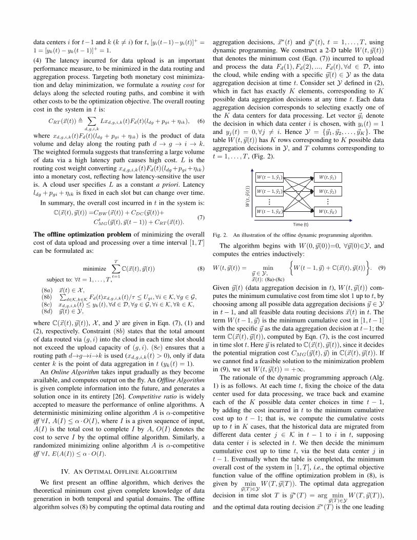
aggregation decisions, x∗(t) and y∗(t), t = 1, . . . , T , usingdynamic programming. We construct a 2-D table W (t, y(t))that denotes the minimum cost (Eqn. (7)) incurred to uploadand process the data Fd(1), Fd(2), ..., Fd(t), ∀d ∈ D, intothe cloud, while ending with a specific y(t) ∈ Y as the dataaggregation decision at time t. Consider set Y defined in (2),which in fact has exactly K elements, corresponding to Kpossible data aggregation decisions at any time t. Each dataaggregation decision corresponds to selecting exactly one ofthe K data centers for data processing. Let vector yi denotethe decision in which data center i is chosen, with yi(t) = 1and yj(t) = 0, ∀j = i. Hence Y = y1, y2, . . . , yK. Thetable W (t, y(t)) has K rows corresponding to K possible dataaggregation decisions in Y , and T columns corresponding tot = 1, . . . , T , (Fig. 2).

Time (t)

...

...

Fig. 2. An illustration of the offline dynamic programming algorithm.

The algorithm begins with W (0, y(0))=0, ∀y(0)∈Y , andcomputes the entries inductively:

W (t, y(t)) = miny ∈ Y,x(t): (8a)-(8c)

W (t− 1, y) + C(x(t), y(t))

. (9)

Given y(t) (data aggregation decision in t), W (t, y(t)) com-putes the minimum cumulative cost from time slot 1 up to t, bychoosing among all possible data aggregation decisions y ∈ Yin t− 1, and all feasible data routing decisions x(t) in t. Theterm W (t− 1, y) is the minimum cumulative cost in [1, t− 1]with the specific y as the data aggregation decision at t−1; theterm C(x(t), y(t)), computed by Eqn. (7), is the cost incurredin time slot t. Here y is related to C(x(t), y(t)), since it decidesthe potential migration cost CMG(y(t), y) in C(x(t), y(t)). Ifwe cannot find a feasible solution to the minimization problemin (9), we set W (t, y(t)) = +∞.

The rationale of the dynamic programming approach (Alg.1) is as follows. At each time t, fixing the choice of the datacenter used for data processing, we trace back and examineeach of the K possible data center choices in time t − 1,by adding the cost incurred in t to the minimum cumulativecost up to t − 1; that is, we compute the cumulative costsup to t in K cases, that the historical data are migrated fromdifferent data center j ∈ K in t − 1 to i in t, supposingdata center i is selected in t. We then decide the minimumcumulative cost up to time t, via the best data center j int − 1. Eventually when the table is completed, the minimumoverall cost of the system in [1, T ], i.e., the optimal objectivefunction value of the offline optimization problem in (8), isgiven by min

y(T )∈YW (T, y(T )). The optimal data aggregation

decision in time slot T is y∗(T ) = arg miny(T )∈Y

W (T, y(T )),

and the optimal data routing decision x∗(T ) is the one leading

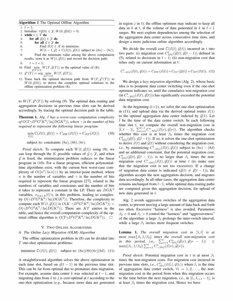
Algorithm 1 The Optimal Offline Algorithm1: t = 1;2: Initialize: ∀y(0) ∈ Y,W (0, y(0)) = 0;3: while t ≤ T do4: for all y(t) ∈ Y do5: for all y ∈ Y do6: Find x(t) ∈ X to minimize:7: W (t− 1, y) + C(x(t), y(t)) subject to (8a)− (8c);8: Find the minimum value among the above computation

results, store it as W (t, y(t)) and record the decision path;9: t = t+ 1;

10: Find miny(T )∈Y

W (T, y(T )) as the optimal value of (8);

11: y∗(T ) = arg miny(T )∈Y

W (T, y(T ));

12: Trace back the optimal decision path from W (T, y∗(T )) toW (0, y(0)), to derive the complete optimal solutions to theoffline optimization problem (8).

to W (T, y∗(T )) by solving (9). The optimal data routing andaggregation decisions in previous time slots can be derivedaccordingly, by tracing the optimal decision path in the table.

Theorem 1. Alg. 1 has a worst-case computation complexityof O(TγD3G3K8/ ln(DGK2)), where γ is the number of bitsrequired to represent the following linear program:

minx(t)

C(x(t), y(t)) = CBW (x(t)) + CRT (x(t)) (10)

subject to: constraints (8a), (8b), (8c).

Proof sketch: To compute each W (t, y(t)) using (9), wecan loop through the K possible values of y ∈ Y , and wheny is fixed, the minimization problem reduces to the linearprogram in (10). For a linear program, efficient polynomial-time algorithms exist, with the current best worst-case com-plexity of O([n3/ lnn]γ) by an interior-point method, wheren is the number of variables and γ is the number of bitsrequired to represent the linear program [27], related to thenumbers of variables and constraints and the number of bitsit takes to represent a constant in the LP. There are DGK2

variables, xd,g,i,k(t)’s, in this problem, leading to complex-ity O(γD3G3K6/ ln(DGK2)). Therefore, the complexity tocompute each W (t, y(t)) is O(K ·γD3G3K6/ ln(DGK2)) =O(γD3G3K7/ ln(DGK2)). There are KT entries in thetable, and hence the overall computation complexity of the op-timal offline algorithm is O(TγD3G3K8/ ln(DGK2)).

V. TWO ONLINE ALGORITHMS

A. The Online Lazy Migration (OLM) Algorithm

The offline optimization problem in (8) can be divided intoT one-shot optimization problems:

minimize C(x(t), y(t)) subject to: (8a)(8b)(8c)(8d). (11)

A straightforward algorithm solves the above optimization ineach time slot, based on y(t − 1) in the previous time slot.This can be far from optimal due to premature data migration.For example, assume data center k was selected at t− 1, andmigrating data from k to j is cost-optimal at t according to theone-shot optimization (e.g., because more data are generated

in region j in t); the offline optimum may indicate to keep alldata in k at t, if the volume of data generated in k in t + 1surges. We next explore dependencies among the selection ofthe aggregation data center across consecutive time slots, anddesign a more judicious online algorithm accordingly.

We divide the overall cost C(x(t), y(t)) incurred in t intotwo parts: (i) migration cost Ct

MG(y(t), y(t − 1)) defined in(5), related to decisions in t − 1; (ii) non-migration cost thatrelies only on current information at t:

Ct−MG(x(t), y(t)) = CBW (x(t))+CDC(y(t))+CRT (x(t)). (12)

We design a lazy migration algorithm (Alg. 2), whose basicidea is to postpone data center switching even if the one-shotoptimum indicates so, until the cumulative non-migration cost(in Ct

−MG(x(t), y(t))) has significantly exceeded the potentialdata migration cost.

At the beginning (t=1), we solve the one-shot optimizationin (11), and upload data via the derived optimal routes x(1)to the optimal aggregation data center indicted by y(1). Lett be the time of the data center switch. In each followingtime slot t, we compute the overall non-migration cost in[t, t − 1],

∑t−1ν=t

Cν−MG(x(ν), y(ν)). The algorithm checks

whether this cost is at least β2 times the migration costC t

MG(y(t), y(t−1)). If so, it solves the one-shot optimizationto derive x(t) and y(t) without considering the migration cost,i.e., by minimizing Ct

−MG(x(t), y(t)) subject to (8a) − (8d)and an additional constraint, that the potential migration cost,Ct

MG(y(t), y(t − 1)), is no larger than β1 times the non-migration cost Ct

−MG(x(t), y(t)) at time t (to make surethat the migration cost is not too excessive). If a changeof migration data center is indicated (y(t) = y(t − 1)), thealgorithm accepts the new aggregation decision, and migratesdata accordingly. In all other cases, the aggregation data centerremains unchanged from t−1, while optimal data routing pathsare computed given this aggregation decision, for upload ofnew data generated in t.

Alg. 2 avoids aggressive switches of the aggregation datacenter, to prevent moving a large amount of data back and forthtoo often. Excessive “laziness” is also avoided. Parametersβ2 > 0 and β1 > 0 control the “laziness” and “aggressiveness”of the algorithm: a large β2 prolongs the inter-switch interval,while a large β1 invites more frequent switches.

Lemma 1. The overall migration cost in [1, t] is atmost maxβ1,1/β2 times the overall non-migration costin this period, i.e.,

∑tν=1 C

νMG(y(ν), y(ν − 1)) ≤

maxβ1, 1/β2∑t

ν=1 Cν−MG(x(ν), y(ν)).

Proof sketch: Potential migration cost in t is at most β1

times the non-migration costs. For migration cost incurred inprevious time slots, i.e., C ti

MG(x(ti), y(ti)) where ti is the timeof aggregation data center switch, ∀i = 1, 2, · · · , the non-migration cost in the period from when this migration occursto the time before the next migration, i.e., in [ti, ti+1 − 1], isat least β2 times the migration cost. Hence we have

Algorithm 2 The Online Lazy Migration (OLM) Algorithm1: t = 1;2: t = 1; //Time slot when the last change of aggregation data

center happens3: Compute data routing decision x(1) and aggregation decision

y(1) by minimizing C(x(1), y(1)) subject to (8a)− (8d);4: Compute C1

MG(y(1), y(0)) and C1−MG(x(1), y(1));

5: while t ≤ T do6: if C t

MG(y(t), y(t−1)) ≤ 1β2

∑t−1

ν=tCν

−MG(x(ν), y(ν)) then7: Derive x(t) and y(t) by minimizing Ct

−MG(x(t), y(t)) in(12) subject to (8a)−(8d) and constraint Ct

MG(y(t), y(t−1)) ≤β1C

t−MG(x(t), y(t));

8: if y(t) = y(t− 1) then9: Use the new aggregation data center indicated by y(t);

10: t = t;11: if t < t then //not to use new aggregation data center12: y(t) = y(t − 1), compute data routing decision x(t) by

solving (10) if not derived;13: t = t+ 1;

t∑ν=1

CνMG(y(ν), y(ν − 1))

≤ 1/β2

t−1∑ν=1

Cν−MG(x(ν), y(ν)) + β1C

t−MG(x(t), y(t))

≤ maxβ1, 1/β2t∑

ν=1

Cν−MG(x(ν), y(ν)).

(13)

Lemma 2. The overall non-migration cost in [1, t] isat most ϵ times the total offline-optimal cost, i.e.,∑t

ν=1 Cν−MG(x(ν), y(ν)) ≤ ϵ

∑tν=1 C(x∗(ν), y∗(ν)), where

ϵ = maxν∈[1,T ]

maxy(ν)∈Y,x(ν):(8a)−(8c) Cν−MG(x(ν), y(ν))

miny(ν)∈Y,x(ν):(8a)−(8c) Cν−MG(x(ν), y(ν))

is the maximum ratio of the largest over the smallest possiblenon-migration cost incurred in a time slot, with different dataupload and aggregation decisions.

Proof sketch: By the definition of ϵ, at ν ∈ [1, t], thenon-migration cost of OLM is smaller than ϵ times the non-migration cost incurred by the optimal offline algorithm, i.e.,Cν

−MG(x(ν), y(ν)) ≤ ϵCν−MG(x

∗(ν), y∗(ν)). We havet∑

ν=1

Cν−MG(x(ν), y(ν))

≤ ϵt∑

ν=1

Cν−MG(x

∗(ν), y∗(ν))

≤ ϵ

t∑ν=1

Cν

−MG(x∗(ν), y∗(ν)) + Cν

MG(y∗(ν), y∗(ν − 1))

= ϵ

t∑ν=1

C(x∗(ν), y∗(ν)).

(14)

Theorem 2. The OLM Algorithm is ϵ(1 + maxβ1, 1/β2)-competitive.

Proof Sketch: The overall cost incurred by the OLMAlgorithm in [1, T ] is

∑Tν=1[C

νMG(y(ν), y(ν − 1)) +

Cν−MG(x(ν), y(ν))]. By Lemma 1 and Lemma 2:

T∑ν=1

[CνMG(y(ν), y(ν − 1)) + Cν

−MG(x(ν), y(ν))]

≤ (1 + maxβ1, 1/β2)T∑

ν=1

Cν−MG(x(ν), y(ν))

≤ ϵ(1 + maxβ1, 1/β2)T∑

ν=1

C(x∗(ν), y∗(ν)).

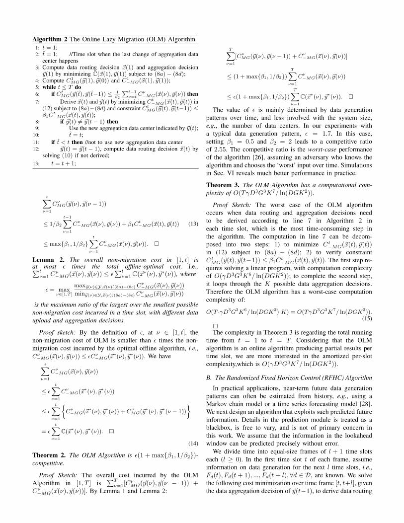
The value of ϵ is mainly determined by data generationpatterns over time, and less involved with the system size,e.g., the number of data centers. In our experiments witha typical data generation pattern, ϵ = 1.7. In this case,setting β1 = 0.5 and β2 = 2 leads to a competitive ratioof 2.55. The competitive ratio is the worst-case performanceof the algorithm [26], assuming an adversary who knows thealgorithm and chooses the ‘worst’ input over time. Simulationsin Sec. VI reveals much better performance in practice.

Theorem 3. The OLM Algorithm has a computational com-plexity of O(TγD3G3K7/ ln(DGK2)).

Proof Sketch: The worst case of the OLM algorithmoccurs when data routing and aggregation decisions needto be derived according to line 7 in Algorithm 2 ineach time slot, which is the most time-consuming step inthe algorithm. The computation in line 7 can be decom-posed into two steps: 1) to minimize Ct

−MG(x(t), y(t))in (12) subject to (8a) − (8d); 2) to verify constraintCt

MG(y(t), y(t−1)) ≤ β1Ct−MG(x(t), y(t)). The first step re-

quires solving a linear program, with computation complexityof O(γD3G3K6/ ln(DGK2)); to complete the second step,it loops through the K possible data aggregation decisions.Therefore the OLM algorithm has a worst-case computationcomplexity of:

O(T ·γD3G3K6/ ln(DGK2)·K) = O(TγD3G3K7/ ln(DGK2)).(15)

The complexity in Theorem 3 is regarding the total runningtime from t = 1 to t = T . Considering that the OLMalgorithm is an online algorithm producing partial results pertime slot, we are more interested in the amortized per-slotcomplexity,which is O(γD3G3K7/ ln(DGK2)).

B. The Randomized Fixed Horizon Control (RFHC) Algorithm

In practical applications, near-term future data generationpatterns can often be estimated from history, e.g., using aMarkov chain model or a time series forecasting model [28].We next design an algorithm that exploits such predicted futureinformation. Details in the prediction module is treated as ablackbox, is free to vary, and is not of primary concern inthis work. We assume that the information in the lookaheadwindow can be predicted precisely without error.

We divide time into equal-size frames of l + 1 time slotseach (l ≥ 0). In the first time slot t of each frame, assumeinformation on data generation for the next l time slots, i.e.,Fd(t), Fd(t + 1), ..., Fd(t + l),∀d ∈ D, are known. We solvethe following cost minimization over time frame [t, t+l], giventhe data aggregation decision of y(t−1), to derive data routing

Time

Fig. 3. An illustration of different FHC algorithms with l = 2.

Algorithm 3 The Randomized Fixed Horizon Control (RFHC)Algorithm

1: y(0) = 0;2: p = rand(1, l + 1); //A random integer within [1,l+1]3: if p = 1 then4: Derive x(1) · · · x(p − 1) and y(1) · · · y(p − 1) by solving

(16) over the time window [1, p− 1];5: t = p;6: while t ≤ T do7: if (t− p) mod (l + 1) = 0 then8: Derive x(t), · · · , x(t + l) and y(t), · · · , y(t + l) by

solving (16) over the time frame [t, t+ l];9: t = t+ 1;

decisions x(ν) and aggregation decisions y(ν), ∀ν = t, . . . , t+l, using Alg. 1 in Sec. IV:

minimizet+l∑ν=t

C(x(ν), y(ν)), (16)

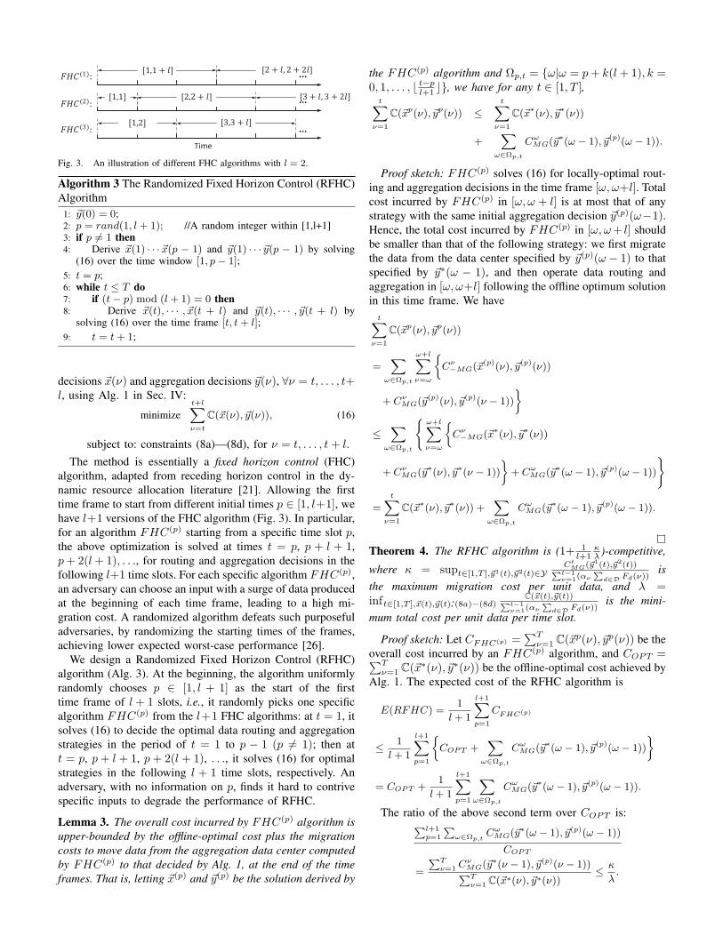
subject to: constraints (8a)—(8d), for ν = t, . . . , t+ l.The method is essentially a fixed horizon control (FHC)

algorithm, adapted from receding horizon control in the dy-namic resource allocation literature [21]. Allowing the firsttime frame to start from different initial times p ∈ [1, l+1], wehave l+1 versions of the FHC algorithm (Fig. 3). In particular,for an algorithm FHC(p) starting from a specific time slot p,the above optimization is solved at times t = p, p + l + 1,p+ 2(l+ 1), . . ., for routing and aggregation decisions in thefollowing l+1 time slots. For each specific algorithm FHC(p),an adversary can choose an input with a surge of data producedat the beginning of each time frame, leading to a high mi-gration cost. A randomized algorithm defeats such purposefuladversaries, by randomizing the starting times of the frames,achieving lower expected worst-case performance [26].

We design a Randomized Fixed Horizon Control (RFHC)algorithm (Alg. 3). At the beginning, the algorithm uniformlyrandomly chooses p ∈ [1, l + 1] as the start of the firsttime frame of l + 1 slots, i.e., it randomly picks one specificalgorithm FHC(p) from the l+1 FHC algorithms: at t = 1, itsolves (16) to decide the optimal data routing and aggregationstrategies in the period of t = 1 to p − 1 (p = 1); then att = p, p + l + 1, p + 2(l + 1), . . ., it solves (16) for optimalstrategies in the following l + 1 time slots, respectively. Anadversary, with no information on p, finds it hard to contrivespecific inputs to degrade the performance of RFHC.

Lemma 3. The overall cost incurred by FHC(p) algorithm isupper-bounded by the offline-optimal cost plus the migrationcosts to move data from the aggregation data center computedby FHC(p) to that decided by Alg. 1, at the end of the timeframes. That is, letting x(p) and y(p) be the solution derived by

the FHC(p) algorithm and Ωp,t = ω|ω = p+ k(l+ 1), k =0, 1, . . . , ⌊ t−p

l+1 ⌋, we have for any t ∈ [1, T ],t∑

ν=1

C(xp(ν), yp(ν)) ≤t∑

ν=1

C(x∗(ν), y∗(ν))

+∑

ω∈Ωp,t

CωMG(y

∗(ω − 1), y(p)(ω − 1)).

Proof sketch: FHC(p) solves (16) for locally-optimal rout-ing and aggregation decisions in the time frame [ω, ω+l]. Totalcost incurred by FHC(p) in [ω, ω + l] is at most that of anystrategy with the same initial aggregation decision y(p)(ω−1).Hence, the total cost incurred by FHC(p) in [ω, ω+ l] shouldbe smaller than that of the following strategy: we first migratethe data from the data center specified by y(p)(ω − 1) to thatspecified by y∗(ω − 1), and then operate data routing andaggregation in [ω, ω+l] following the offline optimum solutionin this time frame. We have

t∑ν=1

C(xp(ν), yp(ν))

=∑

ω∈Ωp,t

ω+l∑ν=ω

Cν

−MG(x(p)(ν), y(p)(ν))

+ CνMG(y

(p)(ν), y(p)(ν − 1))

≤

∑ω∈Ωp,t

ω+l∑ν=ω

Cν

−MG(x∗(ν), y∗(ν))

+ CνMG(y

∗(ν), y∗(ν − 1))

+ Cω

MG(y∗(ω − 1), y(p)(ω − 1))

=

t∑ν=1

C(x∗(ν), y∗(ν)) +∑

ω∈Ωp,t

CωMG(y

∗(ω − 1), y(p)(ω − 1)).

Theorem 4. The RFHC algorithm is (1+ 1l+1

κλ )-competitive,

where κ = supt∈[1,T ],y1(t),y2(t)∈YCt

MG(y1(t),y2(t))∑t−1ν=1(αν

∑d∈D Fd(ν))

isthe maximum migration cost per unit data, and λ =inft∈[1,T ],x(t),y(t):(8a)−(8d)

C(x(t),y(t))∑t−1ν=1(αν

∑d∈D Fd(ν))

is the mini-mum total cost per unit data per time slot.

Proof sketch: Let CFHC(p) =∑T

ν=1 C(xp(ν), yp(ν)) be theoverall cost incurred by an FHC(p) algorithm, and COPT =∑T

ν=1 C(x∗(ν), y∗(ν)) be the offline-optimal cost achieved byAlg. 1. The expected cost of the RFHC algorithm is

E(RFHC) =1

l + 1

l+1∑p=1

CFHC(p)

≤ 1

l + 1

l+1∑p=1

COPT +

∑ω∈Ωp,t

CωMG(y

∗(ω − 1), y(p)(ω − 1))

= COPT +1

l + 1

l+1∑p=1

∑ω∈Ωp,t

CωMG(y

∗(ω − 1), y(p)(ω − 1)).

The ratio of the above second term over COPT is:∑l+1p=1

∑ω∈Ωp,t

CωMG(y

∗(ω − 1), y(p)(ω − 1))

COPT

=

∑Tν=1 C

νMG(y

∗(ν − 1), y(p)(ν − 1))∑Tν=1 C(x∗(ν), y∗(ν))

≤ κ

λ.

Therefore, we conclude that: E(RFHC)COPT

≤ 1 + 1l+1

κλ .

Theorem 4 reveals that the more future steps predicted (thelarger l is), the closer the RFHC algorithm can approachthe offline optimal algorithm. Values of κ and λ are relatedto system input including prices and delays, and are lessinvolved with the data generation patterns and the number ofdata centers. In our experiments, κ

λ ≈ 0.69, and even withl = 1, the competitive ratio is already as low as 1.34. We alsoconducted experiments with imperfect predictions. Resultsshow that the performance remains good when accuracy isabove 80%. When l = 0, whether the RFHC algorithm orthe lazy migration algorithm performs better depends on thesystem input. We will evaluate their performance throughexperiments in the next section.

Theorem 5. The RFHC algorithm has a worst-case compu-tation complexity of

O(TγD3G3K7/ ln(DGK2)) if l = 0O(TγD3G3K8/ ln(DGK2)) if l > 0,

Proof sketch:Case 1: l = 0 (no lookahead). In this case, at time slot t,

the algorithm needs to go through the K possible aggregationdecisions of y ∈ Y to derive the one-shot optimum. For eachy, the linear program in (10) is solved, with a computationcomplexity of O(γD3G3K6/ ln(DGK2)). Hence, the RFHCalgorithm has a worst-case computation complexity of

O(T ·γD3G3K6/ ln(DGK2)·K) = O(TγD3G3K7/ ln(DGK2)).(17)

Case 2: l > 0. The algorithm computes the optimum of thedata migration problem over the equal-size frames using themethod introduced in Sec. IV. According to Theorem 1, theworst-case computation complexity of the RFHC algorithmin the first frame is O((p − 1)γD3G3K8/ ln(DGK2)), andO((l + 1)γD3G3K8/ ln(DGK2)) for each of the frames (ofl+1 slots) afterwards. Hence, the RFHC algorithm has a worst-case computation complexity of

O(⌊T − p

l + 1⌋ · (l + 1)γD3G3K8/ ln(DGK2))

+O((p− 1)γD3G3K8/ ln(DGK2))

= O(TγD3G3K8/ ln(DGK2)).

(18)

Theorem 5 shows the cumulative complexity from t = 1to t = T . Since RFHC is an online algorithm producingpartial results in each time frame, we are more interested inthe amortized per time frame complexity:

O(γD3G3K7/ ln(DGK2)) if l = 0O((l + 1)γD3G3K8/ ln(DGK2)) if l > 0,

(19)

VI. PERFORMANCE EVALUATION

A. Experiment Setup

Astronomical data processing usually involves Terabytes,Petabytes, or even Exabytes of data per day. Square KilometreArray (SKA) is an international project to build the world’slargest telescope distributed in Australia, New Zealand andSouth Africa. It is expected to produce a few Exabytes ofdata per day [29]. Such astronomical data from geo-distributedtelescopes is a natural target for our proposed algorithms.

We implement our offline and online algorithms on a clusterof 22 commodity computers (Intel(R) Pentium(R) D 3.0GHzwith dual cores, 1G RAM). We emulate a cloud of 8 datacenters in 8 regions (London, Bangalore, Hong Kong, Tokyo,San Francisco, Atlanta, Toronto and Sao Paulo), and a networkof 8 observatories scattered in 8 time zones (Canary Is-lands, South Africa, Urumqi, Western Australia, New Zealand,Hawaii, Arizona, and Middle Chile), producing Gigabytes ofastronomical data per night for upload into the cloud. Thereare 8 gateways collocated with the data centers and 6 user-sidegateways in Paris, Beijing, Sydney, Los Angeles, New Yorkand Rio de Janeiro, respectively. Each PC emulates one of userlocations, user-side gateways and data centers. Networkinginstead of computation is our focus of emulation. Each PCcan provide the ability to transfer a large amount of data viahigh-speed Ethernet. All 22 PCs are interconnected via a DellPowerConnect 5548 Switch. An additional PC is employed toperform the central controller to control the routing scheduleand the migration scheme within the cluster of 22 commoditycomputers. A typical cloud provider in practice usually hasup to 8 data centers (e.g., Amazon EC2 consists of 8 datacenters [30], Linode has 6 data centers [31] and DigitalOceanis operating 3 data centers [32].

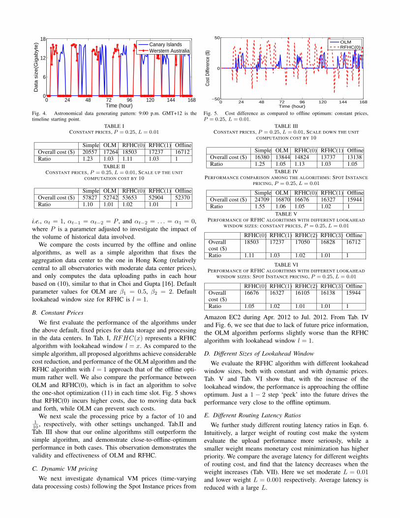
Since detailed astronomical data are not publicly available,synthetic traces are generated to drive our experiments. Weextract data generation patterns from a set of statistics on atmo-spheric visibility data collected at the Canarian observatories,from Feb. 2000 to Aug. 2003 [33]. Based on the strong cor-relation between the visibility and the quality of astronomicalimages [34], we produce astronomical data for each of the 8observatories following the extracted data generation pattern,but augment the volume to the Gigabyte scale. Fig. 4 depictsthe data patterns for two observatories, each producing databetween 9:00 p.m. to 5:00 a.m. in its local time.

Each time slot is set to one hour in our experiments.Link delays are set based on Round Trip Time (RTT) amongthe observatories, gateways and data centers, according togeographic distance: RTT (ms) = 0.02×Distance(km) + 5[35]. Bandwidths on the VPN connections are randomly drawnwithin [68, 100] Mbps. The unit charges of uploading data viathe VPN connections, fgi, are set within [0.10, 0.25] $/GB.The unit cost for storing and processing one GB of data,sk and vk in data center k, are set within [0.01, 0.1] $/hand [0.45, 0.55] $/h respectively, following typical charges inAmazon EC2 and S3 [30], [36] respectively, with small valuevariations. The rationale behind such setting of vk include: (i),TERAPIX [37], which is designed to handle large amounts ofastronomical data, can process 320 GB data per night, usinga cluster of 10 machines each configured with dual AthlonXP/MP 2400+ and 2 GB RAM; (ii), the measurement ofEC2 instances [30]. From (i) and (ii) we estimate the unitcost for processing 1 GB data, and the algorithm will setupenough number of VMs to execute MapReduce according tothe current data volume. The migration cost function, ϕik(z)is a linear function on the amount of data moved, z, with acost in the range of [0.10, 0.25] $/GB. The default value of Lto convert delay to cost is 0.01.

At time t, data produced in [t−2, t] are used for processing,

0 24 48 72 96 120 144 1680

6

12

18

Time (hour)

Data

siz

e(G

igabyt

e)

Canary IslandsWerstern Australia

Fig. 4. Astronomical data generating pattern: 9:00 p.m. GMT+12 is thetimeline starting point.

0 24 48 72 96 120 144 168−50

0

50

Time (hour)

Cos

t Diff

eren

ce ($

)

OLMRFHC(0)

Fig. 5. Cost difference as compared to offline optimum: constant prices,P = 0.25, L = 0.01.

TABLE ICONSTANT PRICES, P = 0.25, L = 0.01

Simple OLM RFHC(0) RFHC(1) OfflineOverall cost ($) 20557 17264 18503 17237 16712Ratio 1.23 1.03 1.11 1.03 1

TABLE IICONSTANT PRICES, P = 0.25, L = 0.01, SCALE UP THE UNIT

COMPUTATION COST BY 10

Simple OLM RFHC(0) RFHC(1) OfflineOverall cost ($) 57827 52742 53653 52904 52370Ratio 1.10 1.01 1.02 1.01 1

i.e., αt = 1, αt−1 = αt−2 = P , and αt−2 = . . . = α1 = 0,where P is a parameter adjusted to investigate the impact ofthe volume of historical data involved.

We compare the costs incurred by the offline and onlinealgorithms, as well as a simple algorithm that fixes theaggregation data center to the one in Hong Kong (relativelycentral to all observatories with moderate data center prices),and only computes the data uploading paths in each hourbased on (10), similar to that in Choi and Gupta [16]. Defaultparameter values for OLM are β1 = 0.5, β2 = 2. Defaultlookahead window size for RFHC is l = 1.

B. Constant Prices

We first evaluate the performance of the algorithms underthe above default, fixed prices for data storage and processingin the data centers. In Tab. I, RFHC(x) represents a RFHCalgorithm with lookahead window l = x. As compared to thesimple algorithm, all proposed algorithms achieve considerablecost reduction, and performance of the OLM algorithm and theRFHC algorithm with l = 1 approach that of the offline opti-mum rather well. We also compare the performance betweenOLM and RFHC(0), which is in fact an algorithm to solvethe one-shot optimization (11) in each time slot. Fig. 5 showsthat RFHC(0) incurs higher costs, due to moving data backand forth, while OLM can prevent such costs.

We next scale the processing price by a factor of 10 and110 , respectively, with other settings unchanged. Tab.II andTab. III show that our online algorithms still outperform thesimple algorithm, and demonstrate close-to-offline-optimumperformance in both cases. This observation demonstrates thevalidity and effectiveness of OLM and RFHC.

C. Dynamic VM pricing

We next investigate dynamical VM prices (time-varyingdata processing costs) following the Spot Instance prices from

TABLE IIICONSTANT PRICES, P = 0.25, L = 0.01, SCALE DOWN THE UNIT

COMPUTATION COST BY 10

Simple OLM RFHC(0) RFHC(1) OfflineOverall cost ($) 16380 13844 14824 13737 13138Ratio 1.25 1.05 1.13 1.03 1.05

TABLE IVPERFORMANCE COMPARISON AMONG THE ALGORITHMS: SPOT INSTANCE

PRICING, P = 0.25, L = 0.01

Simple OLM RFHC(0) RFHC(1) OfflineOverall cost ($) 24709 16870 16676 16327 15944Ratio 1.55 1.06 1.05 1.02 1

TABLE VPERFORMANCE OF RFHC ALGORITHMS WITH DIFFERENT LOOKAHEAD

WINDOW SIZES: CONSTANT PRICES, P = 0.25, L = 0.01

RFHC(0) RFHC(1) RFHC(2) RFHC(3) OfflineOverallcost ($)

18503 17237 17050 16828 16712

Ratio 1.11 1.03 1.02 1.01 1

TABLE VIPERFORMANCE OF RFHC ALGORITHMS WITH DIFFERENT LOOKAHEAD

WINDOW SIZES: SPOT INSTANCE PRICING, P = 0.25, L = 0.01

RFHC(0) RFHC(1) RFHC(2) RFHC(3) OfflineOverallcost ($)

16676 16327 16105 16138 15944

Ratio 1.05 1.02 1.01 1.01 1

Amazon EC2 during Apr. 2012 to Jul. 2012. From Tab. IVand Fig. 6, we see that due to lack of future price information,the OLM algorithm performs slightly worse than the RFHCalgorithm with lookahead window l = 1.

D. Different Sizes of Lookahead Window

We evaluate the RFHC algorithm with different lookaheadwindow sizes, both with constant and with dynamic prices.Tab. V and Tab. VI show that, with the increase of thelookahead window, the performance is approaching the offlineoptimum. Just a 1 − 2 step ‘peek’ into the future drives theperformance very close to the offline optimum.

E. Different Routing Latency Ratios

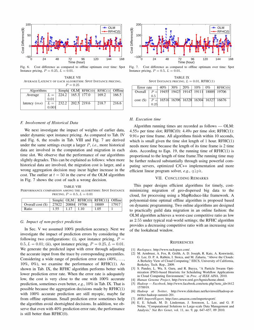
We further study different routing latency ratios in Eqn. 6.Intuitively, a larger weight of routing cost make the systemevaluate the upload performance more seriously, while asmaller weight means monetary cost minimization has higherpriority. We compare the average latency for different weightsof routing cost, and find that the latency decreases when theweight increases (Tab. VII). Here we set moderate L = 0.01and lower weight L = 0.001 respectively. Average latency isreduced with a large L.

0 24 48 72 96 120 144 168−50

0

50

100

Time (hour)

Cos

t Diff

eren

ce($

)

OLMRFHC(l)

Fig. 6. Cost difference as compared to offline optimum over time: SpotInstance pricing, P = 0.25, L = 0.01.

0 24 48 72 96 120 144 168−100

0

100

200

Time (hour)

Cos

t Diff

eren

ce($

)

OLMRFHC(l)

Fig. 7. Cost difference as compared to offline optimum over time: SpotInstance pricing, P = 0.5, L = 0.01.

TABLE VIIAVERAGE LATENCY OF EACH ALGORITHM: SPOT INSTANCE PRICING,

P = 0.25

Algorithms Simple OLM RFHC(0) RFHC(1) OfflineAverage L =

0.01224.2 165.3 177.0 169.2 166.5

latency (ms) L =0.001

232.2 202.5 219.6 218.7 216.6

F. Involvement of Historical Data

We next investigate the impact of weights of earlier data,under dynamic spot instance pricing. As compared to Tab. IVand Fig. 6, the results in Tab. VIII and Fig. 7 are derivedunder the same settings except a larger P , i.e., more historicaldata are involved in the computation and migration in eachtime slot. We observe that the performance of our algorithmsslightly degrades. This can be explained as follows: when morehistorical data are involved, the migration cost is larger, and awrong aggregation decision may incur higher increase in thecost. The outlier at t = 50 in the curve of the OLM algorithmin Fig. 7 shows the cost of such a wrong decision.

TABLE VIIIPERFORMANCE COMPARISON AMONG THE ALGORITHMS: SPOT INSTANCE

PRICING, P = 0.5, L = 0.01

Simple OLM RFHC(0) RFHC(1) OfflineOverall cost ($) 27822 20884 19706 18889 17917Ratio 1.55 1.17 1.10 1.05 1

G. Impact of non-perfect prediction

In Sec. V we assumed 100% prediction accuracy. Next weinvestigate the impact of prediction errors by considering thefollowing two configurations: (i), spot instance pricing, P =0.5, L = 0.01; (ii), spot instance pricing, P = 0.25, L = 0.01.We generate the predicted input with error through adjustingthe accurate input from the trace by corresponding percentiles.Considering a wide range of prediction error rates (40%, . . . ,10%, 0%), we examine the performance of RFHC(1). Asshown in Tab. IX, the RFHC algorithm performs better withlower prediction error rate. When the error rate is adequatelylow, the cost is very close to the one with 100% accurateprediction, sometimes even better, e.g., 10% in Tab. IX. That ispossible because the aggregation decisions made by RFHC(1)with 100% accurate prediction are still myopic, maybe farfrom offline optimum. Small prediction error sometimes helpthe algorithm avoid shortsighted decisions. In addition, we ob-serve that even with 40% prediction error rate, the performanceis still better than RFHC(0).

TABLE IXSPOT INSTANCE PRICING, L = 0.01, RFHC(1)

Error rate 40% 30% 20% 10% 0% RFHC(0)Overall P =

0.519455 19423 19147 19111 18889 19706

cost ($) P =0.25

16516 16396 16328 16304 16327 16676

H. Execution time

Algorithm running times are recorded as follows — OLM:4.55s per time slot; RFHC(0): 4.49s per time slot; RFHC(1):9.91s per time frame. All algorithms finish within 10 seconds,which is small given the time slot length of 1 hour. RFHC(1)needs more time because the length of its time frame is 2 timeslots. According to Eqn. 19, the running time of RFHC(1) isproportional to the length of time frame.The running time maybe further reduced substantially through using powerful com-puting servers, optimized C/C++ implementation and moreefficient linear program solver, e.g., glpk.

VII. CONCLUDING REMARKS

This paper designs efficient algorithms for timely, cost-minimizing migration of geo-dispersed big data to thecloud, for processing using a MapReduce-like framework. Apolynomial-time optimal offline algorithm is proposed basedon dynamic programming. Two online algorithms are designedto practically guild data migration in an online fashion: theOLM algorithm achieves a worst-case competitive ratio as lowas 2.55 under typical real-world settings; the RFHC algorithmprovides a decreasing competitive ratio with an increasing sizeof the lookahead window.

REFERENCES

[1] Rackspace, http://www.rackspace.com/.[2] M. Armbrust, A. Fox, R. Grifth, A. D. Joseph, R. Katz, A. Konwinski,

G. Lee, D. P. A. Rabkin, I. Stoica, and M. Zaharia, “Above the Clouds:A Berkeley View of Cloud Computing,” EECS, University of California,Berkeley, Tech. Rep., 2009.

[3] S. Pandey, L. Wu, S. Guru, and R. Buyya, “A Particle Swarm Opti-mization (PSO)-based Heuristic for Scheduling Workflow Applicationsin Cloud Computing Environment,” in Proc. of IEEE AINA, 2010.

[4] Human Genome Project, http://www.ornl.gov/hgmis/home.shtml.[5] Hadoop — Facebook, http://www.facebook.com/note.php?note id=1612

1578919.[6] Hadoop at Twitter, http://www.slideshare.net/kevinweil/hadoop-at-

twitter-hadoop-summit-201.[7] AWS Import/Export, http://aws.amazon.com/importexport/.[8] E. E. Schadt, M. D. Linderman, J. Sorenson, L. Lee, and G. P.

Nolan, “Computational Solutions to Large-scale Data Management andAnalysis,” Nat Rev Genet, vol. 11, no. 9, pp. 647–657, 09 2010.

[9] Moving an Elephant: Large Scale Hadoop Data Migration at Facebook,http://www.facebook.com/notes/paul-yang/moving-an-elephant-large-scale-hadoop-data-migration-at-facebook/10150246275318920.

[10] R. J. Brunner, S. G. Djorgovski, T. A. Prince, and A. S. Szalay,“Handbook of Massive Data Sets,” J. Abello, P. M. Pardalos, andM. G. C. Resende, Eds. Norwell, MA, USA: Kluwer AcademicPublishers, 2002, ch. Massive Datasets in Astronomy, pp. 931–979.

[11] M. Cardosa, C. Wang, A. Nangia, A. Chandra, and J. Weissman,“Exploring MapReduce Efficiency with Highly-Ditributed Data,” inProc. of ACM MapReduce, 2011.

[12] Amazon Elastic MapReduce, http://aws.amazon.com/elasticmapreduce/.[13] M. Hajjat, X. Sun, Y. E. Sung, D. Maltz, and S. Rao, “Cloudward

Bound: Planning for Beneficial Migration of Enterprise Applicationsto the Cloud,” in Proc. of ACM SIGCOMM, August 2010.

[14] X. Cheng and J. Liu, “Load-Balanced Migration of Social Media toContent Clouds,” in Proc. of ACM NOSSDAV, June 2011.

[15] Y. Wu, C. Wu, B. Li, L. Zhang, Z. Li, and F. Lau, “Scaling Social MediaApplications into Geo-Distributed Clouds,” in Proc. of IEEE INFOCOM,Mar. 2012.

[16] B. Cho and I. Gupta, “New Algorithms for Planning Bulk Transfer viaInternet and Shipping Networks,” in Proc. of IEEE ICDCS, 2010.

[17] B. Cho and I. Gupta, “Budget-Constrained Bulk Data Transfer viaInternet and Shipping Networks,” in Proc. of ACM ICAC, 2011.

[18] M. Lin, A. Wierman, L. L. Andrew, and E. Thereska, “DynamicRight-sizing for Power-proportional Data Centers,” in Proc. of IEEEINFOCOM, April 2011.

[19] V. Mathew, R. Sitaraman, and P. Shenoy, “Energy-aware Load Balancingin Content Delivery Networks,” in Proc. of IEEE INFOCOM, Mar. 2012.

[20] T. Lu and M. Chen, “Simple and Effective Dynamic Provisioning forPower-Proportional Data Centers,” in Proc. of IEEE CISS, Mar. 2012.

[21] M. Lin, Z. Liu, A. Wierman, and L. Andrew, “Online Algorithms forGeographical Load Balancing,” in Proc. of IEEE IGCC, 2012.

[22] AWS Direct Connect, http://aws.amazon.com/directconnect/.[23] Windows Azure Virtual Network, http://www.windowsazure.com/en-

us/home/features/networking/.[24] GoGrid, http://www.gogrid.com/.[25] D. Logothetis, C. Olston, B. Reed, K. C. Webb, and K. Yocum, “Stateful

Bulk Processing for Incremental Analytics,” in Proc. of ACM SoCC,2010.

[26] A. Borodin and R. El-Yaniv, Online Computation and CompetitiveAnalysis. Cambridge University Press, 1998, vol. 2.

[27] K. M. Anstreicher, “Linear Programming in O([n3/ lnn]L) Opera-tions,” SIAM Journal on Optimization, vol. 9, no. 4, pp. 803–812, 1999.

[28] G. E. P. Box, G. M. Jenkins, and G. C. Reinsel, Time Series Analysis:Forecasting and Control, 4th ed. Wiley, 2008.

[29] Square Kilometre Array, http://www.skatelescope.org/.[30] Amazon Elastic Compute Cloud, http://aws.amazon.com/ec2/.[31] Linode, https://www.linode.com/speedtest/.[32] DigitalOcean, https://www.digitalocean.com/.[33] Sky Quality Group, The Instituto de Astrofısica de Canarias (IAC),

http://www.iac.es/proyecto/site-testing/index.php.[34] H. V. Ramio, C. M. noz Tunon, A. M. Varela, and J. J. Fuensalida,

“Complementary note: DIMM (ELT-DS) calibration,” The Instituto deAstrofısica de Canarias (IAC), Tech. Rep., 2008.

[35] A. Qureshi, “Power-Demand Routing in Massive Geo-Distributed Sys-tems,” PhD Thesis submitted to MIT, 2010.

[36] Amazon Simple Storage Service, http://aws.amazon.com/s3/.[37] TERAPIX, http://terapix.iap.fr/.

Linquan Zhang received his B.E. degree in 2010from the Department of Computer Science andTechnology, Tsinghua University, China, and hisM.Phil. degree in 2012 from the Department ofComputer Science, the University of Hong Kong.Since September, 2012, he has been with the De-partment of Computer Science, at the University ofCalgary, Calgary, Canada, where he is currently aPh.D. student. His research interests are mainly incloud computing, network optimization and gametheory.

Chuan Wu received her B.E. and M.E. degrees in2000 and 2002 from Department of Computer Sci-ence and Technology, Tsinghua University, China,and her Ph.D. degree in 2008 from the Departmentof Electrical and Computer Engineering, Universityof Toronto, Canada. She is currently an assistantprofessor in the Department of Computer Science,the University of Hong Kong, China. Her researchinterests include cloud computing, peer-to-peer net-works and online/mobile social network. She is amember of IEEE and ACM.

Zongpeng Li received his B.E. degree in ComputerScience and Technology from Tsinghua Universityin 1999, his M.S. degree in Computer Science fromUniversity of Toronto in 2001, and his Ph.D. de-gree in Electrical and Computer Engineering fromUniversity of Toronto in 2005. Since August 2005,he has been with the Department of ComputerScience in the University of Calgary. In 2011-2012,Zongpeng was a visitor at the Institute of NetworkCoding, CUHK. His research interests are in com-puter networks and network coding.

Chuanxiong Guo is a Principal Development Leadin the Windows Azure Group of Microsoft. Beforethat, he was a Senior Researcher in the Wirelessand Networking Group of Microsoft Research Asia(MSRA). He received his Ph.D. degree from theInstitute of Communications Engineering in Nan-jing China. His research interests include networkedsystems design and analysis, network security, datacentric networking, networking support for operatingsystems. He is currently working on data centernetworking (DCN) and Cloud Computing.

Minghua Chen received his B.Eng. and M.S. de-grees in Electronic Engineering from Tsinghua Uni-versity in 1999 and 2001, respectively, and his Ph.D.degree in Electrical Engineering and Computer Sci-ences from UC Berkeley in 2006. He spent one yearvisiting Microsoft Research Redmond as a PostdocResearcher. He joined the Dept. of Information En-gineering, the Chinese University of Hong Kong in2007, where he is currently an Associate Professor.He is also an Adjunct Associate Professor in PekingUniversity Shenzhen Graduate School in 2011-2014.

He received the Eli Jury Doctoral Thesis award from UC Berkeley in 2007,the ICME Best Paper Award in 2009, the IEEE Trans. on Multimedia BestPaper Award in 2009, and the ACM Multimedia Best Paper Award in 2012.His current research interests include smart (micro) grids, energy-efficient datacenters, distributed and stochastic network optimization and control, multime-dia networking, p2p networking, wireless networking, network coding, andsecure network communications.

Francis C.M. Lau (SM) received a PhD in computerscience from the University of Waterloo in 1986.He has been a faculty member of the Department ofComputer Science, The University of Hong Kongsince 1987, where he served as the departmentchair from 2000 to 2005. He was a honorary chairprofessor in the Institute of Theoretical ComputerScience of Tsinghua University from 2007 to 2010.His research interests include computer systems andnetworking, algorithms, HCI, and application of ITto arts.