Movie Sequels: Testing of Brand Extension and Expansion Using Discrete Choice Experiment

by

Chaohua Chen

A Thesis Presented to

The University of Guelph

In partial fulfillment of requirements for the degree of

Master of Science in

Marketing and Consumer Studies

Guelph, Ontario, Canada

©Chaohua Chen, July 2015

 

ABSTRACT

MOVIE SEQUELS: TESTING OF BRAND EXTENSION AND EXPANSION USING DISCRETE CHOICE EXPERIMENT

Chaohua Chen Advisor: University of Guelph, 2015 Professor Vinay Kanetkar This study investigates the attributes that can affect a sequel’s audience size and product life

cycle. The purpose is to determine what attributes influence an individual’s decisions of whether

to watch a sequel in the theatres, and when to watch the sequel. Compare is made between the

existing audience and new comers. This study employs Discrete Choice Experiment (DCE) as

the main research method, with Edge of Tomorrow and Interstellar as two parent movies for this

research. The findings indicate that four attributes significantly influence consumers’ movie

watching decisions: recommendation, valence, actor and title strategy. In addition, existing

audiences tend to watch the sequels earlier than new comers. Finally, it is demonstrated that a

sequel’s audience size and life cycle largely depend on the level combinations of some given

attributes.

 

   

iii  

ACKNOWLEDGEMWNTS

First and foremost, I would like to thank my advisor Dr. Vinay Kanetkar for his patience,

guidance and encouragement throughout the whole thesis process. Thanks for spending so much

time with me to help me out of difficulties. It is my good fortune to have the opportunity to work

with and learn from him.

Secondly, I would like to thank my Committee member Dr. Michael Von Massow for his

insightful comments along the way. I would also like to thank my Chair Dr. May Aung for her

continued support and encouragement.

In addition, I would like to express my gratitude to Dr. May Aung, Dr. Scott Colwell, Dr.

Timothy Dewhirst, Dr. Karen Cough, and Dr. Brent McKenzie. Thanks for their teaching, as I

benefited a lot from their interesting classes.

I also want to thank my fellow classmates. They were always there to listen to my problems and

offer me suggestions. I really appreciate their help. Because of them, I had a wonderful time in

the past two years.

At last, I would like to thank my parents for their love and unconditional support. Without them,

I would not have the chance to study abroad. They always stand behind me, silently support me

and encourage me. This thesis is dedicated to them.

 

   

iv  

TABLE OF CONTENTS

Chapter1: Introduction .................................................................................................................... 1

Chapter 2: Literature Review .......................................................................................................... 5

2.1 Brand extension ................................................................................................................ 5 2.2 Forward Spillover Effect ................................................................................................... 7 2.3 Title Strategy ..................................................................................................................... 9 2.4 Budget ............................................................................................................................. 10 2.5 Star .................................................................................................................................. 12 2.6 Word of Mouth (WOM) .................................................................................................. 15 2.7 Expert VS General public ............................................................................................... 18 2.8 Conventional theatres VS IMAX .................................................................................... 20 2.9 Conclusion ...................................................................................................................... 21 2.10 Research Gap ................................................................................................................ 22

Chapter 3: Hypotheses .................................................................................................................. 24

Chapter 4: Methodology ............................................................................................................... 27

4.1 Type of study .................................................................................................................. 27 4.2 Sample Size ..................................................................................................................... 30 4.3 Procedure ........................................................................................................................ 30 4.4 Model .............................................................................................................................. 31

Chapter 5: Research Findings ....................................................................................................... 34

5.1 Edge of Tomorrow .......................................................................................................... 34 5.1.1 H1 and H2 (Null Partially rejected) ............................................................................. 34 5.1.2 Audience size ............................................................................................................... 38 5.1.3 Product life Cycle ........................................................................................................ 40 5.1.4 Hypothesis 3a (Supported) ........................................................................................... 42 5.1.5 H3b (Not supported) .................................................................................................... 44 5.2 Interstellar: A New World .............................................................................................. 45 5.2.1 H1 and H2 (Null Partially rejected) ............................................................................. 45 5.2.2 Audience Size .............................................................................................................. 48 5.2.3 Product life cycle ......................................................................................................... 50 5.2.4 Hypothesis 3a (Supported) ........................................................................................... 52 5.2.5 H3b (Not supported) .................................................................................................... 52 5.3 H1(a) and H2(a) (Null Rejected) .................................................................................... 53 5.4 Hypothesis 4 (Supported) ............................................................................................... 55

Chapter 6: Discussions and Conclusions ...................................................................................... 57

6.1 Attributes effects ............................................................................................................. 57 6.1.1 Recommendation ......................................................................................................... 57

 

   

v  

6.1.2 Valence ........................................................................................................................ 58 6.1.3 Actor ............................................................................................................................ 58 6.1.4 Volume ......................................................................................................................... 58 6.1.5 Budget .......................................................................................................................... 58 6.1.6 Theatre ......................................................................................................................... 59 6.1.7 Price ............................................................................................................................. 59 6.2 Audience size .................................................................................................................. 59 6.3 Product life cycle ............................................................................................................ 60 6.4 Existing audiences VS New comers ............................................................................... 60 6.5 Title strategy ................................................................................................................... 61 6.6 Generalization ................................................................................................................. 61

Chapter 7: Contributions, Limitations and Future Research ........................................................ 63

7.1 Theoretical Contributions ............................................................................................... 63 7.2 Methodological Contributions ........................................................................................ 64 7.3 Managerial Contributions ............................................................................................... 64 7.4 Limitations and Future Research .................................................................................... 65

References ..................................................................................................................................... 66 Appendices ............................................................................................................................ 72 Appendix A: Attributes Tables ............................................................................................. 72 Appendix B: Survey .............................................................................................................. 73 Appendix C: Choice Comparison ......................................................................................... 79

                                 

 

   

vi  

 LIST OF TABLES

Table 1: Audience Construction ................................................................................................... 25 Table 2: Summary (Edge of Tomorrow) ...................................................................................... 28 Table 3: Summary (Interstellar) .................................................................................................... 28 Table 4: Attributes and ranges for the “sequel” movies ............................................................... 29 Table 6: Attributes affect on when to watch Edge of Tomorrow 2 ............................................... 36 Table 7: Attributes affect on intention to watch Edge of Tomorrow 2 (existing audience only) . 37 Table 8: The Probability of Watching Edge of Tomorrow 2 ........................................................ 39 Table 9: The probability distribution (Edge of Tomorrow 2) ....................................................... 40 Table 10: Weekly Attendance Change Rate (Edge of Tomorrow) ............................................... 41 Table 11: Interaction effect (Edge of Tomorrow) ......................................................................... 44 Table 12: The effect of each attribute (Interstellar: A New World) ............................................. 45 Table 13: Attributes that affected when to watch Interstellar: A New World .............................. 47 Table 15: The Probability of Watching Interstellar: A New World .............................................. 49 Table 16: The probability distribution (Interstellar: A New World) ............................................. 49 Table 17: Weekly Attendance Change Rate (Interstellar: A New World) .................................... 50 Table 18: Interaction effect (Interstellar: A New World) ............................................................. 53 Table 19: Attendance comparison ................................................................................................ 54 Table 20: Comparison of Edge of Tomorrow 2 and Interstellar: A New World ........................... 55

 

   

vii  

LIST OF FIGURES

 Figure 1: Comparisons of levels for the significant attributes I (Edge of Tomorrow 2) ............... 35 Figure 2: Comparisons of the levels for significant attributes II (Edge of Tomorrow 2) ............. 37 Figure 3: Average Attendance rate predicted for Edge of Tomorrow 2 ....................................... 41 Figure 4: Weekly Attendance Change Rate (Edge of Tomorrow) ................................................ 41 Figure 5: Attendance rate of the best-feature combination (Edge of Tomorrow 2) ...................... 42 Figure 6: Attendance Comparisons (Edge of Tomorrow 2) .......................................................... 43 Figure 7: Comparisons of the levels of significant attributes I (Interstellar: A New World) ....... 46 Figure 8: Comparisons of levels of the significant attributes II (Interstellar: A New World) ...... 47 Figure 9: Average Attendance rate of Interstellar: A New World ................................................ 50 Figure 11: Attendance rate of the best-feature combination (Interstellar: A New World) ........... 51 Figure 12: Weekly Attendance Comparison (Interstellar: A New World) ................................... 52  

                   

 

   

1  

Chapter1: Introduction

Over the last several decades, there has been much interest in the motion picture industry in the

fields of economics and marketing. Plenty of research has been done to explore the economic

value of this industry. In 2014, the global box office reached 36.4 billion, an increase of 1% from

the year prior (Theatrical Market Statistics, 2014). Movies have a deep cultural significance, as

well as the economic value. The export of Hollywood movies has a strong impact on many other

countries’ culture.

Sequel movies, which have an outstanding performance in the box office, have already caught

researchers’ interest to find out why so many sequels can be box office winners. According to

Box Office Mojo’s (www.boxofficemojo.com) yearly records, since 2009, sequel movies have

occupied at least half of the top 10 grossing movies, and especially in 2011, the top 9 highest-

grossing movies were sequels. Therefore, it is meaningful to look into the sequel phenomenon.

A sequel can be defined as a work that “1) follows another work in both narrative time and actual

publication; 2) incorporates characters, settings, or major concerns from the first work in a way

that is recognizable to readers; and 3) was not part of the author’s conception of the original

work” (Austin, 2012, p. xi). Austin aims to define sequels in all area of entertainment, such as

movies, games, television programs, literature, etc. Movie sequels, however, are not limited by

this strict definition. In the movie industry, we consider a movie is a sequel if it meets the first

two criteria of this definition. The third criterion is difficult to adopt, since a studio’s decision of

whether to produce a sequel largely depends on the box office performance of the parent movie.

 

   

2  

Prior research has found that movie sequels benefit from their parent movies (Balachander &

Ghose, 2003; Sood & Drèze, 2006; Hennig-Thurau et al, 2009; Yeh, 2013), because the

reputation of the parent movie can be used as a free resource in promotion of its sequel

(Wernerfelt, 1988). In addition, there are also studies which compared the movie attendance and

box office revenues of parent movies and their sequels, and these suggest that, in general, the

parent movies have larger total box office revenue, and the sequel movies have a faster decrease

rate of theatre attendance in the first two weeks (Basuroy & Chatterjee, 2008; Dhar et al, 2012).

Plenty of research has been done to investigate determinants of box office revenues or theatre

attendance. Research shows that budget (the expenditure for producing a movie), word-of-mouth

(information exchange among audiences), star power (movie stars’ impact on interest in a

movie), genre (the type of movie, such as action, comedy, etc.) and MPAA rating (suggestions

about whether it is appropriate for children to watch this movie), all can influence a movie’s

financial success (Prag & Casavant, 1994; De Vany &Walls, 1999; Ravid, 1999; Basuroy et al,

2003; Chen et al 2004; De Vany, 2004; Ravid & Basuroy, 2004; Chang & Ki, 2005; Liu 2006;

Brewer et al, 2009; Dhar et al 2012). In chapter two, the sequel literature will be reviewed in

detail.

This study is an attempt to determine the product lifecycle and audience size of sequels, the

factors, which affect a sequel’s life cycle and audience size, and to examine and compare the

differences in intention for audiences who have watched the parent movie with audiences who

did not. The objective is to explore the “change” effect of a parent movie’s attributes on its

sequel’s performance (e.g. if the leading actor in a parent movie is changed in its sequel, whether

 

   

3  

this change will affect the sequel’ audience size and life cycle). This approach is different from

prior studies which bundle hundreds or thousands of movies released within a particular time

period all together. This study only focuses on two recently released movies (Edge of Tomorrow

and Interstellar). The study employs Discrete Choice Experiment (DCE), which has rarely been

used by prior studies, to test individuals’ movie watching intention under different choice

combinations. Chapter three includes all the hypotheses examined in this paper.

The DCE study was designed with seven attributes with varying levels: title strategy,

recommendation, valence, volume, budget, actor, theatre and price. There were 12 choice sets

where the levels of the attributes were manipulated to reflect the conditions to be tested. Each

choice set contained a description of a fictitious sequel, which was presented to participants who

were asked to make a decision on if and when they would to watch this sequel in the theatres.

The two movies were tested in exactly the same experiment format. Chapter four clearly explains

the methodology that was employed in this study.

The primarily findings were as followings: First, the attributes that can affect a sequel’s lifecycle

and audience size are recommendation, valence, actor and title strategy. Second, audiences who

have watched the parent movie are more likely to watch the sequel earlier than new audiences.

Third, there is no fixed audience size and life cycle for a sequel, since they are both influenced

by the level combinations for the attributes. Fourth, a sequel that appears with a named title can

attract a greater audience then a sequel that uses a numbered title. Furthermore, audiences show

more interest in watching a sequel with a descriptive title earlier in the theatres. The analysis and

discussion sections are presented in Chapters five and six.

 

   

4  

In terms of theoretical contributions, this study is a first attempt to explore the attributes that

affect a sequel’s life cycle and audience size, as well as compare the intention differences

between existing audiences and new comers. From a methodological perspective, DCE was

chosen as the main research method, which is a unique compared to previous research. DCE

provides a better understanding of consumers’ trade-offs among several attributes. Coming from

this research, managerial contributions for both studios and theatres are presented. For studios,

there is better understanding of what attributes can be changed to make a sequel more successful.

For theatres, timely adjustment of the number of screens assigned to a sequel at different stages

of their lifetime can affect their balance sheet. Chapter seven presents the contributions and

limitations of the study.

 

   

5  

Chapter 2: Literature Review

The sequel related literature, including brand extension theory and spillover effect is reviewed

first. Following that is a review literature about six attributes, which were used in the DEC.

These attributes are: title strategy, budget, star power, word of mouth (WOM), recommendation

(expert VS general public) and theatre type (IMAX VS conventional theatres).

2.1 Brand extension

A brand is a set of intangible features or perceptions that distinguish a product or service from

others (Keller & Lehmann, 2006; Sood & Drèze, 2006; Stern, 2006). A movie, as an

experimental product, has its unique storyline and cast, which different a movie from all other

competitors. In addition, the way that a studio promotes a movie is similar to the process of

branding, which aims to establish a brand name in the market (Keller & Lehmann, 2006). The

purpose of promoting a movie is to raise consumers’ awareness about the movie, thus encourage

them to watch in the theatres. Therefore, an individual movie is similar with a brand.

Since a sequel movie incorporates the same characters and the major concerns of its parent

movie into a new situation (Austin, 2012), the box office revenue and word of mouth of the

parent movie can directly affect the success of its sequel (Hennig-Thurau et al, 2009; Yeh, 2013).

If a parent movie is regarded as a brand, its sequels can be regarded as brand extensions (Sood &

Drèze, 2006; Hennig-Thurau et al, 2009). A new product which is launched with a well-known

brand name is regarded as brand extension (Aaker & Keller,1990; Desai & Keller, 2002;

Moorthy, 2012). As a brand extension, sequel movies, if compared with original movies, are

regarded as lower risk investments (Hennig-Thurau et al, 2009). Parent movies’ brand image and

equity can reduce moviegoers’ uncertainty about sequel movies’ quality, which means that the

 

   

6  

success of a sequel movie partly depends on the parent movie’s performance in the theatres.

Basuroy and Chatterjee (2008) explore the determinants of sequels’ revenues, and compare the

revenues of parent movies and sequel movies. They predict that the time interval between a

parent movie and the target sequel has a negative effect on the sequel’s box office revenue, while

the number of intervening sequels can positively affect a sequel’s box office revenue. The

dependent variable of this study is weekly box office revenues, and the independent variables are

sequel, week, sequel*week, the revenue from parent movies, time interval between parent

movies and sequel movies and the number of intervening sequels. The control variables are

MPAA rating, star power, budget, critical review, time of release and the number of screens. The

study randomly selects 167 movies released between 1991 and 1993.

The regression results confirm the authors’ predictions. The longer the time interval, the harder it

is for consumers to recall memories about parent movies, thus the positive spillover effect from a

parent movie to its sequel is largely reduced. On the other hand, the number of intervening

sequels is an indicator of quality, and has a positive relationship with the latest sequels’ revenue,

since only movies that do extraordinarily well in the box office will have more than one sequel

movie.

Dhar et al (2012) examine the long-term performance of movie sequels. In their article, the

authors use attendance instead of revenue to measure the performance of movies in the box

office. The article compares the performance of parent movies, non-sequel movies and sequel

movies in three levels: first-week attendance, total attendance and the ratio of second-week/first-

 

   

7  

week attendance. A total of 1990 movies released between 1983 and 2008 were used in the

research.

The results of their study show that, first, compared with non-sequel movies, both parent and

sequel movies attract more theatres to show them. Second, sequel movies attract greater

attendance than non-sequel movies (the estimated effects are both significant in the first-week

performance and total performance). Third, parent movies can attract more total attendance than

sequel movies, but sequel movies have higher attendance in the first week. Fourth, sequel movies

have faster attendance decay rate from first week to second week than parent and non-sequel

movies.

Although their study outlines some features of sequels’ attendance, Dhar et al do not provide

clear interpretation of their results. What is missing is understanding of the reasons for these

results. This is the purpose of this study.

2.2 Forward Spillover Effect

If one activity not only produces expected outcomes, but also has impact on other events or

persons, this activity is regard as having a spillover effect (Balachander & Ghose, 2003; Hennig-

Thurau et al, 2009). In short, spillover effect is a kind of external return. The positive impact

from parent movies is considered as forward spillover effect (Hennig-Thurau et al, 2009; Yong

et al, 2013; Yeh, 2013). Hennig-Thurau et al (2009) define forward spillover effect as “the

difference between the risk-adjusted revenues of a new brand extension and those of a similar

original new product” (p168). Yeh’s (2013) research shows that forward spillover effect is a

success factor that helps sequel movies dominate original movies, since customers who are

 

   

8  

familiar with parent movies, which were successful in box office revenue, are more likely to

transfer their favorable attitudes to the sequel movies. Positive spillover effect benefits studios,

as well as theatres. Compared with the release of original movies, studios face lower risk in the

release of sequel movies (Eliashberg et al, 2006). Successful parent movies have already built a

good base for sequels, so sequels are standing on the shoulder of a giant. Thus sequel movies

have greater probability of success in the box office than original movies (Yeh, 2013). Hennig-

Thurau et al (2009) had similar findings in their research.

Yong et al (2013) in their research investigate the effects of critic rating, amateur rating and total

attendance of a parent movie on the sequel movies’ weekly and total attendance. They find that

the attendance at sequel movies is only affected by the performance of the predecessor movies.

In other words, the success of a parent movie only benefits its first sequel, but has little effect on

higher number sequels. For higher number sequels, customers’ willingness to attend is largely

influenced by the movie released immediately prior to the current one. Therefore, Yong et al

believe that the forward spillover effect has limited impact, and sequels should not be discussed

as a whole.

In their analysis, weekly attendance and total attendance are used as dependent variables (DV)

respectively. Budgets, theatre (number of theatres), attendance, critical rating, amateur rating are

used as independent variables (IV). A total of 371 sequel movies were included in their study.

The results of stepwise linear regression show that the effect of total attendance of the parent

movie is significant on the first sequel’s weekly attendance and total attendance. Meanwhile, it is

amateur rating, but not critical rating of the parent movies, which significantly influences the

 

   

9  

total attendance of the first sequel. For higher number sequels, the influence on attendance comes

from the total attendance of the predecessor movie. The parent movies, together with the critic

rating and amateur rating of the predecessor movie, play insignificant roles in the attendance of

high number sequels.

2.3 Title Strategy

Sood and Drèze (2006) in their study examine the effect of title strategies (named title VS

numbered title) on consumers’ evaluation of upcoming sequel movies. They propose that there

will be an interaction effect between a title strategy and perceived similarity. Dissimilar

extensions will be rated more favorably than similar extensions when a numbering strategy is

used. In addition, there will be no significant difference in sequel evaluations when a naming

strategy is used.

Sood and Drèze designed a 2 (sequel title: numbered or named) by 2 (similarity: similar or

dissimilar) within-subject study. Participants were given information about a sequel, using either

a numbered strategy or a named strategy (Daredevil 2 vs. Daredevil: Taking It to the Streets). In

the similar condition, participants were informed in three parts: 1. Main actors in the parent

movie will also show up in the sequel movie. 2. A brief description of the sequel. 3. The genre of

the parent movie. In the dissimilar condition, as well as the three parts given for the similar

condition, one additional part mentions that the sequel has a new genre in the plot. Participants

were then asked to use seven-point scales to evaluate the movies on six scales: “bad movie/good

movie, forget it/must see, uninteresting/interesting, wait for rental/see opening night, will be a

flop/will be a hit, and sounds worse than most films/sounds better than most films” (p.355). After

evaluating the first sequel, another sequel (Meet the Parents 2 or Meet the Parents: The

 

   

10  

Honeymoon) was used to replicate the experiment, following the some process.

The results of this study indicate that movies using a numbered strategy are more likely to be

perceived as similar to their original movies, while for movies using a named strategy, the level

of similarity to the original does not affect participants’ evaluation of sequel movies. Therefore,

their experiment implies that for sequels, using a named strategy instead of a numbered strategy

can improve customers’ favorable attitudes towards movies.

2.4 Budget

In many box office revenue-prediction studies, researchers find a positive relationship between

budget and financial success (Prag & Casavant, 1994; Ravid, 1999; Ravid & Basuroy, 2004; De

Vany, 2004; Chang & Ki, 2005; Brewer et al, 2009; Dhar et al, 2012; Elberse, 2013). In

addition, the effect of stars in the movie on box office revenue for that movie is, to some extent

related to budget, since movies with famous stars may have a higher production budget than

movies with lesser-known actors (De Vany, 2004; Elberse, 2007). De Vany (2004) summarizes

2015 movies that were released between 1985 and 1996, and found that movies with a higher

level of budget earn a larger box office gross. In his revenue-estimating model, the coefficient of

budget is also positive and significant, suggesting its value to a movies’ financial success.

Prag and Casavant (1994) in their research divide movie samples into two groups: one group

contains marketing expenditure data (print and advertising (P&A)), while the other group does

not. Except for P&A, negative cost (production budget), quality, star power, sequel, award, genre

and MPAA rating are common independent variables (IV) for both groups. Meanwhile, movie

rent (box office revenue) is used as the dependent variable. The regression results of the group

 

   

11  

without P&A demonstrate that budgets, quality, star power, sequel, MPAA rating and award all

have positive and significant effect on financial success. However, in the study that includes the

P&A, budget, star, award and MPAA rating are no longer significant. In other words, when P&A

is added as a cost variable, the effect of budget becomes insignificant.

The authors further investigate the determinants of marketing expenditure. In their third study,

P&A is used as DV, and other variables are used as IVs. The regression results indicate that

budgets, star power, awards, and genre (comedy and action) have a significant contribution to

marketing expenditure, which means that these attributes indirectly affect revenues through

marketing cost. In Prag and Casavant’s (1994) research, they separate marketing expenditure and

production cost, but the study still identifies the contribution of budget to revenues.

The effect of budget can be demonstrated by blockbuster strategy, which is prevalent among

major studios in recent decades (Elberse, 2013). Blockbusters are movies that are allocated a

large share of marketing expenditure, production budgets and star power (e.g., actors, actress,

directors), and expected by the studios to have a higher potential for generating large box office

revenues (Elberse, 2013). The Numbers (www.the-numbers.com) offers a list of the top 20 most

profitable movies (measured by absolute worldwide profits). All of the movies on this list can be

regarded as blockbuster movies, since the total expense for each of these movies is above $100

million.

However, not all big budget movies are successful in the box office. Mars Needs Moms’s

production budget was $150 million, but unfortunately, the movie only earned approximately

 

   

12  

$40 million worldwide (www.boxofficemojo.com). Simonton (2005) explored the relationship

between production budget and cinematic creativity. He emphasizes that big budget does not

equate to high movie quality, as many films that have won Oscar Awards are not big budget

movies. Although cinematic creativity needs to be supported by capital investment, abundant

cash cannot guarantee a high quality movie.

2.5 Star

A movie star is an actor or actress who is influential in the motion picture industry (Wallace et

al, 1993). Star power has long been regarded as an attractive factor for leading audiences to

theatres (Wallace et al, 1993; Prag & Casavant, 1994; De Vany &Walls, 1999; Basuroy et al,

2003). An extensive research of literature examining the role of star power in box office revenue

shows mixed.

Some studies confirm star power’s positive effect in contributing to higher box office revenue

(Litman & Kohl, 1989; Prag & Casavant, 1994; Levin et al, 1997; Ravid, 1999; Basuroy et al,

2003; Desai and Basuroy, 2005). Levin et al (1997) argue that audience will expect a movie to

have high quality if a well-known movie star appears in the cast. Ravid (1999) in his research

point out that a movie star’s reputation, which is derived from his/her previous box office

performance, can contribute to his/her current movie’s success (Litman & Kohl, 1989). De Vany

and Walls (1999) investigate the impact of star power on movie success. The research first

investigates the effect of star power on the distribution of revenues, budgets and profits. Results

show that movies with stars have greater box office revenue, larger production budgets and

higher rates of return. Therefore, star power’s positive role in revenues, budgets and profits is

confirmed.

 

   

13  

Star power can also work with other factors (Basuroy et al 2003; Desai & Basuroy, 2005).

Basuroy et al (2003) find a moderate effect of stars and budgets. In their study, they use critics’

reviews as an independent variable and weekly box office revenues as dependent variable. They

identify stars by whether they had won a Best Actor or Best actress Oscar Award in the previous

year. The results illustrate that when there are many more positive reviews than negative

reviews, star power and budgets have little effect on a movie’s financial success. However, if the

number of negative reviews dominates positive reviews, a strong star power or high production

budget can help to soften the negative impact. Desai and Basuroy’s (2005) paper aims to explore

the interactive relationship among the movies’ genre, star power and critical reviews. They also

measure star power based on whether the actor, actress or director has ever won an Oscar Award.

If yes, the movie has a stronger star power. Otherwise the movie has a weaker star power. Their

findings suggest that the valence (positive or negative nature of the reviews) of critic reviews has

no significant impact on box office revenue, unless a strong star power is detected.

However, some researchers cannot identify a clear and significant relationship between financial

returns and star power (Prag & Casavant, 1994; De Vany & Walls, 1999; Elberse, 2007). Elberse

(2007) suggests, “ studios may employ bigger stars for those movies that are expected to

generate higher revenues, or that the most powerful stars may be able to choose the most

promising movie projects” (p.102). Therefore, even if movie stars have a strong correlation with

higher box office revenue, it is still not clear whether it is star power or the movie project itself

that drives the success of the movie. In addition, the interaction effect of movie star and director

or other cast members also cannot be ignored (Elberse, 2007). Prag and Casavant’s research

(1994) confirms star’s significant impact on box office performance only when marketing

 

   

14  

expenditure is not included in the study, which means that if studios are willing to spend more

money on the advertising campaign for the movie, the star power effect will be largely cut down.

Although De Vany and Walls in their 1999 study find a positive correlation between star power

and the distribution of revenue, their further study makes things more complicated. De Vany and

Walls (1999) also attempt to identify factors that can increase the probability of making a movie

a hit, which is defined as a movie that produces revenue of at least $50 million. They included

the effect of budget, star sequel, genre, rating and release year in their regression, but found that

there is no clear pattern which can with certainly produce a movie which will become a hit.

Taking star power as an example, although the coefficient of star is significant in the regression,

its advantage can be easily taken away by other factors: “a star has the same effect on the

average movie’s chances of grossing at least $50 million in theaters as an additional $40 million

on production cost” (De Vany & Walls, 1999, p.22). In the end, De Vany and Walls conclude

that there is no certain formulas which can make a movie success. A movie’s fate is in the

audience’s hands. Although it seems that the definition of movie “hit” in this research does not

make sense, the study at least identifies the fact that stars cannot drive the success of a movie.

One reason that researchers cannot reach agreement on the power of stars is possibly that they

use different star measure methods. Some researches only regard actors or actresses who have

won Oscar Award as stars (Basuroy et al, 2003; Desai & Basuroy, 2005). Some studies use

Variety star list as a coding reference (Sawhney & Eliashberg, 1996). De Vany and Walls’s

(1999) study uses Premier's and James Ulmer's star lists. Therefore, different results can be

generated based on various methods of measurement.

 

   

15  

2.6 Word of Mouth (WOM)

Movies are experience goods. For an experience good, consumers cannot evaluate it until they

have experienced it (Erdem, 1998; Eliashberg & Sawhney, 1994), so consumers need some

reference to help them make purchase decisions. Online WOM is widely recognized as a credible

source for buying decisions (Duan et al, 2008). Consumers, who have purchased a product or

service, upload and exchange their personal feedback or reviews in online communities, thus

provid valuable information for potential consumers (Dellarocas et al, 2007). Prior studies have

examined the different effect of volume (the total number of review postings) and valence (the

positive or negative nature of the postings) on product sales (Liu, 2006).

A few researches find that valence has a significant impact on consumers purchase decision.

Valence may affect individuals’ attitudes towards a product or service, and further influence

purchase intention (Basuroy et al, 2003; Chevalier & Mayzlin, 2006; Forman et al, 2008).

Positive reviews can enhance individuals’ perceived quality of a product, and thus encourage

them to buy, while negative reviews, on the other hand, may reduce individuals’ interest, thus

suppressing consumption (Liu, 2006).

Chevalier and Mayzlin (2006) test valence by using books as samples. The authors collect

audience review data on two web sites: Amazon.com and Barnesandnoble.com. For each book

sample, they code consumer rating on a scale of one to five stars, where one star is the worst and

five star is the best. Sales ranks on both sites are used as indicators of the valence effect. The

authors observed rank changes in two time periods: May 2003 to August 2003 and May 2003 to

May 2004. Their results demonstrate that one-star reviews decreases book sales, whereas five-

star increase book sales. Furthermore, by comparing the coefficients of both one-star and five-

 

   

16  

star reviews, the authors conclude that a one-star review hurts sales more than a five-star

improves sales.

Basuroy et al (2003) get similar findings by focusing on movie samples. Basuroy et al aims to

investigated the critics’ role in determining a movies’ box office revenues, and examined the

means by which their reviews affect audiences’ movie going decision. The authors collected

review data on Variety, and divided the reviews into two categories to determine the total

number of positive and negative reviews for each movie. The study employs weekly box office

revenues as the dependent variable, in order to test critics’ reviews’ effect on a movie’s weekly

performance. Their study uses the time-series cross-section regression method to compare the

impacts of negative and positive critical reviews. According to the coefficients, the results

indicate that the effect of negative reviews is more salient than positive reviews in the first two

weeks. However, the impact of negative reviews on box office revenues lessen quickly after the

early weeks, whereas the impact of positive reviews stays more constant.

Though some researches find a positive impact of valence, even more studies highlight the

crucial role of volume (Chen et al 2004; Liu 2006). According to Liu’s (2006) definition, the

effect of volume can be regarded as “informative effect”, and valence as “persuasive effect”.

Persuasive effect is uncertain with people of different cultural background or taste preference

(Duan et al, 2008), while the informative effect can raise consumers’ awareness about a product,

and is not easily interrupted by social or personal differences (Liu, 2006, Dellarocas et al, 2007;

Duan et al, 2008).

 

   

17  

Liu’s (2006) study investigates the dynamic effect of word of mouth (WOM) on box office

revenue, and examines the impact of both volume and valence of WOM. The WOM data used in

Liu’s article is from the Yahoo Movies. Only 40 movies released between May and September in

2002 were included, and there were 12136 WOM messages available on the Yahoo Movies for

analysis of these 40 movies. The study tests the effect of WOM on weekly box office revenues

and aggregate box office revenues separately. Liu’s first experiment uses weekly box office

revenue as the dependent variable. In that model, the independent variables are: the number of

screens, the number of WOM messages, percentage of positive WOM messages, percentage of

negative WOM messages, critics’ reviews, percentage of positive critical reviews, number of

new releases among the top 20 movies and average age of the top 20 movies. The regression

results confirm the significant and positive effect of volume on the first five weeks. However the

effect of valence, from positive messages or negative messages, is not significant. Furthermore,

Liu finds that the effect of WOM on sequel movies is smaller than the effect on non-sequel

movies. Liu then uses a similar method to estimate the impact of WOM on aggregate box office

revenue. He finds that the volume of WOM postings has the strongest effect of all factors in the

regression. However, the influence of valence is still not significant.

Duan et al (2008) also show interest in the WOM mechanism in the motion picture industry.

Prior studies regard WOM as an exogenous factor (Basuroy et al, 2003; Liu, 2006), while this

study treats WOM as an endogenous factor, which has the dual role of both “an precursor and an

outcome of retail sales” (p. 233). The authors argue that the volume of WOM will definitely

affect product sales, and the product sales can in turn increase the volume of review postings. It

is a continuing upward spiral of progress because the increase in the volume of WOM will again

improve product sales.

 

   

18  

2.7 Expert VS General public

Online WOM usually has two forms: critic reviews and audience reviews. Critics’ reviews are

offered by experts, who have more expertise in the subject than the general public (Basuroy et al,

2003), while audience reviews are provided by regular consumers. Experts persuade consumers

by their credibility (Friedman & Friedman, 1979), whereas audience reviews’ persuasion come

from their similarity to average consumers (Dean & Biswas, 2001).

Wang (2005) examined the different effects of critic and audience reviews on consumers’

attitudes and purchase intention. Wang uses the theory of endorsement, which means experts

endorse critics’ reviews and regular consumers endorse audience reviews. Wang’s research sheds

light on how endorsement consensus makes a difference to sales. Wang divides experts and

audience reviews into four conditions:

1. Negative consensus (experts and consumers both have low average ratings)

2. Positive consensus (experts and consumers both have high average ratings)

3. Low consensus (experts have high average ratings, but consumers have low average ratings)

4. Low consensus (experts have low average ratings, but consumers have high average ratings)

The study uses movie reviews as samples. Participants were asked to rate their attitudes and

watching intentions for some movies currently in the theatres, using 7-pint scales. The study

observes that when critics’ reviews and audience reviews reach positive consensus, respondents

have the most favorable attitudes and the highest watching intention, while on the other hand,

respondents react negatively towards movies that have either low consensus or negative

consensus. In addition, compared with expert reviews, audience reviews seem to be more reliable

and credible to respondents. Consumers prefer to rely on regular consumers’ opinions to make

their own decisions, since critics may evaluate a movie from a different perspective to the

 

   

19  

general public (Chakravarty et al, 2010).

Chakravarty et al (2010) investigated the impact of online WOM and critics’ reviews on

individuals’ evaluation of upcoming movies. Moviegoers were divided into the two categories of

frequent moviegoers and infrequent moviegoers. The investigators proposed that people with

different moviegoing frequency might behave differently towards online reviews. The results

confirm their propositions. The study found that infrequent moviegoers are more likely to refer

to audience reviews. Furthermore, to infrequent moviegoers, negative audience reviews seem to

be more persuasive than positive audience reviews, even if the critics have the opposite opinion

to the audience reviews. Additionally, Chakravarty’s research points out that frequent

moviegoers prefer critics’ ratings, while infrequent moviegoers consider audience reviews as

more valuable. One reason is that infrequent moviegoers have limited experience of movies, so

they lack confidence in deciding to see a movie or not. As a result, they are looking to get some

ideas about a movie from reviewers who may have similar tastes as to them. However, for

frequent moviegoers, they have already formed their own judging criteria, so they are more

confident in using professional and deeper opinions.

Yong et al (2013) also did some research on critic ratings and amateur ratings, but their study

focuses on how the critic and amateur ratings of a parent movie influence its sequel’s attendance.

The study uses only the following independent variables: budget, theatres (the number of theatres

that release the target movies in the opening week), critic ratings, amateur ratings and the total

attendance of the parent movies. Genre and MPAA ratings were used as control variables, and

weekly and total attendance were dependent variables. The regression results demonstrate that,

 

   

20  

only amateur ratings (and not critic ratings) of parent movies have a positive and significant

impact on the sequels’ weekly (with the exception of week 1 and week 3) and total attendance.

2.8 Conventional theatres VS IMAX

IMAX, which is an acronym for Image Maximum, has become a prevalent cinema format in

worldwide in the twenty-first century. It is an innovative film technology developed by IMAX

Corporation, which was founded by four Canadians: Graeme Ferguson, Roman Kroitor, Robert

Kerr, and William Shaw (Acland, 1997). IMAX is most famous for its large screens size with

the screen taller than its wide.

IMAX cinemas are noted for providing a luxurious viewing experience. A steeply inclined floor

together with a large screen, which extends beyond audiences’ edge of vision lets spectators face

the screen directly, and provides them with a clear and wide visual world (Acland, 1997; Read et

al 2009). Also, all IMAX cinemas are equipped with a six-channel sound system, where the

sound not only comes from behind the acoustically transparent screen, but it also delivered from

around the whole theatre (Silver & McDonnell, 2006). Viewers surrounded by sound. Third,

IMAX screens have much higher resolution than conventional theatres (almost three times), so

that audiences can sit closer to the screen (Menn et al, 2000). Watching an IMAX film gives the

viewers the impression of travelling in the movie. In this way, IMAX creates an immersive

experience for each audience member. In 1986, IMAX received a Scientific and Engineering

Academy Award for technological innovation and excellence (Acland, 1997). Beyond the

technical advantage, IMAX cinemas also provide a comfortable environment and complete

facilities. IMAX once won an Environmental Achievement Award, in recognition of its

outstanding theatre design (Acland, 1997).

 

   

21  

Research shows that cinema attendance has declined by an obvious amount since 2005 (Silver &

McDonnell, 2006). As a result, cinemas have also experienced a decline in income (Silver &

McDonnell, 2007). However, IMAX Corporation has its revenue increased of 35% from 2005

until 2007 (Silver & McDonnell, 2007). It continues to develop quickly from several factors,

which may possibly contribute to this success. First, the “IMAX experience” cannot be

replicated at home (Silver & McDonnell, 2007), as there are no substitutes, which replace such a

massive screen as found in the IMAX theatres. Secondly, because of the advanced IMAX

technology, it is affordable for existing theatres to convert their screens to IMAX (Silver &

McDonnell, 2007). Thirdly, theatres generally charge 25% to 50% more for movies shown in

IMAX compared to those shown on regular-sized screens (Silver & McDonnell, 2006). Even

when the price for IMAX films is higher than that for conventional theatres, consumers have

fewer complaints about the price (Silver & McDonnell, 2007). Lastly, IMAX is anticipated to

transform movies’ release strategies (Silver & McDonnell, 2007). An increased number of

blockbuster movies are now also released in IMAX form (Silver & McDonnell, 2007). Studies

show that if IMAX theatres keep on expanding, studios may only release movies in IMAX

format, because this type of narrow release can help studios save money on print and marketing

cost (Silver & McDonnell, 2007).

2.9 Conclusion

The literature suggests that the largest effect on a movie’s financial success comes from online

WOM. The general public may want to rely on viewers’ feedback to make their own decisions.

Some recent papers emphasize the determinative role of volume, rather than valence.

Researchers suggest that when volume and valence are both available, volume has a stronger

influence on consumers’ watching intention. From a recommendation perspective, online WOM

 

   

22  

can be divided into critics’ reviews and amateurs’ reviews. Amateurs’ reviews are more

representative of the general public’s reaction to movies, while critics’ reviews seem to be more

critical. As a result, amateurs’ reviews have a greater impact on consumers’ behavior.

Budget supports a movie at everywhere. Although abundant cash cannot guarantee a high quality

movie, sufficient capital investment is indispensable to the financial success of a movie. Budget

may not directly affect consumers’ attitude towards a movie, but its impact on a movie’s success

is intrinsic and essential. The effect of choice of actors is controversial. On one side, studies have

found a positive relationship between stars and high revenues. On the other side, some

researchers argue that famous movie stars have the opportunity to choose the most promising

movies. So the mechanism of the impact of stars on a movie is still not clear. The study of sequel

titles is still at the level of analyzing individuals’ evaluation of sequels with different title

strategies, while no research has been done to measure the monetary value of sequel titles.

Investigation of how the title strategies influence consumers’ choice of whether and when to

watch a sequel in the theatres is part of the objective of this study.

Theatre types are new issues in the movie research, and have not been studied in relation to a

movie’s box office performance. Most of the literature on IMAX is an introduction to the

technology. Similarly, there is little literature examining the relationship between price and

movies attendance. Therefore, testing of how the theatre type and price affect consumers’ movie

watching intention are also part f the objectives of this study.

2.10 Research Gap

Much of the prior research uses “sequel” as a dummy variable, and confirms its positive role in

producing increasing box office revenues (Ravid, 1999; Collins et al, 2002; Basuroy et al, 2003;

 

   

23  

Ravid & Basuroy, 2004). Other papers focus on investigating the factors that may contribute to a

sequels’ success or failure (Basuroy & Chatterjee, 2008; Dhar et al, 2012; Yeh, 2013). Although

some research has been done to compare the performance (measured by either attendance or box

office revenues) of parent, sequel and non-sequel movies, less is known about the product life

cycle effect of sequel movies. That is, do sequels expand the market but die quicker than the

parent movie, or simply expand the market? Stated in a broader context, we want to know do

brand extensions expand the market but have a shorter lifecycle than parent brands, or simply

expand the existing market?

The first phase of this study sought to determine what factors affect a sequel’s audience size and

life cycle by using the Discrete Choice Experiment. Secondly, we will compare the audience size

of parent and sequel movies were compared to test whether sequels expand or contract the

market. Finally, the lifecycle of parent and sequel movies were compared to determine the

differences in the decay rate of the audience in first four weeks.

 

   

24  

Chapter 3: Hypotheses

This study aims to determine whether introducing an extension product can influence the

audience size and product cycle that was created by its parent brand. Discrete Choice Experiment

was used to achieve this research goal. Seven attributes were used in the study: title strategy,

recommendation by friends, audience review of parent movie, production budget, leading actor,

theatre types and ticket prices. The impacts of the first five attributes on box office revenues and

movie attendance had been identified in the literature review part. This study went a step further

to investigate their effects on a sequel’s audience size and life cycle. In addition, the study had

two new attributes (theatre type and ticket price), which are rarely studied in prior research. The

question to be answered was whether changing the range of these attributes would affect a

sequel’s audience size and life cycle. With that, there were two sets of null hypotheses.

For audience size analysis, it was hypothesized that:

H1: Movie features do not affect a sequel’s audience size.

For product life cycle analysis, it was hypothesized that:

H2: Movie features do not affect a sequel’s life cycle.

In both H1 and H2, the movie features are: a. title strategy; b. recommendation; c. audience

review; d. budget; e. leading actor; f. theatre type; g. ticket price

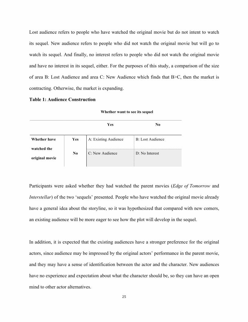
Table 1 outlines the audience relationship between a parent movie and its sequel. Existing

audience refers to people who have watched the original movie and also want to see its sequel.

 

   

25  

Lost audience refers to people who have watched the original movie but do not intent to watch

its sequel. New audience refers to people who did not watch the original movie but will go to

watch its sequel. And finally, no interest refers to people who did not watch the original movie

and have no interest in its sequel, either. For the purposes of this study, a comparison of the size

of area B: Lost Audience and area C: New Audience which finds that B>C, then the market is

contracting. Otherwise, the market is expanding.

Table 1: Audience Construction

Whether want to see its sequel

Yes No

Whether have

watched the

original movie

Yes A: Existing Audience B: Lost Audience

No C: New Audience D: No Interest

Participants were asked whether they had watched the parent movies (Edge of Tomorrow and

Interstellar) of the two ‘sequels’ presented. People who have watched the original movie already

have a general idea about the storyline, so it was hypothesized that compared with new comers,

an existing audience will be more eager to see how the plot will develop in the sequel.

In addition, it is expected that the existing audiences have a stronger preference for the original

actors, since audience may be impressed by the original actors’ performance in the parent movie,

and they may have a sense of identification between the actor and the character. New audiences

have no experience and expectation about what the character should be, so they can have an open

mind to other actor alternatives.

 

   

26  

H3a: People who have watched a parent movie will go to watch its sequel earlier than people

who did not watch the parent movie.

H3b: Compared with new audiences, people who have watched the parent movie have greater

preference to see the original leading actor star in the sequel.

In order to test the generalization of the research findings, the condition for the two movies were

tested separately, replicating the same process.

H4: The attributes’ effect on sequels is constant across different movies.

 

 

   

27  

Chapter 4: Methodology

4.1 Type of study

This study uses the Discrete Choice Experiment (DCE) method to understand individuals’

preference of when to go to theatres to watch sequel movies. Two recently released movies were

chosen for the experiment: Edge of Tomorrow and Interstellar.

There are four reasons to choose these two movies. First, they do not have any actual sequel

movies (nor are they sequel movies themselves), so we can directly test the effect of the parent

movie on its sequel. Otherwise, it would not be clear whether the effect is from the parent movie

or any one of its sequel movies. Secondly, these two movies both only have one leading actor.

Given that one of the objectives was to test whether changing the leading actor would affect an

individual’s watching decision, if there is more than one leading actor, the study would be more

complicated. Thirdly, the two movies were released in 2014. People may have a stronger

impression about a movie that was only recently released. As the survey participants were

university students they would be generally more familiar with recently released movies than

with older ones. Fourthly, both movies have good box office preference. Studios are more likely

to produce a sequel for a movie that earns high box office revenues. Finally, the two movies both

have an open ending so are likely to have sequels. Therefore, it is logical to introduce possible

sequels. Table 2 and Table 3 summarized the basic information of the two parent movies.

The DCE study was designed with seven attributes: title strategy, recommendation, valence,

volume, budget, theatre type and price (Table 4). The attributes are common for both movies

with the exception of title strategy. In addition, with the exception of the actor attribute, which

 

   

28  

has three levels, the attributes only have two levels (Please see Appendix A).

Table 2: Summary (Edge of Tomorrow)

Domestic Total Gross: $100,206,256 Leading Actor: Tom Cruise

Distributor: Warner Bros. Release Date: June 6, 2014

Genre: Sci-Fi Action Runtime: 1 hrs. 53 min.

MPAA Rating: PG-13 Production Budget: $178 million

Plot: Cage (Tom Cruise), a man who is forced onto the front lines for a major military

operation against invading aliens known as “Mimics.” Untrained and unprepared for

combat, Cage is killed within minutes – only to wake up 24 hours earlier with no choice

but to relive (and die) the same day over and over.

Table 3: Summary (Interstellar)

Domestic Total Gross: $188,020,017 Leading Actor: Matthew McConaughey

Distributor: Paramount Release Date: November 5, 2014

Genre: Sci-Fi Adventure Runtime: 2 hrs. 49 min.

MPAA Rating: PG-13 Production Budget: $165 million

Plot: When humanity is facing extinction, an ex-engineer Coop (Matthew McConaughey)

becomes an astronaut who leads the interstellar journey through a wormhole to finding a

new home for the human race.

 

   

29  

Table 4: Attributes and ranges for the “sequel” movies

1. Title Strategy: Named or Numbered title

The movie Interstellar was assigned a sequel with a named title: Interstellar: A New World,

while the movie Edge of Tomorrow was assigned a sequel with a numbered title: Edge of

Tomorrow 2

2. Whether Recommended by Friends: Yes or No

3. Audience Review (valence: 55% or 85%; volume: 20,000 ratings or 100,000 ratings)

This attribute contains two branches. One is valence and the other is volume. Valence has two

levels: 55% and 85%, where 55% represents a medium level rating, and 85% is a high level

rating. Volume also has two levels: 20,000 total user ratings and 100,000 total user ratings,

where 20,000 represent a medium quantity of user ratings, and 100,000 is a large quantity of

user ratings. The ranges were defined based on information retrieved from Rotten Tomatoes:

http://www.rottentomatoes.com/.

4. Production Budget (million) (Interstellar: A New World $110 or $220; Edge of

Tomorrow 2: $120 or $240)

For both sequels, the budget of the parent movie is in the middle of the two levels. $110

million and $120 million represent a low level budget, while $220 million and $240 million

represent a high level budget.

5. Theatre Type (IMAX or Conventional theatres)

6. Ticket Price (IMAX: $14 or $16; conventional theatres: $6 or $8)

Based on the actual ticket price on Tuesday.

7. Leading Actors: (Interstellar: Matthew McConaughey / Joe Manganiello / Ben Affleck;

Edge of Tomorrow: Tom Cruise / Zachary Quinto / Brad Pitt)

This attribute has three levels. In some instances, the leading actor that appeared in the parent

movie was indicated for the ‘sequel’ and in other instances, one of two substitutes; one a well-

known actor and the other lesser-known actor (based on IMDb’s ranking of Most Popular

Males) was used.

 

   

30  

4.2 Sample Size

The   next   step   was   to   decide   how   many   participants   should   be   recruited.   The   study  

calculated  the  sample  size  based  on  the  following  equation.  

DCE sample size calculation:

assuming:

z =1.96, 95% confidence level

p=0.5, 2 option alternatives

q=1-p=0.5, the probability of an unselected option

r=12, the number of choice sets

a=0.05, sample error

n ≥ 32

Therefore, at least 32 participants should be recruited in the study.

4.3 Procedure

Undergraduate students at the University of Guelph were recruited as study participants. They

were told that in the survey was about their choice preference of sequel movies, and that it would

take approximately 15 minutes to complete. In the first part of the survey, respondents were

asked general questions which investigated their movie watching habits, such as when was the

last time they had watched a movie in the theatre, and what is the name of that movie. They were

also asked whether they had watched Interstellar and Edge of Tomorrow. If they had, when and

 

   

31  

where did they see the movies? In the second part of the survey, the two movies (Interstellar and

Edge of Tomorrow) were introduced to them separately. For each movie, background

information about the parent movie was provided, including plot, leading actor, production

budget, MPAA rating and genre. In addition, there was a brief introduction of the plot for the

sequel that was fabricated, in order to offer participants some context for a sequel. After giving

brief information on both the parent movie and its sequel the participants were presented with the

12 DCE choice sets. Under each choice set, the features of the ‘sequel’ were described in several

short points following which respondents were asked when they would go to the theatre to watch

this sequel (See Appendix B). Participants completed the DCE for Edge of Tomorrow, and then

repeated the procedure for Interstellar. After completion of all of the DCE questions, there was

one demographic question asking them to indicate their gender.

4.4 Model

Uij = Vij + εij

In the Random Utility Model, Uij is the utility that an individual i receives from an alternative j.

Vij is the deterministic component, which is the utility an alternative j can provide to an

individual i. εij is the random and unobservable error associated with individual i’s choice of

alternative j.

The deterministic part of the model Vij is manipulated in the following equations:

Vi = β0Interstellar + β1Recommendi + β2Valencei +β3Volumei + β4Budgeti + β5Theatrei + β6 Pricei

+β7Matthew + β8Ben + β9Tom + β10 Brad

where:

• Vi is the preference for when to watch a sequel in the theatre

 

   

32  

• Interstellar is 1 when the movie is Interstellar and -1 when movie is Edge of

Tomorrow

• Recommendi is 1 when the movie is recommended by friends and -1 when the movie is

not recommended by friends

• Valencei is 1 when the audience review is 85% and -1 when the audience review is

55%

• Volumei is 1 when the total postings are 100,000 and -1 when the total postings are

20,000

• Budgeti is 1 when the production budget is high ($220 million or $240 million) and -1

when the production budget is low ($110 million or $120 million)

• Theatrei is 1 when the theatre type is IMAX and -1 when the theatre type is

conventional theatres

• Pricei is high: $16 / $8 or low: $14 / $6

• Matthew is 1 when the leading actor is Matthew McConaughey, 0 when the leading

actor is Ben Affleck and -1 when the leading actor is Joe Manganiello

• Ben is 1 when the leading actor is Ben Affleck, 0 when the leading actor is Matthew

McConaughey and -1 when the leading actor is Joe Manganiello

• Tom is 1 when the leading actor is Tom Cruise, 0 when the leading actor is Brad Pitt

and -1 when the leading actor is Zachary Quinto

• Brad is 1 when the leading actor is Brad Pitt, 0 when the leading actor is Tom Cruise

and -1 when the leading actor is Zachary Quinto

 

   

33  

This equation calculates the probability that an individual would choose one alternative over

another. In this study there were two alternatives: to watch the sequel movies in the theatre or

not. The variable yi refers to an individual i’s movie attendance decision. It was assumed that yi

is 1 if an individual planed to watch the sequel in the theatre and 0 if the individual will not go to

theatre to see the sequel.

 

   

34  

Chapter 5: Research Findings

The study recruited 154 students from the University of Guelph as participants. All data

collected was usable. As part of the survey, participants were asked “what type of movie do you

most likely to watch in the theatre” The results demonstrate that action (77%), comedy (75%)

and adventure (58%) are the three most popular genres among all the types presented to this

group of participants. Only one social-demographic question was included at the end of the

survey: Gender, and 75% of the participants were male, while 25% were female. Given that the

study tested participants’ reaction to the level changes, a high proportion of male did not affect

the results of the experiment.

5.1 Edge of Tomorrow

5.1.1 H1 and H2 (Null Partially rejected)

The effect of each attribute on participants’ decision of whether to watch the sequel in the

theatres was examined first (Table 5). The results indicate that only four of the attributes:

Recommend (p=0.013), Valence (p=0.000), Actor 2 (p=0.051) and Parent (p=0.000) had a

significant effect on participants’ decision. According to the Prob equation, it was determined

that people are 5.80% more likely to watch Edge of Tomorrow 2 if this movie is recommended

by their friends than if not recommended. People are 10.76% more likely to watch Edge of

Tomorrow 2 when its parent movie “Edge of Tomorrow” got positive audience score, compared

with the parent movie that got negative audience score. People are 7.24% more likely to watch

Edge of Tomorrow 2 if the movie uses Brad Pitt as its leading actor as opposed to using Zachary

Quinto. People who have watched Edge of Tomorrow are 13.46% more likely to watch Edge of

Tomorrow 2 than those who did not watch the parent movie. Figure 1 demonstrates the level

comparisons of the significant attributes.

 

   

35  

Table 5: Attributes affect on whether to watch Edge of Tomorrow 2

Parameter B SE Wald Sig. Exp(B) Recommend 0.114 0.046 6.18 0.013 1.121 Valence 0.216 0.038 32.179 0.000 1.241 Volume 0.041 0.11 0.136 0.712 1.042 Budget -0.045 0.114 0.156 0.693 0.956 Theatre 0.725 1.203 0.363 0.547 2.065 Price -0.019 0.055 0.123 0.726 0.981 Actor1(1) 0.065 0.072 0.805 0.370 1.067 Actor2(2) 0.145 0.074 3.802 0.051 1.156 Parent(3) 0.271 0.074 13.574 0.000 1.311 Price*theatre -0.069 0.091 0.57 0.450 0.933 (1) Actor1=Tom Cruise (2) Actor2=Brad Pitt (3) Parent=whether watched the parent movie

Figure 1: Comparisons of levels for the significant attributes I (Edge of Tomorrow 2)

 

 The attributes that influence individuals’ decision of when to watch Edge of Tomorrow 2 (Table

6) were investigated. In the analysis of whether they would watch the sequel, participants’ choice

fit into one of two categories: watch or not watch. But in the analysis of when they would watch

the sequel, participants’ date selection was taken into consideration. Results show that five

attributes have a significant impact: Actor1 (p=0.0011), Actor2 (p<0.0001), Recommend

(p<0.0001), Valence (p<0.0001) and Parent (p=0.0017). Figure 2 depicts how the significant

attributes affect an individual’s movie watching intention. If the sequel is recommended by

0.2

0.3

0.4

0.5

0.6

yes no 85% 55% Pitt Quinto yes no

Recommend Valence Actor2 Parent

 

   

36  

friends, participants were 7% more likely to watch this movie. If the parent movie got a positive

audience score, participants were 18.35% more likely to watch the sequel. Participatns were

7.14% more likely to watch Edge of Tomorrow 2, when the sequel still uses Tom Cruise as its

leading actor, instead of Zachary Quinto. Meanwhile, if the sequel uses Brad Pitt as its leading

actor, participants were 9.43% more likely to watch the movie. If the participants had watched

the parent movie, they were 32.82% more likely than new comers to indicate that they would

watch the sequel.

 Table 6: Attributes affect on when to watch Edge of Tomorrow 2

Parameter Estimate SE t Value Pr > |t| Intercept 2.600 0.34 7.56 <.0001 Recommend -0.140 0.03 -5.55 <.0001 Valence -0.371 0.03 -13.37 <.0001 Volume -0.005 0.05 -0.10 0.9226 Budget -0.026 0.03 -0.80 0.4271 Theatre 0.101 0.12 0.81 0.4206 Price 0.015 0.03 0.52 0.6046 Actor1(1) -0.143 0.04 -3.31 0.0011 Actor2(2) -0.189 0.04 -4.39 <.0001 Parent(3) -0.682 0.21 -3.19 0.0017 (1)Actor1=Tom Cruise (2)Actor 2=Brad Pitt (3)Parent=whether watched the parent movie

The results of whether and when to watch the sequel were compared and it was found that the

attributes which affect whether to watch the sequel also influence when to watch the sequel.

Also, one more attribute is significant in the analysis of when to watch: Actor1. As a result,

H1(b)/H2(b) and H1(e)/H2(e) were rejected, which means that recommend and actor both have

positive and significant effects on the sequel’s audience size and life cycle. Since only valence

and not volume was found to have a significant effect, H1(c)/H2(c) were partially rejected.

Valence had a positive and significant effect on participants’ preference. Budget, theatre and

 

   

37  

price were not found to have significant impacts, so H1(d)/H2(d), H1(f)/H2(f) and H1(g)/H2(g)

were not rejected.

Figure 2: Comparisons of the levels for significant attributes II (Edge of Tomorrow 2)

Based on the estimates in Table 6, the following utility equation was derived.

U=2.6 - 0.140Recommend – 0.371Valence – 0.005Volume – 0.026Budget + 0.101theatre + 0.015Price –

0.143Tom – 0.189Brad +ε

Table 7: Attributes affect on intention to watch Edge of Tomorrow 2 (existing audience

only)

Paraeter B SE Wald Sig. Exp(B) Recommend 0.102 0.084 1.466 0.226 1.108 Valence 0.162 0.071 5.156 0.023 1.176 Volume 0.012 0.207 0.003 0.954 1.012 Budget -0.001 0.217 0 0.995 0.999 Theatre 0.329 2.287 0.021 0.886 1.389 Price -0.019 0.103 0.035 0.852 0.981 Price*theatre -0.026 0.175 0.023 0.88 0.974 Actor1(1) 0.134 0.134 1.002 0.317 1.144 Actor2(2) 0.017 0.141 0.015 0.904 1.017

(1)Actor1=Tom Cruise (2)Actor 2=Brad Pitt

0.535

0.465

0.592

0.408

0.536

0.464

0.547

0.453

0.664

0.336

0.2

0.3

0.4

0.5

0.6

0.7

yes no 85% 55% CruiseQuinto Pitt Quinto yes no

Recommend Valence Actor1 Actor2 Parent

 

   

38  

Since whether the parent movie has been watched had a very significant effect on participants’

choice of whether and when to watch its sequel, focus was put onto participants who had

watched the parent movie, to investigate factors that affected their movie watching decision

(Table 7). The results indicate that the only significant attribute is Valence (p=0.023), which

means for participants who had watched Edge of Tomorrow, the only attribute which affected

their decision of whether to watch Edge of Tomorrow 2 was audience score of the parent movie.

The results indicate that existing audience was only influenced by valence, while new audience

was affected by more attributes: recommendation, actor and valence. This may be because

existing audience, who have watched the parent movie already have their own evaluation about

the movie, so their decision of whether to watch the sequel depends on whether they are attracted

by the storyline. The only thing they want to do is to compare their own evaluation with the

audience score given by many other audience to see if they reach the same evaluations of the

parent movie with those of the general public. However, for new audience, who know little about

the story of the parent movie, are more likely to rely on more movie features to decide whether it

is worth watching the sequel.

5.1.2 Audience size

According to the estimates in Table 6, the combination levels of the best features and worst

features were determined (Table 8). For example, the attribute “recommendation” positively

effect participants’ choices, so the level coded as “1” went to the best-feature combination.

While the level coded as “-1” went to the worst-feature combination. In Table 8, the column

headed “Best features’ shows the highest probability of watching Edge of Tomorrow 2

(P=0.922). Based on the setting of attributes and their levels, 92.2% of individuals were likely to

 

   

39  

watch a sequel if they had watched the parent movie, and if this sequel was recommended by

other people, had received a total of 100,000 audience ratings and its parent movie had an

audience score of 85%, had a $240 million production budget, shows in conventional theatres

with $6 ticket price, and uses Brad Pitt as its leading actor. The column headed ‘Worst features’

shows the lowest probability of attendance at theatres to watch this sequel (P=0.111), which

means that 11.1% of participants were likely to watch Edge of Tomorrow 2, if they had not seen

the parent movie and this sequel was not recommended by friends, received only 20,000

audience ratings and its parent movie had an audience score of 55%, had a $120 million

production budget, shows in IMAX theatres with a $16 ticket price, and uses Zachary Quinto

(who is not considered famous) as its leading actor. The last column headed ‘Parent movie’

presents the probability of watching the parent movie (P=0.849), according to the actual movie

data. With the probability of watching the parent movie falling between the two extremes of

watching its sequel, this suggests that whether this sequel can expand the audience size depends

on the combinations of levels of the attributes.

 Table 8: The Probability of Watching Edge of Tomorrow 2

Attributes Best features Worst features Parent movie Actor1 0 -1 1 Actor2 1 -1 0 Recommend 1 -1 -1 Valence 1 -1 1 Volume 1 -1 1 Budget 1 -1 -0.03 Theatre -1 1 -1 Price 6 16 8 Parent 1 -1 1 Probability 0.922 0.111 0.849

 

   

40  

Table 9 shows the probability distribution of movie watching for both the best-feature and worst-

feature combinations. The results indicate that the best-feature combination attracts more

attendance from category 1 to 6. On the other hand, in the worst-feature combination, more

participants show little interest in watching Edge of Tomorrow 2 in the theatres. Almost 90% of

participants chose to wait for the DVD release to never watch this sequel.

Table 9: The probability distribution (Edge of Tomorrow 2)

Category 1(1) 2(2) 3(3) 4(4) 5(5) 6(6) 7(7) 8(8)

Prob (best features) 0.120 0.202 0.229 0.220 0.095 0.057 0.075 0.003 Prob (worst features) 0.000 0.001 0.005 0.023 0.033 0.049 0.452 0.437 (1) 1=First day (2) 2=Second day (3) 3=Third day to seventh day (4) 4=Second week (5) 5=Third week (6) 6=Fourth week (7) 7=I will wait for DVD release or other sources (8) 8=I will never see this sequel

5.1.3 Product life Cycle

The average attendance rate (for the Edge of tomorrow sequel) across all 12 level combinations

was calculated and Figure 3 shows the attendance rate in the first month. The audience

attendance was predicted to be 19.6% during the first week, 12.6% during the second week,

8.7% during the third week and 8% during the fourth week. As a result, the attendance decrease

rate is 35.8% from the first week to the second week, 30.5% from the second week to the third

week, and 8.6% from the third week to the fourth week (Table 10). The actual weekly decrease

rates of its parent movie were 41.5%, 37.7% and 43.9%, respectively

(http://www.boxofficemojo.com/). Comparison of these decreasing rates indicates that the parent

movie and its sequel have a similar life cycle pattern, and the sequel does not have a shorter

lifetime.

 

   

41  

Figure 3: Average Attendance rate predicted for Edge of Tomorrow 2

Table 10: Weekly Attendance Change Rate (Edge of Tomorrow)

Week 1 to Week 2 Week 2 to Week 3 Week 3 to Week 4 Average -35.8% -30.5% -8.6% Parent -41.5% -37.7% -43.9% Best-feature Combination -60.1% -50.8% -40.0%

Figure 4: Weekly Attendance Change Rate (Edge of Tomorrow)

The life cycle of the sequel that adopts the best-feature combination was then investigated. Based

on the results in Table 7, weekly attendance in the first month was predicted (figure 5). The

figure shows that the attendance rate is 55.1% in the first week, 22% in the second week, 9.6% in

the third week and 5.7% in the fourth week. The attendance decrease rates are 60.1% from the

first week to the second week, 50.8% from the second week to the third week, and 40% from the

0%

5%

10%

15%

20%

25%

1 2 3 4 Week

0"

0.1"

0.2"

0.3"

0.4"

0.5"

0.6"

1" 2" 3" 4"

Average"

Parent"

Best5feature"

 

   

42  

third week to the fourth week (Table 10). Compared with the expected weekly decrease rate for

Edge of Tomorrow, this sequel dies quicker than its parent movie, suggesting that the sequel has

a shorter life cycle.

Figure 5: Attendance rate of the best-feature combination (Edge of Tomorrow 2)

The analysis of the responses on intention to see the sequel indicate that the life cycle of the

sequel depends on the level combinations (Table 10 and Figure 4). If the sequel has the best level

combination, the audience may go to see the sequel earlier. As a result, the movie will have a

faster attendance decrease rate from week to week, and a shorter lifecycle is anticipated.

5.1.4 Hypothesis 3a (Supported)

H3a: People who have watched a parent movie will go to watch its sequel earlier than people

who did not watch the parent movie.

H3 investigates the effect of having seen the parent movie. Participants were divided into two

groups: existing audience (people who have watched the parent movie) and new comers (people

who did not watch the parent movie). H3 was tested by comparing when the participants from

each group indicate that they would go to theatre to see the sequel. It is anticipated that audiences

0%

10%

20%

30%

40%

50%

60%

1 2 3 4 Week

 

   

43  

who had seen the parent movie are more eager to watch sequels and would go earlier than new

comers who hadn’t seen the parent movie. Figure 6 depicts the average attendance comparisons

in the first day, first week and later weeks (Complete comparison data is available in Appendix

C). In the figure, “YES” refers to the “existing audience” group, while “NO” refers to the “new

comers” group. The vertical axis represents the proportion of moviegoers.

Figure 6: Attendance Comparisons (Edge of Tomorrow 2)

The average anticipated attendance by the existing audience in the first week is 47.9%,

accounting for almost half of the total theatre attendance, while the attendance for the newcomer

group is only 36.9%. The attendance difference is much larger in the first day comparison. The

average first day attendance for the existing audience is 19.7%, while for the newcomer group is

only 6.6%. From this, there would be a higher percentage of new comers who chose to see the

sequel after the first week. The attendance of the two groups in the rest weeks of the first month

was compared. Figure 6 illustrates that new comers are more likely to watch the sequel in the

second, third and fourth weeks than is the existing audience. It is quite clear that the existing

audience are tend to watch sequels earlier than new comers, so the H3a is supported.

 

   

44  

5.1.5 H3b (Not supported)

H3b: Compared with new audiences, existing audiences have greater preference to see the

leading actor in the parent movie star in the sequel.

The hypothesis was tested by investigating the interaction effect of parent and actors. Table 11

presents the estimated results. It was found that the interaction effect of Actor1*Parent and

Actor2*Parent are both not significant, suggesting that for the existing audience, they do not

have a strong preference for the original leading actor. So H3b is not supported.

Table 11: Interaction effect (Edge of Tomorrow)

Parameters B SE Wald Sig. Exp(B) Recommend 0.114 0.046 6.178 0.013 1.121 Valance 0.216 0.038 32.179 0 1.241 Volume 0.041 0.11 0.136 0.713 1.042 Budget -0.045 0.114 0.156 0.693 0.956 Theatre 0.725 1.203 0.362 0.547 2.064 Parent(1) 0.273 0.074 13.617 0 1.314 Actor1(2) 0.04 0.078 0.259 0.611 1.041 Actor2(3) 0.181 0.08 5.173 0.023 1.198 Price -0.019 0.055 0.123 0.726 0.981 Price*Theatre -0.069 0.091 0.569 0.451 0.933 Actor1*Parent 0.087 0.102 0.736 0.391 1.091 Actor2*Parent -0.129 0.104 1.547 0.214 0.879

(1) Parent=whether watched the parent movie (2) Actor1=Tom Cruise (3) Actor2=Brad Pitt

 

   

45  

5.2 Interstellar: A New World

5.2.1 H1 and H2 (Null Partially rejected)

As with the sequel, Edge of Tomorrow 2, there are also four variables which were found to have

a significant impact on participants’ movie watching decisions (Table 12): Recommend

(p=0.019), Valence (p=0.000), Actor 1 (p=0.022) and Parent (p=0.001). Participants were 5.2%

more likely to watch Interstellar: A New World if they were told that their friends recommend

this movie. Participants were 6.4% more likely to watch this sequel when its parent movie,

Interstellar had a positive audience score than when the parent movie had a negative audience

score. Participants were 7.8% more likely to watch Interstellar: A New World if the movie were

to have the original actor from the parent movie, Matthew McConaughey, as its leading actor

rather than if the lesser-known Joe Manganiello was the lead actor. Participants who had

watched Interstellar were 10.6% more likely to watch Interstellar: A New World than those who

had not watch the parent movie. Figure 7 presents the comparison of the levels of the four

attributes.

Table 12: The effect of each attribute (Interstellar: A New World)

B SE Wald df Sig. Exp(B) Recommend 0.103 0.044 5.461 1 0.019 1.108 Valence 0.13 0.036 13.248 1 0.000 1.139 Volume 0.004 0.104 0.002 1 0.966 1.004 Budget 0.046 0.11 0.175 1 0.675 1.047 Theatre -0.042 1.173 0.001 1 0.971 0.959 Price -0.019 0.052 0.139 1 0.709 0.981 Actor1(1) 0.154 0.067 5.235 1 0.022 1.167 Actor2 (2) 0.028 0.069 0.169 1 0.681 1.029 Parent(3) 0.214 0.063 11.558 1 0.001 1.238 Price*theatre 0.001 0.089 0 1 0.994 1.001

(1) Actor1=Matthew McConaughey (2) Actor2=Ben Affleck (3) Parent=whether watched parent movie

The attributes that influence a participant’s preference of when they would watch Interstellar: A

 

   

46  

New World was investigated (Table 13). Attributes identified as having a significant impact on

participants’ movie watching decision were the same as those for Edge of Tomorrow 2:

Recommend (p<0.0001), Valence (p<0.0001), Actor1 (p<0.0001) and Parent (p=0.0022). If the

sequel was reported as recommended by friends, Participants were 9.2% more likely to watch it.

If the parent movie had a positive audience score, participants were 14.73% more likely to watch

the sequel. Participants were 20.66% more likely to watch Interstellar: A New World, when this

sequel used Matthew McConaughey as its leading actor instead of the less famous actor, Joe

Manganiello. If the participants had watched the parent movie, they were 32.82% more likely

then new comers to watch the sequel. Figure 8 shows the comparison of the levels of the four

attributes.

Figure 7: Comparisons of the levels of significant attributes I (Interstellar: A New World)

With the results noted above, H1(b)/H2(b) and H1(e)/H2(e) are both rejected, since both

recommend and actor had a positive and significant effect on the sequel’s audience size and life

cycle. The audience review attribute has both valence and volume. Since valence was the only

variable found to have a significant effect, so H1(c)/H2(c) was partially rejected. Since no

significant effects were found for budget, theatre and price, H1(d)/H2(d), H1(f)/H2(f) and

H1(g)/H2(g) were not rejected.

0.5260.474

0.532

0.468

0.538

0.461

0.553

0.447

0.2

0.3

0.4

0.5

0.6

yes no 85% 55% Matthew Joe yes no

Recommend Valence Actor1 Parent

 

   

47  

Based on the estimates in Table 11, the following utility equation was derived:

U=2.018 - 0.185Recommend – 0.297Valence – 0.068Volume – 0.008Budget - 0.006theatre + 0.047Price

– 0.419Matthew – 0.048Ben +ε

Table 13: Attributes that affected when to watch Interstellar: A New World

Parameter Estimate SE t Value Pr > |t| Intercept 2.018 0.34 5.90 <.0001 Recommend -0.185 0.03 -7.34 <.0001 Valence -0.297 0.03 -10.91 <.0001 Volume -0.068 0.05 -1.39 0.167 Budget -0.008 0.03 -0.26 0.7961 Theatre -0.006 0.12 -0.05 0.9593 Price 0.047 0.03 1.63 0.1046 Actor1(2) -0.419 0.04 -9.69 <.0001 Actor2(3) -0.048 0.04 -1.13 0.2601 Parent(1) -0.556 0.18 -3.11 0.0022

(1) Actor1= Matthew McConaughey (2) Actor2=Ben Affleck (3) Parent=whether watched the parent movie

Figure 8: Comparisons of levels of the significant attributes II (Interstellar: A New World)

In addition, the factors that affect individuals who have watched the parent movie were

investigated. It was found that only Valence (p=0.025) is a significant attribute (Table 14), which

means that for participants who had watched Interstellar, audience score of the parent movie was

the only variable which affected their choice of whether to watch Interstellar: A New World or

not. Participants were 5.98% more likely to watch Interstellar: A New World, when its parent

0.2

0.3

0.4

0.5

0.6

yes no 85% 55% Matthew Joe yes no

Recommend Valence Actor1 Parent

 

   

48  

movie had received a positive audience score.

Table 14: The effect of each attributes (existing audience only)

B SE Wald Sig. Exp(B)

Recommend 0.075 0.064 1.377 0.241 1.078 Valence 0.119 0.053 5.017 0.025 1.127 Volume 0.019 0.153 0.015 0.902 1.019 Budget 0.026 0.161 0.026 0.873 1.026 Theatre 0.013 1.712 0 0.994 1.013 Price -0.026 0.076 0.112 0.738 0.975 Theatre*price -0.001 0.131 0 0.991 0.999 Actor1(1) 0.109 0.1 1.199 0.274 1.115 Actor2(2) 0.022 0.102 0.045 0.833 1.022

(1) Actor1= Matthew McConaughey (2) Actor2= Ben Affleck

 

5.2.2 Audience Size

According to the estimated results in Table 12, the probability of watching the parent and the

sequel movies was calculated (Table 15). The “Best feature” column shows the highest

probability of watching Interstellar: A New World (P=0.917). This probability indicates that

participants were 91.7% likely to go to watch Interstellar: A New World, if all of the following

are taken as true: they had watched the parent movie, the sequel is recommended by other people

and recieved a total of 100,000 audience ratings, its parent movie had received an audience score

of 85%, the sequel had a $220 million production budget, is shown in IMAX theatres with a $14

ticket price, and still uses Matthew McConaughey as its leading actor. The “Worst feature”

column shows the lowest probability of going to theatres to watch this sequel is (P=0.183),

which means that participants were 18.3% likely to watch Interstellar: A New World, if all of the

following were taken as true: they had not watched the parent movie, this sequel was not

recommended by friends, the sequel had 20,000 audience ratings and its parent movie had

received an audience score of 55%, the sequel had a $110 million production budget, shows in

 

   

49  

conventional theatres with an $8 ticket price, and the sequel used a lesser-known actor, Joe

Manganiello, as its leading actor. The “Parent movie” column presents the probability of

watching the parent movie, according to its actual movie data is (P=0.899). The results indicated

that, similar with Edge of Tomorrow 2, whether this sequel can expand the audience size also

depends on the combination of the levels of the attributes.

Table 15: The Probability of Watching Interstellar: A New World

Attributes Best features Worst features Parent movie Actor1 0 -1 1 Actor2 1 -1 0 Recommend 1 -1 -1 Valence 1 -1 1 Volume 1 -1 1 Budget 1 -1 0 Theatre 1 -1 -1 Price 14 8 8 Parent 1 -1 1 Probability 0.917 0.183 0.899

Table 16: The probability distribution (Interstellar: A New World)

Category 1(1) 2(2) 3(3) 4(4) 5(5) 6(6) 7(7) 8(8)

Prob (best features) 0.127 0.160 0.250 0.193 0.109 0.078 0.081 0.002 Prob (worst features) 0.000 0.002 0.012 0.033 0.050 0.085 0.535 0.282 (1) 1=First day (2) 2=Second day (3) 3=Third day to seventh day (4) 4=Second week (5) 5=Third week (6) 6=Fourth week (7) 7=I will wait for DVD release or other sources (8) 8=I will never see this sequel

Table 16 shows the probability distribution of movie watching for both the best-feature and

worst-feature level combinations. Categories 1 to 8 refer to the eight choices for watching the

sequel in the survey. The results indicate that the best-feature combination attracts more

attendance in the first 3 weeks of the movie playing. While in the worst feature group, more

 

   

50  

participants choose not to watch the sequel in the theatres.

5.2.3 Product life cycle

Figure 9 shows the average expected attendance rate of this sequel in the first month. Analysis

demonstrates that the attendance rate is predicted to be 24.5% during the first week, 11.4%

during the second week, 9.31% during the third week and 9.96% during the fourth week. As a

result, the attendance decrease rate is 53.4% from the first week to the second week and 18.5%

from the second week to the third week. However, from the third week to the fourth week, the

attendance rate increases by 7% (Table 17). The weekly decrease rates of its parent movie are

44.4%, 30.5% and 24.7%, respectively (http://www.boxofficemojo.com/). Comparison shows

that, in general, the parent movie has a faster decrease rate than that expected for the sequel.

Figure 9: Average Attendance rate of Interstellar: A New World

Table 17: Weekly Attendance Change Rate (Interstellar: A New World)

Week 1 to Week 2 Week 2 to Week 3 Week 3 to Week 4 Average -54.30% -18.50% +7% Parent -44.40% -30.50% -24.70% Best-feature Combination -64.10% -43.50% -28.40%

0%5%

10%15%20%25%30%35%

1 2 3 4 Week

 

   

51  

Figure 10: Weekly Attendance Change Rate (Interstellar: A New World)

The life cycle of the sequel that adopts the best-feature combination was also investigated

(Figure 11). Analysis shows that the attendance rate is 53.7% in the first week, 19.3% in the

second week, 10.9% in the third week and 7.8% in the fourth week. The attendance decrease

rates were 64.1% from the first week to the second week, 43.5% from the second week to the

third week, and 28.4% from the third week to the fourth week (Table 15). The decrease rates

from week to week are all higher than those of its parent movie. It is anticipated that this sequel

may die quicker and have a shorter lifecycle than its parent movie.

Figure 11: Attendance rate of the best-feature combination (Interstellar: A New World)

Similar with the movie Edge of Tomorrow 2, the life cycle of Interstellar: A New World also

depends on the combinations of the levels of the attributes.

0"

0.1"

0.2"

0.3"

0.4"

0.5"

0.6"

1" 2" 3" 4"

Average"

Parent"

Best5feature"

0%

10%

20%

30%

40%

50%

60%

1 2 3 4 Week

 

   

52  

5.2.4 Hypothesis 3a (Supported)

H3a: People who have watched a parent movie will go to watch its sequel earlier than people

who did not watch the parent movie.

To test this hypothesis, the first day, first week and later weeks’ attendances were compared

(Figure 12). The average attendance of existing audience is expected to be 15.9% in the first day,

and 51.7% in the first week compared with the average expected attendance of new comers of

only 9.4% in the first day and 38.3% in the first week. The existing audience had a higher

expected attendance rate in both the first day and the first week. Figure 8 shows the attendance

comparison of later weeks in the first month. The findings confirm that new audiences tend to

watch the sequel later than existing audience, since the attendance of new comers in the later

weeks are higher than for the existing audience. Therefore, according to the three comparisons,

the H3a is supported.

Figure 12: Weekly Attendance Comparison (Interstellar: A New World)

5.2.5 H3b (Not supported)

H3b: Compared with new audiences, existing audiences have greater preference to see the

leading actor in the parent movie star in the sequel.

 

   

53  

For Interstellar: A New World, we test the H3b also by estimate the interaction effect of whether

watched the parent movie and the actors. We also found that the two interaction effects are both

not significant, so the H3b is not supported.

Table 18: Interaction effect (Interstellar: A New World)

Parameters B SE Wald Sig. Exp(B) Recommend 0.103 0.044 5.461 0.019 1.108 Valance 0.13 0.036 13.248 0 1.139 Volume 0.004 0.104 0.002 0.966 1.004 Budget 0.046 0.11 0.175 0.675 1.047 Theatre -0.042 1.173 0.001 0.971 0.959 Actor1(1) 0.198 0.078 6.453 0.011 1.218 Actor2(2) 0.041 0.08 0.258 0.611 1.042 Price -0.019 0.052 0.139 0.709 0.981 Parent(3) 0.225 0.063 12.608 0 1.253 Price*Theatre 0.001 0.089 0 0.994 1.001 Actor1*Parent -0.095 0.086 1.208 0.272 0.909 Actor2*Parent -0.025 0.089 0.078 0.78 0.975

(1) Actor1= Matthew McConaughey (2) Actor2=Ben Affleck (3) Parent=whether watched the parent movie

5.3 H1(a) and H2(a) (Null Rejected)

In this section of the study, Interstellar: A New World is a named title, while in thwe previous

section Edge of Tomorrow 2 is a numbered title. According to Sood and Drèze’ research (2006),

consumers have more favorable attitudes towards a movie that uses a named title than a

numbered title. As a result, participants should show more interest in watching Interstellar: A

New World as compared to Edge of Tomorrow 2. The effect of title strategy was tested from two

dimensions. The first month movie attendance (and the first week and first day attendances were

compared for these two ‘sequels’.

First a comparison was made of the performance of two parent movies from both box office

revenues and online reviews. The two parent movies: Interstellar and Edge of Tomorrow were

 

   

54  

both released in 2014. Interstellar brought in $188,020,017 in box office revenue in the domestic

market, while Edge of Tomorrow brought in $100,206,256 (www.boxofficemojo.com). From the

online review aspect, Interstellar had a 72% critics’ score and 85% audience score, while Edge

of Tomorrow received 90% for both the critics’ score and the audience score. The actual movie

data shows that although Interstellar had higher box office revenue, Edge of Tomorrow is more

favored by audiences and critics. Therefore, the two parent movies have similar spillover effects.

 Table 19: Attendance comparison

Interstellar: A New World Edge of Tomorrow 2

Existing Audience First month 0.624 0.6 First week 0.323 0.287 First day 0.099 0.118 New comers First month 0.504 0.457 First week 0.193 0.169 First day 0.047 0.03 Total First month 0.552 0.491 First week 0.245 0.197 First day 0.068 0.051

Table 19 presents the results of a comparison of attendance rate in three categories: existing

audience, new comers and the entire sample. Since whether having watched the parent movie has

a significant effect on participants’ decision of whether and when to watch its sequel, so in this

part of the analysis, the participants are separated into existing audience and new comers, in

order to see if there is a difference in the attendance rates. The results demonstrate that only in

the first day for the existing audience was the expected attendance rate for Edge of Tomorrow 2

slightly higher than that of Interstellar: A New World. In all other comparisons, the expected

attendance rate of Interstellar: A New World was higher than the rates for Edge of Tomorrow 2,

suggesting that no matter whether it is an existing audience or new comers, participants were

more interested in watching the sequel to Interstellar, and tended to watch this sequel earlier than

 

   

55  

the sequel to Edge of Tomorrow. The effect of the title strategy is confirmed, and we reject the

null hypotheses H1(a) and H2(a).

5.4 Hypothesis 4 (Supported)

H4: The attributes’ effect on sequels is constant across different movies.

Table 20: Comparison of Edge of Tomorrow 2 and Interstellar: A New World

Edge of Tomorrow 2 Interstellar: A New World

Attributes affecting whether to watch the sequel

Recommend Valence Actor2 Parent

Recommend Valence Actor1 Parent

Attributes affecting whether to watch the sequel (Existing audience only)

Valence Valence

Attributes affecting when to watch sequel

Recommend Valence Actor 1 Actor 2 Parent

Recommend Valence Actor1 Parent

Audience Size Sequel VS Parent The highest Psequel > Pparent > The lowest Psequel

The highest Psequel > Pparent > The lowest Psequel

Life Cycle DR(1)

highest-level combination> DRparent > Average DRsequel

DRhighest-level combination> DRparent > Average DRsequel

Existing Audience VS New Comers Movie Attendance Existing audience > New

comers Existing audience > New comers

First Day Attendance

Existing audience > New comers

Existing audience > New comers

First Week Attendance

Existing audience > New comers

Existing audience > New comers

Later Weeks Attendance

New comers > Existing audience

New comers > Existing audience

(1) DR=decrease rate

H4 aims to confirm the generality of the research findings. We test this hypothesis by testing

whether the results for the two movies have similar patterns. Table 20 presents the comparison of

the results. Except for the items “attributes affecting whether to watch the sequel” and “attributes

affecting when to watch sequel”, the two movies had the same pattern of results. For the decision

 

   

56  

of whether and when to watch the sequel, the only difference is in the attribute: actor. In Edge of

Tomorrow 2, using a famous actor (Actor 2) to replace the original leading actor also has a

positive and significant effect. But in Interstellar: A New World, only the original leading actor

has a significant impact on attracting the audience to watch the sequel. Although there is a

difference in which actor can influence audiences’ movie watching decision, in general, they

both highlight that the attribute “actor” can affect an individual’s preference of whether and

when to watch the sequel. Therefore, from the comparison table, we conclude that the H4 is

supported.

 

 

   

57  

Chapter 6: Discussions and Conclusions

The four objectives in this study were: First, detecting attributes that significantly influence a

sequel’s audience size and life cycle. Secondly, determining whether people who have watched

the parent movie are eager to watch its sequel earlier. Third, investigating whether a sequel that

uses a named title attracts more audience than a sequel, which uses a numbered title. Lastly,

testing the generalization of the results. The major findings of this study are summarized in this

chapter.

6.1 Attributes effects

Examination of the attributes that affect an individual’ decision of whether to watch the sequel in

the theatre revealed that the attributes: recommend, valence, actor and title strategy have

significant effects. The attributes that affect an individual’s preference of when to watch the

sequel in the theatres were found to be the same significant attributes of recommend, valence and

actor. Examination of the attributes that affect audiences who have watched the parent movie

showed that only the valence attribute is significant. Previous research shows that

recommendation (Wang, 2005), volume (Liu, 2006), valence (Basuroy et al, 2003), budget

(Elberse, 2013) and actor (Ravid, 1999) all have significant effects on a movie’s financial

success. However, in the current study, neither volume nor budget is significant for participants’

date choice.

6.1.1 Recommendation

In both Edge of Tomorrow 2 and Interstellar: A New World, recommendation is a significant

attribute that influences an individual’s decision of whether and when to watch a sequel,

indicating that an individual’s choice is largely influenced by people around him/her.

 

   

58  

6.1.2 Valence

In the current study, the audience score of the parent movie is the only attribute that is significant

in all three analyses. Whether the audience rating of the parent movie is positive or negative

significantly affects an individual’s movie watching decision. Specifically, for an existing

audience, valence is the only significant attribute, suggesting that only the valence can be a

reference to help an existing audience decide whether to watch the sequel in the theatres,

whereas a change of any other movie attributes has little impacts on the decision.

6.1.3 Actor

This is the only attribute in this study, which has three levels. As well as the original leading

actor, this study used a famous actor and a lesser-known actor as two alternatives for the leading

role in the sequel. For Edge of Tomorrow 2, the original actor and the famous alternate actor both

show significant effects on intention to see the sequel, while for Interstellar: A New World, only

the original actor is significant. The lesser-known actor alternative is not significant in either

movie. The results indicate that for a sequel, audience prefers its original leading actor or other

notable movie stars.

6.1.4 Volume

Volume is not a significant attribute in the analysis, although some recent papers emphasize the

explanatory power of volume, rather than valence, on box office revenue (Chen et al 2004; Liu,

2006). The results from the current study, however, indicate that both existing audience and new

comers place a higher value on how audiences have evaluated the parent movie, rather than the

size of the audience of the parent movie.

6.1.5 Budget

As with volume, budget is another insignificant attribute. Although earlier literature on movie

 

   

59  

attendance has found a positive relationship between production budget and box office revenue,

audiences may have no knowledge of how the budget can make a difference, or in other words,

the general public cannot tell the difference between a $100 million and a $200 million

production budget movie. Budget supports a movie at all aspects, but the audience seems more

likely to rely on external features (i.e. leading actor) to judge a movie.

6.1.6 Theatre

Theatre is a new attribute that has not been used in previous studies, but was added to the current

one to see if intention to see a movie is affected by whether it is presented in a regular theatre or

an IMAX theatre. However, this attribute is also not significant, suggesting that although in

recent years, IMAX theatres have become more prevalent; audiences still do not have a strong

preference on theatre types. IMAX can provide an audience with a luxurious experience, but

regular theatres are still welcomed.

6.1.7 Price

Price is another new attribute that is rarely studied in marketing studies in the motion picture

industry. Since the participants of the current study were all undergraduate students, it might be

expected that students in particular would be price-sensitive because of their limited resources.

But the results indicate that the price attribute is also not significant, which means price is not an

important factor that influences students’ decisions about attending showings of movies.

6.2 Audience size

The audience size of the parent movie was compared with that of its sequel, to see if the sequel

can expand the market. Theatre attendance probability was used to measure the audience size.

According to the estimated coefficients of the attributes that affect when consumers would

choose to watch a sequel, the highest and lowest probability of watching the sequels were

 

   

60  

determined. The probability of watching the parent movies was also calculated. The comparison

indicates that sequels have a different attendance probability, due to different combinations of

levels of the attributes. Sequels may expand or contract the audience size, depending on the

different combinations of the levels.

6.3 Product life cycle

The weekly decrease in attendance rates in the first month was measured to determine the life

cycle of the sequels. A faster rate of decrease refers to a shorter life cycle. The average

attendance rate decrease across all choice sets was calculated and it was found that the parent

movies have a steeper decrease rate than their sequels. The weekly decrease rate of the highest-

level combination, which attracts the most audience, was calculated. In this case it was found

that the sequels have a higher decrease rate than the parent movies, suggesting a shorter life

cycle. Therefore, similar to the results of audience size, the life cycle of the sequels also depends

on the different combinations levels.

6.4 Existing audiences VS New comers

The H3a was tested by comparing when existing audiences and new comers plan to watch the

sequels in the theatres. New comers, who know little about the plotline, are more likely to wait

for WOM to decide whether it is worth going to watch the sequel, while people who have

watched the parent movie already have their own opinion about the movie, so they do not need to

wait to see what others say about it. In this study, the first day, first week and later weeks

attendances were compared. For both Edge of Tomorrow 2 and Interstellar: A New World, the

attendance rates of existing audiences were higher in the first day and first week, but lower in the

later weeks of the first month, so the results support the hypothesis.

 

   

61  

H3b  was  tested  by  estimating  the  interaction  effect  of  whether  or  not  the  parent  movie  had  

been  watched  previously  and  actor   candidates.  The   interaction  effects  are  not   significant  

for  both  movies,  suggesting   that  both  existing  audiences  and  new  comers  have  no  strong  

preference  for  the  original  actors.  They  are  open  to  other  famous  movie  stars.  Thus  H3b  is  

not  supported.  

6.5 Title strategy

Previous research indicates that audiences have a lower level of perceived similarity between the

sequel and its parent movie if the sequel uses a named title rather than a numbered title. As a

result, consumers have more favorable attitude towards a sequel, which uses a descriptive title

(Sood & Drèze, 2006). In this study, the effect of title strategy was tested from two dimensions.

Firstly, whether Interstellar: A New World attracts a larger audience than Edge of Tomorrow 2.

Secondly, whether audiences will decide to watch Interstellar: A New World earlier than they

would Edge of Tomorrow 2. The first month, first week and first day attendances for both

existing audiences and new comers were compared and it was found that more participants show

their interest to watch Interstellar: A New World and plan to watch earlier than Edge of

tomorrow 2, as expected.

6.6 Generalization

In order to see whether the research findings can be generalized to other movie sequels, two

movies and their ‘sequels’ were studies using the exact same experiment format. After the

separate analysis for each movie sequel, the results of the two movies were compared (Table 20).

This comparison showed that the two movies got very similar results patterns, suggesting that the

research findings are reasonable and can be applied to other sequels.

 

   

62  

In conclusion, the research found that the attributes: recommend, valence and actor can affect an

individual’s decision of whether and when to watch a sequel. Existing audiences of the parent

movie are more likely to watch the sequel earlier than new coming audiences. In addition, a

sequel’s audience size and life cycle largely depends on the construct of the levels of some given

attributes. Finally, audiences show more interest to watch a sequel that uses a named title.

 

   

63  

Chapter 7: Contributions, Limitations and Future Research

The purpose of this study was to determine the attributes that affect a sequel’s audience size and

life cycle, as well as determine any differences between an existing audience and new comers.

This chapter is a discussion of theoretical, methodological, and managerial contributions. In

addition, the limitations of this study and future research opportunities are suggested.

7.1 Theoretical Contributions

Some previous researches employ brand extension theory to understand the relationship between

parent movies and their sequels, and use spillover effect to explain how the parent movies affect

their sequels. There is evidence that the time interval between a parent movie and the sequel has

a negative correlation with the sequel’s revenue, while the number of intervening sequels has a

positive correlation with a sequel’s box office performance (Basuroy & Chatterjee, 2008). There

is also research indicating that parent movies can attract greater total attendance than sequel

movies, and sequels have a faster attendance decay rate from the first week to the second week

(Dhar et al, 2012). However, less is known about a sequel’s audience size and life cycle.

A number of papers use sequel as a dummy variable to see its effect on a movie’s revenue or

attendance (Collins et al, 2002; Basuroy et al, 2003; Ravid & Basuroy, 2004). There is ample

research into forecasting movies’ revenue. Budgets, WOM (valence and volume), star and

recommendation (expert and audience) all have significant effects on a movie’s box office

revenue (Ravid, 1999; Basuroy et al, 2003; Wang, 2005; Liu, 2006; Elberse, 2013). There is little

research which focuses on sequel movies to explore what factors affect a sequel’s revenue or

attendance.

 

   

64  

This study is an attempt to explore the attributes that can affect a sequel’s theatre attendance.

Consumers’ preference of whether to watch the sequels and when to watch the sequels were

measured. It was found that only recommendation, valence, actors and title strategy have

significant effects on consumers’ movie watching decisions. A measure of sequels’ audience size

and life cycle found that there is no fixed audience size and life cycle, which vary based on

different level combinations of the attributes. In addition, comparison was made of an existing

audience (those who have watched the parent movie) and new comers, (those who did not see the

parent movie). The results indicate that people in the existing audience are more likely to watch

the sequels earlier than new comers. This study went a step further to investigate how the title

strategy influences movie attendance, while previous research only stayed at how the title

strategy affects an individual’s evaluation of the movies (Sood & Drèze, 2006). The findings are

that a sequel that uses a named title can attract more audiences than one that has a numbered

title.

7.2 Methodological Contributions

This study is unique in applying Discrete Choice Experiment to measure consumers’ preference,

while in previous research many authors used real movie data to model the determinants of a

movie’s revenue or attendance. The advantage of using DCE is that participants can make trade-

offs between different level combinations of the attributes, and then it is possible to clearly

identify the varying importance of the different attributes that affect a person’s choice.

7.3 Managerial Contributions

This study highlights implications for both studios and theatres. For studios, the producers can

have a better idea of what attributes to change to increase a sequel’s success, and gain better

understanding of consumers’ preference. In the movie promotion period, marketers can focus on

 

   

65  

more influential features to promote a sequel, such as leading actors. There is little effect on

attendance from emphasizing a movie’s production budget, since consumers cannot transfer this

information to a signal that indicates that this is a good movie that is worthwhile seeing. For

theatres, the study has implication for scheduling. Managers can have a better understanding of

the life cycle of sequels, and thus timely adjust the number of screens assigned to a sequel at

each stage of its lifecycle.

7.4 Limitations and Future Research

This study recruited only undergraduate students as the entire sample. Although a large

proportion of movie audiences are students, they still cannot represent the general public.

Additionally, the actual audiences are from the whole North America, but the participants of our

study are only from the University of Guelph. To make the sample more representative, future

research can enlarge the sample size and expand the diversity of participants.

Edge of Tomorrow is an adventure movie, and Interstellar is an action movies. Adventure and

action are the two genres that are most likely to produce sequels, but there are a number of

sequels, which come from other genres, such as comedy, horror, and animation. Furthermore,

this study only focuses on movie sequels. Other sequel types, such as novels, television shows

and games, can also be investigated. Future research can extend the study to movies of other

genres and sequels of other product categories.

Lastly, this study investigates individuals’ movie watching intention. There is still a gap to their

actual behavior, since perceived behavioral control can moderate the effect from intention to

behavior (Ajzen, 2002). The testing of when audiences will go to theatres to watch sequels can

 

   

66  

be affected by various uncontrollable factors, which may affect the audience size and life cycle

of the sequel. Future research on sequels’ audience size and life cycle can try to fill this gap.

 

   

67  

Reference

Aaker, David A. and Kevin L. Keller (1990), “Consumer Evaluations of Brand Extensions,” Journal of Marketing, 54 (January), 27–41. Acland, C. R. (1997). IMAX in Canadian cinema: geographic transformation and discourses of nationhood. Studies in Cultures, Organizations and Societies, 3(2), 289-305. Ainslie, A., Drèze, X., & Zufryden, F. (2005). Modeling movie life cycles and market share. Marketing Science, 24(3), 508–517. Ajzen, I. (2002). Perceived Behavioral Control, Self-Efficacy, Locus of Control, and the Theory. International Journal of Entrepreneurship Behaviour and Research, 4(1), 28-50. Austin, B. A. (1986). Motivations for movie attendance. Communication Quarterly, 34(2), 115-126. Austin, M. (2012). New Testaments: Cognition, Closure, and the Figural Logic of the Sequel, 1660-1740. Rowman & Littlefield. Balachander, S., & Ghose, S. (2003). Reciprocal spillover effects: a strategic benefit of brand extensions. Journal of Marketing, 67(1), 4-13. Bass, F. M. (1969). A new product growth model for consumer durables. Management Science, 15(1), 215–227. Basuroy, S., & Chatterjee, S. (2008). Fast and frequent: Investigating box office revenues of motion pictures sequels. Journal of Business Research, 61, 798–803. Basuroy, S., Chatterjee, S., & Ravid, S. A. (2003). How critical are critical reviews? The box office effects of film critics, star power, and budgets. Journal of Marketing, 67(4), 103-117. Brewer, S. M., Kelley, J. M., & Jozefowicz, J. J. (2009). A blueprint for success in the US film industry. Applied Economics, 41(5), 589-606. Cameron, S. (1990). The demand for cinema in the United Kingdom. Journal of cultural economics, 14(1), 35-47. Chakravarty, A., Liu, Y., & Mazumdar, T. (2010). The differential effects of online word-of-mouth and critics' reviews on pre-release movie evaluation. Journal of Interactive Marketing, 24(3), 185-197. Chang, B. H., & Ki, E. J. (2005). Devising a practical model for predicting theatrical movie success: Focusing on the experience good property. Journal of Media Economics, 18(4), 247-269.

 

   

68  

Chen, P. Y., Wu, S. Y., & Yoon, J. (2004). The impact of online recommendations and consumer feedback on sales. ICIS 2004 Proceedings, 58. Chevalier, J. A., & Mayzlin, D. (2006). The effect of word of mouth on sales: Online book reviews. Journal of marketing research, 43(3), 345-354. Collins, A., & Hand, C. (2005). Analyzing moviegoing demand: an individual-level cross-sectional approach. Managerial and Decision Economics, 26(5), 319-330. Collins, A., Hand, C., & Snell, M. C. (2002). What makes a blockbuster? Economic analysis of film success in the United Kingdom. Managerial and Decision Economics, 23(6), 343-354. Cuadrado, M., & Frasquet, M. (1999). Segmentation of cinema audiences: An exploratory study applied to young consumers. Journal of Cultural Economics,23(4), 257-267. Dean, D. H., & Biswas, A. (2001). Third-party organization endorsement of products: An advertising cue affecting consumer prepurchase evaluation of goods and services. Journal of Advertising, 30(4), 41-57. Dellarocas, C., Zhang, X. M., & Awad, N. F. (2007). Exploring the value of online product reviews in forecasting sales: The case of motion pictures. Journal of Interactive marketing, 21(4), 23-45. Desai, K. K., & Basuroy, S. (2005). Interactive influence of genre familiarity, star power, and critics' reviews in the cultural goods industry: The case of motion pictures. Psychology & Marketing, 22(3), 203-223. Desai, K. K., & Keller, K. L. (2002). The effects of ingredient branding strategies on host brand extendibility. Journal of Marketing, 66(1), 73-93. De Vany, A. (2004). Hollywood economics: How extreme uncertainty shapes the film industry. Routledge. De Vany, A., & Walls, W. D. (1999). Uncertainty in the movie industry: Does star power reduce the terror of the box office?. Journal of Cultural Economics, 23(4), 285-318. Dewenter, R., & Westermann, M. (2005). Cinema demand in Germany. Journal of Cultural Economics, 29(3), 213-231. Dhar, T., Sun, G., & Weinberg, C. B. (2012). The long-term box office performance of sequel movies. Marketing Letters, 23(1), 13-29. Duan, W., Gu, B., & Whinston, A. B. (2008). The dynamics of online word-of-mouth and product sales—An empirical investigation of the movie industry. Journal of retailing, 84(2), 233-242.

 

   

69  

Erdem, T. (1998). An empirical analysis of umbrella branding. Journal of Marketing Research, 339-351. Elberse, A. (2007). The power of stars: Do star actors drive the success of movies?. Journal of Marketing, 71(4), 102-120. Elberse, A. (2013). Blockbusters: hit-making, risk-taking, and the big business of entertainment. Macmillan. Eliashberg, J., Elberse, A., & Leenders, M. A. (2006). The motion picture industry: Critical issues in practice, current research, and new research directions. Marketing Science, 25(6), 638-661. Eliashberg, J., & Sawhney, M. S. (1994). Modeling goes to Hollywood: Predicting individual differences in movie enjoyment. Management Science, 40(9), 1151-1173. Eliashberg, J., & Shugan, S. M. (1997). Film critics: Influencers or predictors?. The Journal of Marketing, 68-78. Forman, C., Ghose, A., & Wiesenfeld, B. (2008). Examining the relationship between reviews and sales: The role of reviewer identity disclosure in electronic markets. Information Systems Research, 19(3), 291-313. Friedman, H. H., & Friedman, L. (1979). Endorser effectiveness by product type. Journal of advertising research, 19(5), 63-71. Hand, C. (2002). The distribution and predictability of cinema admissions.Journal of Cultural Economics, 26(1), 53-64. Hennig-Thurau, T., Houston, M., & Heitjans, T. (2009). Conceptualizing and measuring the monetary value of brand extensions: The case of motion pictures. Journal of Marketing, 73(4), 167–183. Keller, K. L., & Lehmann, D. R. (2006). Brands and branding: Research findings and future priorities. Marketing science, 25(6), 740-759. Kirmani, A., & Wright, P. (1989). Money talks: Perceived advertising expense and expected product quality. Journal of Consumer Research, 344-353. Litman, B. R., & Kohl, L. S. (1989). Predicting financial success of motion pictures: The'80s experience. Journal of Media Economics, 2(2), 35-50. Liu, Y. (2006). Word of mouth for movies: Its dynamics and impact on box office revenue. Journal of marketing, 70(3), 74-89.

 

   

70  

Mahajan, V., Muller, E., & Kerin, R. A. (1984). Introduction strategy for new products with positive and negative word-of-mouth. Management Science, 30(12), 1389-1404. Marshall, P., Dockendorff, M., & Ibáñez, S. (2013). A forecasting system for movie attendance. Journal of Business Research, 66(10), 1800-1806. Menn, W., Hof, M., Reimer, O., Simon, M., Davis, A. J., Labrador, A. W., ... & Rasmussen, I. L. (2000). The absolute flux of protons and helium at the top of the atmosphere using IMAX. The Astrophysical Journal, 533(1), 281. Motion Picture Association. (2007). US Theatrical Market Statistics. Accessed May, 12, 2008. Moorthy, S. (2012). Can brand extension signal product quality?. Marketing science, 31(5), 756-770. Pitta, D. A., & Katsanis, L. P. (1995). Understanding brand equity for successful brand extension. Journal of consumer marketing, 12(4), 51-64. Prag, J., & Casavant, J. (1994). An empirical study of the determinants of revenues and marketing expenditures in the motion picture industry. Journal of Cultural Economics, 18(3), 217-235. Ravid, S. A. (1999). Information, Blockbusters, and Stars: A Study of the Film Industry. The Journal of Business, 72(4), 463-492. Ravid, S., & Basuroy, S. (2004). Managerial objectives, the R-rating puzzle, and the production of violent films. Journal of Business, 77(2), S155–S192. Read, S. C., Bonnick, B. J., & Jacques, G. E. (2009). U.S. Patent No. 7,595,860. Washington, DC: U.S. Patent and Trademark Office. Sawhney, M. J., & Eliashberg, J. (1996). A parsimonious model for forecasting gross box-office revenues of motion picture. Marketing Science, 15(2), 113–131. Silver, J., & McDonnell, J. (2006). IS THE IMAX MPX SYSTEM A SOLUTION FOR MULTIPLEXES UNDER PRESSURE?. Silver, J., & McDonnell, J. (2007). Are movie theaters doomed? Do exhibitors see the big picture as theaters lose their competitive advantage?. Business Horizons, 50(6), 491-501. Simonton, D. K. (2005). Cinematic creativity and production budgets: Does money make the movie?. The Journal of Creative Behavior, 39(1), 1-15. Sood, S., & Drèze, X. (2006). Brand extensions of experiential goods: Movie sequel evaluations. The Journal of Consumer Research, 33(3), 352–360.

 

   

71  

Stern, B. B. (2006). What does brand mean? historical-analysis method and construct definition. Journal of the Academy of Marketing Science, 34(2), 216-223. Tellis, G. J., & Wernerfelt, B. (1987). Competitive price and quality under asymmetric information. Marketing science, 6(3), 240-253. Wallace, W. T., Seigerman, A., & Holbrook, M. B. (1993). The role of actors and actresses in the success of films: How much is a movie star worth?. Journal of cultural economics, 17(1), 1-27. Wang, A. (2005). The effects of expert and consumer endorsements on audience response. Journal of Advertising Research, 45(04), 402-412. Wernerfelt, B. (1988). Umbrella branding as a signal of new product quality: an example of signalling by posting a bond. The Rand Journal of Economics, 458-466. Yamamura, E. (2008). Socio-economic effects on increased cinema attendance: The case of Japan. The Journal of Socio-Economics, 37(6), 2546-2555. Yeh, S. Y. (2013). When Do Original Movies Dominate Sequels? The Moderating Effects of Film Types and Product Knowledge. Asia Pacific Management Review, 18(3). Yong, H., Tie-nan, W., & Xiang-yang, L. (2013, July). How successful movies affect performance of sequels: Signal theory and brand extension theory in motion picture industry. In Management Science and Engineering (ICMSE), 2013 International Conference on (pp. 798-806). IEEE.

 

   

72  

Appendices

Appendix A: Attributes Tables

Interstellar: A New World

Attributes Level 1 Level 2 Level 3

Recommended by Friends Yes No

Audience Review Valence 55% 85%

Volume 20,000 100,000

Budget (million) $110 $220

Theatre type IMAX Conventional Theatres

Price IMAX $14 $16

Conventional Theatres

$6 $8

Leading Actor Matthew McConaughey

Joe Manganiello Ben Affleck

Edge of Tomorrow 2

Attributes Level 1 Level 2 Level 3

Recommended by Friends Yes No

Audience Review Valence 55% 85%

Volume 20,000 100,000

Budget (million) $120 $240

Theatre Type IMAX Conventional Theatres

Price IMAX $14 $16

Conventional Theatres

$6 $8

Leading Actor Tom Cruise Zachary Quinto Brad Pitt

 

   

73  

Appendix B: Survey

Part 1: General Questions

1.When was the last time you went to theatres to watch a movie (yyyy/mm)?

_________________________________________

2. Please indicate the name of the movie that you watched last time.

_________________________________________

3. What factors influence you want to watch a movie in the theatre? (Check as many as you

think)

A. Star (Action/Actress)

B. Plot/Storyline

C. Genre (Type of movie: action, comedy, horror, etc.)

D. Production Budget

E. Director/Writer/Producer

F. Advertising

G. Movie Reviews

H. Other____________

4.What types of movie do you most likely to watch in the theatre?

A. Action

B. Comedy

C. Drama

D. Romance

E. Horror

F. Adventure

G. Science Fiction

H. Other____________

5. Have you watched the following movies? (Check the movies you have watched)

A. Interstellar

B. Gravity

 

   

74  

C. Pacific Rim

D. Edge of Tomorrow

E. Thor: The Dark World

F. Star Trek Into Darkness

(If “Edge of Tomorrow” is selected in the above question)

6. Where did you watch “Edge of Tomorrow”

A. In the theatre

B. From other sources

(If “In the theatre” is selected in the sixth question)

7. When did you watch “Edge of Tomorrow” in the theatre?

A. First day (usually Friday)

B. Second day (usually Saturday)

C. Third day to seventh day

D. Second week (8th to 14th day)

E. Third week (15th to 21st day)

F. Fourth week (22nd to 28th day)

G. I can’t remember

(If “Interstellar” is selected in the fifth question)

8. Where did you watch “Interstellar”?

A. In the theatre

B. From other sources

(If “In the theatre” is selected in the eighth question)

When did you watch “Interstellar” in the theatre?

A. First day (usually Friday)

B. Second day (usually Saturday)

C. Third day to seventh day

D. Second week (8th to 14th day)

 

   

75  

E. Third week (15th to 21st day)

F. Fourth week (22nd to 28th day)

G. I can’t remember

Part 2: Discrete Choice Experiment (Edge of Tomorrow)

In this section, you will first be provided with background information of “Edge of Tomorrow”

and its sequel: “Edge of Tomorrow 2”. After that, 12 choice sets of sequel movie options for

“Edge of Tomorrow 2” will be given to you. Each option will be characterized by six attributes:

Recommended by friends

Audience review

Production budget

Leading actor

Theatre type

Movie ticket price

In each choice set, different combinations of attributes levels will be offered to you.

Please indicate when you will go to watch “Edge of Tomorrow 2” in the theatre under each

option.

Background information of Edge of Tomorrow:

Plot:

Cage (Tom Cruise), a man who is forced onto the front lines for a major military operation

against invading aliens known as “Mimics.” Untrained and unprepared for combat, Cage is killed

within minutes – only to wake up 24 hours earlier with no choice but to relive (and die) the same

day over and over.

Major actor: Tom Cruise

Production budget: $178 million

Genre: Sci-Fi Action

 

   

76  

MPAA rating: PG-13

Edge of Tomorrow 2:

In “Edge of Tomorrow 2”, Cage will go on fighting with a stronger alien race to protect Earth.

Cage will discover a new amazing skill, which is crucial in defeating the enemy.

The following are 12 choice sets of movie attributes options. Please indicate when you will go to

watch “Edge of Tomorrow 2” in the theatre under each option.

Choice sample:

Edge of Tomorrow 2

Recommended by friends

55% audience score (among 20,000 user ratings) of “Edge of Tomorrow” on Rotten Tomatoes

$120 million production budget

Show in IMAX theatre

$16 ticket price

Tom Cruise is the leading actor

When will you go to watch this movie?

A. First day (usually Friday)

B. Second day (usually Saturday)

C. Third day to seventh day

D. Second week (8th to 14th day)

E. Third week (15th to 21st day)

F. Fourth week (22nd to 28th day)

G. I will wait for DVD release or other sources

H. I will never see this sequel

Discrete Choice Experiment (Interstellar)

In this section, you will first be provided with background information of “Interstellar” and its

 

   

77  

sequel: “Interstellar: A New World”. After that, 12 choice sets of sequel movie options for “Edge

of Tomorrow 2” will be given to you. Each option will be characterized by six attributes:

Recommended by friends

Audience review

Production budget

Leading actor

Theatre type

Movie ticket price

In each choice set, different combinations of attributes levels will be offered to you.

Please indicate when you will go to watch “Interstellar: A New World” in the theatre under each

option.

Background information of Interstellar:

Plot:

When humanity is facing extinction, an ex-engineer Coop (Matthew McConaughey) becomes an

astronaut who leads the interstellar journey through a wormhole to find a new home for the

human race.

Leading actor: Matthew McConaughey

Production budget: $165 million

Genre: Adventure

MPAA rating: PG-13

Interstellar: A New World:

In “Interstellar: A New World”, Coop will go on his journey to build a new homeland for

mankind.

The following are 12 choice sets of movie attributes options. Please indicate when you will go to

watch “Interstellar: A New World” in the theatre under each option.

 

   

78  

Option sample:

Interstellar: A New World

Recommended by friends

55% audience score (among 20,000 user ratings) of “Interstellar” on Rotten Tomatoes

$110 million production budget

Show in IMAX theatre

$16 ticket price

Matthew McConaughey is the leading actor

When will you go to watch this movie?

A. First day (usually Friday)

B. Second day (usually Saturday)

C. Third day to seventh day

D. Second week (8th to 14th day)

E. Third week (15th to 21st day)

F. Fourth week (22nd to 28th day)

G. I will wait for DVD release or other sources

H. I will never see this sequel

 

   

79  

Appendix C: Choice Comparison

(participants who watched the parent movie VS audience who did not watch the parent

movie)

Ø Interstellar:

This figure shows the choice distribution of participants who have watched the parent

movie. The figure presents choice data of both exact number (grey rows) and proportion

(white rows) in all 12 choice sets. 1 2 3 4 5 6 7 8 9 10 11 12

1 8 7 2 5 13 5 1 2 7 6 5 13 0.129 0.113 0.032 0.081 0.210 0.081 0.016 0.032 0.113 0.097 0.081 0.210

2 4 6 5 7 9 4 4 6 2 6 7 7 0.065 0.097 0.081 0.113 0.145 0.065 0.065 0.097 0.032 0.097 0.113 0.113

3 8 9 4 10 16 9 4 4 6 7 10 12 0.129 0.145 0.065 0.161 0.258 0.145 0.065 0.065 0.097 0.113 0.161 0.194

4 5 12 8 8 9 10 4 10 7 6 4 6 0.081 0.194 0.129 0.129 0.145 0.161 0.065 0.161 0.113 0.097 0.065 0.097

5 6 3 9 3 4 5 3 5 5 4 6 5 0.097 0.048 0.145 0.048 0.065 0.081 0.048 0.081 0.081 0.065 0.097 0.081

6 4 7 8 6 4 6 7 6 5 11 6 7 0.065 0.113 0.129 0.097 0.065 0.097 0.113 0.097 0.081 0.177 0.097 0.113

7 18 12 20 19 6 20 28 22 23 18 19 10 0.290 0.194 0.323 0.306 0.097 0.323 0.452 0.355 0.371 0.290 0.306 0.161

8 9 6 6 4 1 3 11 7 7 4 5 2 0.145 0.097 0.097 0.065 0.016 0.048 0.177 0.113 0.113 0.065 0.081 0.032

This figure shows the choice distribution of participants who did not watch the parent movie

among all 12 choice sets. 1 2 3 4 5 6 7 8 9 10 11 12

1 4 4 2 6 13 2 1 2 3 2 5 8 0.043 0.043 0.022 0.065 0.141 0.022 0.011 0.022 0.033 0.022 0.054 0.087

2 2 4 3 8 11 2 1 4 2 6 6 7 0.022 0.043 0.033 0.087 0.120 0.022 0.011 0.043 0.022 0.065 0.065 0.076

3 10 11 2 9 21 7 1 6 4 9 4 21 0.109 0.120 0.022 0.098 0.228 0.076 0.011 0.065 0.043 0.098 0.043 0.228

4 13 16 10 9 16 10 6 5 11 7 9 10 0.141 0.174 0.109 0.098 0.174 0.109 0.065 0.054 0.120 0.076 0.098 0.109

5 10 13 10 11 5 9 2 14 5 13 10 12 0.109 0.141 0.109 0.120 0.054 0.098 0.022 0.152 0.054 0.141 0.109 0.130

6 8 7 14 7 7 14 8 6 15 4 11 6 0.087 0.076 0.152 0.076 0.076 0.152 0.087 0.065 0.163 0.043 0.120 0.065

7 32 28 32 34 16 34 33 29 35 31 35 23 0.348 0.304 0.348 0.370 0.174 0.370 0.359 0.315 0.380 0.337 0.380 0.250

8 13 9 19 8 3 14 40 26 17 20 12 5 0.141 0.098 0.207 0.087 0.033 0.152 0.435 0.283 0.185 0.217 0.130 0.054

 

   

80  

The “first week comparison” outlines the proportion of people who will go to theatres to watch

“Interstellar: A New World” in the first week. Similarly, the “first day comparison” outlines the

proportion of people who will go to theatres to watch “Interstellar: A New World” in the first

day. The two figures summarize the proportions both in each choice set and in total.

In the figures, “YES” refers to the group that participants have watched the parent movie. “NO”

refers to the group that participants did not watch the parent movie.

First Week Comparison

1 2 3 4 5 6 7 8 9 10 11 12 YES 0.571 0.5 0.306 0.564 0.691 0.462 0.391 0.364 0.469 0.475 0.579 0.64 NO 0.340 0.345 0.171 0.46 0.616 0.25 0.158 0.324 0.225 0.415 0.333 0.563

First Day Comparison

1 2 3 4 5 6 7 8 9 10 11 12 YES 0.229 0.159 0.056 0.128 0.236 0.128 0.043 0.061 0.219 0.15 0.132 0.26 NO 0.085 0.073 0.049 0.12 0.178 0.045 0.053 0.054 0.075 0.049 0.111 0.125

Later Weeks Comparison

1 2 3 4 5 6 7 8 9 10 11 12 YES 0.429 0.5 0.694 0.436 0.309 0.538 0.609 0.636 0.531 0.525 0.421 0.36 NO 0.660 0.655 0.829 0.54 0.384 0.75 0.842 0.676 0.775 0.585 0.667 0.438

Ø Edge of Tomorrow

This figure shows the choice distribution of participants who have watched the parent

movie. The figure presents choice data of both exact number (grey rows) and proportion

(white rows) in all 12 choice sets. 1 2 3 4 5 6 7 8 9 10 11 12

1 3 4 2 5 9 4 1 2 5 4 4 8 0.083 0.111 0.056 0.139 0.250 0.111 0.028 0.056 0.139 0.111 0.111 0.222

2 4 3 1 8 3 2 1 5 3 2 3 2 0.111 0.083 0.028 0.222 0.083 0.056 0.028 0.139 0.083 0.056 0.083 0.056

3 0 4 2 2 6 3 2 2 1 3 5 6 0.000 0.111 0.056 0.056 0.167 0.083 0.056 0.056 0.028 0.083 0.139 0.167

4 5 6 5 7 7 4 3 4 2 5 2 5 0.139 0.167 0.139 0.194 0.194 0.111 0.083 0.111 0.056 0.139 0.056 0.139

5 5 2 2 4 4 4 2 2 4 6 5 5 0.139 0.056 0.056 0.111 0.111 0.111 0.056 0.056 0.111 0.167 0.139 0.139

6 3 2 6 2 1 7 2 2 6 2 1 1 0.083 0.056 0.167 0.056 0.028 0.194 0.056 0.056 0.167 0.056 0.028 0.028

7 12 11 15 5 5 11 15 15 11 10 13 7

 

   

81  

0.333 0.306 0.417 0.139 0.139 0.306 0.417 0.417 0.306 0.278 0.361 0.194 8 4 4 3 3 1 1 10 4 4 4 3 2

0.111 0.111 0.083 0.083 0.028 0.028 0.278 0.111 0.111 0.111 0.083 0.056

This figure shows the choice distribution of participants who did not watch the parent movie

among all 12 choice sets. 1 2 3 4 5 6 7 8 9 10 11 12

1 0 4 2 4 8 3 1 2 2 3 7 7 0 0.034 0.017 0.034 0.068 0.025 0.008 0.017 0.017 0.025 0.059 0.059

2 4 10 4 6 11 6 2 7 6 4 8 10 0.034 0.085 0.034 0.051 0.093 0.051 0.017 0.059 0.051 0.034 0.068 0.085

3 5 9 1 17 21 14 6 7 3 12 10 13 0.042 0.076 0.008 0.144 0.178 0.119 0.051 0.059 0.025 0.102 0.085 0.110

4 15 18 16 26 19 15 1 15 9 14 11 19 0.127 0.153 0.136 0.220 0.161 0.127 0.008 0.127 0.076 0.119 0.093 0.161

5 6 9 10 11 18 9 5 11 3 11 12 12 0.051 0.076 0.085 0.093 0.153 0.076 0.042 0.093 0.025 0.093 0.102 0.102

6 5 9 11 8 6 8 10 12 10 11 11 12 0.042 0.076 0.093 0.068 0.051 0.068 0.085 0.102 0.085 0.093 0.093 0.102

7 53 38 38 34 23 44 40 34 46 40 44 31 0.449 0.322 0.322 0.288 0.195 0.373 0.339 0.288 0.390 0.339 0.373 0.263

8 30 21 36 12 12 18 53 30 39 23 15 14 0.254 0.178 0.305 0.102 0.102 0.153 0.449 0.254 0.331 0.195 0.127 0.119

The “first week comparison” outlines the proportion of people who will go to theatres to watch

“Edge of Tomorrow 2” in the first week. Similarly, the “first day comparison” outlines the

proportion of people who will go to theatres to watch “Edge of Tomorrow 2” in the first day. The

two figures summarize the proportions both in each choice set and in total.

In the figures, “YES” refers to the group that participants have watched the parent movie. “NO”

refers to the group that participants did not watch the parent movie.

First Week Comparison

1 2 3 4 5 6 7 8 9 10 11 12 YES 0.35 0.524 0.278 0.536 0.6 0.375 0.364 0.529 0.429 0.409 0.6 0.593 NO 0.257 0.390 0.159 0.375 0.482 0.418 0.360 0.296 0.333 0.345 0.424 0.411

First Day Comparison

1 2 3 4 5 6 7 8 9 10 11 12 YES 0.15 0.190 0.111 0.179 0.3 0.167 0.091 0.118 0.238 0.182 0.2 0.296 NO 0 0.068 0.045 0.056 0.096 0.055 0.040 0.037 0.061 0.055 0.119 0.096

Later Weeks Comparison

1 2 3 4 5 6 7 8 9 10 11 12 YES 0.65 0.476 0.722 0.464 0.4 0.625 0.636 0.471 0.571 0.591 0.4 0.407 NO 0.743 0.610 0.841 0.625 0.518 0.582 0.640 0.704 0.667 0.655 0.576 0.589