Monthly Labor Review, May 2012: Older men: pushed into ... · PDF fileDuring the...

Monthly Labor Review • May 2012 3

Retirement Patterns Among Men

Diane J. Macunovich The post-World War II baby boom-ers began entering the labor market in the late 1960s, and their num-

bers swelled through the 1970s and into the 1980s. Their large size, relative to the size of the cohort of workers ages 45–54, forced a whole host of dislocations for the boom-ers: high unemployment, low relative wages, and increasing proportions forced into part-time and part-year work.1 As this article will show, these dislocations reverberated among older workers, too.

The peak of the baby boom had entered the labor force by 1985, but the dislocations did not end there, because the bottleneck cre-ated by those in the peak continued to block the later-born boomers who followed. As a result, members of the baby boom did not escape the effects of their cohort’s large size even in their thirties, and even members of the relatively smaller cohorts following the peak of the boom continued to find them-selves pushed into part-time and part-year work. However, as relative cohort size eased in the 1990s, many of these effects began to ease as well. In particular, the proportion of men ages 25–34 working part year and/or part time fell from 27 percent in 1992 to 19 percent in 2007, a proportion similar to its level before the entry of the baby boom into the job market.

At the same time that this was happening, the retirement rate rose fairly dramatically

Diane J. Macunovich is chair of the department of economics at the University of Redlands, Redlands, CA. Email: [email protected].

Older men: pushed into retirement in the 1970s and 1980s by the baby boomers?

During the 1970–1990 period, baby boomers competed with older workers for part-time and part-year jobs, and the retirement age dropped; in more recent decades, the availability of “bridge jobs” may help explain the increase in age at retirement

in the 1970s and 1980s among men ages 55 and older, and their labor force participation rates fell accordingly. As shown below, the retirement rates peaked in 1993 and have declined somewhat since then:

Percentage reporting themselves as retired 1968 1993 2009Ages 55–61........ 2 9 7Ages 62–64......... 10 33 23Ages 65–69........ 31 60 49

In terms of the labor force participation rate, the decline for older men (whom we’ll define for purposes of this article as ages 55–69) was steady from the 1970s into the early 1990s. But in the mid-1990s, this decline tapered off, and rates remained fairly constant for a few years, after which they began an increase that has continued largely unabated. The increase in the labor force participation rate among men ages 65–69 has been particularly marked.

Evidence suggests that the correspondence between these two phenomena—strong increases in the period before 1985 in both part-time/part-year work among men ages 25–54 and retirement rates among men ages 55 and older, and declines in both after 1995—is not coincidental. It has been demonstrated in a number of studies that, to a great extent, older men do not retire directly from their career jobs. Instead, they tend to move through part-time and/

mailto:diane_macunovich%40redlands.edu?subject=

mailto:diane_macunovich%40redlands.edu?subject=


4 Monthly Labor Review • May 2012

or part-year bridge jobs before retiring; this is especially true for men in lower-wage jobs. And very often these bridge jobs do not occur in the same industry or even the same occupation as the career job, suggesting a fairly low level of transference of skills and human capital. Thus to at least some extent, these older men may have been competing for the same part-time, part-year jobs that the baby boomers were crowded into.

Early documentation of the increase in the retirement rate among older men was provided by Joseph F. Quinn in the late 1990s.2 There is a voluminous literature on the rising patterns of retirement in the 1970s and 1980s among men ages 55–64, but much less attention has been paid to explaining the tapering off and decline in the retirement rate in the past two decades and to trends among men ages 65–69. This article is an attempt to address the long-term trend of labor force participation and retirement among men ages 55–69 in the approximately four decades from 1968 through 2009.

Causes of changes in retirement rates

The most intensively examined factors with regard to early retirement appear to be changes in Social Security and pensions, and the availability of health insurance. Gary Engelhart and Anil Kumar found a statistically significant positive effect on labor force participation of the Senior Citizens’ Freedom to Work Act of 2000, which abolished the Social Security earnings test for workers ages 65–69.3 In a cross-country comparative analysis, David Wise determined that public provision for financial support in retirement has substantially affected the trend toward earlier retirement.4 No attempt was made in that study to address the decline in rates that has occurred since the mid-1990s. However, Alan Krueger and Jörn-Steffen Pischke previously had suggested that Social Security may not have played an important role in rising retirement rates in the 1970s and 1980s. Their analysis looked at the “notch babies” born 1917–1921; upon retirement, this cohort experienced a decline in Social Security benefits relative to expectations, and yet continued to retire at earlier ages.5

On the other hand, another study asserted that changes in pensions and Social Security accounted for about one-quarter of the decline in retirement age in the 1970s and 1980s among men in their early sixties, but that these changes could not explain patterns among those ages 65 and over.6 Leora Friedberg and Anthony Webb reported in a 2005 article that the increasing prevalence of defined contribution plans since the 1980s has caused workers to retire 2 years later, on average, than when defined

benefit plans predominated.7 On a related note, Courtney C. Coile and Phillip P. Levine found that stock market exposure during the stock market boom and bust cycle between 1995 and 2002 had no significant effect on patterns of retirement.8

With regard to access to health insurance, Lynn A. Karoly and Jeannette A. Rogowski, using data from the Survey of Income and Program Participation, found a significant positive effect of the provision of post-retirement health insurance on the likelihood of early retirement.9 This finding was echoed by David M. Blau and Donna B. Gilleskie using Health and Retirement Study data.10 Similarly, a later study of health insurance costs found that the cost of post-retirement health insurance premiums had a negative and significant effect on retirement rates.11

At least two other studies looked at the effect of local (state-level) economic conditions on the retirement be-havior of older workers. Dan A. Black and Xiaoli Liang found a negative effect of industry-level shocks (steel, coal, and manufacturing generally) on employment,12 while a 2008 working paper discussed a significant effect of state-level economic indicators on differences across states in the labor force participation of 55–64 year olds.13 Howev-er, neither the health insurance studies nor the state-level studies specifically addressed the changing pattern of la-bor force participation over time, which is that retirement rates have begun to decline after a long period of increase.

Of course, there are still other factors affecting a man’s decision on whether or not to retire, such as the tendency of incomes to barely keep up with increases in the cost of living,14 the tendency of men to synchronize their re-tirement with that of their wives, and the effects of lon-ger life expectancy on a man’s ability to support himself in old age. In addition, men often go back to part-time work after retiring.15 Most relevant to the purposes of this study, however, is a set of papers that point to the in-creasing prevalence of “bridge” employment among older men—that is, the tendency to exit full-time, career jobs not directly into retirement, but rather into various forms of part-time work. Christopher J. Ruhm was perhaps the first to identify (and name) this phenomenon. In 1990, he reported finding that fewer than 40 percent of household heads retire directly from career jobs, and more than half partially retire—meaning that they move into part-time or part-year employment—at some point in their lives. He also stressed that this post-career work is frequently in jobs outside the industry and occupation of the career position. This may have changed, to some extent, in more recent years, however: 2008 working papers by Michael


D. Giandrea, Kevin E. Cahill, and Quinn suggest that transition within occupations may be more frequent—in particular, in moving to part-time self-employment—and younger cohorts seem to be following the same patterns as older cohorts.16 In a 1994 article, Franco Peracchi and Finis Welch emphasized the complexity of the patterns of transitions, with workers both entering and exiting re-tirement into these types of part-time work. In addition, they found that the prevalence of reduced labor force par-ticipation was greatest among low-wage workers, and that the patterns of decreased participation among older work-ers paralleled those among younger workers during the 1970s and 1980s. This suggests some common underlying factor or factors affecting both older and younger workers, at least among those in low-wage jobs.

In a 1995 study, Ruhm used data from the Retirement History Survey to study men in 1969 and used data from a Harris survey (commissioned by the Commonwealth Fund) to study men in 1989. In the earlier cohort, he found that 62 percent who had left career jobs at age 54 or 55 were employed again at the later survey date, but in the later cohort this figure dropped to 41 percent. He found that departures from career jobs at ages 58 to 63 correlate with high re-employment probabilities.17 Three other studies referred to this phenomenon as a “do-it-yourself ” form of retirement.18 The latest of these studies used the Health and Retirement Study and found that two-thirds of younger re-tirees transition to part-time work from career jobs.

Bridge-jobs approach

The approach in the current study builds on this concept of “bridge jobs,” especially the findings that

• the majority of these bridge jobs are not in the same industry or occupation as the career job,19 leading one to surmise that there is little transfer of skill or human capital from the career job to bridge job;

• the characteristics most highly correlated with the transition to bridge jobs are those associated with low-wage workers,20 which again suggests lower lev-els of skill or human capital;

• the proportion of workers transitioning to bridge jobs declined significantly during 1969–1989, a period when retirement rates were rising and labor force par-ticipation rates were falling, suggesting that access to bridge jobs may have declined during this period; and

• the patterns of transitions among older workers par-

alleled those among younger workers in the 1970s and 1980s.21

These findings lead to the hypothesis that there may be a high level of competition and substitutability between older and younger workers for the types of part-time jobs typical of bridge jobs, and that some common factor af-fected both older and younger workers to an increasing degree during the 1970s and 1980s, and then attenuated in the 1990s and 2000s.

The “culprit” identified in this study—the common fac-tor affecting both younger and older workers—is the post-World War II baby boom. Their large relative cohort size, as indicated by the large increase and then decrease in the total fertility rate (TFR) between 1946 and 1964, affect-ed relative wages, unemployment, and the proportion of younger workers in part-time and/or part-year jobs, be-cause of overcrowding in the cohort.22 The relative cohort size measure used here for older males is consequently the ratio of 25–34 year old men working part-time and/or part-year to the number of men ages 55–69 in the labor force. (See chart 1.) Given the possibility of endogene-ity in the contemporaneous relative cohort size variable, with workers moving geographically in response to labor market conditions, relative cohort size is instrumented—approximated—using a 30-year lag of the total fertility rate. The TFR 30 years earlier was the number of births to women of child bearing age, and 30 years later is a good representation of the ratio of men ages 25–34 relative to men ages 55–69. It has been used in previous studies as an exogenous instrument for relative cohort size.23

The rationale behind these measures is that older men are using part-time and part-year jobs as bridge jobs prior to retirement, and because there is little transfer of human capital from career jobs, older men are at least to some extent competing with younger men for these jobs. To the extent that older men find it difficult to find such jobs, they will be more likely to skip the bridge jobs and move directly into full retirement around the time they would otherwise have taken a bridge job—or, alternatively, they will be less likely to re-enter the labor force after retire-ment. Chart 1 displays the patterns of four labor force indicators for older men: average annual hours worked, the proportion not in the labor force, the proportion re-ceiving Social Security benefits, and the proportion re-porting themselves as retired. It should be noted that this last proportion is a self-reported variable that is deriva-tive in the Current Population Survey (CPS). The CPS is not designed specifically to elicit statistics on retirement; rather, retirement is a reason that can be given for not



Chart 1. Labor force and retirement characteristics of men ages 55–69

4.0

3.5

3.0

2.5

2.0

1.5

0.8

0.7

0.6

0.5

0.4

0.3

0.2

Measures of relative cohort size

1.50

1.25

1.00

.75

1.50

1.25

1.00

.75

Relative hourly wage

90

80

70

60

50

40

30

20

10

0

90

80

70

60

50

40

30

20

10

0

Receiving Social Security benefits

NOTES: The relative wage is defined here as the average wage of part-year part-time workers relative to the average full-time wage of the previous 5-year age group. That is, the assumption is that a worker, in deciding whether to take a bridge job at ages 65–69, will compare the wage that he could earn in that bridge job, relative to the wage he has been earning in a full-time career job, at age 60–64. Relative cohort size is defined as the number of men ages 25–34 working part-year and/or part-time, relative to the number of men ages 55–69 in the labor force. "Reporting themselves as retired" is a self-reported variable, and is derivative in the CPS. That is, the CPS is not designed specifically to elicit statistics on retirement; rather, retirement is a reason that can be given for not having worked in the previous year.

SOURCES: Current Population Survey Annual Social and Economic Supplement and author’s calculations.

2,500

2,000

1,500

1,000

500

0 1960 1970 1980 1990 2000 2010 1960 1970 1980 1990 2000 2010

1960 1970 1980 1990 2000 2010

1960 1970 1980 1990 2000 2010 1960 1970 1980 1990 2000 2010

1960 1970 1980 1990 2000 2010

2,500

2,000

1,500

1,000

500

0

Average annual hours worked

70

60

50

40

30

20

10

0

70

60

50

40

30

20

10

0

Reporting themselves as retired

Hours80

70

60

50

40

30

20

10

0

80

70

60

50

40

30

20

10

0

Not in the labor force Percent Percent Hours

Percent Percent

Percent Percent

Relative wageRelative wage

Relative cohortTotal fertility rate

(in thousands)

Ages 65–69

Ages 65–69

Ages 62–64

Ages 65–69

Ages 62–64

Ages 55–61

Ages 55–61

Ages 62–64

Ages 65–69

Ages 65–69

Ages 62–64

Ages 55–61

Ages 55–61

Ages 62–64

Relative cohort size

Lagged total

fertility rate


having worked in the previous year. It can be seen that major changes have occurred over the last 40 years, with older men withdrawing from the labor force in the pe-riod up to the mid-1980s, and reversing trends after the mid-1990s. The proportions out of the labor force rose from 12 percent, 28 percent, and 58 percent in 1968, to 24 percent, 53 percent, and 75 percent in 1985, for men ages 55–61, 62–64 and 65–69, respectively. The rate for men ages 55–61 then remained fairly constant, but the rates for the two older age groups declined to 44 percent and 64 percent by 2009. Average hours worked dropped by 8–15 percent for the three age groups between 1968 and the mid-1980s, and then rebounded afterward, with a 24 percent increase for the 65–69 year old group in the period from 1990 to 2008.

Although some of the large changes that took place among people in the 62–64 and 65–69 age groups after 1990 can probably be explained by increases in the Social Security earnings threshold that occurred over the period, increases in the delayed retirement credit between 1990 and 2008, and the removal of the earnings test for workers ages 65–69 by the Senior Citizens’ Freedom to Work Act in 2000, these Social Security changes cannot explain the

fact that the early declines in hours worked and increases in proportions reporting themselves as retired were halted well before 1990.

Also displayed in chart 1 is the relative cohort size vari-able (RCS) used to approximate the forces hypothesized to be influencing all three age groups: the ratio of the num-ber of men age 25–34 working part year and/or part time to the number of men in the labor force ages 55–69. (The number of men ages 25–34 working part time or part year is shown in chart 2.) Superimposed on this pattern is a 30-year lag of the total fertility rate (TFR), which created the earlier pattern of births that produced the large cohort with its overcrowding and high proportions working part year and/or part time.

Finally, chart 1 displays men’s relative hourly wages, which declined precipitously in the period prior to 1985 at the same time that labor force participation declined and rates of retirement rose. The relative wage for each age group is defined here as the average wage of part-year and/or part-time workers relative to the average full-time wage of the age group they were in 5 years earlier. That is, the assumption is that a worker, in deciding whether to take a bridge job at, say, ages 55–59, will compare the

7

6

5

4

3

2

1

0

7

6

5

4

3

2

1

01960 1970 1980 1990 2000 2010

Chart 2. Men ages 25–34 working part year and/or part time, 1964–2009

Millions Millions

SOURCES: Current Population Survey Annual Social and Economic Supplement.



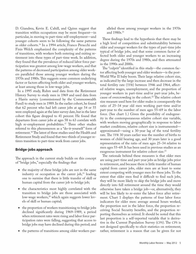
wage that he could earn in that bridge job to the wage he has been earning in a full-time career job at ages 50–54. For men in the 55–61, 62–64 and 65–69 age groups, the ratio fell from 1.29, 1.38 and 1.18 in 1967 to 0.80, 0.92, and 0.85 at some time during the 1984–1987 period, re-spectively. It then recovered to 1.12, 1.00 and 1.11 in the 2001–2004 period, presumably as baby boomers moved on and the market for part-year, part-time jobs eased. Table 1 and chart 3 demonstrate the close inverse cor-respondence between the number of younger men work-ing part year and/or part time, and these relative wages. The correspondence is weaker for men ages 62–64 (whose adjusted R-square is 0.41), but is considerably stronger for those ages 55–61 and 65–69 (with adjusted R-squares of 0.54 and 0.65, respectively). The table demonstrates the close correspondence between observed and predicted values, using just the number of younger part-year, part-time workers as an explanatory variable.

Data and methodology

The data used in this analysis has been drawn exclusively from Current Population Survey (CPS) Annual Social and Economic Supplement data for 1968–2009, as prepared

in uniform files in CPS Utilities by Unicon.24 Data covered all men ages 25–34 and 55–69, with the 25–34 age group used for the numerator of a relative cohort size variable, and men ages 55–69 in the labor force for the remainder of the analyses.25

The methodology employed is that of a typical labor supply model, but with relative cohort size variables add-ed. The relative cohort size variable used was calculated as the number of 25–34 year old men working part year and/or part time relative to the number of men in the la-bor force ages 55–69 in each year and state.26 Age-specific unemployment rates were calculated for each of the three groups—age 55–61, 62–64 and 65–69—calculated at the Metropolitan Statistical Area (MSA) level,27 and regres-sions were run using individual-level micro data with these state- and MSA-level variables attached to each re-cord. In addition, each age-group’s model was also tested with a 30-year lag of the total fertility rate as an instru-ment for the relative cohort size measure. Summary sta-tistics describing the data are presented in appendix tables A-1 through A-3.

Four models were estimated for four labor supply indicators, separately for each of the three age groups. (See box.)

Equations for labor supply models

0 1 2 3 4 5 6ln (1)e o State MSAH W I I RCS U M X uβ β β β β β β ′= + + + + + + +Β +

0 1 2 3 4 5 6ln ' (2)e o State MSAOLF W I I RCS U M X uγ γ γ γ γ γ γ= + + + + + + +Γ +

0 1 2 3 4 5 6ln ' (3)e o State MSAR W I I RCS U M X uα α α α α α α= + + + + + + + Α + 0 1 2 3 4 5 6ln ' (4)SS e o State MSAR W I I RCS U M X uδ δ δ δ δ δ δ= + + + + + + + ∆ +

where

H represents annual hours worked in the previous year (including those with zeroes); OLF represents a binary variable set to 1 for those out of the labor force;R represents a binary variable set to 1 for those identifying themselves as retired.28

SSR represents a binary variable set to 1 for those receiving Social Security benefits;W represents the man’s own (instrumented) hourly wage, in constant 2008 dollars;

eI represents the earnings of others in the family, defined as total family earnings minus own earnings, in constant 2008 dollars;

oI represents other income, which comprises interest, dividends, and rent, in 2008 dollars;

StateRCS represents the year- and state-specific relative cohort size;

MSAU represents the age- and MSA-specific unemployment rate, in the year prior to the survey; M represents a binary variable set to 1 for those who are married with spouse present; andX is a vector of control variables.


The control variables included single-year age dummies, 4

education dummies (with 16 years as the reference group), 3 race dummies (with non-Hispanic Whites as reference group), 20 state dummies,29 a time trend, and 3 indicators of MSA status (principal city, balance of MSA, and non-MSA).

In addition, each of the models (1)–(4) was estimated for each age group, substituting a 30-year lag of the total fertility rate for the potentially endogenous relative cohort size variable. RCS could be endogenous, especially at the state level, if individuals move in response to changes in economic conditions. The lagged TFR, in contrast, is com-pletely exogenous because it was determined 30 years ear-lier. And as previously explained, since the TFR represents the number of births relative to the number of women of childbearing age, a 30-year lag of the TFR will approxi-mate the number of individuals ages 25–34 relative to those ages 55–69.

Finally, the models for those ages 62–64 and 65–69 were estimated with controls for the major changes in Social Security and age discrimination that occurred during the study period. For both age groups, these controls included a variable representing the changing levels of the age-spe-cific earnings threshold imposed on the receipt of Social Security benefits. These thresholds are illustrated in chart 4. In addition, for those aged 65–69 the controls included•a dummy for the years after 1990, the period in which

the delayed retirement credit was increased;•another for the period after 2000, when the Senior

Citizens’ Freedom to Work Act was passed, removing the earnings threshold for those ages 65–69; and

•two dummies, one for the years following 1978 and another for the years following 1986, when the Age Discrimination in Employment Act was implemented.

The methodology comprised three steps. In the first, hourly wages were calculated—in 2008 dollars, using the Con-sumer Price Index—as total annual wages and salary in

the previous year divided by annual hours worked, with the latter calculated as weeks worked times the usual number of hours worked per week in the previous year.30 The annual wages and salary were first multiplied by a fac-tor of 1.45 if topcoded.31 The hourly wage was imputed for those with no reported wage, as well as for the self-employed and those whose calculated wage fell outside the range of $2.50—$250 in 2008 dollars. The imputa-tion process was based on separate regressions of the nat-ural logarithm of wages (logwage) for those with fewer than 20 weeks worked and those with 20 or more weeks worked, separately for each age group. That is, it was as-sumed that wages should be imputed on the basis of the reported wage of those in groups with similar numbers of weeks worked.32

The imputation regressions were run separately in each of 14 groupings, with each grouping including 3 ages (for example, 55–57, 56–58, etc.). The 3-year groupings were used to achieve larger sample sizes for the imputation process, and the CPS March Supplement Weights were normalized to sum to 1 in each year, so that each year carried equal weight in the regressions. The regressions each included 4 age dummies, 2 year dummies, 4 educa-tion dummies, 3 race dummies, 20 state dummies, and 3 indicators of MSA status.

Then in the second step, because observed wages are en-dogenous—they depend on a worker’s occupation, indus-try, and hours worked—wages were instrumented. This was again done separately for each age group and time period by regressing logwage on 4 age dummies, 4 educa-tion dummies, 3 race dummies, 20 state dummies, and 3 indicators of MSA status. In addition, a series of dummy variables representing wage deciles was included, which served as excluded instruments in the final hours, partici-pation, and retirement equations. As indicated in a 2007 study by Francine D. Blau and Lawrence M. Kahn, use of deciles “corrects to some degree for measurement error in the wage.”33

Table 1. Results of regressing the relative wage of older men on the number of men ages 25–34 working part year and/or part time

Men ages 55–61 Men ages 62–64 Men ages 65–69

Number of men ages 25–34 working part year and/or part time

–0.087(–7.26)

–0.073(–5.62)

–0.108(–9.26)

Adjusted R-square .5350 .4050 .6534Number of observations 46 46 46

NOTES: All t-statistics are in parentheses. The relative wage is defined here as the average wage of part-year and/or part-time workers relative to the average full-time wage of the previous 5-year age group. That is, the as-sumption is that a worker, in deciding whether to take a bridge job at ages

55–59, will compare the wage that he could earn in that bridge job relative to the wage he has been earning in a full-time career job, at ages 50–54.

SOURCES: Current Population Survey Annual Social and Economic Sup-plement and author’s calculations.



The third step involved estimating each of the equations in (1)–(4) separately for each age group, over the entire 42-year period. Equation (1) was treated as a weighted instrumental variable (IV) linear model, while equations (2), (3), and (4) were weighted IV binary probit models.

Results

The results of this procedure are presented in tables 2 and 3 for each of the three age groups, 55–61, 62–64 and 65–69. Table 2 presents more complete results for annual hours worked, using standardized coefficients in order to see the relative strengths of the different variables. Table 3 pres-ents just the estimated (marginal) effects of the relative cohort size and total fertility rate variables for the three “retirement” variables: the propensity to be out of the la-bor force, the propensity to report oneself as retired,34 and the propensity to claim Social Security benefits.

In all cases, the coefficients on the RCS and TFR variables display the expected signs and all are highly significant. The variables have a strong negative effect on hours worked and positive effects on the probability of being out of the labor force, reporting themselves as retired, and claiming Social Security benefits. This is consistent with the hypothesis that overcrowding in the market for part-year and part-time jobs induces older men to reduce their labor force participation; that is, the competition for part-year and/or part-time jobs leads men to skip bridge jobs and move directly out of the labor force from career jobs.

The strength of the estimated effects varies across age groups and across the four variables. For the 65–69 age group, the effects are strongest on hours worked, with elasticities of –.371 (for RCS) and –.717 (for TFR), although these elasticities are reduced somewhat, to –.232 (for RCS) and –.640 (for TFR), when the Social Security Administration controls are added in. For the

Chart 3. Relative hourly wages of men ages 55–69

1.5

1.4

1.3

1.2

1.1

1.0

.9

.8

1.5

1.4

1.3

1.2

1.1

1.0

.9

.8

Men ages 62–64

1960 1970 1980 1990 2000 2010

Relative wage Predicted values

1.5

1.4

1.3

1.2

1.1

1.0

.9

.8

1.5

1.4

1.3

1.2

1.1

1.0

.9

.81960 1970 1980 1990 2000 2010

Men ages 55–61


Relativewage

Relativewage

Relativewage

Relativewage

1.5

1.4

1.3

1.2

1.1

1.0

.9

.8

1.5

1.4

1.3

1.2

1.1

1.0

.9

.8

Men ages 65–69


1960 1970 1980 1990 2000 2010

Relativewage

Relativewage



55–61 age group, the estimated effects are strongest for the likelihood of reporting oneself as retired: .373 (for RCS) and .802 (for TFR). For those ages 62–64, the effects are very strong for both the propensity to report oneself as retired, with elasticities of .396 for the RCS and .833 for the TFR, and the propensity to claim Social Security benefits, .327 for the RCS and .677 for the TFR. (These effects on reporting oneself as retired and claiming Social Security benefits were both after controlling for the Social Security earnings threshold; the effects are actually increased by adding this control.) Overall, the effects of the two cohort size variables are actually strongest for the 62–64 age group. The weakest estimated elasticities were for hours worked among those in the 55–61 age group

(–.09 for RCS and –.15 for TFR).The estimated effect of the earnings threshold is not sig-

nificant for any of the four variables for the 62–64 age group,35 but the earnings threshold exerted a negative ef-fect on hours worked for the 65–69 age group (with a corresponding positive effect of the Freedom to Work Act after 2000). In the case of the other three variables for those ages 65–69, the threshold has a statistically signifi-cant positive effect only for the propensity to report one-self as retired, but only with the RCS—not with the TFR. Of the four dummy variables for those ages 65–69, only that for the Freedom to Work Act has consistently signifi-cant effects; the effects are positive for hours worked and negative for the other three variables.

Table 2. Independent variable regression results for annual hours worked (including zeroes, standardized coefficients)

Value Men ages 55–61 Men ages 62–64 Men ages 65–69

Lagged total fertilityrate

–.059(–23.3)

——

–.113(–27.7)

——

–.112(–27.0)

——

–.106(–30.6)

——

–.094(–14.1)

——

Relative cohort size(state-year specific)

——

–.072(–26.6)

——

–.114(–26.5)

——

–.113(–25.9)

——

–.100(–28.1)

——

–.063(–13.5)

Logwage .088(28.9)

.087(28.6)

.010(2.3)

.008(1.7)

.010(2.3)

.008(1.7)

–.055(–15.3)

–.058(–16.1)

–.057(–15.4)

–.059(–15.8)

Others' earnings (thousands)

.107(40.4)

.107(40.1)

.162(29.7)

.161(29.7)

.162(29.7)

.161(29.7)

.198(36.4)

.199(36.5)

.198(36.4)

.198(36.4)

Other income (thousands)

–.017(–5.8)

–.018(–6.1)

–.023(–5.2)

–.027(–6.0)

–.023(–5.2)

–.027(–6.0)

.007(1.7)

.003(0.6)

.007(1.8)

.006(1.4)

Married? .116(40.8)

.117(41.0)

.074(17.8)

.074(17.8)

.074(17.8)

.074(17.8)

.025(7.4)

.025(7.5)

.025(7.4)

.026(7.5)

Time trend –.149(–55.4)

–.130(–50.9)

–.225(–50.8)

–.188(–44.3)

–.235(–16.3)

–.191(–13.0)

–.151(–37.5)

–.116(–30.5)

–.259(–18.4)

–.230(–16.4)

SSA earnings threshold ——

——

——

——

.010(0.7)

.003(0.2)

——

——

–.016(–2.4)

–.036(–5.3)

Delayed retirementbenefit 1990?

——

——

——

——

——

——

——

——

.008(1.0)

.046(6.5)

Freedom to Work Act 2000?

——

——

——

——

——

——

——

——

.042(4.3)

.048(4.9)

Age discrimination in employment 1978?

——

——

——

——

——

——

——

——

.035(4.6)

.013(1.9)

Age discrimination in employment 1986?

——

——

——

——

——

——

——

——

.049(6.9)

.022(3.2)

Adjusted R-square .1148 .1156 .1258 .1244 .1258 .1244 .1177 .1160 .1186 .1181

TFR elasticity –.152 — –.465 — –.463 — –.717 — –.640 —

Relative cohort size elasticity — –.101 — –.254 — –.254 — –.371 — –.232

Number of observa-tions 207,478 201,147 74,156 73,971 74,156 73,971 106,870 106,550 106,870 106,550

NOTES: Reported hours worked are for years 1967–2008. Standardized coefficients and t-statistics are in parentheses. All regressions included 20 dummies for state groupings, age dummies, 4 education dummies, 3 race dummies, an MSA-specific unemployment rate, and 3 indicators of MSA resi-

dency status. Dash indicates not applicable.




Table 3. Independent variable binary probit estimated coefficients on relative cohort size measures for three retirement indicators (marginal effects)

ValueMen ages 55–61 Men ages 62–64 Men ages 65–69

Without SSA controls With SSA controls Without SSA controls With SSA controls

Not in the labor forceLagged total fertility rate 0.034 0.095 0.095 0.064 0.052

(19.4) (26.4) (25.8) (23.5) (9.7)[.424] [.550] [.546] [.251] [.204]

Relative cohort size (state-year specific) .130 .306 .307 .215 .148(23.6) (26.1) (25.7) (23.6) (12.3)[.286] [.309] [.310] [.148] [.102]

Retired (as self-reported)1

Lagged total fertility rate 0.021 0.075 0.076 0.079 0.059(21.1) (24.8) (24.6) (26.2) (9.8)[.802] [.732] [.833] [.429] [.317]

Relative cohort size (state-year specific) .055 .202 .204 .226 .117(18.8) (21.3) (21.1) (23.1) (9.0)[.373] [.392] [.396] [.216] [.112]

Claiming Social Security benefits

Lagged total fertility rate — 0.104 0.105 0.05 0.065— (29.1) (28.7) (21.9) (14.7)— [.673] [.677] [.168] [.219]

Relative cohort size (state-year specific) — .287 .288 .133 .098— (24.8) (24.4) (17.5) (9.8)— [.326] [.327] [.079] [.058]

1 Represents a binary variable set to 1 for those identifying themselves as retired. This is a self-reported variable, and is derivative in the CPS. That is, the CPS is not designed specifically to elicit statistics on retirement; rather, retirement is a reason that can be given for not having worked in the previ-ous year.

NOTES: Regarding marginal effects, t-statistics are in parentheses, and

elasticities are in brackets. All regressions included the variables displayed in table 1 plus 20 dummies for state groupings, age dummies, 4 education dummies, 3 race dummies, an MSA-specific unemployment rate, and 3 indi-cators of MSA residency status. Dash indicates not applicable.

SOURCES: Current Population Survey Annual Social and Economic Supple-ment and author’s calculations.

In terms of own-wage elasticities, there is a marked dif-ference across age groups. For hours worked, the effect is strongly positive for those ages 55–61, barely significant for those ages 62–64, and strongly negative for those ages 65–69, as shown on table 2. Conversely, in results available from the author, the effect on the propensity to be out of the labor force, and to report oneself as retired, is strongly negative for those ages 55–61, not significant for those ages 62–64, and strongly positive for those ages 65–69. There is a consistent, strongly negative effect in the older age groups for the propensity to claim Social Security benefits.

Marriage has consistent strong effects across all three age groups for hours worked (positive) and propensity to be out of the labor force (negative). In terms of the propen-sity to report oneself as retired, the effect for the two older age groups is not significant, and it is only barely negative-ly significant for the 55–61 age group. For claiming Social Security benefits, the effect is strongly negative for those ages 62–64, and strongly positive for those ages 65–69. The effect of “others’ earnings,” presumably in most cases a wife’s earnings, is consistently and significantly positive for hours worked for all age groups, and is negative for the

three retirement indicators. These two effects—the effect of marriage generally and of a wife’s employment—sug-gest support for the hypothesis that men tend not to retire when their wives are still in the labor force.

As might be expected, other income, including such items as interest, rent, and dividends, has a negative ef-fect on hours worked and a positive effect on the other three variables for the two younger age groups. For those ages 65–69, however, the effects are only significant for the two retirement variables. The effect of the time trend is strongly negative on hours worked and positive on the other three indicators, even after controlling for other variables.

Table 4 is an attempt to estimate the real-world signifi-cance of the relative cohort size variables. The table in-dicates the maximum positive and negative changes that occurred in each of the four variables for each age group (using the means reported in appendix tables A-1 through A-3), and then estimates the percentage of those changes that might be attributed to changes in the two relative cohort size variables, using the estimated marginal effects of the RCS variables. In the case of annual hours worked,


the decreases occurred in the first half of the study period, while the increases occurred in the second half of the pe-riod. The opposite is true for the other three variables.

Overall, the effects seem to be most realistic for the first half of the period, when hours worked were declining and the other three variables were increasing. In that period, each of the RCS and TFR variables is estimated to account for an average of about 29 percent of the observed chang-es over all four variables and three age groups. The lowest proportions were for those reporting themselves as retired, where each of the two cohort size variables accounted for about 22 percent of the observed changes.

In general, the two variables overpredict changes in the second half of the period, when hours worked were in-creasing and the other three variables were decreasing. On average, the RCS explains 124 percent of the changes in the second half of the period, while the TFR explains 171 percent of the observed changes in that period. However, looking just at the two older age groups, the RCS explains an average of 80 percent of the observed second-half changes, while the TFR explains 138 percent. Excluding

the proportion reporting themselves as retired, for the two older age groups in the second half of the period, the RCS explains 72 percent of the observed changes, while the TFR explains 120 percent of the observed changes. This tendency to overpredict in the second half of the period could be the effect of a “stickiness” in behavior once the pattern of earlier retirement had been set by the earlier cohorts.

Recapping the results in table 4, for the two older age groups, the RCS appears to provide the most realistic esti-mates, as it predicts 29 percent of the changes in the first half of the period and 80 percent of the changes in the second half of the period.

Finally, table 5 looks at the potential explanatory power of the relative cohort size variables for men with lower levels of education—that is, fewer than thirteen years, or at most a high school education. The hypothesis in esti-mating these effects was that, if bridge jobs are generally lower-skilled jobs, then men with lower levels of educa-tion would be more likely to move into them. Thus the competition with younger workers might be greater for

25,000

20,000

15,000

10,000

5,000

0

Chart 4. Social Security earnings thresholds for workers ages 62–64 and 65–69

25,000

20,000

15,000

10,000

5,000

01968 1974 1980 1986 1992 1998 2004 2010

Ages 62–64

Year

SOURCE: Social Security Administration, “Annual Statistical Supplement 2010, table 2.A29.

Earnings(2008 dollars)

Earnings(2008 dollars)

Ages 65–69



this group. In addition, this group might be less likely to have adequate savings or pensions for support in retire-ment, and therefore might be more likely to move into bridge jobs rather than directly into retirement.

Table 5 is based on separate regressions, not shown here, but available from the author on request. The averages and proportions observed over the years for those with lower levels of education are reported in appendix table A-4. Us-ing both the marginal effects in the estimated equations and the observed changes in the relative cohort size vari-ables, table 5 attempts to explain the changes observed in

table A-4. In general, the explanatory power of the relative cohort size variables is better for this group, with changes in the RCS explaining about 37 percent of the changes in the first half of the period (compared with 29 percent for men at all levels of education) and 92 percent in the sec-ond half of the period (compared with 124 percent for all men). Changes in the TFR explain about 34 percent in the first half (compared with 29 percent for all men) and 192 percent in the second half (compared with 171 percent for all men). The best explanatory power for this education group occurs with the RCS for the two older age groups, in

1 Represents a binary variable set to 1 for those identifying themselves as retired in a CPS question about why they did not work in the previous year.

NOTES: This table uses the averages and proportions reported in tables A-1 through A-3 and estimated marginal effects from the regressions re-ported in tables 2 and 3. For men ages 62–64 and 65–69, the marginals

used are those estimated in equations controlling for the various changes in Social Security regulations. The estimated effects are larger when these changes are not controlled for. Dash indicates not applicable.


Table 4. Potential explanatory power of the relative cohort size variables for men ages 55–69

CategoryMen ages 55–61 Men ages 62–64 Men ages 65–69

Max increase Max decrease Max increase Max decrease Max increase Max decrease

Average annual hours worked 63.3 305.3 183.8 664.2 184.0 393.8 Percent explained by changes in RCS 169.3 37.3 100.0 29.4 54.6 26.9 Percent explained by changes in TFR 167.3 20.9 119.6 19.9 128.9 44.7

Proportion not in the labor force .133 .010 .268 .091 .164 .097 Percent explained by changes in RCS 31.1 390.0 36.6 101.0 33.8 54.2 Percent explained by changes in TFR 17.3 380.0 23.9 116.6 40.8 92.8

Proportion reporting themselves as retired1 .080 .010 .242 .055 .243 .044 Percent explained by changes in RCS 21.9 170.0 26.8 110.9 18.0 94.4 Percent explained by changes in TFR 17.2 230.0 21.1 153.1 30.9 229.7

Proportion claiming Social Security benefits — — .247 .123 .147 .067 Percent explained by changes in RCS — — 37.2 70.0 24.9 51.9 Percent explained by changes in TFR — — 28.4 94.9 56.9 168.2

Table 5. Potential explanatory power of the relative cohort size variables for men ages 55–69 with fewer than 13 years of education

CategoryMen ages 55–61 Men ages 62–64 Men ages 65–69

Max increase Max decrease Max increase Max decrease Max increase Max decrease

Average annual hours worked 61.9 417.5 162.6 756.8 152.4 420.6 Percent explained by changes in RCS 183.6 28.9 116.6 26.6 57.2 22.0 Percent explained by changes in TFR 278.2 31.1 229.1 37.1 175.3 47.9

Proportion not in the labor force .146 0 .198 .080 .074 .069 Percent explained by changes in RCS 32.4 (2) 49.8 115.9 66.2 66.7 Percent explained by changes in TFR 33.4 — 66.1 217.1 91.4 130.0

Proportion reporting themselves as retired1 .080 .022 .242 .068 .261 .071 Percent explained by changes in RCS 25.0 90.9 30.3 101.7 18.1 63.0 Percent explained by changes in TFR 39.2 189.1 46.6 219.7 30.4 150.4

Proportion claiming Social Security benefits — — .289 .113 .149 .073 Percent explained by changes in RCS — — 33.8 81.2 74.1 41.8 Percent explained by changes in TFR — — 52.3 177.4 54.9 151.0

1 Represents a binary variable set to 1 for those identifying themselves as retired in a CPS question about why they did not work in the previous year.

2 The proportion of men ages 55–61 with less education who were not in the labor force continued increasing after 1990.

NOTES: This table uses the averages and proportions reported in table A-4 and estimated marginal effects which are available upon request from

the author. For men ages 62–64 and 65–69, the marginals used are those estimated in equations controlling for the various changes in Social Secu-rity regulations. The estimated effects are larger when these effects are not controlled for. Dash indicates not applicable.



this case for the proportion out of the labor force (58 per-cent in the first half and 91 percent in the second) and the proportion claiming Social Security benefits (54 percent in the first half and 62 percent in the second.)

THIS STUDY HAS MADE USE of a measure of relative co-hort size: the number of 25–34 year old men working part year and/or part time relative to the number of 55–69 year old men in the labor force. For purposes of analysis, the measure was calculated, using March Current Population Survey (CPS) data, for each man at the level of his state. This relative cohort size measure might be thought of as a direct function of a 30-year lag of the total fertility rate, a measure often used to illustrate the effects of the post-World War II baby boom. This correspondence relates to the fact that the TFR indicates the number of children per woman of childbearing age, so that a 30-year lag can be thought of as an exogenous representation of the ratio of 25–34 year olds relative to 55–69 year olds.

More importantly, the relative cohort size measure has been shown here to be a highly significant factor—both statistically and substantively—affecting older men’s an-nual hours worked, labor force participation, propensity to report themselves as retired, and propensity to claim Social Security benefits. In general terms, relative cohort size can be said to have generated about 29 percent of the observed changes in these variables in the period up to about 1990. The variable does, however, somewhat over-predict observed changes in the period since 1990, with the ratio of 25–34 year old part-time workers relative to 55–69 year olds in the labor force overpredicting by 24 percent the observed changes in these four variables in the later period.

For men with at most a high school education—such men are most likely to work in bridge jobs—the explana-tory power of the relative cohort size variable is some-what better, explaining about 37 percent of changes in the early period and 92 percent in the second. The explanatory power is best for men in the age groups 62–64 and 65–69; for the proportion out of the labor force and proportion claiming Social Security benefits among these age groups, the RCS variable explains on average 56 percent of chang-es in the first part of the study period and 76 percent in the second period.

However, a significant portion of the sharp decline in annual hours worked and labor force participation in the 1970s remains unexplained, indicating the considerable role played by the other factors that have been identified as important in affecting older men’s decision to retire: access to health insurance, and changes in Social Security and pensions.

We have begun to experience the entry of the “echo boom” into the labor market, and one might initially ex-pect that this would once again tend to motivate older workers to retire at higher rates as the echo boom moves into its twenties and thirties. However, the ratio of these young workers to older workers will remain low because the older workers will themselves be members of the large baby boom cohort. Hence, it remains to be seen whether it is the absolute or the relative size of the younger co-hort which is significant in affecting patterns in the older cohort, or whether the large size of the retiring cohort itself may affect its labor force participation patterns. Any attempt to tease out the effects will have to differentiate them from the effects of the recent recession and diminu-tion of 401(k)s.

NOTES

1 Diane J. Macunovich, “The Fortunes of One’s Birth: Relative Cohort Size and the Youth Labor Market in the U.S.,” Journal of Population Economics, June 1999, pp. 215–272 and Birth Quake: The Baby Boom and Its Aftershocks (Chicago: University of Chicago Press, 2002).

2 Joseph F. Quinn, Retirement Trends and Patterns in the 1990s: The End of an Era? Boston College Working Papers In Economics, no. 385, 1997; New Paths to Retirement, no. 406, 1998; and Has the Early Retirement Trend Reversed? no. 424, 1999.

3 Gary Englehart and Anil Kumar, “The Repeal of the Retirement Earnings Test and the Labor Supply of Older Men,” Journal of Pension Economics and Finance, October 2009, pp. 429–450.

4 David A. Wise, “Social Security Provisions and the Labor Force Participation of Older Workers,” Population and Development Review, supplement to vol. 30, 2004, pp. 176–205.

5 Alan Krueger and Jörn-Steffen Pischke, “The Effect of Social Security on Labor Supply: A Cohort Analysis of the Notch Generation,” Journal of Labor Economics, University of Chicago Press, October 1992, pp. 412–437.

6 Patricia M. Anderson, Alan L. Gustman, and Thomas L. Steinmeier, “Trends in Male Labor Force Participation and Retirement: Some Evidence on the Role of Pensions and Social Security in the 1970s and 1980s,” Journal of Labor Economics, University of Chicago Press, October 1999, pp. 757–783.

7 Leora Friedberg and Anthony Webb, “Retirement and the Evolution of the Pension Structure,” The Journal of Human Resources, Spring 2005, pp. 281–308.

8 Courtney C. Coile and Phillip P. Levine, “Bulls, Bears and Retirement Behavior,” Industrial and Labor Relations Review, Cornell University, April 2006, pp. 408–429.

http://ideas.repec.org/a/ucp/jlabec/v17y1999i4p757-83.html



http://ideas.repec.org/s/ucp/jlabec.html



9 Lynn A. Karoly and Jeannette A. Rogowski, “The Effects of Access to Post-Retirement Health Insurance on the Decision to Retire Early,” Industrial and Labor Relations Review, October 1994, pp. 103–123.

10 David M. Blau and Donna B.Gilleskie, “Retiree Health Insurance and the Labor Force Behavior of Older Men in the 1990s,” The Review of Economics and Statistics, February 2001, pp. 64–80.

11 Richard W. Johnson, Amy J. Davidoff, and Kevin Perese, “Health Insurance Costs and Early Retirement Decisions,” Industrial and Labor Relations Review, Cornell University, July 2003, pp. 716–729.

12 Dan A. Black and Xiaoli B. Liang, “Local Labor Market Conditions and Retirement Behavior,” Working Paper 2005–08, Center for Retirement Research at Boston College, May 2005.

13 Alicia H. Munnell, Mauricio Soto, Robert K. Triest, and Natalia A. Zhivan, How Much Do State Economics and Other Characteristics Affect Retirement Behavior? Working Paper 2008–12, Center for Retirement Research at Boston College, 2008.

14 The average income of men ages 45–54 increased between 1970 and 2010 by only 2.5 percent in real terms. Over a 40-year timespan, we would expect improvements in productivity to lead to more growth than this.

15 Kevin E. Cahill, Michael D. Giandrea, and Joseph F. Quinn, “Re-entering the labor force after retirement,” Monthly Labor Review, June 2011, pp. 34–41.

16 Michael D. Giandrea, Kevin E. Cahill, and Joseph F. Quinn, Self-Employment Transitions Among Older American Workers with Career Jobs, Boston College Working Papers in Economics, no. 684, 2008; and Bridge Jobs: A Comparison Across Cohorts, Boston College Working Papers in Economics, no. 670, 2008.

17 Christopher J. Ruhm, “Secular changes in the work and retire-ment patterns of older men,” The Journal of Human Resources, Spring 1995, pp. 362–385.

18 Quinn, New Paths to Retirement and Has the Early Retirement Trend Reversed? Giandria et al., A Micro-Level Analysis of Recent Trends in Labor Force Participation among Older Workers, Working Paper 2008–08, Center for Retirement Research at Boston College, 2008.

19 Christopher J. Ruhm, “Bridge jobs and partial retirement,” Jour-nal of Labor Economics, University of Chicago Press, October 1990, pp. 482–501.

20 Franco Peracchi and Finis Welch, “Trends in labor force transi-tions of older men and women,” Journal of Labor Economics, April 1994, pp. 210–242.

21 Peracchi and Welch, “Trends in labor force transitions.”22 Macunovich, “The Fortunes of One’s Birth” and Birth Quake.23 See Macunovich, “The Fortunes of One’s Birth.”24 Data used from Unicon Corporation’s CPS utilities were for the

years 1968–2009. 25 Those in the military were excluded from the analysis, however.26 There were 51 separate jurisdictions (50 states and the District of

Columbia) identified from 1977 to 2009, 22 from 1973 to 1976, and 30 from 1968 to 1972.

27 MSA was not available prior to 1977, so state-level variables were used, specific to each age group, for those years. After 2004, BLS changed from MSAs to Consolidated Statistical Areas (CSA). The re-sulting number of levels used in each year was 21 for 1969–1976, 45 for 1977–1985, 248 for 1986–2004, 281 for 2005, and 265 for 2006–2009. For those not living in an MSA, the state-level variable was used.

28 As noted previously, the binary variable “retired” is a self-reported variable that is is derivative in the CPS. The CPS is not designed specifi-cally to elicit statistics on retirement; rather, retirement is a reason that can be given for not having worked in the previous year.

29 There were 21 state groupings that were consistently available dur-ing all 42 years.

30 Because the variable “hours worked per week in the previous year” was not available prior to 1976 and weeks worked in the previous year were available only in groupings, an imputation algorithm developed by Finis Welch in 1979 was used to allocate hours and weeks worked for these years. Details are available from the author upon request. Also, see Finis Welch, “Effects of Cohort Size on Earnings: The Baby Boom Babies’ Financial Bust,” Journal of Political Economy, The Univer-sity of Chicago Press, October 1979, pp. S65–S97.

31 This technique was used by Francine D. Blau and Lawrence M. Kahn in “Changes in the Labor Supply Behavior of Married Women, 1980–2000,” Journal of Labor Economics, University of Chicago Press, July 2007, pp. 393–438.

32 The same technique was used in Blau and Kahn, “Changes in the Labor Supply Behavior.”

33 Blau and Kahn, “Changes in the Labor Supply Behavior,” p. 406.34 See endnote 26.35 The detailed regression results for the three variables reported in

table 3 are available from the author upon request.


Table A–1. Summary statistics for men ages 55–61

Category 1969–1971 1974–1976 1979–1981 1984–1986 1989–1991 1994–1996 1999–2001 2007–2009 1968–2009Average annual hours worked1 1,942.9 1,795.9 1,732.9 1626.0 1,637.6 1,606.7 1,670.0 1,636.6 1,704.7Proportion not in the labor force .124 .176 .211 .243 .241 .257 .255 .247 .219Proportion retired2 .018 .035 .056 .085 .091 .096 .098 .086 .071Relative cohort size3 .295 .422 .559 .669 .624 .613 .364 .314 .498Lagged total fertility rate 2.236 2.588 3.085 3.519 3.600 2.906 2.366 1.791 2.731Unemployment rate .033 .043 .035 .054 .048 .048 .033 .050 .044Logwage 2.924 3.021 3.100 3.070 3.061 3.056 3.097 3.079 3.063Other’s earnings4 21,074 20,862 22,394 22,470 26,083 25,785 29,767 31,242 25,653Other income5 — — 4,830 6,467 6,783 6,204 7,405 5,310 4,743Proportion married .867 .828 .828 .819 .792 .786 .748 .715 .798Fewer than 12 years of school .548 .446 .368 .343 .268 .203 .144 .104 .29512 years of school .265 .335 .334 .335 .363 .341 .333 .294 .32213–15 years of school .086 .101 .125 .119 .139 .204 .224 .267 .16316 years of school .053 .065 .098 .106 .108 .141 .159 .199 .119More than 16 years of school .048 .053 .075 .097 .122 .111 .140 .136 .101Black .026 .077 .083 .090 .093 .091 .088 .097 .081Hispanic .008 .025 .033 .045 .060 .065 .075 .087 .051Other .003 .011 .015 .019 .025 .032 .042 .054 .026Sample size 13,973 12,467 16,566 14,960 13,212 11,682 11,901 22,463 209,436

1 Includes those with 0 hours. Hours were imputed for years before 1976 using the algorithm from Finis Welch, “Effects of Cohort Size on Earnings: The Baby Boom Babies’ Financial Bust,” Journal of Political Economy, October 1979.

2 As self-reported: reason given for not working.3 Number of men ages 25–34 working part time and/or part year divided

by number of men in the labor force ages 55–69.4 Total family earnings minus own earnings.5 Interest, dividends, and rent. Data not available in first two periods.SOURCES: Current Population Survey Annual Social and Economic

Supplement and author’s calculations.


Category 1969–1971 1974–1976 1979–1981 1984–1986 1989–1991 1994–1996 1999–2001 2007–2009 1968–2009Average annual hoursworked1 1,611.3 1,355.6 1,212.6 1,044.8 995.1 947.1 1,040.0 1,130.9 1,163.0Proportion not in labor force .295 .411 .464 .533 .548 .563 .523 .472 .472Proportion retired2 .093 .135 .204 .284 .317 .335 .309 .280 .280Proportion claiming Social Security benefits .253 .371 .429 .476 .491 .500 .469 .377 .422Relative cohort size3 .295 .422 .559 .669 .624 .613 .364 .314 .498Lagged total fertility rate 2.236 2.588 3.085 3.519 3.600 2.906 2.366 1.791 2.731Unemployment rate .028 .048 .039 .051 .041 .050 .033 .048 .043Logwage 2.882 2.941 3.011 3.004 3.076 2.855 3.007 3.123 3.001Others’ earnings4 17,878 17,791 18,759 17,730 20,477 19,739 25,078 26,483 20,763Other income5 — — 5,549 7,859 8,454 6,424 6,934 6,433 5,358Proportion married .831 .823 .824 .808 .805 .796 .774 .754 .801Fewer than 12 years of school .612 .543 .435 .368 .331 .242 .198 .116 .34712 years of school .210 .266 .322 .337 .322 .329 .334 .287 .30713-15 years of school .079 .091 .116 .117 .138 .190 .208 .248 .14816 years of school .099 .050 .071 .098 .113 .130 .141 .194 .107More than 16 years of school .049 .050 .056 .080 .096 .109 .119 .155 .091Black .025 .087 .081 .084 .089 .087 .085 .082 .078Hispanic .006 .025 .026 .042 .048 .061 .074 .078 .046Other .003 .008 .012 .020 .022 .022 .039 .048 .024Sample size 8,495 10,707 10,402 9,801 8,956 7,378 6,771 12,282 128,820


2 As self-reported: reason given for not working.3 Number of men ages 25–34 working part time and/or part year divided

by number of men in the labor force ages 55–69.4 Total family earnings minus own earnings.5 Interest, dividends, and rent. Data not available in first two periods.


APPENDIX: Supplementary tables



Table A–4. Labor force characteristics for men with fewer than 13 years of education

Category 1969–1971 1974–1976 1979–1981 1984–1986 1989–1991 1994–1996 1999–2001 2007–2009 1968–2009

Men ages 55–61

Annual hours worked 1,893.4 1,741.0 1,634.2 1,516.5 1,512.9 1,475.9 1,485.7 1,414.0 1,579.2

Proportion not in the labor force .134 .193 .244 .279 .280 .300 .319 .329 .262

Proportion reporting themselves as retired .017 .032 .060 .089 .097 .079 .089 .075 .067

Men ages 62–64

Annual hours worked 1,550.4 1,288.7 1,124.8 919.1 881.7 793.6 910.3 956.2 1,046.1


Proportion reporting themselves as retired .096 .134 .213 .302 .338 .324 .294 .270 .249

Proportion claiming Social Security benefits .275 .398 .470 .526 .545 .564 .529 .451 .473

Men ages 65–69

Annual hours worked 807.9 564.3 474.1 392.5 396.7 387.3 446.0 539.7 493.9


Proportion reportingthemselves as retired .323 .424 .489 .584 .581 .562 .546 .513 .511

Proportion claiming Social Security benefits .729 .824 .858 .878 .860 .870 .844 .805 .837



Category 1969–1971 1974–1976 1979–1981 1984–1986 1989–1991 1994–1996 1999–2001 2007–2009 1968–2009Average annual hours worked1 863.7 637.8 541.0 469.9 518.6 538.8 574.8 653.9 585.1Proportion not in the labor force .584 .676 .713 .748 .732 .727 .701 .651 .697Proportion retired2 .317 .414 .476 .562 .559 .560 .548 .516 .503Proportion receiving Social Security benefits .703 .794 .836 .850 .832 .841 .823 .783 .812Relative cohort size3 .295 .422 .559 .669 .624 .613 .364 .314 .498Lagged total fertility rate 2.236 2.588 3.085 3.519 3.600 2.906 2.366 1.791 2.731Unemployment rate .040 .062 .045 .042 .032 .035 .033 .051 .044Logwage 2.681 2.762 2.815 2.894 2.873 2.923 2.967 2.905 2.861Other’s earnings4 12,309 11,698 11,398 11,236 12,761 13,769 16,347 17,475 13,237Other income5 — — 7,166 9,589 10,223 7,818 10,279 8,287 6,914Proportion married .778 .814 .798 .796 .794 .777 .778 .767 .788Fewer than 12 years of school .696 .609 .544 .440 .377 .300 .237 .156 .40912 years of school .157 .207 .260 .326 .320 .324 .326 .339 .28713–15 years of school .056 .081 .089 .103 .125 .174 .199 .210 .13316 years of school .054 .058 .059 .064 .097 .116 .139 .154 .095More than 16 years of school .037 .045 .048 .067 .081 .086 .099 .141 .076Black .025 .089 .087 .080 .081 .078 .089 .081 .079Hispanic .006 .023 .028 .035 .045 .058 .067 .073 .042Other .003 .010 .015 .019 .027 .023 .039 .054 .025Sample size 6,524 8,877 8,537 7,990 7,736 6,503 5,540 9,110 106,870


2 As self-reported: reason given for not working.3 Number of men ages 25–34 working part time and/or part year divided by

number of men in the labor force ages 55–69.4 Total family earnings minus own earnings5 Interest, dividends, and rent. Data not available in first two periods.


Monthly Labor Review, May 2012: Older men: pushed into ... · PDF fileDuring the...

Documents

Transcript of Monthly Labor Review, May 2012: Older men: pushed into ... · PDF fileDuring the...