JHEP06(2014)048

Published for SISSA by Springer

Received: March 4, 2014

Accepted: May 19, 2014

Published: June 9, 2014

Monopoles and Wilson lines

David Tong and Kenny Wong

Department of Applied Mathematics and Theoretical Physics, University of Cambridge,

Wilberforce Road, Cambridge, CB3 0WA, U.K.

E-mail: d.tong@damtp.cam.ac.uk, k.wong@damtp.cam.ac.uk

Abstract: We present a semi-classical description of BPS monopoles interacting with

Wilson lines. The Wilson lines are represented as non-Abelian spin impurities. These spins

interact with the monopole degrees of freedom through a natural connection on the moduli

space. We employ this technology in N = 2 SU(2) gauge theory to count the number of

framed BPS states of a single monopole bound to Wilson lines in different representations.

Keywords: Supersymmetric gauge theory, Solitons Monopoles and Instantons

ArXiv ePrint: 1401.6167

Open Access, c© The Authors.

Article funded by SCOAP3.doi:10.1007/JHEP06(2014)048

JHEP06(2014)048

Contents

1 Introduction and results 1

2 Spin impurities and Wilson lines 2

2.1 Classical spin 2

2.2 Quantum spin 3

2.3 The path integral 4

3 Monopole dynamics 7

3.1 A review of monopoles 7

3.2 Moduli space dynamics 8

3.3 Monopoles and Wilson lines 10

3.4 Classical scattering 12

4 Quantum bound states 14

4.1 Supersymmetric dynamics 14

4.2 Quantum bound states 15

5 Future directions 20

1 Introduction and results

Magnetic monopoles are interesting. At weak coupling, they arise as solitons in non-Abelian

gauge theories [1, 2]. Tracing the fate of these monopoles to the strong coupling regime has

proven to be a fruitful technique to understand the dynamics, phase structure and duality

properties of quantum field theories.

The low-energy dynamics of BPS monopoles is best described using the moduli space

approximation [3]. The moduli spaceM is the space of solutions to the classical monopole

equations; it can be thought of as the configuration space of monopoles. The low-energy

dynamics is governed by a sigma-model with target spaceM, endowed with a natural metric

that is induced by the underlying gauge theory. This means that the classical scattering

of monopoles is described by geodesic motion on M while quantum states correspond to

functions or forms over M.

The purpose of this paper is to extend the moduli space description of monopole

dynamics to situations where there are also external quarks, sitting at fixed positions in

space. Such fixed quarks are usually represented by the insertion of a Wilson line operator

in the path integral,

WR[A0] = TrR P exp

(i

∫dtA0

)(1.1)

– 1 –

JHEP06(2014)048

Here R denotes some representation of the gauge group which, for the purposes of this

paper, we take to be SU(N). Wilson lines, and their supersymmetric generalisations, are

crucial to our understanding of quantum field theory, from their original role as order

parameters for confinement [4], to recent discussions, elucidating more subtle aspects of

gauge symmetry and supersymmetry [5, 6].

In order to describe the way monopoles interact with external quarks, it will prove

useful to work with a different description of the Wilson line. The starting point is a

simple, semi-classical model of an external quark, viewed as a fixed electric source for the

non-Abelian gauge field. Such a quark carries colour degrees of freedom, described by a

spin, or vector of fixed length, and the background gauge field causes this spin to precess.

It is straightforward to show that the quantum mechanical path integral for such a spin

is equal to the Wilson line: Zspin[A0] = WR[A0]. In other words, the Wilson line can be

thought of as the effect of integrating out localised spin degrees of freedom. We review this

perspective on the Wilson line in section 2.

The main result in this paper is contained in section 3 where we explain how magnetic

monopoles couple to the localised spins and, through this, to Wilson lines. As we shall

see, this too has an elegant geometrical description in the moduli space language. While

the underlying gauge dynamics induce a natural metric onM, it also provides the moduli

space with a number of further geometric quantities. Among these is an SU(N) gauge

connection. We will show that the electric degrees of freedom of the external quark couple

to this connection. As we will see, this leads to the expected non-Abelian Lorentz-force

law for the centre of mass motion of monopoles in the presence of an electric charge. But

it also leads to more subtle dynamics in which moving monopoles exchange electric charge

with fixed, external quarks.

Finally, in section 4, we use this approach to study the supersymmetric quantum

mechanics of monopoles in N = 2 SU(2) Yang-Mills. We compute some simple examples

of framed BPS states [5], involving quantum monopoles bound to Wilson lines in different

representations.

2 Spin impurities and Wilson lines

In this first section, we explain how spin impurities, coupled to bulk gauge fields, can

be thought of as Wilson lines. The essence of these ideas is not new. Early discussions

were given, for example, in [7, 8]. Mathematically, the relationship uses the framework of

geometric quantization and a readable exposition can be found in [9]. Here, however, we

take a different tack. Our goal is to describe the connection between Wilson lines and spin

impurities in a pedestrian manner without ever mentioning the words “nilpotent orbit”.

2.1 Classical spin

Classically, we view a spin as an N -component complex vector wa, a = 1, . . . , N of fixed

length,

w†w = κ (2.1)

– 2 –

JHEP06(2014)048

We further identify vectors which differ only by a phase: ωa ∼ eiθwa. This means that the

vectors parameterise the projective space CPN−1.

To implement the phase equivalence of vectors, we introduce an auxiliary U(1) gauge

field α which lives on the worldline of the spin. The action is

S =

∫dt(iw†Dtw − κα

)where Dt = ∂tw− iαw. There is now a gauge symmetry w → eiθ(t)w. Correspondingly, the

gauge field acts as a Lagrange multiplier, implementing the constraint (2.1). Note that κ

appears as a one-dimensional Chern-Simons term in the action and we will see below that

there is an associated quantisation condition on κ.

Importantly, because the action is first order, rather than second order, the classical

spin has a phase space, rather than configuration space, given by CPN−1. As we will

see shortly, upon quantisation this compact phase space results in a finite dimensional

Hilbert space. Actions of this kind are familiar from the discussion of classical spin-1/2

particles [10].

So far our spin has no dynamics. This arises by coupling it to a background SU(N)

gauge field Aµ. This gauge field propagates in d+ 1 spacetime dimensions and is governed

by its own equations of motion which we shall consider later in the paper. Meanwhile, the

spin impurity sits at a fixed position in space which we will take to be the origin. The

action for the spin is

Sspin =

∫dt(iw†Dtw − κα− w†A0(t)w

)(2.2)

where A0(t) = A0(~x = 0, t) is the value of the temporal gauge field at the origin. Physically,

we can think of this spin impurity as a classical quark. Although the position of the quark

is fixed at the origin, its gauge orientation is described by wa and is free to fluctuate. The

classical equations of motion now tell us that the background gauge field causes the spin

to precess. In α = 0 gauge, we have

idw

dt= A0(t)w

This has solution

w(t) = P exp

(i

∫ t

t0

dt′ A0(t′)

)w(t′)

where P stands for path ordering. We see that, already classically, the unitary operator

associated to the Wilson line plays a role in the dynamics of this system. However, our

real interest is in the quantum story.

2.2 Quantum spin

It is a simple matter to quantise the spin system. It is easiest to first work in the Hamil-

tonian formalism, starting with the unconstrained variables, wa. These obey the commu-

tation relations,

[wa, w†b ] = δab

– 3 –

JHEP06(2014)048

We define a “ground state” |0〉 such that wa|0〉 = 0 for all a = 1, . . . , N . A general state in

the Hilbert space then takes the form

|a1 . . . an〉 = w†a1. . . w†an |0〉

In the quantum theory, there is a normal ordering ambiguity in defining the constraint (2.1).

The symmetric choice is to take the charge operator

Q =1

2(w†awa + waw

†a) (2.3)

and to impose the constraint

Q = κ (2.4)

The spectrum of Q is quantised which means that the theory only make sense if the

Chern-Simons coefficient κ is also quantised. However, the normal ordering implicit in the

symmetric choice of Q in (2.3) gives rise to a shift in the spectrum. For N even, Q takes

integer values; for N odd, Q takes half-integer values. It will prove useful to introduce the

shifted Chern-Simons coefficient,

κeff = κ− N

2

The promised quantisation condition then reads κeff ∈ Z+.

The constraint (2.4) restricts the theory to a finite dimensional Hilbert space, as ex-

pected from the quantisation of a compact phase space CPN−1. Moreover, for each value

of κeff , the Hilbert space inherits an action under the SU(N) global symmetry. Let us look

at some examples:

• κeff = 0: the Hilbert space consists of a single state, |0〉.

• κeff = 1: the Hilbert space consists of N states, w†a|0〉, transforming in the funda-

mental representation of SU(N).

• κeff = 2: the Hilbert space consists of 12N(N + 1) states, w†aw

†b |0〉, transforming in

the symmetric representation.

By increasing the value of κeff in integer amounts, it is clear that we can build all symmetric

representations of SU(N) in this manner.

The states in the Hilbert space can be interpreted as the lowest Landau level states on

CPN−1 with κeff units of magnetic flux, which are known to transform in the symmetric

product of κeff copies of the fundamental representation of SU(N) [11].

2.3 The path integral

Let us now consider the path integral formulation of a quantum spin. From our discussion

above, we expect that the path integral will be non-vanishing only when evaluated on some

finite-dimensional Hilbert space of states determined by κ. Anticipating this, we will insert

p creation operators at t = −∞ and a further p annihilation operators at t = +∞ in the

path integral and compute

Zspin[A0] =1

p!

∫DαDwDw† eiSspin wa1(+∞) . . . wap(+∞)w†a1

(−∞) . . . w†ap(−∞)

– 4 –

JHEP06(2014)048

Figure 1. The p = 1 diagrams.

To evaluate this partition function, we work with the propagator θ(t1 − t2)δab for the field

wa, where θ is the Heaviside step function.

We deal first with the vacuum bubbles. They exponentiate, evaluating to

∞∏n=1

exp

(in

n

∫dt1 . . . dtn(A0(t1)a1a2 + α(t1)δa1a2)θ(t1 − t2)

×(A0(t2)a2a3 + α(t2)δa2a3)θ(t2 − t3) . . . (A0(tn)ana1 + α(tn)δana1)θ(tn − t1)

)

All n ≥ 2 factors vanish because the product of the step functions vanishes everywhere

except on a set of measure zero. We’re left only with the n = 1 factor. This is independent

of the background SU(N) gauge field A0 because it is traceless. However, it does depend

on α. Using the midpoint regularisation θ(0) = 12 , the net effect of these vacuum bubbles

is to renormalise the Chern-Simons term κ → κ − N/2 = κeff . (This well known result

was first derived in [12]). The path integral is invariant under large gauge transformations

only if κeff ∈ Z. This reproduces the quantisation condition we saw using the Hamiltonian

approach above.1

Fundamental representation. Let’s now complete the evaluation of the path integral.

For p = 1, we have just two insertions in the path integral

Zspin[A0] =

∫DαDwDw† eiSspin wa(+∞)w†a(−∞)

We first do the path integral over w and w†. Having summed the vacuum bubbles above,

we’re left with the series of diagrams shown in figure 1. These diagrams correspond to the

sum

δaa + i

∫dt1(A0(t1)aa + α(t1)δaa)

−∫dt1dt2(A0(t1)ab + α(t1)δab)θ(t1 − t2)(A(t2)ba + α(t2)δba)− . . .

1There are a number of small, and ultimately unimportant, differences between our calculation and the

standard calculation presented in [12] and reviewed in section 5.5. of [13]. First, the calculation was done

in these papers for fermions, but the result for bosons with first order kinetic terms differs only by a minus

sign. Second, our shift of the Chern-Simons term does not depend on the sign of the “mass” of the boson

which, for us, translates in the sign of the eigenvalues of A0. This can be traced to our choice of propagator

for all fields wa regardless of their mass. This is the appropriate choice to agree with the vacuum state

wa|0〉 = 0 that we employed in the Hamiltonian quantisation.

– 5 –

JHEP06(2014)048

Figure 2. The p = 2 diagrams.

These can be easily summed to give the time ordered trace which, up to a phase, we

recognise as the Wilson line (1.1),

P exp

(i

∫dt (A0(t) + α(t))

)aa

= W [A0] ei∫dt α(t)

Here the Wilson line is evaluated in the fundamental representation. Putting this together

with the vacuum bubbles, we’re left with the partition function

Zspin[A0] = W [A0]

∫Dα e−i

∫dt(κeff−1)α(t)

The remaining integral over α is simple: it acts as a delta function, giving a non-vanishing

answer only if κeff = 1. But this is what we expect from our discussion of the Hamiltonian

quantisation: only when κeff = 1 is the Hilbert space N -dimensional with an fundamental

action of SU(N). In this case, we have simply

Zspin[A0] = W [A0]

This is the result that we wanted: the partition function of the spin impurity is the Wilson

line for the SU(N) gauge field, here evaluated in the fundamental representation.

Symmetric representations. It is simple to extend the discussion above to higher sym-

metric representations by considering p ≥ 2 insertions. For example, for p = 2 the diagrams

are

The path integral now factorises into the symmetric product,

Zspin[A0] = δkeff ,p1

p!

∑σ∈Sp

P exp

(i

∫dtA0(t)

)a1aσ(1)

× . . .× P exp

(i

∫dtA0(t)

)apaσ(p)

where, as before, the overall delta-function arises from the integral over α and requires

κeff = p. This is now the Wilson line,

Zspin[A0] = WR[A0]

with R the pth symmetric tensor product of the fundamental representation. A very simi-

lar construction of Wilson loops in the symmetric representation using D-branes was given

in [14].

– 6 –

JHEP06(2014)048

Anti-symmetric representations. We can construct Wilson lines in the anti-

symmetric representation by retaining the action (2.2), but quantising the spin degrees

of freedom as fermions, with anti-commutation relations

wa, w†b = δab

The discussion above goes through essentially unchanged apart from a few minus signs.

For our purposes, the most important of these is the relative minus sign between the two

diagrams in figure 2. The end result is that the partition function with p insertions now

computes the Wilson line in the pth anti-symmetric representation.

3 Monopole dynamics

We now turn to our main story: the interaction of monopoles with Wilson lines. A moduli

space description of this dynamics was previously developed in [15] but focusses only on

Abelian long-range fields. (This approximation is valid near walls of marginal stability

which was the main interest in that paper). Here, instead, we treat the full non-Abelian

dynamics of both the monopole and Wilson line.

We start by reviewing the monopole solutions and their moduli space dynamics in the

absence of impurities. More detailed discussions can be found in any number of reviews

such as [16–18].

3.1 A review of monopoles

Throughout this section, we work with SU(2) Yang-Mills theory. (The extension to

monopoles in higher rank gauge groups is straightforward). The gauge potential Aµ is

accompanied by a pair of real, adjoint scalar fields that we call φ and σ. The action is

SYM =1

e2

∫d4x Tr

(−1

2FµνF

µν −DµφDµφ−DµσDµσ + [φ, σ]2)

(3.1)

This can be viewed as part of an action with either N = 2 or N = 4 supersymmetry.

We are interested in the phase of the theory where SU(2) gauge symmetry is broken

down to U(1) by a vacuum expectation value,

〈Trφ2〉 =v2

2

We will chose the expectation value for the other scalar field to be 〈σ〉 = 0. Indeed, it will

not play a role until we introduce the Wilson line in section 3.3.

This theory famously admits magnetic monopole soliton solutions [1, 2]. They can be

obtained by setting σ = 0, while the remaining fields obey the Bogomolnyi equation,

Bi = Diφ (3.2)

where i = 1, 2, 3 label spatial indices and the non-Abelian magnetic field is defined by

Bi = 12εijkFjk.

– 7 –

JHEP06(2014)048

The magnetic charge of the solution is determined by the topological winding number

n ∈ Z of the field φ at spatial infinity. Solutions to these equations have mass

Mmono =4πv|n|e2

(3.3)

The linearity of this mass formula suggests that there is no classical force between n

separated monopoles. This intuition is borne out by index theorems which show that the

general solution has 4n collective coordinates [19]. For far-separated monopoles, these can

be thought of as the positions of n charge-one monopoles moving in R3, each of which carries

an extra internal degree of freedom. In contrast, as the monopoles approach each other,

they lose their individual identities and the interpretation of the collective coordinates

becomes more complicated.

We write the most general solution as Ai(x;Xα) and φ(x;Xα) where Xα, α =

1, . . . , 4N , are collective coordinates. These parameterise the monopole moduli space which

takes the form

Mn∼= R3 × S1 × Mn

Zn(3.4)

Here the R3 factor parameterises the centre of mass motion of the monopoles while the

S1 factor arises from large gauge transformations of the unbroken U(1) gauge group. The

4(n − 1) dimensional manifold Mn describes the relative positions and internal phases of

the magnetic monopoles.

3.2 Moduli space dynamics

The dynamics of slowly moving magnetic monopoles is well captured by the moduli space

approximation. Heuristically, the idea is that if we were to take a snapshot of the field

configuration at any time then it would look close to a static configuration labelled by a

point in Mn. This means that we can reduce a field theoretic problem to a much simpler

problem of dynamics on the moduli space Mn.

To describe the moduli space dynamics in more detail, we start by introducing a zero

mode associated to each collective coordinate. The zero mode is defined as the derivative

of each field, together with an accompanying gauge transformation,

δαAi =∂Ai∂Xα

−DiΩα , δαφ =∂φ

∂Xα+ i[φ,Ωα]

By construction, the zero mode is a solution to the linearised Bogomolnyi equation. The

gauge transformations Ωα(x,X) will be important in what follows. They are designed to

solve the background gauge fixing condition,

Di (δαAi)− i[φ, δαφ] = 0 (3.5)

With these zero modes in hand, we can describe the low-energy dynamics of monopoles [3].

To this end, we promote the collective coordinates Xα to time-dependent degrees of free-

dom, Xα(t). When the monopoles move they generate a non-Abelian electric field Ei = F0i

given by

Ei =∂Ai∂Xα

Xα −DiA0

– 8 –

JHEP06(2014)048

where A0 must be chosen so that Gauss’ law is satisfied:

DiEi − i[φ,D0φ] = 0

This is achieved by

A0 = Ωα(x;X)Xα (3.6)

which ensures that Gauss’ law is obeyed by virtue of the gauge fixing condition (3.5).

Substituting these expressions into the original action (3.1), we arrive at an expression for

the dynamics of monopoles which takes the form of a sigma-model on the moduli spaceMn,

Smono =

∫dt

1

2gαβ(X) XαXβ (3.7)

where the metric is given by the overlap of zero modes

gαβ(X) =2

e2

∫d4x Tr (δαAi δβAi + δαφ δβφ) (3.8)

This metric has a number of special properties. It is geodesically complete, hyperKahler

and inherits an SU(2) × U(1) isometry from spatial rotations and global gauge trans-

formations of the underlying field theory. For a single monopole, it is simply the flat

metric on M1∼= R3 × S1. For a pair of monopoles, the metric on M2 has been explicitly

constructed and is known as the Atiyah-Hitchin metric [20]. For n > 2 monopoles, the

metric is known only asymptotically [21].

The connection. We will shortly introduce Wilson lines into the game and see how they

affect the dynamics of monopoles. But we have already met the most important ingredient

needed for this discussion: the connection Ωα(x;X). We pause here to explain why this

can be thought of as an SU(2) gauge connection over the moduli space Mn.

Let us first show that it transforms as a connection. Suppose that we chose to present

the monopole solutions in a different gauge by acting with a gauge transformation g(x;X) ∈SU(2). This means that

A′i = gAig−1 + ig∂ig

−1 , φ′ = gφg−1

Our goal is to find the new compensating gauge transformation Ω′α(x;X) such that the

zero modes δαA′i = ∂αA

′i − D′iΩ′α and δαφ

′ = ∂αφ′ − i[φ′,Ω′α] obey the background gauge

condition D′i δαA′i−i[φ′, δφ′] = 0. A short calculation shows that this is satisfied if we chose

Ω′α = gΩαg−1 + ig∂αg

−1

This is the statement that Ωα transforms as a gauge connection over Mn.

There remains a small issue. The connection Ωα(x;X) appears to depend on both

spatial coordinates x and moduli space coordinates X. This is misleading. Because the

R3 factor of the moduli space (3.4) describes the centre of mass motion of the monopoles,

the gauge transformations always take the form Ωα(x −X, X) where X parameterise the

remaining S1 and Mn factors. This means that we can always restrict attention to the

point x = 0 without losing information. It is the resulting object, Ωα(x = 0, X), which

acts as an SU(2) connection over Mn.

– 9 –

JHEP06(2014)048

3.3 Monopoles and Wilson lines

It is now time to introduce Wilson lines into our monopole story. We choose to place the

Wilson line at the spatial origin, xi = 0. Following our discussion in section 2, we represent

the Wilson line by introducing spin impurities wa, with a = 1, 2, subject to the requirement

that w†w = κ. The action for these spins is

S = SYM +

∫d4x

[iw†Dtw − κα+ w†(A0 − σ)w

]δ3(x) (3.9)

One difference from the discussion in section 2 is that the spin impurities couple to both

the gauge field and the scalar field σ. This ensures that the spin impurities are 1/2-BPS.

Performing the path integral over the spin degrees of freedom leaves us with the Yang-Mills

partition function with an insertion of

WR = TrR P exp

(i

∫dt A0(t)− σ(t)

)(3.10)

with the representation R determined, as in section 2, by the Chern-Simons coefficient κ.

This is familiar in the supersymmetric context, where BPS Wilson lines necessarily involve

both gauge fields and scalars. This was first demonstrated in N = 4 super Yang-Mills

in [22, 23] and the different possibilities allowed by supersymmetry were explored in some

detail in [24, 25].2

Here we restrict attention to the simplest, straight Wilson line. (It seems likely that the

discussion can be generalised to moving external quarks). The insertion of a spin impurity

sources both A0 and σ. They now obey

−DiEi + i[φ,D0φ] + i[σ,D0σ] = e2ww† δ3(x) (3.11)

and

D2σ − [φ, [φ, σ]] = e2ww† δ3(x) (3.12)

For stationary configurations, these are actually the same equation: if we can solve the

first, we can solve the second simply by setting

A0 = σ (3.13)

Although trivial, this observation has consequence. First, because the spin in (3.9) couples

to A0−σ, it means that two impurities, placed some distance apart, feel neither a repulsive

force nor an attractive force between the their spins. The gauge fieldA0 mediates a repulsive

force but is cancelled by the attractive force from σ. This kind of “no-force” condition is,

of course, almost synonymous with “BPS”.

Secondly, it means that even though A0 and σ are non-zero, they cancel each other out

in the equations of motion for the other fields, Ai and φ. This, in turn, ensures that the

2Viewed as the insertion of electric impurities, the need to couple to an extra scalar field to preserve

supersymmetry was noticed in Abelian theories in [26] and further explored in [27]. Indeed, the discussion

above makes clear that the analog of doping with electric impurities in a non-Abelian gauge theory is the

insertion of (randomly placed) Wilson lines.

– 10 –

JHEP06(2014)048

solutions to the Bogomolnyi equation (3.2) remain solutions when the spin impurities are

inserted. The only difference is that the equations (3.11) and (3.12) must now be solved

on the background of the monopole solution. The end result is that the moduli space of

monopoles in the presence of a Wilson line is again given by Mn.

Our task is to understand the dynamics of the monopoles in the presence of the spin

impurities. A very similar problem was recently solved in [28], studying Abelian vortices

in the presence of electric impurities. Within the moduli space approximation, we again

promote the collective coordinates to dynamical degrees of freedom, Xα(t). However, these

now couple to the spin impurities wa(t), with a = 1, 2.

As we saw above, when the monopoles move, they induce an electric field. Our ansatz

for A0 is simply a linear combination of (3.6) and (3.13),

A0 = ΩαXα + σ

With this choice, we have

Ei = δαAiXα −Diσ , D0φ = δαφX

α + i[φ, σ]

To proceed, we work to leading order in the gauge coupling e2. It is simple to check that

Ei and D0φ obey Gauss’ law (3.11) to leading order. However, there are further terms,

such as [σ,D0σ], which are O(e4) which do not obviously cancel; these can be neglected

at the order of our approximation. A related issue arises when we substitute this ansatz

into the action (3.9); the kinetic term (D0σ)2 are again of order O(e4) and we drop them

in what follows.3

The remaining kinetic terms E2i and (D0φ)2 contribute to the dynamics at leading

order. The end result is an action which governs the coupling between the monopoles and

spin impurities,

S = Smono +

∫dt(iw†Dtw − κα+ w†Ωαw X

α)

(3.14)

where Smono is the sigma-model on the monopole moduli space (3.7) with the usual metric

and Ωα = Ωα(xi = 0;X). We see that the interaction between the monopoles and spin

impurities is mediated by the SU(2) connection Ω over M.

We can derive an alternative description by integrating out the spin degrees of freedom.

In the original Yang-Mills theory, this takes us back to the Wilson line (1.1). In the effective

dynamics of monopoles, we can use the results of section 2 to derive the monopole partition

function,

Zmono =

∫DX WR(X) eiSmono

The spin impurities have resulted in the insertion of W , the holonomy of the moduli space

connection Ω along the path C taken in Mn,

WR(X) = TrR P exp

(i

∫C

ΩαdXα

)This is our final result for the dynamics of monopoles in the presence of Wilson lines.

3This same approximation is also necessary in other contexts where solitons acquire a connection term

over their moduli space [28–30]. However, considerations of supersymmetry suggest that the final result

is nonetheless exact. We expect the same to be true here and this is confirmed by the D-brane picture of

solitons interacting with Wilson lines [31].

– 11 –

JHEP06(2014)048

A comment on ’t Hooft lines. Below, we will explore the interactions of monopoles

and Wilson lines in more detail. But, first, we make a passing comment. The magnetic

dual of Wilson lines are ’t Hooft lines. These can be thought of as the insertion of a very

heavy, magnetically charged object.

The interaction of monopoles with ’t Hooft lines is somewhat different. Both objects

can be mutually BPS and solutions exist with the monopole sitting at arbitrary separation

from the ’t Hooft line. However, in contrast to the Wilson line, the ’t Hooft line distorts the

monopole solution. This means that the dynamics of monopoles is again described in terms

of a sigma-model on the moduli space, but now with a deformed metric [32]. Similar results

also hold for d = 2+1 dimensional vortices moving in the presence of magnetic defects [28].

3.4 Classical scattering

Our final expression for the monopole effective action (3.14) is defined in terms of various

geometric objects over the monopole moduli space. For the case of a single n = 1 monopole,

we now provide more explicit expressions for these objects.

A single monopole. For a single monopole, the solution to the Bogomolnyi equa-

tion (3.2) is known explicitly. If we place the monopole at the origin, it is

Ai =(

1− vr

sinh vr

) εaijxjr2

σa

2, ϕ =

(1

vr− coth vr

)vxa

r

σa

2(3.15)

The monopole has 4 collective coordinates. Three of these are straightforward: they cor-

respond to the centre of mass of the monopole. We introduce these translational collective

coordinates simply by writing Ai = Ai(x − X) and φ = φ(x − X). The zero modes are

then given by

δiAj =∂Aj∂Xi

−DjΩi , δiφ =∂φ

∂Xi+ i[Ωi, φ]

where, as explained in section 3.2, the compensating gauge transformation Ωi is designed so

that the zero modes satisfy the background gauge condition (3.5). For these translational

modes, something nice happens: the compensating gauge transformation is given by the

gauge connection itself:

Ωi = −Ai(x−X)

With this choice, the zero modes take the simple form δiAj = −Fij and δiφ = −Diφ and

Gauss’ law is solved by virtue of the original equations of motion.

The fourth collective coordinate, χ, is periodic and arises from acting on the back-

ground (3.15) with large gauge transformations in the unbroken U(1) ⊂ SU(2) given by

g = e−iφχ. The compact nature of the gauge group means that χ ∈ [0, 2π/v). Infinitesi-

mally, this gauge transformation is

Ωχ = −φ(x,X)

which provides the expression for the final piece of the connection on moduli space. Motion

in this χ direction turns on A0 = Ωχχ which gives rise to an electric field F0i = Biχ, turning

the monopole into a dyon with electric charge

qmono = 4πχ/e2 (3.16)

– 12 –

JHEP06(2014)048

The upshot of this discussion is that the moduli space for a single monopole is

M1∼= R3 × S1

The metric can be computed by taking the overlap of zero modes (3.8) and is given simply

by

ds2 = M(d ~X2 + dχ2)

where M = 4πv/e2 is the mass of a single monopole.

The SU(2) spin. We can also be more explicit about the spin degree of freedom itself.

For the SU(2) gauge group, the spin impurity has phase space CP1. In this case, it is sim-

plest — and perhaps more familiar — to use unconstrained coordinates that parameterise

the phase space. In the quantum effective action, the Chern-Simons term κ is renormalised

to κeff = κ − 1 as explained in section 2. We write the two-component spin wa in polar

coordinates as

w =√κeffe

iψ

(e−iϕ/2 cos θ2

e+iϕ/2 sin θ2

)

Discarding a total derivative, the kinetic term for the spin in (2.2) becomes

Skin =κeff

2

∫dt ϕ cos θ

This can be thought of as a Dirac monopole connection for the spin degree of freedom [10]

although, confusingly, one that has nothing to do with the ’t Hooft-Polyakov magnetic

monopole. (See, for example, [33] for a nice pedagogical discussion of the classical and

quantum aspects of this simple Lagrangian).

We can form a triplet of operators that transform in the adjoint of SU(2),

Ja =1

2w†σaw =

κeff

2

sin θ cosϕ

sin θ sinϕ

cos θ

a = 1, 2, 3 (3.17)

These are analogous to the spin “angular momentum” operators when discussing represen-

tations of the Lorentz group. In the quantum theory, they obey the commutation relations

[Ja, Jb] = iεabcJc. In the present context, Ja determines the electric charge of the spin

impurity under the unbroken U(1) ⊂ SU(2) gauge group,

qspin =Tr(Jφ)

v(3.18)

where the factor of v ensures that the charge is normalised in the same way as (3.16).

Here we have introduced the notation J = Jaσa so that J lives in the su(2) Lie algebra.

For example, when κeff = 1, the spin lies in the fundamental representation of SU(2) and

qspin ∈ [−1/2,+1/2]. When κeff = 2, the spin lies in the triplet and qspin ∈ [−1,+1].

– 13 –

JHEP06(2014)048

Scattering. With these expressions for the monopole connection and SU(2) spin in hand,

we can now write down a more explicit form of the action describing a single monopole

interacting with an impurity. It is

S =

∫dt

(M

2XiXi +

M

2χ2 +

κeff

2ϕ cos θ + Tr[JAi(X)]Xi + Tr[Jφ(X)]χ

)(3.19)

It’s useful to examine each equation of motion in turn. The equation of motion governing

the spin isdJ

dt= i[AiX

i + ϕχ, J ] (3.20)

This describes the precession of the spin in response to the motion of the monopole.

From our discussion above, we know that as the spin precesses, its electric charge under

U(1) ⊂ SU(2) varies. This electric charge must be transferred to the monopole. Indeed,

the equation of motion for the dyonic degree of freedom χ reads

Mχ+ Tr[JBi(X)]Xi = 0 (3.21)

Comparing to (3.16) and (3.18), and making use of the Bogomolnyi equation (3.2), we see

that this is simply the expression of the conservation of U(1) charge qmono + qspin.

Finally, the equations of motion for the centre of mass degrees of freedom are

MXi = εijk Tr[JBk(X)] Xj + Tr[JBi(X)] χ (3.22)

The right-hand side is simply the Lorentz force law. The first term is the velocity dependent

force between the electrically charged impurity and the magnetic monopole; the second

term is the Coulomb force that a dyon experiences in the presence of the impurity. Notice

that the effective magnetic and electric fields experienced by the monopole are the same as

the magnetic and electric fields of the monopole. This, of course, is simply a manifestation

of Newton’s third law: the force that the spin exerts on the monopole is equal and opposite

to the force that the monopole exerts on the spin.

4 Quantum bound states

In this section, we compute the quantum bound states of a monopole with a Wilson line.

Since this is a discussion that is most natural in the context of supersymmetry, we start

by describing the supersymmetric extension of our low-energy effective theory.

4.1 Supersymmetric dynamics

The Yang-Mills action (3.1) can be extended to a theory with either N = 2 or N = 4

supersymmetry. Here we consider the N = 2 theory. In the absence of Wilson lines,

monopoles are 1/2-BPS, preserving N = (0, 4) supersymmetry on their worldline. This

means that the four collective coordinates Xi and χ are joined by four real Grassmann

collective coordinates ξI , I = 1, 2, 3, 4 that can be interpreted as the Goldstino modes

arising from the broken supersymmetries.

– 14 –

JHEP06(2014)048

In the presence of a Wilson line, the monopoles remain 1/2-BPS. There are no further

Grassmann degrees of freedom associated to the Wilson line itself. Nonetheless, there

are interesting “spin-spin” interactions between the impurity and the Grassmann ξI . To

describe these, we first introduce some new notation. We define

AI = (Ai, φ) , XI = (Xi, χ) I = 1, 2, 3, 4

Then the Bogomolnyi equation (3.2) becomes the self-dual Yang-Mills equation FIJ = ?FIJ ,

supplemented with the requirement that ∂4 = 0. In this notation, the action describing

the interaction of the monopole and impurity (3.19) can be written compactly as

Smono−imp =

∫dt

(M

2XIXI +

κeff

2ϕ cos θ + Tr[JAI(X)]XI

)The N = (0, 4) supersymmetric completion of this action is

Ssusy = Smono−imp +

∫dt

(iM

2ξI ξI − i

2Tr[JFIJ(X)]ξIξI

)(4.1)

The final term is the promised spin-spin interaction and will play an important role in

determining the bound states.

It is not difficult to construct the four real supercharges. They are:

Qi =M

2XI ηiIJξ

J , Q4 =M

2XIξI

where η are the anti-self dual ’t Hooft matrices. One can check that these are conserved

for self-dual field strengths FIJ = ?FIJ . After canonical quantisation, they obey the N = 4

superalgebra QI , QJ = 12HδIJ .

To see that we are dealing with an N = (0, 4) algebra (as opposed to, say, N = (2, 2)),

it is simplest to look at the R-symmetry of the theory which, in our case, is SO(4) ∼=SU(2) × SU(2). The bosonic fields X lie in the (2,1) representation while the fermions

ξ lie in the (1,2) representation. The gauge connection AI also transforms as (2,1), but

the fact that the field strength is self-dual means that it is a singlet under SO(4); this

is necessary in order that the spin-spin coupling FIJξIξJ is invariant. Finally, the four

supercharges constructed above transform as (2,2) under the R-symmetry, as befits a

theory with N = (0, 4) supersymmetry.

4.2 Quantum bound states

We now turn to the quantum mechanics of the supersymmetric theory (4.1). The question

that we would like to answer is: how many BPS bound states are there between a single

monopole and a Wilson line? Such states were dubbed “framed” BPS states in [5]. As

we will see, even in this simple setting of a single monopole, the answer depends in an

interesting manner on the representation of the Wilson line.

– 15 –

JHEP06(2014)048

The Hilbert space. We begin by constructing the Hilbert space of the theory. Focussing

initially on the impurity degrees of freedom, we have already seen in section 2 that the

Hilbert space is the appropriate representation of SU(2), namely

|m〉 m = −κeff

2, . . . ,

κeff

2(4.2)

Usually we would refer to κeff/2 as the total “spin” of the representation, but we will be

dealing with real (i.e. Lorentz) spins shortly so we shall avoid this terminology for κeff .

To construct the Hilbert space associated to the monopole degrees of freedom, we need

to introduce the complex structure

z1 = X1 + iX2 , z2 = X3 − iX4 and ψ1 = ξ1 + iξ2 , ψ2 = ξ3 − iξ4

The Grassmann fields obey

ψσ, ψρ =2

Mδσρ σ, ρ = 1, 2

and can be used to build a four-dimensional Hilbert space, starting from a lowest weight

state |0〉 obeying ψσ|0〉, and building

|0〉 , ψ1|0〉 , ψ2|0〉 , ψ1ψ2|0〉 (4.3)

Of these, |0〉 and ψ1ψ2|0〉 are to be viewed as spin 0 monopoles. In contrast, ψσ|0〉 is

a spin-12 monopole. The full Hilbert space is constructed by the tensor product of the

two spaces (4.2) and (4.3), together with the spatial wavefunction for the monopole. The

general state takes the form,

|Ψ〉 =∑

|m|≤κeff/2

(fm(z, z) + gm(z, z)ψ1 + hm(z, z)ψ2 + km(z, z)ψ1ψ2

)|m〉

where ψσ|m〉 = 0 for σ = 1, 2 and each m. The gauge SU(2) “angular momentum”

operators Ja defined in (3.17) act on this wavefunction as

Ja 7→ (T a)mn (4.4)

where (T a)mn, a = 1, 2, 3 are the generators of the su(2) Lie algebra in the spin κeff/2

representation.

For our purposes, it will suffice to look at the action of single, complex supercharge,

Q. We choose

Q 7→ ψσDzσ

where Dzσ = ∂zσ − iAazσT a. As before, one can check that the Hamiltonian is H = Q,Q†

Conserved charges. The monopole-impurity quantum mechanics has further conserved

quantities. One of these is the U(1) electric charge. We saw classically in (3.21) that

this receives contributions from both the impurity and the dyonic degree of freedom of

– 16 –

JHEP06(2014)048

the monopole. Quantum mechanically, the electric charge operator is represented on the

wavefunction as

q 7→ − iv∂X4 (4.5)

There is an important subtlety associated to this electric charge. We saw earlier that

the corresponding collective coordinate χ = X4 has periodicity 2π/v. But sending X4 →X4+2π/v is equivalent to performing a gauge transformation g = e2πiφ/v = −1. This leaves

the monopole invariant because it is built from adjoint valued fields. But, when κeff/2 is

half-integer, it flips the sign of the impurity degrees of freedom. This means that we should

impose periodic or anti-periodic boundary conditions on the wavefunctions according to

fm(Xi, X4 + 2π/v) =

+fm(Xi, X4) κeff ∈ 2Z

−fm(Xi, X4) κeff ∈ 2Z + 1

and similarly for gm, hm and km. A similar requirement arises in the discussion of the

dyon bound state spectrum in N = 4 super Yang-Mills [34]. As a consequence of these

(anti)-periodic boundary conditions, the eigenvalues of q are quantised in integer of

half-integer multiples according to

q ∈

Z κeff ∈ 2Z

Z + 12 κeff ∈ 2Z + 1

This is to be expected: the dyon always carries integer electric charge while the impurity

carries half-integer electric charge when κeff/2 is half-integer.

The remaining conserved quantities required for our discussion are the SO(3) angu-

lar momenta associated with rotations in the R3 factor of the moduli space. They are

represented quantum mechanically by the operators

Li 7→ −iεijk(Xj∂Xk +

M

2ξjξk

)+ T i (4.6)

The conserved charges H, q, L2 and LZ form a set of mutually commuting operators,

implying that the energy eigenstates can be labelled by their electric charge and angular

momentum quantum numbers.

Monopole-impurity bound states. With this background, we now look for BPS bound

states of our system. These are zero energy ground states, obeying

H|Ψ〉 = 0 ⇔ Q|Ψ〉 = Q†|Ψ〉 = 0 (4.7)

These equations impose constraints on the wavefunctions fm, gm, hm and km. For the spin-

0 wavefunctions fm and km, these constraints are simply that the functions are covariantly

holomorphic,

Dz1f = Dz2f = 0 and Dz1k = Dz2k = 0

There are no normalizable solutions to these equations. To see this, we can look at∫d4X

(|Dz1f |2 + |Dz2f |2

)=

∫d4X f †(−Dz1Dz1 −Dz2Dz2)f

– 17 –

JHEP06(2014)048

But, when written in complex coordinates, the self-duality condition FIJ = ?FIJ implies

that Fz1z1 + Fz2z2 = 0. This means that we can commute the covariant derivatives,∫d4X f †(−Dz1Dz1 −Dz2Dz2)f =

∫d4X f †(−Dz1Dz1 −Dz2Dz2)f

=

∫d4X

(|Dz1f |2 + |Dz2f |2

)= 0

Hence Dz1f = Dz2f = 0 as well. But this implies that DXIDXIf = 0, and DXIDXI is a

positive definite operator, so it is impossible for such a solution f to exist.

We have more joy with the spin-12 wavefunctions gm and hm. The ground state equa-

tions mix these two functions together, requiring

−Dz2g +Dz1h = 0 and Dz1g +Dz2h = 0 (4.8)

These equations do possess a number of normalisable solutions, depending on the repre-

sentation of the SU(2) impurity determined by κeff . To see this, we work in a fixed charge

q sector by writing

g = g(Xi)eiqvX4, h = h(Xi)eiqvX

4.

and we define the two-component object

ζ(Xi) =

(+g(Xi)

−h(Xi)

)

The equations (4.8) can then be written as a Dirac equation

Dζ = 0

where the Dirac operator is

D = σI(∂I − iAaIT a)− qv σI = (σi, i1)

Equations of this type have been studied in some detail in the literature. For q = 0, this

coincides with the equation for fermion zero modes in the background of a BPS monopole

and was first studied in [19]. The equation has also been studied for q 6= 0 in the context

of instanton zero modes in d = 2 + 1 dimensional gauge theories [35]; the instantons are

again the BPS monopole solutions, while qv plays the role of a real mass parameter. We

now review the outcome of these computations.

To compute the number of normalizable solutions to (4.2), we first introduce the reg-

ulated index [19]

I(µ2) = Tr

(µ2

D†D + µ2− µ2

DD† + µ2

)The limit I(µ2 → 0) counts the number of complex zero modes of D minus the number of

complex zero modes of D†. But arguments similar to those sketched above show that D†

is positive definite and has no zero modes, so the number of normalizable bound states is

given by

N = I(µ2 → 0)

– 18 –

JHEP06(2014)048

For q 6= 0, the index was evaluated in [35]; the result is

I(µ2) =∑

|m|≤κeff/2

m(m− q)v√µ2 + (m− q)2v2

(4.9)

From this, we deduce that the number of supersymmetric bound states of charge q is

N =∑

|m|≤κeff/2

m sign(m− q − qε) (4.10)

Here ε > 0 is a small number which is included to avoid counting marginally non-

normalisable states. To understand this, it is perhaps best to look at a simple example.

Suppose we wish to count the number of normalisable bound states with a Wilson line in

the fundamental representation. This corresponds to κeff = 1. In this case, the electric

charge is necessarily half-integer. If we were to write q = 12 +ε, the naive application of (4.9)

gives N = 0 bound states, while choosing q = 12 − ε gives N = 1 bound states. What’s

happening here is that as q crosses the value 12 from below, the bound state is becoming

non-normalizable. When q is exactly 12 , this zero mode is marginally non-normalisable: the

integral of the square of its wavefunction diverges, but only logarithmically. Since we do

not wish to count marginally non-normalisable zero modes, we evaluate N using q = 12 + ε.

For |q| ≥ κeff/2, it is clear that N = 0 and there are no supersymmetric bound states.

For |q| < κeff/2, we can perform the summation explicitly to obtain a formula for the

number of supersymmetric bound states

N =

14κeff(κeff + 2)− q2 − |q| κeff ∈ 2Z14(κeff + 1)2 − (q2 + 1

4)− |q| κeff ∈ 2Z + 1

The spectrum of BPS bound states can be decomposed into irreducible representations

of the SO(3) symmetry group of spatial rotations in R3 . The action of the angular

momentum operators on the two-component spinor ζ is given by

Liζ =

(−iεijkXj∂Xk +

1

2σi + T i

)ζ

These angular momentum operators commute with the Dirac operator D, ensuring that

the zero modes of D decompose into SO(3) multiplets. This decomposition was analysed

in [36], where it was shown that the zero mode spectrum of the Dirac operator contains at

least one multiplet with angular momentum l for each value of l in the range

l = |q|+ 1

2, |q|+ 3

2, . . . ,

κeff

2− 1

2(4.11)

This result, in conjunction with (4.10), implies that there is exactly one multiplet of zero

modes for each l in this range.

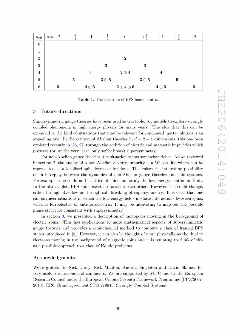
Table 1 summarises the spectrum of framed BPS states for Wilson lines in small

representations of the gauge group.

– 19 –

JHEP06(2014)048

κeff q = −2 −32 −1 −1

2 0 +12 +1 +3

2 +2

0

1

2 2

3 3 3

4 4 2⊕ 4 4

5 5 3⊕ 5 3⊕ 5 5

6 6 4⊕ 6 2⊕ 4⊕ 6 4⊕ 6 6

Table 1. The spectrum of BPS bound states.

5 Future directions

Supersymmetric gauge theories have been used as tractable, toy models to explore strongly

coupled phenomena in high energy physics for many years. The idea that this can be

extended to the kind of situations that may be relevant for condensed matter physics is an

appealing one. In the context of Abelian theories in d = 2 + 1 dimensions, this has been

explored recently in [26, 27] through the addition of electric and magnetic impurities which

preserve (or, at the very least, only softly break) supersymmetry.

For non-Abelian gauge theories, the situation seems somewhat richer. As we reviewed

in section 2, the analog of a non-Abelian electric impurity is a Wilson line which can be

represented as a localised spin degree of freedom. This raises the interesting possibility

of an interplay between the dynamics of non-Abelian gauge theories and spin systems.

For example, one could add a lattice of spins and study the low-energy, continuum limit.

In the ultra-violet, BPS spins exert no force on each other. However this could change,

either through RG flow or through soft breaking of supersymmetry. It is clear that one

can engineer situations in which the low-energy fields mediate interactions between spins,

whether ferroelectric or anti-ferroelectric. It may be interesting to map out the possible

phase structure consistent with supersymmetry.

In section 3, we presented a description of monopoles moving in the background of

electric spins. This has applications to more mathematical aspects of supersymmetric

gauge theories and provides a semi-classical method to compute a class of framed BPS

states introduced in [5]. However, it can also be thought of more physically as the dual to

electrons moving in the background of magnetic spins and it is tempting to think of this

as a possible approach to a class of Kondo problems.

Acknowledgments

We’re grateful to Nick Dorey, Nick Manton, Andrew Singleton and David Skinner for

very useful discussions and comments. We are supported by STFC and by the European

Research Council under the European Union’s Seventh Framework Programme (FP7/2007-

2013), ERC Grant agreement STG 279943, Strongly Coupled Systems

– 20 –

JHEP06(2014)048

Open Access. This article is distributed under the terms of the Creative Commons

Attribution License (CC-BY 4.0), which permits any use, distribution and reproduction in

any medium, provided the original author(s) and source are credited.

References

[1] G. ’t Hooft, Magnetic monopoles in unified gauge theories, Nucl. Phys. B 79 (1974) 276

[INSPIRE].

[2] A.M. Polyakov, Particle spectrum in the Quantum Field Theory, JETP Lett. 20 (1974) 194

[Pisma Zh. Eksp. Teor. Fiz. 20 (1974) 430] [INSPIRE].

[3] N.S. Manton, A remark on the scattering of BPS monopoles, Phys. Lett. B 110 (1982) 54

[INSPIRE].

[4] K.G. Wilson, Confinement of quarks, Phys. Rev. D 10 (1974) 2445 [INSPIRE].

[5] D. Gaiotto, G.W. Moore and A. Neitzke, Framed BPS states, arXiv:1006.0146 [INSPIRE].

[6] O. Aharony, N. Seiberg and Y. Tachikawa, Reading between the lines of four-dimensional

gauge theories, JHEP 08 (2013) 115 [arXiv:1305.0318] [INSPIRE].

[7] A.P. Balachandran, S. Borchardt and A. Stern, Lagrangian and Hamiltonian descriptions of

Yang-Mills particles, Phys. Rev. D 17 (1978) 3247 [INSPIRE].

[8] D. Diakonov and V.Y. Petrov, A formula for the Wilson loop, Phys. Lett. B 224 (1989) 131

[INSPIRE].

[9] C. Beasley, Localization for Wilson loops in Chern-Simons theory, arXiv:0911.2687

[INSPIRE].

[10] M. Stone, Supersymmetry and the quantum mechanics of spin, Nucl. Phys. B 314 (1989) 557

[INSPIRE].

[11] D. Karabali and V.P. Nair, Quantum Hall effect in higher dimensions, Nucl. Phys. B 641

(2002) 533 [hep-th/0203264] [INSPIRE].

[12] S. Elitzur, Y. Frishman, E. Rabinovici and A. Schwimmer, Origins of global anomalies in

quantum mechanics, Nucl. Phys. B 273 (1986) 93 [INSPIRE].

[13] G.V. Dunne, Aspects of Chern-Simons theory, hep-th/9902115 [INSPIRE].

[14] J. Gomis and F. Passerini, Wilson loops as D3-branes, JHEP 01 (2007) 097

[hep-th/0612022] [INSPIRE].

[15] S. Lee and P. Yi, Framed BPS states, moduli dynamics and wall-crossing, JHEP 04 (2011)

098 [arXiv:1102.1729] [INSPIRE].

[16] J.A. Harvey, Magnetic monopoles, duality and supersymmetry, in High energy physics and

cosmology, Trieste Italy (1995), pg. 66 [hep-th/9603086] [INSPIRE].

[17] N.S. Manton and P. Sutcliffe, Topological solitons, Cambridge Univ. Pr., Cambridge U.K.

(2004).

[18] D. Tong, TASI lectures on solitons: instantons, monopoles, vortices and kinks,

hep-th/0509216 [INSPIRE].

[19] E.J. Weinberg, Parameter counting for multi-monopole solutions, Phys. Rev. D 20 (1979)

936 [INSPIRE].

– 21 –

JHEP06(2014)048

[20] M.F. Atiyah and N.J. Hitchin, The geometry and dynamics of magnetic monopoles,

Princeton University Press, Princeton U.S.A. (1988).

[21] G.W. Gibbons and N.S. Manton, The moduli space metric for well separated BPS monopoles,

Phys. Lett. B 356 (1995) 32 [hep-th/9506052] [INSPIRE].

[22] J.M. Maldacena, Wilson loops in large-N field theories, Phys. Rev. Lett. 80 (1998) 4859

[hep-th/9803002] [INSPIRE].

[23] S.-J. Rey and J.-T. Yee, Macroscopic strings as heavy quarks in large-N gauge theory and

anti-de Sitter supergravity, Eur. Phys. J. C 22 (2001) 379 [hep-th/9803001] [INSPIRE].

[24] K. Zarembo, Supersymmetric Wilson loops, Nucl. Phys. B 643 (2002) 157 [hep-th/0205160]

[INSPIRE].

[25] N. Drukker, S. Giombi, R. Ricci and D. Trancanelli, Supersymmetric Wilson loops on S3,

JHEP 05 (2008) 017 [arXiv:0711.3226] [INSPIRE].

[26] A. Hook, S. Kachru and G. Torroba, Supersymmetric defect models and mirror symmetry,

JHEP 11 (2013) 004 [arXiv:1308.4416] [INSPIRE].

[27] A. Hook, S. Kachru, G. Torroba and H. Wang, Emergent Fermi surfaces, fractionalization

and duality in supersymmetric QED, arXiv:1401.1500 [INSPIRE].

[28] D. Tong and K. Wong, Vortices and impurities, JHEP 01 (2014) 090 [arXiv:1309.2644]

[INSPIRE].

[29] Y.-B. Kim and K.-M. Lee, First and second order vortex dynamics, Phys. Rev. D 66 (2002)

045016 [hep-th/0204111] [INSPIRE].

[30] B. Collie and D. Tong, The dynamics of Chern-Simons vortices, Phys. Rev. D 78 (2008)

065013 [arXiv:0805.0602] [INSPIRE].

[31] D. Tong and K. Wong, D-branes, solitons and Wilson lines, to appear.

[32] S.A. Cherkis and B. Durcan, The ’t Hooft-Polyakov monopole in the presence of an ’t Hooft

operator, Phys. Lett. B 671 (2009) 123 [arXiv:0711.2318] [INSPIRE].

[33] H. Murayama, Lecture notes on spin, http://hitoshi.berkeley.edu/221A/spin.pdf.

[34] A. Sen, Dyon-monopole bound states, selfdual harmonic forms on the multi-monopole moduli

space and SL(2, Z) invariance in string theory, Phys. Lett. B 329 (1994) 217

[hep-th/9402032] [INSPIRE].

[35] N. Dorey, D. Tong and S. Vandoren, Instanton effects in three-dimensional supersymmetric

gauge theories with matter, JHEP 04 (1998) 005 [hep-th/9803065] [INSPIRE].

[36] P.H. Cox and A. Yildiz, Bound states with a gauge monopole, Phys. Rev. D 18 (1978) 1211

[INSPIRE].

– 22 –