Hyper-K ahler Geometry, Magnetic Monopoles, and Nahm’s ...jbm18/project-hyperkahler.pdf ·...
78
Hyper-K¨ahler Geometry, Magnetic Monopoles, and Nahm’s Equations John Benjamin McCarthy Jaime Mendizabal Bruno Ricieri Souza Roso Supervised by Professor Michael Singer 3rd May 2019 Project Report Submitted for the London School of Geometry and Number Theory
Transcript of Hyper-K ahler Geometry, Magnetic Monopoles, and Nahm’s ...jbm18/project-hyperkahler.pdf ·...

Hyper-Kahler Geometry, Magnetic Monopoles,and Nahm’s Equations
John Benjamin McCarthyJaime Mendizabal
Bruno Ricieri Souza Roso
Supervised by Professor Michael Singer
3rd May 2019
Project Report Submitted for the London School of Geometry and NumberTheory

Abstract
In this report we investigate the correspondence between SU(2) magneticmonopoles and solutions to the Nahm equations on R3. Further, we invest-igate a variation of this result for singular Dirac monopoles. To this end, thereport starts with a review of the necessary spin geometry and hyper-Kahlergeometry required, as well as the definition of magnetic monopoles and theNahm equations. The final chapter consists of a presentation of Nakajima’sproof of the monopole correspondence, and an investigation of how thesetechniques can be applied to the case of singular Dirac monopoles.
i
Contents
Introduction 1
1 Preliminaries 31.1 Spin Geometry . . . . . . . . . . . . . . . . . . . . . . . . . . . . . 3
1.1.1 Clifford algebras and the Spin group . . . . . . . . . . . . . 31.1.2 Spin and Spinor Bundles . . . . . . . . . . . . . . . . . . . . 61.1.3 Dirac Operators . . . . . . . . . . . . . . . . . . . . . . . . . 8
1.2 Kahler and Hyper-Kahler Manifolds . . . . . . . . . . . . . . . . . . 131.3 Hyper-Kahler Quotients . . . . . . . . . . . . . . . . . . . . . . . . 15
2 Magnetic Monopoles 182.1 Yang-Mills-Higgs Equations . . . . . . . . . . . . . . . . . . . . . . 182.2 SU(2) Monopoles . . . . . . . . . . . . . . . . . . . . . . . . . . . . 192.3 U(1) Monopoles . . . . . . . . . . . . . . . . . . . . . . . . . . . . . 21
2.3.1 Dirac Monopole . . . . . . . . . . . . . . . . . . . . . . . . . 222.3.2 General Case . . . . . . . . . . . . . . . . . . . . . . . . . . 23
2.4 Moduli Space of SU(2) Monopoles . . . . . . . . . . . . . . . . . . . 23
3 Nahm’s Equations 283.1 Instantons . . . . . . . . . . . . . . . . . . . . . . . . . . . . . . . . 283.2 Dimensional Reduction and Nahm’s Equations . . . . . . . . . . . . 29
4 Correspondence between Monopoles and Nahm’s Equations 334.1 SU(2) Monopoles and Nahm’s Equations . . . . . . . . . . . . . . . 33
4.1.1 Monopoles to Solutions of Nahm’s Equations . . . . . . . . . 364.1.2 Solutions of Nahm’s Equations to Monopoles . . . . . . . . . 48
4.2 Singular Monopoles and Nahm’s Equations . . . . . . . . . . . . . . 584.2.1 b-Geometry and the case s = 0 . . . . . . . . . . . . . . . . 604.2.2 sc-Geometry and the case s > 0 . . . . . . . . . . . . . . . . 674.2.3 Limit of Nahm Data . . . . . . . . . . . . . . . . . . . . . . 69
References 73
ii
Introduction
It is a well-known observation in classical electromagnetism that all magnetic fieldsappear to be generated by magnetic dipoles. This is in contrast with electricfields, which may be generated by particles of a single parity. In the landmarkpaper [Dir31] in 1931, Paul Dirac proposed a resolution to the mystery of whyelectric charge is quantized by proposing the existence of magnetic monopoles.Through Dirac’s work, it would be possible to prove that electric charge mustbe quantized provided the existence of even a single magnetic monopole in theuniverse. Despite this and other strong theoretical evidence for the existence ofsuch elementary particles, none have yet been observed.
Mathematically, magnetic monopoles may be modelled as solutions of the Bogo-molny equations on R3,
FA = ?dAΦ.
Similarly to the theory of instantons on R4 modelling other elementary particles,solutions to the Bogomolny equations are gauge-theoretic data on R3, and arehence of considerable mathematical and geometric interest independent of theirphysical origins.
In particular, moduli spaces of solutions to equations such as the Bogomolnyequations are known to, in many cases, provide powerful invariants of the un-derlying spaces, and give new tools for solving many problems in geometry andtopology. This is exemplified by the famous Donaldson theory and Seiberg-Wittentheory in four-manifold topology.
As such, there is much interest in finding new ways of constructing solutions tothese gauge-theoretic equations. The first major breakthrough in this area camewith the novel ADHM construction developed by Atiyah, Drinfeld, Hitchin, andManin in [ADHM78], in order to find solutions of the anti-self-dual Yang-Millsequations on R4 using essentially algebraic data. In [Nah83] Nahm developed, inanalogy with the ADHM construction, a method for constructing solutions to theBogomolny equations from gauge-theoretic data over an interval. In [Hit83] Hitchinshowed that this technique can in fact be used to find all magnetic monopoles,and considerable work was done by many others around this time to extend theseresults to other situations, in particular with varying choices of gauge group.
1
The work of Nahm and Hitchin involved passing through intermediate algebraic-geometric data, spectral curves in twistor spaces. In [Nak93] Nakajima gave apurely differential-geometric proof of the correspondence of Hitchin, phrased inlanguage that is readily generalisable to the theory of Nahm transforms.
In this report, we will review the correspondence between magnetic monopolesand solutions of the Nahm equations through the eyes of Nakajima’s differentialgeometric techniques, and investigate a variation of this result for singular mag-netic monopoles of the simplest type – so called Dirac monopoles.
In Chapter 1 we recall the necessary preliminaries for these constructions, in-cluding elementary spin geometry and the basics of hyper-Kahler geometry.
In Chapter 2 we describe in more detail the definition of a magnetic mono-pole and the construction of the hyper-Kahler moduli space of solutions to theBogomolny equations.
In Chapter 3 the Nahm equations and their relation to the anti-self-dualityequations on R4 are described.
Finally, in Chapter 4 we present (part of) the proof of the correspondence ofmagnetic monopoles with the Nahm equations as shown by Nakajima, as well asan investigation of the correspondence for singular Dirac monopoles. This involvesthe theory of b-geometry and scattering calculus, and a mild amalgamation of theseconcepts applicable in this case.
The authors wish to thank Professor Michael Singer for providing guidancein learning the material presented in this report, and for contributing most of theideas in determining the correspondence between singular magnetic monopoles andappropriate Nahm data.
2

Chapter 1
Preliminaries
In this chapter we will give some preliminary results which will be necessary forthe development of the project.
1.1 Spin Geometry
Here we will lay out the essential definitions and some useful results about Spingeometry and Dirac operators. Many of these concepts can be studied in greatergenerality, but we will often restrict ourselves to the case we are interested in.We will go over many of the results without proofs, specially at the beginning.A more detailed and rigorous exposition can be found Lawson and Michelsohn’sSpin Geometry [LM89], whose notation we follow closely, and in Friedrich’s DiracOperators in Riemannian Geometry [Fri00].
1.1.1 Clifford algebras and the Spin group
Definition 1.1.1. Let (V, q) be a vector space with a quadratic form. Its Cliffordalgebra is defined as
Cl(V, q) := T (V )/Iq(V ),
where
T (V ) =∞⊕k=0
V ⊗k
is the tensor algebra of V and Iq(V ) is the ideal of T (V ) generated by elementsof the form v ⊗ v + q(v) for v ∈ V .
The product of two elements ϕ, ψ ∈ Cl(V, q) will be denoted by ϕ ·ψ, or simplyby ϕψ.
3
In other words, the Clifford algebra of a vector space is the algebra generatedby V under the relations v2 = −q(v)1 for v ∈ V . Equivalently, if q(v, w) =12(q(v+w)−q(v)−q(w)) is the polarisation of the quadratic form (if the underlying
field has characteristic different from 2), then we have the relations
v · w + w · v = −2q(v, w).
It can be shown that Cl(V, q) is isomorphic to∧•V as a vector space (it will be
isomorphic as an algebra precisely when q ≡ 0). In particular, V will be naturallyembedded as a vector space.
From now on, for simplicity, we will take our vector space to be finite dimen-sional and real, and we will take the quadratic form to be positive definite. Thismeans that (V, q) will be isomorphic to Rn with the standard metric, for some n.Whenever we take (V, q) to be explicitly Rn with the standard metric, we will writeCl(n) for the Clifford algebra. It will be useful to consider as well the complexi-fication of the Clifford algebra, which will be denoted by Cl(V, q) := Cl(V, q)⊗C.
Firstly, let us consider
Cl×(V, q) = ϕ ∈ Cl(V, q) : ∃ϕ−1 such that ϕϕ−1 = ϕ−1ϕ = 1,
which has a group structure. This group is, in fact, a Lie group of dimension 2n,and its Lie algebra can be identified with Cl(V, q), with the Lie bracket being thecommutator [x, y] = xy− yx. Furthermore, analogously to matrix Lie groups, theadjoint representation on the Lie algebra is given by conjugation.
We can now define the Spin group as a subgroup of Cl×(V, q).
Definition 1.1.2. Given (V, q), we define the Spin group as
Spin(V, q) := v1v2 · · · v2k ∈ Cl(V, q) : vi ∈ V and q(vi) = 1.
That is, it is the subgroup of Cl×(V, q) formed by products of an even amount ofunit vectors. It forms a group, since multiplying two elements clearly gives anotherelement of the group, and the element v2k · · · v2v1 is the inverse of v1v2 · · · v2k.Again, if (V, q) is taken to be explicitly Rn with the standard metric, then wedenote the Spin group by Spin(n).
The Spin group acts on Cl(V, q) through the adjoint representation, and canbe shown that this action actually preserves V ⊂ Cl(V, q). This gives a grouphomomorphism ξ : Spin(V, q) → SO(V, q). It turns out that this is actually acovering.
Theorem 1.1.3. Given (V, q), the map ξ : Spin(V, q)→ SO(V, q) is a 2-to-1 cov-ering. Furthermore, if the dimension of V is greater than 1, then this covering isnot trivial, and if it is greater than 2, this is the universal cover. In particular, theLie algebras of both groups are isomorphic (and from now on will be identified).
4
Note that, if we have a representation of SO(V, q), we can pull it back to arepresentation of Spin(V, q). However, if we have a representation of Cl(V, q), thenwe can restrict it to a representation of Spin(V, q) which will not factor throughSO(V, q).
There are, in particular, some preferred representations.Let us first see what the Clifford algebras look like. It turns out that both
Cl(n) and Cl(n) can be easily identified with matrix algebras over R, C or H. Weare particularly interested in the complexified Clifford algebras.
Proposition 1.1.4. The complexified Clifford algebras can be written as
Cl(n) = C(2k) if n = 2k,
Cl(n) = C(2k)⊕ C(2k) if n = 2k + 1,
where C(2k) is the algebra of 2k × 2k matrices over the complex numbers.
In view of this result, we can see that there are some obvious representations:for n = 2k, the representation on C2k , and for n = 2k+1 the two representations onC2k given by acting with each of the two components. It turns out that these are,in fact, the only irreducible (real or complex) representations up to isomorphism.Since Clifford algebra representations split as sums of irreducible representations,these are going to be the most important representations.
Now, if we restrict our representation to Spin(n) ⊂ Cl(n), we obtain repres-entations of the Spin group. In the even case, the representation splits into twoinequivalent irreducible representations, and in the odd case, the resulting rep-resentation is irreducible and independent of the choice of representations of theClifford algebra. We denote these representations by ∆C
2k = ∆C+2k ⊕∆C−
2k and ∆C2k+1.
We can establish some further properties of these representations. In particular,we would be interested in knowing how vectors in the original n-dimensional vectorspace act in these representations.
In the case n = 2k, the space of the representation is C2k . As mentioned before,it can be split as C2k = C2k−1 ⊕ C2k−1
. We can then find a basis of R2k such that
the first 2k − 1 vectors act as
(0 σiσi 0
), where the σi are the actions of a basis
of Rk−1 on the space C2k−1given by the irreducible Clifford action of the case
2k − 1, and where the last vector acts like
(0 −11 0
). In particular, the action of
the elements of R2k interchanges the spaces of the representations ∆C+2k and ∆C−
2k .
In the case n = 2k+1, the space of the representation is C2k , like in the case ofdimension 2k. Then, we can choose a basis of R2k+1 such that the first 2k vectorsact as a basis of R2k act in the corresponding representation, and where the last
vector acts as
(i 00 −i
), following the splitting of the previous case.
5
1.1.2 Spin and Spinor Bundles
In a similar way to how we developed a theory of Clifford algebras and Spin groupsover a vector space with a metric, we can try to develop it for a Riemannian vectorbundle E over a manifold M (for example, the tangent bundle of a Riemannianmanifold).
If we have such a vector bundle we have can construct its Clifford bundleanalogously of how we did before.
Definition 1.1.5. Given a vector bundle E with a metric g over a manifold M ,we define the Clifford bundle of E as
Cl(E) = T (E)/Ig(E),
where T (E) is the tensor bundle of E and Ig(E) is the bundle of ideals whichgenerated at each fibre by elements of the form v ⊗ v + g(v).
Note that this bundle is isomorphic, as a vector bundle, to∧•(E).
We can describe this bundle in an alternative way using the theory of associ-ated bundles. Suppose that E is orientable, and let P be its associated principalSO(n)-bundle. Then, since any orthogonal automorphism of Rn extends to anautomorphism of Cl(n), we can form the associated bundle through the action ofSO(n) on Cl(n). This will be precisely Cl(E).
Now we want to construct the analogous to the Spin group, which should bea principal Spin(n)-bundle. Note, however, that simply restricting the Cliffordbundle to its Spin group will not always give a principal Spin(n) structure, sincethe Clifford bundle is not itself a principal bundle.
The proper notion of the Spin bundle of E will be, rather, a lifting of the SO(n)structure.
Definition 1.1.6. Let E be an orientable Riemannian vector bundle, and let Pbe its associated principal SO(n)-bundle. We say Q is a spin structure of E if itis a principal Spin(n)-bundle and has a 2-to-1 covering of P which is equivariantthrough the covering of SO(n) by Spin(n).
Such a structure does not always exist, and when it does, it is not necessarilyunique. We have the following characterisation.
Theorem 1.1.7. An orientable Riemannian vector bundle E has a Spin structureif and only if its second Stiefel-Whitney class is zero. Furthermore, in this case,the possible Spin structures are in one to one correspondence with elements ofH1(M ;Z2).
6

Hence, for example, there exists a unique spin structure on the 2-sphere or onR3 with any finite amount of points removed (these spaces will come up in laterchapters).
These spin structures can be used to construct bundles.
Definition 1.1.8. Let ρ : Cl(n) → End(W ) be a representation of a Cliffordalgebra on a vector spaceW . If we have a Spin(n) structureQ→M , the associatedreal spinor bundle is defined as S(E) = Q ×ρ W over M , where ρ is taken to bethe restriction to Spin(n) ⊂ Cl(n).
If ρ : Cl(n) → End(W ) is a complex representation of the complex Cliffordalgebra, then the associated bundle is a complex spinor bundle.
For example, one may construct a complex spinor bundle using an irreduciblerepresentation of the Clifford algebra, as described above. This means that thespinor bundle will be associated through the representation ∆C
n . If n is even, sincethis representation splits, it will give a splitting of the vector bundle into the directsum of two bundles, sometimes called the positive and negative spinor bundles.
One of the main features of these spinor bundles is that the representation ofthe Clifford algebra on the vector space gives a fibre-wise representation of theClifford bundle on the spinor bundle. This fact is easy to see by defining theClifford bundle as an associated bundle of the Spin bundle (through the adjointaction).
Proposition 1.1.9. In the conditions above, there exists an action of each fibreof the Clifford bundle Cl(E) on each fibre of the spinor bundle S(E). This alsoholds for complex spinor bundles.
In particular, each element of the original bundle E gives an automorphism ofthe corresponding fibre of S(E), which we call Clifford multiplication.
Furthermore, if our original bundle E had a connection (compatible with themetric), we can use it to construct a connection on the spinor bundle.
In order to do this, consider the connection 1-form ω ∈ Ω(P ; so(n)). Since Qcovers P , we can pull back the 1-form to get a 1-form of the principal Spin(n)-bundle Q, with values in spin(n) ∼= so(n), which will satisfy the appropriate condi-tions to define a connection on Q. Since S(E) is an associated bundle to Q, we geta connection on S(E). In our case, we will assume that the elements of Spin(n)(and indeed any unit vector of Cl(n)) act by isometries on W (this can always beachieved by an appropriate choice of metric on W ).
We also assume that ρ is faithful, we can embed Q in the principal SO(m)-bundle of of the spinor bundle, using the homomorphism Spin(n)→ SO(m) (choos-ing a basis for W ).
Note that this provides another way to construct the spin connection: this givesa map spin(n)→ so(m), which allows us to extend the 1-form to a so(W )-valued
7

1-form on the principal SO(m)-bundle of S(E), which will, once again, satisfy theappropriate conditions to be a connection 1-form.
This connection (which will be compatible with the metric of S(E)) can beexpressed locally in terms of the connection 1-form of the original connection. Inorder to do that, first pick a local orthonormal frame e1, . . . , en of E. This gives alocal section of P , which lifts (in two different ways) to a section of Q. Throughthe embedding of Q in the principal SO(m)-bundle of S(E), we obtain a sectionof the latter, which provides an orthonormal frame σ1, . . . , σm of S(E) (note thatthis frame will depend on the choice of lifting only by a sign).
Now, let ω = ω ji be the local connection 1-form (so that ∇Eei = ω j
i ej). Withrespect to the local frame σ1, . . . , σm, the connection 1-form will be
ωS =1
4
n∑i,j=1
ω ji eiej, (Eq. 1.1)
where eiej represents Clifford multiplication by the corresponding vectors.
1.1.3 Dirac Operators
One of the main motivations for spin geometry and spinor bundles is that we candefine on them a certain kind of operators which have very interesting properties.
Definition 1.1.10. Let S be a bundle over a Riemannian manifold M with a(fibrewise) action of the Clifford bundle Cl(TM). Suppose that S has a metricsuch that the action by unit tangent vectors is an isometry, and suppose that ithas a connection ∇S compatible with the metric. The Dirac operator on S is theoperator D : Γ(S)→ Γ(S) defined locally by
D(s) =n∑i=1
ei · ∇Seis,
where e1, . . . , en is a local orthonormal frame of vector fields and s ∈ Γ(S).
An important case is that in which the bundle is the spinor bundle constructedfrom a spin structure of the tangent bundle through the irreducible action describedabove, and the connection on it is the connection induced by the Levi-Civitaconnection on the tangent bundle. From now on, we will use /S to refer to thisbundle (or /SM if the manifold M needs to be specified) and we will use /D to referto its Dirac operator. Therefore, /S is a complex vector bundle of (complex) rank2n, where n is the (real) dimension of the manifold. Furthermore, if n is even,we will be able to write it in terms of the positive and negative spinor bundles/S = /S
+⊕ /S−. In this case, /D can be split into two operators, /D+
: Γ(/S+
)→ Γ(/S−
)
8
and /D−
: Γ(/S−
) → Γ(/S+
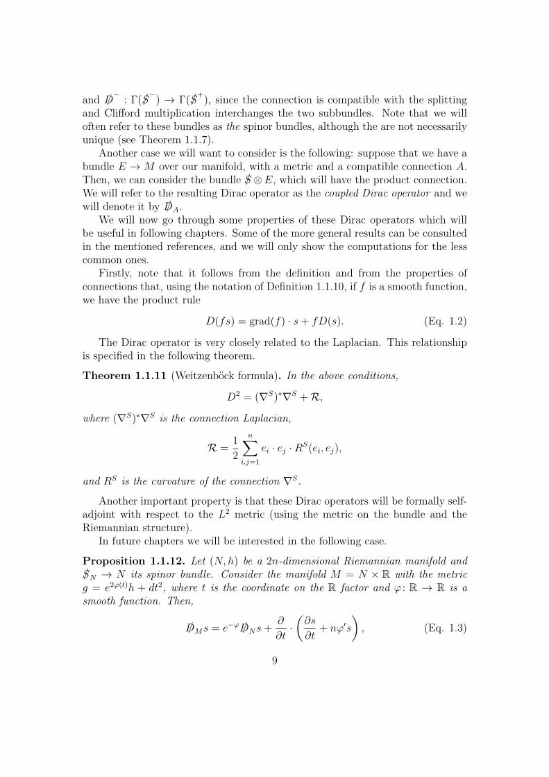
), since the connection is compatible with the splittingand Clifford multiplication interchanges the two subbundles. Note that we willoften refer to these bundles as the spinor bundles, although the are not necessarilyunique (see Theorem 1.1.7).
Another case we will want to consider is the following: suppose that we have abundle E →M over our manifold, with a metric and a compatible connection A.Then, we can consider the bundle /S ⊗E, which will have the product connection.We will refer to the resulting Dirac operator as the coupled Dirac operator and wewill denote it by /DA.
We will now go through some properties of these Dirac operators which willbe useful in following chapters. Some of the more general results can be consultedin the mentioned references, and we will only show the computations for the lesscommon ones.
Firstly, note that it follows from the definition and from the properties ofconnections that, using the notation of Definition 1.1.10, if f is a smooth function,we have the product rule
D(fs) = grad(f) · s+ fD(s). (Eq. 1.2)
The Dirac operator is very closely related to the Laplacian. This relationshipis specified in the following theorem.
Theorem 1.1.11 (Weitzenbock formula). In the above conditions,
D2 = (∇S)∗∇S +R,
where (∇S)∗∇S is the connection Laplacian,
R =1
2
n∑i,j=1
ei · ej ·RS(ei, ej),
and RS is the curvature of the connection ∇S.
Another important property is that these Dirac operators will be formally self-adjoint with respect to the L2 metric (using the metric on the bundle and theRiemannian structure).
In future chapters we will be interested in the following case.
Proposition 1.1.12. Let (N, h) be a 2n-dimensional Riemannian manifold and/SN → N its spinor bundle. Consider the manifold M = N × R with the metricg = e2ϕ(t)h + dt2, where t is the coordinate on the R factor and ϕ : R → R is asmooth function. Then,
/DMs = e−ϕ /DNs+∂
∂t·(∂s
∂t+ nϕ′s
), (Eq. 1.3)
9

for s ∈ Γ(/SM), where /SM is identified with the pullback of /SN through the projec-tion in order to apply /DN , and where ∂
∂t· indicates Clifford multiplication by the
vector field in the direction of the coordinate t.
Proof. The identification between the pullback of /SN and /SM can be seen throughthe construction of the spinor bundles, since we can construct the spin bundle ofM by taking the pullback of a spin bundle on N and taking the associated bundleusing the action of Spin(2n) on Spin(2n+ 1) given by left multiplication (since itis a subgroup). This will give a spin bundle on M , and the corresponding spinorbundle will be isomorphic (as a vector bundle) to the pullback of /SN , since theirreducible representations of Cl(2n) and Cl(2n+ 1) are on the same vector space.Furthermore, vectors orthogonal to ∂
∂twill act in the same way.
Now, let f1, . . . , f2n be local orthonormal vector fields on N . Then, the Levi-Civita connection with respect to h will be give by local 1-forms θ ji , with 1 ≤i, j ≤ 2n, such that ∇Nfi = θ ji fj. We denote θ j
ki = θ ji (fk).The vector fields f1, . . . , f2n can also be though at vector fields on M in the
direction of N , and by setting ei = e−ϕfi, for 1 ≤ i ≤ 2n and letting e0 be thevector field in the direction of t, we get a local basis of orthonormal vectors on M .Then, the Levi-Civita connection with respect to g will have the form∇Mei = ω j
i ejfor some local 1-forms ω j
i , with 0 ≤ i, j ≤ 2n. Analogously to before, we writeω jki = ω j
i (ek).Some elementary and not too enlightening computations will tell us that
ω jki =
e−ϕθ j
ki if i, j, k 6= 0ϕ′δkj if i = 0 and j, k 6= 0−ϕ′δki if j = 0 and i, k 6= 00 otherwise.
Note, in particular, that ω j0i = ω 0
k0 = 0.We note, also, that Clifford multiplication in by fi in /SN is the same as Clifford
multiplication by ei in /SM (under the identification).If σ1, . . . , σm is the local orthonormal basis of /SM (and /SN) corresponding to
e1, . . . , e2n (and f1, . . . , f2n), we can compute the Dirac operator using (Eq. 1.1).
10
We have
/DM(σ`) =2n∑k=0
ek · ∇/SMekσ`
=2n∑k=0
ek · ωS(ek)σ`
=1
4
2n∑k=0
ek ·
(2n∑i,j=0
ω jki ei · ej · σ`
)
=1
4
2n∑k=1
ek ·
(2n∑i,j=1
ω jki ei · ej · σ`
)
+1
4
2n∑k=1
ek ·
(2n∑j=1
ω jk0 e0 · ej · σ`
)+
1
4
2n∑k=1
ek ·
(2n∑i=1
ω 0ki ei · e0 · σ`
)
=1
4e−ϕ
2n∑k=1
fk ·
(2n∑i,j=1
θ jki fi · fj · σ`
)
+1
4ϕ′
(2n∑k=1
ek · e0 · ek · σ` −2n∑k=1
ek · ek · e0 · σ`
)=e−ϕ /DN(σ`) + nϕ′σ`,
which is exactly (Eq. 1.3) for elements in the basis. Therefore, it only remains tocheck that the operator /DM defined in (Eq. 1.3) satisfies the appropriate productrule (Eq. 1.2). For that, let s ∈ Γ(/SM) and f ∈ C∞(R). Then,
/DM(fs) =e−ϕ /DN(fs) +∂
∂t·(∂fs
∂t+ nϕ′fs
)=e−ϕ grad(N,h)(f) · s+ e−ϕf /DN(s) +
∂f
∂te0 · s+ fe0 · s+ nϕ′fs
=
(e−ϕ grad(N,h)(f) +
∂f
∂te0
)· s+ f( /DN(s) + nϕ′s)
= gradg(f) · s+ f /DM(s),
as we wanted (note that, when using the product rule for /DN , we would get Cliffordmultiplication of the gradient of f with respect to h (which is tangent to the Ncomponent and might depend on t), but through the identification with /SM , thisis the same as Clifford multiplication by part of the gradient with respect to gwhich is tangent to the N component multiplied by e−ϕ).
11
We can write this in a slightly nicer way by considering the relationship betweenthe Clifford algebra representations for 2n and 2n+ 1.
Corollary 1.1.13. In the conditions above, we have
/DM =
(i(∂∂t
+ nϕ′)
e−ϕ /D−N
e−ϕ /D+N −i
(∂∂t
+ nϕ′)) .
Proof. This follows from Proposition 1.1.12 and the discussion above about theirreducible representations of Clifford algebras.
We conclude this section by recalling the special case of the spin Dirac operatoron a spin Kahler manifold. See [Fri00, §3.4] for more details. It was observed byHitchin in [Hit74] that a Kahler manifold is spin if and only if the canonical bundleadmits a square root (and in fact there is a one-to-one correspondence between spinstructures and holomorphic square roots). In this setting we have the followingtheorem.
Theorem 1.1.14. Let M be a Kahler manifold of dimension dimCM = n ad-mitting a holomorphic square root of KM , and let L → M any such holomorphicsquare root. Then with respect to the corresponding spin structure, there is anisomorphism
/S ∼= (∧
0,0 ⊕∧
0,1 ⊕ · · · ⊕∧
0,n)⊗ L,
with the splitting /S = /S+ ⊕ /S
−corresponding to
/S+ ∼=
∧0,even ⊗ L, /S
− ∼=∧
0,odd ⊗ L.
Furthermore the spin Dirac operator on /S is
/D =√
2(∂ + ∂∗).
Notice that the factor of√
2 agrees with the Kahler identity that ∂2
= 2∆∂ =∆d.
This result may be extended to the case of coupled Dirac operators. In particu-lar, if E is a Hermitian holomorphic vector bundle over M with Chern connection∇ and S := /S ⊗ E is a Dirac bundle with coupled spin connection ∇S, thenTheorem 1.1.14 becomes the following.
Theorem 1.1.15. If D is the coupled Dirac operator on S = /S⊗E defined by thecoupled spin connection ∇S coming from the Chern connection on E → M , thenwith respect to the splitting
S ∼= (∧
0,0 ⊕∧
0,1 ⊕ · · · ⊕∧
0,n)⊗ L⊗ E∼= (∧
0,0(E)⊕∧
0,1(E)⊕ · · · ⊕∧
0,n(E))⊗ L,
12

we have the corresponding splitting S = S+ ⊕ S− with
S+ ∼=∧
0,even(E)⊗ L, S− ∼=∧
0,odd(E)⊗ L,
andD =
√2(∂EL + ∂
∗EL)
where ∂EL = ∇0,1 is the Dolbeault operator on E ⊗ L.
1.2 Kahler and Hyper-Kahler Manifolds
Recall the definition of a Kahler manifold.
Definition 1.2.1. A Kahler manifold is a triple (M, g, I) where (M, g) is a Rieman-nian manifold, and I is an integrable almost-complex structure on M such that Iis orthogonal with respect to g, and if one defines
ω(X, Y ) = g(IX, Y )
then the 2-form ω is closed.
The condition that dω = 0 above is called the Kahler condition. Kahler man-ifolds are Riemannian complex manifolds such that the two structures are com-patible in the right sense. Namely, there is a list of equivalent conditions to theKahler condition, which justify this statement.
Proposition 1.2.2. Let M be a complex manifold with Riemannian metric g,associated integrable almost-complex structure I, and Levi-Civita connection ∇.Then the following are equivalent:
1. h = g + iω is a Kahler metric,
2. dω = 0,
3. ∇I = 0,
4. the Chern connection of the Hermitian metric h := g + iω on TM agreeswith the Levi-Civita connection ∇,
5. in terms of local holomorphic coordinates, we have
∂gjk∂z`
=∂g`k∂zj
,
6. for each point p ∈ M there is a smooth real function F in a neighbourhoodof p such that ω = i∂∂F , and F is called the Kahler potential, and
13

7. for each point p ∈ M there are holomorphic coordinates centred at p suchthat g(z) = 1 +O(|z|2).
Kahler manifolds have many nice properties that general complex manifolds donot have, such as a Hodge decomposition of their complex de Rham cohomologyinto Dolbeault components. See [WGP80], [GH78], or [Bal06] for more details.
Notice that by the above proposition, for a Kahler manifold (M, g, I) we have
∇I = 0, ∇g = 0
where∇ is the Levi-Civita connection. Combining these two identities tells us thatthe holonomy of the Levi-Civita connection on a Kahler manifold will preserve boththe complex and Riemannian structures. Indeed we have
Hol(g) ⊆ GL(n,C) ∩O(2n) = U(n)
where n is the complex dimension of M . The converse is also true.
Theorem 1.2.3. A manifold (M, g) is Kahler if and only if Hol(g) ⊆ U(n).
Kahler manifolds appear as one part of Berger’s classification of Riemannianholonomy groups. The classification includes several other subgroups of GL(2n,R).For example, if we have Hol(g) ⊆ SU(n) = U(n) ∩ SL(n,C) then M is Calabi-Yau (in fact one usually requires compactness in the definition of Calabi-Yaumanifolds). If further we have
Hol(g) ⊆ Sp(m) = SU(n) ∩ Sp(n,C),
where n = 2m, then M is hyper-Kahler. The above expression for Sp(m) corres-ponds to the Levi-Civita connection preserving a holomorphic symplectic form onM , but using the equality
Sp(m) = SU(n) ∩ Sp(n,C) = O(2n) ∩GL(m,H)
we see that a hyper-Kahler structure implies that the Levi-Civita connection pre-serves a representation of the quaternions on the tangent bundle of M .
This gives an alternative characterisation of hyper-Kahler manifolds, which wetake as the definition.
Definition 1.2.4 (Hyper-Kahler Manifold). A hyper-Kahler manifold is a quin-tuple (M, g, I, J,K) where (M, g) is a Riemannian manifold, and I, J, and K arethree integrable almost-complex structures on M , each orthogonal for g, such that
I2 = J2 = K2 = IJK = −1.
14
Notice that the above definitions require that the dimension of M be a multipleof four. The first example of a hyper-Kahler manifold is therefore H itself. Indeedunder the identification H = C2 = R4 we have the standard Riemannian metric
g = dx21 + dy2
1 + dx22 + dy2
2
with three compatible almost-complex structures coming from writing a vector asx1 + iy1 + jx2 + ky2, and multiplying by i, j, and k respectively. From the hyper-Kahler structure on H we can obtain a larger class of flat hyper-Kahler manifoldssimply by taking the tensor product with a fixed vector space.
In particular, let G be a Lie group admitting a bi-invariant metric on its Liealgebra g, say B. Let M = g ⊗ H. Then M admits a hyper-Kahler structure bycombining the three Kahler forms on H with the bi-invariant metric on g. Such aflat example of a hyper-Kahler manifold comes with an action of G by the adjointaction in the first factor, and bi-invariance implies that this action preserves thehyper-Kahler structure. We will see in the next section how this allows one toconstruct many examples of interesting hyper-Kahler manifolds as quotients offlat hyper-Kahler manifolds.
1.3 Hyper-Kahler Quotients
At the end of the previous section we saw examples of flat hyper-Kahler manifolds.One way to obtain more interesting examples is by taking quotients. Given a sym-plectic manifold (M,ω), there is a well-developed theory of symplectic reduction.Namely, if a group G acts on (M,ω) preserving the symplectic form in such a waythat a moment map µ : M → g∗ exists, where µ is equivariant (using the co-adjointaction on g∗) and satisfies
d〈µ,X〉 = −ιX#ω,
for every X ∈ g, thenMred := µ−1(0)/G
inherits a symplectic structure, with a form ωred satisfying π∗ωred = ι∗ω forι : µ−1(0) → M and π : µ−1(0) → Mred. This is the Marsden-Weinstein quotientof M by G.
When M has a compatible complex structure, that is, when M is Kahler, andwhenG acts holomorphically, the quotientMred will also inherit a Kahler structure.There are many interesting examples of Kahler manifolds constructed in this way.For example the action of S1 on Cn+1 admits a moment map µ(z) = 1
2|z|2− 1
2, and
the Kahler reduction µ−1(0)/S1 = S2n+1/S1 is CPn with the Fubini-Study Kahlerform.
15

When M is hyper-Kahler, under suitable assumptions we can extend this the-ory. Namely, suppose a group G acts on M preserving the hyper-Kahler structure,in the sense that G acts holomorphically with respect to I, J , and K, and admitsa moment map with respect to each of the three Kahler forms ωI , ωJ , and ωK .Then one can build a hyper-Kahler moment map µ : M → g∗ ⊗ R3 defined by
µ = (µI , µJ , µK).
Assuming 0 is a regular value and G acts freely on µ−1(0), there is a hyper-Kahlerreduction
M///G := µ−1(0)/G
of M by G, with hyper-Kahler structure inherited as in the case of regular sym-plectic reduction. In particular we have an inclusion ι : µ−1(0) → M and a pro-jection π : µ−1(0) → M///G, and again ι∗ωI = π∗ωI,red and similarly for J andK.
Most interesting examples of hyper-Kahler manifolds are obtained by somekind of hyper-Kahler reduction, often-times infinite-dimensional. We will see twofundamental examples (and two of the first examples) of this infinite-dimensionalreduction in Chapters 2 and 3, but first we will study a more fundamental finite-dimensional example.
Recall that M = g ⊗ H admits a flat hyper-Kahler structure when g is theLie algebra of a compact real Lie group, and so admits a bi-invariant metric. Thespace M is acted upon by G through the adjoint action preserving the quaternionicstructure, and so this action admits a moment map as follows.
Let X ∈ g. Then the fundamental vector field X# is defined by
X#∣∣Y
:=d
dt(ad(exp(tX))Y )t=0
where Y = Y0 + iY1 + jY2 + kY3 ∈ g⊗H. This is just the derivative of ad, whichis well-known to be given by the Lie bracket itself. Namely
X#∣∣Y
= [X, Y0] + i[X, Y1] + j[X, Y2] + k[X, Y3].
If B denotes the bi-invariant metric on g, then the form ωI is given by
ωI(Z,W ) = 〈iZ,W 〉 = −B(Z1,W0) +B(Z0,W1)−B(Z3,W2) +B(Z2,W3)
and so if Z ∈ TY (g⊗H) ∼= g⊗H then
ιX#ωI |Y (Z) = −B([X, Y1], Z0) +B([X, Y0], Z1)−B([X, Y3], Z2) +B([X, Y2], Z3).
16

Theorem 1.3.1. The action of G on g⊗H has a moment map µ = (µI , µJ , µK)given by
µI(T0, T1, T2, T3) = [T0, T1] + [T2, T3],
µJ(T0, T1, T2, T3) = [T0, T2] + [T3, T1],
µK(T0, T1, T2, T3) = [T0, T3] + [T1, T2].
Proof. We will just check µI , the other cases being completely analogous. Observewe have
µI(Y + sZ) = [Y0 + sZ0, Y1 + sZ1] + [Y2 + sZ2, Y3 + sZ3],
d
ds
∣∣∣∣s=0
µI(Y + sZ) = [Y0, Z1] + [Z0, Y1] + [Z2, Y3] + [Y2, Z3].
Taking an inner product with X and using bi-invariance of B, we obtain preciselyιX#ωI |Y (Z) as computed above, showing that
d〈µI , X〉 = ιX#ωI
for all X ∈ g, as desired.
Most examples of hyper-Kahler constructions known are some variation of thesemoment map equations, such as coadjoint orbits, Higgs moduli spaces, monopolemoduli spaces, and Nahm’s equations. For an exposition of such examples, see thearticle [Hit92] of Hitchin. We will point out the most immediate and importantexample of this phenomenon now, and mention some others in passing later.
Remark 1.3.2. If we replace Ti by ∇i where ∇ is a connection arising from aprincipal G-bundle over R4 then the resulting moment map equations are
F01 = F32,
F02 = F13,
F03 = F21,
which are just the anti-self dual Yang-Mills equations viewed as a single equationµ = 0. See Section 3.1 for more discussion of this example.
17
Chapter 2
Magnetic Monopoles
2.1 Yang-Mills-Higgs Equations
Let M be a 3-dimensional Riemannian manifold, G a semisimple compact Liegroup, P → M a principal G-bundle, and let A ⊂ Ω1(P ; g) denote the space ofconnections on P .
Definition 2.1.1. The Yang-Mills-Higgs functional is
YMH : A× Γ(ad(P ))→ R, YMH(A,Φ) :=
∫M
|FA|2 + |dAΦ|2,
where the inner product on g is given by minus the Killing form.
Proposition 2.1.2. The Euler-Lagrange equations for YMH read:
dA ? FA = −[Φ, dAΦ],
dA ? dAΦ = 0
When (A,Φ) solves the equations above, Φ is referred to as the Higgs field.
Remark 2.1.3. Note that, if M be compact, there cannot be non trivial solutions,since, integrating by parts,∫
M
|dAΦ|2 =
∫M
(dA ? dAΦ,Φ) = 0.
Thus the Higgs field is covariantly constant and the connection must simply satisfythe usual Yang-Mills equations. Hence, one should consider M non compact.
Henceforth, we shall work with M = R3 and M = R3 \ P , where P is somefinite set of points.
18
We shall focus on solutions subject to the further conditions:
YMH(A,Φ) <∞, |Φ(x)| → 1 as r := |x| → ∞ (Eq. 2.1)
The second of these is referred to as the Prasad-Sommerfield limit. It is shown in[JT80] that these conditions imply
|FA| = O(r−2),
|dAΦ| = O(r−2),∣∣∣∣∂Φ
∂Ω
∣∣∣∣ = O(r−2), and
|Φ(x)| = 1 +m
r+O(r−2),
where m ∈ R is some constant.
2.2 SU(2) Monopoles
Firstly, we shall look at the simplest example of M = R3 and G = SU(2).To start off, we make some remarks about the asymptotic behaviour of the
Higgs field. Given a solution (A,Φ) to the Yang-Mills-Higgs equations satisfyingthe conditions above, fix some small ε > 0 and let R > 0 be large enough sothat, for any |x| ≥ R, |Φ(x)| has two distinct eigenvalues, say λ1, λ2 which satisfy|i − λ1| < ε and |i + λ2| < ε. The values of λ1, λ2 may of course depend on x,but the point is that one may speak of the eigenvalue near ±i. The reason thisis possible is because any element of su(2) with unit length squares to −1, so itseigenvalues are ±i, and it is also tracefree, so that it have distinct eigenvalues.
Granted this, define a line bundle LΦ → SR, where the fibre over x consists ofthe eigenspace of Φ(x) with eigenvalue near i. Note that, even though the bundleP → R3 is trivial, the line bundle LΦ need not be trivial. Let k ∈ Z ∼= H2(SR)denote the degree of LΦ. It can be shown that k is independent of R.
Definition 2.2.1. The integer k is called magnetic charge of the solution (A,Φ).
Remark 2.2.2. The charge k can be computed simply as the degree of the map|Φ|−1Φ : SR → S2, where R > 0 is large and S2 ⊂ su(2) is the unit sphere.
For large R, let BR be the ball of radius R and consider:∫BR
|FA|2 + |dAΦ|2 =
∫BR
|FA − ?dAΦ|2 + 2(?dAΦ, FA)
19
Where (·, ·) denotes the combination of the inner product on su(2) with the innerproduct of forms. Now:
d(Φ, FA) = (dAΦ, FA)− (Φ, dAFA) = (dAΦ, FA) = ?(?dAΦ, FA)
Hence, by Stokes: ∫BR
(?dAΦ, FA) =
∫SR
(Φ, FA)
Meanwhile, one can use Chern-Weil theory to show that:
limR→∞
∫SR
(Φ, FA) = 4πk
Hence, if we add the assumption that k ≥ 0:
YMH(A,Φ) =
∫R3
|FA − ?dAΦ|2 + 8πk ≥ 8πk
Thus, the functional is minimized whenever FA = ?dAΦ.
Definition 2.2.3. Let M be a 3-manifold, P → M be a principal G-bundle, Aa connection on P and Φ ∈ Γ(adP ). The equation FA = ?dAΦ is called theBogomolny equation.
Definition 2.2.4. In the case M = R3 and G = SU(2), a solution of the Bogo-molny equation subject to k ≥ 0, where k is the magnetic charge, and the Prasad-Sommerfield boundary conditions above is referred to as an SU(2) magnetic mono-pole of charge k.
Remark 2.2.5. The constant m in the asymptotic behaviour of Φ turns out toonly depend on the charge k. Indeed, m = −k
2.
Example 2.2.6. It is possible to write down explicit solutions which have a rel-atively simple form. For example, the pair (A,Φ) with
A =∑i,j,`
(|x|
sinh |x|− 1
)εij`
x`|x|
ei√2⊗ dxj
Φ =∑i
(|x| coth |x| − 1)xi|x|2
ei√2
is a monopole of charge 1, where ei denote the Pauli matrices. Note it has anSO(3) symmetry. This solution is called the Prasad-Sommerfield monopole; see[TM79] for a derivation. It can be shown that this is the only monopole of charge1 up to translation and gauge equivalence.
20

Remark 2.2.7. It is worth noting that a solution (A,Φ) to the Bogomolny equa-tion defines via:
Φdx0 + A1dx1 + A2dx2 + A3dx3
an ASD connection on the trivial SU(2)-bundle over R4; conversely, any ASDconnection on the trivial bundle which be constant on some direction defines amonopole. This “dimensional reduction” is another way to think of monopoles andit is how Taubes proves the necessary analytical results in [Tau83]. See Section 3.2for more discussion of this phenomenon.
2.3 U(1) Monopoles
Consider, now, the case of G = U(1). Notice that, if M = R3, then, since U(1) isabelian, the Yang-Mills-Higgs equations imply dA ? dAΦ = d ? dΦ = 0. Togetherwith the Prasad-Sommerfield limit, this means that Φ is a bounded harmonicfunction, and hence it is constant. Therefore, solutions on R3 are uninteresting,and consequently we turn our attention to M = R3 \ P , for P ⊂ R3 a finite set ofpoints. Notice that, in this case, the bundle P →M need not be trivial.
There is a notion of magnetic charge here as well, and the definition is analog-ous: select some large ball BR ⊂ R3 so as to have P ⊂ BR. Consider the restrictionP |M\BR
, and define the magnetic charge k ∈ Z ∼= H2(R3 \BR) to be the degree ofthis line bundle. The Bogomolny equation has the same relevance here as it doesin the SU(2) case, providing a minimum of the Yang-Mills-Higgs action; the proofis similar. At this point it is worth noting that the concept of magnetic chargecan be generalised to the case of a general Lie group G at the expense of muchcomplexity. As, in this text, we concentrate only on SU(2) and U(1) monopoles,it was decided to leave out the general definition.
Definition 2.3.1. Solutions to the Bogomolny equation satisfying the conditions(Eq. 2.1) on M = R3 \ P are referred to as singular U(1) monopoles .
Remark 2.3.2. Since U(1) is abelian, Φ is simply i times a real valued functionon the base manifold; furthermore, the Bogomolny equation reduces to FA = ?dΦ.Moreover, upstairs in the principal bundle P , one may write FA = dA, and henceone has dA = ?dΦ.
Remark 2.3.3. Due to the Bianchi identity, d ? dΦ = 0; that is to say that Φ isharmonic. Whence, it follows that Φ must have the form:
Φ(x) = i
(1 +
∑p∈P
kp2|x− p|
)(Eq. 2.2)
where kp ∈ R are constants. One can easily see, by use of Chern-Weil theory, thatthe kp must be integers.
21
2.3.1 Dirac Monopole
The primordial magnetic monopole is the one discovered, albeit not quite as weshall describe, by Dirac. We now describe it in detail. To set the stage, fix aninteger k ∈ Z and consider the Higgs field:
Φ : R3 \ 0→ iR, Φ(x) = i
(1− k
2|x|
)we seek a principal U(1)-bundle P → R3 \0 equipped with connection A satisfyingthe Bogomolny equation dA = ?dΦ.
A few basic remarks are in line before we determine what P and A are goingto be. Identify R3 \ 0 with S2 × (0,∞) and let π : R3 → S2 be the evidentprojection; this is a deformation retraction; hence, the complex line bundles overR3 are precisely π∗O(`), for ` ∈ Z. In what follows, I shall use the usual chartwith domain [z : 1] ∈ CP1 = S2 | z ∈ C; the same statements can be checkedanalogously on [1 : z] ∈ S2 | z ∈ C. Consider, firstly, the tautological bundleO(−1)→ S2; this is a holomorphic line bundle; moreover, it has a preferred metrich coming from the embedding O(−1) → S2 × C2; explicitly:
h ∈ Γ(O(−1)⊗O(1)) = Γ(S2 × C), h([1 : z]) = 1 + |z|2
therefore, let C denote the associated Chern connection; the familiar formula forline bundles gives:
C|[1:z] = (∂ log h)|[1:z] =zdz
1 + |z|2
where C denotes the connection matrix; thus, the curvature is:
FC = ∂∂ log h =dz ∧ dz
(1 + |z|2)2
Letting α ∈ Ω2(S2) denote the usual Euclidean area form, if one care to check,FC = − i
2α. Now, let P → S2 be the principal U(1)-bundle to which O(−1) is
associated via the standard representation of U(1) on C; that is g · z = gz; this issimply the Hopf fibration. One shows that O(`) is associated to P as well for any` ∈ Z; in this case, one uses the representation g · z = g−`z. The connection Cabove can be thought of as a connection form on P ; thus, it defines a connectionon O(`); call it C`; one easily checks that FC`
= −`FC . At last, one pulls backeverything to R3 \ 0 via π, thereby obtaining line bundles π∗O(`) equipped withconnections π∗C`.
Now, we return to the Dirac monopole. Define P → R3\0 to be principal U(1)-bundle to which π∗O(k) is associated via the standard representation g · z = gz;
22
and let A be the connection π∗Ck; we must verify the Bogomolny equation. Onedirectly verifies that
?dΦ =ik
2|x|2(?d|x|) =
ik
2|x|2|x|2π∗α = −k i
2π∗α = −kFC = FA
Definition 2.3.4. The pair (A,Φ) thus constructed is called the Dirac monopoleof charge k.
2.3.2 General Case
In the general case, that is over R3 \ P for P ⊂ R3 finite, the Higgs field is as in(Eq. 2.2). Notice that, due to U(1) being abelian, the Bogmolny equations arelinear in the sense that, locally, it can be written as dA = ?dΦ where A denotes theconnection matrix. This allows one to construct the bundle P and the connectionA by using the Dirac monopole as follows. Let Sp be the homology class generatedby a sphere of small radius centered at p ∈ P ; hence, H2(R3\P ;Z) = 〈Sp | p ∈ P〉Z;define the principal U(1)-bundle P to be the unique one such that the complexline bundle associated via the standard representation g · z = gz has first Chernclass
∑p∈P kpSp. Now, let (Ap,Φp) be the Dirac monopole centered at p ∈ P ; fix
some atlas of U of R3 \ P over which P and each of the principal bundles of theDirac monopoles tthat rivialise and set:
AU =∑p∈P
Ap,U
where U ∈ U, AU denotes the connection matrix of A over U and Ap,U denotes theconnection matrix of Ap over U . By construction, A is a connection and satisfiesthe Bogomolny equation.
Definition 2.3.5. The integer kp is called the charge of the monopole at p.
Remark 2.3.6. One can show that the charge k of the monopole as defined abovesatisfies k =
∑p∈P kp.
2.4 Moduli Space of SU(2) Monopoles
We now make a small detour to demonstrate one way in which monopoles relateto hyper-Kahler geometry; namely, the moduli space of SU(2) monopoles on R3.
First, the following remark is necessary. Let (A′,Φ′) denote the Dirac monopoleof charge k; from it, one can construct an SU(2) monopole over R3 \ 0 by using
23

the trivial principal SU(2)-bundle P → R3 \ 0 and setting:
Φ =
(Φ′ 00 Φ′
), A =
(A′ 00
¯ ′A
)where the tilde denotes the connection matrix with respect to the obvious trivial-isations. When there be no risk of confusion, we refer to (A,Φ) also as the Diracmonopole. The point to be made here is that, any SU(2)-monopole over R3 be-haves asymptotically like the Dirac monopole of equal charge. To be more precise:an SU(2)-monopole over R3, perhaps after a gauge transformation, differs fromthe Dirac monopole of equal charge, on the complement of a large ball, by some(a, φ) ∈ Ω1(R3; su(2))×Ω0(R3; su(2)) such that |a| = |φ| = O(r−2); see [AH88, Ch.4] for details.
To begin, let Nk denote the moduli space of SU(2) monopoles of charge k ≥ 0;that is the quotient of the space of all SU(2) monopoles of charge k over R3 bythe action of the gauge group G. It is not obvious even that Nk is a manifold,but this does turn out to be the case and its dimension is 4k − 1. Consider,for example the case of charge 1; as remarked above, the Prasad-Sommerfieldmonopole is the unique solution up to translation; thus, the moduli space N1 isisomorphic to R3. Due to its dimension, already, Nk cannot be hyper-Kahler;hence, if one desires a hyper-Kahler space, Nk must be enlarged. Moreover, theanalytical difficulties encountered favour the definition of this larger space. Weshall provide two definitions of this space, denoted Mk; the first is simpler, thesecond is more elegant.
Firstly, note that, for any SU(2) monopole (A,Φ), one can fix the gauge sothat
limt→∞
Φ(0, 0, t) =1√2
(i 00 −i
)a Higgs field that satisfies this condition is said to be framed . Define Mk to be thequotient of the space of SU(2) monopoles (A,Φ) with Φ framed by the action ofthe gauge transformations g : R3 → SU(2) satisfying
limt→∞
g(0, 0, t) =
(1 00 1
)The topology on the spaces of monopoles and gauge transformations is that of localuniform convergence in all derivatives. Taubes proves in [Tau83], by consideringthe Hessian of the functional YMH, that Mk is a manifold of dimension 4k; and thismanifold, verily, turns out to be hyperKahler. Now, notice that subgroup U(1) ⊂SU(2) of diagonal matrices acts on the space of framed Higgs fields (as constantgauge transformations); this is because the framing is defined so as to make thevalue of Φ tend to a diagonal matrix in the limit above; hence, one can check
24

that U(1) acts on Mk; this action is free (notice that these gauge transformationswere not allowed when we took the quotient to obtain Mk). If one care to check,quotienting Mk by this U(1) action recovers Nk; thus, Mk → Nk is a circle bundle.The manifold Mk turns out to be familiar; Donaldson proved:
Theorem 2.4.1. There is a natural diffeomorphism between Mk and the space ofrational functions CP1 → CP1 of degree k.
Now we shall give the more sophisticated and more useful (at least in whatfollows), definition of Mk. Start by defining Vk to be the vector space of pairs(a, φ) ∈ Ω1(ad(P )) × Ω0(ad(P )) such that |a| = |φ| = O(|x|−2). Secondly, defineCk to be the space of pairs (A,Φ) ∈ A × Ω0(ad(P )) where Φ has charge k and(A,Φ) differs, in the complement of some large ball, from the Dirac monopole(embedded into SU(2) as outlined above) of charge k by some element of Vk.As remarked, any SU(2) monopole is gauge equivalent to some element of Ck.Clearly, Ck is an affine space under the action of the vector space Vk. Notice thatthe elements of Ck are not required to be monopoles; indeed, let Mk ⊂ Ck bethe subset of elements which do satisfy the Bogomolny equation. Thirdly, defineG ′ ⊂ G ≡ Γ(Ad(P )) to be the subset of the full gauge group which has as its Liealgebra the elements X ∈ Ω0(ad(P )) satisfying |X| = O(|x|−1). At last, defineMk := Mk/G ′. Notice that the subgroup U(1) → SU(2) of diagonal elements actson Ck via the constant gauge transformations; one does well to notice that the restof SU(2) does not act, in this way, on Ck; this action descends to the quotient Mk
essentially because, if g ∈ G ′ and u ∈ G be a constant gauge transformation, thenugu−1 ∈ G ′; one can prove that quotienting Mk by this U(1) action recovers Nk;thus, the circle bundle structure Mk → Nk is evident in this definition as well.
Now, we shall define the Riemannian metric on Mk; to do this, we must considerthe linearised Bogomolny equations. Let (A,Φ) be an SU(2) monopole; defineT(A,Φ)Mk ⊂ Vk to be the elements satisfying:
?dAa− dAφ+ [Φ, a] = 0
?dA ? a+ [Φ, φ] = 0(Eq. 2.3)
The first of these equations is the linearised Bogomolny equation; the second rep-resents the condition of (a, φ) being “orthogonal to the gauge directions”. As itturns out, T(A,Φ)Mk is the tangent space to Mk at (A,Φ) and so dimT(A,Φ)Mk = 4k.The Riemannian metric on Mk is given by the L2-inner product on each T(A,Φ)Mk;[AH88] show that this metric is complete. Given an SU(2) monopole (A,Φ), notethat Φ itself is an infinitesimal gauge transformation (not square integrable though,as it does not vanish at ∞); it gives rise to the element (dAΦ, 0) ∈ T(A,Φ)Mk; theorthogonal complement, in T(A,Φ)Mk, to the span of (dAΦ, 0), is the tangent space
25
to p(A,Φ) ∈ Nk where p : Mk → Nk denotes the quotient. If it be of interest,[Tau83] covers the analytical details.
To define the almost complex structures on Mk, think of a (a, φ) ∈ Vk as asection of ad(P )⊗H by writing:
φ+ a1I + a2J + a3K
This turns ad(P ) ⊗ H into an H-module bundle; moreover, if one care to check,equations (Eq. 2.3) are invariant under this H-action; hence, T(A,Φ)Mk also inheritsthis H-module structure and thus we obtain the almost complex structures.
The fact that Mk is hyperKahler with respect to these almost complex struc-tures I, J,K can be seen by exposing the quotient that defines Mk as a hyperKahlerquotient. Verily, the Bogomolny equation suggests the moment map should be:
µ : Ck → Lie (G ′)⊗ R3, (A,Φ) 7→ FA − ?dAΦ
we shall now verify that this is indeed a moment map. Consider the first componentµ1. Equivariance is immediate. What remains is to check that, for any (A,Φ) ∈ Ck,(a, φ) ∈ Vk, X ∈ Lie (G ′):
−ιX]ω1 ≡ −⟨I · (a, φ),
d
dt
∣∣∣∣t=0
exp(tX) · (A,Φ)
⟩=? d
dt
∣∣∣∣t=0
〈µ1(A+ ta,Φ + tφ), X〉
(Eq. 2.4)Where 〈·, ·〉 denote the combination of the inner product on H, the invariant innerproduct on su(2), and the L2-inner product. Expand the terms on the left handside:
I · (a, φ) = φI − a1 + a2K − a3J
And:
d
dt
∣∣∣∣t=0
exp(tX) · (A,Φ) =[X,Φ] + [X,A]− dX
=[X,Φ] + [X,A1]I + [X,A2]J + [X,A3]K
− (∂x1X)I − (∂x2X)J − (∂x3X)K
Hence:
ι]Xω1 =− 〈a1, [X,Φ]〉+ 〈φ, [X,A1]〉 − 〈a3, [X,A2]〉+ 〈a2, [X,A3]〉− 〈φ, ∂x1X〉+ 〈a3, ∂x2X〉 − 〈a2, ∂x3X〉
Now, the derivative on the right hand side of (Eq. 2.4) becomes simply the linear-ised Bogomolny equation; thus, the right hand side of (Eq. 2.4) becomes:
〈∂x2a3 − ∂x3a2 + [A2, a3]− [A3, a2]− ∂x1φ− [A1, ψ] + [Φ, a1], X〉
26
A few applications of integration by parts to pass the derivatives to the side ofX and the fact that the inner product on su(2) satisfies 〈[A,B], C〉 = 〈A, [B,C]〉immediately gives the desired equality. The same argument can be applied to µ2
and µ3.
Remark 2.4.2. One should note the similarity between the derivation of themoment map above and Theorem 1.3.1.
27
Chapter 3
Nahm’s Equations
3.1 Instantons
As seen in Chapter 2, one often obtains interesting gauge-theoretic objects byconsidering functionals defined in terms of the curvature of a connection. Thecase of magnetic monopoles corresponds to the Yang-Mills-Higgs functional. Insome sense this may be viewed as a special case of the Yang-Mills function in fourdimensions (cf. Remark 2.2.7).
Suppose initially that we have any orientable manifold M with a principal G-bundle P over it, where G is some compact real Lie group admitting a bi-invariantinner product. Then a connection A on P has a curvature form FA ∈ Ω2(M, adP ).Fixing a Riemannian metric g on M , we obtain a norm |FA| ∈ C∞(M) and wedefine the Yang-Mills functional by
YM(A) :=
∫M
|FA|2 dvolg.
Definition 3.1.1. An instanton on P is a critical point of the Yang-Mills func-tional
The Euler-Lagrange equations for the Yang-Mills functional are given by
d∗AFA = 0 (Eq. 3.1)
where dA is the induced exterior covariant derivative on Ω2(M, adP ), and so in-stantons are by definition solutions to (Eq. 3.1).
Initially the Yang-Mills equations are a second order system of equations in theconnection A. However, if we consider just the case of dimM = 4, it is possibleto find solutions to (Eq. 3.1) by solving a related first-order system. In particular,on a four-manifold M we know ? : Ω2(M)→ Ω2(M) and ?? = 1. Thus the Hodge
28

star has eigenvalues ±1 and there is a splitting Ω2(M) = Ω2+(M)⊕Ω2
−(M) of two-forms into self-dual and anti-self-dual parts. Furthermore we have the expressiond∗A = ± ? dA? so the Yang-Mills equations are equivalent to
dA ? FA = 0.
It is well known that any connection on P satisfies the Bianchi identity
dAFA = 0,
so if we suppose FA ∈ Ω2±(M) then A would automatically satisfy (Eq. 3.1).
Definition 3.1.2. The anti-self-duality (ASD) equations for a connection A on aprincipal bundle P →M over a four-manifold M are
?FA = −FA.
We could just as well have considered the self -duality equations, but for ourpurposes we will be interested in the anti-self-dual variant. As was mentioned inRemark 1.3.2, if in local coordinates we write FA = Fijdx
i ∧ dxj, where
Fij =∂Aj∂xi− ∂Ai∂xj
+ [Ai, Aj],
then the ASD equations can be given by the triple of first-order relations
F01 = F32,
F02 = F13,
F03 = F21
(Eq. 3.2)
on the connection A.
3.2 Dimensional Reduction and Nahm’s Equa-
tions
The ASD equations are of profound importance in four-dimensional geometry andtopology, due primarily to the pioneering work of Donaldson since the early 1980s.However, through the process of dimensional reduction these equations also haveimportant implications in lower dimensions.
Consider first a principal G-bundle P → R4 (which we may take to be trivial)with global connection form given by A = A0dx
0 + A1dx1 + A2dx
2 + A3dx3 for
Ai ∈ Γ(R4, adP ). To dimensionally reduce, take a subgroup Λ of translations of
29
R4 and require the data Ai to be invariant under Λ. Then the connection A willcorrespond to a connection on the quotient R4/Λ, and one can consider structureson this quotient satisfying the dimensionally reduced ASD equations.
For example, if we suppose Λ consists of translations in the x0 direction thenthe connection A corresponds to a pair (A,Φ) where A = A1dx
1 +A2dx2 +A3dx
3
is a connection form on a G-bundle over R3, and Φ = A0 is an endomorphismΦ ∈ Γ(R3, adP ). Recall from Remark 2.2.7 that in this case it may be easilychecked that the Bogomolny equations discussed in Chapter 2 are precisely thedimensionally reduced ASD equations for this data (A,Φ).
If we suppose Λ consists of translations in both the x0 and x1 directions thenagain we obtain a Higgs field Φ with two components, which we hence view ascomplex-valued. In this case it is more apt to consider the self-dual equations,and these are in fact conformally invariant, and so make sense on a compactRiemann surface Σg. In this setting the SD equations are Hitchin’s equationsfirst investigated by Nigel Hitchin, and the solutions give rise to Higgs bundles.These equations have important applications in algebraic geometry and integrablesystems.
Finally suppose Λ consists of translations in coordinates x1, x2, and x3. Thenthe connection A corresponds to data which we denote (T0, T1, T2, T3) where T0 =A0 is the connection form on a G-bundle over R and the Ti, i = 1, 2, 3, are endo-morphisms Ti = Ai ∈ Γ(R, adP ). In this case the ASD equations become Nahm’sequations, which we now describe more explicitly.
Firstly we will consider the case of our Nahm data (T0, T1, T2, T3) being definedover any interval I, rather than all of R. If this interval has coordinate t, thenidentify t with the coordinate x0 on R4. Then this data corresponds to a connectionA = T0dx
0 + T1dx1 + T2dx
2 + T3dx3 with curvature
Fij =
0 i, j = 0,
[Ti, Tj] i, j > 0,dTjdx0
+ [T0, Tj] i = 0, j > 0,
−( dTidx0
+ [T0, Ti]) i > 0, j = 0.
In this case the ASD equations (Eq. 3.2) become (switching from x0 back to t),
dT1
dt+ [T0, T1] + [T2, T3] = 0,
dT2
dt+ [T0, T2] + [T3, T1] = 0,
dT3
dt+ [T0, T3] + [T1, T2] = 0,
(Eq. 3.3)
the so-called Nahm equations.
30
Remark 3.2.1. Recall that ∇ = ddt
+ T0 is a connection on over the interval, and
as operators [∇, Ti] = dTidt
+ [T0, Ti] and one will often see the Nahm equationsstated in this slightly more invariant form (which does not depend on an explicittrivilisation of the G-bundle over I).
Remark 3.2.2. The triple of equations (Eq. 3.3) can be reduced to a pair of equa-tions as follows. If we let α := T0 + iT1 and β := T2 + iT3 then µ(T0, T1, T2, T3) = 0is equivalent to the system
dβ
dt+ [α, β] = 0,
d(α + α∗)
dt+ [α, α∗] + [β, β∗] = 0,
where α∗ = T ∗0 − iT ∗1 = −T0 + iT1 because we are assuming G to be compactsemi-simple so g consists of matrices which are skew-adjoint.
As was pointed out in Remark 1.3.2, there is an obvious similarity betweenASD equations and the equations for hyper-Kahler reduction of a flat manifoldM = g⊗H. Indeed this can be made precise for the Nahm equations. If we let
C (I) := (T0, T1, T2, T3) | Ti ∈ C∞(I, g)
and identify (T0, T1, T2, T3) with T0 + iT1 + jT2 + kT3 then C (I) becomes a qua-ternionic vector space (of infinite dimension). Indeed this space can be thought ofas
C (I) = C∞(I, g)⊗H
and the gauge group G = C∞(I,G) acts on the Nahm data (T0, T1, T2, T3) as
g · (T0, T1, T2, T3) := (gT0g−1 − dg
dtg−1, gT1g
−1, gT2g−1, gT3g
−1),
where the action on the first factor comes from the fact that T0 is a connectionform. If the Nahm data is framed appropriately (for example if one fixes the valuesof the Ti at the ends of the interval I and requires the gauge transformations g toapproach the identity at these same endpoints), then we have
Theorem 3.2.3. The Nahm equations (Eq. 3.3) are the components of a hyper-Kahler moment map for the action of G on C (I).
The proof of this result is essentially exactly the same as Theorem 1.3.1, exceptone must take care of certain intergration by parts that are allowed due to theframing of the Nahm data described above.
As a consequence, the moduli space of solutions to Nahm’s equations has anatural hyper-Kahler structure, and indeed variations on Nahm’s equations can
31
be used to endow other spaces of interest with hyper-Kahler metrics. For exampleone may view both coadjoint orbits in complex Lie groups as well as moduli spacesof rational maps as hyper-Kahler manifolds through Nahm’s equations. For moredetails see [Hit92].
Remark 3.2.4. If one describes the Nahm equations as a complex and real equa-tion as in Remark 3.2.2 then the complex equation gives a holomorphic momentmap for the space C (I) viewed with the i complex structure, and the real equa-tion gives a further symplectic moment map. This lines up with the observationfor finite-dimensional hyper-Kahler quotients that they may be viewed as a holo-morphic symplectic quotient followed by a real symplectic quotient on a “semi-stable locus.” For more details on this perspective see [Hit92].
32

Chapter 4
Correspondence betweenMonopoles and Nahm’s Equations
In 1983 Nahm gave in [Nah83] a construction of magnetic monopoles using anovel adaption of the ADHM construction of instantons for four-manifolds. Nahmdemonstrated that magnetic monopoles could be obtained as solutions to a certainsystem of ordinary differential equations, the Nahm equations, defined on a vectorbundle over an interval.
In the same year Hitchin proved in [Hit83] a correspondence between certainsolutions of Nahm’s equations for a rank k Hermitian bundle over an intervaland SU(2) magnetic monopoles on R3 of magnetic charge k satisfying certainasymptotic properties.
Nakajima in [Nak93] has given a proof of the correspondence of Hitchin us-ing purely differential-geometric techniques. Furthermore, Nakajima verified thatthis correspondence induces a hyper-Kahler isometry of the corresponding modulispaces of solutions. In this chapter we will present the correspondence as proven byNakajima, including how to pass between Nahm data and monopoles, and discussvariations on this result for singular Dirac monopoles.
4.1 SU(2) Monopoles and Nahm’s Equations
Recall that the dimensional reduction of the ASD equations from R4 to R3 givethe Bogomolny equations
FA = ?dAΦ
describing magnetic monopoles. This dimensional reduction was obtained by tak-ing a group Λ of translations in the x0 direction in R4 and requiring the ASDequations be invariant under Λ.
33
Similarly, to obtain the Nahm equations one dimensionally reduces to R bydefining Λ′ to be translations in the x1, x2, and x3 directions.
Hence the correspondence discussed in the introduction to this chapter may beviewed as a duality or correspondence between solutions of the (anti-)self dualityequations invariant in one coordinate or in three coordinates.
Originally this correspondence was proved by Hitchin by passing through athird object, a spectral curve in twistor space TCP1. The curve corresponding tothe given Nahm data is defined by
det(λ1 + A(ζ, t)) = 0
where A(ζ) = A0 +ζA1 +ζ2A2, and A0 = T1 + iT2, A1 = −2iT3, A2 = T1− iT2, andwe choose a gauge where T0 = 0. In this set up the Nahm equations are equivalentto the single equation
dA
dt+ [A,B] = 0
for B(ζ) = 12A1 + ζA2.
Donaldson in [Don84] built further upon this to prove that solutions to themonopole equations (of charge k) may also be identified with moduli spaces ofrational maps of degree k from CP1 → CP1.
The correspondence between solutions to the (anti-)self duality equations whichare invariant in one or three directions generalises to solutions to the ASD equa-tions invariant under other dual groups of translations. A Nahm transform allowsone to compare such solutions invariant under dual groups of transformations ofa four-manifold (the simplest examples are on R4, but in principle the construc-tion works for a more general class of four-manifolds, as discussed in the survey[Jar04]).
If Λ denotes the translation group on R4 which the connection is invariantunder, then the case Λ = R and Λ′ = R3 corresponds to monopoles and Nahmsequations, as mentioned above. The duality for Λ = 0 is closely related to theADHM construction (see [DK90]). For Λ = Z4 one obtains a correspondencebetween instantons on dual four-dimensional tori. The case Λ = Z gives riseto calorons, which correspond to Nahm-type equations on a circle, and the caseΛ = Z2 gives a correspondence between periodic instantons and tame solutionsof Hitchin’s equations on a 2-torus. Finally, the case Λ = R × Z gives rise toperiodic monopoles considered by Cherkis and Kapustin. The dual in this caseare solutions to Hitchin’s equations on a cylinder. Again, further discussion canbe found in [Jar04].
The correspondence result we will discuss in this chapter is the following.
Theorem 4.1.1 (Hitchin [Hit83], Nakajima [Nak93]). There is a correspondencebetween
34

1. SU(2) monopoles (A,Φ) on a rank 2 Hermitian vector bundle over R3 suchthat as r := |x| → ∞ we have
(a)|dAΦ| = O(r−2),
(b)d|Φ|dΩ
= O(r−2), and
(c)
Φ =
(i(1− k
2r) 0
0 −i(1− k2r
)
)+O(r−2),
and,
2. skew-Hermitian solutions (T0, T1, T2, T3) to the Nahm equations on a rank kHermitian vector bundle over the open interval I = (−1, 1) such that
(a) Each Ti has at most simple poles at t = ±1 but is otherwise analytic ona neighourhood of I in C, and
(b) at each pole the residues of the triple (T1, T2, T3) define an irreduciblerepresentation of su(2).
Remark 4.1.2. We require that the Ti define an irreducible representation (sayat t = 1) in the sense that if
Ti(t) =ait− 1
+ bi(t)
where bi is analytic on a neighbourhood of 1 ∈ C then
x1e1 + x2e2 + x3e3 7→ −2(x1a1 + x2a2 + x3a3)
is a k-dimensional irreducible representation of su(2), where
e1 =
(i 00 −i
), e2 =
(0 −11 0
), e3 =
(0 ii 0
).
Note that, to prove this condition, we will only have to prove that this gives anirreducible representation up to a multiplicative constant, since the specific con-stant of −2 will be forced from the Nahm equations and the commutator relationsof the matrices.
35
Remark 4.1.3. Condition (c) of the magnetic monopole is to be understood inthe following way. Regard R3 \ 0 as S2 × (0,∞) by letting S2 × r correspondto the sphere of radius r centred at 0. Let U = [z : 1] | z ∈ C ⊂ CP1 = S2,φ : U → C be the usual stereographic projection chart. We obtain a chart onR3 \ 0 by setting V := U × (0,∞), ψ : V → C × R, ψ(x, r) = (φ(x), r). Thischart misses out a ray emanating from the origin corresponding to the pole [1 : 0]of S2. The expression of Φ as a matrix in (c) is to be understood as being withrespect to this chart. We found this worth remarking for the following reason. IfΦ could be written as in (c) in a global gauge, then it would have charge zero as itwould define a null homotopic map from the sphere at infinity to the unit sphereof su(2) and the magnetic charge is determined by the homotopy type of this map.In order to write Φ as in (c), it is crucial to allow gauge transformations whichbe singular along the aforementioned ray; the matrix in (c) may seem to extendover this ray, but such is not the case due to Φ transforming under the adjointrepresentation Φ 7→ gΦg−1, which causes the singularities along the ray to cancelout.
4.1.1 Monopoles to Solutions of Nahm’s Equations
Given a monopole (A,Φ), we wish to construct a solution (T0, T1, T2, T3) of Nahm’sequations satisfying the conditions of Theorem 4.1.1.
The strategy is as follows. Using analytical results of Callias, a monopole givesrise to a vector bundle over the interval (−1, 1) defined as the cokernel of a Diracoperator. This vector bundle lies inside a trivial vector bundle of infinite rank,but with a natural inner product. The Nahm data is defined by multiplicationby coordinate functions, and orthogonal projection back onto the cokernel. It isessentially formal calculation that these operators satisfy the Nahm equations.The key step is showing that the residues of the Nahm data define an irreduciblerepresentation of su(2). To do this, one finds an approximate trivialisation ofthe vector bundle near ±1 using H0(CP1,O(k − 1)), noting that the latter spaceadmits an irreducible representation of su(2) of dimension k. Estimates show thatthe approximation gives a trivialisation as one approaches the ends of the interval,and therefore the residues still define an irreducible representation.
Let /DA denote the twisted Dirac operator on R3 obtained from the SU(2)monopole (A,Φ), and define
/DA,t := /DA + (Φ− it) : Γ(R3, /S ⊗ E)→ Γ(R3, /S ⊗ E)
where /S is the spinor bundle on R3 and E is the vector bundle on which A and Φare defined. Since Φ is skew-Hermitian and /DA is self-adjoint, we note
/D∗A,t = /DA − (Φ− it),
36
and hence, combining the Weitzenbock formula with the Bogomolny equationssatisfied by (A,Φ), we obtain the following.
Lemma 4.1.4./D∗A,t/DA,t = 1S ⊗ (∇∗A∇A − (Φ− it)2). (Eq. 4.1)
Proof. Recall the Weitzenbock formula Theorem 1.1.11. In our case we obtain
/D∗A,t/DA,t = /D
2A + /DA (Φ− it)− (Φ− it) /DA − (Φ− it)2
= ∇∗A∇A +∑i<j
c(ei)c(ej)FA(ei, ej) + /DA(Φ− it)− (Φ− it)2
= ∇∗A∇A +∑i<j
c(ei)c(ej)FA(ei, ej) +3∑
k=1
c(ek)(dA)ek(Φ)− (Φ− it)2
= ∇∗A∇A +∑i<j
c(ei)c(ej)FA(ei, ej) +∑i<j
−c(ei)c(ej)FA(ei, ej)− (Φ− it)2
= ∇∗A∇A − (Φ− it)2.
Here we have used ?FA = dA(Φ) and the simple computation that if ?ei = ej∧ek onR3 then c(ei) = −c(ej)c(ek) as can easily be verified from the Pauli matrices.
In [Cal78] Callias proves that the index of /DA,t is −k whenever t ∈ (−1, 1),where k is the charge the magnetic monopole. Furthermore, the formula aboveimplies /DA,t is a positive operator, and hence has no kernel. Thus, if we define
Vt := kerL2 /D∗A,t,
then dimVt = k for all t ∈ (−1, 1). This defines a vector bundle of rank k on(−1, 1), which sits as a subbundle of the trivial, infinite rank bundle L2(R3, S ⊗ E)
with fibre L2(R3, S ⊗ E).Define the Nahm data corresponding to (A,Φ) as follows. Let π denote the
orthogonal projection onto Vt. Then
∇tψ := π
(∂ψ
∂t
), Tα(ψ) := π(ixαψ); α = 1, 2, 3.
The matrices T0, T1, T2, T3 are then defined by taking a trivialisation of Vt over(−1, 1). In particular T0 is the connection matrix of ∇t. We remark that thisdefinition makes sense because ψ decays exponentially as r → ∞; this is due toit being a solution to the PDE /DA,t /D
∗A,tψ = 0 which is a Schrodinger-type PDE
with potential going to zero at infinity since |Φ| → 1; solutions to such equationsalways decay exponentially; the reader is referred to [Agm82] for details. As aconsequence, ixαψ is still square integrable.
37

Integration by parts shows that T0 is skew-Hermitian, and this property is alsoimmediate for the Tα. First we will verify that this data satisfies Nahm’s equations.That is, that
∇tT1 + [T2, T3] = 0,
and similarly for the cyclic permutations of (123).Recall from Remark 3.2.2 that the Nahm equations may be rephrased as a
complex and real equation. Namely, if we fix a trivialisation of V so that ∇ =ddt
+ T0, and write
α :=1
2(T0 + iT1), β :=
1
2(T2 + iT3),
then the Nahm equations become equivalent to the pair
dβ
dt+ 2[α, β] = 0
d(α + α∗)
dt+ 2([α, α∗] + [β, β∗]) = 0
where here α∗ = −T0 + iT1 and similarly for β∗. For our purposes, we need onlysolve the complex equation, since by relabelling T1, T2, and T3 this implies all threeof Nahm’s equations.
Theorem 4.1.5. The data (T0, T1, T2, T3) defined from a monopole (A,Φ) satisfiesthe Nahm equations.
Proof. Given (A,Φ), define an R-invariant instanton on R4 (invariant in the x0
direction) byB = Φdx0 + A1dx
1 + A2dx2 + A3dx
3
where Ai is the ith component of A on R3. Then corresponding to B is a twistedDirac operator /DB on R4, and we can further twist this operator by the flatconnection −itdx0 to obtain /DB,t. Now the spinor bundle on R4 splits as a sum
/S = /S+⊕ /S−, and the spinor bundle on R3 may be identified with either summand.
Recall that the Clifford multiplication on /S can be obtained from that on R3 bytaking
e0 =
(0 −11 0
), eα =
(0 eαeα 0
),
where the eα are the Pauli matrices defining the Clifford multiplication on R3.Thus we may write
/DB,t =
(0 /D
−B,t
/D+B,t 0
)
38
and notice that (in our sign convention),
/D−B,t = /D
∗A,t −
∂
∂x0, /D
+B,t = /DA,t +
∂
∂x0.
There is a natural identification
/S+ ∼=
∧0,0 ⊕
∧0,2, /S
− ∼=∧
0,1
on R4 ∼= C2, and with respect to this decomposition the Dirac operator becomesthe Dolbeault operator on R4 (see Theorem 1.1.15). Namely we have
/D−B,t =
√2
(∂∗B,t
∂B,t
): Ω0,1(E)→ Ω0,0(E)⊕ Ω0,2(E),
/D+B,t =
√2(∂B,t, ∂
∗B,t) : Ω0,0(E)⊕ Ω0,2(E)→ Ω0,1(E).
Note the√
2 to agree with the Kahler identity ∆d = 2∆∂ on R4. Applying theseoperators to sections which are independent of the x0 coordinate defines a corres-ponding decomposition of /D
∗A,t and /DA,t, whose components we denote, analog-
ously, by ∂A,t and ∂∗A,t.
If we write ∆A,t for the ∇∗A∇A − (Φ− it)2, it follows from (Eq. 4.1) that(∂∗A,t
∂A,t
)(∂A,t, ∂
∗A,t) =
(∂∗A,t∂A,t ∂
∗A,t∂
∗A,t
∂A,t∂A,t ∂A,t∂∗A,t
)=
1
2
(∆A,t 0
0 ∆A,t
). (Eq. 4.2)
Recall that since ∆A,t had no kernel, we have a Green’s operator G := ∆−1A,t on L2.
Lemma 4.1.6. The orthogonal projection onto Vt is given by
π = 1− /DA,t(1S ⊗G) /D∗A,t.
Proof. From the expression /D∗A,t/DA,t = 1S⊗∆A,t one can verify that π∗ = π, π2 =
π, and that π(ψ) ∈ Vt for any ψ ∈ L2(R3, S ⊗ E). Clearly π(ψ) = ψ when/D∗A,tψ = 0, so π is the orthogonal projection onto Vt.
Finally, note that on R4 = C2 we have the commutators
[∂B, x0 + ix1] = [∂B, x
2 + ix3] = 0 (Eq. 4.3)
thinking of x0 + ix1 and x2 + ix3 as complex coordinates. If we assume our datais invariant in the x0 direction and twist by itdx0, then we have the followingequalities on R3.
39
Lemma 4.1.7. On R3, we have commutator relations
[∂A,t,−id
dt+ ix1] = 0, (Eq. 4.4)
[∂A,t, x2 + ix3] = 0, (Eq. 4.5)
where xj is understood to mean multiplication by the coordinate function xj. Notethat x0 invariance allows us to write ∂A,t on the left (i.e. the commutators vanishon R3).
Proof. Write ζ1 = x0 + ix1, ζ2 = x2 + ix3. Recall:
dB,t = dB − itdx0 = dB −it
2(dζ1 + dζ1)
Hence:
∂B,t = ∂B −it
2dζ1
Now, ∂A,t is defined simply as ∂B,t restricted to acting on sections independent ofx0; therefore, what has to be proven is that, if s ∈ Ω0,k(E) is independent of x0,then: [
∂B,t,−id
dt+ ix1
]s = 0,
[∂B,t, x2 + ix3
]s = 0
The second of these is a triviality. Consider the first:[∂B −
it
2dζ1,−i
d
dt+ ix1
]=
[∂B,−i
d
dt
]+[∂B, ix1
]+
[−it
2dζ1,−i
d
dt
]+
[−it
2dζ1,+ix1
]The first term vanishes as differentiation by t commutes with ∂B; the last alsoobviously vanishes. Now, ix1 = 1/2(ζ1 − ζ1); hence:
=
[∂B,
1
2(ζ1 − ζ1)
]+
[−it
2dζ1,−i
d
dt
]=
1
2∂(ζ1 − ζ1) +
1
2dζ1
=0
Lemma 4.1.7 allows us to treat −i ddt
+ ix1 like a complex variable on R3. Tothat end, define
z1 := −i ddt
+ ix1, z2 := x2 + ix3
40

on R3, so (Eq. 4.4) and (Eq. 4.5) become [∂A,t, z1] = 0 and [∂A,t, z
2] = 0, respect-ively. We will use this notation to simplify the rest of the proof.
To complete the proof we combine these previous identities as follows. Letψ ∈ Γ((−1, 1), V ) so that /D
∗A,tψ = 0. Then by the definition of the operators Tα,
α, β, and Lemma 4.1.6, we have formulae
iz1ψ −(d
dt+ 2α
)ψ = (1− π)(iz1ψ) = /DA,t(1S ⊗G) /D
∗A,t(iz
1ψ), (Eq. 4.6)
iz2ψ − 2βψ = (1− π)(iz1ψ) = /DA,t(1S ⊗G) /D∗A,t(iz
2ψ). (Eq. 4.7)
Now if we multiply iz1 by (Eq. 4.7) and subtract iz2 multiplied by (Eq. 4.6) weobtain
iz2
(d
dt+ 2α
)ψ − 2iz1βψ = 2∂A,t(iz
1G∂∗A,t(iz
2ψ)− iz2G∂∗A,t(iz
1ψ))
where on the right we have used the expression
/DA,t(1S ⊗G) /D∗A,t = 2(∂A,tG∂
∗A,t + ∂
∗A,tG∂A,t),
the commutators in Lemma 4.1.7 and the fact that /D∗A,tψ = 0.
Applying the operator π to the right-hand side and using the expressions from(Eq. 4.2) we see that this vanishes. Applying π to the left-hand side and usingthe definition of the Tα, α, and β, we arrive at
dβ
dt+ 2[α, β] = 0
as desired.
What remains is to show that the residue of the Nahm data we have definedgives irreducible representations of su(2) as one approaches t→ ±1. We will follow[Nak93] and study just the case t→ −1, the t→ 1 case being essentially the sameargument. The asymptotic behaviour as t → −1 is dictated by the properties ofthe monopole as r → ∞ in R3, so it is necessary to study the structure of ourDirac operator /DA,t in this limit.
Recall that a monopole (A,Φ) comes with a magnetic charge k ∈ Z≥0. Theasymptotic assumptions on Φ and the Bogomolny equations FA = ?dAΦ implythat “on the sphere at infinity,” the monopole (A,Φ) gives a decomposition of therank 2 hermitian bundle into a direct sum of line bundles with connections. Thesetwo line bundles are the +i and −i eigenspaces of Φ at infinity, and the connectionmatrix splits as
A =
(A∗0 00 A0
).
41
for a connection form A0 on a line bundle over S2. The magnetic charge is simplythe degree of this line bundle, which may be computed by Chern-Weil theoryapplied to A0.
More precisely, asymptotically, A can be written as
A =
(A∗0 00 A0
)+O(r−2),
where A0 is a homogenous connection on a line bundle of degree k over S2, extendedradially to R3 \ 0. Let (r, θ) denote a radial coordinate system on R3 \ 0.Recall that R3 \ 0 is isometric to S2 × (0,∞) with the metric g = dr2 + r2dθ2
where dθ2 is the standard metric on S2. Therefore we are in a similar setting toProposition 1.1.12: the spinor bundle on R3 can be identified with the pullback ofthe spinor bundle of S2 through the projection. Furthermore, the spinor bundleon S2 splits as a direct sum S = S+⊕S−, and hence so does the spinor bundle onS2 × (0,∞) = R3 \ 0. We can write the Dirac operator over the spinor bundleusing this splitting.
Lemma 4.1.8. If /D is the Dirac operator on R3 \ 0, then
/Dψ =
(i(∂∂r
+ 1r
)1r/D−
1r/D
+ −i(∂∂r
+ 1r
))ψwhere /D
±denote the Dirac operators on S2.
Proof. This is obtained simply by applying Corollary 1.1.13, setting n = 1 andeϕ = r.
We can twist the Dirac operators /D±
by A0 or A∗0, and consequently in ourgauge we get
/D∗A,t =
(B1 00 B2
)+O(r−2) (Eq. 4.8)
where
B1 =
(i(∂∂r
+ t− 1 + k+22r
)1r/D−A∗0
1r/D
+A∗0
−i(∂∂r− t+ 1− k−2
2r
)) ,B2 =
(i(∂∂r
+ t+ 1− k−22r
)1r/D−A0
1r/D
+A0
−i(∂∂r− t− 1 + k+2
2r
)) .Recall that for the Kahler manifold CP1, we have isomorphisms
S+ =∧
0,0 ⊗H∗ ∼= O(−1), S− =∧
0,1 ⊗H∗ ∼= O(1),
42
where H∗ = O(−1) is the square root of the canonical bundle K = O(−2) (seeTheorem 1.1.14). Furthermore we had a decomposition E ∼= O(−k) ⊕ O(k) (forsufficiently big spheres). Combining these we obtain
S ⊗ E ∼= O(−k − 1)⊕O(−k + 1)⊕O(k − 1)⊕O(k + 1).
Now let R > 0 be fixed and big enough, and let χ be a smooth cut off functionwhich vanishes on [0, R] and is identically 1 on [R + 1,∞). Then, given somef ∈ H0(CP1,O(k − 1)), we may specify a section of S ⊗ E by
ψ := (0, 0, χ(r)e−(t+1)rrk−22 f(θ), 0), (Eq. 4.9)
where f depends only on the angular variable θ.Since the Dirac operator on S2 ∼= CP1 is the Dolbeault operator, and fur-
thermore since A0 was the homogenous connection on O(k) → CP1, we have/D
+A0
= ∂O(k−1), so that this operator kills f . This implies that the first term in(Eq. 4.8) applied to ψ disappears, so
| /D∗A,tψ| ≤ Ce−(t+1)r(r + 1)k−22−2, (Eq. 4.10)
for some constant C which does not depend on t. Thus ψ is approximately asolution to /D
∗A,tψ = 0. We will search for an actual solution by looking at a
variation of the kindψ − /DA,tϕ,
where ϕ is a solution to/D∗A,t/DA,tϕ = /D
∗A,tψ.
This elliptic equation for ϕ has a unique solution, which is the minimum of thefunctional
S(ϕ) = ‖∇Aϕ‖2L2 + ‖(Φ− it)ϕ‖2
L2 − 2〈ϕ, /D∗A,tψ〉L2 .
See [JT80, Prop. IV.4.1] for more details. This functional has a unique minimumwhich satisfies
S(ϕ) ≤ S(0) = 0
giving the inequality
‖ /DA,tϕ‖2L2 = ‖∇Aϕ‖2
L2 + ‖(Φ− it)ϕ‖2L2 ≤ 2〈ϕ, /D∗A,tψ〉L2 .
Note that we cannot conclude a similar equality here using integration by partssince we don’t know the asymptotic behaviour ϕ.
For R 0 and t near −1, the eigenvalue of Φ− it providing the bundle O(k)approaches i(1 + t), so we have an estimate
(1 + t)|ϕ| ≤ 2|(Φ− it)ϕ|
43

on the complement of a ball R3\B R1+t
. Thus over this complement we obtain
(1 + t)2
∫R3\B R
1+t
|ϕ|2dx ≤ 4‖(Φ− it)ϕ‖2L2 .
In what follows, Ci are used to denote constants independent of t. Inside the ballB R
1+t, we have the estimate
(1 + t)2
∫B R
1+t
|ϕ|2dx ≤ C1‖ϕ‖2L6(BR/(t+1))
from Holder’s inequality applied to f = |ϕ|2 and g = (t + 1)2 with p = 3. TheGagliardo-Nirenberg-Sobolev inequality on BR/(t+1) gives
‖ϕ‖2L6(BR/(t+1))
≤ C2‖d|ϕ|‖2L2(BR/(t+1))
,
and Kato’s inequality gives
‖d|ϕ|‖2L2(BR/(t+1))
≤ C3‖∇Aϕ‖2L2(BR/(t+1))
≤ C3‖∇Aϕ‖2L2(R3).
Putting these together, we obtain
‖ /DA,tϕ‖2L2 ≤ 2〈ϕ, /D∗A,tψ〉L2
≤ 2‖ϕ‖L2‖ /D∗A,tψ‖L2
≤ C4
1 + t‖ /DA,tϕ‖L2‖ /D∗A,tψ‖L2 ,
and in particular
‖ /DA,tϕ‖L2 ≤ C5
1 + t‖ /D∗A,tψ‖L2 . (Eq. 4.11)
Meanwhile, we have:
‖ψ‖2L2 ≥ C6
∫ ∞R+1
e−2(t+1)rrk−2dr
=C6
(2(t+ 1))k−2
∫ ∞2(R+1)(t+1)
e−rrk−2dr
Whereas, from (Eq. 4.10), we have:
‖ /D∗A,tψ‖2L2 ≤ C7
∫ ∞R+1
e−2(t+1)rrk−6dr
=C7
(2(t+ 1))k−6
∫ ∞2(R+1)(t+1)
e−rrk−6dr
44

Note that, as t→ −1:∫ ∞2(R+1)(t+1)
e−rrk−`dr −→ Γ(k − `+ 1)
Therefore, it follows that:
‖ψ‖L2 ≥ C8
(t+ 1)(k−2)/2, ‖ /D∗A,tψ‖2
L2 ≤C9
(t+ 1)(k−6)/2,
Whence one infers that:
‖ /D∗A,tψ‖L2 ≤ C10(1 + t)2‖ψ‖L2 .
Combining this with (Eq. 4.11), we obtain:
‖ /DA,tϕ‖L2 ≤ C11(t+ 1)‖ψ‖L2
Whereby, we see that the correction term /DA,tϕ is small relative to ψ when t is near−1. In particular, if we choose an orthonormal basis of H0(CP1,O(k−1)), then thecorrection terms are small enough that these vectors remain a basis when we passto V → (−1, 1), and, therefore, give a trivialisation near t = −1. Furthermore,since, in the limit t → −1, the correction term gets arbitrarily small, we shouldexpect that the trivialisation of V act exactly like H0(CP1,O(k − 1)). This ispromising as the latter space gives an irreducible representation of su(2). To makethis last statement precise, we prove the following lemma.
Lemma 4.1.9. Define endomorphisms aα of H0(CP1,O(k − 1)) by
〈aαf1, f2〉L2 =
∫CP1
〈ixαf1, f2〉
for α = 1, 2, 3 and f1, f2 ∈ H0(CP1,O(k − 1)). Then aα gives the residue of thesimple pole of Tα at t = −1, up to a multiplicative constant.
Proof. Recall that the operator Tα is defined by Tαψ = π(ixαψ) where π is theorthogonal projection onto Vt. In the following we will ignore correction terms/DA,tϕ, since in the limit as t→ −1 these terms become insignificant.
In order to find the residue, we would be interested in looking at the expression(t + 1)π(ixαψ1) as t → −1. Now, suppose that ψ1 is constructed near t = −1from some f1 ∈ H0(CP1,O(k − 1)) by the expression (Eq. 4.9). If we let ψ′1 beconstructed by the same expression from the function aαf1 ∈ H0(CP1,O(k − 1)),then we want to check that these expressions tend to the same limit as t → −1.In order to avoid looking at the projection map, we can simply look at their
45

product with elements in Vt. In other words, if ψ2 is constructed from f2 ∈H0(CP1,O(k − 1)), we want to prove that
limt→−1〈ψ′1, ψ2〉L2 = K · lim
t→−1〈(t+ 1)ixαψ1, ψ2〉L2 ,
for some constant K.The first product will be
〈ψ′1, ψ2〉L2 =
∫R3
χ(r)2e−2(1+t)rrk−2〈f ′1, f2〉S⊗Edvol
=
∫ ∞0
χ(r)2e−2(1+t)rrk−2〈f ′1, f2〉L2r2dr
= 〈aαf1, f2〉L2
∫ ∞0
χ(r)2e−2(1+t)rrkdr.
The second one will be
〈(t+ 1)ixαψ1, ψ2〉L2 =
∫R3
χ(r)2e−2(1+t)rrk−2〈(t+ 1)ixαf1, f2〉S⊗Edvol
=
∫R3
χ(r)2e−2(1+t)rrk−2r〈(t+ 1)ixαrf1, f2〉S⊗Edvol
=
∫ ∞0
χ(r)2e−2(1+t)rrk−1r〈(t+ 1)ixαf1, f2〉L2r2dr
= 〈ixαf1, f2〉L2
∫ ∞0
χ(r)2(t+ 1)e−2(1+t)rrk+1dr.
We know that 〈ixαf1, f2〉L2 = 〈aαf1, f2〉L2 by the definition of aα, and a compu-tation will show that the integrals of both expressions differ by a positive constantin the limit (they both tend to infinity in the limit, but their quotient tends to aconstant, which is the same as saying that limits differ by a multiplicative constantafter normalising appropriately). In the limit, the cut off function will become ir-relevant, since the integrals of rk−1 and rk diverge, so the exponential e−(t+1)r willallow an arbitrarily big proportion of the integrals to be away far from 0, for tclose enough to −1. Then, result follows from the fact that∫ ∞
0
e−2(1+t)rrkdr =k!
2k+1(t+ 1)k+1
and ∫ ∞0
(t+ 1)e−2(1+t)rrk+1dr =(k − 1)!
2k(t+ 1)k+1,
which differ by the multiplicative constant k2
(which, of course, doesn’t depend ont).
46

Furthermore, we have the following result.
Theorem 4.1.10. The map
x1e1 + x2e2 + x3e3 7→ x1a1 + x2a2 + x3a3
gives an irreducible representation of su(2) of dimension k (modulo a multiplicativeconstant).
Proof. Recall the representation theory of su(2). There is a unique irreducible(complex) representation Vk of C-dimension k + 1 for each k ∈ N. This repres-entation is naturally identified with the space of order k homogeneous complexpolynomials in two variables. Consider the line bundle O(k)→ CP1. The fibre ofO(k) above a point p ∈ CP1 is the space of degree k maps p → C where we viewp ⊂ C2 as a line. If z1, z2 denote the coordinates of C2, then, the holomorphicsections of O(k) are given by restricting the degree k homogeneous polynomials inthe variables z1, z2; hence, it is clear that H0
(CP1;O(k)
)is naturally isomorphic
to Vk and we have an action of su(2) on it. More generally, given any sections ∈ Γ(O(k)) (not necessarily holomorphic), we view it as a map C2 → C satisfyings(tz) = tks(z) for all z ∈ C2; in which case, the action of X ∈ su(2) is defined by:
(X · s)(z) = −s(Xz)
Thus, we L2(CP1;O(k)
)also inherits an su(2) action. Naturally, we have the
holomorphic sections as a subrepresentation:
Vk ∼= H0(CP1;O(k)
)→ L2
(CP1;O(k)
)Now, consider the coordinate functions x1, x2, x3 of R3. We have CP1 → R3;therefore, xj can be thought of as a smooth function on CP1. There also is anatural action of su(2) on spanCx1, x2, x3 ⊂ Ω0(CP1) by identifying it with su(2)itself via ∑
j
αjxj 7→∑j
αjej
and acting via the adjoint representation. This representation is V2. Define themap
m : L2(CP1;O(k)
)⊗ V2 → L2
(CP1;O(k)
),
which simply multiplies by the coordinate functions; that is m(s, xj) = xjs. Onecan check that m is su(2)-equivariant. Let
π : L2(CP1;O(k)
)→ Vk
47

be the L2 orthogonal projection onto the holomorphic sections; this is also su(2)-equivariant. In summary, we have the su(2)-equivariant composite:
φ := Vk ⊗ V2 → L2(CP1;O(k)
)⊗ V2
m−→L2(CP1;O(k)
) π−→Vk
Now, by decomposing into irreducibles, one finds that Vk⊗V2∼= Vk+2⊕Vk⊕Vk−2;
thus, equivariance of φ implies that it must be a scalar multiple of the projectionpr2 : Vk+2 ⊕ Vk ⊕ Vk−2 → Vk onto the Vk summand; that is φ = αpr2 for someα ∈ C. We claim that α 6= 0. To show this, it suffices to find an element outsideits kernel; consider the image of zk−1
1 z2 ⊗ x1 ∈ Vk ⊗ V2 under φ; note that:
〈x1zk−11 z2, z
k−11 z2〉L2 =
i
2
∫C
2zRe z
(1 + |z|2)1+kdz ∧ dz 6= 0
So the projection of x1zk−11 z2 onto zk−1
1 z2 is nonzero; which implies that φ(zk−11 z2⊗
x1) 6= 0 as claimed. To finish off, notice that the projection Vk⊗V2 → Vk is familiar;observe the map:
Vk ⊗ V2 = Vk ⊗ su(2)→ Vk, v ⊗X = X · v
Where X acts on Vk as it is an su(2) representation to begin with. This also isequivariant and non zero; therefore, it is a multiple of the projection as well; there-fore, φ is a (non-zero) scalar multiple of the unique k + 1 dimensional irreduciblerepresentation.
Combining these results, we can conclude that, indeed, the residues of theNahm data give an irreducible representation.
4.1.2 Solutions of Nahm’s Equations to Monopoles
We now shall present the opposite direction: given Nahm data T0, T1, T2, T3 :(−1, 1)→ su(k) satisfying the conditions in Theorem 4.1.1, we construct an SU(2)monopole of charge k.
Consider the following two spaces: L2((−1, 1);V ⊗C2
)consisting of sections of
V ⊗C2 where C2 denotes the trivial bundle, and the Sobolev space H10
((−1, 1);V ⊗
C2)
of sections of V ⊗ C2 which vanish at the endpoints ±1 of the interval andwhose derivatives are in L2. Fix some x ∈ R3 and define an operator:
Dx : H10
((−1, 1);V ⊗ C2
)→ L2
((−1, 1);V ⊗ C2
),
Dx = 1C2 ⊗∇t +3∑i=1
(ei ⊗ Ti − ixiei ⊗ 1V )
48

Using the complex notation as in Section 4.1.1, this can be written as:
Dx =
(ddt
+ 2α 2β∗
2β ddt− 2α∗
)−(−x1 −ix2 − x3
ix2 − x3 x1
)where the matrix notation reflects the C2 factor. Likewise, the format adjoint hasthe form:
D∗x =
(− ddt
+ 2α∗ 2β∗
2β − ddt− 2α
)−(−x1 −ix2 − x3
ix2 − x3 x1
)Now, using Nahm’s equations, it immediately follows that:
D∗xDx = 1C2 ⊗
(∇∗t∇t +
3∑i=1
(Ti − ixi)∗(Ti − ixi)
)(Eq. 4.12)
Whence it follows that Dx is a positive operator and Ker(Dx) = 0. We now proceedto determine the index of Dx; to do this, we shall express it in terms of a simpleroperator.
Firstly, let a1, a2, a3 denote the residues of T1, T2, T3 respectively at t = −1;these are assumed to define an irreducible representation of su(2) via:
λ1e1 + λ2e2 + λ3e3 7→ −2(λ1a1 + λ2a2 + λ3a3)
this is a representation of dimension k. Recall the representation theory of su(2);the representations are classified by their complex dimension; verily, the repres-entation of dimension k, is simply the representation on the space of homogen-eous polynomials of degree k − 1 on two variables; denote this representation byρk−1 : su(2) → Vk−1. Hence, the representation defined by the residues of Ti isVk−1. Meanwhile, the residue of
∑3i=1 ei ⊗ Ti at t = −1, i.e.
∑3i=1 ei ⊗ ai, acts on
the tensor product of representations V1 ⊗ Vk−1. Reducing this as a direct sum ofirreducibles, gives V1⊗ Vk−1 = Vk ⊕ Vk−2. Now, using C(V ) to denote the Casimiroperator of a representation V , it follows that:
C(Vk−1 ⊗ V1) = C(Vk−1)⊗ 1 + 23∑i=1
ρk−1(ei)⊗ ei + 1⊗ C(V1)
moreover, the Casimir operator of the representation Vk is given by scalar multi-plication by −k(k + 2). So a :=
∑3i=1 ei ⊗ ai may be expressed, on each of the
direct summands, in terms of these Casimir operators:
a|Vk⊕0 =1
4(−(k − 1)(k + 1)− 3 + k(k + 2)) =
1
2(k − 1),
a|0⊕Vk−2=
1
4(−(k − 1)(k + 1)− 3 + (k − 2)k) = −1
2(k + 1)
49
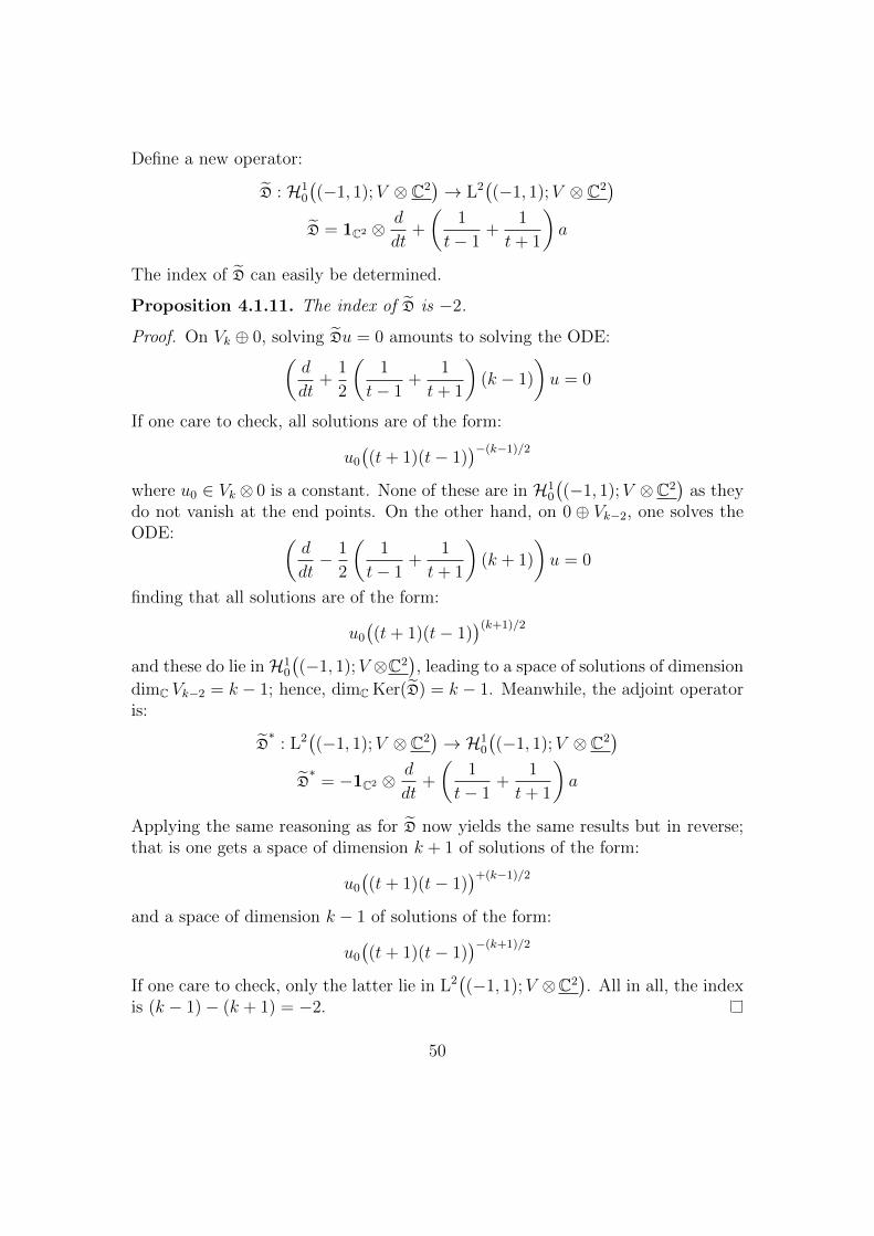
Define a new operator:
D : H10
((−1, 1);V ⊗ C2
)→ L2
((−1, 1);V ⊗ C2
)D = 1C2 ⊗ d
dt+
(1
t− 1+
1
t+ 1
)a
The index of D can easily be determined.
Proposition 4.1.11. The index of D is −2.
Proof. On Vk ⊕ 0, solving Du = 0 amounts to solving the ODE:(d
dt+
1
2
(1
t− 1+
1
t+ 1
)(k − 1)
)u = 0
If one care to check, all solutions are of the form:
u0
((t+ 1)(t− 1)
)−(k−1)/2
where u0 ∈ Vk ⊗ 0 is a constant. None of these are in H10
((−1, 1);V ⊗C2
)as they
do not vanish at the end points. On the other hand, on 0 ⊕ Vk−2, one solves theODE: (
d
dt− 1
2
(1
t− 1+
1
t+ 1
)(k + 1)
)u = 0
finding that all solutions are of the form:
u0
((t+ 1)(t− 1)
)(k+1)/2
and these do lie inH10
((−1, 1);V ⊗C2
), leading to a space of solutions of dimension
dimC Vk−2 = k − 1; hence, dimC Ker(D) = k − 1. Meanwhile, the adjoint operatoris:
D∗
: L2((−1, 1);V ⊗ C2
)→ H1
0
((−1, 1);V ⊗ C2
)D∗
= −1C2 ⊗ d
dt+
(1
t− 1+
1
t+ 1
)a
Applying the same reasoning as for D now yields the same results but in reverse;that is one gets a space of dimension k + 1 of solutions of the form:
u0
((t+ 1)(t− 1)
)+(k−1)/2
and a space of dimension k − 1 of solutions of the form:
u0
((t+ 1)(t− 1)
)−(k+1)/2
If one care to check, only the latter lie in L2((−1, 1);V ⊗C2
). All in all, the index
is (k − 1)− (k + 1) = −2.
50
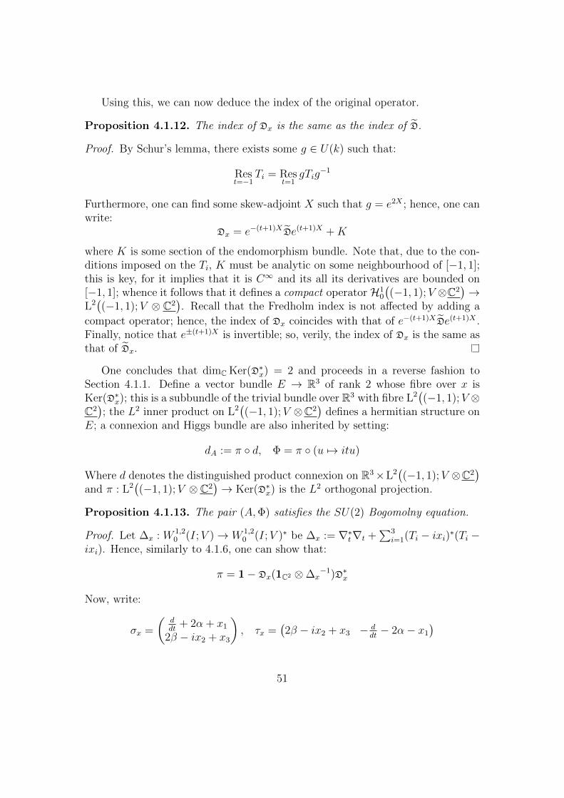
Using this, we can now deduce the index of the original operator.
Proposition 4.1.12. The index of Dx is the same as the index of D.
Proof. By Schur’s lemma, there exists some g ∈ U(k) such that:
Rest=−1
Ti = Rest=1
gTig−1
Furthermore, one can find some skew-adjoint X such that g = e2X ; hence, one canwrite:
Dx = e−(t+1)XDe(t+1)X +K
where K is some section of the endomorphism bundle. Note that, due to the con-ditions imposed on the Ti, K must be analytic on some neighbourhood of [−1, 1];this is key, for it implies that it is C∞ and its all its derivatives are bounded on[−1, 1]; whence it follows that it defines a compact operator H1
0
((−1, 1);V ⊗C2
)→
L2((−1, 1);V ⊗ C2
). Recall that the Fredholm index is not affected by adding a
compact operator; hence, the index of Dx coincides with that of e−(t+1)XDe(t+1)X .Finally, notice that e±(t+1)X is invertible; so, verily, the index of Dx is the same asthat of Dx.
One concludes that dimC Ker(D∗x) = 2 and proceeds in a reverse fashion toSection 4.1.1. Define a vector bundle E → R3 of rank 2 whose fibre over x isKer(D∗x); this is a subbundle of the trivial bundle over R3 with fibre L2
((−1, 1);V ⊗
C2); the L2 inner product on L2
((−1, 1);V ⊗C2
)defines a hermitian structure on
E; a connexion and Higgs bundle are also inherited by setting:
dA := π d, Φ = π (u 7→ itu)
Where d denotes the distinguished product connexion on R3×L2((−1, 1);V ⊗C2
)and π : L2
((−1, 1);V ⊗ C2
)→ Ker(D∗x) is the L2 orthogonal projection.
Proposition 4.1.13. The pair (A,Φ) satisfies the SU(2) Bogomolny equation.
Proof. Let ∆x : W 1,20 (I;V )→ W 1,2
0 (I;V )∗ be ∆x := ∇∗t∇t +∑3
i=1(Ti − ixi)∗(Ti −ixi). Hence, similarly to 4.1.6, one can show that:
π = 1− Dx(1C2 ⊗∆x−1)D∗x
Now, write:
σx =
(ddt
+ 2α + x1
2β − ix2 + x3
), τx =
(2β − ix2 + x3 − d
dt− 2α− x1
)
51

So as to be able to decompose:
Dx =(σx τ ∗x
), D∗x =
(σ∗xτx
)Whence it follows that:
Dx(1C2 ⊗ Fx)D∗x = σxFxσ∗x + τ ∗xFxτx
Further, due to equation (Eq. 4.12), one has:
D∗xDx =
(σ∗xσx σ∗xτxτxσ
∗x τxτ
∗x
)=
(∆x 00 ∆x
)(Eq. 4.13)
It turns out, as in Section 4.1.1, that it is easier to work over R4 in order to be ableto use a complex structure; hence, write B = Φdx0 +A1dx1 +A2dx2 +A3dx3; thus,what must be shown is that the connexion B is ASD. For that end, let L → R4
denote the trivial vector bundle with fibre the Hilbert space L2((−1, 1);V ⊗ C2
);
then, define a Dirac operator on this bundle:
/D′±
: Γ(S± ⊗ L)→ Γ(S∓ ⊗ L)
/D′±
= /D± ± ite0
Where /D is the usual Dirac operator with respect to the product connexion on Land t is to be understood as sending a section f ∈ L2
((−1, 1);V ⊗C2
)to t 7→ tf(t).
In line with Section 4.1.1, write:
/D′+
=√
2(∂ ∂∗
), /D
′−=√
2
(∂∗
∂
)One can see easily that ∂B = π ∂. Now, the operators σx and τx define operatorsσ and τ on the relevant vector bundles over R4 by letting x vary. Then, usingjuxtaposition to denote composition, observe:
∂2B =π∂π∂
=(1− σ∆−1σ∗ − τ ∗∆−1τ)∂(1− σ∆−1σ∗ − τ ∗∆−1τ)∂
=− ∂σ∆−1σ∗∂ − ∂τ ∗∆−1τ ∂
+ σ∆−1σ∗∂σ∆−1σ∗∂ + σ∆−1σ∗∂τ ∗∆−1τ ∂
+ τ ∗∆−1τ ∂σ∆−1σ∗∂ + τ ∗∆−1τ ∂τ ∗∆−1τ ∂
By a direct calculation, one can verify that [∂, σ] = 0 and [∂, τ ] = 0. Using thesefacts, together with ∂2 = 0 and the relations deduced from equation (Eq. 4.13),
52

one can simplify:
=− ∂σ∆−1σ∗∂ − ∂τ ∗∆−1τ ∂
+ σ∆−1σ∗σ∂∆−1σ∗∂ + σ∆−1σ∗∂τ ∗∆−1τ ∂
+ τ ∗∆−1τσ∂∆−1σ∗∂ + τ ∗∆−1∂ττ ∗∆−1τ ∂
=− ∂τ ∗∆−1τ ∂ + σ∆−1σ∗∂τ ∗∆−1τ ∂
=− (1− σ∗∆−1σ)∂τ ∗∆−1τ ∂
=(1− σ∗∆−1σ)∂(1− τ ∗∆−1τ)∂
Now, note that the expression 1 − τ ∗∆−1τ is, in fact, the orthogonal projectiononto the kernel of τ ; since [∂, τ ] = 0, ∂ also commutes with this projection andone concludes:
∂2B = 0
Which is to say that ∂B defines a holomorphic structure on E no matter thecomplex structure chosen for R4. By varying the complex structure on R4, itfollows that B is ASD.
At this point, what remains to be done of the construction is to confirm thatthe asymptotic behaviour of (A,Φ) is as it must be in order to be a monopole ofcharge k; that is, we must verify that YMH(A,Φ) < ∞, |Φ(x)| → 1 and that theeigenbundles of Φ away from some large ball have Chern classes ±k.
For that, we must define yet another operator. Fix x ∈ R3 and set:
D′x : H10
((−1, 1);V ⊗ C2
)→ L2
((−1, 1);V ⊗ C2
)D′x = e−(t+1)XDe(t+1)X + i
3∑i=1
xiei ⊗ 1Ck
Note that Dx = D′x +K for some K smooth in a neighbourhood of [−1, 1]; whenceit follows that the index of D′x coincides with that of Dx (c.f. proposition Propos-ition 4.1.12). Integrating by parts, one can show, for f ∈ H1
0
((−1, 1);V ⊗ C2
)(recall that f vanishes at ±1), that:
〈D∗xDxf, f〉L2 =
∥∥∥∥ ddtf∥∥∥∥2
L2
+
⟨(|x|2 +
∑i
T ∗i Ti
)f, f
⟩L2
≥ |x|2 ‖f‖2L2
Therefore, for sufficiently large |x|, it follows that there is some constant c ∈ Rsuch that 〈D′x
∗D′xf, f〉 ≥ c2|x|2 ‖f‖2
L2 . Which means that D′x∗D′x is also a positive
operator for large r = |x|. Together with the remark above about the index, thisleads to dimC Ker(D′x
∗) = 2.
53

Use Px to denote the orthogonal projection onto the kernel of D′x∗; then, let
Gx be the Green’s function of D′x; so D′xGx = 1− Px and GxD′x = 1. Notice that:
‖f − Pxf‖2 = ‖D′xGxf‖2= 〈D′x
∗D′xGxf,Gxf〉 ≥ c2r2 ‖Gxf‖2
So:‖Gxf‖ cr ≤ ‖f − Pxf‖ ≤ ‖f‖
Which is to say that:
‖Gx‖ ≤ 1/cr, ‖G∗x‖ ≤ 1/cr (Eq. 4.14)
Consider a solution f to D∗xf = 0. Since G∗xD′∗ = 1− Px, one has:
f − Pxf = G∗x(D∗x −K∗)f = −G∗xK∗f
Therefore, one can find some constant c′ ∈ R such that:
‖f − Pxf‖ ≤c′
r‖f‖ (Eq. 4.15)
Which means that we can approximate, up to order r−1, solutions to D∗f = 0 bysolutions to D′∗f = 0.
We now proceed to find a basis of solutions for D′∗f = 0. Fix a u ∈ R3 suchthat |u| = 1. Then, u generates a circle subgroup of SU(2) by exponentiating∑3
i=1 uiei ∈ su(2); furthermore, this subgroup is a maximal toral subgroup and,with respect to it, one can decompose any representation as a direct sum of weightspaces. We are interested in the representation V1 ⊗ Vk−1 because of the form ofthe operator D which contains the term a =
∑3i=1 ei⊗ai which acts via this repres-
entation. Recall that V1⊗ Vk−1∼= Vk⊕ Vk−2 as su(2) representations; therefore, by
knowledge of the representation theory of su(2), one knows that the weight spacedecomposition has weights:
−k,−(k − 2), . . . , (k − 2), k in Vk ⊕ 0
−(k − 2),−(k − 4), . . . , (k − 4), (k − 2) in 0⊕ Vk−2
Each weight, in both cases, has multiplicity 1; thus, one sees that the weight spacesof weight ±k have dimension 1; all others have dimension 2. Now, the operatorD′u contains the term i
∑3i=1 uiei ⊗ 1Vk−1
; the action of this term commutes withthe action of a; whence it follows that it preserves the weight space decompositionabove; furthermore, since the weight spaces of weight ±k are one dimensional, itmust act as a scalar on each of these two weight spaces. The scalars are, in fact,respectively ±1; this can be seen by noting:(
i
3∑i=1
uiei ⊗ 1Vk−1
)2
= 1V1⊗Vk−1
54
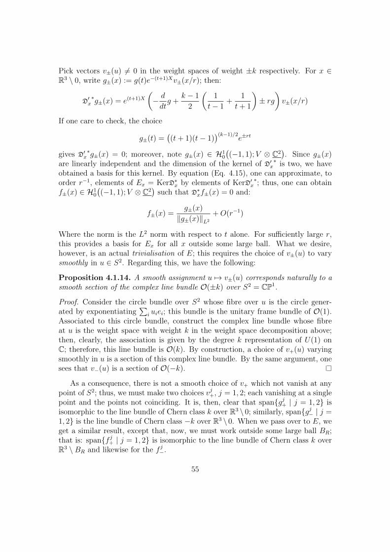
Pick vectors v±(u) 6= 0 in the weight spaces of weight ±k respectively. For x ∈R3 \ 0, write g±(x) := g(t)e−(t+1)Xv±(x/r); then:
D′x∗g±(x) = e(t+1)X
(− d
dtg +
k − 1
2
(1
t− 1+
1
t+ 1
)± rg
)v±(x/r)
If one care to check, the choice
g±(t) =((t+ 1)(t− 1)
)(k−1)/2e±rt
gives D′x∗g±(x) = 0; moreover, note g±(x) ∈ H1
0
((−1, 1);V ⊗ C2
). Since g±(x)
are linearly independent and the dimension of the kernel of D′x∗ is two, we have
obtained a basis for this kernel. By equation (Eq. 4.15), one can approximate, toorder r−1, elements of Ex = KerD∗x by elements of KerD′x
∗; thus, one can obtainf±(x) ∈ H1
0
((−1, 1);V ⊗ C2
)such that D∗xf±(x) = 0 and:
f±(x) =g±(x)
‖g±(x)‖L2
+O(r−1)
Where the norm is the L2 norm with respect to t alone. For sufficiently large r,this provides a basis for Ex for all x outside some large ball. What we desire,however, is an actual trivialisation of E; this requires the choice of v±(u) to varysmoothly in u ∈ S2. Regarding this, we have the following:
Proposition 4.1.14. A smooth assignment u 7→ v±(u) corresponds naturally to asmooth section of the complex line bundle O(±k) over S2 = CP1.
Proof. Consider the circle bundle over S2 whose fibre over u is the circle gener-ated by exponentiating
∑i uiei; this bundle is the unitary frame bundle of O(1).
Associated to this circle bundle, construct the complex line bundle whose fibreat u is the weight space with weight k in the weight space decomposition above;then, clearly, the association is given by the degree k representation of U(1) onC; therefore, this line bundle is O(k). By construction, a choice of v+(u) varyingsmoothly in u is a section of this complex line bundle. By the same argument, onesees that v−(u) is a section of O(−k).
As a consequence, there is not a smooth choice of v+ which not vanish at anypoint of S2; thus, we must make two choices vj+, j = 1, 2; each vanishing at a singlepoint and the points not coinciding. It is, then, clear that spangj+ | j = 1, 2 isisomorphic to the line bundle of Chern class k over R3 \ 0; similarly, spangj− | j =1, 2 is the line bundle of Chern class −k over R3 \ 0. When we pass over to E, weget a similar result, except that, now, we must work outside some large ball BR;that is: spanf j+ | j = 1, 2 is isomorphic to the line bundle of Chern class k overR3 \BR and likewise for the f j−.
55
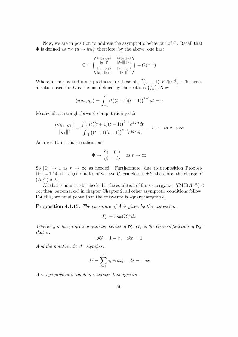
Now, we are in position to address the asymptotic behaviour of Φ. Recall thatΦ is defined as π (u 7→ itu); therefore, by the above, one has:
Φ =
〈itg+,g+〉‖g+‖2〈itg+,g−〉‖g+‖‖g−‖
〈itg−,g+〉‖g−‖‖g+‖
〈itg−,g−〉‖g−‖2
+O(r−1)
Where all norms and inner products are those of L2((−1, 1);V ⊗ C2
). The trivi-
alisation used for E is the one defined by the sections f±; Now:
〈itg±, g∓〉 =
∫ 1
−1
it((t+ 1)(t− 1)
)k−1dt = 0
Meanwhile, a straightforward computation yields:
〈itg±, g±〉‖g±‖2 =
∫ 1
−1it((t+ 1)(t− 1)
)k−1e±2rtdt∫ 1
−1
((t+ 1)(t− 1)
)k−1e±2rtdt
−→ ±i as r →∞
As a result, in this trivialisation:
Φ→(i 00 −i
)as r →∞
So |Φ| → 1 as r → ∞ as needed. Furthermore, due to proposition Proposi-tion 4.1.14, the eigenbundles of Φ have Chern classes ±k; therefore, the charge of(A,Φ) is k.
All that remains to be checked is the condition of finite energy, i.e. YMH(A,Φ) <∞; then, as remarked in chapter Chapter 2, all other asymptotic conditions follow.For this, we must prove that the curvature is square integrable.
Proposition 4.1.15. The curvature of A is given by the expression:
FA = πdxGG∗dx
Where πx is the projection onto the kernel of D∗x; Gx is the Green’s function of Dx;that is:
DG = 1− π, GD = 1
And the notation dx, dx signifies:
dx =3∑i=1
ei ⊗ dxi, dx = −dx
A wedge product is implicit wherever this appears.
56
Proof. By definition, the curvature is FA = πdπd. The key facts in this proof arethe following:
[d,D] = dx, [d,D∗] = dx
These are trivially verified. Hence, consider:
πdxGG∗dx = π[d,D]GG∗[d,D∗]
= π(dD− Dd)GG∗(dD∗ − D∗d)
The term with D∗ on the right vanishes as we are acting on elements of the kernelof D∗; whereas the term with πD on the left vanishes because π is the orthogonalprojection onto the kernel of D∗ which is the orthogonal complement of the imageof D. What remains is:
= −πdDGG∗D∗d= −πd(1− π)(1− π)d
= πdπd
= FA
To conclude, notice that the bound obtained for the Green’s function of D′ in(Eq. 4.14) and the ability to approximate the kernel of D by the kernel of D′ asshown in (Eq. 4.15) imply that we also have a bound on the norms of the Green’sfunction of D:
‖G‖ ≤ 1/cr, ‖G∗‖ ≤ 1/cr
So:
‖FA‖ ≤ ‖π‖ ‖dx‖ ‖G‖ ‖G∗‖ ‖dx‖ = ‖G‖ ‖G∗‖ ≤ 1
c2r2
Where these norms are being thought of as the operator norms of bounded linearmaps. Since we work in R3 this places FA in L2 and
YMH(A,Φ) =
∫R3
‖FA‖2 + ‖dAΦ‖2 <∞
In summary, we have proved:
Theorem 4.1.16. The pair (A,Φ) where A is the connexion on the hermitianbundle E = KerD∗ defined as dA = π d and Φ is the endomorphism of E definedas π (u 7→ itu) is an SU(2) monopole of charge k.
The construction presented in this section is the inverse of the construction ofNahm data from a monopole presented in section Section 4.1.1. This is certainlysomething that must be checked, but, due to time constraints, the proof was leftout of this project; we refer the reader to [Nak93] for details.
57
4.2 Singular Monopoles and Nahm’s Equations
The Nahm transform between SU(2) monopoles and solutions of Nahm’s equationsis a specific case of a more general collection of correspondences between invariantinstantons on four-manifolds. One particular example of this type of correspond-ence should be given by the case of singular monopoles on R3. In this section wewill investigate this correspondence.
The correspondence we will investigate is between Dirac monopoles on R3 asdescribed in Section 2.3 and solutions of Nahm’s equations given by the followingdata:
1. A Hermitian bundle V of rank k over (0,∞) where k = k1 + · · · + kn is thesum of charges of the Dirac monopoles, and
2. a unitary connection ∇t on V and three skew-Hermitian endomorphismsT1, T2, T3 satisfying Nahm’s equations, such that
(a) The Tα are analytic for all s ∈ (0,∞),
(b) as s → 0 the residues of the Tα define an irreducible representation ofsu(2), and
(c) as s→∞, the operators Tα approach a commuting triple given by
i diag((p1)α, . . . , (p1)α︸ ︷︷ ︸k1times
, . . . , (pn)α, . . . , (pn)α︸ ︷︷ ︸kntimes
)
where pi = ((pi)1, (pi)2, (pi)3) gives the coordinates of a singularity ofthe corresponding monopole with charge ki.
In the case of SU(2) monopoles the bundle V → (−1, 1) upon which the Nahmdata correponding to the monopole lived was constructed as the kernel of a twistedDirac operator on R3. This same approach can be attempted in the case of Diracmonopoles. However, the presence of the singularities requires that one appliesthe techniques of b-geometry and scattering calculus, as detailed for example in[Mel93].
In particular, let Φs denote the Higgs field of a Dirac monopole of mass s, givenexplicitly by
Φs := i
(s+
n∑i=1
ki2|x− pi|
),
where the pi denote the n singularities of Φ1 and the ki are the charges of thesesingularities. We will often denote the distance function |x− pi| on R3 by ri.
58

As in the case of SU(2) monopoles, we are interested in the operator
/DA,s := /DA + Φs
where A is the connection form corresponding to the Higgs field. Again we havethat the formal adjoint of /DA,s is
/D∗A,s = /DA − Φs
due to the skew-Hermiticity of Φs, and by the Weitzenbock formula we have
/D∗A,s
/DA,s = ∇∗A∇A − Φ2s
which is a positive operator.
Remark 4.2.1. A special case of this is where we have a single singularity at theorigin. Here, we have a very manageable exact formula for the Dirac operator,namely
D∗A,s =
(i(∂∂r− s− k−2
2r
)1r/D−
1r/D
+ −i(∂∂r
+ s+ k+22r
)) .We can directly try to compute the kernel of this operator.
If we start by looking for functions of the form g(r)f(θ), where we view R3\0as S2×R+ and g a function on R and f a section of the bundle O(k−1)⊕O(k+1)over S2 = CP1, then we can easily check that we have a k-dimensional space ofsolutions, given by (e−srr
k−22 f, 0), where f ∈ H0(CP,O(k − 1)).
Using some further argument involving decomposing the spaces of sections overthe sphere into eigenspaces of the Laplacian one would attempt to prove that theseare indeed all the solutions.
The general case, however, is more complicated. We can, however, write someasymptotic behaviours (cf. (Eq. 4.8)) The behaviour of our operators near infinitycan be written as
/DA,s =
(i(∂∂r
+ s+ k+22r
)1r/D−
1r/D
+ −i(∂∂r− s− k−2
2r
))+O(r−2), (Eq. 4.16)
/D∗A,s =
(i(∂∂r− s− k−2
2r
)1r/D−
1r/D
+ −i(∂∂r
+ s+ k+22r
))+O(r−2), (Eq. 4.17)
and the behaviour near the singularity pi is given by
/DA,s =
i( ∂∂ri
+ ki+22ri
)1ri/D−
1ri/D
+ −i(
∂∂ri− ki−2
2ri
)+O(1) (Eq. 4.18)
/D∗A,s =
i( ∂∂ri− ki−2
2ri
)1ri/D−
1ri/D
+ −i(
∂∂ri
+ ki+22ri
)+O(1) (Eq. 4.19)
59
(note that here the s is absorbed into the O(1), since it is a constant).Now, in order to define the Nahm data, we want to know what the kernels of
these operators are. In order to do this, we will need to apply ideas from b- andsc-geometry. In the following sections we will give a concise introduction to theseideas and explain how the apply to our case.
The underlying idea to both is the following. Let M be a smooth manifold withboundary. A smooth function x on M such that x|∂M = 0, x 6= 0 away from ∂M ,and dx|∂M 6= 0 is called a boundary-defining function on M . In a neighbourhoodof a boundary point of M , one may use x to define a local coordinate system(x, y1, . . . , yn) where (y1, . . . , yn) are local coordinates on the boundary ∂M .
Consider R3\P where P is the finite set of points where Φs has singularities.One may perform the real blowup of this space at each point pi ∈ P and at ∞ toobtain a compact manifold M = R3\P with boundary, such that
∂M = ∂∞M t⊔pi∈P
∂iM,
where ∂∞M ∼= S2 is a sphere at ∞, and ∂iM ∼= S2 is a sphere about each singu-larity pi of Φs.
Furthermore, in our case, xi := riri+1
is a boundary defining function for each
∂iM and x∞ := 1r
(properly cut off for small r) is a boundary defining functionfor ∂∞M . We denote x = Π ri
1+ri, which is a boundary defining function for all the
boundaries at the singularities (not to confuse the notation with the one for thecoordinates on R3).
4.2.1 b-Geometry and the case s = 0
Given M a manifold with boundary, construct the b-vector fields by
Vectb(M) := X ∈ Γ(M,TM) | X is tangent to ∂M.
If M has a boundary-defining function x, then in local coordinates near the bound-ary a b-vector field is a smooth linear combination of
x∂
∂x,∂
∂y1, . . . ,
∂
∂yn.
Remark 4.2.2. If one makes a change of variables t := log x then ∂∂t
= x ∂∂x
andthe boundary ∂M = x = 0 corresponds to the limit as t → −∞. Further,the local coordinate system of (t, y1, . . . , yn) identifies a small neighbourhood of∂M in M with the infinite cylinder ∂M × (−∞, a) for some a ∈ R. In this sense,b-geometry is the study of differential operators on manifolds with boundary byviewing the boundary as a cylindrical end (and considering vector fields which areasymptotically translation invariant).
60
These b-vector fields are first-order differential operators on M , and analog-ously to the regular definition of differential operators, one may define the algebraDiffdb(M) of b-differential operators of order d on M .
Using the differential operator x ∂∂x
instead of ∂∂x
near the boundary, one mayalso analogously define the b-Sobolev spaces Hk
b of M . These Sobolev spaces relyon the usual metric on the manifold. In a way, a function is in Hm
b if its first kb-derivatives are in (usual) L2. Hence, if P is a b-differential operator of order d,then
P : Hmb → Hm−d
b
for all k.Locally, a b-differential operator of order m has the form
P = p
(x, y;x
∂
∂x,∂
∂y1, . . . ,
∂
∂yn
)= p0(x, y) +
d∑i=1
pi(x, y, x∂
∂x,∂
∂y1, . . . ,
∂
∂yn),
where p is some polynomial of degree d in the given arguments, and pi is homo-genous of degree i.
Just as in the case of regular differential operators, one may define the b-symbolfrom the highest order term of P by
σb(P )(x, y, ξ, η1, . . . , ηn) := pd(x, y, ξ, η1, . . . , ηn)
for formal variables ξ, ηj corresponding to x ∂∂x
and the ∂∂yj
. A b-differential operator
is b-elliptic when σb(P ) is invertible for (ξ, ηj) 6= 0.Unlike in the case of regular differential operators on a smooth manifold M , it is
not true that a b-elliptic b-differential operator is Fredholm on b-Sobolev spaces. Inthe setting of b-geometry there are obstructions to Fredholmness that are detectedby the normal operator of P . Define the normal operator N(P ) by
N(P ) :=d∑i=0
pi(0, y;x∂
∂x,∂
∂yj).
A complex number α is an indicial root of N(P ) if there exists a non-zero functionu on ∂M such that
N(P )(xαu(y)) = 0.
In this case one has the following theorem.
61

Theorem 4.2.3 (See [Mel93, §5.17], or [LMO85]). If P is a b-elliptic b-differentialoperator and δ ∈ R is not the real part of any indicial root of N(P ), then
P : xδHmb (M,E)→ xδHm−d
b (M,E)
is Fredholm. Here f ∈ xδHmb if x−δf ∈ Hm
b . Denote the index of P at weight δ byInd(P, δ).
In addition to this result, there is a wall-crossing formula as the parameter δpasses across the indicial roots of N(P ).
Theorem 4.2.4 (See [LMO85]). If δ1 < α < δ2 and α is the only indicial root ofN(P ) between δ1 and δ2 which are not indicial roots, then
Ind(P, δ2)− Ind(P, δ1) = dimu | N(P )(xαu(y)) = 0.
Finally one may define the b-adjoint of a b-differential operator P by integrationwith respect to a b-volume form on M . If
P : xδHmb (M,E)→ xδHm−d
b (M,E)
thenP ∗ : x−δHm
b (M,E)→ x−δHm−db (M,E)
and kerP ∗ = cokerP , and Ind(P ∗,−δ) = − Ind(P, δ). This allows us to computethe index of an operator if we know its relationship to it’s dual. For example, if Pis b-self-adjoint, then we would have the following.
Theorem 4.2.5 (See [LMO85]). If P ∗ = P then
2 Ind(P, δ) = Ind(P, δ)− Ind(P,−δ) =∑−δ<α<δ
dimu | N(P )(xαu(y)) = 0
where α runs over all indicial roots between −δ and δ.
For more details on the various constructions in b-geometry, including of theb-tangent bundle, b-metrics, b-integrals, and various other natural differential-geometric and analytic constructions, we refer to the seminal [Mel93], particularlyChapters 2, 4, and 5.
As it turns out, this setting will be adequate for studying our Dirac operatorsin the particular case where the mass is s = 0. This is the approach considered bySinger in the unpublished notes [Sin00], which we follow here.
Indeed, we see that the behaviours of xi /DA,0 and xi /D∗A,0 near the singularities
and x−1∞ /DA,0 and x−1
∞ /D∗A,0 near infinity are precisely the behaviours of b-operators
(see (Eq. 4.16), (Eq. 4.17), (Eq. 4.18) and (Eq. 4.19)). Furthermore, one can
62

easily see that they are b-elliptic. This means that they will be Fredholm operators
/DA,0, /D∗A,0 : xµxδ∞Hm
b (M, /S ⊗ E)→ xµ−1xδ+1∞ Hm−1
b (M, /S ⊗ E). (Eq. 4.20)
In fact, we will think of µ as a kind of multi-index, in the sense that we havex(µ1,...,µn) = Πxµii (and µ− 1 refers to reducing each component by 1).
Let us then look at the normal operators. Consider, for and integer κ > 0 anda real number λ, the operator
Nλκ =
(i(α + 1 + λκ
2
)/D−
/D+ −i
(α + 1− λκ
2
)) ,acting on sections of O(κ− 1)⊕O(κ+ 1) of CP1.
N1k and N−1
k are the normal operators for x−1∞ /DA,0 and x−1
∞ /D∗A,0, respectively,
at the sphere at infinity, where k the sum of charges (and acting on sections of theform xαu). Analogously, taking κ to be ki would give us the normal operators ofxi /DA,0 and xi /D
∗A,0. Therefore, we are interested in computing the indicial roots of
these operators.Recall that /D
+and /D
−are 2∂κ and 2∂
∗κ, the Dolbeault operator on the holo-
morphic bundle O(κ−1) and its dual (on O(κ+1) =∧
0,1⊗O(κ−1)) on S2 = CP1.If α is an indicial root of this operator, then we will be have u+ and u−, (smooth)sections of O(κ− 1) and O(κ+ 1), respectively, so that
i
(α + 1 +
λκ
2
)u+ + 2∂
∗u− = 0, (Eq. 4.21)
−i(α + 1− λκ
2
)u− + 2∂u+ = 0. (Eq. 4.22)
We want to compute the dimension of the space of solutions of this system. Inorder to do so, we need to know the eigenvalues of the Laplacian 4∂
∗κ∂κ on CP1.
Lemma 4.2.6. Let ∂κ denote the Dolbeault operator on O(κ) ⊗ /S+ → CP1 for
κ > 0, and let ∇κ denote the Chern connection. The eigenvalues of the DolbeaultLaplacian
4∂∗κ∂κ
are given by`(`+ κ) | ` ∈ Z≥0.
Proof. This follows from the Weitzenbock formula for the twisted Dirac operatoron O(κ)⊗ /S+
. Recall that /S+ ∼= O(−1). It is shown in [Kuw82, Thm. 5.1] that the
63
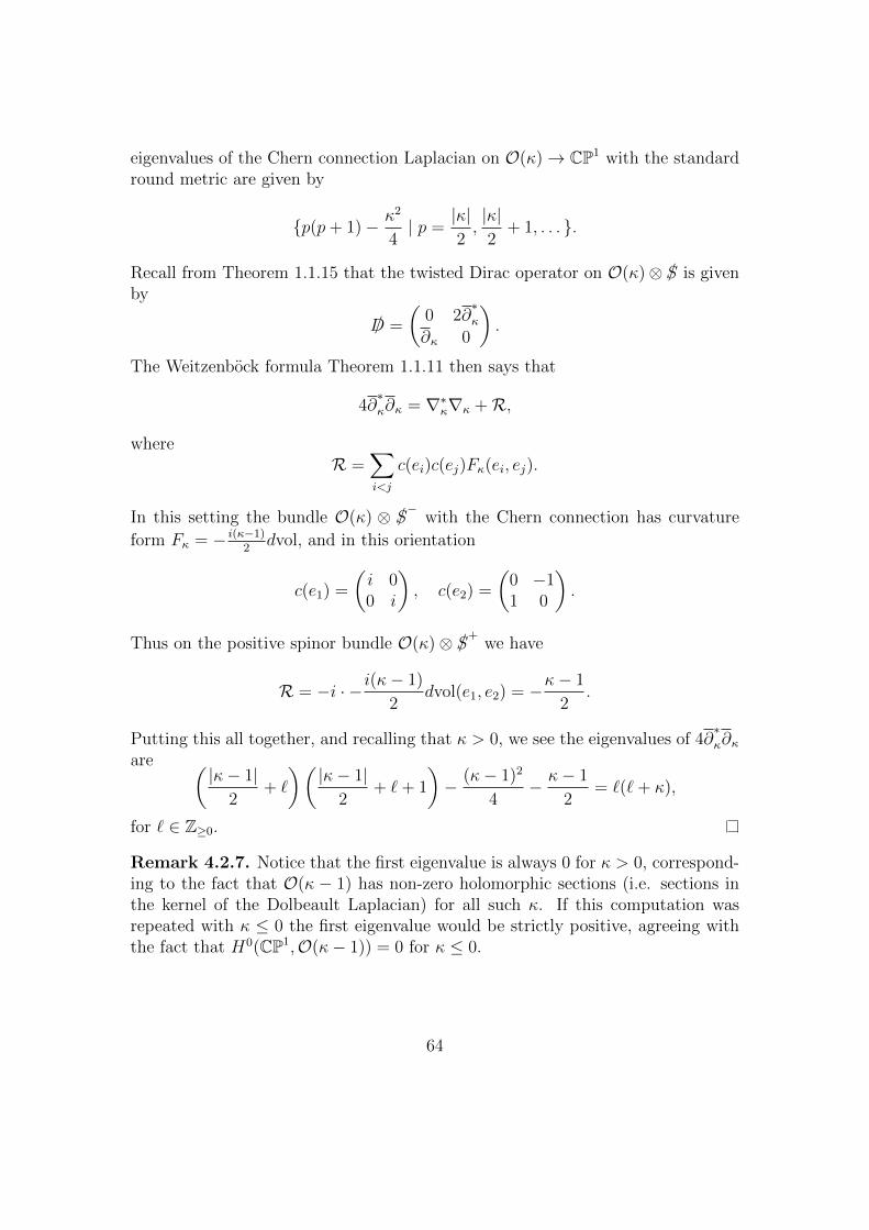
eigenvalues of the Chern connection Laplacian on O(κ)→ CP1 with the standardround metric are given by
p(p+ 1)− κ2
4| p =
|κ|2,|κ|2
+ 1, . . . .
Recall from Theorem 1.1.15 that the twisted Dirac operator on O(κ)⊗ /S is givenby
/D =
(0 2∂
∗κ
∂κ 0
).
The Weitzenbock formula Theorem 1.1.11 then says that
4∂∗κ∂κ = ∇∗κ∇κ +R,
whereR =
∑i<j
c(ei)c(ej)Fκ(ei, ej).
In this setting the bundle O(κ) ⊗ /S−
with the Chern connection has curvature
form Fκ = − i(κ−1)2
dvol, and in this orientation
c(e1) =
(i 00 i
), c(e2) =
(0 −11 0
).
Thus on the positive spinor bundle O(κ)⊗ /S+
we have
R = −i · − i(κ− 1)
2dvol(e1, e2) = −κ− 1
2.
Putting this all together, and recalling that κ > 0, we see the eigenvalues of 4∂∗κ∂κ
are (|κ− 1|
2+ `
)(|κ− 1|
2+ `+ 1
)− (κ− 1)2
4− κ− 1
2= `(`+ κ),
for ` ∈ Z≥0.
Remark 4.2.7. Notice that the first eigenvalue is always 0 for κ > 0, correspond-ing to the fact that O(κ − 1) has non-zero holomorphic sections (i.e. sections inthe kernel of the Dolbeault Laplacian) for all such κ. If this computation wasrepeated with κ ≤ 0 the first eigenvalue would be strictly positive, agreeing withthe fact that H0(CP1,O(κ− 1)) = 0 for κ ≤ 0.
64

We now return to the solutions of our system of equations. By applying 2∂∗
to(Eq. 4.22) and substituting with (Eq. 4.21), we would get
4∂∗κ∂κu =
((α + 1)2 −
(λκ
2
)2)u. (Eq. 4.23)
This means that, if the original system is to have any solution, we must have that
(α + 1)2 −(λκ2
)2must be equal to some eigenvalue `(`+ κ), for some ` ∈ Z≥0. In
other words, α = −√(
λκ2
)2+ `(`+ κ)− 1 or α =
√(λκ2
)2+ `(`+ κ)− 1.
If ` 6= 0, this corresponds to a non-zero eigenvalue, and a solution to (Eq. 4.23)will always give rise to solutions of the original system. Therefore, for all thesevalues, α is an actual indicial root (the dimension of the space of solutions can becomputed to be κ+ 2`, but this will not be relevant to our case).
However, the case ` = 0 is slightly more complicated, since we will not alwaysbe able to go back to a solution of the original system. Hence, let us look atthis case more closely. Firstly, we see that this corresponds to the indicial rootsα = λκ
2− 1 and α = −λκ
2− 1, so we can take both cases separately. Also, for now,
let λ 6= 0.Hence, let us first look at α = λκ
2− 1. In this case, the system becomes
2∂∗u− = iλκu+,
2∂u+ = 0.
By applying 2∂ to the first equation, we get that ∂∂∗u− = 0, which implies that
u− = 0, given that it’s a section of O(κ + 1) (with κ > 0). Hence, we must alsohave u+ = 0, so there are no non-trivial solutions. Therefore, this is not an actualindicial root.
If α = −λκ2− 1, then the system becomes
2∂∗u− = 0,
2∂u+ = −iλκu−.
This implies that u− = 0, so our solutions will precisely be given by holomorphicsections of O(κ− 1), of which there is precisely a κ-dimensional space.
If λ = 0, then the two previous cases are the same, and are simply
2∂∗u− = 0,
2∂u+ = 0,
so again we have a κ-dimensional space of solutions.
65
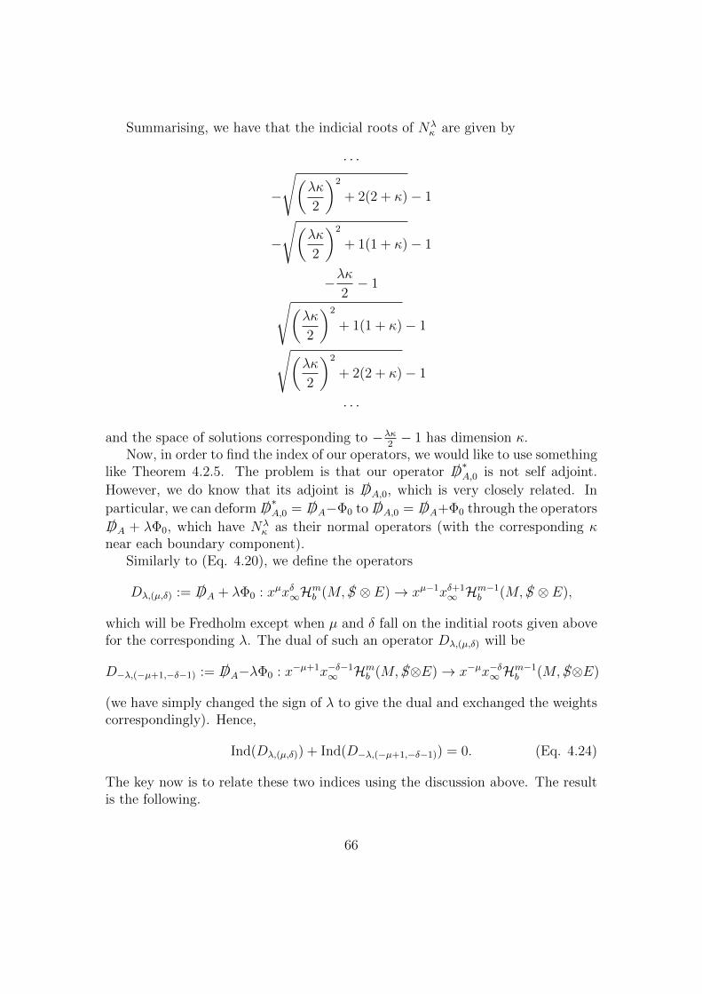
Summarising, we have that the indicial roots of Nλκ are given by
· · ·
−
√(λκ
2
)2
+ 2(2 + κ)− 1
−
√(λκ
2
)2
+ 1(1 + κ)− 1
−λκ2− 1√(
λκ
2
)2
+ 1(1 + κ)− 1√(λκ
2
)2
+ 2(2 + κ)− 1
· · ·
and the space of solutions corresponding to −λκ2− 1 has dimension κ.
Now, in order to find the index of our operators, we would like to use somethinglike Theorem 4.2.5. The problem is that our operator /D
∗A,0 is not self adjoint.
However, we do know that its adjoint is /DA,0, which is very closely related. In
particular, we can deform /D∗A,0 = /DA−Φ0 to /DA,0 = /DA+Φ0 through the operators
/DA + λΦ0, which have Nλκ as their normal operators (with the corresponding κ
near each boundary component).Similarly to (Eq. 4.20), we define the operators
Dλ,(µ,δ) := /DA + λΦ0 : xµxδ∞Hmb (M, /S ⊗ E)→ xµ−1xδ+1
∞ Hm−1b (M, /S ⊗ E),
which will be Fredholm except when µ and δ fall on the inditial roots given abovefor the corresponding λ. The dual of such an operator Dλ,(µ,δ) will be
D−λ,(−µ+1,−δ−1) := /DA−λΦ0 : x−µ+1x−δ−1∞ Hm
b (M, /S⊗E)→ x−µx−δ∞Hm−1b (M, /S⊗E)
(we have simply changed the sign of λ to give the dual and exchanged the weightscorrespondingly). Hence,
Ind(Dλ,(µ,δ)) + Ind(D−λ,(−µ+1,−δ−1)) = 0. (Eq. 4.24)
The key now is to relate these two indices using the discussion above. The resultis the following.
66

Proposition 4.2.8. Suppose that
µ =
(k1 + 1
2− ε, . . . , kn + 1
2− ε), δ =
k + 1
2+ ε,
for some small enough ε > 0. Then,
Ind(D−1,(µ,δ))− Ind(D1,(−µ+1,−δ−1)) = 2k
(where k, k1, . . . , kn are the charges of (A,Φ)).
Proof. The proof of this proposition is best explained through the diagrams presen-ted in Figures 4.1 and 4.2. Indeed, given the weights of our spaces, that will de-termine which indicial roots fall into the domain near each boundary component.In the figures, we represent with a thick grey line the interval of possible indicialroots that fall into the domains. The indicial roots which actually exist (depend-ing on λ) are represented by the curves and dots. The straight line in the middlerepresents the indicial root −λκ
2− 1, which we know to correspond to a space of
dimension κ.Therefore, we see that in all the boundary components, as we deform our
operator we are going to leave out a κ-dimensional space corresponding to theindicial roots. Therefore, the index will decrease by all of these contributions. Thetotal contributions are k + k1 + · · ·+ kn = k + k = 2k.
Corollary 4.2.9. The index of the Dirac operator
/D∗A,0 : xµxδ∞Hm
b (M, /S ⊗ E)→ xµ−1xδ+1∞ Hm−1
b (M, /S ⊗ E)
is k, where µ and δ are like in Proposition 4.2.8.
Proof. This is a direct consequence of Proposition 4.2.8 and (Eq. 4.24).
4.2.2 sc-Geometry and the case s > 0
In addition to b-geometry, we will also be interested in the so-called scatteringcalculus, or sc-geometry, also pioneered by Melrose. See [Mel08, Ch. 7] or [Mel95]for more details on the constructions in this section, which we summarise.
The sc-geometry is constructed parallel to b-geometry as follows. Again letM be a manifold with boundary and x a boundary-defining function. Define thescattering sc-vector fields by Vectsc(M) := xVectb(M). That is, sc-vector fieldsare smooth linear combinations of
x2 ∂
∂x, x
∂
∂y1, . . . , x
∂
∂yn
near ∂M .
67
Remark 4.2.10. Let r := 1x. Then −x2 ∂
∂x= ∂
∂rand x ∂
∂yi= 1
r∂∂yi
. This is the localmodel for a Euclidean coordinate system, as opposed to the b-geometry in whichthe boundary is viewed as a cylindrical end. In this sense sc-calculus is the methodof analysis on manifolds with boundary by viewing the boundary as a Euclideanlimit.
Just as in the b-geometry case, the sc-vector fields allow one to define sc-differential operators Diffdsc(M) of order d. Notice that although Vectsc(M) =xVectb(M), it is not the case that Diffdsc(M) = xDiffdb(M). Indeed x2 ∂
∂x+ 1 =
x(x ∂∂x
+ 1x
)∈ Diff1
sc(M) but is clearly not in xDiff1b(M).
Again one may define the sc-Sobolev spaces Hmsc and the sc-symbol σsc(P ) of
an sc-differential operator by the same expressions as in the b-geometry case. Thenotion of sc-ellipticity is defined in the same way.
Again define the normal operator N(P ) of a scattering operator P by
N(P ) :=d∑i=0
pi(0, y, ξ, η1, . . . , ηn).
We say P is fully elliptic if σsc(P ) is invertible for (ξ, ηj) 6= 0 for all (x, y) and N(P )is invertible for all (ξ, ηj). In this setting there is a divergence with b-geometry,and we have the following theorem.
Theorem 4.2.11 (See [Mel95, §6.5]). If P is a fully elliptic sc-differential operatorof order d, then
P : xδHmsc → xδHm−d
sc
is Fredholm for all m, δ and the index of P is independent of the choice of m, δ.Furthermore
kerP ⊂⋂δ,m
xδHmsc.
Now, if we look back at the asymptotic behaviour of our Dirac operators nearinfinity ((Eq. 4.16) and (Eq. 4.17)), we see that, if s > 0, they behave preciselylike fully elliptic sc-operators at the boundary component ∂∞M (to see this moreconcretely, we need to consider the symbol of the Dolbeault Laplacian and checkthat the normal operator is always invertible).
Hence, whereas before we were only able to consider the case s = 0, now wecan study the case s > 0, which is, in fact, the one that interests us, since it ishere that we will want to define the Nahm data.
Out operator, however, is not a b-operator or an sc-operator, since it behavesdifferently at different components of the boundary. However, we can consider amix of these two kinds of geometry in order to study this case.
68

We start by noting that all the concepts of b- and sc-geometry (vector fields,ellipticity, Sobolev spaces, etc.) only differ from the usual ones in the behaviournear the boundary. That is, in the interior all the notions coincide. Therefore, wecan consider consider something which we could call bsc-geometry, which wouldbe the exact analogous, but imposing b-behaviour near some components of theboundary, and sc behaviour on other components. In the setting of the previoussection, we would like to consider bsc-geometry in the sense that we impose b-behaviour near ∂iM for all i but sc-behaviour near ∂∞M . In this sense, our Diracoperator is a fully elliptic bsc-operator between Sobolev spaces with the appropriateweights, and therefore we would expect it to be Fredholm.
Now, we could try to compute the index using a similar technique to the one weused before. The problem, however, arises when we deform the operators, since atan intermediate point they will cease to be fully elliptic (in the scattering sense).The contribution from the singularities would be the same as before, but we wouldneed a wall-crossing formula for the situation where an sc-operator ceases to befully elliptic. If this gave us another contribution of k, then we would have ourresult.
Another way to tackle this would be by considering the following principle: wehave deduced from the previous section that, if we have no mass, then the index isnot affected by whether there are several singularities or whether all the charge is ata single point. On the other hand, the addition of mass affects only the behaviourtowards infinity (since, recall, the behaviour near the singularities was dictated byxiD
∗A,s, where multiplying by xi made the mass become irrelevant). Therefore, if
we had the case of a monopole with mass, but with all charge concentrated at apoint, changing this to the general situation where we have multiple singularitiesshould not have an impact on the index. This is precisely the case discussed inRemark 4.2.1.
4.2.3 Limit of Nahm Data
In order to determine the behaviour of the Nahm data near the limits, we wouldneed to have a model, similar to the case of SU(2) monopoles (cf. (Eq. 4.9)).In analogy with the previous case, we would expect that the limit as s → 0 bedictated by the behaviour near of the solutions for large r, and we would expect asimilar formula. In the limit s → ∞, however, the limit would be determined bythe behaviour of the solutions near the singularities, where we would also expectsolutions of the same form. In what follows we will study what these limits wouldbe given these possible models. Note, in particular, that these model solutions areconsistent with the weights defined in the previous sections for the domains of theDirac operator.
69
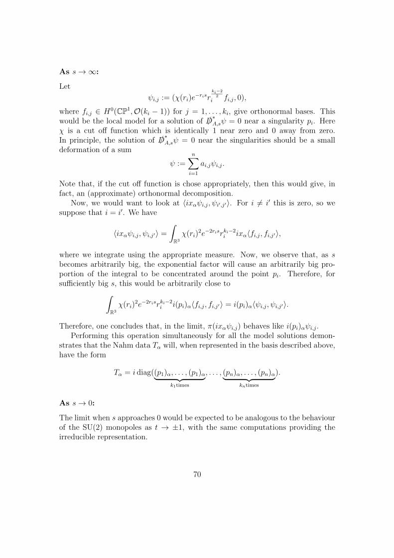
As s→∞:
Let
ψi,j := (χ(ri)e−risr
ki−2
2i fi,j, 0),
where fi,j ∈ H0(CP1,O(ki − 1)) for j = 1, . . . , ki, give orthonormal bases. Thiswould be the local model for a solution of /D
∗A,sψ = 0 near a singularity pi. Here
χ is a cut off function which is identically 1 near zero and 0 away from zero.In principle, the solution of /D
∗A,sψ = 0 near the singularities should be a small
deformation of a sum
ψ :=n∑i=1
ai,jψi,j.
Note that, if the cut off function is chose appropriately, then this would give, infact, an (approximate) orthonormal decomposition.
Now, we would want to look at 〈ixαψi,j, ψi′,j′〉. For i 6= i′ this is zero, so wesuppose that i = i′. We have
〈ixαψi,j, ψi,j′〉 =
∫R3
χ(ri)2e−2risrki−2
i ixα〈fi,j, fi,j′〉,
where we integrate using the appropriate measure. Now, we observe that, as sbecomes arbitrarily big, the exponential factor will cause an arbitrarily big pro-portion of the integral to be concentrated around the point pi. Therefore, forsufficiently big s, this would be arbitrarily close to∫
R3
χ(ri)2e−2risrki−2
i i(pi)α〈fi,j, fi,j′〉 = i(pi)α〈ψi,j, ψi,j′〉.
Therefore, one concludes that, in the limit, π(ixαψi,j) behaves like i(pi)αψi,j.Performing this operation simultaneously for all the model solutions demon-
strates that the Nahm data Tα will, when represented in the basis described above,have the form
Tα = i diag((p1)α, . . . , (p1)α︸ ︷︷ ︸k1times
, . . . , (pn)α, . . . , (pn)α︸ ︷︷ ︸kntimes
).
As s→ 0:
The limit when s approaches 0 would be expected to be analogous to the behaviourof the SU(2) monopoles as t → ±1, with the same computations providing theirreducible representation.
70
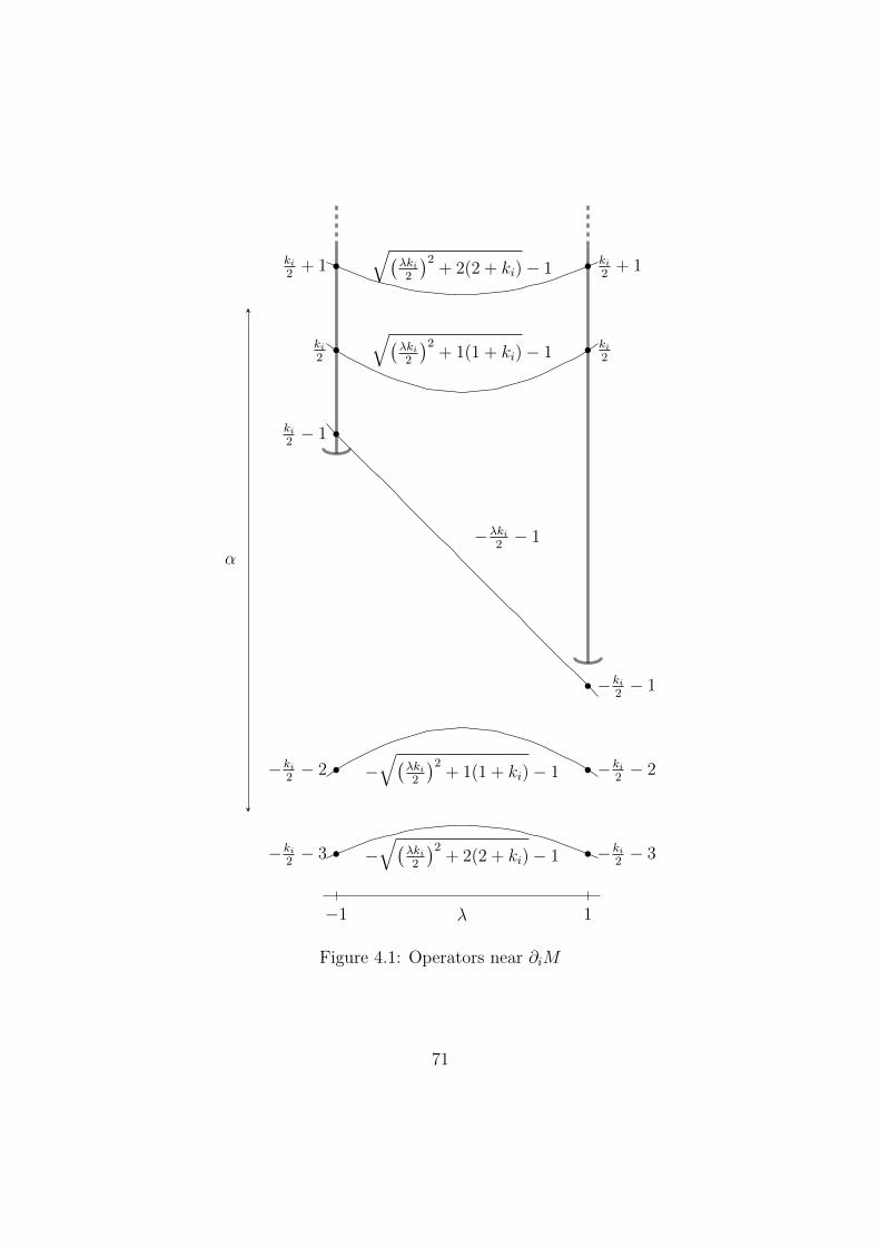
−√(
λki2
)2+ 2(2 + ki)− 1
−√(
λki2
)2+ 1(1 + ki)− 1
−λki2− 1
√(λki2
)2+ 1(1 + ki)− 1
√(λki2
)2+ 2(2 + ki)− 1
−ki2− 3
−ki2− 2
ki2− 1
ki2
ki2
+ 1
−ki2− 3
−ki2− 2
−ki2− 1
ki2
ki2
+ 1
λ−1 1
α
Figure 4.1: Operators near ∂iM
71

−√(
λk2
)2+ 2(2 + k)− 1
−√(
λk2
)2+ 1(1 + k)− 1
−λk2− 1
√(λk2
)2+ 1(1 + k)− 1
√(λk2
)2+ 2(2 + k)− 1
−k2− 3
−k2− 2
k2− 1
k2
k2
+ 1
−k2− 3
−k2− 2
−k2− 1
k2
k2
+ 1
λ−1 1
α
Figure 4.2: Operators near ∂∞M
72

Bibliography
[ADHM78] Michael Atiyah, Vladamir Drinfeld, Nigel Hitchin, and Yuri Manin.Construction of instantons. Physics Letters A, 65(3):185–187, 1978. 1
[Agm82] Shmuel Agmon. Lectures on Exponential Decay of Solutions of Second-Order Elliptic Equations: Bounds on Eigenfunctions of N-Body Sch-rodinger Operations. (MN-29). Princeton University Press, 1982. 37
[AH88] Michael Atiyah and Nigel Hitchin. The Geometry and Dynamics ofMagnetic Monopoles. Princeton University Press, 1988. 24, 25
[Bal06] Werner Ballmann. Lectures on Kahler manifolds, volume 2. EuropeanMathematical Society, 2006. 14
[Cal78] Constantine Callias. Axial anomalies and index theorems on openspaces. Communications in Mathematical Physics, 62(3):213–234,1978. 37
[Dir31] Paul Dirac. Quantised singularities in the electromagnetic field. Pro-ceedings of the Royal Society of London. Series A, Containing Papersof a Mathematical and Physical Character, 133(821):60–72, 1931. 1
[DK90] Simon Donaldson and Peter Kronheimer. The Geometry of Four-manifolds. Oxford mathematical monographs. Clarendon Press, 1990.34
[Don84] Simon Donaldson. Nahm’s equations and the classification of mono-poles. Communications in Mathematical Physics, 96(3):387–407, 1984.34
[Fri00] Thomas Friedrich. Dirac Operators in Riemannian Geometry. Amer-ican Mathematical Society, 2000. 3, 12
[GH78] Phillip Griffiths and Joe Harris. Principles of Algebraic Geometry.Wiley, 1978. 14
73
[Hit74] Nigel Hitchin. Harmonic Spinors. Advances in Mathematics, 14(1):1– 55, 1974. 12
[Hit83] Nigel Hitchin. On the construction of monopoles. Communications inMathematical Physics, 89(2):145–190, 1983. 1, 33, 34
[Hit92] Nigel Hitchin. Hyperkahler manifolds. Seminaire Bourbaki, 34:137–166, 1992. 17, 32
[Jar04] Marcos Jardim. A survey on Nahm transform. Journal of Geometryand Physics, 52(3):313–327, 2004. 34
[JT80] Arthur Jaffe and Clifford Taubes. Vortices and monopoles: structureof static gauge theories. 1980. 19, 43
[Kuw82] Ruishi Kuwabara. On spectra of the laplacian on vector bundles.Journal of mathematics, Tokushima University, 16:1–23, 1982. 63
[LM89] H. Blaine Lawson and Marie-Louise Michelsohn. Spin Geometry. Prin-ceton University Press, 1989. 3
[LMO85] Robert Lockhart and Robert Mc Owen. Elliptic differential operatorson noncompact manifolds. Annali della Scuola Normale Superiore diPisa-Classe di Scienze, 12(3):409–447, 1985. 62
[Mel93] Richard Melrose. The Atiyah-Patodi-Singer Index Theorem. ResearchNotes in Mathematics. CRC Press, 1993. 58, 62
[Mel95] Richard Melrose. Geometric scattering theory, volume 1. CambridgeUniversity Press, 1995. 67, 68
[Mel08] Richard Melrose. An Introduction to Microlocal Analysis. 2008. 67
[Nah83] Wener Nahm. All self-dual multimonopoles for arbitrary gauge groups.In Structural elements in particle physics and statistical mechanics,pages 301–310. Springer, 1983. 1, 33
[Nak93] Hiraku Nakajima. Monopoles and Nahm’s equations. Lecture Notesin Pure and Applied Mathematics, pages 193–193, 1993. 2, 33, 34, 41,57
[Sin00] Michael Singer. Dirac Operators Coupled to Dirac Monopoles. Un-published, 2000. 62
[Tau83] Clifford Taubes. Stability in yang-mills theories. Communications inMathematical Physics, 91(2):235–263, Jun 1983. 21, 24, 26
74
[TM79] P. Tataru-Mihai. On the prasad-sommerfield dyon (monopole) solu-tion. Letters in Mathematical Physics, 3(5):437–444, Sep 1979. 20
[WGP80] Raymond O’Neil Wells and Oscar Garcıa-Prada. Differential analysison complex manifolds, volume 21980. Springer Berlin, Heidelberg, NewYork, 1980. 14
75