Monograph - Chapter XX - SOA Financial Reporting Section ...

XX Market Value of Insurance Liabilities: Reconciling the

Actuarial Appraisal and Option Pricing Methods

Luke N. Girard

Abstract With Statement of Financial Accounting Standards

115 (FASB 1993), insurers are now in the awkward situation that almost half of the balance sheet is marked to market. This has created a material inconsistency with the way liabilities are reported, thus diminishing the usefulness of financial reporting to shareholders and potential new investors. Discussion has emerged in the industry about the process of market valuing liabilities. The American Academy of Actuaries has formed a "Fair Valuation of Liabilities" task force to compare and review various alternative methodologies. During 1995 the Society of Actuaries and New York University jointly sponsored a conference on "Fair Value of Insur- ance Liabilities." Motivated by the conference, this paper attempts to bridge the g~ip between option pricing and actuarial appraisal methodologies. The author suggests we refocus attention toward the assumption-set- ring process, which is the key driver of a fair valuation. In this regard, this paper attempts to advance practice and methodology with respect to life insurance company valuation.

1. Introduction With Statement of Financial Accounting Standards

115 (FASB 1993), insurers are now in the awkward situation that almost half of the balance sheet is marked to market. This has created a material inconsistency with the way liabilities are reported, thus diminishing the usefulness of financial reporting to shareholders and potential new investors. Also, the risk management tool of value-at-risk measurement, which has been the domain of our large banking institutions, is beginning to filter into the insurance industry. The key underpin- ning of such a process is an appropriate market valuation process. This paper endeavors to advance practice and methodology in all these areas.

Discussion has emerged in the industry about the market valuation of liabilities. The American Academy of Actuaries has formed a "Fair Valuation of Liabili- ties" task force to compare and review various alterna- five methodologies. The task force produced a discussion paper, which was presented at the "Fair Value of Liabilities" conference sponsored by the Soci- ety of Actuaries and the Salomon Center at the NYU Stern School of business. Also, several other papers were presented at the conference on this subject and are referred to in this paper (see Doll et al. 1998).

XX. Market Value of lnsurance Liabilities: Reconciling the Actuarial Appraisa.l and Option Pricing Methods 261

In their paper the task force cataloged seven methods for calculating fair values. Two of these methods, the actuarial appraisal method (AAM) and the option pricing method (OPM), are the subject of this paper. Under the AAM, the valuation is done by deducting from the market value of the assets the present value of free cash flow discounted at the cost of capital. This contrasts with the OPM, in which the valuation is conducted similarly to the valuation of corporate debt by discounting the liability cash flows directly. Section 2 is a general overview of the AAM with an explanation of how it compares to the OPM. The reader can omit this section if he or she is already familiar with these two methods. This paper attempts to bridge the gap between option pricing and actuarial appraisal methodologies.

The AAM is the method used by actuaries when valuing insurance companies and blocks of insurance business. Price discovery occurs when these blocks trade in the reinsurance marketplace. As far as investors in insurance businesses are concerned, this is the relevant marketplace. Valuations are done by using the AAM, and in most cases assumptions are set in part based on the capital markets and in part based on actuarial judg- ments as to what future experience will be. Typically the assumption is not made that the underlying insurance policies are tradable as securities. In contrast, the OPM is used to value the asset side of the insurance company balance sheet with assumptions derived from the capital markets and that these instruments are tradable as investments. This situation presents the possibil- ity that assets and liabilities may not be valued consistently, with one side valued with one set of assumptions while the other side is valued with a different set of assumptions. Thus, the true value of the company's equity may be obscured by inconsistent assumptions.

A first step in ensuring consistent assumptions is to reconcile these seemingly different methodologies. We accomplish this by showing that discounting free cash flow is actually the same as discounting the actual asset and liability cash flow. Section 3 provides an intuitive explanation why this must be the case. Section 4 shows mathematically that discounted distributable earnings (DDE), calculated using the actuarial appraisal method, can be decomposed into components comprising of required surplus (RS), market value of assets (MVA), market value of liabilities (MVL), tax value of assets (TVA), and tax value of liabilities (TVL), as shown in this relation:

DDE = RS + (1- T)(MVA - MVL) + T(TVA - TVL).

Moreover, the RS, MVA, and MVL components can be valued separately using the option pricing method. In Section 5, this result is extended from the static world to the world of uncertainty.

If these two seemingly different methods are the same, why are practitioners getting different results? The only possible explanation is that the assumptions are not being applied consistently between the two methods. Section 6 reviews the implications for selecting the interest rate scenarios and the cost of capital. In the application of the AAM without taxes, it is shown that if we use risk-neutral valuation and a leverage- adjusted cost of capital, then the valuation is identical to discounting liability cash flow directly at the risk-free interest rate plus a credit spread. With taxes, an allow- ance needs to be made in the discounting rate for tax COSTS.

To illustrate the concepts presented in this paper, Section 8 provides a numerical example for a guaran- teed interest contract (GIC). Section 9 summarizes the paper's conclusions.

2. An Overview of Actuarial Appraisal Methods

In any discussion of valuation of an insurance enterprise, a good starting place is the actuarial appraisal process, where standards are well defined and there exists published literature on the subject. The Actuarial Standard of Practice no. 19---Actuarial Appraisals was adopted by the Actuarial Standards Board in 1991. This standard provides useful insight concerning current methodology and the responsibilities actuaries have concerning disclosures and communications to clients.

The traditional approach to actuarial appraisals is to consider the target company or block of business as made up of three components for which values are determined separately. The appraised value is then the sum of these three elements (see Guinn, Baird, and Weinhoff 1991, Thompson, Millar, and Riggieri 1992, and Turner 1978).

Adjusted Net Worth Adjusted net worth is the value resulting from the

statutory surplus of the company. "Adjusted" is taken to mean that it is not appropriate to simply take the reported statutory statement value of surplus as this value. Reported surplus needs to be increased or decreased by other amounts judged to be in the nature

262 Financial Reporting Section Monograph

of such funds. Examples of such adjustments include the asset valuation reserve (AVR), deficiency reserves, cost of collection, and nonadmitted assets. The value of

surplus is represented by the assets of the company allocated to surplus. Since assets are valued at amortized cost on the balance sheet, adjusting these assets to market is viewed as appropriate.

Value of ln-Force Business Value of in-force business is the present value of

future after-tax statutory earnings on the existing in force as of the valuation date. At one point there were questions as to whether the appropriate accounting basis should be GAAP or some other basis. Now it is fairly well established that statutory accounting is the correct basis since this defines "free cash flow" available for distribution to shareholders as dividends. There were also questions as to whether the projected• earnings should be pretax or after-tax. It is clear now that it is inappropriate to do a valuation on the basis of discounting pretax earnings.

An open question is whether the adjusted net worth component should be reduced by the risk-based capital needs of the block of business being valued. The investment earnings along with the repayment of this capital would then be included as part of free cash flow. The rationale for this is that an insurer cannot distribute to shareholders all of its surplus since such an insuranc~

• enterprise needs to maintain a reasonable cushion to offset plausible future adverse deviations in experience. Rating agencies require minimum surplus levels for companies to maintain their ratings, and regulators require companies to maintain adequate surplus levels. Therefore, the emerging current practice is to incorpo- rate risk-based capital into the appraisal process, or, if it is not done, that this is adequately disclosed (see Becker 1991 and ASOP no. 19).

Considerations in setting the discount rate or "hurdle rate" include the following: • First, the riskiness of the stream of future cash flow.

In theory, the discount rate can vary significantly with the perceived riskiness of the transaction.

• Second, the return desired by the buyer or seller based on investment opportunities available else- where for similar risks.

• Third, the buyer's or seller's cost of capital.

Value of New Business Value of new business is the discounted present

value of the earnings on new business. In many instances, because of the uncertainty of new sales and the profitability of such sales, this component of the valuation may be given a zero or even a negative value.

Because of the inherent riskiness of this business, the • discount rate could be significantly higher than for the

valuation of the in-force block. If different dis-count rates are used for new and in-force business, the appraisal may include an "expected aggregate return" for the combined block.

Turner (1978) suggests using a single discount rate for both in-force and new business. Pricing for the extra risk of new business would be accomplished by using more conservative assumptions than "best estimate" assurhp- tions. This approach has similarities to the risk-neutral valuation process used in option pricing methods.

The AAM versus the OPM The AAM approach to valuation differs significantly

from the OPM. The main differences between the OPM and the AAM are the following: ~ • Under the OPM, the discounted cash flow is the

actual asset or liability cash flow, while under the AAM, the cash flow is the free cash flow as defined by statutory accounting and required risk-based capital.

• For the OPM, the discount rate is the risk-free rate plus a spread. 2 The spread is determined such that the present value reproduces observed market pricing for such insurance liabilities or similar financial instruments. For the AAM, the discount rate is a risk- adjusted cost of capital rate.

• Under the OPM, pricing for risk is accomplished by using risk-adjusted scenarios. Under such scenarios, the "true" probability distribution is risk-adjusted or tweaked to reflect risk premiums priced into the market. Under the AAM, the general practice is to use the true probability distribution with risk pricing occurring via the discount rate. More often than not, uncertainty in assumptions is dealt with deterministi- cally. 3

• Underthe AAM, cost of capital is recognized explicitly through the cost of capital discount rate, and an explicit assumption is usually made concerning corporate income taxes. Under the OPM, these costs are recognized implicitly in the spread assumption that

XX. Market Value of lnsurance Liabilities: Reconciling the Actuarial Appraisal and Option Pricing Methods 263

is added to the risk-free rate. To argue that the OPM ignores cost of capital and taxes would be to say that the market does not consider such costs. If the market did not price for these costs, the supply of capital would quickly dry up, and these insurance products would cease to exist.

• Transaction costs arising due to investing and disinvest- ing and cost of carry from borrowing are often modeled explicitly with respect to the AAM. For the OPM, these costs are implied in the spread assumption. Indeed, the spread assumption with the OPM is play-

ing multiple duty. Furthermore, the implicit nature of the assumptions process make it rather difficult to determine to what extent these costs are provided for.

The AAM and OPM have many similarities, and in particular the AAM is general enough to accommodate option pricing methodology. For example, behavioral assumptions such as policy lapsation, mortgage prepay- ments, and crediting strategies are usually modeled dynamically for both approaches.

AAM Assumptions The setting of assumptions is perhaps the most criti-

cal aspect of the AAM and is quite comprehensive. Examples of assumptions that are made include such items as mortality, morbidity, operating expenses, taxes, interest rate scenarios, reinvestment and disinvestment strategies, investment expenses, default experience, inflation, reinsurance costs, policy lapsation, capital requirements, reserve basis, policy loans, crediting and repricing strategies, and new business.

Substantial judgment is normally involved. Consid- erations in setting assumptions include the following: • Availability of relevant experience, whether at the

company or industry level • Current business and economic trends in experience • Company operating strategies • Competitive environment • Sensitivity testing.

Generally assumptions are not "market implied" since usually they are based on experience trends and judgment. For example, mortality assumptions would be based on actual experience modified appropriately for future trends, and not on how the market views "mortality risk" from a risk-pricing standpoint. Excep- tions to this would be certain investment assumptions, prices charged by suppliers, and the risk premium in the discount rate. It may be intuitively appealing to use

"market-implied" assumptions; however, most insurance risks do not trade actively, and in the end the practical answer is to rely on an expert's opinion. Nevertheless, it would seem to make sense for such an expert to consider, in concept, how the market prices risk by observing the market's pricing of risks that do trade.

Considerable disagreement can exist between actuaries representing sellers and buyers. The general rule that the buyer's appraisal is approximately 40% of that produced by the seller is not too far off the mark (see Guinn, Baird, and Weinhoff 1991).

3. The Components of DDE: Intuitive Reasoning

As mentioned in Section 2, the AAM dissects the appraisal process into three pieces. The value of free surplus is adjusted statutory surplus minus the amount of risk-based capital needed to support existing in-force business. Since free surplus is immediately distributable, no discounting of this amount is necessary, or the discounted value is simply the amount of free surplus. The second component is the present value of distributable earnings from the in-force business. The third component is the present value of distributable earnings from new business, also known as franchise value. The following discussion will focus on the second component of the AAM, the value of in-force business.

For in-force business, the key analytical concept of the AAM is represented by the formula for discounting free cash flow or discounted distributable earnings (DDE). This formulation is the generally accepted approach to valuation within the actuarial community.

For an insurance company, this approach can be used to value blocks of in-force business acquired directly or via reinsurance transactions:

D O E = ]~ B E t (1 + k)-',

where DE, is distributable earnings and k is the cost of capital.

In accordance with the AAM, the basis for distributable earnings is after-tax statutory income reduced by the increase in risk-based capital requkements:

DE, = I, - ARS,_ t, (3.1)

where I, is after-tax statutory income and ARS,_z is the change in required surplus. 4


It is possible to reformulate DDE into three parts:

DDE = RS + (1 - T)(MVA - MVL) + T(TVA - TVL). (3.2)

Here T is the tax rate, MVA is the market value of assets, TVA is tax value of assets, and TVL is tax value of liabilities. MVL is the market value of a block of insurance liabilities as they would trade between insurers in the reinsurance market; it is not the market value of the insurance policies in a market where these policies are freely traded, that is, where policy-holders can sell their policies to investors or to other policyholders. Thus, this formulation does not imply the existence of an active primary and secondary market for insurance policies. However, it does imply the existence of an active secondary market for blocks of insurance liabilities in the reinsurance market.

It is important to note that the above equality holds only if we make the same assumptions in both Equa- tions (3.1) and (3.2). For example, if we assume the cost of capital is 12% in Equation (3.1) and then implicitly assume 10% in Equation (3.2), we will not obtain the same result. This may be stating the obvious. However, detractors will do this, perhaps unwittingly, and then declare that the decomposition cannot hold.

An important point needs to be emphasized with respect to notation. The terms. MVA and MVL are used to mean market values. This presumes that the assumptions on which their valuation is based on are derived from the marketplace. The equation still holds if we do not use such assumptions, but MVA and MVL would no longer be market values, and DDE would not be based on market assumptions. In such an event, we may want to use different terminology such as present value, appraised value, or economic value.

The last expression, comprising TVA and TVL, is an adjustment for the timing of tax payments when the tax basis for assets and liabilities is different from the statutory basis. If TVA and TVL are equal to statutory values of assets and liabilities, respectively, then TVA becomes equal to TVL, and no adjustment for timing is required. 5

Below is the intuitive reasoning underlying the decomposition. A mathematical proof is provided in the Appendix.

Required Surplus The first component, required surplus (RS), repre-

sents the market value of a portfolio of assets that has a

statutory book value equal to the surplus requirement. 6 In a direct new business or reinsurance transaction, this component can be viewed as the capital contributed by the shareholders of the direct insurer or reinsurer to fund risk-based capital requirements.

As mentioned earlier, DDE as shown here is the value of in-force business and includes the associated required surplus, but not the value of free surplus, which is immediately distributable.

Market Value of Assets The portfolio of assets that make up MVA is a portfo-

lio that has a statutory book value equal to the statutory book value of the policy liabilities. MVA excludes surplus assets since these are included in the first part of the DDE decomposition. The decision to exclude them from MVA is arbitrary. If they were to be included in MVA, the RS term would disappear but at the expense of complicating the analysis that follows. While this con- vention simplifies the analysis, it is also the basis on which many reinsurance transactions are settled. The philosophy is consistent with the situation in which surplus assets are managed in a separate portfolio and the product portfolio's assets are maintained such that the statutory book value of assets is equal to the statutory book value of policy liabilities.

It should be noted that MVA also includes the value of future assets purchased with product cash flow, including premium income on in-force policies, and reinvestment of cash flow from existing in-force assets. If the scenarios used in the appraisal process are arbitrage-free, then the market value of future investment and reinvestment is zero. 7 On the other hand, if the scenarios used are not arbitrage-free, then the value of future investment may not be zero. Often it is the practice not to require arbitrage-free scenarios, and if this is the case, future investment will have a nonzero valuation. In this situation, the use of the term market value, or even fair value, is inappropriate.

Market Value of Liabilities For the purpose of understanding the relationship

between DDE, MVA, and MVL, the liability cash flows that form the basis for MVL are defined comprehensively to parallel the AAM. Cash flows include after-tax required profit as well as benefits, premiums, net change in policy loans, policy loan interest, commissions,

XX. Market Value of lnsurance Liabilities: Reconciling the Actuarial Appraisal and Option Pricing Methods " 265

operating expenses, policyholder dividends, re-insurance premiums, reinsurance claims, premium taxes, and income taxes. MVL can be thought of as the cost of purchasing a benchmark portfolio of securities in which the benchmark, net of investment expenses and defaults, replicates the cash flows. Moreover, if all the liability assumptions materialize, including assumptions made concerning investment expenses, defaults, and payments.to shareholders, the benchmark securities will produce sufficient cash flow to exactly satisfy the liabilities.

Rather than using the benchmark approach described above, MVL could be calculated by discounting the cash flow using the government yield curve plus an appropriate spread. If this spread is the option-adjusted spread (OAS) of the benchmark portfolio, net of investment expenses and defaults, as described above, then such a calculation will yield a value equal to the cost of purchasing the benchmark portfolio mentioned above. If such a benchmark is not readily available, a guide for this spread is the OAS of an existing portfolio when such a portfolio is a good proxy for this replicating strategy. The portfolio OAS can be estimated by calculating the duration- and market-value-weighted OAS of the individual securities in the portfolio since this is a good approximation of the OAS of the aggregate portfolio. Note that the term structure of spreads, like the government yield curve, is not flat and is implicit in the market's pricing of the benchmark. Policy premiums are considered here to be negative liability cash flows, and it is also valid to consider these as positive asset cash flows. This distinction is irrelevant to the DDE calculation using the AAM since the discounting of assets and liabilities is implicitly done with the same yield cu / ' v e .

Alternatively, liability cash flow could be defined less comprehensively so as not to include after-tax required profit and income taxes on such profits, s In such an event, the discount rates or spreads would need to be adjusted downward in order to provide for these costs.

There is an interesting recursive relationship between the liabilities and the benchmark investment portfolio described above. Valuation of liabilities includes assumptions about defaults, cost of capital, and investment expenses. This means that we cannot determine the cost of the liabilities independently of the investment strategy. Furthermore, if an asset class has a high OAS relative to the assumptions made about defaults, cost of capital, and investment expenses, then

the more the company invests in such an asset class the higher the appraised value will be. This is an inauspi- cious result with respect to the application of the AAM. The source of this problem appears to arise from the failure to adequately adjust the risk premium inherent in the cost of capital rate that is used to discount free cash flow. A discussion of this important issue is included in Section 6.

It is also important to distinguish between two very different markets for insurance liabilities. One of these markets is the market where insurers issue policies to policyholders and where insurers compete with each other for market share. Also, in this market insurers will trade blocks of liabilities with other insurers in the reinsurance and the merger and acquisition marketplace. MVL, as described above, is the value of these liabilities as they trade in this marketplace. This is the market that investors and managers of insurance companies are most concerned with and where the AAM is generally used.

The second market is the market where the policies themselves trade between policyholders and investors. Examples of these markets are the secondary GIC market and viatical settlements. This market is more of a "garage sale" and is somewhat irrelevant, as far as investors in insurance companies are concerned. Gener- ally, insurance policies are not tradable securities and are not designed to be such. Policies are designed to meet personal need and are, in a sense, personal property. Moreover, they have a financial value, and if they lose their appeal to the owners because of changing personal situations, they can become tradable securities, for a price. The term MVL, described above, is not meant to be the value of such policies in such a market. Valuation in these two markets is different, even in fric- tionless perfect markets.

Embedded Value The term (1 - T)(MVA - MVL) can be viewed as

"embedded value" (EV) since it is a measure of what a shareholder would pay on an after-tax basis for a block of business to exactly earn the cost of capital. In a reinsurance transaction, if EV exceeds the after-tax ceding commission, the amount paid by the reinsurer to the ceding company, then EV less the ceding commission and less any acquisition expense is the "economic value created" by the transaction on the reinsurer's books. For a direct insurer writing new business, the amount "paid" by the insurer for the business is the


difference between the initial statutory reserve and the premium collected, net of acquisition expenses and tax credits. This is so because regulation requires that assets equal statutory reserves. Usually. the assets provided by the policyholder are not sufficient to fund the entire reserve, and additional assets need to be contdb: uted by the insurer to fund this difference. As with the reinsurance transaction, the "economic value created" is EV less this amount "paid" by the insurer for the business. In fact, for value-driven organizations, this may be the measure of sales performance as opposed to raw production volumes.

Required Profit As mentioned above, the definition of liabilities

includes a provision for profit, which can be intuitively viewed as an outflow payment amount to shareholders. Here this outflow is termed the required profit (RP):

+ (k - i , ) ( M V A ; _ I - MVLt_I )

+ I-~ T(TVAt-I'- TVL'-I)" (3.3)

Here k is the costof capital, j is the interest rate earning on required surplus, and i is the interest rate earning on the portfolio assets. The cost of capitalk is risk-adjusted to reflect the risk inherent in the stream of free cash flow. RP, RS, MVA, MVL, TVA, and TVL are allowed to take on different values in future time periods. For simplicity, it is assumed that.' the cost of capital .and surplus interest rates do not vary with time? This expression is a pretax margin; that is, it includes a provision for taxes that are paid. To obtain the after-tax required profit, simply multiply both sides by (I - T):

(I - T)RP t = [k - (I - T)j]RSt_ l

+ (1 L T) (k - i t ) ( M V A t _ I - MVLt_I) + kT(TVAt_ ! - T V L J .

This expression represents the payments to shareholders, which, when added to after-tax interest on invested capital, equal the cost of capital required by shareholders. Here invested capital is taken to mean the investment by shareholders initially and at future time

periods. The total shareholder investment is

D D E t = R S t + (1 - T) (MVA t - MVL, ) + T(TVA, - TVLt).

In the fast term of Equation (3.3) k/(1 - T) is the pretax required profit on invested capital needed to fund required surplus. The cost of capital is reduced by surplus interest since the product only needs to make up the difference between the required rate and what surplus can generate on its own. We do not divide j by (1 - T) sincej is already pretax.

The second term of Equation (3.3) recognizes the cost of capital for the embedded value in the business, which includes both the-amount "paid" for the business and the "value created." It can be rewritten as

(k - it)(MVA,_ ~ - MVLt_t)

k - i t = 1 - T (1 - T ) (~ .A . ._ t - MVLt_I).

Here (1 - T)(MVAt_, - MVLt_ 0 is the embedded value and [(k - it)~(1 - T)] is the pretax required profit on investment capital needed to fund the embedded value. The cost of capital k is divided by (1 - T) in order to obtain the pretax cost of capital. The interest rate i is already pretax and should not be divided by (1 - T); then why is it divided by (1 - T)? It isn't! There is another factor equal to TI(1 - T) due to the tax benefit from the embedded value not being taxed currently and deferred via the taxreserving mechanics. This tax benefit effectively offsets the cost of capital. Therefore, the factor for i is [1 + TI(1 - T)] = 1/(1 - T). Finally, the interest rate is i, not j, since the embedded value is invested in the product portfolio.

If the tax basis for either assets or liabilities is different from the statutory basis (for example, market discount, real estate depreciation, DAC taxes, the applicable federal interest rate, IMR), then there may be additional payments to or from the government that require or generate capital. The last term comprising T(TVA - TVL) is this measure of the capital used or generated. The after-tax required profit for this capital is k, and we need to divide by (1 - T) to obtain the pretax requirement. We don't subtract i or j because the government does not pay the company any interest on this timing difference, and the product needs to make up the entire cost of capital on a pretax basis. Indeed, this is expensive capital, indicating there may be value in tax planning.

XX. Marke t Value o f Insurance Liabilities: Reconci l ing the Actuarial Appraisal and Option Pricing &1ethods 267

The Three Parts of the AAM Revisited The above discussion focuses on the second compo-

nent of the AAM, the present value of distributable earnings from in-force business. While this was done for simplicity, these concepts can be easily extended to include the other two components involving free surplus and new business.

To see this for free surplus, we can think of the value of free surplus as the sum of the three components of required surplus, embedded value, and the tax basis adjustment (TBA). For free surplus, both the E V and the

TBA are equal to zero since there are no product assets and liabilities. If we redefine RS to be the assets supporting free surplus at time equal zero, that is, the valuation date, then this becomes the only nonzero term of the decomposition. This indeed is the value of free surplus since it is immediately distributable.

For new business, if our valuation process is arbitrage-free, the first term involving RS is zero. This is so because the value of purchasing future assets at market prices is zero. If the valuation process is not arbitrage- free, then the RS term would be nonzero. The tax basis adjustment is zero because at the valuation date there are no product assets or liabilities. The E V is slightly more complicated. As with RS, the MVA term is zero because the value of purchasing future assets at market prices is zero. This leaves just the term involving MVL, or more specifically

- (1 - T)MVL..

Generally this term will not be zero and could be either positive or negative. This is true whether or not we use an arbitrage-free valuation process. If we use an arbitrage-free valuation process, MVL would be zero only if the insurer priced its products fairly in relation to the capital markets and we ignored taxes. If the business is profitable, then the value of future premiums should exceed the value of future benefits and expenses. This will make MVL negative, and the preceding negative sign will convert the negative MVL to a positive number as it should be for profitable business. If the business is not profitable, MVL will be positive, and the preceding negative sign will convert the positive MVL term to a negative number as it should be for unprofit- able business. The factor (1 - T) isto reflect that new business profits will be subject to taxation; that is, MVL is pretax.

Fair Value of Liabilities: Deductive Methodology

The assets were arbitrarily split between those supporting the required surplus requirement and those supporting product liabilities. This was done for a number of reasons: consistency with the way many re-insurance transactions are settled, consistency with the historical actuarial appraisal process of dissecting the valuation between surplus and in-force business (Turner 1978), and to highlight how risk-based capital affects leverage and hence valuation.

We could have defined MVA to include both product assets and surplus assets. If we define MVA* to be the market value of all the assets of the finn, then

MVA * = R S + MVA.

Similarly, if we define TVA* to be the tax value of all the assets of the firm, then

TVA * = RS + TVA.

Equation (3.2) can be rewritten as

D D E = (RS + MVA - M V L )

- T[(RS + MVA - RS - TVA) - (MVL - TVL)].

If we make substitutions for MVA* and TVA*, we obtain

D D E = (MVA* - M V L ) - T[(MVA* - TVA*)

- ( M V L - T V L ) ] .

The last equation shows that D D E is simply the difference between the market value of assets and the market value of liabilities minus a "deferred tax liability" adjustment. This presentation corresponds with GAAP; however, to accomplish this, M V L has been explicitly defined.

We can" also rearrange the DDE decomposition formula as follows:

M V L = ( M V A * - D D E )

- T[(MVA* - TVA*) - (MVL - TVL)]. (3.4)

This shows that, if we know the market value of the assets of the firm and the appraisal value, then the market value of liabilities can be deduced. If we ignore the


last term involving taxes, we get the same expression as Doll et al. (1998): ~°

MVL = MVA* - DDE. (3.5)

If the market value of assets and liabilities are equal to their tax values, then the expression.in Equation (3.5) produces the same result as Equation (3.4). This is not likely to be the case because of special tax regulations for valuing assets and liabilities. Even if they are the same at policy issue, after policy issue they will diverge when the market values change because of market factors.

4. Equivalence of AAM and OPM

DD E Decomposition Proposition Discounted distributable earnings, calculated using

the AAM, can be decomposed into three components of required surplus, embedded value, and a tax basis adjustment. The embedded value is the tax-adjusted difference of the market value of product assets and liabilities. The last term is the tax basis adjustment, and it reflects differences ~n basis between tax and statutory accounting. DDE can be reformulated as follows:

DDE t = RS, + (1 "- T)(MVAt- MVL,)

+ T(TVA t - TVL,). (4.1)

Note that the proposition depends only on the definitions that follow. No assumptions are made regarding perfect markets or that liabilities can be traded between investors and policyholders.

Definitions t = Time period, where t = 0 to N. At the valuation

date, t = 0. The period havingthe last free cash flow is designated as period N.

RS, = Required surplus. By assumption, unrealized gains and losses are ignored; hence RSt is also the statutory, market, and tax value of assets supporting the risk-based capital requirement. H

k = Cost of capital, and it is assumed not to vary over time and k ~ -1.

j = Interest rate earned on required surplus assets, net of investment expenses and investment defaults. It is assumed not to vary over time. ~2

SVA,

i,= Risk-adjusted discount rate for the product • assets. The interest rates i, are forward rates.

Product assets are those assets designated to support the liabilities such that the statutory value of assets equals the statutory value of liabilities. These assets along with the assets supporting required surplus are the total of all the assets needed to support the liabilities under the regulatory environment. These interest rates are derived from the market's pricing of assets such that when we discount the asset cash flow we get. the observed market value of the assets. The asset cash flow is net of expected default costs and investment expenses, and-therefore the interest rate is also net of expected default costs and investment expenses.

T = Corporate income tax rate. By assumption, capital gains and losses and ordinary income are combined for taxable income purposes and are taxed at a single rate. Tax losses are assumed to be utilized when they are incurred; that is, the company is not in an operating loss carryover position. It is possible to relax these assumptions at the cost of introducing additional com- plexity in the tax calculation.

11, = Investment income on product assets, assuming statutory accounting. It includes coupon income, accrual of discount and premium, and capital gains and losses. It is reduced for investment expenses, provisions for investment defaul'ts, investment transaction costs, and any negative or positive carry, ff borrowing is required.

A t - - All asset cash flows with respect to product assets. It includes coupon income, maturities, proceeds from sales, and cash disbursements to fund future reinvestment. Note that product assets include reinvestment. Reinvestment could be excluded if the in-force assets are exactly cash matched with in-force liabilities. This is seldom the case in practice, and therefore it must be considered here.

E, = Expenses include operating expenses, commissions, and premium taxes.

L, = Net policyholder cash flows. It includes benefits, premiums, policy loans, 13 reinsurance premiums, re-insurance claims, and any fees charged. and TVA, = Statutory and tax value of product assets, respectively. It excludes policy loans.


S V L t and TVL, = Statutory and tax value of liabilities, respectively. It includes the IMR and is reduced by policy loans.

Tax basis adjustment:

T B A t = T ( T V A t - TVL, ) . (D 1)

II, can be written as

l i t = A , + ASVA,_ I . (D2)

This relation comes from the double-entry accounting principle that credits must equal debits. If we record income (II~), it is a credit, and the offsetting debit is either to cash (A,) or to invested assets (z3SVAt_I). For a bond purchased at par, A, would reduce to the coupon payment and ~SSVA,_~ would be zero until the maturity event. At maturity, two entries would be made. The first would be to record the coupon income. The second would be to record the receipt of maturity proceeds. Thus, A t would include maturity proceeds (debit to cash), but this would be offset by an exact equal but negative amount of ASVA,_~ (credit to invested assets), ff a bond is purchased at a premium or discount, ~ V A t _ ~ would reflect the amortization. If an asset is purchased in a future period, the disbursement would be included in A, as a negative amount. This disbursement would be offset by an accounting entry to ASVA,_v ~4

Net Income is defined as

It = [II t + j (RS ,_ , ) - L , - z ~ V L , _ , - E,](1 - T)

- ATBAt_ v (D3)

This presentation of statutory net income into these components differs slightly from the usual analysis. Here investment income on product and surplus assets are shown separately) 5 To see this, start with the expression for investment income for product assets:

l i t = A t + ASVA,_ v

Similarly, the expression for taxable investment income is

TI1 t = A t + ATVA,_ v

Subtracting the first equation from the second, taxable investment income can be expressed as

TI1 t = II, + (ATVA,_, - ASVAt_I) .

Net income is pretax net income minus taxes:

1, = [111 + j (RS ,_ , ) - L , - z~VL,_~ Et]

- T [ T I I t + j (RS t_ ,) - L t - ATVLt_ 1 - E,].

Substituting the expression for Ti l t , we get

I, = [11, + j (gS t_ l ) - Z , - ASVLt_ t E,]

- T[TII , + (ATVA,_ I - z~VA,_I )

+ f iRSt_ l ) - L t - ATVLt_ I - Et].

Rearranging terms,

I t = (1 - T)[II , + j (RS t_ l ) - L , - ASVLt_ , - E,]

- T[(ATVA,_ I - ATVL~_I)

- (ASVAt_ l - ASVL,_O].

In a free cash flow model, S V A t = S V L t, since all excess cash flows are distributed; therefore net income simplifies to

I, = [11, + j(RSt_~) - L , - ASVL,_~ - E,](1 - T) - ATBA,_, .

(If this is not clear, see Appendix A for a more complete explanation.)

Distributable earnings are defined as

D E , = I, - z~S,_~, (D4)

and discounted distributable earnings as

D D E , + D E , and D D E N = 0. (D5) DDE~_I = 1 + k

This is the backward recursive version of the DDE equation D D E = Z, D E t ( 1 + k)-'.

Similarly, market value of assets is defined as ~6

M V A t + Ar MVA'- I = 1 + it and M V A N = 0, (D6)

and market value of liabilities as

M V L , ~ = M V L , + L, + E, + R P , and MVL N = 0. (D7) - 1 + i t

The definition for MVL is similar to that for the OPM in that we are directly discounting the liability cash flows. However, there are two important differences. First, we have an additional cash flow RP. Second, we

270 F i n a n c i a l R e p o r t i n g Sec t ion M o n o g r a p h

are discounting at the same rates that we discount the assets in order to determine MVA.

Required profit is defined as

+ (k - it)(MVAt_ t - MVL,-~)

• + I ~ T T(TVA'-I - TVLt-I)" 0)8)

This definition is important since it enables the decomposition. If the tax treatment of the middle term, comprising the EV, appears to be counterintuitive, the reader is referred to Section 3 for an explanation behind the meaning of the required profit.

The proof of the proposition is based on simple algebra and uses an induction argument. As it is somewhat tedious, it is shown in Appendix A.

Corollary: Equivalence of AAM and OPM By definition, the market value of liabilities is

MVL, + L, + E, + RP, JI4VLt-I = 1 + i, .0)7)

The vector i, of interest discount rates is risk- adjusted, and thus it can be expressed as a vector o f ' risk-free interest rates r t plus a risk premium 0A,. Note that the superscript A means that OAt is derived from the market's pricing of assets and is net of expected default costs and investment expenses.

Equation (D7) can be rewritten

MVLt + Lt + E, + RP, . MVL,_ I = .. (4.2)

1 +rt+0~

To see the equivalence of the AAM With the OPM, we defne the "liability spread" (0z)a's

OL t = OAt RP, (4.3) MVLt_ i."

The ratio RP, IMVLt_~ can be viewed as the required profit margin that needs to be deducted from the expected investment return before it can be used to discount the liability and expense payments.

Equation (4.3) can be rewritten as

RP, = (MVLt_t)(OA , - 0L,). (4 .4)

Substituting (4.4) into (4.2), we get the following relation for MVL:

MVLt_t = MVL, + L, + E, (4.5) 1 + rr + OLr

Equation (4.5) is exactly the form used with the OPM. The quantity 0Lt plus the risk-free rate is the interest rate used to discount the future liability and expense payments..

The equivalence above is based on pure algebra; that is, the equivalence holds for any set of assumptions. An ~ important difference between the methods is how assumptions are developed in each case. Under the OPM, this spread is explicitly defined. For example, it may be defined as made up of two components, a liquidity premium and a premium for the default option that the insurer owns. Another difference is that, under the OPM, expenses may be ignored. These assumptions are appropriate if the insurance liability is viewed similarly to corporate debt that is freely traded, t7 Although it would evolve into a messy insolvency and the investors would be wiped out, the insurer does own an option of putting to policyholders the assets of the company. See Merfeld (!995) for an application to life insurance and Copeland and Weston (1992) and Merton (1992) for a discussion of corporate debt issuance. An argument can be made that this concept is implicit within the AAM if the cost of capital assumption is derived from the marketplace. After all, if the investor owns such an option when purchasing a block of insurance policies, then he or she should recognize such value by using a lower cost of capital rate than what would be the case if such option did not exist. Thus, if the cost of capital is derived from the marketplace, the AAM should implicitly value such option.

Under the AAM the assumptions that are established implicitly define this spread, that is, 0 L. This spread can be obtained from the spread derived from the assets, OA, and by deducting the required profit margin. Therefore, these assumptions depend on statutory accounting, taxes, risk-based capital, investment strategy, and the cost of capital. As the riskiness of the investment strategy increases, 04 increases. However, the required profit margin ratio of RP/MVL also increases if the cost of


capital increases with the riskiness of the investment strategy. Under the AAM it is not clear how these factors offset each other. A discussion of these assumptions is included in Section 6.

Many practitioners, in declaring that these methods are different, are not being diligent in ensuring that assumptions are being applied consistently between the two methods. Whether assumptions are derived implicitly or explicitly or whether each method uses different assumptions should not be sufficient cause for these two methods to be viewed differently. After all, within each method different methods exist for developing assumptions. If this was a sufficient argument to make the two methods different, then we would arrive at the absurd conclusion that each method would be different from itself. Thus, if we make exactly the same assumptions in applying each method, we will get exactly the game result. This makes the two methods equivalent, although the manner of arriving at the assumptions may differ depending on the application.

5. Uncertainty and Interest-Rate- Sensitive Cash Flow

The Static World to the Uncertain World The DDE decomposition equation is based on the

static case when cash flows are not interest-rate sensitive. When cash flows are interest-rate sensitive, the proof and equations are for one scenario path from the universe of all possible paths.

Becker (1991) discusses the concept of discounting free cash flows or distributable earnings in the world of uncertainty. Distributable earnings are projected similarly to the way it would be done in an actuarial appraisal. The interest rate scenarios would be generated stochastically, and they would form the underlying basis for the distributable earnings projections. ff we have a set of P arbitrage-free paths for the risk- free rate,

{ rp . , : l<p<P and I < tAN} ,

where p represents a path and t represents a future period, then the option-adjusted value is determined as follows: Step 1: Using the recursive relationship, DDEp.,_ I =

(DDEp., + DEp.,)I(1 + kp.,), calculate DDE for each forward time-step along each path. DDEp., stands for the pathwise DDE value for path p at the forward duration t, with DDEp., = 0. Furthermore, k is the cost of capital, and it is assumed to vary with state and time. 18

Step 2: To get the option-adjusted price, calculate the probability weighted average pathwise value at t = 0. The valuation formulas for the uncertain world are

shown in Table 1 along with their static world analog. The probability for each path is denoted by %. The decomposition holds for the static world and for each path in the uncertain world. Since they hold for each path, they must also hold for a probability weighting of all the paths. The proof of this is trivial. Note that the bars over the rates k, r, and 0 mean that the rates are written in the form of spot rates and not forward rates.

6. The Assumptions In Section 4, it was asserted that the OPM and the

AAM are equivalent. However, practitioners, in applying each method, are getting different results. If the methods are equivalent, then the only possible explanation is that practitioners are not being careful in reconciling their assumptions. There are many assumptions that are made that can cause the two methods to deviate from each other. Under the AAM often the objective is to value a block of insurance policies. Assumptions are usually based on experience studies and the actuary's judgment concerning the future out-look. Except for interest rates, assumptions are usually not based on the "market's view." This may be satisfactory if the objective of the valuation is to come up with some sort of internal management measure of economic value. How- ever, this practice could be problematic if the objective of the valuation is to value risk consistently with how it is done in the capital markets. While an in-depth discussion of the assumptions is beyond the scope of this paper, a brief discussion of the interest rate scenario and the cost of capital assumptions is appropriate.


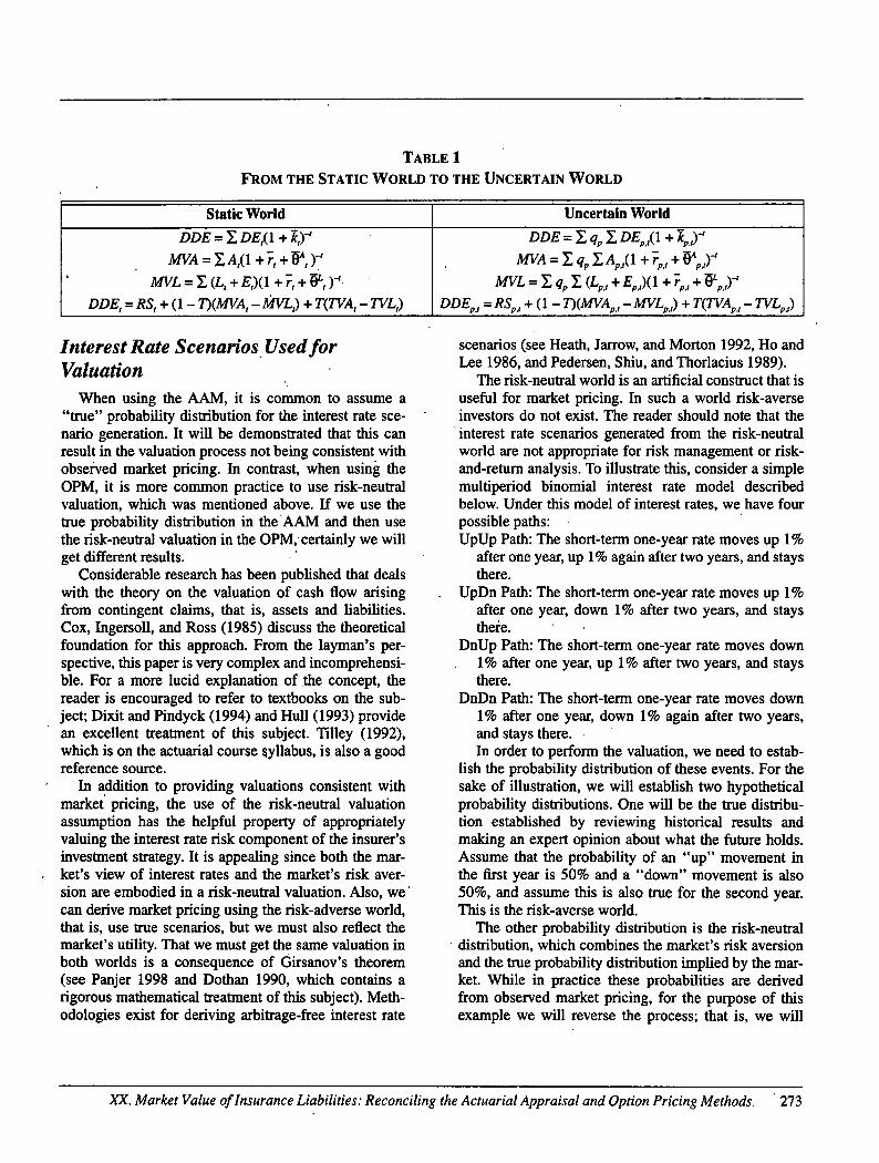
TABLE 1

FROM THE STATIC WORLD TO THE UNCERTAIN WORLD

Static World Uncertain World

DDE = ~ DE,(1 + k,)-'

MVA = ~ At( I + "rt + ~ t ) -t

MVL = Z (L, + E,)(1 + r, + rJL, ) -~.

DDE, = RS, + (1 - T)(MVA,- MVL,) + T(TVA,- TVL,)

DDE = ~. qp ~. DEp.,(1 + kp,,)"

MVA = Y~ qp ~, Ap.,(1 + rp,, + OAp.t)

MVL = • qp E (Lp., + ep,,)(1 +rp., + ~p.,)-'

DDEp., = RSp., + (1 - T)(MVAp.,- MVLp.t) + T(TVAn, ' - TVLp.t)

Interest Rate Scenarios Used for Valuation

When using the AAM, it is common to assume a "true" probability distribution for the interest rate scenario generation. It will be demonstrated that this can result in the valuation process not being consistent with observed market pricing. In contrast, when using the OPM, it is more common practice to use risk-neutral valuation, which was mentioned above. If we use the true probability distribution in theAAM and then use the risk-neutral valuation in the OPM,' certainly we will get different results.

Considerable research has been published that deals with the theory on the valuation of cash flow arising from contingent claims, that is, assets and liabilities. Cox, Ingersoll, and Ross (1985) discuss the theoretical foundation for this approach. From the layman's per- spective, this paper is very complex and incomprehensi- ble. For a more lucid explanation of the concept, the reader is encouraged to refer to textbooks on the subject; Dixit and Pindyck (1994) and Hull (1993) provide an excellent treatment of this subject. Tilley (1992), which is on the actuarial course syllabus, is also a good reference source.

In addition to providing valuations consistent with market' pricing, the use of the risk-neutral valuation assumption has the helpful property of appropriately valuing the interest rate risk component of the insurer's investment strategy. It is appealing since both the market's view of interest rates and the market's risk aversion are embodied in a risk-neutral valuation. Also, we' can derive market pricing using the risk-adverse world, that is, use true scenarios, but we must also reflect the market's utility. That we must get the same valuation in both worlds is a consequence of Girsanov's theorem (see Panjer 1998 and Dothan 1990, which contains a rigorous mathematical treatment of this subject). Meth- odologies exist for deriving arbitrage-free interest rate

scenarios (see Heath, Jarrow, and Morton 1992, Ho and Lee 1986, and Pedersen, Shiu, and Thorlacius 1989).

The risk-neutral world is an artificial construct that is useful for market pricing. In such a world risk-averse investors do not exist. The reader should note that the

interest rate scenarios generated from the risk-neutral world are not appropriate for risk management or risk- and-return analysis. To illustrate this, consider a simple multiperiod binomial interest rate model described below. Under this model of interest rates, we have four possible paths: UpUp Path: The short-term one-year rate moves up 1%

after one year, up 1% again after two years, and stays there.

UpDn Path: The short-term one-year rate moves up 1% after one year, down 1% after two years, and stays there.

DnUp Path: The short-term one-year rate moves down 1% after one year, up 1% after two years, and stays there.

DnDn Path: The short-term one-year rate moves down 1% after one year, down 1% again after two years, and stays there. In order to perform the valuation, we need to estab-

fish the probability distribution of these events. For the sake of illustration, we will establish two hypothetical probability distributions. One will be the true distribution established by reviewing historical results and making an expert opinion about what the future holds. Assume that the probability of an "up" movement in the first year is 50% and a "down" movement is also 50%, and assume this is also true for the second year. This is the risk-averse world.

The other probability distribution is the risk-neutral • distribution, which combines the market's risk aversion

and the true probability distribution implied by the market. While in practice these probabilities are derived from observed market pricing, for the purpose of this example we will reverse the process; that is, we will

XX. Market Value of Insurance Liabilities: Reconciling the Actuarial Appraisal and Option Pricing Methods. 273

assume a set of risk-neutral probabilities and then derive market prices from these probabilities. There- fore, for this example, take as given that the market is assuming that the risk-adjusted probability of an "up" move is 75% per year and the probability of a "down" move is 25% per year. The true and risk-neutral probabilities for each path are shown in Table 2.

The risk-neutral probabilities imply market prices, that is, a yield curve. The detailed development of this yield curve, while it is relatively simple, is not shown here. This yield curve is shown in Table 3 for both the risk-free and the risky yield curves, assuming a risk premium of 0.70%.

We can use Tables 2 and 3 to derive expected returns for bonds of various maturities by calculating total returns for each possible path and weighting these with the probabilities in Table 2. These expected returns are shown in Table 4. It should be obvious as to why we cannot use the risk-neutral world for risk-and-return analysis, because expected returns are the same regard- less of risk.

Table 5 illustrates that the true probability distribution (without adjustment for utility) is not appropriate for valuation. The table shows the pathwise present values of two investment strategies: Strategy no. 1 Invest $1,000 today (t = 0) in a four-year

par bond earning a par coupon of 6.28%. Strategy no. 2 Invest $1,000 today (t = 0) in a one-year

par bond earning a par coupon of 5.70%. At t = 1 reinvest the maturing proceeds in a three-year par coupon bond. Thus, both strategies have the same time horizon. The three-year coupon bond yield is 7.01% and 5.02% for the UpUp/UpDn and DnUp/ DnDn scenarios, respectively. Table 5 shows the valuations for each strategy in

each word. The pathwise values are the same for each word and are calculated by discounting the asset cash flow at the one-period risk-free rate plus the 0.70% risky premium. The valuations are obtained by weighting the pathwise values with the probabilities from Table 2.

Risk-neutral valuation correctly values the interest rate risk for both strategies, and since assets are fairly priced, one strategy does not have an advantage over the other on a risk-adjusted basis. For the true valuation, this is not the case because risk is not being valued using the market's assumptions; that is, it is ignoring the market's utility. For strategy no. 2, the true valuation

prices the initial one-year investment correctly at 1,000.00; however, it values the future reinvestment at 8.28 for a total of 1,008.28 for the strategy.

The Cost of Capital Assumption A critical assumption is the cost of capital that is

used to discount free cash flow. It may or may not reflect the market's assumption. For example, it may reflect a company's profitability target for a particular transaction. It may be partially based on the markets since it reflects the company's cost of raising capital in the market. However, if the riskiness of the transaction differs from risks that the company has historically underwritten, then the transaction could be mispriced.

TABLE 2

SCENARIO PATH PROBABILITIES

Path True Risk-Neutral"

UpUp 0.25 0.56 UpDn 0.25 0.19 DnUp 0.25 0.19 DnDn 0.25 0.06

aThe calculation is as follows 0.56 = 0.75 × 0.75, 0.19 = 0.75 × 0.25, 0.19 = 0.25 × 0.75, and 0.06 = 0.25 × 0.25.

TABLE 3

YIELD CURVE

Maturity Risk-Free Risky Assets

5.00% 5.24 5.47 5.58 5.65

5.70% 5.94 6.17 6.28 6.35

TABLE 4

EXPECTED RETURNS

Maturity True Risk-Neutral

5.70% 6.17 7.07 7.92 8.73

5.70% 5.70 5.70 5.70 5.70


TABLE 5 ASSET VALUATION: TRUE VERSUS RISK-NEUTRAL

UpUp UpDn DnUp DnDn Risk- Path Path Path Path True Neutral

Strategy 1 979.29 1011.31 1029.49 1064.00 1021.02 1000.00 Strategy 2 991.91 1024.26 - 951.52 1025.43 1008.28 1000.00

An appropriate cost of capital assumption may be selected that truly reflects the riskiness of free cash flow; however, it may be a static assumption that does not vm'y by scenario. A refinement would be to set the cost of capital equal to the risk-free interest rate plus a fixed risk premium. While a dynamic cost of capital assumption would be an improvement, it may still not reflect the riskiness of the transaction, sin.ce it may not adequately reflect leverage. By leverage I mean the amount of liabilities relative to the 'amount of equity. The degree of leverage will be affected by the amount of RBC that is held and the extent of conservatism in the statutory reserve basis. Moreover, leverage will vary over time and by scenario: that is, leverage is dynamic.

Modigliani and Miller (1958 and 1963), in their landmark papers, derived the following expression for the leverage-adjusted cost of capital, which they called Proposition II:

k L = k + ( k - ~ D .

Here k is the cost of capital of the unlevered firm, d is the cost of debt, D is the market value of the firm's debt, and E is the market value of the firm's equity. This expression ignores taxes and is derived by assuming perfect market competition. It can be rewritten as

k L = k(D + E) - d ( D ) . E

If we define A as the market value of the assets of the firm, then A = D + E, and we can rewrite the equation above as

k L _ k (A) - d(D)

A-D

This equation shows that the leverage-adjusted cost of capital is a weighting of the unlevered cost of capital

• and the cost of debt, where the weights are the market

value of the assets and the market value of the debtfl Using the terminology that we defined in Sections 3 and 4, that is, A is MVA, D is MVL, and k is i, then the above equation can be rewritten as

k L = ( i )MVA - ( d ) M V L M V A - M V L

(6.1)

For simplicity we are ignoring state and time subscripts. As in Section 4, we can express i, d, k, and ~ as the sum of the risk-free interest rate plus a risk premium:

i = r + O A, d = r + O d, k = r ~ - O k, and k L = r + O *L.

Equation (6.1) can be rewritten, in terms of risk premiums, as

0 kL (Oa)MVA - - (Od)MV'L = M V A - M V L .. (6.2).

Section 4 demonstrates that we can use the AAM to derive MVL by discounting the liability cash flows directly. If we use this direct methodology, Equation (4.3) defines the liability spread that, when added to the risk-free interest rate, can be used to discount liability cash flows. For simplicity and without loss of generality, we ignore subscripts. Equation (4.3) then becomes

0 L = 0 A R P M V L ' (6.3)

Equation (3.3) defines required profit (RP).'For simplicity and without loss of generality, we ignore risk-based capital..We also ignore taxes; however, here we do lose some generality. If we do this, the relation for R P is

RP = (k - i)(MVA - MVL),

• and this equation can be rewritten in terms of risk premiums: ,

R P = (0' - 0a)(MVA - MVL). (6.4)

XX. Market Value of Insurance Liabilities: Reconciling the Actuarial Appraisal and Option Pricing Methods 275

Substituting Equation (6.4) into Equation (6.3) for the liability spread, we obtain

Oz = 04 _ ( O k - Oa)( M V A - M V L ) M V L

which can be rearranged as

. . . . M V A (Ok) (MVA - M V L ) 0 L = ~,U")-~--V-~ M V L

If we multiply the numerator and denominator of the second term by (0A)MVA - (04)MVL, we obtain

OL . . . . M V A = I,t~') M V L

_ ( O k ) ( M V A - M V L ) [ ( O A ) M V A - (Od)MVL]

M V L [ ( O a ) M V A - (Od)MVL] '

which can be rearranged as

M V A (0 k. M V A - M V L ]

(Oa)(O e) M V A - M V L

+ , ( O a ) M V A _ ( O d ) M V L "

Note that the expression next to 0 k is the reciprocal of the leverage-adjusted cost of capital (see Equation 6.2). Therefore, we can rewrite the equation as

p.

From this expression we can clearly see that, when we apply the AAM and set the cost of capital equal to the leverage-adjusted cost of capital, the liability spread reduces to the debt spread:

~ = 0 e.

This last result shows that when the debt spread is used in the OPM, the valuation is equivalent to using the AAM and assuming a leverage-adjusted cost of capital. The result is considerably more complex if we include taxes. For a more rigorous derivation involving taxes, see Girard (1999).

7. Experience-Rated Products Another assumption that interacts with investment

strategy is a crediting strategy that depends on the portfolio's investment results. While this cannot be easily illustrated with the GIC example, it is fairly obvious that consideration of portfolio-crediting strategies in deferred annuities, universal life, or any experience- rated product presents special challenges. An extreme case of this interaction is a variable annuity in which liabilities, except for fees, expenses, and cost of capital, are 100% specified by the asset strategy.

For such products we need to make a distinction between how liabilities are defined and the valuation process. If liabilities are defined in terms of the assets that fund them, then the liability cash flow will be a function of these assets and the investment strategy.

Despite this linkage with the assets, the conclusions contained in this paper are still valid and applicable to such products, admittedly less useful. DDE can be decomposed into its parts and valued in components, the cost of capital should be leverage adjusted, and risk- neutral assumptions should be used. The ability to decompose DDE into its components should not be taken to mean that liabilities can always be valued independently of the assets. To the extent that liability cash flow is defined by the asset strategy, this inter-action needs to be modeled and reflected in liability valuations. In the extreme situation when all the asset experience is passed along to policyholders (for example, variable annuities and separate accounts), the liabilities may indeed be the assets.

8. A GIC Example Consider an example in which the product is a GIC

and we wish to evaluate six investment strategies with very different interest rate and credit risk exposures while keeping other risks unchanged. For this example, we will use the same interest rate scenario paths created in Section 6, that is, Up-Up, Up-Down, Down-Up, and Down-Down: Liability: $1,000 four-year simple GIC with a 5.00%

interest rate. In a simple GIC interest is paid annu- ally.

Strategy no. 1: Initially invest in a 6.28% yielding par bond maturing in four years.

276 Financial Report ing Section Monograph

Strategy no. 2: Initially invest in a 5.70% yielding one- year par bond. Repeat this year after year at the then market interest rates.

Strategy no. 3: Initially invest in a 5.70% yielding one- year par bond. At the end of the first year invest all cash in a three-year par bond at the then market interest rates.

Cost of capital: Assume that the cost of capital is the risk-free interest rate plus 7%. At t = 1, the cost of capital is 12% for all scenarios. For t > 1, the cost of capital varies with the risk-free rate, but the risk premium is kept constant for all scenarios.

• Taxes: 35% of taxable income. • Required surplus: 3% of statutory liabilities. Operating expenses:. 0.10% per year. Product assets: Risk-free interest rate plus0~70%, net of

expected defaults and investment expenses. Surplus assets: Risk-free interest rate plus 1.00%, net of

expected defaults and investment expenses. Asset accounting basis: Statutory = tax = historical

amortized cost method. GIC accounting basis: Statutory interest rate = 4.50%,

and tax interest rate -- 5.50%. The results of the valuation for these three strategies,

decomposed into its constituent parts, are shown in Table 6.

The DDEs are calculated by discounting free cash flows at the cost of capital. We can also derive the

DDEs by applying Equation (4.1). For strategy no. 1, 65.49 = 30 + (1 - 0.35)(1038.96 - 1003.46) + (0.35) (1017.94 - 982.47). The same is true for the other two strategies. Recall that MVA includes the valuation of both initial assets and future reinvestment assets. In Table 6, these two components are shown separately. Assuming the true distribution, the valuations of assets, liabilities, and equity vary with investment s.trategy. The asset valuation also produces the absurd result that future reinvestment for strategy no. 3 has a value of $8.39. This is an unreasonable result because future investments will be purchased at market prices and should have a zero value.

Table 7 illustrates what happens when we use risk- neutral valuation. The asset valuation does not vary with investment strategy, but both the liability valuation and discounted distributable earnings do vary with strategy. Moreover, the use of risk-neutral valuation has reduced the degree of variation in the valuations of liabilities and equity. The remaining variation is due to not recognizing leverage, which varies for each strategy. We can take leverage into account by using a leverage- adjusted cost of capital in the valuation. Alternatively, we can simply discount liability cash flows at the risk- free rate plus a credit spread minus an adjustment for taxes (see Girard 1999).

TABLE 6 DDE DE¢OMPOSrrION: USING TRUE DISTRmUTmN

Required surplus

Initial product assets Future reinvestment

M.V. of liabilities

Tax value of assets

Tax value of liabilities

DDE

Strategy 1 Strategy 2 Strategy 3 Cash Matching Short Term Initially Short Term

30.00

1038.96

.0.00

1003.46

1017.94 982.47

65.49

30.00 1017.94

0.00

1000.67 1017.94

982.47 53.64 "

30.00

1017.94

8.39

1002.00

1017.94 982.47

58.23

XX. Market Value of lnsurance Liabilities: Recohciling the Actuarial Appraisal and Option Pricing Methods 277

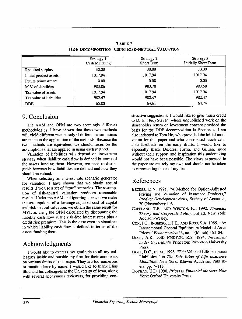
TABLE 7

DDE DECOMPOSITION: USING RISK-NEUTRAL VALUATION

Required surplus

Initial product assets

Future reinvestment

M.V. of liabilities Tax value of assets

Tax value of liabilities

DDE

Strategy 1 Strategy 2 Strategy 3 Cash Matching Short Term Initially Short Term

30.00

1017.94

0.00

983.06 1017.94

982.47

65.08

30.00

1017.94

0.00

983.78

1017.94

982.47

64.61

30.00

1017.94

0.00

983.58

1017.94

982.47

64.74

9. Conclusion The AAM and OPM are two seemingly different

methodologies. I have shown that these two methods will yield different results only if different assumptions are made in the application of the methods. Because the two methods are equivalent, we should focus on the assumptions that are applied in using each method.

Valuation of liabilities will depend on investment strategy when liability cash flow is defined in terms of the assets funding them. However, we need to distinguish between how liabilities are defined and how they should be valued.

When selecting an interest rate scenario generator for valuation, I have shown that we obtain absurd results if we use a set of "true" scenarios. The assumption of risk-neutral valuation produces reasonable results. Under the AAM and ignoring taxes, if we make the assumptions of a leverage-adjusted cost of capital and risk-neutral valuation, we obtain the same result for MVL as using the OPM calculated by discounting the liability cash flow at the risk-free interest rates plus a credit risk premium. This is the case even in situations in which liability cash flow is defined in terms of the assets funding them.

Acknowledgments I would like to express my gratitude to all my col-

leagues inside and outside my firm for their comments on various drafts of this paper. They are too numerous to mention here by name. I would like to thank Elias Shiu and his colleagues at the University of Iowa, along with several anonymous reviewers, for providing con-

structive suggestions. I would like to give much credit to D. E. (Ted) Steven, whose unpublished work on the shareholder return on investment concept provided the basis for the DDE decomposition in Section 4. I am also indebted to Tom Ho, who provided the initial moti- vation for this paper and who contributed much valu- able feedback on the early drafts. I would like to especially thank Dolores, Justin, and Gillian, since without their support and inspiration this undertaking would not have been possible. The views expressed in the paper are entirely my own and should not be taken as representing those of my firm.

References BECKER, D.N. 1991. "A Method for Option-Adjusted

Pricing and Valuation of Insurance Products," Product Development News, Society of Actuaries, 30 (November): 1--6.

COPELAND, T.E., AND WESTON, EJ. 1992. Financial Theory and Corporate Policy, 3rd ed. New York: Addison-Wesley.

Cox, J.C., INGERSOLL, J.E., AND ROSS, S.A. 1985. "An Intertemporal General Equilibrium Model of Asset Prices," Econometrica 53, no. - (March):363-84.

Dixrr, A.K., AND PINDYCK, R.S. 1994. Investment under Uncertainty. Princeton: Princeton University Press.

DOLL, D.C., ET AL. 1998. "Fair Value of Life Insurance Liabilities," in The Fair Value of Life Insurance Liabilities. New York: Kluwer Academic Publish- ers, pp. 7-113.

DOTH~'4, U.D. 1990. Prices in Financial Markets. New York: Oxford University Press.


FtNANCtAL AccourcrINo STANDARDS BOARD. 1993. "Accounting for Certain Investments in Debt and Equity Securities," Statement of Financial Accounting Standards No. 115. Norwalk, Conn.: .FASB.

GIRARD, L.N. 1999.. "Market Value of Insurance Liabil- ities and the Assumption of Perfect Markets in Val- uation," The Fair Value of Life Insurance Liabilities. New York: Kluwer Academic Publish- ers, in press.

GLrINN, P.L., BAreD, P.S., AND WEINHOFF, S.J. 1991. ".What Is a Life Company Worth?" Record of the

• Society of Actuaries 17, no. 4B:2251-74: HEATH, D., JARROW, R., AND MORTON; A. 1992. "Bond

Pricing and the Term Structure of the Interest Rates: A New Methodology," Econometrica 60:77-105.

HO, T.S.Y., AND LEE, S.B. q986. "'Term StrucUire Movements and Pricing Interest Rate Contingent Claims," Journal of Finance 41:1011-29.

HULL, J.C. 1993. Options, Futures, and Other Deriva- tive Securities, 2nd ed. Englewood Cliffs, N.J.: Prentice Hall.

MERFELD, T.J. 1995. "Market Value and Duration Esti- • mates of Interest Sensitive Life Contracts," ARCH 2:95-121.

MERTON, R.C. 1992. Continuous-Time Finance, revised ed. Cambridge, Mass.: Blackwell Publishers.

MODIOL.IANI, F., AND MILLER, M.H. 1958. "The Cost of Capital, Corporation Finance, and the Theory of Investment," American Economic Review 48, no. 3:261-97.

MODIGLIANI, F., AND MILLER, M.H. 1963. "Corporate Income Taxes and the Cost of Capital: A Correc- tion," American Economic Review 53:433--43.

PANJER, H., ed. 1998. Financial Economics: With Applications to Investments, Insurance rind Pen- sions. Schaumburg, IlL: Actuarial Foundation.

PEDERSEN, H.W., SHIU, E.S.W., AND THORLACIUS, A.E. 1989. Arbitrage-Free Pricing of Interest-Rate Con- tingent Claims,"-Transactions of the Society of Actuaries XLI:231-65.

TnOMr'SON, W.J., MILLER, S.K., Am) P.aCOIERt, A.A.' 1992. "Merger and Acquisition Topics," Record of

• the Society of Actuaries 18, no. 1B:473-95. TILLEY, J.A. 1992. "An Actuarial Layman's Guide to

Building Stochastic Interest Rate Generators," Trans- actions of the Society of Actuaries XLIV:509--64.

Tt.Wa~R, S.H. 1978. "Actuarial Appraisal Valuations of Life Insurance Companies," Transactions of the Society of Actuaries XXX: 139-60.

Appendix

Proof by Induction Of the DDE Decomposition

All terms below are as defined in Section 4. For. t >_ N, the proof is trivial. The decomposition

holds because all terms are zero; that is, there is no cash flow for t > N. Under the induction argument, assume the decomposition holds for some t '; N and then show that the decomposition must also hold for t - 1.'

Wecan rewrite, the definition of .MVA,_,, Equation 0)6), as

A, = ( i,)MVA,_~ - AMVA,_~. (A1)

Substitute Equation (A1) into Equation (1)2) for investment income,

lit = (i,)MVAt_ I - AMVAt_~ + A S V A t _ I , " (A2) '

and substitute Equation (A2) into Equation (I)3) for net income,

I t = [(i)MVAt_ 1 - AMVAt_ , + ASVAt_ l

+ (I)RS,_~ : 'L , -ASVL,_ t -Et](1 -7) -TBAt_ ~. (A3)

Under the AAM, SVAt_ ~ = SVLt_ 1 because, in a free cash flow model, all excess assets are distributed, and all deficiencies result in a shareholder infusion in order to bring statutory assets equal to the level of statutory liabilities. Thus, ASVA,_, = ASVL,_ I , these terms cancel, and Equation (A3) becomes 2°

I t = [(it)MVA,_ ~ - AMVAt_ ~

+ O)RS,_I - L , - E,](1 - 7) - ATBA,_,. (A4)

We can rewrite the definition of MVLt~ t, Equation (D7), as

L, + E t = (i,)MVLt_ t L AMVLt_ t _ Rpt. (A5)

Substitute Equation (A5) into Equation (A4):

/t = [(/)RS,-I + (it)MVA,-, - AMVAt_I

- (it)MVL,_ , + AMVLj(1 - 7)

+ (1 - T ) R P t -TBAt_ , (A6)

and substitute the definition for RP, Equation 0)8); into Equation (A6):


It = [(j')RS,_ l + (i)MVA,_ I - AMVA,_ l

- (i ,)MVL,_ t + AMVL,_~](1 - T)

+ [k - j (1 - T)]RS,_~

+ (k - i,)(1 - T)MVA,_~ - AMVLt_I)

+ (k)TBA,_ 1 - ATBA,_ I.

Collect terms involving k, and note that terms involving i and j cancel:

It = (k)[RS,_ l + (1 - T)MVA,_ I

- MVL,_I) + TBA,_ I]

- (1 - T)(AMVA,_ l - AMVL,_I)

+ (i,)MVL,_~ + A M V L j ( 1 - T)

- ATBA,_ r (A7)

By definition, DE, = I, - ARS,_~, substitute Equation (A7) into this equation:

D E , = (k)[RS,_ 1 + (1 - T)(MVA,_ 1

- MVL,_I) + TBA,_ I] - JARS,_ I

+ (1 - T)(AMVA,_ l - AMVL,_ l)

+ ATBAt_t]. (A8)

By the induction argument,

D D E , = RS, + (1 - T)(MVA, - M V L , ) + TBA, . (A9)

Add Equation (A8) to Equation (A9) and eliminate terms that cancel:

D D E , + DE,

= (1 + k)[RS,_~ + (1 - T)(MVA,_~

- MVL,_I) + TBA,_~ ]. (A10)

and divide both sides of Equation (A10) by (1 + k):

D D E , + D E , - R S , _ 1

l + k

+ (1 - T)(MVA,_ I - MVL,_ I)

+ TBA,_ I •

Note that the left-hand side is DDE,_~ (see Equation D5), and the proof is complete, r7

End Notes 1. It will be shown that these differences can be rec-

onciled. Their similarity is obscured by income taxes and complex accounting rules that define free cash flow.

2. The OPM is usually based on the concept of "risk- neutral" valuation. See the discussion in Section 6. The inclusion of a spread is the practical application of this concept to reflect that not all risks are modeled stochastically (for example, credit risk, model risk).

3. Becker (1991) suggests using an option-adjusted spread approach when using the AAM. Under such an approach, arbitrage-free interest rate scenarios of the risk-free rate are generated, and the residual risk is priced for by discounting the free cash flows at the risk-free rate plus an OAS. The OAS would reflect an appropriate market premium for risks other than interest rate risk.

4. For this purpose, the AVR and other reserves, which are surplus in their nature, are assumed to form part of the RBC requirement. The [MR is assumed to form part of policy statutory reserves. This arbitrary categorization is incidental to the major conclusions of this paper.

5. Note that in a free cash flow model all excess assets are distributed and all deficiencies are offset by capital infusions from shareholders. Therefore, immediately after distribution of free cash flow, the statutory value of assets (SVA) is always equal to the statutory value of liabilities (SVL). So, if TVA = SVA, T V L = SVL , and SVA = SVL , then it follows that TVA - TVL = 0.

6. For simplicity, this expression ignores the impact of unrealized gains or losses with respect to these assets, and this assumption is made throughout this paper. If this assumption is deemed material, it is possible to accommodate this refinement by introducing additional terms in Equation (3.2).

7. Here a future investment or reinvestment means an investment that will be purchased from cash flow at a future date.

8. Note that after-tax required profits plus taxes on such profits is equal to pretax required profits.

9. In theory, the cost of capital should vary with both state and time. In practice, this is usually not a critical assumption relative to all the other assumptions that are made, and a static cost of capital may be

280 Financia l Report ing Sect ion Monograph

more meaningful to a client for which the appraisal is being done.

10. The task force paper used in the deductive formula FVL = FVA - AV, where AV stands for appraisal value, FVA for fair value of assets, and FVL for fair value of liabilities. See Doll et al. (1998), p. 28.

11. The decomposition is still possible without this simplifying assumption; however, the formulation of the decomposition formula and the proof are made unnecessarily more complicated. Also recall that RS includts the AVR.

12. The values k andj are represented as constants over state and time. The decomposition still holds if these quantities are allowed to vary with state and time.

13. Policy loans effectively reduce policy obligations and are thus considered to be negative liabilities. Policy loans could also be viewed as assets, which is in accordance with the current statutory accounting paradigm. Doing so would result in unnecessarily inflating both MVA and MVL by exactly the same amount in the decomposition, and DDE would not be affected.

14. The relation would hold even ff the amount paid to purchase an asset did not equal the amount of the increase in invested assets. In this event the difference would be recorded in investment income, and the relation would hold. We are not aware of any situation like this within the current statutory accounting rules, so this would likely happen only if the statutory accounting rules were violated. Thus, the relation is general and is valid even when errors are made in financial reporting.

15. If the tax values of assets and policy liabilities are equal to the statutory values, the last term vanishes (see also footnote 5).

16. MVA is for product assets only. It is defined in the context of a static scenario or one scenario path sampled from all possible paths. It may be helpful to think of this quantity as the "pathwise forward

market value" for such path. The use of the term "market value" becomes clearer when we weight these values at the valuation date by the risk-neutral pathwise probabilities since the result is truly the market value. If the weighting is done with probabilities that are not the risk-neutral probabilities, then the use of the term "market value" may be

• inappropriate. Note that under risk-neutral valuation, the market value of future reinvestment and disinvestment is zero; but this is not necessarily the case if we use probabilities that are not risk-neutral. This comment is also applicable to the definition of MVL.

17. Professor David E Babbel of the Wharton School, University of Pennsylvania, made this comment at the "Fair Value of Insurance Liabilities" conference on December 7-8, 1995. Professor Babbel made his remarks while discussing the draft paper entitled "Fair Valuation of Life Insurance Com- pany Liabilities," which was authored by the American Academy of Actuaries Task Force•

18. In his article Becker uses the form rp. t + oasp., for the cost of capital kp.,. In practice, perhaps for simplicity and ease of explanation, a static cost of capital is often used.

19. Do not confuse this with WACC, which is the weighted average cost of capital. This is M&M Proposition 111, and it can be used to value investments (projects) in the levered firm. The WACC is a weighting of the leverage-adjusted cost of capital and the cost of debt.

20. The relationship ASVA,_~ = ASVL,_~ will not hold throughout the period, but it will hold at the end of the period after the free cash flow has been distributed for that period. Since, under the AAM, we are discounting free cash flow occun'ing at the end of the period, that it differs in between the beginning and the end of a period does not invalidate this important relationship.

' XX. Market Value of Insurance Liabilities: Reconciling the Actuarial Appraisal and Option Pricing Methods 281

Monograph - Chapter XX - SOA Financial Reporting Section ...

Documents

Transcript of Monograph - Chapter XX - SOA Financial Reporting Section ...