UNIVERSITY OF

ILLINOIS LIBRARY

AT URBANA-CHAMPAIGNBOOKSTACKS

Digitized by the Internet Archive

in 2011 with funding from

University of Illinois Urbana-Champaign

http://www.archive.org/details/monitoringpayabl1358gent

330

B385No. 1358 COPY 2

STX

BEBRFACULTY WORKINGPAPER NO. 1358

Monitoring Payables and Receivables

James A. Gentry

Jesus M. De La Garza

College of Commerce and Business AdministrationBureau of Economic and Business ResearchUniversity of Illinois, Urbana-Champaign

BEBRFACULTY WORKING PAPER NO. 1358

College of Commerce and Business Administration

University of Illinois at Urbana-Champaign

May 1987

Monitoring Payables and Receivables

James A. Gentry, ProfessorDepartment of Finance

Jesus M. De La GarzaDepartment of Civil Engineering

MONITORING PAYABLES AND RECEIVABLES

by

James A. GentryProfessor of Finance

University of Illinois at Urbana-Champaign

and

Jesus M. De La GarzaDoctoral Candidate

Department of Civil EngineeringUniversity of Illinois at Urbana-Champaign

MONITORING PAYABLES AND RECEIVABLES

Abstract

Financial managers ara interested in monitoring the performance of

receivables and payables with an objective of increasing the speed of

cash inflows and reducing the speed of cash outflows. To accomplish

this mission, management must understand the relationships that cause

changes in accounts receivable and accounts payable. An objective of

this paper is to expand Gentry and De La Garza's [3] model for moni-

toring accounts receivable in order to explain the causes of changes in

payables. Several examples are developed to show the operation of the

model. The primary contributions of the paper are the algorithms that

measure the causes of changes in the two working capital components;

and the interpretation of the relationships that link changes in sales

and purchases to the respective collection and payment patterns which

result in causing receivables and payables to change. The model should

be of value to financial managers, financial analysts and academic

researchers interested in the underlying causes of changes in the amount

and timino; of cash flows.

MONITORING WORKING CAPITAL COMPONENTS

Tracking the amount and timing of a firm's cash inflows and out-

flows is a primary task of financial managers and analysts. When

analyzing the causes of changes in the level and speed of cash inflows

and outflows, management and analysts monitor changes in accounts re-

ceivable and accounts payable vis-a-vis changes in sales and purchases

of raw materials. There are numerous finance oriented models that

focus on the control of accounts receivable, e.g., [1, 2, 3, 4, 5, 7,

8, 10, 11, 13, 14, 15, 18]. However, the literature related to manag-

ing and controlling accounts payable is found in leading textbooks such

as [6, 12, 16], Understanding the relationships that exist between

receivables and sales and between payables and purchases provides the

base for predicting and controlling cash inflows and outflows.

Conceptually, changes in receivables and payables are directly

related to a firm's cash inflows and outflows, therefore, changes in

their performance directly affects the value of the firm [9, 17]. A

model that determines the causes of change in receivables and payables

would provide valuable information in explaining changes in the value

of a firm. A primary objective of this paper is to develop such a

model. The paper extends the generalized model for monitoring accounts

receivable developed by Gentry and De La Garza (GD) [8]. Objectives of

this paper are to present a matrix of conditions that are responsible

for changes in accounts payable; to create a model that identifies and

measures the causes of changes in payables; to interpret functional

relationships between independent cash flow variables that cause changes

-2-

in payables and receivables and, finally, to show the contribution of

this information in managing the receivables and payables.

Payables Behavior

GD identified seven sets of conditions that were needed in order

to analyze changes in accounts receivable. These conditions were

conceptualized in a 3x3 matrix based on the trend of sales patterns

(S) and collection experience (CE). Exhibit 1 is a similar 3x3 matrix

used to identify the conditions that cause changes in payables. The

horizontal axis represents changes in payables due to changes in

purchasing patterns. Changes in purchases are in turn related to

changes in a firm's demand for a supplier's products. The vertical

axis reflects changes in payables related to the firm's payment

experience. These changes in payment experience are In turn related

to changes in the supplier's credit policies or the firm's own internal

payment policies.

Changes in the purchasing patterns refer to changes in the level

of purchases occurring on a month-to-month basis. The pattern and trend

in purchases can change because of seasonal, cylical or random events.

The firm's payment experience reflects its relationship with the

supplier, the credit terms and the collection behavior of the supplier.

Payment experience is characterized by the fraction of credit purchases

in a month that remain outstanding at the end of a subsequent month.

For example if the payment pattern for December is 80-25-5; it means

80% of December's purchases are outstanding as payables on December 31;

-3-

25% of November's purchases are outstanding as payables on December 31;

and 5% of October's purchases are outstanding on December 31.

A.n overview of the seven conditions shown in Exhibit 1 provides the

logic for the payable 's algorithm. In Condition 1, payables do not

change because there is no change in Che purchasing patterns or the

payment experience. Under Condition 2, 100% of the change in payables

is associated to a change in payment experience. For example, payables

can increase because of lienient collection practices of suppliers or

the firm stretches payments beyond the due date to its suppliers.

Condition 2 is a lengthening of the payment pattern which is a benefit

because the firm is able to extend its use of the supplier's trade

credit without any explicit cost for the use of the funds. This

extension has no affect on purchases. Alternatively, under Condition

2', payables can decrease because suppliers tighten their collection

practices or a firm pays before the due date. The result is a

reduction in a firm's payment experience which has a cost because full

utilization was not made of the credit period. This reduction has no

affect on the firm's purchasing patterns.

Condition 3 is the opposite extreme of Condition 2, where 100% of

the change in payables can be attributed to a change in the demand for

goods from suppliers. Condition 3 reflects an increase in payables

caused by an increase in purchases. Under Condition 3', there is a

decrease in payables that is solely associated with a decrease in

purchases. In Condition 3 or 3', the increase or decrease in payables

did not affect supplier credit terras and/or collection behavior.

-4-

Conditton 4 depicts the case where payables increase because of

lenient collection practices by suppliers or the firm receiving credit

stretches on its payments. These practices have a spillover effect on

purchases which, in turn, is responsible for an increase in payables.

Simultaneously, an increase in the demand for supplier goods contributes

to an increase in purchases. The demand for additional supplier goods

results in a further increase in payables, which can spilLover and

cause a further relaxation in collection practices by suppliers or a

stretching of the firm's payments, i.e., a lengthening in payment

experience. In summary, an increase in payables can be a combination

of a pure purchasing effect, a pure payment effect and a joint inter-

action effect between purchases and payment. Under Condition 4, we

observe that both the purchasing pattern effect and the payment experi-

ence effect are so positioned as to cause payables to increase. \n

example of Condition 4 is a manufacturer that experiences an increase

in demand and in turn expands its purchases from the supplier. The

supplier responds by relaxing collection practices because of increased

business and allows the manufacturer to delay payment for the goods.

Or alternatively, a supplier relaxes its collection policies which

encourages a manufacturer to increase the size and/or frequency of its

orders for goods. The result of these two examples is an increase in

payables attributable to three effects—purchasing, payment and joint.

The circumstances under Condition 5 are opposite those in Condition

4. A tightening of collection procedures by a single dominant supplier

may result in the manufacturing firm having to accelerate its payments

for the goods received. At the same time, the firm may reduce its

-5-

purchases from the supplier because of the shortened credit period or

alternatively, it may either substitute a lower cost alternative

product or reduce the need for the supplier's product. Because both

payment experience and purchasing patterns are positioned to cause

payables to decline, we observe that a segment of the decrease in

payables is caused by a joint interaction between payment experience

and purchases. The interaction of more rapid payment and declining

purchases creates a joint effect. Thus under conditions of tightened

credit practices from a supplier, we are likely to observe payables

declining because of a reduction in payment experience, a reduction in

purchases and a joint effect.

Under Condition 6 and 7, opposite forces are interacting that

create a moderating influence. Under Condition 6, purchases are down

because of a decline in sales which results in lower payables, but

lenient collection practices by the supplier cause payables to decline

less rapidly than purchases or possibly to increase. These are

opposing interaction effects between the two forces. The size and

direction of the change in the payables is dependent on whether the

decline in purchases has greater effect than the lengthened payment

experience. Under Condition 7, tightened credit practices result in

lower payables, but increased demand causes purchases to increase. As

in Condition 6, there are opposing interaction effects with the

payment experience causing the change in payables to increase less

rapidly than the purchases or possibly to decline. The size and

direction of the change in payables depends on whether the increase in

purchases is more prominent than the influence of the tightened

-6-

collection practices of the supplier. In summary, from the perspec-

tive of the accounts payable manager and taking into account the pur-

chase, payment and joint effects, Condition 4 is the most attractive

outcome of the seven scenarios in Exhibit 1 and Condition 5 is the

least preferred outcome.

Payables Model

Using the GD model as an anchor, we developed separate algorithms

for measuring the purchasing pattern effect (PPE), the payment

experience effect (PEE), and the joint effect for payables (JEP) for

each of the seven conditions. The algorithm for each condition is

presented in Exhibit 2. Examples are developed in Exhibit 3 to show

the operation of each algorithm and to determine the contribution of

the PPE, PEE and JEP to the changes in payables. The information used

in each of the examples is in Exhibit 3.

Exhibit 3 shows there has been a $7 million increase ($78 million

- $71 million) in payables between months 3 and 6. What was the

contribution of the purchasing, payment and joint effects to the $7

million change in payables? The example shows the payables in month t

are composed of current purchases in month t and purchases made in the

two preceding months, t-1 and t-2. To calculate the contributions to

payables for months t, t-1 and t-2, it is necessary to multiply the

purchases in month t times the payment pattern in that month and repeat

the process for months t-1 and t-2. That is, the $71 million in pay-

ables in month 3 is composed of $40 million from month t ($80 million x

.50), $22 million from month t-1 ($110 million x .20) and $9 million

from month t-2 ($90 million x .10).

-7-

To calculate the separate effects causing changes in payables, it

is necessary to determine the value that months t, t-1 and t-2 contri-

bute to the total payables in month t. The first step is to determine

the change in purchases that occurred between period t-2 in month 3 and

period t-2 in month 6. Exhibit 3 shows purchases decreased $10 million

($80 million - $90 million) and the payment pattern was unchanged at

.10. This decrease was caused by a decline in purchases, or a

purchasing pattern effect (PPE), which is Condition 3 in Exhibit 2.

The next step is to determine the contribution of period t-1 to total

payables in month t. Exhibit 3 shows there was no change in purchases

or payment patterns which is Condition 1. Finally the contribution

month t makes to total payables is a lengthening in the payment pattern

from .5 to .6 between months 3 and 6 and no change in purchases, which

is Condition 2. Using the respective algorithm for each condition,

the contribution of each time period to the total payables is shown in

Exhibit 4.

Exhibit 4 shows the $7 million increase in payables between months

3 and 6 was caused by an $8 million lengthening in the payment

experience of the firm and a decrease in purchases which reduced

payables by $1 milLion. When the two effects are combined, they equal

the $7 million ($8 million - $1 million) change in payables. In a

relative context, the payment experience effect contributed 114.28%

(8/7) of the change in payables between months 3 and 6, while

purchasing contributed a -14.28% (- 1/7) to the change in payables.

Exhibit 4 presents an example that determines the contribution of

the PPE, PEE and JEP effects that cause a $4 million increase in pay-

ables between months 3 and 9. The information from months 3 and 9

that is used in the algorithms for Conditions 4, 5 and 6 is presented

in Exhibit 3, The Condition 4 algorithm is used to determine the

causes of the changes in payables between period t-2 for months 3 and

9. The Condition 6 algorithm is used to solve for the causes of change

in payable effects for period t-1 in months 3 and 9 and the Condition 5

algorithm is used for period t in months 3 and 9. Exhibit 4 summarizes

the results which shows the purchasing pattern effect was $-7 million

($1, $-4 and $-4 million for the respective periods); the payment experi-

ence pattern was $11 million ($9, $9 - $7 million for the respective

periods) and the joint effect of zero ($1 million in t-2 and $-1 million

in t). Thus the payment effect contributed -175% (-7/4 million) of

the $4 million change in payables between periods 3 and 9 and 275%

(11/4) was attributed to the payment experience pattern.

There was an $11 million reduction in payables between the third

and twelfth months. Exhibit 4 shows Condition 7 explains the change

in payables for period t-2 and t and Condition 3 for period t-1. The

payment effect contributed a -172.72% (-19/11) of the $11 million decline

in payables, while the purchasing experience offset a +72.72% of the

decline. These examples show that there are periods when the

purchasing, payment and joint effects cause payables to increase and,

alternatively, the same three effects cause payables to decrease.

Understanding this phenomenon provides insights for management and

financial analysts.

-9-

Interpreting Relationships

Although the algorithms for determining the cause of changes in

payables and receivables have been presented and interpreted, our

final objective is to establish a solid grounding of the key rela-

tionships that underlie the analysis. Exhibit 5 is an extension of the

original matrix in Exhibit 1 and shows graphically how changes in

accounts payable (AAP) are caused by changes in purchases ( AP ) and

payment experience (APE) and how changes in accounts receivable (A\R)

are related to changes in sales (AS) and changes in collection ex-

perience (ACE). A brief explanation of Exhibit 5 will assist the

interpretation of these key relationships.

In Cell 1 of Exhibit 5, we observe no change in either of the

working capital components, because there is no change in any of the

independent or dependent variables. That is, the slope in accounts

payable (MP) is zero because the change in purchases ( AP ) and payment

experience (APE) are zero.

In Cell 2 of Exhibit 5 the slope of P and S are unchanged from the

previous period, therefore, the increase in the trend of AP and AR is

caused by the lengthening of the payment experience (APE) and the

deterioration in the collection experience ( ACE ) , respectively. Cell

2' reflects no change in P or S, but a reverse set of conditions for

payment and collection experience causes the trend of the two working

capital components to decrease. From the perspective of monitoring

accounts payable and observing a slowdown in outflows, Cell 2 provides

better performance results than Cell 2'. However, from the

-10-

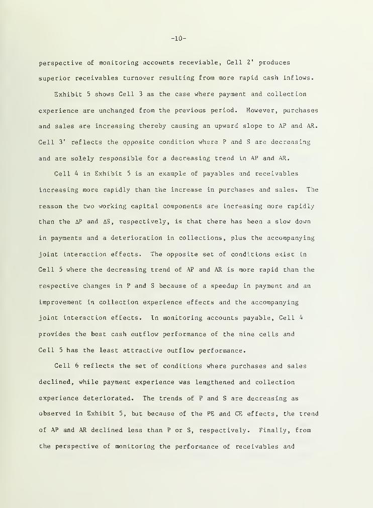
perspective of monitoring accounts receviable, Cell 2' produces

superior receivables turnover resulting from more rapid cash inflows.

Exhibit 5 shows Cell 3 as the case where payment and collection

experience are unchanged from the previous period. However, purchases

and sales are increasing thereby causing an upward slope to AP and AR.

Cell 3' reflects the opposite condition where P and S are decreasing

and are solely responsible for a decreasing trend in AP and AR.

Cell 4 in Exhibit 5 is an example of payables and receivables

increasing more rapidly than the increase in purchases and sales. The

reason the two working capital components are increasing more rapidly

than the AP and A3, respectively, is that there has been a slow down

in payments and a deterioration in collections, plus the accompanying

joint interaction effects. The opposite set of conditions exist in

Cell 5 where the decreasing trend of AP and AR is more rapid than the

respective changes in P and S because of a speedup in payment and an

improvement in collection experience effects and the accompanying

joint interaction effects. In monitoring accounts payable, Cell 4

provides the best cash outflow performance of the nine cells and

Cell 5 has the least attractive outflow performance.

Cell 6 reflects the set of conditions where purchases and sales

declined, while payment experience was lengthened and collection

experience deteriorated. The trends of P and S are decreasing as

observed in Exhibit 5, but because of the PE and CE effects, the trend

of AP and AR declined less than P or S, respectively. Finally, from

the perspective of monitoring the performance of receivables and

-11-

speeding up the inflow of cash, Cell 6 is inferior to any of the other

eight cells.

Because of a speedup in payment experience and the improvement: in

collection experience, Cell 7 shows the trendlines for AP and AR are

not increasing as rapidly as their counterpart variables, P and S.

From the perspective of monitoring the performance of receivables and

improving the timing and amount of cash inflow, Cell 7 is superior to

any of the other eight cells in the matrix.

Exhibit 5 provides a useful framework for financial managers,

analysts and academic researchers to identify quickly the sets of

conditions and variables responsible for changing the cash converti-

bility trend of AP and AR. As indicated the cells in Exhibit 5 high-

light the location as to where the worst sets of conditions exist for

increasing AP and AR, as well as the best set of conditions. Using

the cash conversion cycle as a benchmark, the best set of conditions

for payables are in the top row of Exhibit 5 and the best set of con-

ditions for receivables is the bottom row of Exhibit 5.

Conclusion

The model developed can be used to measure and analyze the condi-

tions that cause changes in payables and receivables. The respective

relationships that exist between purchasing and sales vis-a-vis payment

and collection experience patterns are the foundations for the

algorithms. Exhibit 5 provides a useful framework for financial

managers, analysts and academic researchers to analyze the causes of

changes in payables, receivables, cash flow and value of the firm.

-12-

Footnote

The algorithms for receivables are in Exhibit 2 of GD

-13-

References

1. W. Beranek, Analysis for Financial Decisions , Homewood, XL,

Richard D. Irwin, 1963.

2. M. D. Carpenter and J. E. Miller, "A Reliable Framework for

Monitoring Accounts Receivable," Financial Management (Winter1979), pp. 37-40.

3. R. M. Cyert, H. J. Davidson, and G. L. Thompson, "Estimation of

Allowance for Doubtful Accounts by Markov Chains," ManagementScienc e (April 1962), pp. 287-303.

4. R. M. Cyert and G. L. Thompson, "Selecting a Portfolio of CreditRisks by Markov Chains," Journal of Business (January 1968), pp.

39-46.

5. L. P. Freitas, "Monitoring Accounts Receivable," Management

Accounting (September 1973), pp. 18-21.

6. G. W. Gallinger, Liquidity Analysis and Management , Reading, MA,

Addison-Wesley Publishing Company, 1987.

7. G. W. Gallinger and A. J. Iff lander, "Monitoring Accounts ReceivableUsing Variance Analysis," Financial Management (Winter 1986), pp.69-76.

8. J. A. Gentry and J. M. De La Garza, "A Generalized Model forMonitoring Accounts Receivable," Financial Management (Winter1985), pp. 28-38.

9. J. A. Gentry and H. W. Lee, "An Integrated Cash Flow Model of the

Firm," Faculty Working Paper No. 1314, Bureau of Economic and

Business Research, University of Illinois, December 1986.

10. N. C. Hill and K. D. Riener, "Determining the Cash Discount in the

Firm's Credit Policy," Financial Management (Spring 1979), pp.68-73.

11. J. D. Kallberg and A. Saunders, "Markov Chain Approaches to

Analysis of Payment Behavior of Retail Credit Customers,"Financial Management (Summer 1983), pp. 5-14.

12. Donald E. Kieso and Jerry J. Weygandt , Intermediate Accounting,

Fourth Edition, New York, John Wiley & Sons, 1983.

13. G. H. Lawson, "The Mechanics, Determinants and Management of

Working Capital," Managerial Finance (No. 3/4 1984), pp. 12-25.

-14-

14. W. D. Lewellen and R. W. Johnson, "Better Way to Monitor AccountsReceivables," Harvard Business Review (May-June 1972), pp. 101-109.

15. W. D. Lewellen and R. 0. Edmister, "A General Model for AccountsReceivable Analysis and Control," Journal of Financial andQuant itative Analysis (March 1973), pp. 195-206.

16. W. B. Meigs, A. N. Mosich and C. E. Johnson, IntermediateAccounting , Fourth Edition, New York, McGraw Hill Book Company,

1978.

17. W. L. Sartoris and N. C. Hill, "A Generalised Cash Flow Approachto Short-Term Financial Decisions," Journal of Finance (May 1983),pp. 349-360.

18. B. K. Stone, "The Payment Pattern Approach to Forecasting andControl of Accounts Receivable," Financial Management (Autumn1976), pp. 65-82.

D/53

Exhibit 1

Sets of Conditions Responsible for Changes in Payables

Purchasing Patterns (P)

PaymentExperience(PE)

Lengthening ( +)

No Change (NC)

Reducing ( +)

UP( t)

No Change(NC) Down(

4 2 6

3 1 3'

7 2' 5

Exhibit 2

Algorithms for Measuring the Pattern EffectsThat Cause a Change in Payables

Condition

1

2, 2'

3, 3'

4

Descriptio n

NC in PE or P

t or + in PE and NC in P

(P. = P.)J i

t or 4- in P and NC in PE

t in PE and t in P

Type of

Effects

None

PEE

PPE

PPE

PEEJEP

Algorithm

APE x P

AP x PE

AP x PEj_

APE x ?iAP x APE

+ PE and 4- in P PPEPEE

JEP

AP x PEj

APE x p-

:

AP x APE

Legend

P

PE

NC

t or I

i

J

PPEPEEJEP

t in PE and I in P

4- in PE and t in P

Purchasing PatternsPayment ExperienceNo ChangeSee Exhibit 1

Oldest MonthCurrent MonthPurchasing Pattern EffectPayment Experience EffectJoint Effect for Payables

PPE

PEE

PPE

PEE

AP x PEj

APE X P:

AP x PE,

APE x Pi

Exhibit 3

Four Months of Information Used to Determine Payables

and the Separate Effects Causing Them to Change(In Millions of Dollars)

Th ree

Mo nth Moinths

Representing Include d Payment

Period t in Paya bles Purchases Patterns

(1) (2) (3) (4)

t-2 90 .10t-1 110 .20

3 t

t-2

t-1

80

80

110

.50

.10

.20

6 t

t-2

t-1

80

100

90

.60

.20

.30

9 t

t-2t-1

70

100

100

.40

.20

L2 t 100 .40

TotalMonthly AccountsContribution Payableto Payables in Monthin Period t Sum of Col

(5) = (3)x(4) (6)

9

22

40

8

22

48

20

27

28

20

40

71

75

60

0)

.-I

CU X>Xl CO4-1

CO

9) (Xl-i

3 03

05 4J

RJ CCU 3X C

Oo a ^4-1

CO C CO

E •^ ^-i

X i—l

4-1 co oH cu -a<r iu bo

o C U-l

j-> bo CO o•r-l i—

i

XX <U CJ 05

•H cX <u cu oX X 05 -H[d 4-1 3 r-<

CO i—

'

bO CJ —

'

d e•r-l 4-1

cn CO C3 X -r-l

4-1 v-'U-l

O 05

4-1

0) ar-H CU

a, <4-l

6 U-l

« wXW CU

CU

c Su

<:

CO

<u^H r-i

XCO 4-J

CU >, •r-1

bo (0 X>c a. e -hCO o xx c U Xcj •r-i u-i W|

co I

CU4_) H

4-) CJ X y^.1

c cu co a- 1

.^ U_l i-i >^ CxJ

O u-i o CO "-)

—) w U-l

cuCJ

c

(X ^l

4-1 01 CO

c -l-l 4-1

cu S-i CJ /~Jg cu CU W>^ cu u-i u!CO X U-l CUP- w wHbo i

C•Hco cCO l-l 4Jr- cu CJ /-^

"cj 4-1 cu m\S-i 4-1 U-i Cu 1

3 cd U-l Cu 1

a. (3- U2 v-^|

05

°H

4_) -^•H si-l

o CbO-Hl—l

4.) CU 4J•H CX CJ"3 >-, CU

C H u-i

O u-i

C_5 ^ W

lo!' i to 1 '

OS

oCS

o00

oco

ou-i

Io

I

o o • o^ OS I No •

X cmX . X

l VII

omo oas O r-~

X . X

WW Z CjJ

Cm O bJCw Z (5-

rn CN

CM —

i

I I

•rJ 05

CU CCU rH CU 05

bO xi cu xC CO 3 4J co co. co co«0 >|<J c 1 1 1 1

x CO cu o \0 vO sD \DCJ 0- po 7C

oOS

Ioo

^ oX O CN

o o

X •-s

oo •

I CO I

O I ocj cs o co o <r

—i .i o>oo

UJ li] CU Ldcu ua cd CuCu Cu >-j Cu

• p^

ii] u ii] aW Cu CjJ UCu Cu Cu !-)

•j^srsOvoioinio

CMI

col

o>

CO m<^ ON

mI

OS

i ll

OS CMI I

CO'OS '

I I-1

00 |00 I

oO CN O OOS • <f CO

X XX

^ o c ^ oO —i —i o mOS • H CO •

I I I I Io o o o oo • o o <r—

i

O — —

'

U Id Cd U HCu Cu Cu Cu udCu Cu Cu CU Cu

r-» r-«. co r~~ i~~

CMI

ro ro ro ro

CM CNI CM CM

(AP) Lengthening (|)

(Best)

(AR) Deteriorating (|)

(Worst)

Exhibit 5

Examples of Relationships that CauseChanges in Payables and Receivables

Purchasing or Sales Patterns

No Change

(Neutral)

$

Down (|)

(Worst)

6

PaymentExperience

or

Collection

Experience

No Change

(Neutral)

(AP) Reducing (|)

(Worst)

(AR) Improving ({)

(Best)

Slope of purchases or sales in period t

Slope of payables or receivables in period t

HECKMANBINDERY INC.

JUN95, 9 N MANCHESTER.

iounJ -To-Wearf,ND1ANA 46962