Monetary Policy Rules for an Open Economy

Nicoletta Batini*Richard Harrison**

andStephen P. Millard

January 2001

Abstract

The most popular simple rule for the interest rate, due to Taylor (1993a) is meant to inform monetarypolicy in economies that are closed. On the other hand, its main open economy alternative, i.e. Balls(1999) rule based on a Monetary Conditions Index (MCI), may perform poorly in the face of specifictypes of exchange rate shocks and thus cannot offer guidance for the day-to-day conduct of monetarypolicy. In this paper we specify and evaluate a comprehensive set of simple monetary policy rules thatare suitable for small open economies in general, and for the United Kingdom in particular. We do so byexamining the performance of a battery of simple rules, including the familiar Taylor rule and MCI-basedrules à la Ball. This entails comparing the asymptotic properties of a two-sector open-economy dynamicstochastic general equilibrium model calibrated on United Kingdom data under different rules. We findthat an inflation forecast based rule (IFB), i.e. a rule that reacts to deviations of expected inflation fromtarget, is a good simple rule in this respect, when the horizon is adequately chosen. Adding a separateresponse to the level of the real exchange rate (contemporaneous and lagged) appears to reduce thedifference in adjustment between output gaps in the two sectors of the economy, but the improvement isonly marginal. Importantly, an IFB rule, with or without exchange rate adjustment, appears robust todifferent shocks, in contrast to naïve or Balls MCI-based rules.

* Research Adviser, MPC Unit, Bank of England, Threadneedle Street, London EC2R 8AH, UnitedKingdom. Tel: +44 20 76014354. Fax: +44 20 76013550E-mail: nicoletta.batini@bankofengland.co.uk (corresponding author)

** Analyst, Monetary Assessment and Strategy Division, Bank of England, Threadneedle Street, LondonEC2R 8AH, United Kingdom. Tel: +44 20 76015662. Fax: +44 20 76014177.E-mail: richard.harrison@bankofengland.co.uk

Manager, Monetary Instrument and Markets Division, Bank of England, Threadneedle Street, LondonEC2R 8AH, United Kingdom. Tel: +44 20 76014115. Fax: +44 20 76015953.E-mail: stephen.millard@bankofengland.co.uk

We would like to thank Nicola Anderson, Larry Ball, Spencer Dale, Shamik Dhar, Rebecca Driver, ChrisErceg, Neil Ericsson, Jeff Fuhrer, Andy Levin, Bennett McCallum, Katherine Neiss, Edward Nelson,Athanasios Orphanides, Glenn Rudebusch, Chris Salmon, Anthony Yates and seminar participants at theBank of England for useful comments on earlier versions of this paper. Remaining errors, and the viewsexpressed herein are those of the authors and not of the Bank of England nor of the Bank of EnglandsMonetary Policy Committee. The work has still not been finalised and so results contained herein shouldonly be quoted with the permission of the authors.

2

1. Introduction

The literature on simple rules for monetary policy is vast.1 It contains theoreticalresearch comparing rules that respond to alternative intermediate and final targets,backward- and forward-looking rules, and finally, rules which include or excludeinterest rate smoothing terms. It also contains work on historical estimates of monetarypolicy rules for various countries.

However, the literature does not contain a thorough normative analysis of simple rulesfor open economies, i.e. for economies where the exchange rate channel of monetarypolicy plays an important role in the transmission mechanism.2 The most popularsimple rule for the interest rate due to Taylor (1993a) for example, was designedfor the United States and, thus, on the assumption that the economy is closed. And themain open economy alternatives, (for example, the rule by Ball (1999) based on aMonetary Conditions Index (MCI)), may perform poorly in the face of specific types ofexchange rate shocks and thus cannot offer guidance for the day-to-day conduct ofmonetary policy.3 So at present we only have a choice of ignoring the exchange ratechannel of monetary transmission completely (Taylor rule) or including it in an ad hocway that may not always prove right (MCI-based rules).

In this paper we specify and evaluate a family of simple monetary policy rules that maystabilize inflation and output in small open economies at a lower social cost thanexisting rules. These rules parsimoniously modify alternative closed- or open-economyrules to analyse different ways of explicitly accounting for the exchange rate channel ofmonetary transmission. We compare the performance of these rules to that of a batteryof existing rules when the model economy is buffeted by various shocks. The existingrules include the Taylor closed-economy rule, naïve MCI-based rules as well as BallsMCI-based rule, and inflation forecast-based rules. Some of the rules in the family weconsider appear to be robust across a set of different shocks, including shocks from therest of the world. This is in contrast to closed-economy rival simple rules, which ignorethe exchange rate channel of monetary transmission, and MCI-based rules, theperformance of which can be highly shock-specific.

To test the rules, we stylise the economy that we calibrate to UK data as a two-sector open-economy dynamic stochastic general equilibrium model. The export/non-traded sector split is important because it allows us to discern different impacts of thesame shock on output and inflation in the two sectors. Identification of sectoralinflation and output dynamics is a key element on which to base the design of efficientpolicy rules. More generally, it also makes it possible for the monetary authority toconsider the costs of price stabilization on each sector of the economy.

1 See Bryant et al (1993) and Taylor (ed.) (1999).2 Clarida, Gali and Gertler (1998, 2000) offer a wealth of empirical international evidence on monetarypolicy rules. Clarida (2000) employs the empirical framework of Clarida et al (1998, 2000) to explore theperformance of historical monetary policy rules in open economies. More recently, Clarida et al (2001)also compared optimal monetary policy in open versus closed economies. Using a structural, small openeconomy model they show that under certain standard conditions, the (optimal) monetary policy designproblem for the small open economy is isomorphic to the problem of the closed economy [] consideredearlier (Clarida et al (2001), p. 1, text in brackets added).3 See King (1997) and Batini and Turnbull (2000) on the potential flaws of MCI-based rules.

3

Because it is theoretically derived on the assumption that consumers maximise utilityand firms maximise profits, the model has a rich structural specification. This enablesus to contemplate shocks that could not be analysed in less structural or reduced formsmall macro-models.

In particular, with our model, we can examine the implications of shocks to aggregatedemand such as a shock to households preferences, or a shock to overseas output. Onthe supply side, we can consider shocks to overseas inflation. We can analyse theimpact of a relative productivity shock on the two sectors and investigate how thisaffects the real exchange rate by altering the relative price of non-tradables and exports.We can also look at the effects of a change in the price of imported intermediate goods.We can examine the effects of shocks to the foreign exchange risk premium. Finally,we can look at the implications of a monetary policy shock, both at home and abroad.

The ability to examine all these different shocks is important when comparingalternative policy rules for an open economy, because the efficient policy response tochanges in the exchange rate will typically depend on the shocks hitting the economy with different shocks sometimes requiring opposite responses. For this purpose oursmall economy general equilibrium model is sufficient. A two-country model wouldenable us to look at these same shocks, but we believe the small-economy assumptionis more realistic for the United Kingdom.

In short, this model is well suited to our analysis for three reasons. First it is astructural, theoretically based model. The structural nature of the model is importantbecause it implies that our policy analysis (i.e. comparison of different rules/regimes) isless subject to the Lucas critique than a reduced-form model. Second, it offers a moredisaggregated picture of the economy than many existing models. This allows us toidentify the different dynamics of output and inflation after a shock a valuable inputto the efficient design of rules. Third, because it is structural and built from micro-principles, it allows us to consider shocks (such as preference or relative productivityshocks) which are key for the design of a rule meant to be a horse for all courses in anopen economy setting.

The rest of the paper is organised as follows. In Section 2 we lay out the model that weuse throughout and describe its steady state properties. The solution and calibration ofthe model are discussed in Section 3. In Section 4 we study some properties of themodel and compare them to the properties of UK data. In Section 5 we specify a familyof open-economy simple rules and compare the stabilisation properties of these ruleswith those of a battery of alternative simple rules in the face of various disturbances.Section 6 concludes. The Technical Appendix contains further details about themodels non-linear and log-linear specifications.

2. A two-sector open-economy optimising model

The model we use is a calibrated stochastic dynamic general equilibrium model of theUK economy with a sectoral split between exported and non-traded goods. Itsspecification draws on the literature on open-economy optimising models by Svenssonand van Wijnbergen (1989), Correia, Neves and Rebelo (1994), Obstfeld and Rogoff(1996), and more recent work by McCallum and Nelson (1999). In this sense, the modelis close in spirit to a number of open-economy models developed at or after the time ofwriting by Monacelli (1999), Gali and Monacelli (1999), Ghironi (2000), Smets and

4

Wouters (2000), Benigno and Benigno (2000) and Devereux and Engle (2000).However, it builds on all of these, individually (and other closed-economy optimisingmodels), by introducing several novel features that are described in detail below.

The model describes an economy that is small with respect to the rest of the world. Inpractice, this means that the supply of exports does not affect the foreign price of thesegoods. It also means that the foreign price of imported goods, foreign interest rates andforeign income are exogenous in this model, rather than being endogenouslydetermined in the international capital and goods markets, as would happen in amultiple-country, global-economy model. This assumption considerably simplifies ouranalysis; and because we are not interested here in studying either the transmission ofeconomic shocks across countries or issues of policy interdependence, it comes at arelatively small price.

2.1 Household preferences and government policy

The economy is populated by a continuum of households indexed by j∈ (0,1). Eachhousehold is infinitely lived and has identical preferences defined over consumption ofa basket of (final) imported and non-traded goods, leisure and real money balances atevery date. Households differ in one respect: they supply differentiated labour servicesto firms. Preferences are additively log-separable and imply that household j∈ (0,1)maximises:

[ ] [ ]1

0 10

( )exp( ) ln ( ) ( ) ln 1 ( )1

t tt t c t t

t t

jE c j c j h jP

εχβ ν ξ δ

ε

−∞

−=

Ω − + − + −

(1)

where 0 < β < 1; δ, χ and ε are restricted to be positive and E0 denotes the expectationbased on the information set available at time zero. In equation (1), tc (j) is total time treal consumption of household j, tν is a white noise shock to preferences essentiallya demand shock, described in more detail in Sections 3 and 4 and th (j) is laboursupplied to market activities, expressed as a fraction of the total time available. So theterm ))(1( jht− captures the utility of time spent outside work. The last term tt Pj /)(Ωrepresents the flow of transaction-facilitating services yielded by real money balancesduring time t (more on this later). Hence here, as in the standard Sidrauski-Brockmodel, money enters the model by featuring directly in the utility function.

In addition, since cξ ∈ [0,1), preferences over consumption exhibit habit formation,with the functional form used in (1) similar to that of Carrol et al. (1995) and Fuhrer(2000). This implies that preferences are not time-separable in consumption, so thathouseholds utility depends not only on the level of consumption in each period, butalso on their level in the previous period.

Total consumption is obtained by aggregating the consumption of imported and non-traded goods ,M tc and tNc , via the geometric combination 1

, ,t M t N tc c cγ γ−= , where γ ∈ (0,1).Here ,M tc and tNc , represent imported and non-traded goods purchased by the

5

consumer from retailers at prices tMP , and tNP , , respectively. It is easily shown that the

consumption-based price deflator is given by γγ

γγ

γγ −

−

−= 1

1,,

)1(tNtM

t

PPP .4

Households have access to a state contingent bond market. Bond b(s) in this market ispriced in units of consumption, has price r(s) in period t, and pays one unit ofconsumption in state s in period t+1. In practice, this means that households within thedomestic economy can perfectly insure themselves against idiosyncratic shocks toincome. In equilibrium, consumption and real money balances are equal acrosshouseholds. So households differ only because labour supply varies across thepopulation.

In addition to this bond market, each household can also access a domestic and aforeign nominal government bond market at interest rates i and fi , respectively. Forthe time being, we assume that both kinds of bond are riskless, but we investigate whathappens when there is a foreign exchange rate risk premium in Sub-Section 2.4.Money is introduced into the economy by the government. Under Ricardianequivalence, we can assume without loss of generality a zero net supply of domesticbonds. Then the public sector budget constraint requires that all the revenue associatedwith money creation must be returned to the private sector in the form of net lump-sumtransfers in each period:

tttt TMM τ−=− −1 (2)

where tM is end-of-period t nominal money balances, tT is a nominal lump-sumtransfer received from the home government at the start of period t and τt is a lump sumtax levied on consumers. For simplicity we assume the tax is constant at its steady statelevel.

The households dynamic budget constraint in each period is given by equations (3) and(4) below. Equation (3) describes the evolution of nominal wealth. Equation (4)defines the nominal balances available to consumers to spend at time t. This reflectsthe assumption that consumers participate in the financial markets before spendingmoney on goods and services. As suggested by Carlstrom and Fuerst (1999), enteringmoney balances as defined in (4) in the utility function, gives a better measure of periodutility; one in which we account exclusively for the services of balances that areactually available to households when spending decisions are taken.

)()()(),(

)()1()()1()(),()(

)()(

)()(

1

1,1,111

,

jcPTDjhjWdsjsbP

ejB

ijBijMdsjsbsrPjejB

jBjM

tttttttt

t

tftftttttt

t

tftt

−+++

+++++=+++

−

−−−−−

(3)

4 Formally, Pt defines the minimum cost of financing a unit of consumption, ct. See Obstfeld and Rogoff(1996, pp. 226-8) for a simple example.

6

t

tft

t

tftfttttt e

jBjB

ejB

ijBiTjMj)(

)()(

)1()()1()()( ,1,1,111 −−+++++=Ω −

−−−− (4)

where 1−tM is nominal money balances at time t −1, )(1 jBt− and )(1, jB tf − are time t −1holdings of domestic and foreign bonds, respectively and tD are lump sum dividendsfrom shares held in (domestic) firms. Household js holdings of (state contingent) bondbt(s) are bt(s,j). With te we denote the nominal exchange rate, expressing domesticcurrency in terms of units of foreign currency.5 Finally, )( jWt is the nominal wage ratereceived by household j. Because each household supplies differentiated labourservices, it has some market power over the wage rate. So we assume that household jchooses )( jct , )(1 jBt− , )(1, jB tf − , )( jtΩ , )( jM t and b(s,j) to maximise (1) subject to(3) and (4). The choice of wage W(j) is discussed in section 2.3.2.

2.2 Technology and market structure

This sub-section describes the supply side of the economy by sector.

We assume that in our economy there are two kinds of producing firms: non-tradedgoods producers and export producers. By definition, non-traded goods are onlyconsumed domestically, while we assume that exports produced at home are consumedonly abroad. To produce, the exports and non-traded goods producers buy intermediatenon-labour inputs for production (labour is purchased domestically from thehouseholds) from a group of imported intermediate input retailers. Since consumersalso purchase their final imports and non-traded goods via retailers, the economy hasa total of three groups of retailing firms: imported intermediates retailers, non-tradedgood retailers and final imports retailers. Finally, both final imports retailers andimported intermediates retailers originally purchase their input from a group ofimporters, who in turn, acquire goods from the world markets. There are two types ofimporters, one for each import. We refer to the first group as final goods importersand to the second group as intermediate inputs importers.

Chart 1 depicts the goods market structure of the model.

5 So that an increase in et represents an appreciation of the domestic currency.

7

Chart 1: Goods Markets Structure

Consumers

Final ImportsRetailers

ExportsProducers

Non-TradedGoods

Retailers

Importers ofFinal Goods

Importers ofIntermediates

Non-TradedGoods

Producers

World

IntermediateInput

Retailers

This seemingly complicated representation of the supply side is desirable because, aswe discuss later (sub-section 2.4), it enables us to easily introduce nominal rigidities,which are essential for monetary policy to affect real variables in the economy. In whatfollows, we describe each sector in turn, starting from the non-traded goods sector. Bysector we mean a larger group of firms, which includes producers and retailersoperating in the market of the same good. The behaviour of the two groups ofimporters is described in the Final Imports Sector and in the Intermediate GoodsSector sub-sections, rather than in separate sub-sections. Next, we discuss the way inwhich the labour market is organised (sub-section 2.2.5), and then focus on price andwage setting behaviour (sub-section 2.3).

8

2.2.1 Non-traded goods sector

We assume that non-traded goods retailers are perfectly competitive. These retailerspurchase differentiated goods from a unit continuum of monopolistically competitivenon-traded goods producers and combine them using a CES technology:

N

N dkkyy tNtN

θθ

+

+

=

11

0

)1/(1,, )( (5)

Profit maximisation implies that the demand for non-traded goods from producerk∈ (0,1) is given by

tNtN

tNtN y

PkP

kyN

N

,,

,,

1

)()(

θθ+−

= (6)

where )(, kP tN is the price of the non-traded good set by firm k. The assumption ofperfect competition implies that retailers profits are zero. This requires that:

N

N dkkPP tNtN

θθ

−

−

=

1

0

/1,, )( (7)

Producers of non-traded goods use a Cobb-Douglas technology with inputs of anintermediate good (I) and labour (h):

NN kIkhAky tNtNtNtNαα −= 1

,,,, )()()( (8)

Non-traded goods producers are price takers in factor markets and purchase inputs fromimported intermediates retailers (more on this later). So non-traded goods producerschoose factor demands and a pricing rule (discussed in section 2.3) subject totechnology (5) and a demand function (6).

2.2.2 Export sector

The export sector produces using a Cobb-Douglas technology:

XXtXtXtXtX IhAy αα −= 1

,,,, (9)

where tXA , is a productivity shock. We assume that production is efficient in theexport sector, i.e.,that marginal cost is equal to price in equilibrium.

9

We assume that the scale of exports is determined by a downward sloping demandcurve:

btf

t

tXtt y

PPe

X ,*,

η−

= , (10)

where *tP is the exogenous foreign currency price of exports and tfy , is exogenous

world income.6 This is the same formulation of export demand as McCallum andNelson (1999). The exogenous foreign price of exports is the same as the exogenousforeign currency price of imports used in equation (14) below. This simplificationreduces the number of exogenous shock processes in the model.7

2.2.3 Intermediate goods sector

Intermediate goods are sold to export and non-traded producers by retail firms thatoperate in the same way as the retailers discussed in Sub-Section 2.2.1. Theseimported intermediate retailers purchase inputs from intermediate goods importerswho buy a homogenous intermediate good in the international markets and thencostlessly transform it into a differentiated good that they sell to retailers. This yields anominal profit for importer k of:

)()()( ,

*,

,, kyeP

kPkD tIt

tItItI

−= (11)

where tItI

tItI y

PkP

kyI

I

,,

,,

1

)()(

θθ+−

= , as in previous sections and *

,tIP is the exogenous

foreign currency price of the intermediate good. The firm chooses a pricing rule(discussed in sub-section 2.3) to maximise the discounted future flow of real profits.

2.2.4 Final imports sector

We assume that retailers of final imports are perfectly competitive, purchasedifferentiated imports from final goods importers and combine them using atechnology analogous to that used by non-traded retailers. Following the analysis ofsection 2.2.1 we get:

tMtM

tMtM y

PkP

kyM

M

,,

,,

1

)()(

θθ+−

= (12)

and

6 Note that firms in the export sector cannot exploit the downward sloping demand curve if the priceelasticity of demand is less than unity, as we assume below.7 This is important because, as discussed in Section 3, every exogenous foreign currency price must bedeflated by a numeraire foreign price for the system of exogenous shocks to have stable properties (interms of our model).

10

M

M dkkPP tMtM

θθ

−

−

=

1

0

/1,, )( (13)

As for intermediate imported goods, final imported goods are purchased from worldmarkets by importers who buy a homogenous final good from overseas and costlesslyconvert it into a differentiated good.8 Nominal profits for these importers in period tare then given by

)()( ,

*

,, kyeP

PkD tMt

ttMtM

−= (14)

where *tP is the exogenous foreign currency price of the imported good. Firms choose

a pricing rule (discussed in section 2.3) to maximise the discounted flow of real profitssubject to demand (12).

2.2.5 Labour market

As discussed in section 2.1, households set the nominal wage that must be paid for theirdifferentiated labour services. We assume that a perfectly competitive firm combinesthese labour services into a homogenous labour input that is sold to producers in thenon-traded and export sector. This set-up follows Erceg, Henderson and Levin (2000)and relies on an aggregation technology analogous to those discussed in previoussections:

W

W djjhh tt

θθ

+

+

=

11

0

)1/(1)( (15)

This implies a labour demand function for household js labour of the form:

tt

tt h

WjW

jhW

W

θθ+

−

=

1

)()( . (16)

Households take the labour demand curve (16) into account when setting their wages,as discussed in the next section.

2.3 Price and wage setting

As we have anticipated, the supply-side structure described in section 2.2 facilitates theintroduction of nominal rigidities. We assume that in both prices and nominal wagesprices are sticky and model them in the same way as Calvo (1983).9 Below we discusswhat this implies for the pricing decisions facing different economic agents, startingwith the pricing decisions of non-traded goods producers.

8 Intuitively, this can be thought of as branding a product.9 For more details, see the Technical Appendix.

11

2.3.1 Price setting

We assume that the non-traded goods producers solve the following optimisationproblem:

)()()1(

)(max ,0

,,1 kyV

PkP

E stNs

stst

tNs

sts

Nt +

∞

=+

++

−

+Λ

πβφ

subject to stNstN

stNs

stN yP

kPky

NN

+

−

+

++

+

+= ,

,

,,

)1(

)()1()(

θθ

π

where φ N is the probability that the firm cannot change its price in a given period, andΛ1 is the consumers real marginal utility of consumption. The steady state grossinflation rate is (1+π) and prices are indexed at the steady state rate of inflation. Sowhen a firm sets a price at date t, the price automatically rises by π% next period if thefirm does not receive a signal allowing it to change price. The parameter θ N representsthe net mark-up over unit costs that the firm would apply in a flexible-priceequilibrium. Finally V (expressed below) is the minimised unit cost of production (inunits of final consumption) that solves:

1)()( subject to )()(min )1(,,,,

,, =

+= −++++

+

++

+

++

NN kIkhAkIPP

khPW

V stNstNstNstNst

stIstN

st

stst

αα

The first order condition for the firms pricing decision can be written as:

0)()1()()1(

)( ,0

,,1 =

++

+−Λ +

∞

=+

++ kyV

PkP

E stNs

stNst

tNs

Nst

sNt θ

πθβφ . (17)

Importers of the final import good for consumption and importers of the intermediategood used in production face the same pricing problem confronting non-traded goodsproducers. But to introduce sluggishness in the passthrough of exchange rate changesto import prices, we assume that pricing decisions are based on the information setavailable in the previous period. This is the assumption made by Monacelli (1999).Given this additional assumption, the first order conditions become:

0)()1()()1(

)( ,0

,,

,11 =

++

+−Λ +

∞

=+

++− kyV

PkP

E stMs

stMMst

tMs

Mst

sMt θ

πθβφ (18)

0)()1()()1(

)( ,0

,,

,11 =

++

+−Λ +

∞

=+

++− kyV

PkP

E stIs

stIIst

tIs

Ist

sIt θ

πθβφ (19)

12

where the notation is analogous to that used above. The trivial production structures in

these sectors imply that unit costs are simply given by tt

ttM Pe

PV*

, = and tt

tItI Pe

PV

*,

, = .

2.3.2 Wage setting

The wage setting behaviour of households is based on Erceg et al (2000) and is closelyrelated to the price setting behaviour of non-traded goods producing firms. FollowingErceg et al (2000), we suppose that household j is able to reset its nominal wagecontract with probability )1( Wφ− . If the household is allowed to reset its contract atdate t, then it chooses a nominal wage )(hWt that will be indexed by the steady stateinflation rate until the contract is reset once more. The household chooses this wagerate to maximise discounted expected utility for the duration of the contract, subject tothe budget constraint (3) and the labour demand function (16). Hence, the first ordercondition is:

0)()(1

)1()()1(

)(0

,1 =

−+−Λ

++

∞

= ++

+ jh

jhPjW

E sts st

Wstst

ts

sWt

δθπβφ . (20)

2.4 The Balance of Payments

Combining the first-order conditions for domestic and foreign bonds from thehouseholds optimisation problem gives the familiar uncovered interest paritycondition. A first-order approximation gives:

1 ,log logt t t f t t tE e e i i ζ+ − = − + (21)

where we have added a stochastic risk premium term ( tζ ) to reflect temporary butpersistent deviations from UIP, as in Taylor (1993b).

Despite the fact that domestic nominal bond issuance is assumed to be zero at all dates,domestic households can intertemporally borrow or save using foreign governmentbonds. As a result it is not necessary for the trade balance to be zero in each period aswould be the case if we had imposed an equilibrium in which all government liabilitiesare held by residents of the issuing country. In practice, positive holdings of foreignbonds mean that the domestic economy can run a trade deficit in the steady-statefinanced via the interest payments that it receives on the foreign assets held.

In addition, since the economy is small, the foreign interest rate is exogenous in themodel. So the supply of foreign government bonds is perfectly elastic at the exogenousworld nominal interest rate. This means that steady-state foreign bond holdings areindeterminate in our model. As a result, temporary nominal shocks can shift the realsteady state of the model through the effects on nominal wealth (see Obstfeld andRogoff (1996)). This means that the equilibrium around which log-linearapproximations are taken is moving over time.

13

This is a common feature of small open economy monetary models and can beaddressed in a number of ways. One approach is to make assumptions about the formof the utility function (see, for example, Correia et al, 1995) or the way in whichconsumption is aggregated. This is difficult to implement in our model if we wish toretain a rich structural specification. Another approach is to impose a globalequilibrium condition on asset holdings (and restrict the trade balance to be zero in allperiods). But this seems too restrictive. So instead, we substitute foreign bondholdings out of the model and concentrate on the movements of the other variables, asin McCallum and Nelson (1999).

2.5 The Transmission Mechanism

In an open economy, the exchange rate is an important channel of monetarytransmission. This channel has a number of effects, which our model attempts tocapture in a variety of ways. First, and most obviously, the demand for exports isdirectly affected by exchange rate movements. Exporters also feel the effect ofexchange rate changes through the price of imported intermediate goods. Importers ofintermediate goods face an increase in their nominal unit costs as the nominal exchangerate depreciates. This is passed onto producers (including producers of non-tradedgoods) gradually, reflecting the fact that importers are required to set prices one quarterin advance and only a fraction of them are able to change price in any particular quarter.

Exchange rate changes also affect the consumer price index through the direct impacton the prices of imported consumption goods. Again this occurs with a lag because ofthe assumptions reflecting importers pricing decisions. And the exchange rate affectsconsumer prices as non-traded goods producers pass on changes in production costsgradually (reflecting the Calvo pricing assumption).

It is clear from this discussion that the exchange rate affects different sectors unevenly.In summary, there are two channels of monetary transmission in this model. There is astandard interest rate channel, that influences the consumption-saving decision andhence the output gap and inflation. In addition, there is an exchange rate channel thatdirectly affects export sector prices; and indirectly affects exports and non-tradedgoods prices through changes in the cost of the intermediate imported inputs.

14

3. Model Solution and Calibration

3.1 Solving the Model

To solve the model we first derive the relevant first order conditions discussed insection 2. We then solve for the non-stochastic flexible price steady state and take thelog-linear approximation of each non-linear first-order condition around this steadystate. This procedure is presented in the Technical Appendix.

As shown in the Technical Appendix, the model can be cast in first order form:

ttttE xzz 1 CBA +=+ (22)

ttt υ+=+ xx 1 P (23)

where A and B are 31× 31 matrices, while C is a 31 × 8 matrix. ΡΡΡΡ is an 8 × 8 matrixcontaining the first order cross-correlation coefficients of the exogenous variables,whose white noise i.i.d. innovations are expressed by the vector tυ .

Let tf and tk denote the endogenous and pre-determined parts of the vector tzrespectively. Then the rational expectations solution to (11)-(12), expressing the vectorof endogenous variables tf as functions of predetermined ( tk ) and exogenous ( tx )variables, can be written as:

ttt xkf 21 Ξ+Ξ= (24)

+

=

+

+

tt

t

t

t

υ0

xk

Ψxk

1

1 (25)

In this paper we computed this solution using Kleins (1997) algorithm.

3.2 Calibration

We calibrate the model to match key features of UK macroeconomic data. For thispurpose, we set the discount factor, β, to imply a steady-state annual real interest rate of3.5%. This is equal to the average ten-year real forward rate derived from the index-linked gilt market in the United Kingdom since March 1983. The steady state inflationrate was set at 2.5% per year: the current UK inflation target.

We assume that steady state foreign inflation was equal to steady state domesticinflation; that is, 2.5% per year. An implication is that the nominal exchange rate isstationary. We normalise the steady state prices of traded goods and intermediate goods(in foreign currency) to unity.

To set the parameter governing the relative weight of traded and non-traded goodsconsumption, γ, (as well as other parameters associated with the distinction betweentraded and non-traded goods) we need first to define data analogues of the two sectorsin our model. De Gregorio et al (1996) used a sample of 14 OECD countries for the

15

period 1970-85 to estimate the proportion of world output of various sectors that wasexported. They then suggested that a value of this ratio larger than 10% was enough toimply that the sector could be thought of as producing a traded good. We follow themin defining our traded-goods sector as including Manufacturing and Transport andCommunications. All other goods and services were treated as non-traded goods.10

To set the parameter in the utility function reflecting preferences for imports vis-à-visnon-traded goods, γ, we use data on consumption spending on traded versus non-tradedgoods. To do so, we equate consumption of non-traded goods with output of non-traded goods and set consumption of imports equal to output of traded goods lessexports of traded goods. We set γ equal to 0.103, so that the implied constant share ofconsumption spending on traded versus non-traded goods matched the average valueseen in the available data.11 We set the habit formation parameter such that thepersistence of the output response to shocks in the model is similar to that in the UKdata. The value chosen is 7.0=cξ .

The weight on leisure vis-à-vis consumption in the utility function, δ, is set to ensurethat steady-state hours were equal to 0.3 in the absence of distortions.12 The requiredvalue is 1.815. Though essentially a normalisation, this choice corresponds to an 18hour day available to be split between work and leisure time and workers, on average,working fifty 40-hour weeks in a year. We set 165.0=Wθ as this is consistent withsteady state hours of 0.273 when habit formation and monopolistic supply of labour areaccounted for. This level of hours represents a deviation from distortion-free steadyhours equal to 9% - the average level of UK unemployment using the LFS measure.We set 75.0=Wφ as this implies that wage contracts are expected to last for one year.

We set the weight on money in the utility function to χ = 0.005. This implies that theratio of real money balances to GDP is around 30% in steady state. Though this issomewhat higher than the ratio of M0 to nominal GDP, it is not clear that money inour model is best proxied by M0 in the data. The ratio of M4 to quarterly nominal GDPis larger the average for 1963 Q1-2000 Q1 is around 1.4. So our calibration fixes theratio of steady state real money balances to GDP at an intermediate level. We set ε=1which implies a unit elasticity of money demand. This is consistent with empiricalestimates for the United Kingdom.

To calibrate parameters on the production side of the model we used sectoral datawhere our sectors were defined as described above. We first calibrate the mark-ups thatfirms in each sector apply to unit marginal costs, using the results of Small (1997).Weighting these mark-ups with the respective shares in value added output,13 we obtaina value for the non-traded sector gross mark-up of 1.17. Gross mark-ups for the traded

10 De Gregorio et al (1996) also included Agriculture, Forestry and Fishing and Metal Extraction andMinerals among traded goods. In a future version of the paper, we hope to recalibrate the modelincluding these as traded goods. We already know that the parameters of the model are not altered in alarge way γ changes from 0.103 to 0.122, αN changes from 0.763 to 0.793 and αT changes from 0.636to 0.632 so we are confident that our main results will not change greatly.11 The ONS data on nominal exports by industry are annual and cover only the period 1989 to 1999.12 This involved setting the habit formation parameter (ξ) to zero and assuming that the elasticity ofsubstitution between labour types tended to infinity (θW=0).13 Using weights from the 1985 ONS Blue Book.

16

and intermediates goods sectors are found to be 1.183 and 1.270. These calibrationsimply values for φ N, φ T and φ I of 0.17, 0.183 and 0.270, respectively.

Computing elasticities of non-traded and traded goods output with respect toemployment gives estimates of Nα and Xα , of 0.763 and 0.636, respectively. Tocalibrate the probabilities that firms in a particular sector receive signals allowing themto change price, we use data on the average number of price changes each year fordifferent industries. Hall, Walsh and Yates (1997) find that the median manufacturingfirm changes price twice a year, the median construction firm 3 or 4 times a year, themedian retail firm 3 or 4 times a year and the median Other Services firm once a year.On this basis, we assume an average duration of prices of six months for firms in theimport goods and intermediate goods sectors and an average duration of four monthsfor firms in the non-traded goods sector. This implies values for φM, φI and φN of 0.33,0.33 and 0.43, respectively.

The export demand function requires us to set the income and price elasticities. We setthe income elasticity to unity and the price elasticity (η) to 0.2. The latter assumptionapproximates the one-quarter response of the UK export equation in the Bank ofEnglands Medium Term Macroeconomic Model (see Bank of England (1999, pp50-51)).

As we did not have any data on imported intermediate inputs by industry (except forthose in the input-output tables which are only published every five years or so), weequated shocks to total factor productivity in each sector with shocks to labourproductivity. In other words, we used quarterly data on gross value added by industryat constant 1995 prices from 1983 onwards (ETAS Table 1.9) and workforce jobs byindustry for the same period14 to calculate our productivity series as:

tZZtZtZ hyA ,,, lnlnln α−= (26)

where Z indexes the sector, y is value added and h is workforce jobs. In order to justifythis approach, we need to assume that movements in intermediate inputs are smallrelative to movements in output and employment.

After HP-filtering the two productivity series obtained from (15) we estimate thestochastic processes for the productivity terms using a vector autoregressive (VAR)system:

+

=

−

−

tN

tTNt

Tt

ANt

Tt

AAR

AA

,

,

1

1

εε

(27)

The disturbances tT ,ε and tN ,ε are normally distributed with variance-covariance matrix

VD. Given that the model has zero productivity growth in steady state, ZA refers tolog-deviations of productivity in sector Z from a Hodrick-Prescott trend. Ourestimation results imply: 14We adjusted the workforce jobs series prior to 1995Q3 to take account of a level shift of about 350,000in total workforce jobs when the series was rebased. To do this, we added to the figure for each industrya share of the 350,000 workers equal to the industrys share in the published total. We combined theoutput data using the 1995 weights to get real value added for each of our two sectors.

17

×=

−= −

044.743.143.119.3

10 and 784.0066.0227.0705.0 5

DAR V (28)

To calibrate the forcing processes associated with overseas shocks we estimate anotherVAR. We derive processes for the shocks to the one-quarter change in the world priceof traded goods and the world price of imported materials, as well as to foreign interestrates, the exchange rate risk premium and world demand. We construct a series for theforeign interest rate as a weighted average of three-month Euromarket rates for each ofthe other G6 countries, using the same weights used to construct the UK EffectiveExchange Rate Index. For intermediate goods imports we follow Britton, Larsen andSmall (1999) and construct an index based on the imported components of the ProducerPrice Index. For the world price of traded goods we use the G7 (excluding the UnitedKingdom) weighted average of exports of goods and services deflators where theweights match those in the UK Effective Exchange Rate index. For world output, weuse the G7 (excluding the United Kingdom) average GDP weighted by the countriesshare in total UK exports of goods and services in 1996.

We estimate the following VAR:

+

∆−∆−−

=

∆−∆−−

−

−

−−

−

ty

P

P

ti

tF

t

IttI

ftf

F

tF

t

IttI

ftf

F

t

tI

f

yPP

PPPPii

R

yPP

PPPPii

,

,

1,

**1

***1

*1,

1,

,

**

****,

,

*

,

loglog

)/log()/log(

loglog

)/log()/log(

ε

εεε

(29)

where variables without time subscripts refer to their averages in the data and tFy , isthe log-deviation of world demand from its Hodrick-Prescott trend. The disturbances

ti ,ε , tPI ,ε , tP ,*ε and tyF ,ε are normally distributed with variance-covariance matrix VF.

The VAR is specified in this way because the rest of the world is modeled in a reducedform way that does not place restrictions on the long run behaviour of variables. Inparticular if we included inflation of foreign intermediates prices as a separate variablethen there would be no reason to expect the long-run responses of foreign intermediatesprices and the general foreign price level to be equal. If this restriction did not hold,then temporary shocks could shift the steady state relationships between (exogenous)world variables and destabilise the relationships between the endogenous variables inour model. Rather than place long-run restrictions on a VAR including foreigninflation rates, we estimate the system in (29).

Using data over the period 1977 Q3 − 1999 Q2 we obtained the following results:

−−−−−

−

=

962.0079.0003.0357.0019.0711.0019.0359.007.1290.0902.0392.2

140.0083.0006.0448.0

FR

18

−×= −

79.749.06.27

3.229.3176054.008.347.482.3

10 6FV .

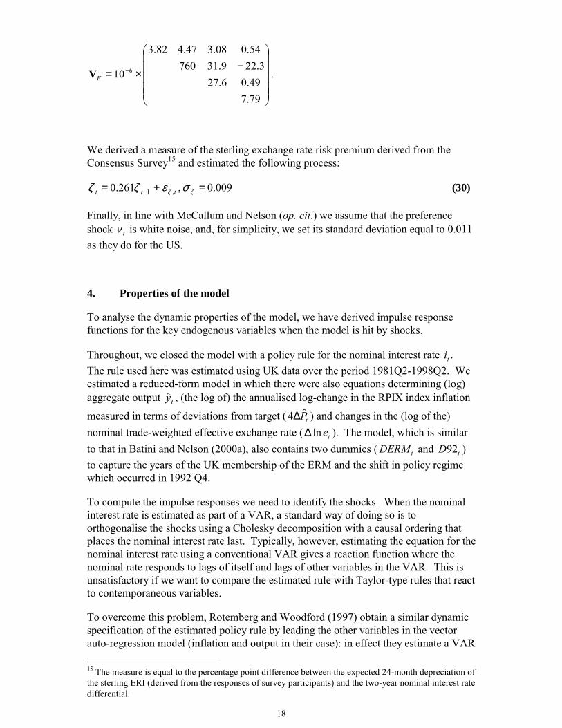
We derived a measure of the sterling exchange rate risk premium derived from theConsensus Survey15 and estimated the following process:

009.0 ,261.0 ,1 =+= − ζζ σεζζ ttt (30)

Finally, in line with McCallum and Nelson (op. cit.) we assume that the preferenceshock tν is white noise, and, for simplicity, we set its standard deviation equal to 0.011as they do for the US.

4. Properties of the model

To analyse the dynamic properties of the model, we have derived impulse responsefunctions for the key endogenous variables when the model is hit by shocks.

Throughout, we closed the model with a policy rule for the nominal interest rate ti .The rule used here was estimated using UK data over the period 1981Q2-1998Q2. Weestimated a reduced-form model in which there were also equations determining (log)aggregate output ty , (the log of) the annualised log-change in the RPIX index inflation

measured in terms of deviations from target ( tP4∆ ) and changes in the (log of the)nominal trade-weighted effective exchange rate ( teln∆ ). The model, which is similarto that in Batini and Nelson (2000a), also contains two dummies ( tDERM and 92tD )to capture the years of the UK membership of the ERM and the shift in policy regimewhich occurred in 1992 Q4.

To compute the impulse responses we need to identify the shocks. When the nominalinterest rate is estimated as part of a VAR, a standard way of doing so is toorthogonalise the shocks using a Cholesky decomposition with a causal ordering thatplaces the nominal interest rate last. Typically, however, estimating the equation for thenominal interest rate using a conventional VAR gives a reaction function where thenominal rate responds to lags of itself and lags of other variables in the VAR. This isunsatisfactory if we want to compare the estimated rule with Taylor-type rules that reactto contemporaneous variables.

To overcome this problem, Rotemberg and Woodford (1997) obtain a similar dynamicspecification of the estimated policy rule by leading the other variables in the vectorauto-regression model (inflation and output in their case): in effect they estimate a VAR 15 The measure is equal to the percentage point difference between the expected 24-month depreciation ofthe sterling ERI (derived from the responses of survey participants) and the two-year nominal interest ratedifferential.

19

with a vector of endogenous variables equal to [ ti4 , 14 +∆ tP , 1 +ty ]. Even if it gives an

estimated equation for the interest rate that responds to contemporaneous realisations ofoutput and inflation, as we want, their approach may be undesirable. It, in fact, impliesvery restricted dynamic specifications for the other two variables in the model, wherethe leads of inflation and output depend only on lags of the interest rate and not also onthe level of the interest rate at time t.

For this reason, following the methodology in Ericsson, Hendry and Mizon (1998), were-parameterised the system Qt = [ ti , tP4∆ , ty , teln∆ ] as the linear conditional and

marginal models ti = f ( tP4∆ , ty , teln∆ , 1−tQ ) and ( tP4∆ , teln∆ , ty ) = ( 1−tQ , χ), whereχ is the vector of estimated parameters. In effect, this orthogonalises the shocks, so thatthe nominal interest rate is not affected by time-t changes in the other variables.However, contrary to a standard VAR approach, this method allows us to derive anestimated equation for the nominal interest rate in which ti depends oncontemporaneous values of inflation, output and changes in the exchange rate, ratherthan on lags of those variables. The estimated coefficients are available on request. Forconvenience, we reproduce here the estimate of the nominal interest rate equation,which we interpret as being the monetary policy reaction function over that period:

tittttttt DDERMeyPici ,6543211 924ln444 εκκκκκκ +++∆++∆++= − (31)

where ti4 is the annualised interbank lending rate, and ti ,ε are the equations estimatedresiduals. The estimated coefficients (standard errors in parenthesis) are:

c = 0.0423, κ1 = 0.605, κ2 = 0.406, κ3 = 0.184, κ4 = − 0.065 ,

(0.008) (0.074) (----) (0.039) (0.027)

κ5 = − 0.014, κ6 = − 0.015,

(0.003) (0.004)

with SE = 0.00821.

To ensure that the log-run nominal interest rate response to inflation is larger than 1, werestrict )1/( 12 κκ − =1.01. For this reason, no standard error is reported for thatcoefficient. The LR test of over-identifying restrictions cannot reject the null impliedby this restriction [χ2(1)=0.5032, p -value = 0.4781].

Since the endogenous variables in the model feature as deviations from their respectivelong-run values or enter as first-differences they are comparable to variables inthe log-linearised first-order approximation version of the model.

20

Figure 1: Impulse responses following a 100 basis point monetary policy shock

-0.4

-0.3

-0.2

-0.1

0

0.1

1 3 5 7 9 11 13 15 17 19 21

Panel 1: Output Response

Quarter

-0.4

-0.2

0

0.2

0.4

0.6

1 3 5 7 9 11 13 15 17 19 21

Panel 2: Inflation Response

Quarter

-0.5

0

0.5

1

1.5

1 3 5 7 9 11 13 15 17 19 21

Panel 3: Nominal Interest Rate Response

Quarter

Figure 1 shows output, (four-quarter) inflation and the nominal interest rate impulseresponse functions to a unit start shock to the monetary policy rule (31) over 20 periods(calendar quarters). The solid line depicts the analytical models responses and thedashed line gives the estimated models responses.

The responses of both the empirical and the theoretical model broadly agree withconventional wisdom: following a temporary rise in the interest rate, output declines,but ultimately reverts to base; and inflation also falls. Our empirical model exhibits noprice puzzle (i.e. the finding in many empirically estimated models a rise in the nominalinterest rate is associated with a rise rather than a fall in the rate of inflation in theperiods immediately after the rise). However, we expect there to be rather wide errorbands around the empirical models impulse responses (not shown here) indicating that

21

these effects cannot be estimated with great precision, particularly those on inflation.So, the comparison of the two sets of responses should not be taken too literally.

Panel 1 indicates that, in our analytical model, output falls on impact by around 0.25%,following an unanticipated 100 basis point rise in the nominal interest rate the sameorder of magnitude of that of the estimated model. The policy shock response in thedata is slightly more sluggish than that in the model and in the data, the trough in outputfollowing the shock occurs later than in our model. The speedier response of output inour model reflects the volatility of the net trade component of aggregate output in ourmodel. The consumption component of aggregate output is sluggish and humpshaped, which reflects the high value of the habit formation parameter (ξ). This resultaccords with the findings of Fuhrer (2000).

Panel 2 compares the RPIX inflation responses of the theoretical and empirical models.In our model inflation responds earlier and more intensely than the empirical model.There, inflation touches its nadir around ten quarters after the shock, and returnssmoothly back on track over a period of about two to three years. The differencebetween the two responses probably reflects the fact that our model, even accountingfor the built-in persistence, is still a forward-looking, jumpier model, whereas theestimated model is entirely backward looking.

Panel 3 depicts how the (nominal) interest rate responds. While it rises by a full 1% inthe estimated model, the nominal interest rate by slightly less in our model. There aretwo reasons why this happens. First, in our model, inflation expected at time t + 1 fallson impact one period after the shock; by contrast, in the estimated model, inflation isalmost unchanged in the first quarters after the shock. This implies that, in practice, thereal interest rate response is harsher on impact in our model than in the estimatedmodel. Second, inflation and output (the feedback variables in the estimated policyrule) are forward-looking in our model; thus the interest rate response will be moremuted than in the estimated model, inasmuch as those variables will themselves adjustpre-emptively to the shock.

A second way of evaluating the correspondence between UK data and our model is tocompare the dynamic cross-correlations of key variables from the data with those fromthe model.16 Figure 2 shows this comparison for (log deviations of) aggregate output(y), value added sectoral outputs ( Nvy , and Xvy , ), annual CPI inflation ( 4π ), thenominal interest rate (i) and the real exchange rate (q). In each of the thirty-six panels,the solid line illustrates the theoretical cross-correlation function and the dashed line thecross-correlation function from the data.

Figure 2 indicates that our model seems to account for the auto-correlations of the datato a reasonable extent (see charts on the diagonal). In particular, our model can in partreplicate the degree of persistence of inflation seen in the data, although this is mainlydriven by persistence in the exogenous shocks. The model is perhaps less successful atcapturing cross-correlations: for example, the dynamic relationship between the realexchange rate and some of the other variables in the panel.

16 For the model, the cross-correlations were computed using a variant of the Hansen-Sargent doublingalgorithm discussed in section 5.

22

Figure 2: Cross-correlations of selected endogenous variableskty − ktNvy −,, ktXvy −,, kt−,4π kti − ktq −

ty

-1

-0.5

0

0.5

1

0 5 10

-1

-0.5

0

0.5

1

0 5 10

-1

-0.5

0

0.5

1

0 5 10

-1

-0.5

0

0.5

1

0 5 10

-1

-0.5

0

0.5

1

0 5 10

-1

-0.5

0

0.5

1

0 5 10

tNvy ,,

-1

-0.5

0

0.5

1

0 5 10

-1

-0.5

0

0.5

1

0 5 10

-1

-0.5

0

0.5

1

0 5 10

-1

-0.5

0

0.5

1

0 5 10

-1

-0.5

0

0.5

1

0 5 10

-1

-0.5

0

0.5

1

0 5 10

tXvy ,,

-1

-0.5

0

0.5

1

0 5 10

-1

-0.5

0

0.5

1

0 5 10

-1

-0.5

0

0.5

1

0 5 10

-1

-0.5

0

0.5

1

0 5 10

-1

-0.5

0

0.5

1

0 5 10

-1

-0.5

0

0.5

1

0 5 10

t.4π

-1

-0.5

0

0.5

1

0 5 10

-1

-0.5

0

0.5

1

0 5 10

-1

-0.5

0

0.5

1

0 5 10

-1

-0.5

0

0.5

1

0 5 10

-1

-0.5

0

0.5

1

0 5 10

-1

-0.5

0

0.5

1

0 5 10

ti

-1

-0.5

0

0.5

1

0 5 10

-1

-0.5

0

0.5

1

0 5 10

-1

-0.5

0

0.5

1

0 5 10

-1

-0.5

0

0.5

1

1.5

0 5 10

-1

-0.5

0

0.5

1

0 5 10

-1

-0.5

0

0.5

1

0 5 10

tq

-1

-0.5

0

0.5

1

0 5 10

-1

-0.5

0

0.5

1

0 5 10

-1

-0.5

0

0.5

1

0 5 10

-1

-0.5

0

0.5

1

0 5 10

-1

-0.5

0

0.5

1

0 5 10

-1

-0.5

0

0.5

1

0 5 10

5. Results: a comparison of alternative simple rules

In this section we present results from the model when it is closed with alternativemonetary policy rules. In what follows we assume that deviations of the nominalinterest rate from base are a linear function of deviations of endogenous variables(current, lagged or expected) from base. So we consider rules of the form,

tt Rgi = , ttg z⊆ . (32)

where g is the set of feedback variables in the rule and R is a row vector ofcoefficients.17 A simple rule therefore consists of two components, the vector offeedback variables, g, and the vector of coefficients, R. We define generic classes ofrules by the g vector, that is, by the set of variables on which they feed back. To carryout the comparison, for each rule we consider two kinds of coefficients vectors, R.

First, we look at the rules in their original specification. In this case, the vector ofcoefficients, R, is that suggested for those rules. For example, the first group of rulesincludes a Taylor rule with the original coefficients advocated by Taylor (1993a). We

17 Note that by using lag and lead identities within the model, the set of variables that could be includedin the rule is large. For example, for the inflation forecast based rule considered below, we includeconditional expectations of inflation up to five quarters ahead.

23

call these rules non-optimised because their coefficients are not set optimally for ourmodel.

Second, we consider simple optimised rules. In this case, the R vectors are those thatminimise the policymakers loss function, 1L , for each rule. In both cases (non-optimised and optimised rules), the specification of the rules is the one originallysuggested for those rules, i.e. the set of feedback variables g corresponds to the setinitially proposed by the rules first advocate.18 By contrast, as anticipated, in ourfamily of open economy simple rules, the vectors of feedbacks g vary relative to thevectors implied existing rules to better account for the exchange rate channel ofmonetary transmission.

As a measure of loss, 1L , we choose a standard quadratic loss function in asymptoticvariances of inflation deviations from target and output deviations from potential. Thisis often used as a metric for capturing policymakers preferences in studies that attemptto evaluate the performance of alternative policy rules [see Taylor (1999)].Algebraically, 1L can be written as:

)4()()4(),,(1 iAVarwyAVarwAVarwiyL iy ∆++= ππ π , (33)

which is a linear combination of the asymptotic variances (AVar) of annualisedinflation and output, and the change in the (annualised) nominal interest rate. FollowingBatini and Nelson (2000a) we set 1== ywwπ .

The inclusion of a term in the variability of the nominal interest rate is designed toaddress the fact that optimised coefficients for simple rules often imply very aggressivepolicy responses. In practice, this would lead to large movements in the policyinstrument. Casual empiricism suggests that policymakers prefer stability in theinstrument, which implies that nominal interest rate variability should be included inthe loss function.19 Perhaps more importantly, when taken literally, aggressive policyrules often imply that policymakers should set a negative nominal interest rate, despitethe general presumption that nominal rates cannot fall below zero. (See McCallum(2000) and Goodfriend (1999).) This issue is discussed in Williams (1999).

Including a term in the loss function is one way to ensure that rules with optimisedcoefficients do not imply that there is a high probability that the zero bound on thenominal interest rate is violated. The choice of the weight iw depends on the modelbeing used. Following Rudebusch and Svensson (1999), Batini and Nelson (2000a) set

5.0=iw . We set 25.0=iw which ensures that there is a relatively low probability ofviolating the zero bound for the optimised rules we consider. We discuss this furtherbelow.

Turning to the vector of optimised coefficients ( R~ ), this is chosen as follows:

18 For example an output gap and an inflation gap expressed in terms of deviations of actual inflationfrom its target or equilibrium value for the Taylor (1993) rule; and an expected inflation gap expressed in terms of deviations of future expected inflation from an inflation target and an interestrate smoothing term for the inflation forecast based rule.19 The fact that the interest rate smoothing term in the estimated rule equation (31) is high andsignificant, suggests that historically - interest rates have not responded aggressively in the UK.

24

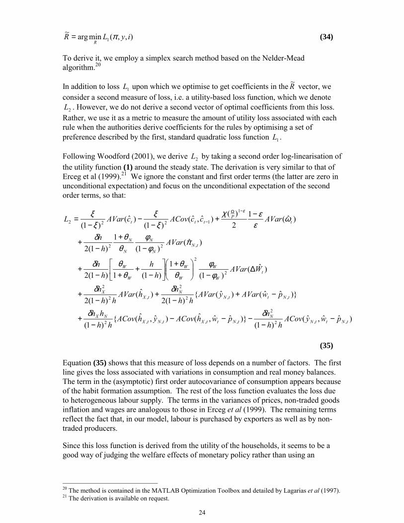
),,(minarg~1 iyLR

Rπ= (34)

To derive it, we employ a simplex search method based on the Nelder-Meadalgorithm.20

In addition to loss 1L upon which we optimise to get coefficients in the R~ vector, weconsider a second measure of loss, i.e. a utility-based loss function, which we denote

2L . However, we do not derive a second vector of optimal coefficients from this loss.Rather, we use it as a metric to measure the amount of utility loss associated with eachrule when the authorities derive coefficients for the rules by optimising a set ofpreference described by the first, standard quadratic loss function 1L .

Following Woodford (2001), we derive 2L by taking a second order log-linearisation ofthe utility function (1) around the steady state. The derivation is very similar to that ofErceg et al (1999).21 We ignore the constant and first order terms (the latter are zero inunconditional expectation) and focus on the unconditional expectation of the secondorder terms, so that:

),()1(

),(),()1(

)()()1(2

)()1(2

)()1(

1)1(1)1(2

)()1(

1)1(2

)(12)(

),()1(

)()1(

,,2

2

,,,,2

,,2

2

,2

2

2

2

,22

1

1222

tNttNN

tNttXtNtXNX

tNttNN

tXX

tW

W

W

W

W

W

tNN

N

N

N

tP

ttt

pwyACovhh

hpwhACovyhACov

hhhh

pwAVaryAVarhh

hhAVarhh

h

WAVarh

hh

h

AVarh

h

AVarccACovcAVarL

−−

−−−−

+

−+−

+−

+

∆−

+

−+

+−+

−+

−+

−+−

−−

=−Ω

−

δδ

δδ

φφ

θθ

θθδ

πφ

φθ

θδ

ωε

εχξ

ξξ

ξ ε

(35)

Equation (35) shows that this measure of loss depends on a number of factors. The firstline gives the loss associated with variations in consumption and real money balances.The term in the (asymptotic) first order autocovariance of consumption appears becauseof the habit formation assumption. The rest of the loss function evaluates the loss dueto heterogeneous labour supply. The terms in the variances of prices, non-traded goodsinflation and wages are analogous to those in Erceg et al (1999). The remaining termsreflect the fact that, in our model, labour is purchased by exporters as well as by non-traded producers.

Since this loss function is derived from the utility of the households, it seems to be agood way of judging the welfare effects of monetary policy rather than using an

20 The method is contained in the MATLAB Optimization Toolbox and detailed by Lagarias et al (1997).21 The derivation is available on request.

25

arbitrary loss function such as 1L as has been common in this literature.22

However, it is not necessarily ideal as it requires us to make some judgements abouthow to measure welfare in a model with heterogeneous households.

Finally, to obtain the asymptotic variances in equations (33) and (35), we first define avector ]x [ ′′′= ttt zn and use (24) and (25) to write the solution of our model as:

ttt RnRn υ)()( 1 Φ+Γ= − (36)

where the coefficients in the Γ and Φ matrices potentially depend on the rulecoefficients, R. The asymptotic variance of the state vector, n, is given by:

∞

=

Γ′Φ′ΦΩΓ=0j

jjV (37)

where Ω is the covariance matrix of the shocks, υ. We then compute V by the doublingalgorithm of Hansen and Sargent (1998), given the covariance matrix, Ω, calibrated insection 3. The asymptotic variance of any endogenous variable is given by the relevantelement of V.23

5.1 A battery of rules

We evaluate the relative performance of the following classes of rules:

(i) the estimated policy rule (see section 4);

(ii) a Taylor rule;

(iii) an inflation-forecast based (IFB) rule;

(iv) a naïve MCI-based rule;

(v) Balls (1999) rule;

(vi) a family of alternative open-economy rules.

This battery of rules encompasses the mainstream of the literature on simple policyrules for both closed and open economies, but adds a series of new simple rules thatslightly modify existing rules in the attempt to better suit monetary policy in openeconomies [(vi)]. The estimated rule enables us to assess the remaining rules vis-à-vishistory, and to infer whether, using these other rules, it may have been possible to dobetter than historically. We discuss the remaining classes of rules in turn.

22 Note that, because we characterise the economy using a log-linear approximation, there is no clearadvantage to evaluating an exact utility function; see Woodford (2001, p5).23 This approach is also used by Williams (1999).

26

The Taylor rule

This section considers rules of the following form:

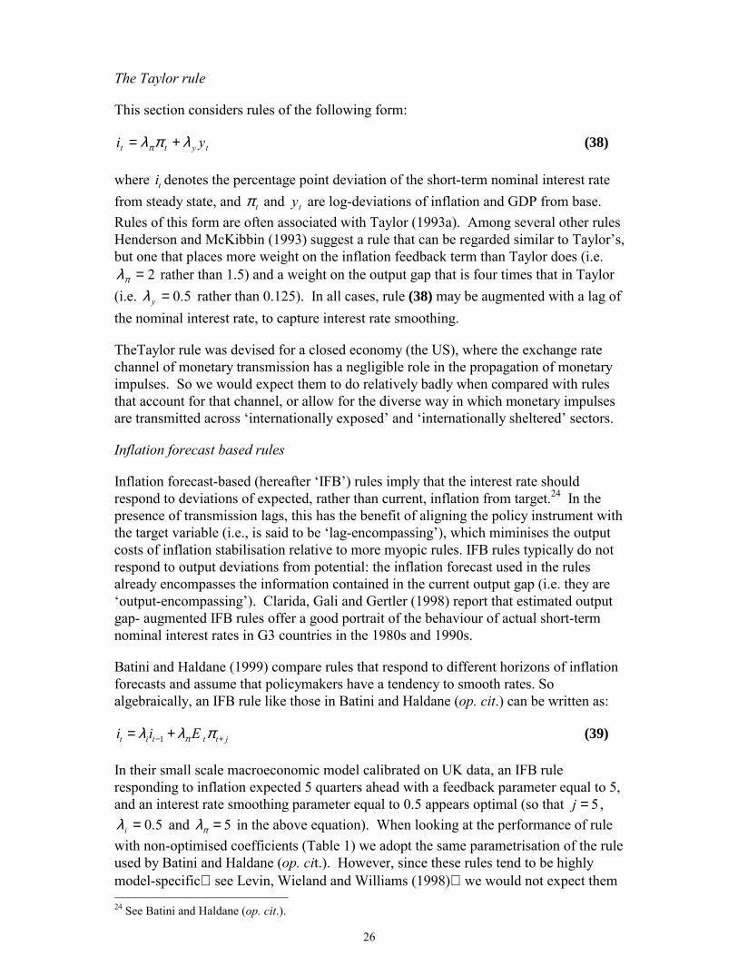
tytt yi λπλπ += (38)

where ti denotes the percentage point deviation of the short-term nominal interest ratefrom steady state, and tπ and ty are log-deviations of inflation and GDP from base.Rules of this form are often associated with Taylor (1993a). Among several other rulesHenderson and McKibbin (1993) suggest a rule that can be regarded similar to Taylors,but one that places more weight on the inflation feedback term than Taylor does (i.e.

2=πλ rather than 1.5) and a weight on the output gap that is four times that in Taylor(i.e. 5.0=yλ rather than 0.125). In all cases, rule (38) may be augmented with a lag ofthe nominal interest rate, to capture interest rate smoothing.

TheTaylor rule was devised for a closed economy (the US), where the exchange ratechannel of monetary transmission has a negligible role in the propagation of monetaryimpulses. So we would expect them to do relatively badly when compared with rulesthat account for that channel, or allow for the diverse way in which monetary impulsesare transmitted across internationally exposed and internationally sheltered sectors.

Inflation forecast based rules

Inflation forecast-based (hereafter IFB) rules imply that the interest rate shouldrespond to deviations of expected, rather than current, inflation from target.24 In thepresence of transmission lags, this has the benefit of aligning the policy instrument withthe target variable (i.e., is said to be lag-encompassing), which miminises the outputcosts of inflation stabilisation relative to more myopic rules. IFB rules typically do notrespond to output deviations from potential: the inflation forecast used in the rulesalready encompasses the information contained in the current output gap (i.e. they areoutput-encompassing). Clarida, Gali and Gertler (1998) report that estimated outputgap- augmented IFB rules offer a good portrait of the behaviour of actual short-termnominal interest rates in G3 countries in the 1980s and 1990s.

Batini and Haldane (1999) compare rules that respond to different horizons of inflationforecasts and assume that policymakers have a tendency to smooth rates. Soalgebraically, an IFB rule like those in Batini and Haldane (op. cit.) can be written as:

1t i t t t ji i Eπλ λ π− += + (39)

In their small scale macroeconomic model calibrated on UK data, an IFB ruleresponding to inflation expected 5 quarters ahead with a feedback parameter equal to 5,and an interest rate smoothing parameter equal to 0.5 appears optimal (so that 5j = ,

5.0=iλ and 5πλ = in the above equation). When looking at the performance of rulewith non-optimised coefficients (Table 1) we adopt the same parametrisation of the ruleused by Batini and Haldane (op. cit.). However, since these rules tend to be highlymodel-specific see Levin, Wieland and Williams (1998) we would not expect them 24 See Batini and Haldane (op. cit.).

27

to do well in our model for the same choice of horizon and feedback parameters thatwas efficient in Batini and Haldane (op. cit.). Indeed, the low degree of inflationpersistence in our model suggests that a shorter horizon is probably more adequate.Hence, in the experiments using optimised coefficients we also select the horizonoptimally, treating the horizon as a policy parameter as in Batini and Haldane (1999).

The naïve MCI-based rule

A Monetary Condition Index (MCI) is a weighted average of the domestic interest rateand the (log) exchange rate.25 A MCI can be expressed in real or nominal terms.Because it has the potential to quantify the degree of tightness (ease) that both theinterest rate and the exchange rate exert on the economy, MCIs are often used tomeasure the stance of monetary policy in an open economy.

A naïve simple rule based on a MCI could then be one that entails adjusting thenominal interest rate to ensure that real monetary conditions are unchanged over time:

t t ti qπ µ= − (40)

where qt is the real exchange rate and µ is the MCI weight.26 Setting µ =1/3 a valueconsistent with the weights used by the Bank of Canada to construct an MCI impliesthat a 3% appreciation in the real exchange rate is equivalent to a 100 basis pointsincrease in the real interest rate.27

In practice, MCIs have been criticised on both empirical and theoretical grounds.28

One conceptual shortcoming of a MCI, when used as an operating target, is thatdifferent types of shocks have different implications for monetary policy. Byconstruction, a MCI obscures the identification of exchange rate shocks because thisrequires focusing on movements in the exchange rate and interest rates in isolation,rather than aggregated together (see King (1997)). This shortcoming carries over to anyMCI-based rule that recommends a level for the interest rate conditioning on theexisting level of the exchange rate, when the latter can change for shocks that thecentral bank may not wish to respond to. For this reason, we would expect theperformance of MCI-based rules to be shock-specific, doing poorly in the face ofshocks that affect the exchange rate but do not ask for a compensating change ininterest rates (e.g. shocks to the real exchange rate). 25 See Batini and Turnbull (2000) for a thorough discussion of MCIs, their potential flaws and theirpossible uses for the UK.26 We do not consider nominal MCIs as they are likely to perform poorly in our model. The reason is thatthe level of the nominal exchange rate can shift permanently following a transitory nominal shock. Thissuggests that a simple nominal MCI rule could lead to instability.27 In practice, the actual MCI may be compared with a desired MCI level, MCI*, say. MCI* is the levelof monetary conditions compatible with the inflation target and non-inflationary economic growth. In thissense, the desired MCI can be viewed as an open economy extension of Blinders (1998) concept of aneutral rate, an interest rate at which the monetary stance is neither dampening nor stimulatingeconomic activity. In a closed economy, the monetary authority will want the actual nominal rate todepart from its neutral level, whenever the economy is out of equilibrium and vice-versa. In an openeconomy, the monetary authority may want the actual MCI to deviate from MCI* for the same reason.But it is not entirely clear from the existing literature how MCI-based rules expressed in terms ofdeviations of actual from desired should be constructed. Basically this is because to do so requiresknowledge of how desired monetary conditions will evolve.28 See, among others, Ericsson et al (1997).

28

Balls (1999) rule

Less naïve specifications of a rule which use a monetary conditions index as a policyinstrument may potentially perform better. Ball (1999) proposes a rule of this kindwhere policymakers alter a combination of interest and exchange rates in response todeviations of (an exchange-rate-adjusted or long-run measure of) inflation from targetand output from potential. When the rule is re-arranged so that only the nominalinterest rate features on the left-hand side of the equation, this rule indeed resembles aTaylor rule with added real exchange rate (contemporaneous and lagged) terms:

121 −+++= tqtqttyt qqyi λλπλλ π (41)

In this sense, Balls rule is an open economy rule because responding also to theexchange rate, it expands parsimoniously upon closed-economy rules to account foropenness of the economy. So we would imagine that it outperforms closed-economycounterparts when utilised to control our open-economy model. This rule is in factoptimal in Balls (1999) model, a model that contains only three states (inflation, outputand the exchange rate). The coefficients that Ball suggests, conditioning on hisdynamic constraints, are: 93.1=yλ , 51.2=πλ , 43.01 −=qλ and 3.02 =qλ . These arethe coefficients we use in the experiments with non-optimised coefficients. As we willsee below, three rules in our family of open economy rules can be consideredextensions of Balls rule.

A family of alternative open economy simple rules

Finally, we turn to our set of alternative open economy rules. As anticipated, theserules are designed for an economy that is open.

Ideally, following Ball (1999), we want these rules to do two things. First, alongsidethe standard output gap channel, the rules should also exploit the exchange rate channelof monetary transmission. This should make policy more effective by letting sectors inthe economy that are affected unevenly by the two major channels of transmissionadjust in the most efficient way following a shock. Second, they should do so byaugmenting its closed-economy counterpart rules specifications (e.g., Taylor andHenderson and McKibbin) in a parsimonious way. This is because, both on credibilityand monitorability grounds, there is a clear merit in having a rule that is simple tocompute that is a rule that does not introduce any extra uncertainty in themeasurement of its arguments and that can be easily understood by the public.

For this purpose we consider four different rules, which account for the openness of theeconomy in various ways. Three of these can be considered variants of Balls (1999)rule. More specifically, the first variant (OE2) adds to the standard feedback terms inBalls rule a term responding to the balance of trade. The second variant (OE3)replaces aggregate output with output gaps in the two sectors; this takes explicitaccount of the fact that components of GDP differ in their international exposure. Andthe third variant (OE4) has the interest rate responding to the same variables as in Ball(1999), but imposes a restriction on the contemporaneous and lagged real exchange rateterms, so that their coefficients are equal and opposite. In practice, this implies that thepolicymakers respond to time-t changes in the real exchange rate rather than levels of it.The fourth and final rule in the family (OE1) instead, is a modification of the inflation

29

forecast based rule of Batini and Haldane (1999), which adds to that an explicitresponse to the real exchange rate (again contemporaneous and lagged, unrestricted).In principle, an IFB rule already accounts for the exchange rate channel of monetarytransmission, inasmuch as this underlies the equations that inform the forecast forinflation. So evaluating this rules enables us to understand whether incorporating aseparate exchange rate term in an IFB rule provides information over and above thatalready contained in the inflation forecast. 29

As with the IFB and Balls rules, we expect rules in this family (especially rules OE2,OE3 and OE4) to do better on average than their closed-economy counterparts. This isbecause they take explicit account of the fact that in an open economy there aremultiple channels of monetary transmission that can be simultaneously exploited in aneffective way. However, since the IFB rule already exploits the exchange rate channelof policy transmission, accounting for this channel explicitly may not add much to thestabilisation properties of this rule. In general, other things being equal, and like withthe IFB rule and Balls rule, we expect at least some of the OE rules to reduce thedisparities in the costs of adjustment faced by the two sectors in the economy, relativeto the closed economy simple rules case. Lastly, note that under optimisation these rulesmay also do better than the Taylor and the IFB rules because they typically react tomore state variables. We will discuss this issue in more detail below.

5.2 Results

Table 1 below contains values of the two loss functions ( 1L and 2L ) and asymptoticsecond order moments of inflation, output, the nominal interest rate, sectoral outputsand the real exchange rate. These are reported for the estimated rule, the Taylor (andHenderson and McKibbin) rule(s), the IFB rule, the naïve MCI-based rule and Ballsrule with the original weights under our model specification. Table 2, in turn, reportsanalogous statistics for these rules (excluding the estimated rule) and for the OE1, OE2,OE3 and OE4 rules when coefficients are set optimally. This table also reportscorresponding optimised rules coefficients. Finally, Table 3 offers a test for relativerobustness, by showing the same statistics for each rule when the model is hit byindividual shocks rather than by a combination of shocks.

5.2.1 Results under an all shocks scenario

Table 1 suggests that, when coefficients are not optimised and all the shocks in themodel are operative, the best performing rule according to loss function 1L is,surprisingly, the naïve MCI-based rule, which ensures the lowest volatility of the realexchange rate and of exports. This in turn gives better inflation control than Taylor andHenderson and McKibbin rules. Among these, the latter is more successful than theTaylor rule at stabilising both output and inflation a consequence of its strongerfeedback coefficients.

The estimated rule ranks fourth. Thanks to its term for interest rate smoothing, this ruleresponds gradually to inflationary pressures, and thus minimises interest rate and outputvolatility compared to Taylor/Henderson-McKibbin rules. On the other hand, thismakes the estimated rule less successful at stabilising inflation than those rules. When 29 See also Batini and Nelson (2000b) for a comprehensive study of this issue using a small-scalestructural model of the UK economy.

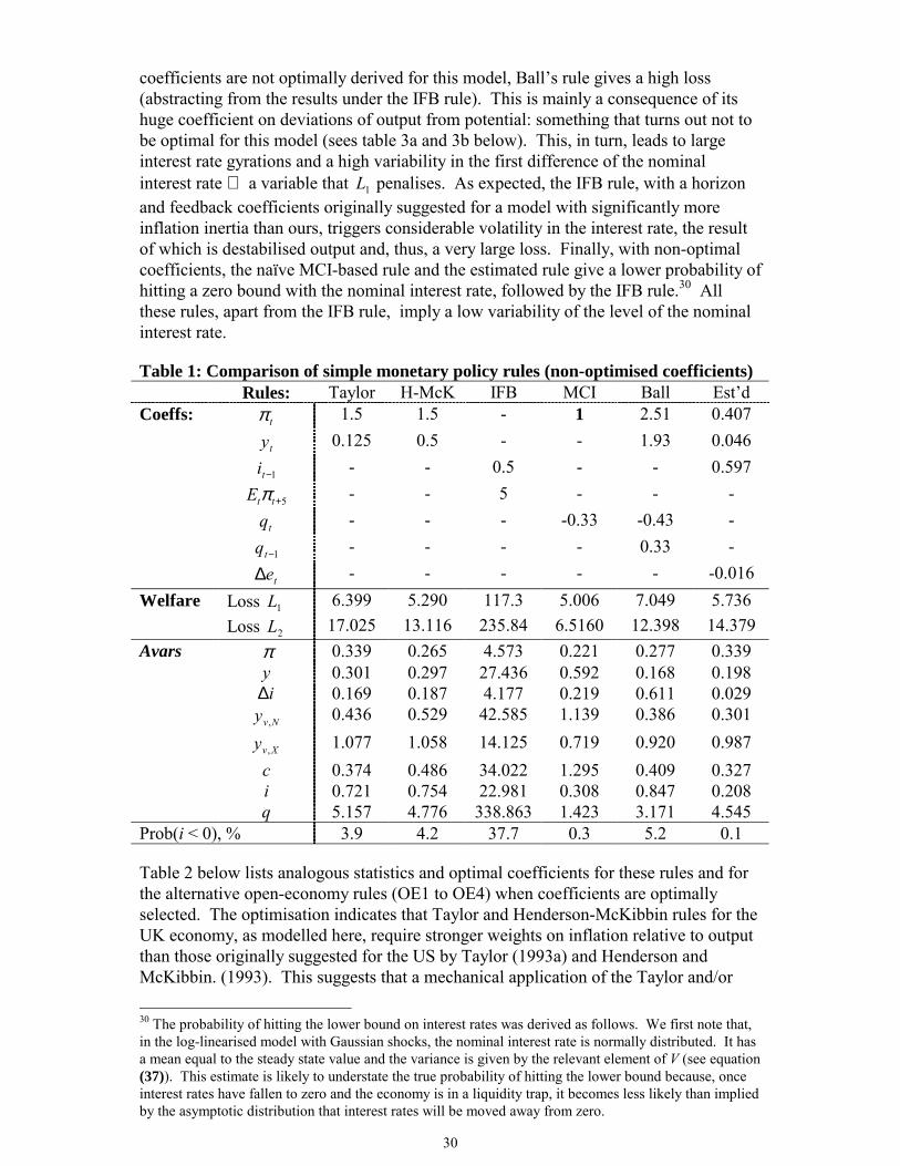
30

coefficients are not optimally derived for this model, Balls rule gives a high loss(abstracting from the results under the IFB rule). This is mainly a consequence of itshuge coefficient on deviations of output from potential: something that turns out not tobe optimal for this model (sees table 3a and 3b below). This, in turn, leads to largeinterest rate gyrations and a high variability in the first difference of the nominalinterest rate a variable that 1L penalises. As expected, the IFB rule, with a horizonand feedback coefficients originally suggested for a model with significantly moreinflation inertia than ours, triggers considerable volatility in the interest rate, the resultof which is destabilised output and, thus, a very large loss. Finally, with non-optimalcoefficients, the naïve MCI-based rule and the estimated rule give a lower probability ofhitting a zero bound with the nominal interest rate, followed by the IFB rule.30 Allthese rules, apart from the IFB rule, imply a low variability of the level of the nominalinterest rate.

Table 1: Comparison of simple monetary policy rules (non-optimised coefficients)Rules: Taylor H-McK IFB MCI Ball Estd

Coeffs: tπ 1.5 1.5 - 1 2.51 0.407

ty 0.125 0.5 - - 1.93 0.046

1−ti - - 0.5 - - 0.597

5t tE π + - - 5 - - -

tq - - - -0.33 -0.43 -

1−tq - - - - 0.33 -

te∆ - - - - - -0.016Welfare Loss 1L 6.399 5.290 117.3 5.006 7.049 5.736

Loss 2L 17.025 13.116 235.84 6.5160 12.398 14.379Avars π 0.339 0.265 4.573 0.221 0.277 0.339

y 0.301 0.297 27.436 0.592 0.168 0.198i∆ 0.169 0.187 4.177 0.219 0.611 0.029Nvy , 0.436 0.529 42.585 1.139 0.386 0.301

Xvy , 1.077 1.058 14.125 0.719 0.920 0.987c 0.374 0.486 34.022 1.295 0.409 0.327i 0.721 0.754 22.981 0.308 0.847 0.208q 5.157 4.776 338.863 1.423 3.171 4.545

Prob(i < 0), % 3.9 4.2 37.7 0.3 5.2 0.1

Table 2 below lists analogous statistics and optimal coefficients for these rules and forthe alternative open-economy rules (OE1 to OE4) when coefficients are optimallyselected. The optimisation indicates that Taylor and Henderson-McKibbin rules for theUK economy, as modelled here, require stronger weights on inflation relative to outputthan those originally suggested for the US by Taylor (1993a) and Henderson andMcKibbin. (1993). This suggests that a mechanical application of the Taylor and/or 30 The probability of hitting the lower bound on interest rates was derived as follows. We first note that,in the log-linearised model with Gaussian shocks, the nominal interest rate is normally distributed. It hasa mean equal to the steady state value and the variance is given by the relevant element of V (see equation(37)). This estimate is likely to understate the true probability of hitting the lower bound because, onceinterest rates have fallen to zero and the economy is in a liquidity trap, it becomes less likely than impliedby the asymptotic distribution that interest rates will be moved away from zero.

31

Henderson and McKibbin rules in the UK context with coefficients designed for the USis not ideal. Moreover, our model seems to favour a stronger weight on inflationrelative to output, even when the policymakers preferences are symmetric betweeninflation and output stabilisation.

Similarly, for our model economy, the optimal coefficient for the MCI-based rule issmaller than one third the value commonly used in the MCI literature suggestingthat a greater weight than that used in practice should be placed on interest rates vis-à-vis the exchange rate when altering monetary conditions.

Table 2: Comparison of simple monetary policy rules (optimised coefficients)Rules Taylor/

H-McKIFB MCI Ball OE1 OE2 OE3 OE4

Coeffs: tπ 5.94 - 1 5.117 - 4.111 5.193 5.869

ty 0.23 - - -0.036 - 0.053 - 0.228

1−ti - 0.913 - - 0.947 - - -

1+ttE π - 0.808 - - 1.093 - - -

tq - - -0.220

-0.110 -0.015

-0.071 -0.064

-

1−tq - - - -0.047 -0.024

-0.054 -0.039

-

tNvy ,, - - - - - - -0.035

-

tXvy ,, - - - - - - 0.148 -

tq∆ - - - - - - - -0.029

tBT - - - - - 6.476 - -Welfare Loss 1L 2.68 2.08 4.82 2.59 1.987 2.548 2.580 2.654

Loss 2L 5.9151 3.219 6.927 5.000 3.020 4.587 5.103 5.916Avars π 0.029 0.029 0.234 0.031 0.029 0.033 0.030 0.029

y 1.608 1.540 0.449 1.489 1.425 1.452 1.522 1.614i∆ 0.151 0.018 0.156 0.152 0.023 0.144 0.147 0.145Nvy , 2.958 2.832 0.859 2.742 2.646 2.708 2.799 2.972

Xvy , 1.178 1.137 0.768 1.120 1.078 1.105 1.108 1.172c 2.679 2.668 1.001 2.525 2.525 2.517 2.583 2.692i 0.613 0.170 0.287 0.582 0.198 0.544 0.581 0.607q 6.431 5.332 1.923 5.503 4.592 5.257 5.512 6.327

Prob(i < 0), % 2.8 0.0 0.3 2.5 0.0 2.1 2.5 2.7

Looking at the stabilisation properties of each rule, the first thing to notice is thatTaylor/HendersonMcKibbin, IFB and Balls rules perform much better than theircounterparts with non-optimised coefficients. This is not true of the naïve MCI-basedrule, since its performance is almost unaffected by the optimisation of its (unique)coefficient, making it the worse rule in the set. Indeed, when coefficients areoptimised, rules in the Taylor/Henderson-McKibbin class now outperform the naïveMCI-based rule by ensuring lower inflation volatility.

Second, with optimally chosen horizon and feedback coefficients (both significantlyreduced from the non-optimal case), the IFB rule performs extraordinarily well. When

32

coefficients are optimal, the IFB rule appears to be extremely successful at minimisinginflation volatility for a level of output volatility that is now comparable, if not lower,than that of other rules in the table. This is a consequence of the fact that, under thisrule, the interest rate now moves optimally and solely to correct low-frequency changesin inflation. (The asymptotic standard deviation of changes in the nominal interest ratefor this rule is, in fact, around a tenth of that under all other rules if we exclude the OE1rule, a modification of the IFB.) This result is in line with the findings in Batini andHaldane (1999) based on a small-scale, open economy model of the UK economy.

Third, Balls rule provides a lower than average variability of output when compared toTaylor/Henderson-McKibbin and to the IFB rule. Relative to them, it also reduces thedisparity between output sector volatilities in the two sectors, other things being equal.However, it produces more interest rate, exchange rate and ultimately inflationvariability than the IFB rule because it reacts to current, rather than expected inflationand hence necessitates greater aggressiveness. This rule is, unsurprisingly, moreefficient than the simplistic MCI-based rule which does not react either to inflation noroutput, and which thus is unsuited to cope with inflationary shocks that did notoriginate in a shock to the exchange rate.

Additional results emerge when we look at our family of open economy rules.

In general, it seems as if parsimonious modifications of either Balls or the IFB rule donot gain much in terms of inflation or output control. The reduction in the value of 1Lis indeed negligible and most certainly ascribable to the fact that rules in the OE familytypically react to more state variables. By construction, this gives them a performancebonus relative to non-OE rules. By the same logic, the opposite is true of rule OE4 a restricted version of Balls rule which hence does worse than Balls rule itself.

However, on the whole, rules OE2 (Ball plus response to balance of trade), OE3 (Ballwith separate response to sectoral outputs) and OE1 (IFB with additional exchange rateterms) do seem capable of reducing further the disparity between output sectorvolatilities in the two sectors, others things being equal.

When we look at each rule individually, the following emerges. In rules OE2 and OE3which feed back on the balance trade and on sectoral output gaps respectively,introducing extra terms has the effect of lowering slightly the response to exchange rateterms as the optimised Balls rule would imply in the absence of those terms. And inOE2, adding a feedback term on the trade balance inverts the sign on the output gapterm (which was, somewhat counterintuitively, negative in Balls optimised rule). Thisis possibly a consequence of the fact that when policymakers respond separately to thenet trade component of the aggregate output gap, policy no longer needs to give aprocyclical response to the output gap. The implications of these changes in existingcoefficients combined with the effect of new coefficients are that: (i) OE2 gives amarginally better control than Balls rule of output and interest rates, but a slightlyworse control of inflation; (ii) OE3 gives a marginally better control of inflation andinterest rates than Balls rule, but worsens slightly the control of output; and (iii) onlyOE2 ensures more symmetry than Balls rule in the adjustment of sectoral outputs aftera shock.

Adding separate exchange rate terms to the IFB rule (OE1) also moderately improvesits stabilisation properties. The rule now delivers a lower volatility of output than

33

without the exchange rate terms. Exchange rate volatility also falls. OE1 is in fact thebest rule in the table. Compared to non-OE rules, OE1 gives considerably lower output,exchange rate and interest rate variability than Taylor/Henderson-McKibbin rules andalso than Balls rule. If we abstract from the naïve-MCI that smooths the costs ofadjustment across sectors but does badly in term of inflation variability, OE1 producesthe minimum disparity between the volatility of the output gap in the two sectors. Notethat, thanks to their ability of minimising the volatility of the policy instrument, IFB andOE1 rules also give the lowest probability of hitting a zero bound with the nominalinterest rate. These results on the relative performance of the rules are confirmed byour second measure of loss, the utility-based loss function 2L . According to thismetric, households would be better off if policymakers followed an OE1 rule or an IFBrule with coefficients optimised over the objective function 1L , rather than other rulesthat we consider. The worse possible rule according to 2L is instead theTaylor/Henderson-McKibbin.

In summary:

• IFB rules appear to be efficient open economy rules because they capture allchannels of transmission. They outperform closed economy rules like Taylor andHenderson-McKibbin in terms of both output and interest rate control. But they alsoprove superior to Balls rule, which reacts to current, rather than expected inflation.This makes policy myopic rather than pre-emptive, and hence requires moreaggressive changes in the interest rate, which in turn affect the exchange rate andthereby inflation. For these reasons, IFB rules also help stabilise the economy in amore symmetric way, demanding less adjustment from the the internationallyexposed sector than that required by closed-economy rules which ignore differencesin adjustment across sectors;

• Modifications to these rules to include explicit feedbacks on the level of the realexchange rate (contemporaneous and lagged) improve the performance of theserules only marginally. But since they help reduce further the disparity in adjustmentbetween traded and exports sectors, they may be desirable if the authorities have aspecific preference for symmetry in adjustment, other things equal.

• Relative to other rules in the battery, IFB and exchange-rate-adjusted IFB (OE1)minimise the probability of hitting a zero bound with nominal interest rates, andthereby increase the chances of policy remaining operational under particularlysevere deflationary shocks;

• Balls rule and variants of it (notably OE2 which allows a response to disequilibriain the trade balance) are second-best options. Because they also account for theexchange rate channel of transmission, as expected they are significantly moreefficient than Taylor/Henderson-McKibbin rules in stabilising inflation and outputin our open economy model of the UK. In this respect they are indeed by farpreferable to naïve MCI-based rule, which gives more stable output outcomes at theprice of massive inflation variance (the loss associated with Balls rule is a sixth ofthe loss associated with the naïve MCI-based rule).

34

5.2.2 Robustness analysis to individual shocks

In order to provide more intuition about why certain rules perform better than others,we have re-assessed the performance of the rules assuming that the economy was hit byone type of shock at a time. In particular, we are looking to see which rules producesensible responses to each of the shocks and analyse whether or not the rules thatperform well do so because they are robust to many different shocks. In each case, thecoefficients in the rules are again those optimally derived for the all-shocks case(shown in Table 2), so this is a test of robustness of the exact rule specification.31

Results from this experiment are summarised in Tables 3a and 3b below.

The tables suggest that the OE1 (i.e. the modified IFB) rule and the IFB rule itself arestill the best rules under most shocks. The OE1 (and to some extent also the originalIFB) rule seems to perform particularly well in the face of shocks from overseas.However, both the OE1 and the IFB rules are outperformed by the OE4 (restricted Ball)rule and by their closed-economy counterparts under productivity shocks to theexports sector. (OE1 and IFB are also inferior to OE4 and Taylor/Henderson-McKibbin under a shock to non-traded goods sector productivity but this is less severethan in the case of a shock to productivity to the export sector). The reason why thishappens is that a shock to productivity in the export sector will affect both export pricesand output. Since export prices do not enter the calculation of CPI inflation, rules likeOE1 or IFB that respond only to consumer price inflation will not perform well becausethey fail to respond to the first round effects of this shock. This is in line with thegeneral intuition that a simple rule can be a good guide for policy in the face of some but not all shocks. Crucially, however, the IFB and the OE1 rules seems morerobust to different shocks than the naïve MCI-based rule or Balls rule. This isparticularly evident for overseas shocks (e.g. foreign interest rate shocks and shocks tothe risk premium), but also to shocks to the price of intermediate inputs and to shocksto world output and inflation. In the case of Balls rule, this is also true for shocks toproductivity to both the export sector and the non-traded goods sector.

A comparison of the losses associated with each shock in turn reveals that the mostcostly shock by far is that to intermediates prices. This is because this shock not onlyhas a higher variance than other shocks but it is also highly cross-correlated with otheroverseas shocks. In fact, intermediate prices are a large proportion of unit costs in bothsectors. For instance, since non-traded producers set prices as a mark up over unitcosts, changes in these prices feed directly through non traded price inflation. On theother hand, shocks to the export sector seem to be relatively unimportant given the sizeof this sector and the openness of the economy. This is because shocks to this sectorare largely absorbed by the price of exports which is not a component of CPI inflation.

Given that a shock to intermediate prices is the most costly of our shocks, we wouldideally wish to use a monetary policy rule that generated the appropriate response tothis shock. In particular, we know that optimal policy would want to absorb the first-round effects of this shock but would want to make sure that there was no long-runeffect on inflation. A standard rule that feeds back off current inflation may lead to

31 To perform this test, we have re-derived losses and asymptotic second moments of the variables ofinterest by setting the variances of the remaining shocks to zero.

35

policy that was too tight and cause a fall in output. By contrast, the IFB and OE1 rulesact to stabilise future inflation rather than current: exactly the policy response thatseems appropriate for this sort of shock.

The results of this section suggest that OE1 and IFB rules manage to dominate all otherrules in an all-shocks scenario because they are efficient at stabilising the economy inthe face of overseas shocks (among which are, notably, shocks to intermediate prices).

36

Table 3a: Comparison of simple monetary policy rules (individual shocks)Taylor/H-McK

IFB MCI Ball OE1 OE2 OE3 OE4

Non-traded productivity shockLoss 1L 0.0233 0.0240 0.0267 0.0277 0.0238 0.0268 0.0277 0.0233

Avars π 0.0000 0.0000 0.0005 0.0000 0.0000 0.0000 0.0001 0.0000

y 0.0226 0.0237 0.0188 0.0243 0.0233 0.0254 0.0235 0.0227i∆ 0.0000 0.0000 0.0001 0.0007 0.0000 0.0002 0.0008 0.0000

Nvy ,0.0046 0.0054 0.0007 0.0052 0.0048 0.0088 0.0042 0.0047

Xvy ,0.0117 0.0119 0.0100 0.0121 0.0118 0.0126 0.0118 0.0117

c 0.0017 0.0021 0.0000 0.0018 0.0017 0.0045 0.0012 0.0017i 0.0001 0.0001 0.0004 0.0005 0.0001 0.0004 0.0006 0.0001q 0.0036 0.0050 0.0001 0.0069 0.0045 0.0069 0.0060 0.0036

Export productivity shockLoss 1L 0.0492 0.0507 0.0487 0.0518 0.0505 0.0579 0.0562 0.0485

Avars π 0.0000 0.0000 0.0000 0.0000 0.0000 0.0003 0.0000 0.0000

y 0.0445 0.0507 0.0483 0.0517 0.0505 0.0359 0.0547 0.0445i∆ 0.0010 0.0000 0.0000 0.0000 0.0000 0.0044 0.0002 0.0008

Nvy ,0.0001 0.0004 0.0000 0.0005 0.0003 0.0013 0.0009 0.0001

Xvy ,0.0550 0.0507 0.0510 0.0507 0.0508 0.0615 0.0487 0.0549

c 0.0001 0.0001 0.0000 0.0002 0.0001 0.0015 0.0005 0.0001i 0.0005 0.0000 0.0000 0.0000 0.0000 0.0022 0.0001 0.0004q 0.0023 0.0002 0.0000 0.0003 0.0002 0.0146 0.0012 0.0022

FX risk premium shockLoss 1L 0.1013 0.0187 0.2486 0.1287 0.0146 0.1150 0.1204 0.0891

Avars π 0.0006 0.0009 0.0007 0.0004 0.0005 0.0004 0.0004 0.0007

y 0.0013 0.0019 0.0010 0.0007 0.0033 0.0008 0.0008 0.0015i∆ 0.0226 0.0006 0.0592 0.0305 0.0009 0.0269 0.0282 0.0190

Nvy ,0.0006 0.0001 0.0001 0.0004 0.0045 0.0003 0.0004 0.0008

Xvy ,0.0372 0.0483 0.0309 0.0300 0.0389 0.0316 0.0310 0.0363

c 0.0004 0.0002 0.0003 0.0004 0.0052 0.0004 0.0004 0.0004i 0.0219 0.0008 0.0440 0.0377 0.0023 0.0324 0.0347 0.0232q 0.9686 1.2620 0.8071 0.7787 1.0156 0.8226 0.8067 0.9445

Preference shockLoss 1L 0.1310 0.1253 0.1336 0.1275 0.1258 0.1347 0.1277 0.1281

Avars π 0.0001 0.0000 0.0001 0.0000 0.0000 0.0001 0.0000 0.0001

y 0.1121 0.1252 0.1324 0.1272 0.1257 0.1330 0.1274 0.1121i∆ 0.0044 0.0000 0.0000 0.0000 0.0000 0.0002 0.0000 0.0037

Nvy ,0.1718 0.1893 0.2000 0.1923 0.1900 0.2004 0.1926 0.1718

Xvy ,0.0004 0.0000 0.0000 0.0000 0.0000 0.0000 0.0000 0.0004

c 0.1867 0.2041 0.2148 0.2072 0.2048 0.2152 0.2074 0.1867i 0.0022 0.0000 0.0001 0.0000 0.0000 0.0001 0.0000 0.0019q 0.0117 0.0007 0.0000 0.0004 0.0006 0.0002 0.0004 0.0112

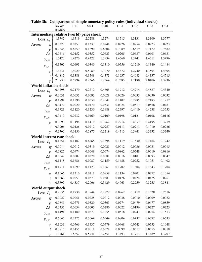
37

Table 3b: Comparison of simple monetary policy rules (individual shocks)Taylor/H-McK

IFB MCI Ball OE1 OE2 OE3 OE4

Intermediate relative (world) price shockLoss 1L 1.3742 1.1519 2.5288 1.3274 1.1515 1.3131 1.3100 1.3777

Avars π 0.0227 0.0253 0.1337 0.0248 0.0226 0.0254 0.0223 0.0223

y 0.7648 0.6859 0.1690 0.6804 0.7089 0.6519 0.7122 0.7682i∆ 0.0616 0.0152 0.0552 0.0623 0.0205 0.0637 0.0601 0.0631

Nvy ,1.5420 1.4270 0.4322 1.3934 1.4660 1.3441 1.4511 1.5496

Xvy ,0.1502 0.0693 0.0340 0.1310 0.0756 0.1210 0.1340 0.1484

c 1.4231 1.4029 0.5089 1.3070 1.4372 1.2740 1.3594 1.4305i 0.4815 0.1388 0.1548 0.4373 0.1637 0.4083 0.4337 0.4715q 2.3738 0.5994 0.2366 1.9364 0.7385 1.7180 2.0106 2.3236

World inflation shockLoss 1L 0.4298 0.2179 0.2712 0.4605 0.1912 0.4914 0.4887 0.4340

Avars π 0.0031 0.0032 0.0093 0.0028 0.0026 0.0035 0.0030 0.0032

y 0.1894 0.1590 0.0550 0.2042 0.1402 0.2285 0.2183 0.1912i∆ 0.0477 0.0020 0.0170 0.0531 0.0024 0.0517 0.0558 0.0481

Nvy ,0.3721 0.3120 0.1230 0.3988 0.2797 0.4410 0.4238 0.3753

Xvy ,0.0119 0.0232 0.0169 0.0109 0.0198 0.0121 0.0108 0.0116

c 0.3690 0.3198 0.1419 0.3962 0.2914 0.4357 0.4195 0.3719i 0.0906 0.0126 0.0212 0.0957 0.0113 0.0913 0.1010 0.0926q 0.3366 0.6156 0.2875 0.3219 0.4713 0.3941 0.3332 0.3340

World interest rate shockLoss 1L 0.1251 0.1187 0.6265 0.1398 0.1119 0.1530 0.1484 0.1242

Avars π 0.0014 0.0012 0.0319 0.0025 0.0012 0.0036 0.0031 0.0015

y 0.0827 0.0974 0.0048 0.0674 0.0862 0.0548 0.0610 0.0816i∆ 0.0049 0.0007 0.0278 0.0081 0.0016 0.0101 0.0093 0.0047

Nvy ,0.1418 0.1686 0.0087 0.1159 0.1488 0.0952 0.1051 0.1402

Xvy ,0.1711 0.1699 0.1123 0.1663 0.1702 0.1604 0.1643 0.1704

c 0.1066 0.1310 0.0111 0.0859 0.1134 0.0701 0.0772 0.1054i 0.0263 0.0053 0.0573 0.0383 0.0126 0.0424 0.0425 0.0261q 0.3897 0.4337 0.2006 0.3429 0.4063 0.2959 0.3255 0.3841

World output shockLoss 1L 0.2636 0.1730 0.3944 0.1879 0.0962 0.1419 0.1528 0.2516

Avars π 0.0022 0.0051 0.0225 0.0012 0.0038 0.0010 0.0009 0.0022

y 0.0849 0.0771 0.0320 0.0563 0.0274 0.0479 0.0477 0.0859i∆ 0.0357 0.0034 0.0005 0.0280 0.0022 0.0196 0.0227 0.0325

Nvy ,0.1494 0.1180 0.0877 0.1055 0.0518 0.0943 0.0954 0.1513

Xvy ,0.6645 0.7375 0.5664 0.6544 0.6804 0.6437 0.6392 0.6633

c 0.1033 0.0766 0.1437 0.0779 0.0468 0.0743 0.0753 0.1048i 0.0815 0.0155 0.0011 0.0578 0.0099 0.0513 0.0555 0.0818q 1.3761 1.8257 0.5741 1.2551 1.3493 1.1713 1.1489 1.3707

38

6. Conclusions

Existing closed economy rules like that advocated by Taylor (1993a) only responds toinflation deviations from target and output deviations from potential. In this paper wehave explored alternative simple monetary policy rules for an economy that is open likethe United Kingdom. To do so we considered existing rules for open economies like anaïve MCI-based rule and Balls (1999) rule. We also looked at parsimoniousmodifications of these and closed-economy rules that account for the exchange ratetransmission channel in various ways.

We concluded that a good rule in this respect is an inflation forecast based rule (IFB),i.e. a rule that reacts to deviations of expected inflation from target is a good simple rulein this respect, when the horizon is chosen appropriately. This rule is associated with alower than average variability of inflation when compared to the alternative open andclosed-economy rules. Relative to those, it also generally appears to reduce the disparitybetween output volatilities in the two sectors, other things being equal. Adding aseparate response to the level of the real exchange rate (contemporaneous and lagged)appears to reduce further the difference in adjustment between output gaps in the twosectors of the economy, but this improvement is only marginal. These results on therelative performance of the rules are broadly confirmed by results obtained comparingthe utility losses faced by the households in our model economy under each rule.

Importantly, an IFB rule, with or without exchange rate adjustment, appears quiterobust to different shocks, in contrast to naïve MCI-based rules or Balls rule. Finally,relative to other open and closed-economy rules that we have analysed, an IFB rule (andOE1, an exchange-rate-adjusted IFB rule) seems to reduce the probability of hitting azero bound with nominal interest rates, and thereby may increase the chances of policyremaining operational under particularly severe deflationary shocks.

39

References

Ball, L, (1999), Policy Rules for Open Economies, in J B Taylor (ed) (1999)Monetary Policy Rules, Chicago: University of Chicago Press.

Bank of England, (1999), Economic models at the Bank of England, London: Bank ofEngland.

Batini, N and Haldane, A G, (1999), Forward-looking rules for monetary policy, inJB Taylor (ed) (1999) Monetary Policy Rules, Chicago: University of Chicago Press.

Batini, N and Nelson, E, (2000a), Optimal horizons for Inflation Targeting, Journalof Economic Dynamics and Control, forthcoming.

Batini, N and Nelson, E, (2000b), When the Bubble Bursts: Monetary Policy Rulesand Foreign Exchange Rate Market Behaviour, paper presented at the CGES/CFSConference Monetary Policy Challenges in the 21st Century: A TransatlanticPerspective, Washington D.C., 26-28 October 2000.

Batini, N and Turnbull, K, (2000), Monetary Condition Indices for the UK: ASurvey, External MPC Unit Discussion Paper, No. 1, Bank of England.

Benigno, G and Benigno, P, (2000), Monetary policy rules and the exchange rate,mimeo.

Blinder, A S, (1998), Central banking in theory and practice, Cambridge,Massachusets: MIT Press.

Britton, E, Larsen, J D J, and Small, I, (1999), Imperfect competition and thedynamics of mark-ups, Bank of England Working Paper, No 110.

Bryant, RC, Hooper, P and Mann, C, (1993), Evaluating Policy Regimes,Washington: The Brookings Institution.

Carlstrom, C T, and Fuerst, T S, (1999) Timing and Real Indeterminacy in MonetaryModels, Journal of Monetary Economics, forthcoming.

Carrol, C D, Overland, J, and Weil, D N, (1995), Saving and Growth with HabitFormation, Federal Reserve Board of Governors Finance and Economics DiscussionPaper, No 1995-42.

Calvo, G, (1983), Staggered prices in a utility maximising framework, Journal ofMonetary Economics, 12.

Clarida, R, (2000), The Empirics of Monetary policy Rules in open Economies,keynote address for the ESRC Conference on the Future of Macroeconomics held at theBank of England Conference Center on April 14, 2000.

Clarida, R, Gali, J, and Gertler, M, (1998), Monetary Policy Rules in Practice:Some International Evidence, European Economic Review, 42, pp. 1033-1067.

40

Clarida, R, Gali, J, and Gertler, M, (2000), Monetary Policy Rules andMacroeconomic Stability: Theory and Evidence, Quarterly Journal of Economics, 115,pp. 147-180.

Clarida, R, Gali, J, and Gertler, M, (2001), Optimal Monetary Policy in OpenVersus Closed Economies: An Integrated Approach, paper presented at the AmericanEconomic Association Meetings, January 2001, New Orleans .

Correia, I, Neves, J C and Rebelo, S, (1995), Business Cycles in a Small OpenEconomy, European Economic Review, 39, pp1089-1113.

De Gregorio, J, Giovannini, A and Wolf, H C, (1994), International evidence ontradables and nontradables inflation, European Economic Review, 38, pp1225-1244.

Devereux, M and Engle C, (2000), Monetary policy in the open economy revisited:Price setting and exchange rate flexibility, National Bureau of Economic ResearchWorking Paper, No 7665.

Erceg, C, Henderson, D and Levin, A, (2000), Optimal monetary policy withstaggered wage and price contracts, Journal of Monetary Economics.

Ericsson, N, Hendry, D and Mizon, G, (1998), Exogeneity, cointegration andeconomic policy analysis, Journal of Business and Economic Statistics, October.

Fuhrer, J C, (2000), An Optimisation-Based Model for Monetary Policy Analysis:Can Habit Formation Help? American Economic Review, forthcoming.

Gali, J and Monacelli, T, (1999), Optimal monetary policy and exchange ratevariability in a small open economy, mimeo.

Ghironi, F, (2000), Alternative monetary rules for a small open economy: The case ofCanada, mimeo.

Goodfriend M, (1999), Overcoming the zero bound on interest rate policy paper forthe Federal Reserve Bank of Boston conference on Monetary policy in a low inflationenvironment.

Hall, Walsh and Yates (1997), How do UK companies set prices?, Bank of EnglandWorking Paper, No 67.

Hansen, L P and Sargent, T J, (1998), Recursive Linear Models of DynamicEconomies, Chicago: University of Chicago Press.

Henderson, D W and McKibbin, W J, (1993), A comparison of some basicmonetary policy regimes for open economies: implications of different degrees ofinstrument adjustment and wage persistence, Carnegie-Rochester Conference Serieson Public Policy, 39, pages 221-317.

King, M A, (1997), Monetary Policy and the Exchange Rate, BEQB, May 1997,pages 225-7.

41

Klein, P, (1997), Using the generalized Schur form to solve a system of linearexpectational difference equations, mimeo.

Lagarias, J C, Reeds, J A, Wright, M H and Wright, P E, (1997), Convergenceproperties of the Nelder-Mead simplex algorithm in low dimensions, to appear in theSIAM Journal of Optimization.

Levin, A, Wieland, V and Williams, J C, (1998), Robustness of simple monetarypolicy rules under model uncertainty, Federal Reserve Board of Governors Financeand Economics Discussion Paper, No 1998-45.

McCallum, B T, (2000), Alternative monetary policy rules: A comparison withhistorical settings for the United States, the United Kingdom and Japan, NationalBureau of Economic Research Working Paper, No 7725.

McCallum, B T and Nelson, E, (1999), Nominal income targeting in an open-economy optimizing model, Journal of Monetary Economics, 43(3), pages 553-78.

Monacelli, T, (1999), Open economy policy rules under imperfect pass-through,mimeo.

Obstfeld, M and Rogoff, K, (1996), Foundations of international macroeconomics,Cambridge, Massachusets: MIT press.

Rotemberg, J J and Woodford, M, (1997), An optimisation-based econometricframework for the evaluation of monetary policy, NBER Macroeconomics Annual1997, pages 297-346, Cambridge, Massachusets: MIT Press.

Small, I, (1997), The cyclicality of mark-ups and profit margins: some evidence formanufacturing and services, Bank of England Working Paper, No 72.

Smets, F and Wouters, R, (2000), Optimal monetary policy in an open economy: Anapplication to the Euro area, mimeo.

Svensson, L E O and van Wijnbergen, S, (1989), Excess capacity, monopolisticcompetition, and international transmission of monetary disturbances, EconomicJournal, 99(397), pages 785-805.

Taylor, J B, (1993a), Discretion versus Policy Rules in Practice, Carnegie RochesterConference Series on Public Policy, 39, pages 195-214.

Taylor, J B, (1993b), Macroeconomic Policy in a World Economy, New York: W.W.Norton.

Taylor, J B, (Ed) (1999), Monetary Policy Rules, Chicago: University of ChicagoPress.

Williams, J C, (1999), Simple rules for monetary policy, Federal Reserve Board ofGovernors Finance and Economics Discussion Paper, No 1999-12.

Woodford, M, (2001), Inflation stabilisation and welfare, NBER Working Paper8071, NBER.