arX

iv:1

608.

0207

0v1

[ast

ro-p

h.C

O]

6 A

ug 2

016

Mon. Not. R. Astron. Soc.000, 000–000 (0000) Printed 11 October 2018 (MN LATEX style file v2.2)

The HII Galaxy Hubble Diagram Strongly Favors Rh = ct over

ΛCDM

Jun-Jie Wei1,2⋆, Xue-Feng Wu1,3†, and Fulvio Melia1,4‡1Purple Mountain Observatory, Chinese Academy of Sciences, Nanjing 210008, China

2Guangxi Key Laboratory for Relativistic Astrophysics, Nanning 530004, China

3Joint Center for Particle, Nuclear Physics and Cosmology, Nanjing University-Purple Mountain Observatory, Nanjing 210008, China

4Department of Physics, The Applied Math Program, and Department of Astronomy, The University of Arizona, AZ 85721, USA

11 October 2018

ABSTRACT

We continue to build support for the proposal to use HII galaxies (HIIGx) and gi-

ant extragalactic HII regions (GEHR) as standard candles to construct the Hubble

diagram at redshifts beyond the current reach of Type Ia supernovae. Using a sam-

ple of 25 high-redshift HIIGx, 107 local HIIGx, and 24 GEHR, we confirm that the

correlation between the emission-line luminosity and ionized-gas velocity disper-

sion is a viable luminosity indicator, and use it to test and compare the standard

modelΛCDM and theRh = ct Universe by optimizing the parameters in each

cosmology using a maximization of the likelihood function.For the flatΛCDM

model, the best fit is obtained withΩm = 0.40+0.09−0.09. However, statistical tools, such

as the Akaike (AIC), Kullback (KIC) and Bayes (BIC) Information Criteria favor

Rh = ct over the standard model with a likelihood of≈ 94.8%− 98.8% versus only

≈ 1.2%− 5.2%. ForwCDM (the version ofΛCDM with a dark-energy equation of

statewde ≡ pde/ρde rather thanwde = wΛ = −1), a statistically acceptable fit is

realized withΩm = 0.22+0.16−0.14 andwde = −0.51+0.15

−0.25 which, however, are not fully

consistent with their concordance values. In this case,wCDM has two more free pa-

rameters thanRh = ct, and is penalized more heavily by these criteria. We find that

Rh = ct is strongly favored overwCDM with a likelihood of≈ 92.9% − 99.6%

versus only0.4%− 7.1%. The current HIIGx sample is already large enough for the

BIC to rule outΛCDM/wCDM in favor ofRh = ct at a confidence level approaching

3σ.

Key words: HII regions — galaxies: general — cosmological parameters — cos-

mology: observations — cosmology: theory — distance scale

c© 0000 RAS

2 Wei, Wu & Melia

1 INTRODUCTION

HII galaxies (HIIGx) are massive and compact aggregates of starformation. The total luminosity of

an HIIGx is almost completely dominated by the starburst. Giant extragalactic HII regions (GEHR)

also have massive bursts of star formation, but are generally located in the outer discs of late-type

galaxies. In brief, HII galaxies and the HII regions of galaxies are characterized by rapidly forming

stars surrounded by ionized hydrogen, the presence of whichleads to their naming convention. It

is well known that HIIGx and GEHR are physically similar systems (Melnick et al. 1987); indeed,

their optical spectra are indistinguishable, and are characterized by strong Balmer emission lines

in Hα andHβ produced by the hydrogen ionized by the young massive star clusters (Searle &

Sargent 1972; Bergeron 1977; Terlevich & Melnick 1981; Kunth & Ostlin 2000).

Since the starburst component can reach very high luminosities, HIIGx can be detected at rel-

atively high redshifts (z > 3). What really makes these galaxies interesting as standardcandles

(e.g., Melnick et al. 2000; Siegel et al. 2005) is the fact that as the mass of the starburst compo-

nent increases, both the number of ionizing photons and the turbulent velocity of the gas, which

is dominated by gravitational potential of the star and gas,also increase. This naturally induces a

correlation between the luminosityL(Hβ) in Hβ and the ionized gas velocity dispersionσ (Ter-

levich & Melnick 1981). The scatter in this relation is smallenough that it can be used as a cosmic

distance indicator independently of redshift (see Melnicket al. 1987; Melnick et al. 1988; Fuentes-

Masip et al. 2000; Melnick et al. 2000; Bosch et al. 2002; Telles 2003; Siegel et al. 2005; Bordalo

& Telles 2011; Plionis et al. 2011; Mania & Ratra 2012; Chavez et al. 2012, 2014; Terlevich et al.

2015).

With HIIGx and GEHR as local calibrators, the first attempt todetermine the Hubble constant

H0 was presented in Melnick et al. (1988). Chavez et al. (2012)subsequently provided accurate

estimates ofH0 using theL(Hβ) − σ correlation for GEHR and local HIIGx. The use of inter-

mediate and high-z HIIGx as deep cosmological tracers was discussed by Melnicket al. (2000),

who confirmed that theL(Hβ)−σ correlation is valid for high-redshift HIIGx up toz ∼ 3. Siegel

et al. (2005) used a sample of 15 high-z HIIGx (2.17 < z < 3.39) to constrain the normalized

mass densityΩm, producing a best-fitting value ofΩm = 0.21+0.30−0.12 for a flatΛCDM cosmology.

This analysis was extended by Plionis et al. (2011), who investigated the viability of using HIIGx

to constrain the dark energy equation of state, and showed that the HIIGxL(Hβ)− σ correlation

⋆ Email:jjwei@pmo.ac.cn† Email:xfwu@pmo.ac.cn‡ John Woodruff Simpson Fellow. Email: fmelia@email.arizona.edu

c© 0000 RAS, MNRAS000, 000–000

The HII Galaxy Hubble Diagram 3

is a viable high-z tracer. Using the biggest sample to date (156 combined sources, including 25

high-z HIIGx, 107 local HIIGx, and 24 GEHR), Terlevich et al. (2015)were able to constrain the

cosmological parameters, showing that they are consistentwith the analysis of Type Ia supernovae.

In this paper, we will use the newer and larger sample of HIIGxfrom Terlevich et al. (2015) to

examine whether the HIIGx can be utilized—not only to optimize the parameters inΛCDM (e.g.,

Siegel et al. 2005; Plionis et al. 2011; Terlevich et al. 2015)—but also to carry out comparative

studies between competing cosmologies, such asΛCDM and theRh = ct Universe (Melia 2003,

2007, 2013a, 2016a, 2016b; Melia & Abdelqader 2009; Melia & Shevchuk 2012). LikeΛCDM, the

Rh = ct Universe is a Friedmann-Robertson-Walker (FRW) cosmologythat assumes the presence

of dark energy, as well as matter and radiation. The principle difference between them is that

the latter is also constrained by the equation of stateρ + 3p = 0 (the so-called zero active mass

condition in general relativity; Melia 2016a, 2016b), in terms of the total pressurep and energy

densityρ.

An examination of which of these two models,ΛCDM or Rh = ct, is favoured by the obser-

vations has been carried out using a diverse range of data over a period of more than 10 years.

These observations include high-z quasars (e.g., Kauffmann & Haehnelt 2000; Wyithe & Loeb

2003; Melia 2013b, 2014; Melia & McClintock 2015b), Gamma-ray bursts (e.g., Dai et al. 2004;

Ghirlanda et al. 2004; Wei et al. 2013), cosmic chronometers(e.g., Jimenez & Loeb 2002; Simon

et al. 2005; Melia & Maier 2013; Melia & McClintock 2015a), Type Ia supernovae (e.g., Perl-

mutter et al. 1998; Riess et al. 1998; Schmidt et al. 1998; Melia 2012; Wei et al. 2015b), Type Ic

superluminous supernovae (e.g., Inserra & Smart 2014; Wei et al. 2015a), and the age measure-

ments of passively evolving galaxies (e.g., Alcaniz & Lima 1999; Lima & Alcaniz 2000; Wei et al.

2015c). In all such one-on-one comparisons completed thus far, model selection tools show that

the data favourRh = ct overΛCDM (see, e.g., Melia 2013b, 2014; Melia & Maier 2013; Melia &

McClintock 2015a, 2015b; Wei et al. 2013, 2015a, 2015b, 2015c).

In this paper, we extend the comparison betweenRh = ct andΛCDM by now including

HIIGx in this study. In§ 2, we will briefly describe the currently available sample and our method

of analysis, and then constrain the cosmological parameters—both in the context ofΛCDM and

theRh = ct universe (§ 3). In § 4, we will construct the HII Galaxy Hubble diagrams for these two

expansion scenarios, and discuss the model selection toolswe use to test them. We end with our

conclusions in§ 5.

c© 0000 RAS, MNRAS000, 000–000

4 Wei, Wu & Melia

2 OBSERVATIONAL DATA AND METHODOLOGY

A total sample of 156 sources (25 high-z HII galaxies, 107 local HII galaxies, and 24 giant extra-

galactic HII regions) assembled by Terlevich et al. (2015) are appropriate for this work, and we

base our analysis on the methodology described in their paper.

A catalog of 128 local HII galaxies was selected from the SDSS DR7 spectroscopic catalogue

(Abazajian et al. 2009) for having the strongest Balmer emission lines relative to the continuum

(i.e., the largest equivalent width,EW (Hβ) > 50A, in theirHβ emission lines) and in the redshift

range∼ 0.01 < z < 0.2 (Chavez et al. 2014). The lower limit of the equivalent width of Hβ

was selected to avoid starbursts that are either evolved or contaminated by an underlying older

stellar population component (e.g., Melnick et al. 2000). The lower redshift limit was set to avoid

nearby objects that are more affected by local peculiar motions relative to the Hubble flow and the

upper limit was chosen to minimize any possible Malmquist bias and to avoid gross cosmological

effects. From this observed sample, Chavez et al. (2014) removed 13 objects with a low S/N or

that showed evidence for a prominent underlying Balmer absorption. They also removed an extra

object with highly asymmetric emission lines. After this cut, 114 objects were left that comprise

their ‘initial’ sample. Melnick et al. (1988) showed that imposing an upper limit to the velocity

dispersion, such aslog σ(Hβ) < 1.8 km s−1, minimizes the probability of including rotationally

supported systems and/or objects with multiple young ionizing clusters contributing to the total

flux and affecting the line profiles. Therefore, they selected all objects havinglog σ(Hβ) < 1.8

km s−1 from the ‘initial’ sample, thus creating their ‘benchmark’catalog comprised of 107 local

objects.

Following the same sample selection criteria, Terlevich etal. (2015) presented observations

of a sample of 6 high-z HIIGx in the redshift range of0.64 6 z 6 2.33 obtained with the

XShooter spectrograph at the Cassegrain focus of the ESO-VLT (European Southern Observa-

tory Very Large Telescope). The addition of 19 high-z HIIGx from the literature—6 HIIGx from

Erb et al. (2006a,b), 1 from Maseda et al. (2014) and 12 from Masters et al. (2014)—yields the to-

tal set of 25 high-z HIIGx. Chavez et al. (2012) first gathered the necessary data from the literature

to compile a sample of 24 GEHR in nine nearby galaxies. For these objects, the velocity disper-

sions and the global integratedHβ fluxes with corresponding extinction were taken from Melnick

et al. (1987). In summary, our sample contains 156 objects, whose properties are summarized in

Table 1.

c© 0000 RAS, MNRAS000, 000–000

The HII Galaxy Hubble Diagram 5

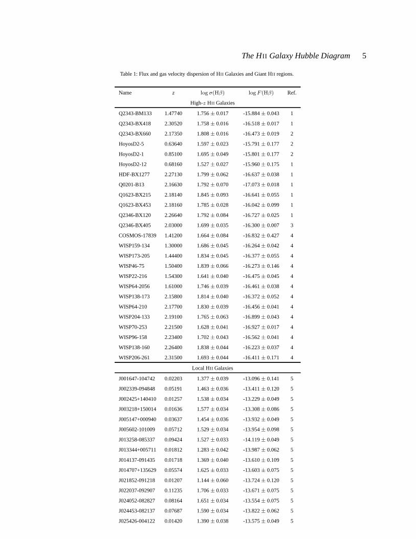
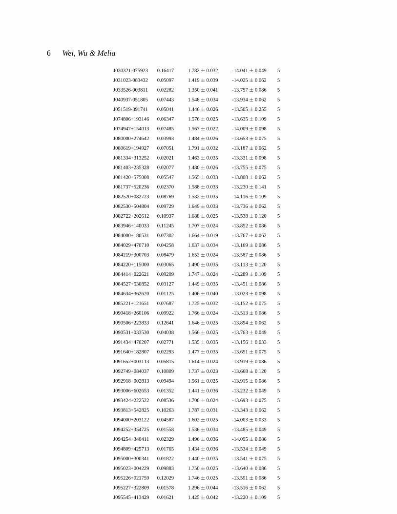
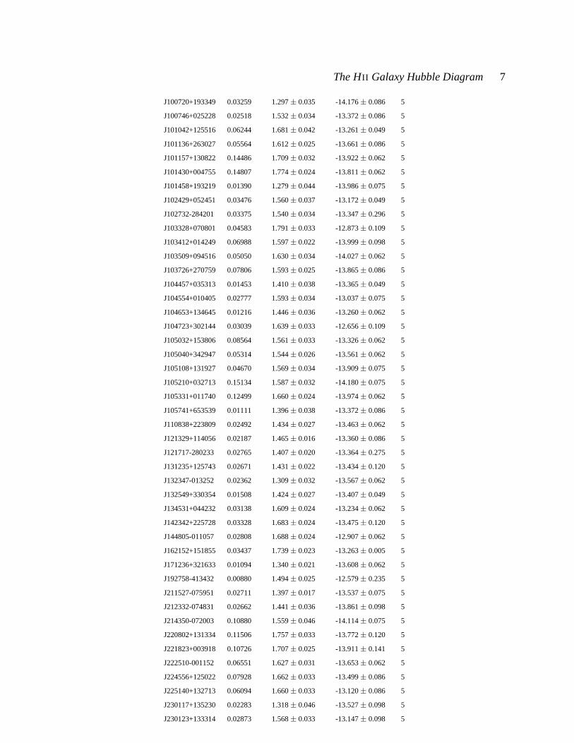
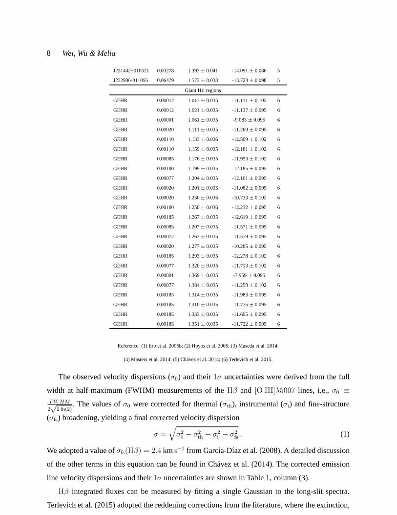
Table 1: Flux and gas velocity dispersion of HII Galaxies and Giant HII regions.

Name z log σ(Hβ) logF (Hβ) Ref.

High-z HII Galaxies

Q2343-BM133 1.47740 1.756± 0.017 -15.884± 0.043 1

Q2343-BX418 2.30520 1.758± 0.016 -16.518± 0.017 1

Q2343-BX660 2.17350 1.808± 0.016 -16.473± 0.019 2

HoyosD2-5 0.63640 1.597± 0.023 -15.791± 0.177 2

HoyosD2-1 0.85100 1.695± 0.049 -15.801± 0.177 2

HoyosD2-12 0.68160 1.527± 0.027 -15.960± 0.175 1

HDF-BX1277 2.27130 1.799± 0.062 -16.637± 0.038 1

Q0201-B13 2.16630 1.792± 0.070 -17.073± 0.018 1

Q1623-BX215 2.18140 1.845± 0.093 -16.641± 0.055 1

Q1623-BX453 2.18160 1.785± 0.028 -16.042± 0.099 1

Q2346-BX120 2.26640 1.792± 0.084 -16.727± 0.025 1

Q2346-BX405 2.03000 1.699± 0.035 -16.300± 0.007 3

COSMOS-17839 1.41200 1.664± 0.084 -16.832± 0.427 4

WISP159-134 1.30000 1.686± 0.045 -16.264± 0.042 4

WISP173-205 1.44400 1.834± 0.045 -16.377± 0.055 4

WISP46-75 1.50400 1.839± 0.066 -16.273± 0.146 4

WISP22-216 1.54300 1.641± 0.040 -16.475± 0.045 4

WISP64-2056 1.61000 1.746± 0.039 -16.461± 0.038 4

WISP138-173 2.15800 1.814± 0.040 -16.372± 0.052 4

WISP64-210 2.17700 1.830± 0.039 -16.456± 0.041 4

WISP204-133 2.19100 1.765± 0.063 -16.899± 0.043 4

WISP70-253 2.21500 1.628± 0.041 -16.927± 0.017 4

WISP96-158 2.23400 1.702± 0.043 -16.562± 0.041 4

WISP138-160 2.26400 1.838± 0.044 -16.223± 0.037 4

WISP206-261 2.31500 1.693± 0.044 -16.411± 0.171 4

Local HII Galaxies

J001647-104742 0.02203 1.377± 0.039 -13.096± 0.141 5

J002339-094848 0.05191 1.463± 0.036 -13.411± 0.120 5

J002425+140410 0.01257 1.538± 0.034 -13.229± 0.049 5

J003218+150014 0.01636 1.577± 0.034 -13.308± 0.086 5

J005147+000940 0.03637 1.454± 0.036 -13.932± 0.049 5

J005602-101009 0.05712 1.529± 0.034 -13.954± 0.098 5

J013258-085337 0.09424 1.527± 0.033 -14.119± 0.049 5

J013344+005711 0.01812 1.283± 0.042 -13.987± 0.062 5

J014137-091435 0.01718 1.369± 0.040 -13.610± 0.109 5

J014707+135629 0.05574 1.625± 0.033 -13.603± 0.075 5

J021852-091218 0.01207 1.144± 0.060 -13.724± 0.120 5

J022037-092907 0.11235 1.706± 0.033 -13.671± 0.075 5

J024052-082827 0.08164 1.651± 0.034 -13.554± 0.075 5

J024453-082137 0.07687 1.590± 0.034 -13.822± 0.062 5

J025426-004122 0.01420 1.390± 0.038 -13.575± 0.049 5

c© 0000 RAS, MNRAS000, 000–000

6 Wei, Wu & Melia

J030321-075923 0.16417 1.782± 0.032 -14.041± 0.049 5

J031023-083432 0.05097 1.419± 0.039 -14.025± 0.062 5

J033526-003811 0.02282 1.350± 0.041 -13.757± 0.086 5

J040937-051805 0.07443 1.548± 0.034 -13.934± 0.062 5

J051519-391741 0.05041 1.446± 0.026 -13.505± 0.255 5

J074806+193146 0.06347 1.576± 0.025 -13.635± 0.109 5

J074947+154013 0.07485 1.567± 0.022 -14.009± 0.098 5

J080000+274642 0.03993 1.484± 0.026 -13.653± 0.075 5

J080619+194927 0.07051 1.791± 0.032 -13.187± 0.062 5

J081334+313252 0.02021 1.463± 0.035 -13.331± 0.098 5

J081403+235328 0.02077 1.480± 0.026 -13.755± 0.075 5

J081420+575008 0.05547 1.565± 0.033 -13.808± 0.062 5

J081737+520236 0.02370 1.588± 0.033 -13.230± 0.141 5

J082520+082723 0.08769 1.532± 0.035 -14.116± 0.109 5

J082530+504804 0.09729 1.649± 0.033 -13.736± 0.062 5

J082722+202612 0.10937 1.688± 0.025 -13.538± 0.120 5

J083946+140033 0.11245 1.707± 0.024 -13.852± 0.086 5

J084000+180531 0.07302 1.664± 0.019 -13.767± 0.062 5

J084029+470710 0.04258 1.637± 0.034 -13.169± 0.086 5

J084219+300703 0.08479 1.652± 0.024 -13.587± 0.086 5

J084220+115000 0.03065 1.490± 0.035 -13.113± 0.120 5

J084414+022621 0.09209 1.747± 0.024 -13.289± 0.109 5

J084527+530852 0.03127 1.449± 0.035 -13.451± 0.086 5

J084634+362620 0.01125 1.406± 0.040 -13.023± 0.098 5

J085221+121651 0.07687 1.725± 0.032 -13.152± 0.075 5

J090418+260106 0.09922 1.766± 0.024 -13.513± 0.086 5

J090506+223833 0.12641 1.646± 0.025 -13.894± 0.062 5

J090531+033530 0.04038 1.566± 0.025 -13.763± 0.049 5

J091434+470207 0.02771 1.535± 0.035 -13.156± 0.033 5

J091640+182807 0.02293 1.477± 0.035 -13.651± 0.075 5

J091652+003113 0.05815 1.614± 0.024 -13.919± 0.086 5

J092749+084037 0.10809 1.737± 0.023 -13.668± 0.120 5

J092918+002813 0.09494 1.561± 0.025 -13.915± 0.086 5

J093006+602653 0.01352 1.441± 0.036 -13.232± 0.049 5

J093424+222522 0.08536 1.700± 0.024 -13.693± 0.075 5

J093813+542825 0.10263 1.787± 0.031 -13.343± 0.062 5

J094000+203122 0.04587 1.602± 0.025 -14.003± 0.033 5

J094252+354725 0.01558 1.536± 0.034 -13.485± 0.049 5

J094254+340411 0.02329 1.496± 0.036 -14.095± 0.086 5

J094809+425713 0.01765 1.434± 0.036 -13.534± 0.049 5

J095000+300341 0.01822 1.440± 0.035 -13.541± 0.075 5

J095023+004229 0.09883 1.750± 0.025 -13.640± 0.086 5

J095226+021759 0.12029 1.746± 0.025 -13.591± 0.086 5

J095227+322809 0.01578 1.296± 0.044 -13.516± 0.062 5

J095545+413429 0.01621 1.425± 0.042 -13.220± 0.109 5

c© 0000 RAS, MNRAS000, 000–000

The HII Galaxy Hubble Diagram 7

J100720+193349 0.03259 1.297± 0.035 -14.176± 0.086 5

J100746+025228 0.02518 1.532± 0.034 -13.372± 0.086 5

J101042+125516 0.06244 1.681± 0.042 -13.261± 0.049 5

J101136+263027 0.05564 1.612± 0.025 -13.661± 0.086 5

J101157+130822 0.14486 1.709± 0.032 -13.922± 0.062 5

J101430+004755 0.14807 1.774± 0.024 -13.811± 0.062 5

J101458+193219 0.01390 1.279± 0.044 -13.986± 0.075 5

J102429+052451 0.03476 1.560± 0.037 -13.172± 0.049 5

J102732-284201 0.03375 1.540± 0.034 -13.347± 0.296 5

J103328+070801 0.04583 1.791± 0.033 -12.873± 0.109 5

J103412+014249 0.06988 1.597± 0.022 -13.999± 0.098 5

J103509+094516 0.05050 1.630± 0.034 -14.027± 0.062 5

J103726+270759 0.07806 1.593± 0.025 -13.865± 0.086 5

J104457+035313 0.01453 1.410± 0.038 -13.365± 0.049 5

J104554+010405 0.02777 1.593± 0.034 -13.037± 0.075 5

J104653+134645 0.01216 1.446± 0.036 -13.260± 0.062 5

J104723+302144 0.03039 1.639± 0.033 -12.656± 0.109 5

J105032+153806 0.08564 1.561± 0.033 -13.326± 0.062 5

J105040+342947 0.05314 1.544± 0.026 -13.561± 0.062 5

J105108+131927 0.04670 1.569± 0.034 -13.909± 0.075 5

J105210+032713 0.15134 1.587± 0.032 -14.180± 0.075 5

J105331+011740 0.12499 1.660± 0.024 -13.974± 0.062 5

J105741+653539 0.01111 1.396± 0.038 -13.372± 0.086 5

J110838+223809 0.02492 1.434± 0.027 -13.463± 0.062 5

J121329+114056 0.02187 1.465± 0.016 -13.360± 0.086 5

J121717-280233 0.02765 1.407± 0.020 -13.364± 0.275 5

J131235+125743 0.02671 1.431± 0.022 -13.434± 0.120 5

J132347-013252 0.02362 1.309± 0.032 -13.567± 0.062 5

J132549+330354 0.01508 1.424± 0.027 -13.407± 0.049 5

J134531+044232 0.03138 1.609± 0.024 -13.234± 0.062 5

J142342+225728 0.03328 1.683± 0.024 -13.475± 0.120 5

J144805-011057 0.02808 1.688± 0.024 -12.907± 0.062 5

J162152+151855 0.03437 1.739± 0.023 -13.263± 0.005 5

J171236+321633 0.01094 1.340± 0.021 -13.608± 0.062 5

J192758-413432 0.00880 1.494± 0.025 -12.579± 0.235 5

J211527-075951 0.02711 1.397± 0.017 -13.537± 0.075 5

J212332-074831 0.02662 1.441± 0.036 -13.861± 0.098 5

J214350-072003 0.10880 1.559± 0.046 -14.114± 0.075 5

J220802+131334 0.11506 1.757± 0.033 -13.772± 0.120 5

J221823+003918 0.10726 1.707± 0.025 -13.911± 0.141 5

J222510-001152 0.06551 1.627± 0.031 -13.653± 0.062 5

J224556+125022 0.07928 1.662± 0.033 -13.499± 0.086 5

J225140+132713 0.06094 1.660± 0.033 -13.120± 0.086 5

J230117+135230 0.02283 1.318± 0.046 -13.527± 0.098 5

J230123+133314 0.02873 1.568± 0.033 -13.147± 0.098 5

c© 0000 RAS, MNRAS000, 000–000

8 Wei, Wu & Melia

J231442+010621 0.03278 1.393± 0.041 -14.091± 0.086 5

J232936-011056 0.06479 1.573± 0.033 -13.723± 0.098 5

Giant HII regions

GEHR 0.00012 1.013± 0.035 -11.131± 0.102 6

GEHR 0.00012 1.021± 0.035 -11.137± 0.095 6

GEHR 0.00001 1.061± 0.035 -9.083± 0.095 6

GEHR 0.00020 1.111± 0.035 -11.269± 0.095 6

GEHR 0.00110 1.133± 0.036 -12.509± 0.102 6

GEHR 0.00110 1.159± 0.035 -12.181± 0.102 6

GEHR 0.00085 1.176± 0.035 -11.953± 0.102 6

GEHR 0.00100 1.199± 0.035 -12.185± 0.095 6

GEHR 0.00077 1.204± 0.035 -12.101± 0.095 6

GEHR 0.00020 1.201± 0.035 -11.082± 0.095 6

GEHR 0.00020 1.250± 0.036 -10.733± 0.102 6

GEHR 0.00100 1.250± 0.036 -12.232± 0.095 6

GEHR 0.00185 1.267± 0.035 -12.619± 0.095 6

GEHR 0.00085 1.207± 0.035 -11.571± 0.095 6

GEHR 0.00077 1.267± 0.035 -11.579± 0.095 6

GEHR 0.00020 1.277± 0.035 -10.285± 0.095 6

GEHR 0.00185 1.293± 0.035 -12.278± 0.102 6

GEHR 0.00077 1.320± 0.035 -11.713± 0.102 6

GEHR 0.00001 1.369± 0.035 -7.959± 0.095 6

GEHR 0.00077 1.384± 0.035 -11.258± 0.102 6

GEHR 0.00185 1.314± 0.035 -11.983± 0.095 6

GEHR 0.00185 1.310± 0.035 -11.775± 0.095 6

GEHR 0.00185 1.333± 0.035 -11.695± 0.095 6

GEHR 0.00185 1.351± 0.035 -11.722± 0.095 6

Reference: (1) Erb et al. 2006b; (2) Hoyos et al. 2005; (3) Maseda et al. 2014;

(4) Masters et al. 2014; (5) Chavez et al. 2014; (6) Terlevich et al. 2015.

The observed velocity dispersions (σ0) and their1σ uncertainties were derived from the full

width at half-maximum (FWHM) measurements of theHβ and [O III]λ5007 lines, i.e.,σ0 ≡FWHM

2√

2 ln(2). The values ofσ0 were corrected for thermal (σth), instrumental (σi) and fine-structure

(σfs) broadening, yielding a final corrected velocity dispersion

σ =√

σ20 − σ2

th − σ2i − σ2

fs . (1)

We adopted a value ofσfs(Hβ) = 2.4 km s−1 from Garcıa-Dıaz et al. (2008). A detailed discussion

of the other terms in this equation can be found in Chavez et al. (2014). The corrected emission

line velocity dispersions and their1σ uncertainties are shown in Table 1, column (3).

Hβ integrated fluxes can be measured by fitting a single Gaussianto the long-slit spectra.

Terlevich et al. (2015) adopted the reddening corrections from the literature, where the extinction,

c© 0000 RAS, MNRAS000, 000–000

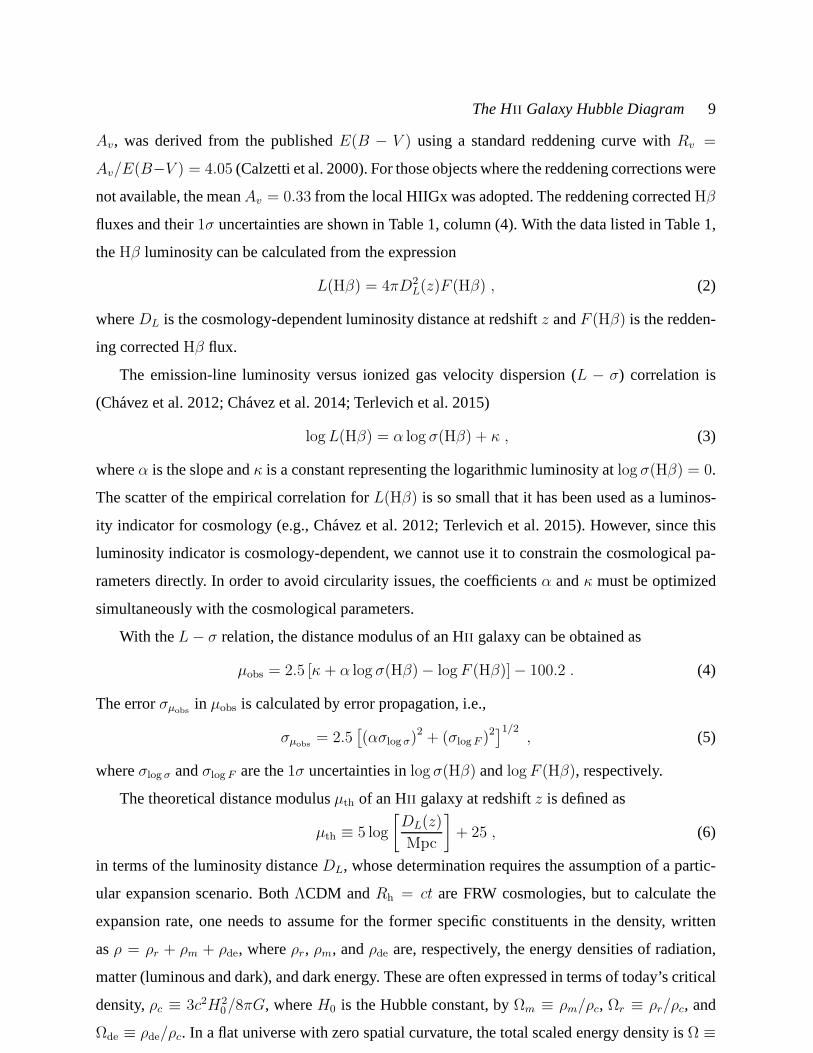
The HII Galaxy Hubble Diagram 9

Av, was derived from the publishedE(B − V ) using a standard reddening curve withRv =

Av/E(B−V ) = 4.05 (Calzetti et al. 2000). For those objects where the reddening corrections were

not available, the meanAv = 0.33 from the local HIIGx was adopted. The reddening correctedHβ

fluxes and their1σ uncertainties are shown in Table 1, column (4). With the datalisted in Table 1,

theHβ luminosity can be calculated from the expression

L(Hβ) = 4πD2L(z)F (Hβ) , (2)

whereDL is the cosmology-dependent luminosity distance at redshift z andF (Hβ) is the redden-

ing correctedHβ flux.

The emission-line luminosity versus ionized gas velocity dispersion (L − σ) correlation is

(Chavez et al. 2012; Chavez et al. 2014; Terlevich et al. 2015)

logL(Hβ) = α log σ(Hβ) + κ , (3)

whereα is the slope andκ is a constant representing the logarithmic luminosity atlog σ(Hβ) = 0.

The scatter of the empirical correlation forL(Hβ) is so small that it has been used as a luminos-

ity indicator for cosmology (e.g., Chavez et al. 2012; Terlevich et al. 2015). However, since this

luminosity indicator is cosmology-dependent, we cannot use it to constrain the cosmological pa-

rameters directly. In order to avoid circularity issues, the coefficientsα andκ must be optimized

simultaneously with the cosmological parameters.

With theL− σ relation, the distance modulus of an HII galaxy can be obtained as

µobs = 2.5 [κ + α log σ(Hβ)− logF (Hβ)]− 100.2 . (4)

The errorσµobsin µobs is calculated by error propagation, i.e.,

σµobs= 2.5

[

(ασlog σ)2 + (σlogF )

2]1/2 , (5)

whereσlog σ andσlog F are the1σ uncertainties inlog σ(Hβ) andlogF (Hβ), respectively.

The theoretical distance modulusµth of an HII galaxy at redshiftz is defined as

µth ≡ 5 log

[

DL(z)

Mpc

]

+ 25 , (6)

in terms of the luminosity distanceDL, whose determination requires the assumption of a partic-

ular expansion scenario. BothΛCDM andRh = ct are FRW cosmologies, but to calculate the

expansion rate, one needs to assume for the former specific constituents in the density, written

asρ = ρr + ρm + ρde, whereρr, ρm, andρde are, respectively, the energy densities of radiation,

matter (luminous and dark), and dark energy. These are oftenexpressed in terms of today’s critical

density,ρc ≡ 3c2H20/8πG, whereH0 is the Hubble constant, byΩm ≡ ρm/ρc, Ωr ≡ ρr/ρc, and

Ωde ≡ ρde/ρc. In a flat universe with zero spatial curvature, the total scaled energy density isΩ ≡c© 0000 RAS, MNRAS000, 000–000

10 Wei, Wu & Melia

Ωm + Ωr + Ωde = 1. In Rh = ct, on the other hand, whatever constituents are present inρ, the

principal constraint is the total equation-of-statep = −ρ/3.

In ΛCDM, the luminosity distance is given as

DΛCDML (z) =

c

H0

(1 + z)√

| Ωk |sinn

| Ωk |1/2∫ z

0

dz√

Ωm(1 + z)3 + Ωk(1 + z)2 + Ωde(1 + z)3(1+wde)

,

(7)

wherepde = wdeρde is the dark-energy equation of state, and we have assumed that the radiation

density is negligible in the local Universe. Also,Ωk = 1 − Ωm − Ωde represents the spatial cur-

vature of the Universe—appearing as a term proportional to the spatial curvature constantk in

the Friedmann equation. In addition, sinn issinh whenΩk > 0 andsin whenΩk < 0. For a flat

Universe (Ωk = 0), the right side becomes(1 + z)c/H0 times the indefinite integral.

In theRh = ct Universe (Melia 2003, 2007, 2013a, 2016a, 2016b; Melia & Abdelqader 2009;

Melia & Shevchuk 2012), the luminosity distance is given by the much simpler expression

DRh=ctL (z) =

c

H0

(1 + z) ln(1 + z) . (8)

To find the best-fit cosmological parameters and (simultaneously) the coefficientsα andκ,

we adopt the method of maximum likelihood estimation (MLE; see Wei et al. 2015b). The joint

likelihood function for all these parameters, based on a flatBayesian prior, is

L =∏

i

1√2π σµobs,i

× exp

[

− (µobs,i − µth(zi))2

2σ2µobs,i

]

. (9)

Because the first factorσµobsin the product of Equation (9) is not a constant, dependent onthe

value ofα (see Equation 5), maximizing the likelihood functionL is not exactly equivalent to

minimizing theχ2 statistic, i.e.,χ2 =∑

i

(µobs,i−µth(zi))2

σ2µobs,i

.

In MLE, the chosen value ofH0 is not independent ofκ. That is, one can vary eitherH0 or κ,

but not both. Therefore, we adopt a definition

δ ≡ −2.5κ− 5 logH0 + 125.2 , (10)

whereδ is the “H0-free” logarithmic luminosity andH0 is in units of kms−1 Mpc−1. With this

definition, the likelihood function becomes

L =∏

i

1√2π σµobs,i

× exp

[

− ∆2i

2σ2µobs,i

]

, (11)

where∆i = 2.5 [α log σ(Hβ)i − logF (Hβ)i] − δ − 5 log [H0DL(zi)], with DL the luminosity

distance in Mpc. The Hubble constantH0 cancels out in Equation (11) when we multiplyDL by

H0, so the constraints on the cosmological parameters are independent of the Hubble constant. In

this paper,α andδ are statistical “nuisance” parameters.

c© 0000 RAS, MNRAS000, 000–000

The HII Galaxy Hubble Diagram 11

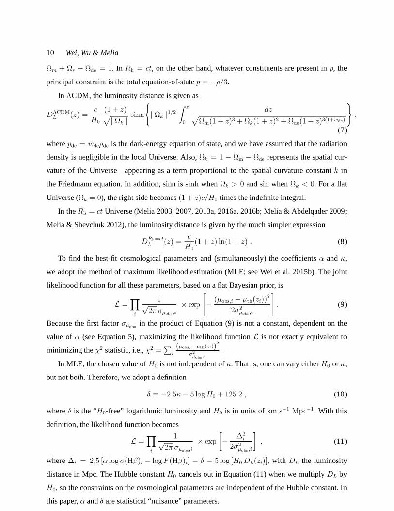
Figure 1. 1-D probability distributions and 2-D regions with the1-3σ contours corresponding to the parametersα, δ andΩm in the flatΛCDMmodel.

To constrain the nuisance parameters and cosmological parameters simultaneously, we use

the Markov Chain Monte Carlo (MCMC) technique. Our MCMC approach generates a chain

of sample points distributed in parameter space according to the posterior probability, using the

Metropolis-Hastings algorithm with uniform prior distributions. For each Markov chain, we gen-

erate105 samples based on the likelihood function. Then we adopt the publicly available package

“triangle.py” developed by Foreman-Mackey et al. (2013) toplot 1-D marginalized probability

distributions and 2-D contours.

3 OPTIMIZATION OF THE MODEL PARAMETERS

We use the HII galaxies as standardizable candles and apply the emission-line luminosity versus

ionized gas velocity dispersion (L− σ) relation (with 156 objects) to compare the standard model

with the Rh = ct Universe. In this section, we discuss how the fits have been optimized for

ΛCDM, wCDM andRh = ct. The outcome for each model is more fully described and discussed

in subsequent sections.

c© 0000 RAS, MNRAS000, 000–000

12 Wei, Wu & Melia

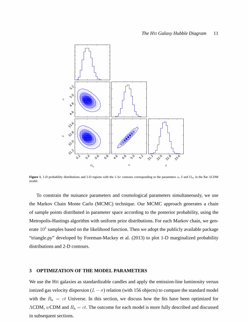
Figure 2. 1-D probability distributions and 2-D regions with the1-3σ contours corresponding to the parametersΩm, wde, α, andδ in the best-fitwCDM model.

3.1 ΛCDM

In the most basicΛCDM model, the dark-energy equation of state parameter,wde, is exactly−1.

The Hubble constantH0 cancels out in Equation (11) when we multiplyDL byH0, so the essential

remaining parameter in flatΛCDM (with Ωk = 0) isΩm. The resulting constraints onα, δ, andΩm

are shown in Figure 1. These contours show that at the1σ level, the optimized parameter values

areα = 4.89+0.09−0.09 (1σ), δ = 32.49+0.35

−0.35 (1σ), andΩm = 0.40+0.09−0.09 (1σ). The maximum value of

the joint likelihood function for the optimized flatΛCDM model is given by−2 lnL = 563.77,

which we shall need when comparing models using the information criteria.

3.2 wCDM

To allow for the greatest flexibility in this fit, we relax the assumption that dark energy is a cos-

mological constant withwde = −1, and allowwde to be free along withΩm. The optimized pa-

rameters corresponding to the best-fitwCDM model for these 156 data are displayed in Figure 2,

which shows the 1-D probability distribution for each parameter (Ωm, wde, α, δ), and 2-D plots

c© 0000 RAS, MNRAS000, 000–000

The HII Galaxy Hubble Diagram 13

Figure 3. 1-3σ constraints onα andδ for theRh = ct Universe.

of the 1-3σ confidence regions for two-parameter combinations. The best-fit values forwCDM

areΩm = 0.22+0.16−0.14 (1σ), wde = −0.51+0.15

−0.25 (1σ), α = 4.87+0.10−0.09 (1σ), andδ = 32.40+0.36

−0.36 (1σ).

The maximum value of the joint likelihood function for the optimizedwCDM model is given by

−2 lnL = 561.12.

3.3 The Rh = ct Universe

TheRh = ct Universe has only one free parameter,H0, but since the Hubble constant cancels out

in the productH0DL, there are actually no free (model) parameters left to fit theHII galaxy data.

The results of fitting theL − σ relation with this cosmology are shown in Figure 3. We see here

that the best fit corresponds toα = 4.86+0.08−0.07 (1σ) andδ = 32.38+0.29

−0.29 (1σ). The maximum value

of the joint likelihood function for the optimizedRh = ct fit corresponds to−2 lnL = 559.98.

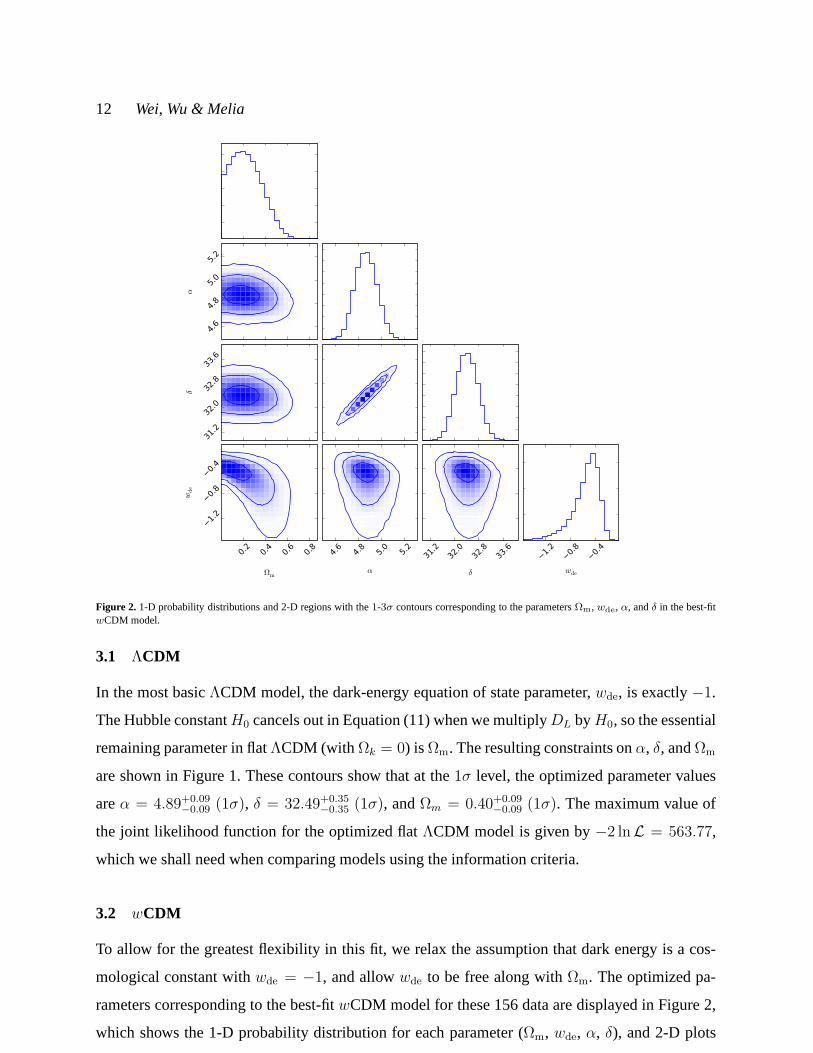
4 THE HII GALAXY HUBBLE DIAGRAM

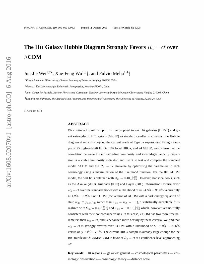
To facilitate a direct comparison betweenΛCDM andRh = ct, we show in Figure 4 the Hubble

diagrams for the combined 25 high-z HII galaxies and the 131 local sample (107 HII galaxies and

24 Giant Extragalactic HII Regions). In this figure, the observed distance moduli of 156objects

are plotted as solid points, together with the best-fit theoretical curves (from left to right) for the

optimized flatΛCDM model (withΩm = 0.40, α = 4.89, andδ = 32.49) and for theRh = ct

Universe (withα = 4.86 andδ = 32.38). For completeness, the lower panels in Figure 4 also

show the Hubble diagram residuals relative to the best-fit cosmological models.

An inspection of the Hubble diagrams in Figures 4 reveals that both the optimizedΛCDM

c© 0000 RAS, MNRAS000, 000–000

14 Wei, Wu & Melia

20

25

30

35

40

45

50

10-5 10-4 10-3 10-2 10-1 100

-2

-1

0

1

2

CDM

GEHR local HIIGx high-z HIIGx

z

Res

idua

ls

20

25

30

35

40

45

50

10-5 10-4 10-3 10-2 10-1 100

-2

-1

0

1

2

Rh=ct

GEHR local HIIGx high-z HIIGx

Res

idua

ls

z

Figure 4. Left: Hubble diagram and Hubble diagram residuals for the 156 combined sources (including 25 high-z HII galaxies, 107 local HII galax-ies, and 24 Giant Extragalactic HII Regions) optimized for the flatΛCDM model. Right: Same as the left panel, but now for theRh = ct Universe.

model and theRh = ct Universe fit their respective data sets very well. However, because these

models formulate their observables (such as the luminositydistances in Equations 7 and 8) dif-

ferently, and because they do not have the same number of freeparameters, a comparison of the

likelihoods for either being closer to the ‘true’ model mustbe based on model selection tools.

Several model selection tools commonly used to differentiate between cosmological models

(see, e.g., Melia & Maier 2013, and references cited therein) include the Akaike Information Cri-

terion,AIC = −2 lnL + 2n, wheren is the number of free parameters (Akaike 1973; Liddle

2007; see also Burnham & Anderson 2002, 2004), the Kullback Information Criterion,KIC =

−2 lnL+3n (Cavanaugh 2004), and the Bayes Information Criterion,BIC = −2 lnL+(lnN)n,

whereN is the number of data points (Schwarz 1978). In the case of AIC, with AICα charac-

terizing modelMα, the unnormalized confidence that this model is true is the Akaike weight

exp(−AICα/2). ModelMα has likelihood

P (Mα) =exp(−AICα/2)

exp(−AIC1/2) + exp(−AIC2/2)(12)

of being the correct choice in this one-on-one comparison. Thus, the difference∆AIC ≡ AIC2 −AIC1 determines the extent to whichM1 is favored overM2. For Kullback and Bayes, the like-

lihoods are defined analogously. In using the model selection tools, the outcome∆ ≡ AIC1−AIC2 (and analogously for KIC and BIC) is judged ‘positive’ in therange∆ = 2− 6, ‘strong’ for

∆ = 6− 10, and ‘very strong’ for∆ > 10.

With the optimized fits of theL−σ relation (using 156 objects), the magnitude of the difference

∆AIC = AIC2 − AIC1 = 5.79, indicates thatRh = ct (i.e.M1) is to be preferred over the flat

c© 0000 RAS, MNRAS000, 000–000

The HII Galaxy Hubble Diagram 15

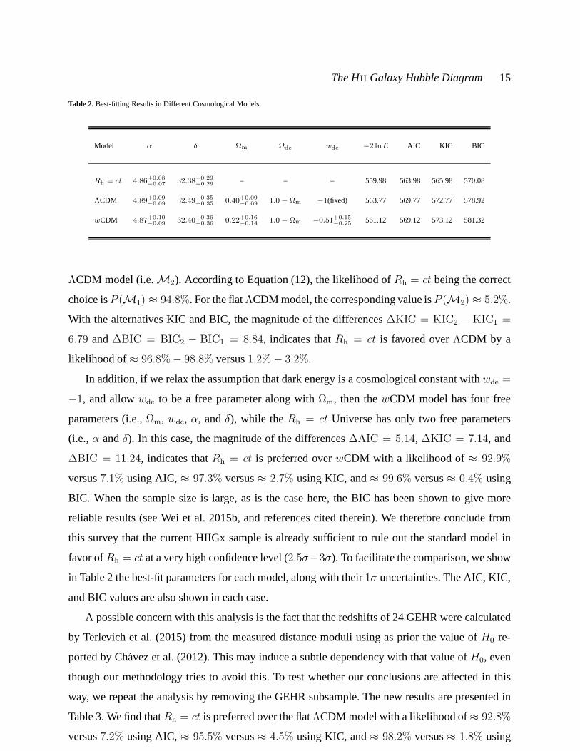
Table 2. Best-fitting Results in Different Cosmological Models

Model α δ Ωm Ωde wde −2 lnL AIC KIC BIC

Rh = ct 4.86+0.08−0.07

32.38+0.29−0.29

– – – 559.98 563.98 565.98 570.08

ΛCDM 4.89+0.09−0.09

32.49+0.35−0.35

0.40+0.09−0.09

1.0− Ωm −1(fixed) 563.77 569.77 572.77 578.92

wCDM 4.87+0.10−0.09

32.40+0.36−0.36

0.22+0.16−0.14

1.0− Ωm −0.51+0.15−0.25

561.12 569.12 573.12 581.32

ΛCDM model (i.e.M2). According to Equation (12), the likelihood ofRh = ct being the correct

choice isP (M1) ≈ 94.8%. For the flatΛCDM model, the corresponding value isP (M2) ≈ 5.2%.

With the alternatives KIC and BIC, the magnitude of the differences∆KIC = KIC2 − KIC1 =

6.79 and∆BIC = BIC2 − BIC1 = 8.84, indicates thatRh = ct is favored overΛCDM by a

likelihood of≈ 96.8%− 98.8% versus1.2%− 3.2%.

In addition, if we relax the assumption that dark energy is a cosmological constant withwde =

−1, and allowwde to be a free parameter along withΩm, then thewCDM model has four free

parameters (i.e.,Ωm, wde, α, andδ), while theRh = ct Universe has only two free parameters

(i.e.,α andδ). In this case, the magnitude of the differences∆AIC = 5.14, ∆KIC = 7.14, and

∆BIC = 11.24, indicates thatRh = ct is preferred overwCDM with a likelihood of≈ 92.9%

versus7.1% using AIC,≈ 97.3% versus≈ 2.7% using KIC, and≈ 99.6% versus≈ 0.4% using

BIC. When the sample size is large, as is the case here, the BIChas been shown to give more

reliable results (see Wei et al. 2015b, and references citedtherein). We therefore conclude from

this survey that the current HIIGx sample is already sufficient to rule out the standard model in

favor ofRh = ct at a very high confidence level (2.5σ−3σ). To facilitate the comparison, we show

in Table 2 the best-fit parameters for each model, along with their1σ uncertainties. The AIC, KIC,

and BIC values are also shown in each case.

A possible concern with this analysis is the fact that the redshifts of 24 GEHR were calculated

by Terlevich et al. (2015) from the measured distance moduliusing as prior the value ofH0 re-

ported by Chavez et al. (2012). This may induce a subtle dependency with that value ofH0, even

though our methodology tries to avoid this. To test whether our conclusions are affected in this

way, we repeat the analysis by removing the GEHR subsample. The new results are presented in

Table 3. We find thatRh = ct is preferred over the flatΛCDM model with a likelihood of≈ 92.8%

versus7.2% using AIC,≈ 95.5% versus≈ 4.5% using KIC, and≈ 98.2% versus≈ 1.8% using

c© 0000 RAS, MNRAS000, 000–000

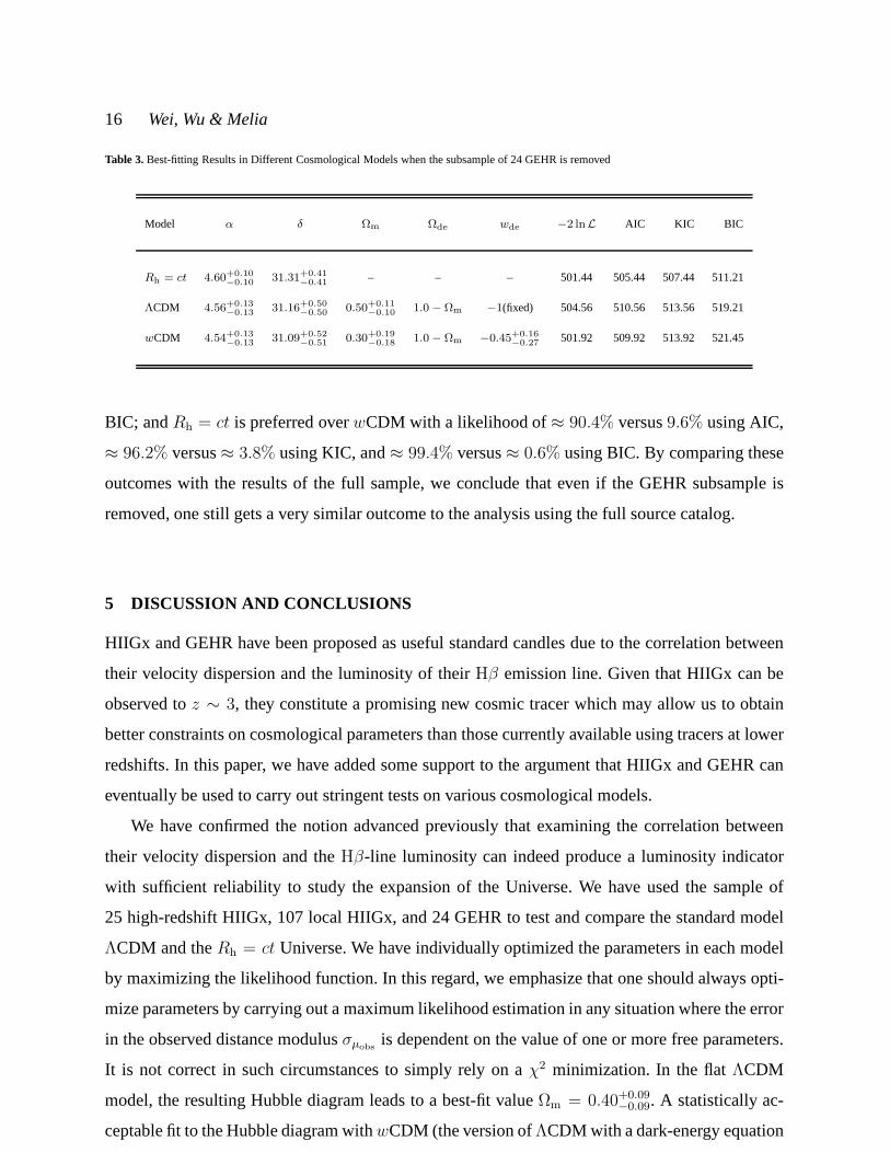
16 Wei, Wu & Melia

Table 3. Best-fitting Results in Different Cosmological Models whenthe subsample of 24 GEHR is removed

Model α δ Ωm Ωde wde −2 lnL AIC KIC BIC

Rh = ct 4.60+0.10−0.10

31.31+0.41−0.41

– – – 501.44 505.44 507.44 511.21

ΛCDM 4.56+0.13−0.13

31.16+0.50−0.50

0.50+0.11−0.10

1.0− Ωm −1(fixed) 504.56 510.56 513.56 519.21

wCDM 4.54+0.13−0.13

31.09+0.52−0.51

0.30+0.19−0.18

1.0− Ωm −0.45+0.16−0.27

501.92 509.92 513.92 521.45

BIC; andRh = ct is preferred overwCDM with a likelihood of≈ 90.4% versus9.6% using AIC,

≈ 96.2% versus≈ 3.8% using KIC, and≈ 99.4% versus≈ 0.6% using BIC. By comparing these

outcomes with the results of the full sample, we conclude that even if the GEHR subsample is

removed, one still gets a very similar outcome to the analysis using the full source catalog.

5 DISCUSSION AND CONCLUSIONS

HIIGx and GEHR have been proposed as useful standard candlesdue to the correlation between

their velocity dispersion and the luminosity of theirHβ emission line. Given that HIIGx can be

observed toz ∼ 3, they constitute a promising new cosmic tracer which may allow us to obtain

better constraints on cosmological parameters than those currently available using tracers at lower

redshifts. In this paper, we have added some support to the argument that HIIGx and GEHR can

eventually be used to carry out stringent tests on various cosmological models.

We have confirmed the notion advanced previously that examining the correlation between

their velocity dispersion and theHβ-line luminosity can indeed produce a luminosity indicator

with sufficient reliability to study the expansion of the Universe. We have used the sample of

25 high-redshift HIIGx, 107 local HIIGx, and 24 GEHR to test and compare the standard model

ΛCDM and theRh = ct Universe. We have individually optimized the parameters ineach model

by maximizing the likelihood function. In this regard, we emphasize that one should always opti-

mize parameters by carrying out a maximum likelihood estimation in any situation where the error

in the observed distance modulusσµobsis dependent on the value of one or more free parameters.

It is not correct in such circumstances to simply rely on aχ2 minimization. In the flatΛCDM

model, the resulting Hubble diagram leads to a best-fit valueΩm = 0.40+0.09−0.09. A statistically ac-

ceptable fit to the Hubble diagram withwCDM (the version ofΛCDM with a dark-energy equation

c© 0000 RAS, MNRAS000, 000–000

The HII Galaxy Hubble Diagram 17

of statewde ≡ pde/ρde rather thanwde = wΛ = −1) is possible only withΩm = 0.22+0.16−0.14 and

wde = −0.51+0.15−0.25. These values, however, are not fully consistent with the concordance model.

More importantly, we have found that, when the parameter optimization is handled via maxi-

mum likelihood optimization, the Akaike, Kullback and Bayes Information Criteria tend to favor

theRh = ct Universe. Since the flatΛCDM model (withΩm, α, andδ) has one more free pa-

rameter thanRh = ct (i.e.,α andδ), the latter is preferred over the former with a likelihood of

≈ 94.8% versus≈ 5.2% using AIC,≈ 96.8% versus≈ 3.2% using KIC, and≈ 98.8% versus

≈ 1.2% using BIC. If we relax the assumption that dark energy is a cosmological constant with

wde = −1, and allowwde to be a free parameter along withΩm, then thewCDM model has four

free parameters (i.e.,Ωm, wde, α, andδ). We find thatRh = ct is preferred overwCDM with a

likelihood of≈ 92.9% versus7.1% using AIC,≈ 97.3% versus≈ 2.7% using KIC, and≈ 99.6%

versus≈ 0.4% using BIC.

In other words, the current HIIGx sample is sufficient to ruleout the standard model in favor

of Rh = ct at a very high confidence level. The consequences of this important result are being

explored elsewhere, including the growing possibility that inflation may have been unnecessary to

resolve any perceived ‘horizon problem’ and therefore may have simply never happened (Melia

2013a).

We close this discussion by pointing out three important caveats to our conclusions. First,

since the cosmological parameters are more sensitive to thehigh-z observational data than the

low-z ones, most of the weight of the constraints obtained in this work (e.g., for the parameter

of the equation of state of dark energy) is from the high-z sample of only 25 HIIGx. Secondly,

the systematic uncertainties of theL(Hβ) − σ correlation need to be better understood, which

may affect HII galaxies as cosmological probes. The associated systematic uncertainties include

the size of the burst, the age of the burst, the oxygen abundance of HII galaxies, and the internal

extinction correction (Chavez et al. 2016).

Some progress has already been made with attempts at mitigating these uncertainties (Melnick

et al. 1988; Chavez et al. 2014), though efforts such as these also highlight the need to probe all

possible sources of systematic errors more deeply. For example, an important consideration is the

exclusion of rotationally supported systems, which clearly would skew theL(Hβ) − σ relation.

Melnick et al. (1988) and Chavez et al. (2014, 2016) have proposed using an upper limit to the

velocity dispersion oflog σ(Hβ) ∼ 1.8 km s−1 to minimize this possibility, though at a significant

cost—of greatly reducing the catalog of suitable sources. Nonetheless, even with this limit, there is

c© 0000 RAS, MNRAS000, 000–000

18 Wei, Wu & Melia

no guarantee that such a systematic effect is completely removed. As a second example, since the

L(Hβ)− σ relation is essentially a correlation between the ionizingflux produced by the massive

stars, and the velocity field in the potential well due to stars and gas, any systematic variation of

the initial mass function will affect the mass-luminosity ratio and therefore the slope and/or zero

point of the relation (Chavez et al. 2014).

A third important caveat is that our constraints are somewhat weaker than the results of some

other cosmological probes, and they have uncertainties because of the small HIIGx sample effect.

To increase the significance of the constraints, one needs a larger sample. Fortunately, with the help

of current facilities, such as the K-band Multi Object Spectrograph at the Very Large Telescope,

a larger sample of high-z HIIGx with high quality data will be observed in the near future, which

will provide much better and competitive constraints on thecosmological parameters (Terlevich et

al. 2015).

ACKNOWLEDGMENTS

We thank the anonymous referee for insightful comments thathave helped us improve the pre-

sentation of the paper. This work is partially supported by the National Basic Research Program

(“973” Program) of China (Grants 2014CB845800 and 2013CB834900), the National Natural Sci-

ence Foundation of China (grants Nos. 11322328 and 11373068), the Youth Innovation Promotion

Association (2011231), the Strategic Priority Research Program “The Emergence of Cosmolog-

ical Structures” (Grant No. XDB09000000) of the Chinese Academy of Sciences, the Natural

Science Foundation of Jiangsu Province (Grant No. BK20161096), and the Guangxi Key Labo-

ratory for Relativistic Astrophysics. F.M. is grateful to Amherst College for its support through a

John Woodruff Simpson Lectureship, and to Purple Mountain Observatory in Nanjing, China, for

its hospitality while part of this work was being carried out. This work was partially supported

by grant 2012T1J0011 from The Chinese Academy of Sciences Visiting Professorships for Se-

nior International Scientists, and grant GDJ20120491013 from the Chinese State Administration

of Foreign Experts Affairs.

REFERENCES

Abazajian K. N., et al., 2009, ApJS, 182, 543-558

Alcaniz J. S., Lima J. A. S., 1999, ApJ, 521, L87

c© 0000 RAS, MNRAS000, 000–000

The HII Galaxy Hubble Diagram 19

Akaike, H. 1973, in Second International Symposium on Information Theory, eds. B. N. Petrov

and F. Csaki (Budapest: Akademiai Kiado), 267

Burnham, K. P. & Anderson, D. R. 2002, Model Selection and Multimodel Inference, 2nd edn.

(New York: Springer-Verlag)

Burnham, K. P. & Anderson, D. R. 2004, Sociol. Methods Res., 33, 261

Bergeron J., 1977, ApJ, 211, 62

Bordalo V., Telles E., 2011, ApJ, 735, 52

Bosch G., Terlevich E., Terlevich R., 2002, MNRAS, 329, 481

Calzetti D., Armus L., Bohlin R. C., Kinney A. L., Koornneef J., Storchi-Bergmann T., 2000,

ApJ, 533, 682

Cavanaugh, J. E. 2004, Aust. N. Z. J. Stat., 46, 257

Chavez R., Terlevich R., Terlevich E., Bresolin F., Melnick J., Plionis M., Basilakos S., 2014,

MNRAS, 442, 3565

Chavez R., Terlevich E., Terlevich R., Plionis M., Bresolin F., Basilakos S., Melnick J., 2012,

MNRAS, 425, L56

Chavez R., Plionis M., Basilakos S., Terlevich R., Terlevich E., Melnick J., Bresolin F., Gonzalez-

Moran A. L., 2016, MNRAS in press, arXiv:1607.06458

Dai Z. G., Liang E. W., Xu D., 2004, ApJ, 612, L101

Erb D. K., Steidel C. C., Shapley A. E., Pettini M., Reddy N. A., Adelberger K. L., 2006a, ApJ,

647, 128

Erb D. K., Steidel C. C., Shapley A. E., Pettini M., Reddy N. A., Adelberger K. L., 2006b, ApJ,

646, 107

Foreman-Mackey D., Hogg D. W., Lang D., Goodman J., 2013, PASP, 125, 306

Fuentes-Masip O., Munoz-Tunon C., Castaneda H. O., Tenorio-Tagle G., 2000, AJ, 120, 752

Garcıa-Dıaz M. T., Henney W. J., Lopez J. A., Doi T., 2008,RMxAA, 44, 181

Ghirlanda G., Ghisellini G., Lazzati D., Firmani C., 2004, ApJ, 613, L13

Hoyos C., Koo D. C., Phillips A. C., Willmer C. N. A., Guhathakurta P., 2005, ApJ, 635, L21

Inserra C., Smartt S. J., 2014, ApJ, 796, 87

Jimenez R., Loeb A., 2002, ApJ, 573, 37

Kauffmann G., Haehnelt M., 2000, MNRAS, 311, 576

Kunth D.,Ostlin G., 2000, A&ARv, 10, 1

Liddle A. R., 2007, MNRAS, 377, L74

Lima J. A. S., Alcaniz J. S., 2000, MNRAS, 317, 893

c© 0000 RAS, MNRAS000, 000–000

20 Wei, Wu & Melia

Mania D., Ratra B., 2012, PhLB, 715, 9

Maseda M. V., et al., 2014, ApJ, 791, 17

Masters D., et al., 2014, ApJ, 785, 153

Melia F., 2003, “The Edge of Infinity: Supermassive Black Holes in the Universe” (New York:

Cambridge University Press), 158–171

Melia F., 2007, MNRAS, 382, 1917

Melia F., 2012, AJ, 144, 110

Melia F., 2013a, A&A, 553, A76

Melia F., 2013b, ApJ, 764, 72

Melia F., 2014, JCAP, 1, 027

Melia F., 2015, MNRAS, 446, 1191

Melia, F., 2016a, Frontiers of Physics, 11, 119801 (arXiv:1601.04991)

Melia, F., 2016b, Frontiers of Physics, in press (arXiv:1602.01435)

Melia F. and Abdelqader M., 2009, IJMPD, 18, 1889

Melia F. and Maier R. S., 2013, MNRAS, 432, 2669

Melia F. and McClintock T. M., 2015a, AJ, 150, 119

Melia F. and McClintock T. M., 2015b, Proc. R. Soc. A, 471, 20150449

Melia F. and Shevchuk A. S. H., 2012, MNRAS, 419, 2579

Melnick J., Moles M., Terlevich R., Garcia-Pelayo J.-M., 1987, MNRAS, 226, 849

Melnick J., Terlevich R., Moles M., 1988, MNRAS, 235, 297

Melnick J., Terlevich R., Terlevich E., 2000, MNRAS, 311, 629

Perlmutter S., et al., 1998, Natur, 391, 51

Plionis M., Terlevich R., Basilakos S., Bresolin F., Terlevich E., Melnick J., Chavez R., 2011,

MNRAS, 416, 2981

Riess A. G., et al., 1998, AJ, 116, 1009

Schmidt B. P., et al., 1998, ApJ, 507, 46

Schwarz, G. 1978, Ann. Statist., 6, 461

Searle L., Sargent W. L. W., 1972, ApJ, 173, 25

Siegel E. R., Guzman R., Gallego J. P., Orduna Lopez M., Rodrıguez Hidalgo P., 2005, MNRAS,

356, 1117

Simon J., Verde L., Jimenez R., 2005, PhRvD, 71, 123001

Telles E., 2003, ASPC, 297, 143

Terlevich R., Melnick J., 1981, MNRAS, 195, 839

c© 0000 RAS, MNRAS000, 000–000

The HII Galaxy Hubble Diagram 21

Terlevich R., Terlevich E., Melnick J., Chavez R., PlionisM., Bresolin F., Basilakos S., 2015,

MNRAS, 451, 3001

Wei J.-J., Wu X.-F., Melia F., 2013, ApJ, 772, 43

Wei J.-J., Wu X.-F., Melia F., 2015a, AJ, 149, 165

Wei J.-J., Wu X.-F., Melia F., Maier R. S., 2015b, AJ, 149, 102

Wei J.-J., Wu X.-F., Melia F., Wang F.-Y., Yu H., 2015c, AJ, 150, 35

Wyithe J. S. B., Loeb A., 2003, ApJ, 595, 614

c© 0000 RAS, MNRAS000, 000–000