arX

iv:a

stro

-ph/

0309

610

v2

29 S

ep 2

003

Mon. Not. R. Astron. Soc. 000, 000–000 (0000) Printed 30 September 2003 (MN LATEX style file v1.4)

Scientific optimization of a ground-based CMB

polarization experiment

M. Bowden,1⋆ A. N. Taylor,2† K. M. Ganga,3‡ P. A. R. Ade,1

J. J. Bock,5,6 G. Cahill,7 J. E. Carlstrom,8 S. E. Church,4 W. K. Gear,1

J. R. Hinderks,4 W. Hu,8 B. G. Keating,6 J. Kovac,6,8A .E. Lange,6 E. M. Leitch,8

B. Maffei,1 O. E. Mallie,1 S. J. Melhuish,1 J. A. Murphy,7 G. Pisano,1 L. Piccirillo,1

C. Pryke,8 B. A. Rusholme,4 C. O’Sullivan,7 K. Thompson4

1Department of Physics and Astronomy, University of Wales, Cardiff, PO Box 913, Cardiff, CF24 3YB2Institute for Astronomy, University of Edinburgh, Royal Observatory, Blackford Hill, Edinburgh, EH9 3HJ3Infrared Processing and Analysis Center, California Institute of Technology, Pasadena, CA 911254Department of Physics, Stanford University, Stanford, CA 943055Jet Propulsion Labratory, 4800 Oak Grove Dr., Pasadena, CA 911096Division of Physics, Math and Astronomy, California Institute of Technology, Pasadena, CA 911257Experimental Physics Department, National University of Ireland, Maynooth, Co. Kildare, Ireland8Department of Astronomy and Astrophysics, Department of Physics, Enrico Fermi Lab, University of Chicago,

5640 South Ellis Avenue, Chicago, IL 60637

30 September 2003

ABSTRACT

We investigate the science goals achievable with the upcoming generation of ground-based Cosmic Microwave Background polarization experiments and calculate the op-timal sky coverage for such an experiment including the effects of foregrounds. Wefind that with current technology an E-mode measurement will be sample-limited,while a B-mode measurement will be detector-noise-limited. We conclude that a 300deg2 survey is an optimal compromise for a two-year experiment to measure both Eand B-modes, and that ground-based polarization experiments can make an impor-tant contribution to B-mode surveys. Focusing on one particular experiment, QUaD, aproposed bolometric polarimeter operating from the South Pole, we find that a ground-based experiment can make a high significance measurement of the acoustic peaks inthe E-mode spectrum, over a multipole range of 25 < ℓ < 2500, and will be able todetect the gravitational lensing signal in the B-mode spectrum. Such an experimentcould also directly detect the gravitational wave component of the B-mode spectrumif the amplitude of the signal is close to current upper limits. We also investigate howa ground-based experiment can improve constraints on the cosmological parameters.We estimate that by combining two years of QUaD data with the four-year WMAP

data, an optimized ground-based polarization experiment can improve constraints onΩbh

2, Ωmh2, h, r and ns by a factor of two. If the foreground contamination can bereduced, the measurement of r can be improved by up to a factor of six over that ob-tainable from WMAP alone. These improved accuracies will place strong constraintson the potential of the inflaton field.

Key words: cosmic microwave background – cosmological parameters –methods:observational – polarization – techniques:polarmetric

⋆ Melanie.Bowden@astro.cf.ac.uk† ant@roe.ac.uk‡ kmg@ipac.caltech.edu

c© 0000 RAS

2 M. Bowden et al

1 INTRODUCTION

The Cosmic Microwave Background (CMB) has proven tobe a powerful cosmological probe. Successive generations ofexperiments have provided a stringent test for the standardBig Bang paradigm and increasingly sensitive measurementsof the temperature power anisotropies have led to tight con-straints on many of the fundamental cosmological parame-ters. However, as well as fluctuations in the CMB tempera-ture field, there are also anisotropies in the linear polariza-tion of the CMB. These polarization fluctuations have re-cently been detected by the DASI experiment (Kovac et al.2002) and the correlation between the temperature and po-larization has been measured by the Wilkinson MicrowaveAnisotropy Probe (WMAP) satellite (Kogut et al. 2003).However, to make full use of the CMB, higher sensitivityhigh resolution polarized measurements are needed. This isthe challenge facing the next generation of CMB experi-ments.

While it is desirable to observe the CMB tempera-ture field from space, to remove atmospheric noise, thisis not as important for polarization experiments since theatmospheric emission is not expected to be linearly polar-ized (Keating et al. 1998). Therefore, by integrating deeplyon relatively small patches of sky (Jaffe, Kamionkowski &Wang, 2000) it is possible to make a measurement of thepolarization anisotropies with a comparable signal-to-noiseratio to a satellite experiment on all but the largest angularscales.

The survey design for a ground-based experiment willdepend upon the specific science goals of the experiment.In this paper we investigate optimal observing strategiesand sky coverage for the forthcoming generation of ground-based CMB polarization experiments, taking into accountforeground issues. We will also show how ground-based po-larization measurements can help to tighten constraints onthe cosmological model.

To be concrete, we focus on one particular experiment,QUaD (QUEST: Q and U Extra-galactic Sub-millimetreTelescope, and DASI: Degree Angular Scale Interferometer).

This is proposal to install QUEST§, a high-resolution bolo-metric array polarimeter, on the azimuth-elevation mount

of the DASI¶ instrument. The experiment plans to beginobserving from the South Pole in 2005 (Church et al. 2003).

The remainder of the paper is set out as follows. InSection 2 we briefly review the physics of the CMB polar-ization. In Section 3 we present the formalism used in theinvestigation and in Section 4 we show how we have in-cluded the effects of foregrounds. Our cosmological modeland definitions are presented in Section 5. In Section 6 wepresent our results for the optimal survey design, and in Sec-tion 7 simulate polarization maps. The expected accuraciesand multipole coverage of the power spectra are presentedin Section 8, while in Section 9 we present the expected pa-rameters constraints for the QUaD experiment. Our findingsare summarized in Section 10. We also include an appendixin which we discuss the sensitivity definitions used in our

§ http://www.astro.cf.ac.uk/groups/instrumentation/projects/¶ http://astro.uchicago.edu/dasi/

calculations. We begin with a brief review of CMB polariza-tion.

2 REVIEW OF CMB POLARIZATION

Detailed reviews of the CMB polarization are given by Zal-darriaga (2003) and Hu & White (1997). In this Section wegive a brief overview of how the polarization field is gener-ated and how it is parameterized.

2.1 Parameterization of the polarization field

Typically, a linearly polarized source is quantified by theQ and U Stokes parameters, expressing the difference inintensity between orthogonal polarization states. However,these quantities depend on the reference coordinate sys-tem, so although they are convenient to measure experimen-tally, they are difficult to compare to theoretical models. Itis therefore useful to define the linear polarization tensor(Kamionkowski, Kosowsky & Stebbins 1997), Pij , where:

Pij(θ, φ) =1

2

(

Q(θ, φ) U(θ, φ) sin(θ)U(θ, φ) sin(θ) −Q(θ, φ) sin2(θ)

)

. (1)

This tensor field can be decomposed into a scalar field, E,and a pseudo-scalar field B. This is similar to the procedureused in the decomposition of a vector field into curl-free(electric, E) and divergence-free (magnetic, B) componentsused in electromagnetism.

The temperature field is usually expanded in terms ofscalar spherical harmonics, Yℓm(θ, φ):

∆T (θ, φ)

To=∑

ℓ

∑

m

TℓmYℓm(θ, φ), (2)

where ∆T is the deviation of the temperature field from itsaverage value To. As polarization is a tensor field it cannot beexpanded in terms of scalar functions. However, it is possibleto define the tensor spherical harmonics, Y E

(ℓm)ij(θ, φ) and

Y B(ℓm)ij(θ, φ). The polarization field can then be expanded

as:

Pij(θ, φ) = To∑

ℓm

(

EℓmY E(ℓm)ij(θ, φ) + BℓmY B

(ℓm)ij(θ, φ))

.(3)

This decomposition separates the radiation into its E-mode

and B-mode components‖ . The two point statistics of theCMB can be completely described in terms of the covari-ances of the multipole moments, Tℓm, Eℓm and Bℓm:

〈T ∗

ℓmTℓ′m′〉 = CTTℓ δℓℓ′δmm′ 〈E∗

ℓmEℓ′m′〉 = CEEℓ δℓℓ′δmm′

〈B∗

ℓmBℓ′m′〉 = CBBℓ δℓℓ′δmm′ 〈T ∗

ℓmEℓ′m′〉 = CTEℓ δℓℓ′δmm′

〈T ∗

ℓmBℓ′m′ 〉 = CTBℓ δℓℓ′δmm′ 〈E∗

ℓmBℓ′m′〉 = CEBℓ δℓℓ′δmm′ .

(4)

The B field has opposite parity to the T and E fields. Thismeans that the TB and EB correlations are zero if we canassume that that parity is conserved. If the CMB is a Gaus-sian random field, as predicted if the metric fluctuationsare generated by zero-point fluctuations during inflation, the

‖ An equivalent formalism is given by Zaldarriaga & Seljak(1997) in which the polarization tensor is expanded in terms ofspin-2 spherical harmonics instead of tensor harmonics.

c© 0000 RAS, MNRAS 000, 000–000

Optimization of a ground-based CMB polarization experiment 3

statistical properties of the CMB temperature and polariza-tion fields are completely defined by the four power spec-tra, CTT

ℓ , CEEℓ , CBB

ℓ and CTEℓ . However, as we shall discuss

in Section 2.3, gravitational lensing by large-scale structurealong the line of sight will distort the pattern of fluctuations,and will induce non-Gaussianity.

2.2 Polarization signal generated during

recombination

The CMB polarization signal primarily arises from theThomson scattering of the CMB photons during recombi-nation. Polarization can only be generated if the radiationfield contains a local quadrupole. Density perturbations willproduce a velocity gradient in the primordial plasma so thatphotons approaching an electron from different directionswill be Doppler shifted by different amounts. This produceslocal quadrupoles in the radiation field. Before recombina-tion, the high electron density means that the mean freepath of the photons is too small to produce a quadrupole;however, after the recombination the electron density is toolow for significant Thomson scattering to occur. The polar-ization can only be produced during a short period aroundrecombination, so the amplitude of the polarization is verylow.

The mechanism by which these scalar perturbations areproduced in the polarization field is therefore subtly differ-ent to the way in which the temperature perturbations areproduced. A measurement of the polarization power spectrawill not only provide a consistency check of the cosmologi-cal model, but will also yield new information on processesoccurring in the early universe. Much of this information iscontained in the TE and EE acoustic peaks at high ℓ whichcan be measured with high signal to noise with a ground-based experiment.

The inflationary model also predicts a stochastic back-ground of gravitational waves (GW) which will also resultin a quadrupole. The decomposition of the polarization fieldinto the E and B modes can be used to separate the GW(tensor) contribution from the density perturbation (scalar)contribution. The E-modes can be produced by both scalarand tensor perturbations, but the B-modes produced at lastscattering can only be generated by tensor perturbations.This means that a measurement of the B-mode spectrumwould give new information about inflationary parameters.In particular, the amplitude of the tensor spectrum is di-rectly related to the energy scale of inflation. These param-eters can not be well constrained from the TT and EE spec-trum as it difficult to separate the tensor and scalar con-tributions to these measurements. The GW B-mode signalpeaks around scales of about ℓ = 100 and so in principle isdetectable from the ground.

2.3 Polarization signal generated after

recombination

The polarization spectra generated at recombination will bealtered mainly by two processes before they can be detected:re-ionization and weak gravitational lensing (GL). The effectof re-ionization is to increase the polarization signal on largescales (ℓ ≤ 20). Ground-based experiments are unlikely to be

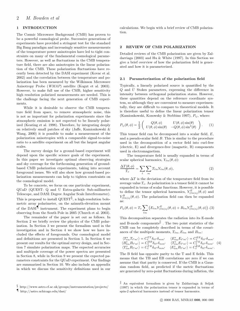
Figure 1. CMB temperature and polarization power spectra.The dashed lines are for a model with no re-ionization while thedotted lines are for a model with no gravitational lensing. Thesolid lines include the effects of both gravitational lensing andre-ionization. Model parameters are given in Section 5.

able to measure the polarization on such large angular scalesand so will not be sensitive to the effects of re-ionization.However, weak lensing affects the signal on small angularscales. CMB photons are deflected by the gravitational po-tential of large scale structure. For the TT and EE spectra,this effect results in a smearing of the acoustic peaks on largeangular scales, although the change to the spectra is verysmall, as shown in Fig. 1. However, lensing will also convertE-mode polarization into B-modes. This means that therewill be a scalar contribution to the B-mode spectrum dueto lensing. Therefore, the B-mode spectrum will be contam-inated by a GL contribution, the spectrum of which mustbe measured precisely so that it can be removed (Knox &Song 2002, Kesden, Cooray & Kamionkowski 2002). As thelensing signal peaks at small angular scales, ground-basedexperiments are well-suited to this task.

The lensing signal itself also contains useful informa-tion about large-scale structure. This can be used to con-strain other cosmological parameters such as the neutrinomass (Kaplinghat, Knox & Song 2003), since this will addto the mass-energy of the universe, altering its expansionhistory, and suppressing small scale power in the matterpower spectrum due to free streaming. The lensing signalwill also make the CMB sensitive to the equation of state ofthe universe, parameterized by w = p/ρ, as again this willaffect the expansion history.

Fig. 1 shows the temperature and polarization powerspectra, generated by the Boltzmann and Einstein solverCMBFAST (version 4.2; Seljak & Zaldarriaga (1996)⋆⋆,decomposed into temperature-temperature (TT) power,temperature-E-mode (TE) cross-power, E-mode-E-mode(EE) power, and B-mode-B-mode (BB) power. We plot spec-tra without gravitational lensing (dotted lines) and withoutre-ionization (dashed lines) and with both included (solid

⋆⋆ http://www.cmbfast.org/

c© 0000 RAS, MNRAS 000, 000–000

4 M. Bowden et al

lines). The main aim of this paper is to optimize the mea-surement of the polarization spectra. In the following sectionwe present our formalism for this optimization, based on theFisher Information matrix.

3 FORMALISM

3.1 Fisher Information matrix

For a model dependent on a set of parameters, α, the proba-bility of a particular parameter set, given a set of experimen-tal data points, d, is expressed by the likelihood function,L(α|d), the probability of the parameters given the data.By exploring the parameter space to maximize L we maydetermine the parameter values within certain error limits.The minimum possible variance with which a parameter canbe measured can be estimated from the Fisher informationmatrix (Tegmark, Taylor & Heavens 1997), defined as:

Fij =

⟨

∂2L∂αi∂αj

⟩

, (5)

where L = − lnL and the derivatives are evaluated at themaximum likelihood values of the parameters. The inverseof the Fisher matrix gives the parameter covariance matrix,Cij , for the theoretical parameters:

Cij ≡ 〈∆αi∆αj〉 = F−1ij , (6)

where ∆αi is the deviation of the parameter from its max-imum likelihood value. The diagonal of the inverse Fishermatrix yields the marginalized 1-σ error on the parameters.Taking the inverse of the diagonal of the Fisher matrix,

(∆αi)2 = 1/Fii, (7)

yields the conditional error on the parameters. In general

[F−1]ii ≥ 1/Fii, (8)

where the equality holds only for uncorrelated parameters.The Fisher matrix then provides a theoretical upper boundon the accuracy of a measurement of a given parameter fora given experiment.

3.2 Application of Fisher matrix to CMB

experiments

For a CMB experiment, the data are the measurements ofthe four CMB power spectra and the parameters are thecosmological parameters. For the measurement of a singlepower spectrum, Cℓ, the Fisher matrix is given by:

Fij =∑

ℓ

1

(∆Cℓ)2∂Cℓ∂αi

∂Cℓ∂αj

, (9)

where

(∆Cℓ)2 =

2

(2ℓ + 1)fsky∆ℓ(Cℓ + Nℓ)

2

is the error in the measurement of the power spectrum in aband centred on multipole ℓ, and Nℓ is a noise term. Thesurvey area is given by fsky . The summation is over pass-bands of width ∆ℓ.

For a measurement of all four power spectra this gen-eralizes to (Zaldarriaga & Seljak 1997):

Fij =∑

ℓ

∑

XY

∂CXℓ

∂αi[Ξℓ]

−1XY

∂CYℓ

∂αj, (10)

where X and Y are either TT, EE, TE or BB and ΞXY ≡Cov(CX

ℓ CYℓ ) is the power spectra covariance matrix:

Ξℓ =

ΞTT,TTℓ ΞTT,EEℓ ΞTT,TEℓ 0

ΞTT,EEℓ ΞEE,EEℓ ΞEE,TEℓ 0

ΞTT,TEℓ ΞEE,TEℓ ΞTE,TEℓ 0

0 0 0 ΞBB,BBℓ

. (11)

The terms in the power spectra covariance matrix are givenby:

Ξxy,x′y′

ℓ =1

(2ℓ + 1)fsky∆ℓ

×[

(Cxy′

ℓ + Nxy′

ℓ )(Cyx′

ℓ + Nyx′

ℓ )

+(Cxx′

ℓ + Nxx′

ℓ )(Cyy′

ℓ + Nyy′

ℓ )]

, (12)

where (x, y) = (T, E, B). The noise covariance is given byNxyℓ . In the case of no foregrounds this is given by:

Nxyℓ = w−1

x |Bxℓ |−2δxy, (13)

where, w−1x = Ωxpix(σ

xpix)

2, for an experiment with solidangle per pixel, Ωpix, and the noise per pixel, σpix. Thepixel noise depends on survey design and instrument pa-rameters. For an experiment covering an area Θ2 for an in-tegration time tobs, with NPSB detectors, beam size θ and a

sensitivity††, NET, the pixel noise is:

σ2pix =

NET2Θ2

tobsNPSBθ2B

. (14)

In Section 4 we discuss how the noise terms may be extendedto include foregrounds. The spherical harmonic transform ofthe beam is given by Bℓ. Here we assume that the beam isa Gaussian,

Bℓ = exp(

−ℓ(ℓ + 1)σ2B/2)

, (15)

with σB = θB/√

8 ln 2 where θB is the full width half maxi-mum beam size.

The minimum resolution of the power spectra, ∆ℓ, de-pends on the area of sky covered, ∆ℓ = 360/Θ. This willtherefore also give the minimum ℓ at which the power spec-tra can be measured as discussed further in Section 6.2. Ifa resolution smaller than this is used, the different ℓ modeswill become correlated and equation (4) will no longer ap-ply (Hobson & Magueijo 1996). We calculate the maximumℓ value from the FWHM beam size, ℓmax = π/θ. In reality,multipoles higher than this could be measured if the beamprofiles can be accurately determined.

The Fisher matrix also provides a simple way to cal-culate the results obtainable by combining a number of ob-servations from different CMB experiments. In the simplestcase, in which Nexp experiments observe different patchesof sky, the combined Fisher matrix, FC , is the sum of theindividual Fisher matrices, Fe (Hu 2001):

FCij =

Nexp∑

e

Feij . (16)

†† The definition of sensitivity for a polarization experiment isdiscussed in Appendix (A).

c© 0000 RAS, MNRAS 000, 000–000

Optimization of a ground-based CMB polarization experiment 5

If any of the patches of sky overlap, each overlapping regionis considered as a separate patch. In these patches the com-bined noise covariance, Nℓ, of the overlapping experimentsshould be used to calculate the terms in the power spectracovariance matrix (equation (12)). This is discussed furtherin the next section where we consider how to optimally com-bine multi-frequency data.

This completes the formal machinery we will requirefor our analysis. Note that we have ignored the effects ofwindowing and mode-mixing due to limited sky coverage(e.g. Bunn 2002), and non-Gaussianity and mode-couplinginduced by gravitational lensing (e.g. Guzik, Seljak & Zal-darriaga 1999). The former effects modes by convolvingthem with the survey window function and mixing E andB modes. This will mainly effect the B-modes, where thesignal-to-noise is poor, and will slightly increase our uncer-tainties. Non-Gaussianity induced by gravitational lensingwill also correlate modes and will give rise to higher-ordercorrelations, which will also lead to a slight increase in ouruncertainties.

So far we have also ignored the effects of foregroundcontamination, and it is to this we now turn.

4 FOREGROUNDS

4.1 Including foregrounds into the formalism

The signal measured from the sky will contain not only acomponent from the CMB, but also a contribution fromastrophysical foregrounds. The CMB signal is independentof the wavelength of the observation, but the signal frommost foregrounds is expected to be frequency dependent.By observing in a number of different frequency channelsit is therefore possible to reduce the total foreground con-tamination by optimally combining the signal from differentfrequency channels. It may also be possible to use the multi-ple frequency information to remove some of the foregroundcontamination from the signal (e.g. Maino et al. 2002, Hob-son et al. 1998).

The effect of observing over multiple channels needs tobe taken into account in the Fisher matrix formalism de-scribed in the previous Section. If we ignore foregrounds andconsider only detector noise, we can simply replace the noiseterms in equation (12) by an inverse variance weighting ofthe noise in each channel, Nℓ,c:

Nℓ =

(

∑

f

1

Nℓ,f

)−1

. (17)

By choosing this weighting scheme at each multipole wecombine the signals by giving the most weight to the chan-nels with the smallest detector noise.

We include the effect of foregrounds by treating the fore-grounds as an extra source of noise with power spectra Nfg

ℓ

for each different power spectra in each frequency channel.This gives us the maximum possible foreground contamina-tion i.e. the contamination assuming that no foreground re-moval will be attempted. However, unlike the detector noise,the foregrounds will be correlated between power spectraand between frequency channels. To include these correla-tions we follow the technique developed in Tegmark et al.(2000, hereafter T00). We define a 3F × 3F noise matrix,

Nℓ, for each multipole, where F is the number of frequencychannels in the experiment:

Nℓ =

NTTℓ NTE

ℓ 0NTEℓ NEE

ℓ 00 0 NBB

ℓ

, (18)

where each component of this matrix, NXX′

ℓ , is an F × Fmatrix giving the variances and covariances of the noise inthe F channels. Each element in Nℓ is the sum of the con-tribution from each of the possible foregrounds, NXX′

ℓ(k) and

the detector noise, NXX′

ℓ(det):

NXX′

ℓ = NXX′

ℓ(det) +∑

k

NXX′

ℓ(k) , (19)

where the sum over k is a sum over each of possible fore-grounds which could contribute to the signal. We define the3F × 3 scan matrix, A, where:

A =

(

e 0 00 e 00 0 e

)

, (20)

and e is a column vector of height F consisting entirely ofones. If F = 2 as would be the case for QUaD (see Section6.2) then:

A =

1 0 01 0 00 1 00 1 00 0 10 0 1

. (21)

The weighted noise for each polarization is then obtained bycalculating the 3 × 3 covariance matrix, Σℓ, where:

Σℓ =(

AtNℓA

)−1=

NTTℓ NTE

ℓ 0

NTEℓ NEE

ℓ 00 0 NBB

ℓ

. (22)

The terms, NXXℓ are now the noise terms used in equation

(12) to calculate the power spectra covariance matrix. If thenoise is not correlated between T and E and not correlatedbetween channels (as is the case if we include only detectornoise) then Nℓ becomes diagonal and the procedure is iden-tical to the minimum variance weighting of equation (17).

In the last section we discussed how to combine a num-ber of experiments by adding the Fisher matrices of inde-pendent patches of sky. For patches in which a number ofexperiments overlap, the required noise term, Nℓ, can becalculated by considering a single experiment with chan-nels at each of the different frequencies used by this set ofexperiments. For this patch F will then become the totalnumber of frequency channels in the combined survey. Ifany of the instruments used have channels which cannotmeasure either temperature or polarization, then rows andcolumns corresponding to these channels should be removedfrom the full noise matrix, Nℓ and from the scan matrix,A, in the relevant places. For example, QUaD would not beable to measure temperature information (see Section 6.2).If we combine the two QUaD channels with another exper-iment measuring both temperature and polarization, thesetwo channels should be removed from the first row and firstcolumn of the matrix Nℓ in equation (18) and the size of

c© 0000 RAS, MNRAS 000, 000–000

6 M. Bowden et al

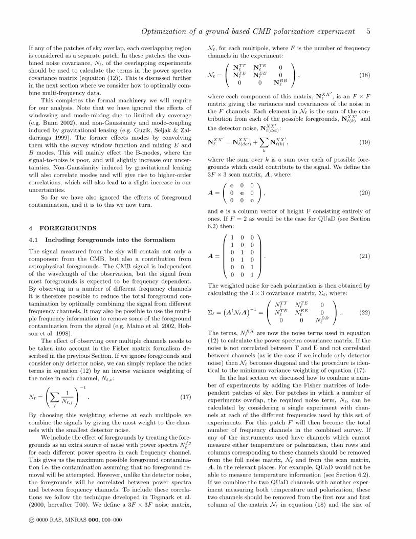
Figure 2. Models used for vibrating dust, synchroton emissionand residual point sources (black) compared to the EE and BBpower spectra (light grey, solid). The different lines show fore-ground models at 100 GHz (dash-dot) and 150 GHz (dash). Thetotal foreground power spectra are also shown on each plot (darkgrey). The GW component of the BB-spectra is shown for r = 0.1(upper dotted line) and r = 0.01 (lower dotted line). The otherforegrounds are either unpolarized or can be neglected

the vector e in the first column of the matrix A in equation(20) should be reduced.

4.2 Foreground models

We closely follow T00 in constructing the foreground powerspectra required in the previous section, and use the software

provided on the associated website ‡‡. QUaD proposes to ob-serve at frequencies of 100 and 150 GHz. At these frequen-cies the relevant foregrounds are diffuse free-free emission,IR and radio point sources, synchrotron radiation and vi-brating dust, rotating dust and thermal Sunyaev-Zeldovich(SZ) radiation. Each foreground is modelled using a spatialpower spectrum, Cl (k) = (pA)2 l−β where p is the frac-tion polarized and A is the overall amplitude. A frequencydependence is also defined and normalized to unity at a ref-erence frequency, ν∗. For point sources it is assumed thatvery bright sources (5 σ outlyers) will be removed from theCMB maps, but that there will still be a residual pointsource contamination after this subtraction. In T00, setsof estimates for these parameters are given. We begin byusing their “middle-of-the-road” foreground model. In thismodel, the only polarized foregrounds are sychrotron, dustand point sources. However, recent observations (Kovac etal. 2002; Bennett et al. 2003, hereafter B03) have shown theamplitudes of the foregrounds in these models to be overlypessimistic. We have therefore lowered the amplitudes of vi-brating dust and synchrotron radiation to match roughlythose given in Fig. 10 of B03. Also following B03 we havelowered the amplitude of the radio point sources and have

‡‡ http://www.hep.upenn.edu/∼max/foregrounds.html

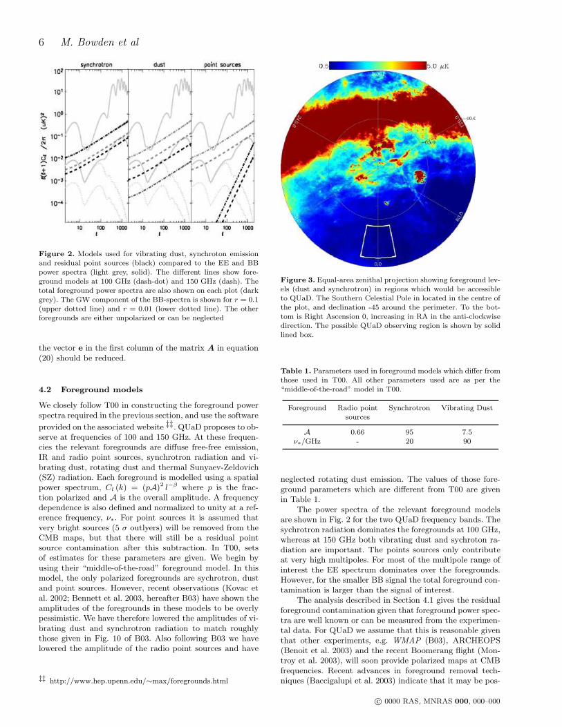
Figure 3. Equal-area zenithal projection showing foreground lev-els (dust and synchrotron) in regions which would be accessibleto QUaD. The Southern Celestial Pole in located in the centre ofthe plot, and declination -45 around the perimeter. To the bot-tom is Right Ascension 0, increasing in RA in the anti-clockwisedirection. The possible QUaD observing region is shown by solidlined box.

Table 1. Parameters used in foreground models which differ fromthose used in T00. All other parameters used are as per the“middle-of-the-road” model in T00.

Foreground Radio point Synchrotron Vibrating Dustsources

A 0.66 95 7.5ν∗/GHz - 20 90

neglected rotating dust emission. The values of those fore-ground parameters which are different from T00 are givenin Table 1.

The power spectra of the relevant foreground modelsare shown in Fig. 2 for the two QUaD frequency bands. Thesychrotron radiation dominates the foregrounds at 100 GHz,whereas at 150 GHz both vibrating dust and sychroton ra-diation are important. The points sources only contributeat very high multipoles. For most of the multipole range ofinterest the EE spectrum dominates over the foregrounds.However, for the smaller BB signal the total foreground con-tamination is larger than the signal of interest.

The analysis described in Section 4.1 gives the residualforeground contamination given that foreground power spec-tra are well known or can be measured from the experimen-tal data. For QUaD we assume that this is reasonable giventhat other experiments, e.g. WMAP (B03), ARCHEOPS(Benoit et al. 2003) and the recent Boomerang flight (Mon-troy et al. 2003), will soon provide polarized maps at CMBfrequencies. Recent advances in foreground removal tech-niques (Baccigalupi et al. 2003) indicate that it may be pos-

c© 0000 RAS, MNRAS 000, 000–000

Optimization of a ground-based CMB polarization experiment 7

sible to remove some of the foreground noise from the signal.The residual foreground contamination used here thereforegives an upper limit on that which can be expected in thefinal cleaned maps, given that our foreground models areaccurate.

For a ground-based experiment it will also be possibleto select preferentially regions of sky to observe in whichthe foreground fluctuations are small, and so the foregroundnoise can be reduced further. Fig. 3 shows the region of skywhich would be accessible to QUaD from the South Pole andthe estimated levels of foreground contamination across thisarea from dust (Finkbeiner, Davis & Schlegel 1999) and syn-chroton (Giardino et al. 2002) using the modified foregroundmodels. A possible observing patch for QUaD is also shownin which the mean foreground amplitude is low. However, amore detailed analysis will be performed to choose the finalobserving patch with the lowest possible foreground vari-ance across the mutipole range of interest. For these reasonswe perform the relevant calculations once using the full-skyforeground models descibed here, and again assuming thatthe foregrounds are negigible.

We conclude that while our current understand of po-larized foregrounds is evolving, the expected level of fore-ground contamination in the EE power spectrum should notbe significant. The GL component of the BB power spec-trum should also be detectable if patches of sky with lowforeground variance can be targeted or if foreground removaltechniques can be successfully implemented. This would alsomean that the GW B-mode component should be measure-able if the tensor-to-scalar ratio is large.

5 COSMOLOGICAL MODEL

In order to calculate the terms in the power spectrum covari-ance matrix and the power spectrum derivative we require amodel from which to calculate the CMB power spectra. Thismodel is defined by two sets of parameters: the inflation-ary parameters which parameterize the initial perturbationscausing the fluctuations in the CMB, and the cosmologicalparameters which determine how these initial perturbationsare propagated into the observed CMB power spectra. Givena set of parameters, the CMB power spectra can then becalculated using a Boltzmann and Einstein solver. For thiswork we have used a slightly modified version of CMBFASTv4.2.

The initial scalar perturbations are parameterized by:

∆2R(k) = ∆2

R(k0)(

k

k0

)ns−1

, (23)

where ∆2R(k) is the power spectra of R, the curvature per-

turbation in the comoving gauge, and ns is the slope of thescalar power spectrum. The tensor perturbations are givenby:

∆2T (k) = ∆2

T (k0)(

k

k0

)nt

, (24)

where ∆2T (k) is the power spectra of gravitational waves

from inflation and nt is the slope of the gravitational wavepower spectrum. The amplitude terms are evaluated at thepivot wave number, k0 = 0.05Mpc−1. To parameterize theinitial perturbations we use three inflationary parameters:

A, a constant of order unity which is proportional to theamplitude of the initial scalar perturbations, ns, the tilt ofthe power spectra of the initial scalar perturbations and r,the ratio of tensor to scalar perturbations. These are theparameters used in the analysis of the WMAP data (Spergelet al. 2003). We do not consider here the running of thespectral index, n′

s. The exact relationship between A and∆2

R(k0) is derived in Verde et al (2003; equation (32)). Thetensor-to-scalar ratio is defined as:

r =∆2T (k0)

∆2R

(k0). (25)

Note that a number of different definitions are used in theliterature. The most common alternatives are to define r interms of the Newtonian potential:

rψ =∆2T (k0)

∆2ψ(k0)

, (26)

so that rψ ≃ (5/3)2r, or in terms of the CMB radiationquadrupoles:

rQ =CT

2

CS2

. (27)

The relation between r and rQ depends on the cosmologicalparameters used in the model (Turner & White 1996).

The cosmological parameters we shall consider areΩbh2, Ωmh2, h, τ, where h is the Hubble constant in unitsof 100 kms−1Mpc−1, Ωb is the energy density of baryons,Ωm is the total matter density and τ is the optical depth tothe last scattering surface. Again, these are the parameterschosen for the WMAP data analysis (Verde et al. 2003). Thefull set of parameters, and their best-fit values from WMAP

(Spergel et al. 2003), is then:

Ωbh2, Ωmh2, h, τ, ns, r, A =

0.0224, 0.135, 0.71, 0.17, 0.93, 0.01, 0.83.For this parameter set the relation between the r and rQis approximately rQ ≈ 2.8r and ∆2

R(k0) = 2.45 × 10−9.The values of these parameters are taken from the best fitWMAP model (Spergel et al. 2003) except for r, which can-not be well constrained by this data set. The current up-

per limit on r is about 0.36 (Leach & Liddle 2003)§§. Thelowest possible r which can be detected is of the order of10−4 (Knox & Song 2002, Kesden, Cooray & Kamionkowski2002) due to noise left over from the removal of the gravita-tional lensing signal from the B-mode spectrum. To reflectthis range of possible values we perform the calculations,which have strong dependence on r, at two different values,r = 0.01 and r = 0.1.

6 SURVEY OPTIMIZATION

6.1 Method

The optimization of the survey area for a ground based mea-surement of the CMB polarization has been addressed previ-ously (Jaffe et al. 2000) in the context of making a detection.

§§ Note that our value differs from the value given in this refer-ence as we use a different value for the pivot wavenumber, k0

c© 0000 RAS, MNRAS 000, 000–000

8 M. Bowden et al

We extend this work by considering the criteria for an op-timal measurement of the polarization spectra, for a fixedobserving time, with the new generation of ground based in-struments. We also include the effects of gravitational lens-ing and foregrounds.

The main aim of a polarization experiment is to makemeasurements of the three polarization power spectra, CTE

ℓ ,CEEℓ and CBB

ℓ , with the highest possible precision, withina prescribed timescale. The error in the measurement of thepower spectra is determined by two conflicting factors. Fora fixed total observing time, the integration time per unitarea (or pixel) is inversely proportional to the total area; asmaller map will therefore result in a lower pixel noise. How-ever, for a smaller map there are fewer independent modesfrom which to measure each multipole (i.e. the averaging inequation (4) will be made over fewer values of m) and so thesample variance will increase.

To quantify these effects, we choose a single parameterfor which to evaluate the Fisher matrix, AX , the amplitudeof each power spectrum. For a single parameter the variancein the measurement of this parameter, (∆AX)2, is then givenby 1/FAXAX . From equation (9) the error in AX is:

(∆AX)2 =

(

∑

ℓ

1

(∆CXℓ )2

(CXℓ )2

(AX)2

)−1

, (28)

where (∆CXℓ )2 for each power spectrum are given by the

diagonal elements of the power spectrum covariance matrixin equation (11). We then define a figure of merit parameteras the signal to noise ratio in the measurement of each powerspectrum, SNR, which is given by:

SNR =

(

AX

∆AX

)

=

√

√

√

√

∑

ℓ

(

CXℓ

∆CXℓ

)2

. (29)

To find the optimal area for a measurement of each powerspectrum we therefore need to find the area which givesthe highest SNR subject to the constraint of a fixed totalobserving time. Here we shall assume that our survey willlast 24 months and normalize the timescale for the surveyto a known area that could be scanned in this time.

This optimization procedure could be done for any pa-rameter, or combination of parameters. However for simplic-ity, and as a prerequisite to the measurement of the polar-ization power spectra, we will maximize the SNR for theamplitude. In principle, other parameters for the survey ortelescope could be left free, such as the pixels size or beamwidth. In practice we find that the smallest pixel/beam sizeis preferred, and so we set this to the limit of a given exper-iment.

6.2 QUaD instrument parameters

As a specific example of a ground-based experiment we usethe QUaD experiment. This enables us to fix the instrumentparameters needed to determine the pixel noise (equation14) and the allowed multipole range. These parameters aregiven in Table 2. A detailed description of QUaD is given inChurch et al. (2003).

The maximum multipole which can be covered is lim-ited by the beamsize as discussed in Section 3. If no other

Table 2. Expected QUaD instrument parameters

Frequency (GHz) 100 150Number of bolometers 24 38Angular resolution (arcmin) 6.3 4.2

NET per bolometera (µKs1/2) 270 300

a - The definition of sensitvity for a polarization sensitive bolome-ter is discussed in Appendix A.

effect needs to be taken into consideration the minimummultipole, ℓmin, would be determined from the survey area,ℓmin = 360/Θ. However, for a ground-based experimentthe lower-ℓ cut-off is also limited by the stability of the at-mosphere. This will limit the maximum scan which can beused and hence the largest angle on the sky over which acorrelation can be made. For a perfect polarization experi-ment, this would not be an issue, as the unpolarized atmo-spheric fluctuaions would not be detected in the polarizeddata. However, instrumental effects will cause a fraction ofthe unpolarized (common mode) signal to be to be presentin the polarized signal. The atmosphere at the South Pole isexceptionally stable (Halverson & Lay 1998) and the QUaDinstrument has been designed is such a way that these ef-fects will be minimized, so we estimate that a minimum ℓof 25 can be reached. The minimum ℓ used in equation (29)will then be ℓmin = max(360/Θ, 25). Although it is possi-ble for QUaD to make total power measurements, there isno mechanism for removing the atmospheric noise from theresulting data and so we assume that QUaD would not beable to produce temperature maps.

We estimate the total observing time by assuming thatQUaD will observe at the South Pole only in the austral win-ter (six months) for 22 hours each day and assuming that 20per cent of this total time will be lost due to bad weather,instrument maintenance and calibration time. These esti-mates are based on the experiences of the DASI team at theSouth Pole site (Kovac et al. 2002). This gives a total timespent observing on the CMB of 3210 hours per year. Themaximum useable patch of sky is about 1000 deg2, limitedby available sky visible from the survey site, and major fore-ground contamination from the Galactic plane (see Fig. 3).We therefore restrict the analysis to areas below this maxi-mum survey size.

It is important to note that to measure both the Q andU Stokes parameters, each pixel must be measured with thedetector in at least two different orientations with respectto the sky. For QUaD this will be achieved by rotating ahalf-wave plate so that both Q and U can be measured byeach detector. This halves the total integration time avail-able for each Stokes parameter when making a polarizedmeasurement.

6.3 Results

We have applied the above procedure to a model QUaDexperiment. We consider three different cases:

(i) a measurement of the EE spectrum,(ii) a measurement of the BB spectrum including the lens-

ing component as part of the signal we wish to measure,

c© 0000 RAS, MNRAS 000, 000–000

Optimization of a ground-based CMB polarization experiment 9

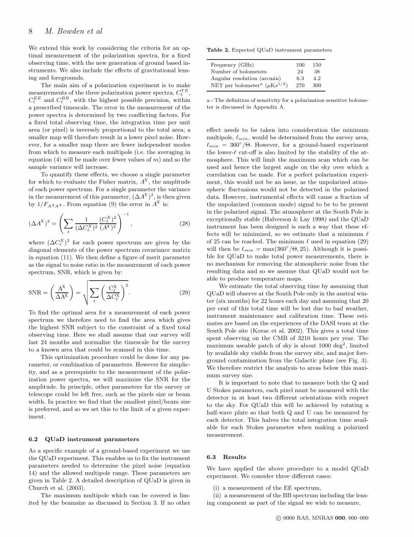
Figure 4. Variation of SNR with survey area for the EE (left)and total BB (right) power spectra with foregrounds (solid lines)and without foregrounds (dashed lines) for an observing time of1 year (light) and 2 years (dark) for r=0.01

(iii) a measurement of just the BB GW spectrum includ-ing the lensing signal as an extra source of noise.

The results for the optimization of a 24-month ground-based survey are presented in Table 3, for TE, EE andBB spectra, for the case of foregrounds, and without fore-grounds. The latter is of interest if the foregrounds are wellenough understood to be subtracted from the signal or if apatch of sky with very low foreground variance can be found,as discussed in Section 4

Fig. 4 shows how the SNR varies with area for EE andBB spectra. From Fig. 4 (left) it can be seen that a ground-based polarization experiment can make a good measure-ment of the EE spectrum, even if the foreground contami-nation is not well understood. The SNR is close to 100 forsurvey areas over 300 deg2. Below this size the SNR fallsrapidly to zero. For an experiment with the sensitivity andmultipole coverage of QUaD, an E-mode survey is sample-variance-limited, so that a larger area is preferable (> 1000deg2) for statistical purposes. Given that an E-survey willhave high signal-to-noise per pixel, a high-resolution polar-ization map of the surveyed area is also possible (see Section7), allowing for removal of point sources as discussed in Sec-tion 4.

Fig. 4 (right) shows the SNR for a two-year B-modesurvey. The dotted line is for a SNR=3 which is the min-imum SNR that can be considered as an actual detectionof the signal. Unlike the E-mode survey, the B-mode sur-vey is detector noise limited as the signal is much lower.With foregrounds the SNR sharply peaks at SNR ≈ 5.5 formuch smaller areas, around 50 deg2, where the lensing sig-nal dominates. As the survey area increases the noise perpixel increases and the overall SNR drops. If we can removeforeground contamination then the maximum SNR increasesto a value of 9 and the optimal area is slightly reduced, asshown in Table 3.

This different behaviour between the E and B-mode sur-veys with increasing area makes the simultaneous optimiza-tion of both measurements difficult. One compromise is touse the break in SNR of the E-mode survey at around 300deg2. Although this is sub-optimal for both surveys, the dropto SNR = 90 for the E-survey is minimal and SNR = 4.5 forthe B-mode survey is still a strong detection. An alternativewould be to split the survey in two, one large, one small,halving the integration time for each survey. As shown inFig. 4 for a single year of integration it is still possible todetect the B-mode signal if we concentrate on a small areaof sky (∼ 20 deg2). For a single year the EE SNR also doesnot drop significantly if an area larger than about 500 deg2

is chosen.

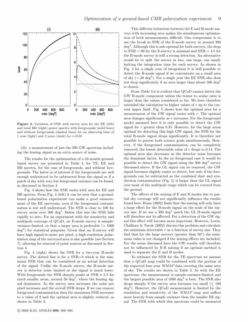
From Table 3 it is evident that QUaD cannot detect theGW B-mode component unless the tensor to scalar ratio islarger than the values considered so far. We have thereforeextended the calculation to higher values of r up to the cur-rent upper limit. Fig. 5 shows how the optimal area for ameasurement of the GW signal varies with r. The optimalarea changes significantly as r increases. For the foregroundmodel assumed here it is only possible to detect the GWsignal for r greater than 0.35. However, for the large areasoptimal for detecting this high GW signal, the SNR for thetotal B-mode signal drops significantly. It is therefore notpossible to pursue both science goals simultaneously. How-ever, if the foreground comtamination can be completelyremoved, the lowest detectable value of r drops to 0.14. Theoptimal area also decreases as the detector noise becomesthe dominant factor. In the no foreground case it would bepossible to detect the GW signal using the 300 deg2 surveydiscussed above. If the GL signal can be removed, the GWsignal becomes slightly easier to detect, but only if the fore-grounds can be subtracted as the combined dust and syn-chroton contamination (Fig. 2) is larger than the GL signalover most of the multipole range which can be covered fromthe ground.

The effects of the mixing of E and B modes due to par-tial sky coverage will not significantly influence the resultsfound here. Bunn (2002) finds that the mixing will only havea large effect for the B-mode signal on the scale of the sur-vey size. If we use a 300 deg2 patch the GL B-mode signalwill therefore not be affected. For a detection of the GW sig-nal this effect will become more important. However, Lewis,Challinor & Turok (2002) discuss this problem and calculatethe minimum detectable r as a function of survey size. Theyfind that for the large surveys (greater than 50) the mini-mum value is not changed if the mixing effects are included.For the areas discussed here the GW results will thereforenot be influenced by E-B mixing if an optimal method isused to separate the E and B modes.

To estimate the SNR for the TE spectrum we assumethat a QUaD map could be combined with the portion ofthe expected four-year WMAP data covering the same areaof sky. The results are shown in Table 3. As with the EEspectrum, the measurement is sample-variance-limited andthe largest possible area of 1000 deg2 is best. The SNR alsodrops sharply if the survey area becomes too small (≤ 100deg2). However, the QUaD measurement is limited by theresolution and sensitivity of the WMAP map and suffersmore heavily from sample variance than the smaller EE sig-nal. The SNR with which this spectrum could be measured

c© 0000 RAS, MNRAS 000, 000–000

10 M. Bowden et al

Figure 5. Variation of the survey optimal area (upper plot) andachievable SNR (lower plot) for a measurement of the GW sig-nal as a function of r with (solid line) and with (dashed line)foregrounds.

Table 3. SNRs for the optimal survey areas for each of the powerspectra for a two-year integration time with QUaD

Spectrum TE EE BB GWr 0.01 0.01 0.01 0.1 0.01 0.1

areaa /deg2 1000+ 1000+ 46 50 813 1000+areab /deg2 1000+ 1000+ 24 26 126 247

SNRa 31 118 5.6 5.7 0.1 1.0SNRb 31 119 9 9 0.4 2.5

a - including astrophysical foregroundsb - without astrophysical foregrounds

by QUaD is therefore smaller than the EE SNR. The TEspectrum has also already been measured in this multipolerange by WMAP. It is therefore more useful to optimize aground-based survey for a measurement of the EE and BBspectra.

We have also investigated the effect of increasing theminimum ℓ value used in the optimization. For the TE, EEand total BB spectra, an increase in the minimum ℓ from 25to 100 has a negligible effect, as most of the power in thesespectra is from the higher multipoles. However, as would beexpected, increasing the minimum ℓ does affect the GW B-mode detection. If the minimum ℓ is increased to 100 theGW is no longer detectable below the current upper limit of0.36.

7 DEEP MAPS OF THE CMB POLARIZATION

For a ground-based experiment it is not possible to make ob-servations of the whole sky due to the limited sky coverageavailable from the ground. Although this is a disadvantagein terms of multipole coverage at low ℓ, by making a deep in-tegration of a small region of sky it is possible to make mapswith a very high signal-to-noise ratio. This allows more pre-

Table 4. Planck and WMAP instrument parameters. For WMAP

we use only the highest two frequency channels as the other chan-nels are used mainly to constrain foreground contributions.

Planck WMAP

frequency /GHz 40 70 150 220 70 90

NET /µKs1/2 220 300 80 120 1521 2071Beam size /arcmin 24 14 7 5 20 13Detector number 6 12 8 8 8 16

cise measurements to be made on small angular scales. Itwill also improve the ability of the experiment to removelow-lying systematic effects which would not be detectablein observations of lower signal-to-noise. We illustrate the dif-

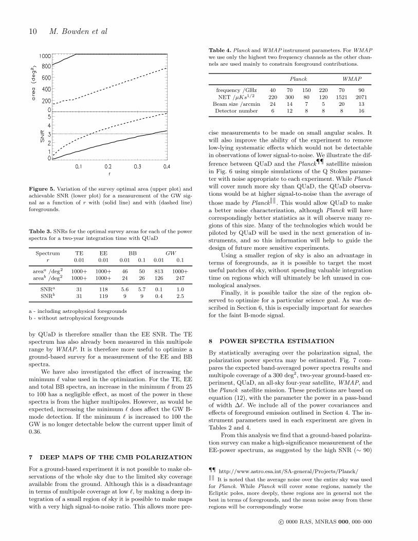
ference between QUaD and the Planck¶¶ satelllite missionin Fig. 6 using simple simulations of the Q Stokes parame-ter with noise appropriate to each experiment. While Planck

will cover much more sky than QUaD, the QUaD observa-tions would be at higher signal-to-noise than the average of

those made by Planck‖‖. This would allow QUaD to makea better noise characterization, although Planck will havecorrespondingly better statistics as it will observe many re-gions of this size. Many of the technologies which would bepiloted by QUaD will be used in the next generation of in-struments, and so this information will help to guide thedesign of future more sensitive experiments.

Using a smaller region of sky is also an advantage interms of foregrounds, as it is possible to target the mostuseful patches of sky, without spending valuable integrationtime on regions which will ultimately be left unused in cos-mological analyses.

Finally, it is possible tailor the size of the region ob-served to optimize for a particular science goal. As was de-scribed in Section 6, this is especially important for searchesfor the faint B-mode signal.

8 POWER SPECTRA ESTIMATION

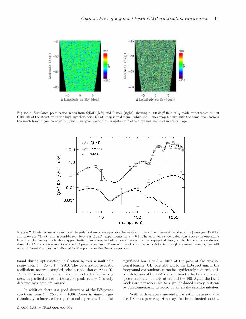
By statistically averaging over the polarization signal, thepolarization power spectra may be estimated. Fig. 7 com-pares the expected band-averaged power spectra results andmultipole coverage of a 300 deg2, two-year ground-based ex-periment, QUaD, an all-sky four-year satellite, WMAP, andthe Planck satellite mission. These predictions are based onequation (12), with the parameter the power in a pass-bandof width ∆ℓ. We include all of the power covariances andeffects of foreground emission outlined in Section 4. The in-strument parameters used in each experiment are given inTables 2 and 4.

From this analysis we find that a ground-based polariza-tion survey can make a high-significance measurement of theEE-power spectrum, as suggested by the high SNR (∼ 90)

¶¶ http://www.astro.esa.int/SA-general/Projects/Planck/‖‖ It is noted that the average noise over the entire sky was usedfor Planck. While Planck will cover some regions, namely theEcliptic poles, more deeply, these regions are in general not thebest in terms of foregrounds, and the mean noise away from theseregions will be correspondingly worse

c© 0000 RAS, MNRAS 000, 000–000

Optimization of a ground-based CMB polarization experiment 11

Figure 6. Simulated polarization maps from QUaD (left) and Planck (right), showing a 300 deg2 field of Q-mode anisotropies at 150GHz. All of the structure in the high signal-to-noise QUaD map is real signal, while the Planck map (shown with the same pixelization)has much lower signal-to-noise per pixel. Foregrounds and other systematic effects are not included in either map.

Figure 7. Predicted measurements of the polarization power spectra achievable with the current generation of satellite (four-year WMAP

and two-year Planck) and ground-based (two-year QUaD) experiments for r = 0.1. The error bars show detections above the one-sigmalevel and the free symbols show upper limits. The errors include a contribution from astrophysical foregrounds. For clarity we do notshow the Planck measurements of the EE power spectrum. These will be of a similar sensitivity to the QUaD measurements, but willcover different ℓ ranges, as indicated by the points on the B-mode spectrum.

found during optimization in Section 6, over a multipolerange from ℓ = 25 to ℓ = 2500. The polarization acousticoscillations are well sampled, with a resolution of ∆ℓ ≈ 20.The lower modes are not sampled due to the limited surveyarea. In particular the re-ionization peak at ℓ = 7 is onlydetected by a satellite mission.

In addition there is a good detection of the BB-powerspectrum from ℓ = 25 to ℓ = 1000. Power is binned loga-rithmically to increase the signal-to-noise per bin. The most

significant bin is at ℓ = 1000, at the peak of the gravita-tional lensing (GL) contribution to the BB-spectrum. If theforeground contamination can be significantly reduced, a di-rect detection of the GW contribution to the B-mode powerspectrum could be made at around ℓ = 100. Again the low-ℓmodes are not accessible to a ground-based survey, but canbe complementarily detected by an all-sky satellite mission.

With both temperature and polarization data availablethe TE-cross power spectra may also be estimated so that

c© 0000 RAS, MNRAS 000, 000–000

12 M. Bowden et al

a cross-check can be made with other measurements of thissignal.

With such high-resolution polarization informationavailable it is interesting to see what effect a ground-basedsurvey will have on cosmological parameters.

9 PARAMETER ESTIMATION

In this Section we investigate the contribution which canbe made by ground-based polarization experiments to themeasurement of the cosmological parameters. Previous workon CMB parameter estimation (Efstathiou & Bond 1999;Zaldarriaga, Spergel & Seljak 1997; Bond, Efstathiou &Tegmark 1997) has shown that the polarization data whichcan by obtained by the forthcoming WMAP and Planck

satellite missions will allow a more accurate determinationof many of the key cosmological parameters. For a satelliteexperiment, this is mainly because the degeneracy betweenτ and A can be broken by measuring the re-ionization bumpin the polarization power spectra. These re-ionization bumpsalso create a high GW B-mode signal at low ℓ, so a full-skymeasurement will also tighten constraints on the tensor-to-scalar ratio.

As we have discussed, a ground-based polarization ex-periment can concentrate on smaller areas of sky at higherresolution and so can make a good measurement of theacoustic peaks out to high ℓ in the EE-power spectrum. Theinformation from a ground-based experiment will thereforecomplement the full-sky satellite data. It is also possibleto choose an observing strategy with targets the GW sig-nal peak at intermediate scales (ℓ = 100). Ground-basedconstraints on the B-mode GW signal will therefore alsocomplement those obtainable from the current generationof satellite experiments.

Finally, it is important to note that a CMB polarizationexperiment is not just adding more data. A similar exper-iment measuring only the temperature spectrum, over thesame multipole range, and with the same detector sensitiv-ity, would add very little new information as far as cosmo-logical parameters are concerned, although a high-ℓ tem-perature surveys may well start to probe higher-order CMBeffects. Hence polarization adds unique information from theCMB.

We investigate the potential increase in the precisionof the measurement of cosmological parameters which canbe achieved with a ground-based experiment by comparingthe expected four-year results from WMAP alone to thosewhich could be achieved by combining QUaD and WMAP

data. To compare the two cases we calculate the inverseFisher matrix using equation (10) to find the variances andcovariances between each of the parameters. For QUaD weuse the instrument model dicussed in Section 6.2. The ex-perimental parameters used for WMAP are given in Table4.

To calculate the derivatives in parameter space requiredin equation (10) we use second-order differencing betweenCMBFAST models for accuracy, with the corresponding pa-rameter changed up and down by 1 per cent. The deriva-tive of the power spectrum encapsulates the response of thespectrum to a change in a particular parameter and hencequantifies its information content. However, if the shape of

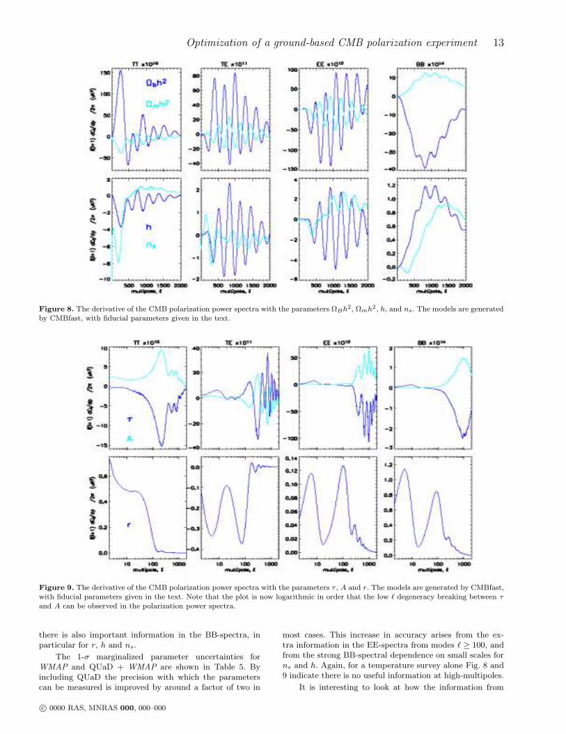
the derivative for any two parameters is too similar then thetwo parameters will be degenerate and cannot both be con-strained. The derivatives used in the calculation are shownin Fig. 8 and 9. For most parameters, the shape of the deriva-tives reflects the acoustic peaks in the power spectrum, in-dicating that both information about parameters and theirdifferences are contained in the peaks. For instance withtemperature only Ωmh2 and ΩBh2 are quite anti-correlated,but their derivatives oscillate out of phase for TE and EE-spectra, breaking this degeneracy. Much of the differencebetween h and ns occurs in the low multipoles, but thereis a large difference at high-ℓ in the BB-spectra due to theeffects of gravitational lensing on these modes.

Fig. 9 clearly shows the anti-correlation that arises be-tween τ and A when only temperature information is avail-able. This degeneracy is seen to be broken on large scalesby the differences in the responses of the polarization powerspectra. However, going to high ℓ in the polarization spec-tra, these parameters become strongly degenerate again.Hence we can expect that a ground-based polarization sur-vey, which will have difficulty reaching the lower multipolerange, will not contribute much to lifting the A− τ degener-acy. Conversely, with only temperature information, h andns are strongly degenerate, with much of the difference inresponse coming at very low modes, or modes beyond a fewhundred. However, adding polarization information, espe-cially TE at around ℓ of 100, and lensed BB modes at highℓ, breaks this degeneracy due to their different responses

Finally with only a temperature spectrum, the responseto r is limited to the first hundred multipoles. The TE andEE derivatives show that there is useful information aboutr on intermediate scales in the polarization spectra up toaround ℓ = 500, but for these multipoles the scalar EE andTE power spectra are very high and so it will be difficult toextract this information from the signal. However, the BBderivative also shows structure at higher multipoles and willprovide information on r if the tensor signal is higher thanthe scalar lensing signal at the scales of interest, or if thelensing signal can be removed.

Having considered the responses of the power spectra toour parameter set, we now turn to estimating parameter un-certainties from satellite and ground-based surveys. To testthe validity of this procedure we have calculated the accu-racy achievable with the one-year WMAP data, and foundthat our results are on good agreement with the one-yearWMAP quoted parameter errors (Spergel et al. 2003).

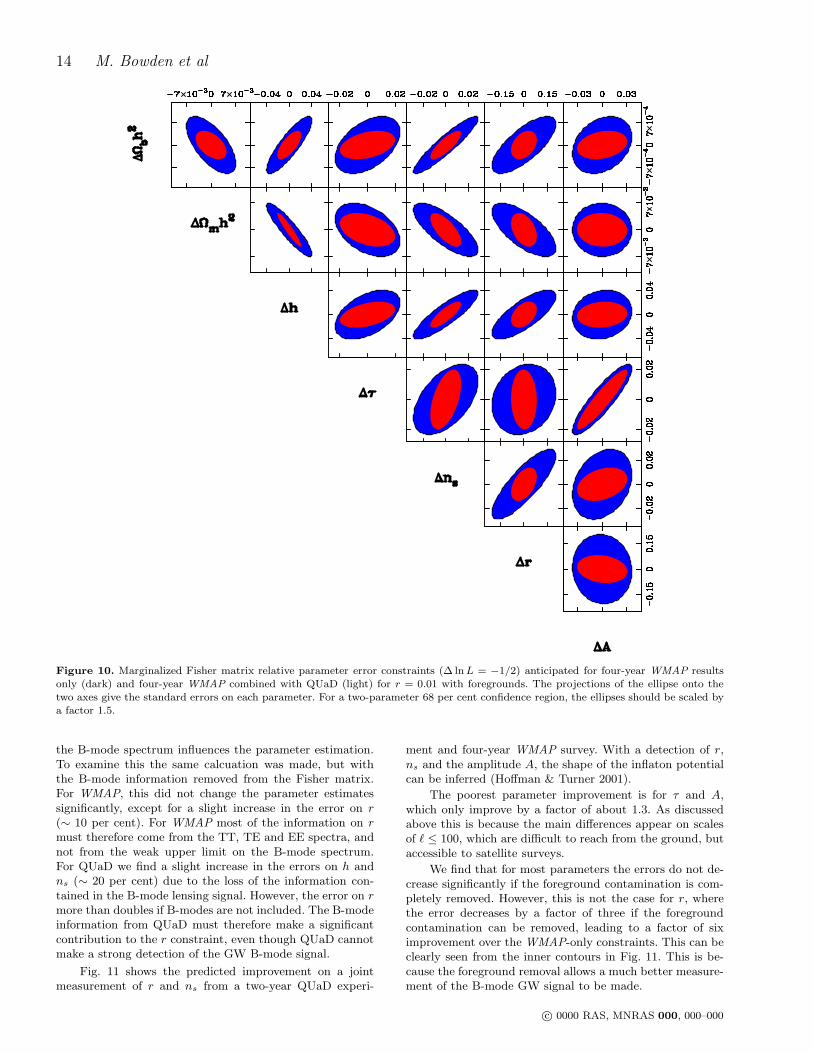
Fig. 10 shows the relative error ellipses (defined by the∆ lnL = −1/2 contour) expected from a 4-year WMAP

experiment (darker ellipses) and from a combined 2-yearground-based QUaD and 4-year WMAP experiment (lighterellipses) for our fiducial 7-parameter model, marginalizingover the other parameters. The projection of this contourgives the marginalized one-parameter, 1 − σ error for eachparameter. For a two-parameter 68 per cent confidence re-gion, the ellispes should be scaled by a factor 1.5. We assumethat the TE-cross spectrum can be estimated in the overlapregion. Here we see that a significant improvement of arounda factor 2 is made on most of the parameter set by adding ina ground-based polarization survey, despite the significantdifference in survey size. For most parameters, this comesfrom the high-multipole information in the EE-spectra, but

c© 0000 RAS, MNRAS 000, 000–000

Optimization of a ground-based CMB polarization experiment 13

Figure 8. The derivative of the CMB polarization power spectra with the parameters ΩBh2, Ωmh2, h, and ns. The models are generatedby CMBfast, with fiducial parameters given in the text.

Figure 9. The derivative of the CMB polarization power spectra with the parameters τ , A and r. The models are generated by CMBfast,with fiducial parameters given in the text. Note that the plot is now logarithmic in order that the low ℓ degeneracy breaking between τand A can be observed in the polarization power spectra.

there is also important information in the BB-spectra, inparticular for r, h and ns.

The 1-σ marginalized parameter uncertainties forWMAP and QUaD + WMAP are shown in Table 5. Byincluding QUaD the precision with which the parameterscan be measured is improved by around a factor of two in

most cases. This increase in accuracy arises from the ex-tra information in the EE-spectra from modes ℓ ≥ 100, andfrom the strong BB-spectral dependence on small scales forns and h. Again, for a temperature survey alone Fig. 8 and9 indicate there is no useful information at high-multipoles.

It is interesting to look at how the information from

c© 0000 RAS, MNRAS 000, 000–000

14 M. Bowden et al

Figure 10. Marginalized Fisher matrix relative parameter error constraints (∆ ln L = −1/2) anticipated for four-year WMAP resultsonly (dark) and four-year WMAP combined with QUaD (light) for r = 0.01 with foregrounds. The projections of the ellipse onto thetwo axes give the standard errors on each parameter. For a two-parameter 68 per cent confidence region, the ellipses should be scaled bya factor 1.5.

the B-mode spectrum influences the parameter estimation.To examine this the same calcuation was made, but withthe B-mode information removed from the Fisher matrix.For WMAP, this did not change the parameter estimatessignificantly, except for a slight increase in the error on r(∼ 10 per cent). For WMAP most of the information on rmust therefore come from the TT, TE and EE spectra, andnot from the weak upper limit on the B-mode spectrum.For QUaD we find a slight increase in the errors on h andns (∼ 20 per cent) due to the loss of the information con-tained in the B-mode lensing signal. However, the error on rmore than doubles if B-modes are not included. The B-modeinformation from QUaD must therefore make a significantcontribution to the r constraint, even though QUaD cannotmake a strong detection of the GW B-mode signal.

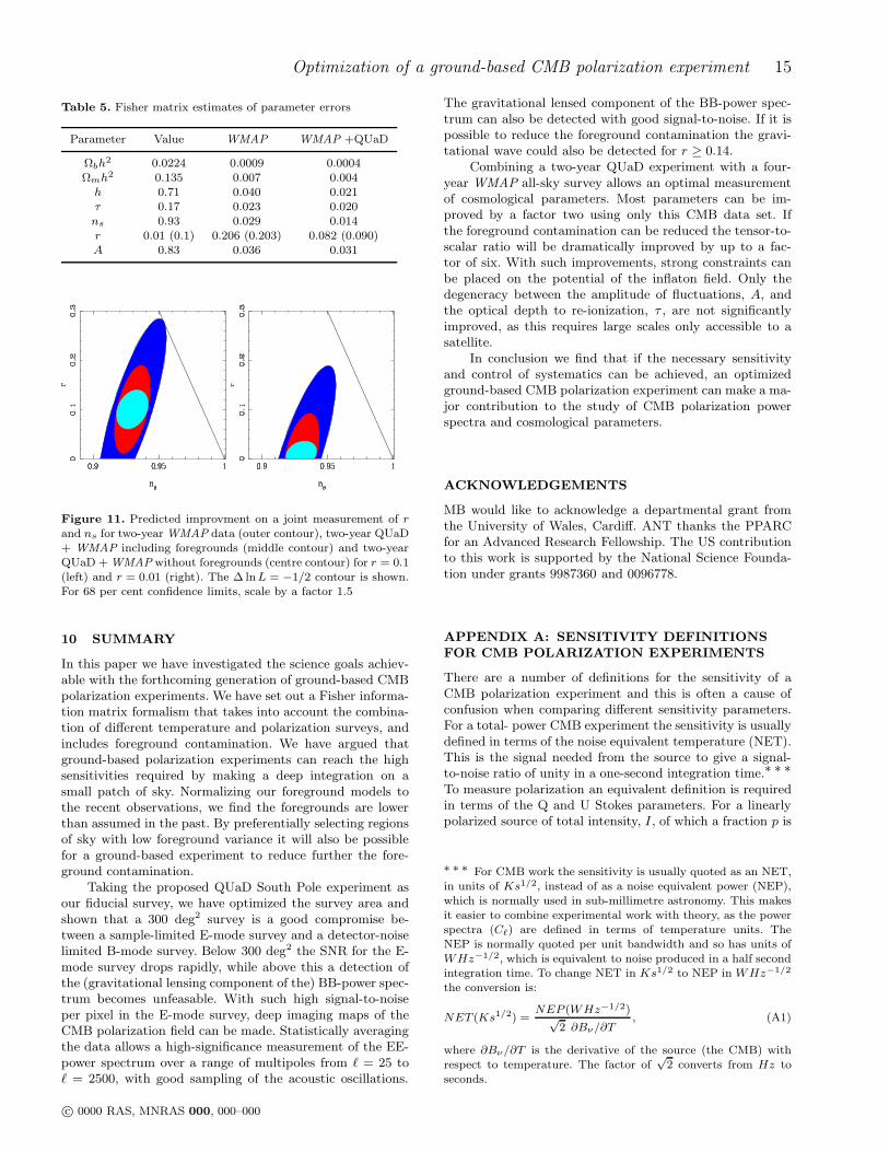
Fig. 11 shows the predicted improvement on a jointmeasurement of r and ns from a two-year QUaD experi-

ment and four-year WMAP survey. With a detection of r,ns and the amplitude A, the shape of the inflaton potentialcan be inferred (Hoffman & Turner 2001).

The poorest parameter improvement is for τ and A,which only improve by a factor of about 1.3. As discussedabove this is because the main differences appear on scalesof ℓ ≤ 100, which are difficult to reach from the ground, butaccessible to satellite surveys.

We find that for most parameters the errors do not de-crease significantly if the foreground contamination is com-pletely removed. However, this is not the case for r, wherethe error decreases by a factor of three if the foregroundcontamination can be removed, leading to a factor of siximprovement over the WMAP-only constraints. This can beclearly seen from the inner contours in Fig. 11. This is be-cause the foreground removal allows a much better measure-ment of the B-mode GW signal to be made.

c© 0000 RAS, MNRAS 000, 000–000

Optimization of a ground-based CMB polarization experiment 15

Table 5. Fisher matrix estimates of parameter errors

Parameter Value WMAP WMAP +QUaD

Ωbh2 0.0224 0.0009 0.0004

Ωmh2 0.135 0.007 0.004h 0.71 0.040 0.021τ 0.17 0.023 0.020ns 0.93 0.029 0.014r 0.01 (0.1) 0.206 (0.203) 0.082 (0.090)A 0.83 0.036 0.031

Figure 11. Predicted improvment on a joint measurement of rand ns for two-year WMAP data (outer contour), two-year QUaD+ WMAP including foregrounds (middle contour) and two-yearQUaD + WMAP without foregrounds (centre contour) for r = 0.1(left) and r = 0.01 (right). The ∆ lnL = −1/2 contour is shown.For 68 per cent confidence limits, scale by a factor 1.5

10 SUMMARY

In this paper we have investigated the science goals achiev-able with the forthcoming generation of ground-based CMBpolarization experiments. We have set out a Fisher informa-tion matrix formalism that takes into account the combina-tion of different temperature and polarization surveys, andincludes foreground contamination. We have argued thatground-based polarization experiments can reach the highsensitivities required by making a deep integration on asmall patch of sky. Normalizing our foreground models tothe recent observations, we find the foregrounds are lowerthan assumed in the past. By preferentially selecting regionsof sky with low foreground variance it will also be possiblefor a ground-based experiment to reduce further the fore-ground contamination.

Taking the proposed QUaD South Pole experiment asour fiducial survey, we have optimized the survey area andshown that a 300 deg2 survey is a good compromise be-tween a sample-limited E-mode survey and a detector-noiselimited B-mode survey. Below 300 deg2 the SNR for the E-mode survey drops rapidly, while above this a detection ofthe (gravitational lensing component of the) BB-power spec-trum becomes unfeasable. With such high signal-to-noiseper pixel in the E-mode survey, deep imaging maps of theCMB polarization field can be made. Statistically averagingthe data allows a high-significance measurement of the EE-power spectrum over a range of multipoles from ℓ = 25 toℓ = 2500, with good sampling of the acoustic oscillations.

The gravitational lensed component of the BB-power spec-trum can also be detected with good signal-to-noise. If it ispossible to reduce the foreground contamination the gravi-tational wave could also be detected for r ≥ 0.14.

Combining a two-year QUaD experiment with a four-year WMAP all-sky survey allows an optimal measurementof cosmological parameters. Most parameters can be im-proved by a factor two using only this CMB data set. Ifthe foreground contamination can be reduced the tensor-to-scalar ratio will be dramatically improved by up to a fac-tor of six. With such improvements, strong constraints canbe placed on the potential of the inflaton field. Only thedegeneracy between the amplitude of fluctuations, A, andthe optical depth to re-ionization, τ , are not significantlyimproved, as this requires large scales only accessible to asatellite.

In conclusion we find that if the necessary sensitivityand control of systematics can be achieved, an optimizedground-based CMB polarization experiment can make a ma-jor contribution to the study of CMB polarization powerspectra and cosmological parameters.

ACKNOWLEDGEMENTS

MB would like to acknowledge a departmental grant fromthe University of Wales, Cardiff. ANT thanks the PPARCfor an Advanced Research Fellowship. The US contributionto this work is supported by the National Science Founda-tion under grants 9987360 and 0096778.

APPENDIX A: SENSITIVITY DEFINITIONS

FOR CMB POLARIZATION EXPERIMENTS

There are a number of definitions for the sensitivity of aCMB polarization experiment and this is often a cause ofconfusion when comparing different sensitivity parameters.For a total- power CMB experiment the sensitivity is usuallydefined in terms of the noise equivalent temperature (NET).This is the signal needed from the source to give a signal-to-noise ratio of unity in a one-second integration time.∗ ∗ ∗To measure polarization an equivalent definition is requiredin terms of the Q and U Stokes parameters. For a linearlypolarized source of total intensity, I , of which a fraction p is

∗ ∗ ∗ For CMB work the sensitivity is usually quoted as an NET,in units of Ks1/2, instead of as a noise equivalent power (NEP),which is normally used in sub-millimetre astronomy. This makesit easier to combine experimental work with theory, as the powerspectra (Cℓ) are defined in terms of temperature units. TheNEP is normally quoted per unit bandwidth and so has units ofWHz−1/2, which is equivalent to noise produced in a half secondintegration time. To change NET in Ks1/2 to NEP in WHz−1/2

the conversion is:

NET (Ks1/2) =NEP (WHz−1/2)√

2 ∂Bν/∂T, (A1)

where ∂Bν/∂T is the derivative of the source (the CMB) withrespect to temperature. The factor of

√2 converts from Hz to

seconds.

c© 0000 RAS, MNRAS 000, 000–000

16 M. Bowden et al

polarized at an angle χ to the reference direction, the Stokesparameters can be defined as:

Q = pI cos(2χ),

U = pI sin(2χ). (A2)

If we orientate the axis of the reference system so that itis aligned with the polarization angle of the source (χ = 0)then we have U = 0 and Q = pI so that Q gives the totalpolarized intensity. We can then define the polarization sen-sitivity, NEQ, as the polarized signal from the source neededto give a signal-to-noise ratio of unity in a one-second inte-gration time for a source with a polarization angle alignedwith the reference direction of the measurement.

For QUaD, the polarized measurements will be madewith pairs of polarization-sensitive bolometers (PSBs). Thetwo bolometers in a PSB pair are sensitive to orthogonalpolarization states of the incoming radiation. The intensitymeasured by the co-polar (x) and cross-polar (y) device isgiven by (Jones et al. 2003):

Ix =1

2(I + Q),

Iy =1

2(I − Q), (A3)

in a reference system aligned with the polarization angle ofthe source. The total intensity is found by adding the twobolometer outputs and the Q Stokes parameter is found bydifferencing the outputs.

For a bolometer, the noise equivalent power due to pho-ton noise (NEP) is given by (Lamarre 1986):

NEP 2 = 2hνP +2P 2

m∆ν(A4)

where is m is the number of polarization states detected (mis either 1 or 2). For a single PSB, m = 1, as only a singlepolarization state is detected. P is the power in a band ofwidth ∆ν:

Pν = ηεAΩBν∆ν, (A5)

where AΩ is the throughput of the system, ε is the emis-sivity of the source and Bν is the intensity of the radiationthat would be emitted from a perfect black body. η is theefficiency of the detector. We assume that a PSB will absorbhalf of the incident unpolarized radiation, giving η = 1/2.The NET due to photon noise in each PSB from the unpo-larized background radiation is therefore:

NETs =(2hνP + 2P 2/∆ν)1/2

η ∂Bν/∂T, (A6)

where the factor of η is needed to convert from the noise atthe detector to the signal required at the source, as only halfof the total unpolarized radiation will be absorbed. ∂Bν/∂Tis the derivative of the source intensity with respect to tem-perature and converts from an NEP to an NET. Equation(A6) gives the NET for a measurement of the temperature

of the CMB with a single PSB.In order to measure the polarization we require a pair

of PSBs. The temperature sensitivity can be obtained byaveraging the two outputs so that:

NETpair = NETs/√

2. (A7)

NETpair is exactly the NET that would be obtained if a sin-gle normal (not polarization sensitive) bolometer had been

used. For a measurement of Q, the two outputs are differ-enced so that:

NEQ =

√2

2NETs =

NETs√2

. (A8)

An important point to note is the extra factor of 2 in the de-nominator. This is because we are now measuring the signalfrom a polarized source, so the extra factor of η which wasneeded to measure the temperature of the source in equa-tion A6 is no-longer required. All of the polarized radiationis absorbed by a single PSB if it is correctly aligned withthe polarization angle of the source.

When defining the sensitivity of a PSB it is thereforeimportant to state whether a sensitivity is an NET for asingle detector, an NET for a pair of detectors, or an NEQfor a pair of detectors. The expression for the pixel noisegiven in Section 3 will depend on the sensitivity definitionused:

σ2 =NET 2Θ2

tobsNPSBθ2. (A9)

If the NET is for a single PSB (as in Table 2 ), NPSB is thetotal number of PSBs. If the sensitivity is given as an NEQfor a PSB pair, NPSB is the number of pairs.

REFERENCES

Baccigalupi C., Perrotta F., De Zotti G., Smoot G.F., BuriganaC., Maino D., Bedini L., Salerno E., 2003, MNRAS, submit-ted, (astro-ph/0209591)

Bennett C. L. et al., 2003, ApJ, accepted, (astro-ph/0302208)

Benoit A. et al., 2003, A&A, 339, L19Bond J. R., Efstathiou G., Tegmark M., 1997, MNRAS, 291, L33-

L41Bunn E. F., 2002, Phys.Rev.D, 65, 043003Church S. E., 2003, The Cosmic Microwave Background and its

Polarization, New Astron. Rev., ed. Hanany S., Olive K. A.Efstathiou G., Bond J. R., 1999, MNRAS, 304, 75Finkbeiner D. P., Davis M., Schlegel D. J., 1999, ApJ, 524, 867Giardino G., Banday A. J., Grski K. M., Bennett K., Jonas J. L.,

Tauber J. 2002, A&A, 387, 82

Guzik J., Seljak U., Zaldarriaga M., 2000, Phys.Rev.D, 64, 043517Halverson L., Lay O., 1998, BAAS, 30, 908Hobson M. P., Jones A. W., Lasenby A. N., Bouchet F. R. 1998,

MNRAS, 300, 1, 29Hobson M. P., Magueijo J., 1996, MNRAS, 283, 4, 1133Hoffman M. B., Turner M. S., 2001, Phys.Rev.D, 64, 2, 023506Hu W., 2001, Phys.Rev.D, 65, 023003Hu W., White M., New Astron., 2, 4, 323

Jaffe A. H., Kamionkowski M., Wang L., 2000, Phys.Rev.D, 61,083501

Jones W. C., Bhatia R., Bock J. J., Lange A. E., 2003, ed Phillips,T. G., Zmuidzinas, J., Proc. of the SPIE, 4855, 227

Kamionkowski M., Kosowsky A., Stebbins A., 1997, Phys.Rev.D,55, 12, 7368

Kaplinghat M., Knox K., Song Y., 2003, preprint (astro-ph/0303344)

Keating B., Timbie P., Polnarev A., Steinberger J., 1998, ApJ,495, 580

Kesden M., Cooray A., Kamionkowski M., 2002, Phys.Rev.Lett,89, 1, 011304

Knox L., Song S., 2002, Phys.Rev.Lett, 89, 1, 011303Kogut A. et al, 2003, ApJ, accepted (astro-ph/0302213)Kovac J., Leitch E. M., Pryke C., Carlstrom J. E, Halverson N.

W., Holzapfel W. L., 2002, Nat, 420, 772

c© 0000 RAS, MNRAS 000, 000–000

Optimization of a ground-based CMB polarization experiment 17

Lamarre J., 1986, Applied Opt., 25, 870

Leach S. M., Liddle A. R., 2003, preprint (astro-ph/0306305)Lewis A., Challinor A., Turok N., 2002, Phys.Rev.D, 65, 2, 023505Maino D., et al., 2002, MNRAS, 334, 1, 53Montroy T. et al., 2003, preprint (astro-ph/0305593)Seljak U., Zaldarriaga M., 1996, ApJ, 469, 473Spergel D. N., et al., 2003, ApJ, accepted, (astro-ph/0302209)Tegmark M., Eisenstein D. J., Hu W., Oliveira-Costa A., 2000,

ApJ, 530, 133Tegmark M., Taylor A. N., Heavens A. F., 1997, ApJ, 480, 22Turner, M., S., 1996, Phys.Rev.D, 53, 12, 6822Verde L., et al., 2003, ApJ, accepted, (astro-ph/0302218)Zaldarriaga, M., 2003, American Astronomical Society Meeting,

202, 5601ZZaldarriaga, M., Seljak, U., 1997, Phys.Rev.D, 55, 1830Zaldarriaga, M., Spergel, D. N., Seljak, U., 1997, ApJ, 488, 1

c© 0000 RAS, MNRAS 000, 000–000