MoleculeNet: A Benchmark for Molecular Machine Learning

MoleculeNet: A Benchmark for Molecular

Machine Learning

Zhenqin Wu,†,‖ Bharath Ramsundar,‡,‖ Evan N. Feinberg,¶,⊥ Joseph Gomes,†,⊥

Caleb Geniesse,¶ Aneesh S. Pappu,‡ Karl Leswing,§ and Vijay Pande∗,†

†Department of Chemistry, Stanford University

‡Department of Computer Science, Stanford University

¶Program in Biophysics, Stanford School of Medicine

§Schrodinger Inc.

‖Joint First Authorship

⊥Joint Second Authorship

E-mail: [email protected]

Abstract

Molecular machine learning has been maturing rapidly over the last few years.

Improved methods and the presence of larger datasets have enabled machine learning

algorithms to make increasingly accurate predictions about molecular properties. How-

ever, algorithmic progress has been limited due to the lack of a standard benchmark to

compare the efficacy of proposed methods; most new algorithms are benchmarked on

different datasets making it challenging to gauge the quality of proposed methods. This

work introduces MoleculeNet, a large scale benchmark for molecular machine learn-

ing. MoleculeNet curates multiple public datasets, establishes metrics for evaluation,

and offers high quality open-source implementations of multiple previously proposed

molecular featurization and learning algorithms (released as part of the DeepChem

1

arX

iv:1

703.

0056

4v3

[cs

.LG

] 2

6 O

ct 2

018

[email protected]

open source library). MoleculeNet benchmarks demonstrate that learnable represen-

tations are powerful tools for molecular machine learning and broadly offer the best

performance. However, this result comes with caveats. Learnable representations still

struggle to deal with complex tasks under data scarcity and highly imbalanced classi-

fication. For quantum mechanical and biophysical datasets, the use of physics-aware

featurizations can be more important than choice of particular learning algorithm.

Introduction

Overlap between chemistry and statistical learning has had a long history. The field of chem-

informatics has been utilizing machine learning methods in chemical modeling(e.g. quanti-

tative structure activity relationships, QSAR) for decades.1–6 In the recent 10 years, with

the advent of sophisticated deep learning methods,7,8 machine learning has gathered increas-

ing amounts of attention from the scientific community. Data-driven analysis has become

a routine step in many chemical and biological applications, including virtual screening,9–12

chemical property prediction,13–16 and quantum chemistry calculations.17–20

In many such applications, machine learning has shown strong potential to compete with

or even outperform conventional ab-initio computations.16,18 It follows that introduction

of novel machine learning methods has the potential to reshape research on properties of

molecules. However, this potential has been limited by the lack of a standard evaluation

platform for proposed machine learning algorithms. Algorithmic papers often benchmark

proposed methods on disjoint dataset collections, making it a challenge to gauge whether a

proposed technique does in fact improve performance.

Data for molecule-based machine learning tasks are highly heterogeneous and expensive

to gather. Obtaining precise and accurate results for chemical properties typically requires

specialized instruments as well as expert supervision (contrast with computer speech and

vision, where lightly trained workers can annotate data suitable for machine learning sys-

tems). As a result, molecular datasets are usually much smaller than those available for

2

other machine learning tasks. Furthermore, the breadth of chemical research means our

interests with respect to a molecule may range from quantum characteristics to measured

impacts on the human body. Molecular machine learning methods have to be capable of

learning to predict this very broad range of properties. Complicating this challenge, input

molecules can have arbitrary size and components, highly variable connectivity and many

three dimensional conformers (three dimensional molecular shapes). To transform molecules

into a form suitable for conventional machine learning algorithms (that usually accept fixed

length input), we have to extract useful and related information from a molecule into a fixed

dimensional representation (a process called featurization).21–23

To put it simply, building machine learning models on molecules requires overcoming

several key issues: limited amounts of data, wide ranges of outputs to predict, large hetero-

geneity in input molecular structures and appropriate learning algorithms. Therefore, this

work aims to facilitate the development of molecular machine learning methods by curating

a number of dataset collections, creating a suite of software that implements many known

featurizations of molecules, and providing high quality implementations of many previously

proposed algorithms. Following the footsteps of WordNet24 and ImageNet,25 we call our

suite MoleculeNet, a benchmark collection for molecular machine learning.

In machine learning, a benchmark serves as more than a simple collection of data and

methods. The introduction of the ImageNet benchmark in 2009 has triggered a series of

breakthroughs in computer vision, and in particular has facilitated the rapid development of

deep convolutional networks. The ILSVRC, an annual contest held by the ImageNet team,26

draws considerable attention from the community, and greatly stimulates collaborations and

competitions across the field. The contest has given rise to a series of prominent machine

learning models such as AlexNet,27 GoogLeNet,28 ResNet29 which have had broad impact on

the academic and industrial computer science communities. We hope that MoleculeNet will

trigger similar breakthroughs by serving as a platform for the wider community to develop

and improve models for learning molecular properties.

3

In particular, MoleculeNet contains data on the properties of over 700,000 compounds.

All datasets have been curated and integrated into the open source DeepChem package.30

Users of DeepChem can easily load all MoleculeNet benchmark data through provided library

calls. MoleculeNet also contributes high quality implementations of well known (bio)chemical

featurization methods. To facilitate comparison and development of new methods, we also

provide high quality implementations of several previously proposed machine learning meth-

ods. Our implementations are integrated with DeepChem, and depend on Scikit-Learn31

and Tensorflow32 underneath the hood. Finally, evaluation of machine learning algorithms

requires defined methods to split datasets into training/validation/test collections. Random

splitting, common in machine learning, is often not correct for chemical data.33 MoleculeNet

contributes a library of splitting mechanisms to DeepChem and evaluates all algorithms with

multiple choices of data split. MoleculeNet provide a series of benchmark results of imple-

mented machine learning algorithms using various featurizations and splits upon our dataset

collections. These results are provided within this paper, and will be maintained online in

an ongoing fashion as part of DeepChem.

The related work section will review prior work in the chemistry community on gather-

ing curated datasets and discuss how MoleculeNet differs from these previous efforts. The

methods section reviews the dataset collections, metrics, featurization methods, and ma-

chine learning models included as part of MoleculeNet. The results section will analyze the

benchmarking results to draw conclusions about the algorithms and datasets considered.

Related Work

MoleculeNet draws upon a broader movement within the chemical community to gather large

sources of curated data. PubChem34 and PubChem BioAssasy35 gather together thousands

of bioassay results, along with millions of unique molecules tested within these assays. The

ChEMBL database offers a similar service, with millions of bioactivity outcomes across thou-

4

sands of protein targets. Both PubChem and ChEMBL are human researcher oriented, with

web portals that facilitate browsing of the available targets and compounds. ChemSpider is

a repository of nearly 60 million chemical structures, with web based search capabilities for

users. The Crystallography Open Database36 and Cambridge Structural Database37 offer

large repositories of organic and inorganic compounds. The protein data bank38 offers a

repository of experimentally resolved three dimensional protein structures. This listing is by

no means comprehensive; the methods section will discuss a number of smaller data sources

in greater detail.

These past efforts have been critical in enabling the growth of computational chemistry.

However, these previous databases are not machine-learning focused. In particular, these

collections don’t define metrics which measure the effectiveness of algorithmic methods in

understanding the data contained. Furthermore, there is no prescribed separation of the data

into training/validation/test sets (critical for machine learning development). Without spec-

ified metrics or splits, the choice is left to individual researchers, and there are indeed many

chemical machine learning papers which use subsets of these data stores for machine learning

evaluation. Unfortunately, the choice of metric and subset varies widely between groups, so

two methods papers using PubChem data may be entirely incomparable. MoleculeNet aims

to bridge this gap by providing benchmark results for a reasonable range of metrics, splits,

and subsets of these (and other) data collections.

It’s important to note that there have been some efforts to create benchmarking datasets

for machine learning in chemistry. The Quantum Machine group39 and previous work on

multitask learning10 both introduce benchmarking collections which have been used in multi-

ple papers. MoleculeNet incorporates data from both these efforts and significantly expands

upon them.

5

Methods

MoleculeNet is based on the open source package DeepChem.30 Figure 1 shows an annotated

DeepChem benchmark script. Note how different choices for data splitting, featurization,

and model are available. DeepChem also directly provides molnet sub-module to support

benchmarking. The single line below runs benchmarking on the specified dataset, model and

featurizer. User defined models capable of handling DeepChem datasets are also supported.

deepchem.molnet.run benchmark(datasets, model, split, featurizer)

In this section, we will further elaborate the benchmarking system, introducing available

datasets as well as implemented splitting, metrics, featurization, and learning methods.

Figure 1: Example code for benchmark evaluation with DeepChem, multiple methods areprovided for data splitting, featurization and learning.

Datasets

MoleculeNet is built upon multiple public databases. The full collection currently includes

over 700,000 compounds tested on a range of different properties. These properties can

be subdivided into four categories: quantum mechanics, physical chemistry, biophysics and

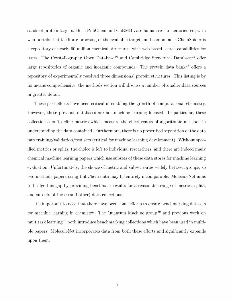
physiology. As illustrated in Figure 2, separate datasets in the MoleculeNet collection cover

6

various levels of molecular properties, ranging from molecular-level properties to macro-

scopic influences on human body. For each dataset, we propose a metric and a splitting

pattern(introduced in the following texts) that best fit the properties of the dataset. Perfor-

mances on the recommended metric and split are reported in the results section.

In most datasets, SMILES strings40 are used to represent input molecules, 3D coordinates

are also included in part of the collection as molecular features, which enabled different

methods to be applied. Properties, or output labels, are either 0/1 for classification tasks,

or floating point numbers for regression tasks. At the time of writing, MoleculeNet contains

17 datasets prepared and benchmarked, but we anticipate adding further datasets in an on-

going fashion. We also highly welcome contributions from other public data collections. For

more detailed dataset structure requirements and instructions on curating datasets, please

refer to the tutorial on DeepChem webpage.

Table 1 lists details of datasets in the collection, including tasks, compounds and their

features, recommended splits and metrics. Contents of each dataset will be elaborated in

this subsection.

Figure 2: Tasks in different datasets focus on different levels of properties of molecules.

QM7/QM7b

The QM7/QM7b datasets are subsets of the GDB-13 database,41 a database of nearly 1

billion stable and synthetically accessible organic molecules, containing up to seven “heavy”

7

Table 1: Dataset Details: number of compounds and tasks, recommended splits and metrics

Category Dataset Data Type # Tasks Task Type # Compounds Rec - Split Rec - Metric

Quantum Mechanics

QM7 SMILES, 3D coordinates 1 Regression 7160 Stratified MAEQM7b 3D coordinates 14 Regression 7210 Random MAEQM8 SMILES, 3D coordinates 12 Regression 21786 Random MAEQM9 SMILES, 3D coordinates 12 Regression 133885 Random MAE

Physical ChemistryESOL SMILES 1 Regression 1128 Random RMSE

FreeSolv SMILES 1 Regression 642 Random RMSELipophilicity SMILES 1 Regression 4200 Random RMSE

Biophysics

PCBA SMILES 128 Classification 437929 Random PRC-AUCMUV SMILES 17 Classification 93087 Random PRC-AUCHIV SMILES 1 Classification 41127 Scaffold ROC-AUC

PDBbind SMILES, 3D coordinates 1 Regression 11908 Time RMSEBACE SMILES 1 Classification 1513 Scaffold ROC-AUC

Physiology

BBBP SMILES 1 Classification 2039 Scaffold ROC-AUCTox21 SMILES 12 Classification 7831 Random ROC-AUC

ToxCast SMILES 617 Classification 8575 Random ROC-AUCSIDER SMILES 27 Classification 1427 Random ROC-AUCClinTox SMILES 2 Classification 1478 Random ROC-AUC

atoms (C, N, O, S). The 3D Cartesian coordinates of the most stable conformation and elec-

tronic properties (atomization energy, HOMO/LUMO eigenvalues, etc.) of each molecule

were determined using ab-initio density functional theory (PBE0/tier2 basis set).17,18 Learn-

ing methods benchmarked on QM7/QM7b are responsible for predicting these electronic

properties given stable conformational coordinates. For the purpose of more stable perfor-

mances as well as better comparison, we recommend stratified splitting(introduced in the

next subsection) for QM7.

QM8

The QM8 dataset comes from a recent study on modeling quantum mechanical calculations

of electronic spectra and excited state energy of small molecules.42 Multiple methods, in-

cluding time-dependent density functional theories (TDDFT) and second-order approximate

coupled-cluster (CC2), are applied to a collection of molecules that include up to eight heavy

atoms (also a subset of the GDB-17 database43). In total, four excited state properties are

calculated by three different methods on 22 thousand samples.

QM9

QM9 is a comprehensive dataset that provides geometric, energetic, electronic and ther-

modynamic properties for a subset of GDB-17 database,43 comprising 134 thousand stable

organic molecules with up to nine heavy atoms.44 All molecules are modeled using density

8

functional theory (B3LYP/6-31G(2df,p) based DFT). In our benchmark, geometric prop-

erties (atomic coordinates) are integrated into features, which are then applied to predict

other properties.

The datasets introduced above (QM7, QM7b, QM8, QM9) were curated as part of the

Quantum-Machine effort,39 which has processed a number of datasets to measure the efficacy

of machine-learning methods for quantum chemistry.

ESOL

ESOL is a small dataset consisting of water solubility data for 1128 compounds.13 The dataset

has been used to train models that estimate solubility directly from chemical structures (as

encoded in SMILES strings).22 Note that these structures don’t include 3D coordinates, since

solubility is a property of a molecule and not of its particular conformers.

FreeSolv

The Free Solvation Database (FreeSolv) provides experimental and calculated hydration free

energy of small molecules in water.16 A subset of the compounds in the dataset are also

used in the SAMPL blind prediction challenge.15 The calculated values are derived from

alchemical free energy calculations using molecular dynamics simulations. We include the

experimental values in the benchmark collection, and use calculated values for comparison.

Lipophilicity

Lipophilicity is an important feature of drug molecules that affects both membrane perme-

ability and solubility. This dataset, curated from ChEMBL database,45 provides experimen-

tal results of octanol/water distribution coefficient (logD at pH 7.4) of 4200 compounds.

9

PCBA

PubChem BioAssay (PCBA) is a database consisting of biological activities of small molecules

generated by high-throughput screening.35 We use a subset of PCBA, containing 128 bioas-

says measured over 400 thousand compounds, used by previous work to benchmark machine

learning methods.10

MUV

The Maximum Unbiased Validation (MUV) group is another benchmark dataset selected

from PubChem BioAssay by applying a refined nearest neighbor analysis.46 The MUV

dataset contains 17 challenging tasks for around 90 thousand compounds and is specifically

designed for validation of virtual screening techniques.

HIV

The HIV dataset was introduced by the Drug Therapeutics Program (DTP) AIDS Antiviral

Screen, which tested the ability to inhibit HIV replication for over 40,000 compounds.47

Screening results were evaluated and placed into three categories: confirmed inactive (CI),

confirmed active (CA) and confirmed moderately active (CM). We further combine the lat-

ter two labels, making it a classification task between inactive (CI) and active (CA and

CM). As we are more interested in discover new categories of HIV inhibitors, scaffold split-

ting(introduced in the next subsection) is recommended for this dataset.

PDBbind

PDBbind is a comprehensive database of experimentally measured binding affinities for bio-

molecular complexes.48,49 Unlike other ligand-based biological activity datasets, in which only

the structures of ligands are provided, PDBbind provides detailed 3D Cartesian coordinates

of both ligands and their target proteins derived from experimental (e.g., X-Ray crystal-

lography) measurements. The availability of coordinates of the protein-ligand complexes

10

permits structure-based featurization that is aware of the protein-ligand binding geometry.

We use the “refined” and “core” subsets of the database,50 more carefully processed for data

artifacts, as additional benchmarking targets. Samples in PDBbind dataset are collected

over a relatively long period of time(since 1982), hence a time splitting pattern(introduced

in the next subsection) is recommended to mimic actual development in the field.

BACE

The BACE dataset provides quantitative (IC50) and qualitative (binary label) binding results

for a set of inhibitors of human β-secretase 1 (BACE-1).51 All data are experimental values

reported in scientific literature over the past decade, some with detailed crystal structures

available. We merged a collection of 1522 compounds with their 2D structures and binary

labels in MoleculeNet, built as a classification task. Similarly, regarding a single protein

target, scaffold splitting will be more practically useful.

BBBP

The Blood-brain barrier penetration (BBBP) dataset comes from a recent study52 on the

modeling and prediction of the barrier permeability. As a membrane separating circulating

blood and brain extracellular fluid, the blood-brain barrier blocks most drugs, hormones and

neurotransmitters. Thus penetration of the barrier forms a long-standing issue in develop-

ment of drugs targeting central nervous system. This dataset includes binary labels for over

2000 compounds on their permeability properties. Scaffold splitting is also recommended for

this well-defined target.

Tox21

The “Toxicology in the 21st Century” (Tox21) initiative created a public database mea-

suring toxicity of compounds, which has been used in the 2014 Tox21 Data Challenge.53

This dataset contains qualitative toxicity measurements for 8014 compounds on 12 different

11

targets, including nuclear receptors and stress response pathways.

ToxCast

ToxCast is another data collection (from the same initiative as Tox21) providing toxicology

data for a large library of compounds based on in vitro high-throughput screening.54 The

processed collection in MoleculeNet includes qualitative results of over 600 experiments on

8615 compounds.

SIDER

The Side Effect Resource (SIDER) is a database of marketed drugs and adverse drug reac-

tions (ADR).55 The version of the SIDER dataset in DeepChem56 has grouped drug side-

effects into 27 system organ classes following MedDRA classifications57 measured for 1427

approved drugs (following previous usage56).

ClinTox

The ClinTox dataset, introduced as part of this work, compares drugs approved by the FDA

and drugs that have failed clinical trials for toxicity reasons.58,59 The dataset includes two

classification tasks for 1491 drug compounds with known chemical structures: (1) clinical

trial toxicity (or absence of toxicity) and (2) FDA approval status. List of FDA-approved

drugs are compiled from the SWEETLEAD database,60 and list of drugs that failed clinical

trials for toxicity reasons are compiled from the Aggregate Analysis of ClinicalTrials.gov

(AACT) database.61

Dataset splitting

Typical machine learning methods require datasets to be split into training/validation/test

subsets (or alternatively into K-folds) for benchmarking. All MoleculeNet datasets are split

into training, validation and test, following a 80/10/10 ratio. Training sets were used to

12

Figure 3: Representation of Data Splits in MoleculeNet.

train models, while validation sets were used for tuning hyperparameters, and test sets were

used for evaluation of models.

As mentioned previously, random splitting of molecular data isn’t always best for eval-

uating machine learning methods. Consequently, MoleculeNet implements multiple differ-

ent splittings for each dataset. Random splitting randomly splits samples into the train-

ing/validation/test subsets. Scaffold splitting splits the samples based on their two-dimensional

structural frameworks,62 as implemented in RDKit.63 Since scaffold splitting attempts to sep-

arate structurally different molecules into different subsets, it offers a greater challenge for

learning algorithms than the random split.

In addition, a stratified random sampling method is implemented on the QM7 dataset

to reproduce the results from the original work.18 This method sorts datapoints in order of

increasing label value (note this is only defined for real-valued output). This sorted list is then

split into training/validation/test by ensuring that each set contains the full range of provided

labels. Time splitting is also adopted for dataset that includes time information(PDBbind).

13

Under this splitting method, model will be trained on older data and tested on newer data,

mimicking real world development condition.

MoleculeNet contributes the code for these splitting methods into DeepChem. Users of

the library can use these splits on new datasets with short library calls.

Metrics

MoleculeNet contains both regression datasets (QM7, QM7b, QM8, QM9, ESOL, Free-

Solv, Lipophilicity and PDBbind) and classification datasets (PCBA, MUV, HIV, BACE,

BBBP, Tox21, ToxCast and SIDER). Consequently, different performance metrics need to

be measured for each. Following suggestions from the community,64 regression datasets are

evaluated by mean absolute error (MAE) and root-mean-square error (RMSE), classification

datasets are evaluated by area under curve (AUC) of the receiver operating characteristic

(ROC) curve65 and the precision recall curve (PRC).66 For datasets containing more than

one task, we report the mean metric values over all tasks.

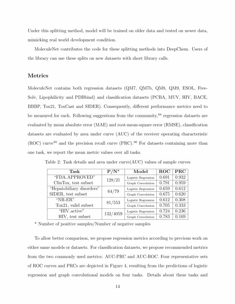
Table 2: Task details and area under curve(AUC) values of sample curves

Task P/N* Model ROC PRC“FDA APPROVED”ClinTox, test subset

128/21Logistic Regression 0.691 0.932Graph Convolution 0.791 0.959

“Hepatobiliary disorders”SIDER, test subset


“NR-ER”Tox21, valid subset


“HIV active”HIV, test subset


* Number of positive samples/Number of negative samples

To allow better comparison, we propose regression metrics according to previous work on

either same models or datasets. For classification datasets, we propose recommended metrics

from the two commonly used metrics: AUC-PRC and AUC-ROC. Four representative sets

of ROC curves and PRCs are depicted in Figure 4, resulting from the predictions of logistic

regression and graph convolutional models on four tasks. Details about these tasks and

14

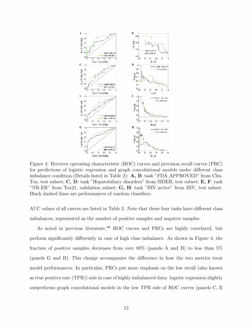
Figure 4: Receiver operating characteristic (ROC) curves and precision recall curves (PRC)for predictions of logistic regression and graph convolutional models under different classimbalance condition.(Details listed in Table 2): A, B: task ”FDA APPROVED” from Clin-Tox, test subset; C, D: task ”Hepatobiliary disorders” from SIDER, test subset; E, F: task”NR-ER” from Tox21, validation subset; G, H: task ”HIV active” from HIV, test subset.Black dashed lines are performances of random classifiers.

AUC values of all curves are listed in Table 2. Note that these four tasks have different class

imbalances, represented as the number of positive samples and negative samples.

As noted in previous literature,66 ROC curves and PRCs are highly correlated, but

perform significantly differently in case of high class imbalance. As shown in Figure 4, the

fraction of positive samples decreases from over 80% (panels A and B) to less than 5%

(panels G and H). This change accompanies the difference in how the two metrics treat

model performances. In particular, PRCs put more emphasis on the low recall (also known

as true positive rate (TPR)) side in case of highly imbalanced data: logistic regression slightly

outperforms graph convolutional models in the low TPR side of ROC curves (panels C, E

15

and G, lower left corner), which creates different margins on the low recall side of PRCs.

ROC curves and PRCs share one same axis, while using false positive rate (FPR) and

precision for the other axis respectively. Recall that FPR and precision are defined as follows:

FPR =False Positive

False Positive + True Negative

Precision =True Positive

False Positive + True Positive

When positive samples form only a small proportion of all samples, false positive predic-

tions exert a much greater influence on precision than FPR, amplifying the difference between

PRC and ROC curves. Virtual screening experiments do have extremely low positive rates,

suggesting that the correct metric to analyze may depend on the experiment at hand. In this

work, we hence propose recommended metrics based on positive rates, PRC-AUC is used for

datasets with positive rates less than 2%, otherwise ROC-AUC is used.

Featurization

A core challenge for molecular machine learning is effectively encoding molecules into fixed-

length strings or vectors. Although SMILES strings are unique representations of molecules,

most molecular machine learning methods require further information to learn sophisticated

electronic or topological features of molecules from limited amounts of data. (Recent work

has demonstrated the ability to learn useful representations from SMILES strings using more

sophisticated methods,67 so it may be feasible to use SMILES strings for further learning

tasks in the near future.) Furthermore, the enormity of chemical space often requires repre-

sentations of molecules specifically suited to the learning task at hand. MoleculeNet contains

implementations of six useful molecular featurization methods.

ECFP

Extended-Connectivity Fingerprints (ECFP) are widely-used molecular characterizations in

chemical informatics.21 During the featurization process, a molecule is decomposed into

16

Figure 5: Diagrams of featurizations in MoleculeNet.

submodules originated from heavy atoms, each assigned with a unique identifier. These

segments and identifiers are extended through bonds to generate larger substructures and

corresponding identifiers.

After hashing all these substructures into a fixed length binary fingerprint, the representa-

tion contains information about topological characteristics of the molecule, which enables it

to be applied to tasks such as similarity searching and activity prediction. The MoleculeNet

implementation uses ECFP4 fingerprints generated by RDKit.63

17

Coulomb Matrix

Ab-initio electronic structure calculations typically require a set of nuclear charges {Z} and

the corresponding Cartesian coordinates {R} as input. The Coulomb Matrix (CM) M,

proposed by Rupp et al.17 and defined below, encodes this information by use of the atomic

self-energies and internuclear Coulomb repulsion operator.

MIJ =

0.5Z2.4

I for I = J

ZIZJ

|RI−RJ |for I 6= J

Here, the off-diagonal elements correspond to the Coulomb repulsion between atoms I

and J, and the diagonal elements correspond to a polynomial fit of atomic self-energy to

nuclear charge. The Coulomb Matrix of a molecule is invariant to translation and rotation

of that molecule, but not with respect to atom index permutation. In the construction of

coulomb matrix, we first use the nuclear charges and distance matrix generated by RDKit63

to acquire the original coulomb matrix, then an optional random atom index sorting and

binary expansion transformation can be applied during training in order to achieve atom

index invariance, as reported by Montavon et al.18

Grid Featurizer

The grid featurizer is a featurization method (introduced in the current work) initially de-

signed for the PDBbind dataset in which structural information of both the ligand and

target protein are considered. Since binding affinity stems largely from the intermolecular

forces between ligands and proteins, in addition to intramolecular interactions, we seek to

incorporate both the chemical interaction within the binding pocket as well as features of

the protein and ligand individually.

The grid featurizer was inspired by the NNscore featurizer68 and SPLIF69 but optimized

18

for speed, robustness, and generalizability. The intermolecular interactions enumerated by

the featurizer include salt bridges and hydrogen bonding between protein and ligand, intra-

ligand circular fingerprints, intra-protein circular fingerprints, and protein-ligand SPLIF fin-

gerprints. A more detailed breakdown can be found in the Appendix.

Symmetry Function

Symmetry function, first introduced by Behler and Parrinello,70 is another common encoding

of atomic coordinates information. It focuses on preserving the rotational and permutation

symmetry of the system. The local environment of an atom in the molecule is expressed as a

series of radial and angular symmetry functions with different distance and angle cutoffs, the

former focusing on distances between atom pairs and the latter focusing on angles formed

within triplets of atoms.

As symmetry function put most emphasis on spatial positions of atoms, it is intrinsically

hard for it to distinguish different atom types(H, C, O). MoleculeNet utilized a slightly

modified version of original symmetry function71 which further separate radial and angular

symmetry terms according to the type of atoms in the pair or triplet. Further details can be

found in the article71 or our implementation.

Graph Convolutions

The graph convolutions featurization support most graph-based models. It computes an

initial feature vector and a neighbor list for each atom. The feature vector summarizes the

atom’s local chemical environment, including atom-type, hybridization type, and valence

structure. Neighbor lists represent connectivity of the whole molecule, which are further

processed in each model to generate graph structures (discussed in further details in following

parts).

19

Weave

Similar to graph convolutions, the weave featurization encodes both local chemical environ-

ment and connectivity of atoms in a molecule. Atomic feature vectors are exactly the same,

while connectivity is represented by more detailed pair features instead of neighbor listing.

The weave featurization calculates a feature vector for each pair of atoms in the molecule,

including bond properties (if directly connected), graph distance and ring info, forming a

feature matrix. The method supports graph-based models that utilize properties of both

nodes (atoms) and edges (bonds).

Models - Conventional Models

MoleculeNet tests the performance of various machine learning models on the datasets dis-

cussed previously. These models could be further categorized into conventional methods and

graph-based methods according to their structures and input types. The following sections

will give brief introductions to benchmarked algorithms. The results section will discuss per-

formance numbers in detail. Here we briefly review conventional methods including logistic

regression, support vector classification, kernel ridge regression, random forests,72 gradient

boosting,73 multitask networks,9,10 bypass networks74 and influence relevance voting.75 The

next section graph-based models will give introductions to graph convolutional models,22

weave models,23 directed acyclic graph models,14 deep tensor neural networks,19 ANI-171

and message passing neural networks.76 As part of this work, all methods are implemented

in the open source DeepChem package.30

Logistic Regression

Logistic regression models (Logreg) apply the logistic function to weighted linear combina-

tions of their input features to obtain model predictions. It is often common to use regular-

ization to encourage learned weights to be sparse.77 Note that logistic regression models are

only defined for classification tasks.

20

Support Vector Classification

Support vector machine (SVM) is one of the most famous and widely-used machine learning

method.78 As in classification task, it defines a decision plane which separates data points

of different class with maximized margin. To further increase performance, we incorporates

regularization and a radial basis function kernel (KernelSVM).

Kernel Ridge Regression

Kernel ridge regression(KRR) is a combination of ridge regression and kernel trick. By

using a nonlinear kernel function(radial basis function), it learns a non-linear function in the

original space that maps features to predicted values.

Random Forests

Random forests (RF) are ensemble prediction methods.72 A random forest consists of many

individual decision trees, each of which is trained on a subsampled version of the original

dataset. The results for individual trees are averaged to provide output predictions for the

full forest. Random forests can be used for both classification and regression tasks. Training

a random forest can be computationally intensive, so benchmarks only include random forest

results for smaller datasets.

Gradient Boosting

Gradient boosting is another ensemble method consisting of individual decision trees.73 In

contrast to random forests, it builds relatively simple trees which are sequentially incorpo-

rated to the ensemble. In each step, a new tree is generated in a greedy manner to minimize

loss function. A sequence of such ”weak” trees are combined together into an additive model.

We utilize the XGBoost implementation of gradient boosting in DeepChem.79

21

Multitask/Singletask Network

In a multitask network,10 input featurizations are processed by fully connected neural net-

work layers. The processed output is shared among all learning tasks in a dataset, and

then fed into separate linear classifiers/regressors for each different task. In the case that

a dataset contains only a single task, multitask networks are just fully connected neural

networks(Singletask Network). Since multitask networks are trained on the joint data avail-

able for various tasks, the parameters of the shared layers are encouraged to produce a joint

representation which can share information between learning tasks. This effect does seem

to have limitations; merging data from uncorrelated tasks has only moderate effect.80 As a

result, MoleculeNet does not attempt to train extremely large multitask networks combining

all data for all datasets.

Bypass Multitask Networks

Multitask modeling relies on the fact that some features have explanatory power that is

shared among multiple tasks. Note that the opposite may well be true; features useful for

one task can be detrimental to other tasks. As a result, vanilla multitask networks can

lack the power to explain unrelated variations in the samples. Bypass networks attempt

to overcome this variation by merging in per-task independent layers that “bypass” shared

layers to directly connect inputs with outputs.74 In other words, bypass multitask networks

consist of ntasks + 1 independent components: one “multitask” layer mapping all inputs to

shared representations, and ntasks “bypass” layers mapping inputs for each specific task to

their labels. As the two groups have separate parameters, bypass networks may have greater

explanatory power than vanilla multitask networks.

Influence Relevance Voting

Influence Relevance Voting (IRV) systems are refined K-nearest neighbor classifiers.75 Using

the hypothesis that compounds with similar substructures have similar functionality, the

22

IRV classifier makes its prediction by combining labels from the top K compounds most

similar to a provided test sample.

The Jaccard-Tanimoto similarity between fingerprints of compounds is used as the simi-

larity measurement:

S( ~A, ~B) =A ∩BA ∪B

Then IRV model calculates a weighted sum of the labels of top K similar compounds to

predict the result, in which weights are the outputs of a one-hidden layer neural network

with similarities and rankings of top K compounds as input. Detailed descriptions of the

model can be found in the original article.75

Models - Graph Based Models

Early attempts to directly use molecular structures instead of selected features has emerged

in 1990s.81,82 While in recent years, models propelled by the very similar idea start to grow

rapidly. These specifically designed methods, namely graph-based models, are naturally

suitable for modeling molecules. By defining atoms as nodes, bonds as edges, molecules can

be modeled as mathematical graphs. As noted in a recent paper,76 this natural similarity

has inspired a number of models to utilize the graph structure of molecules to gain higher

performances. In general, graph-based models apply adaptive functions to nodes and edges,

allowing for a learnable featurization process. MoleculeNet provides implementations of mul-

tiple graph-based models which use different variants of molecular graphs. We describe these

methods in the following sections. Figure 6 provide simple illustrations of these methods’

core structures.

23

Figure 6: Core structures of graph-based models implemented in MoleculeNet. To buildfeatures for the central dark green atom: A Graph Convolutional Model: features are up-dated by combination with neighbor atoms; B Directed Acyclic Graph Model: all bonds aredirected towards the central atom, features are propagated from the farthest atom to thecentral atom through directed bonds; C Weave Model: Pairs are formed between each pair ofatoms(including not directly bonded pairs), features for the central atom are updated usingall other atoms and their corresponding pairs, pair features are also updated by combinationof the two pairing atoms; D Message Passing Neural Network: Neighbor atoms’ features areinput into bond-type dependent neural networks, forming outputs(messages). Features ofthe central atom are then updated using the outputs; E Deep Tensor Neural Network: Noexplicit bonding information is included, features are updated using all other atoms based ontheir corresponding physical distances; F ANI-1: features are built on distance informationbetween pairs of atoms(radial symmetry functions) and angular information between tripletsof atoms(angular symmetry functions).

Graph Convolutional models

Graph convolutional models (GC) extend the decomposition principles of circular finger-

prints. Both methods gradually merge information from distant atoms by extending radially

through bonds. This information is used to generate identifiers for all substructures. How-

ever, instead of applying fixed hash functions, graph convolutional models allow for adaptive

learning by using differentiable network layers. This creates a learnable process capable of

extracting useful representations of molecules suited to the task at hand. (Note that this

24

property is shared, to some degree, by all deep architectures considered in MoleculeNet. How-

ever, graph convolutional architectures are more explicitly designed to encourage extraction

of useful featurizations).

On a higher level, graph convolutional models treat molecules as undirected graphs, and

apply the same learnable function to every node (atom) and its neighbors (bonded atoms)

in the graph. This structure recapitulates convolution layers in visual recognition deep

networks.

MoleculeNet uses the graph convolutional implementation in DeepChem from previous

work.56 This implementation converts SMILES strings into molecular graphs using RDKit63

As mentioned previously, the initial representations assign to each atom a vector of features

including its element, connectivity, valence, etc. Then several graph convolutional modules,

each consisting of a graph convolutional layer, a batch normalization layer and a graph pool

layer, are sequentially added, followed by a fully-connected dense layer. Finally, the feature

vectors for all nodes (atoms) are summed, generating a graph feature vector, which is fed to

a classification or regression layer.

Weave models

The Weave architecture is another graph-based model that regards each molecule as a undi-

rected graph. Similar to graph convolutional models, it utilizes the idea of adaptive learning

on extracting meaningful representations.23 The major difference is the size of the convo-

lutions: To update features of an atom, weave models combine information from all other

atoms and their corresponding pairs in the molecule. Weave models are more efficient at

transmitting information between distant atoms, at the price of increased complexity for

each convolution.

In our implementation, a molecule is first encoded into a list of atomic features and a

matrix of pair features by the weave model’s featurization method. Then in each weave

module, these features are input into four sets of fully connected layers (corresponding to

25

four paths from two original features to two updated features) and concatenated to form

new atomic and pair features. After stacking several weave modules, a similar gather layer

combines atomic features together to form molecular features that are fed into task-specific

layers.

Directed Acyclic Graph models

Directed Acyclic Graph (DAG) models regard molecules as directed graphs. While chemical

bonds typically do not have natural directions, one can arbitrarily generate a DAG on a

molecule by designating a central atom and then define directions of all bonds in certain ori-

entations towards the atom.14 In the case of small molecules, taking all possible orientations

is computationally feasible. In other words, for a molecule with na atoms, the model will

generate na DAGs, each centered on a different atom.

In the actual calculations of a graph, a vector of graph features is calculated for each

atom based on its atomic features (reusing the graph convolutions featurizer) and its parents’

graph features. As features gradually propagate through bonds, information converges on

the central atom. Then a final sum of all graphs gives the molecular features, which are fed

into classification or regression tasks. Note that na graphs are evaluated for each molecule,

which can cause a significant increase in required calculations.

Deep Tensor Neural Networks

Deep Tensor Neural Networks (DTNN) are adaptable extensions of the Coulomb Matrix fea-

turizer.19 The core idea is to directly use nuclear charge (atom number) and the distance ma-

trix to predict energetic, electronic or thermodynamic properties of small molecules. To build

a learnable system, the model first maps atom numbers to trainable embeddings(randomly

initialized) as atomic features. Then each atomic feature ai is updated based on distance in-

formation dij and other atomic features aj. Comparing with Weave models, DTNNs share the

same idea in terms of updating based on both atomic and pair features, while the difference

26

is using physical distance instead of graph distance. Note that the use of 3D coordinates to

calculate physical distances limits DTNNs to quantum mechanical (or perhaps biophysical)

datasets.

We reimplement the model proposed by Schutt et al.19 in a more generalized fashion.

Atom numbers and a distance matrix are calculated by RDKit,63 using the Coulomb matrix

featurizer. After embedding atom numbers into feature vectors ai, we update ai in each

convolutional layer by adding the outputs from all network layers which use dij and aj (i 6= j)

as input. After several layers of convolutions, all atomic features are summed together to

form molecular features, used for classification and regression tasks.

ANI-1

ANI-1 is designed as a deep neural network capable of learning accurate and transferable

potentials for organic molecules. It is based on the symmetry function method,70 with

additional changes enabling it to learn different potentials for different atom types. Feature

vector, a series of symmetry functions, is built for each atom in the molecule based on its

atom type and interaction with other atoms. Then the feature vectors are fed into different

neural network potentials(depending on atom types) to generate predictions of properties.

This model is first introduced by Smith et al.71 In their original article, the model is

trained on 58k small molecules with 8 or less heavy atoms, each with multiple poses and

potentials. Training set in total has 17.2 million data points, which is far bigger than qm8

or qm9 in our collection. Since we only have molecules in their most stable configuration, we

cannot expect similar level of accuracy. Further comparison and benchmarking with similar

size of training set is left to future work.

Message Passing Neural Networks

Message Passing Neural Network(MPNN) is a generalized model proposed by Gilmer et al.76

that targets to formulate a single framework for graph based model. The prediction process

27

is separated into two phases: message passing phase and readout phase. Multiple message

passing phases are stacked to extract abstract information of the graph, then the readout

phase is responsible for mapping the graph to its properties.

Here we reimplemented the best-performing model in the original article: using an edge

network as message passing function and a set2set model83 as readout function. In message

passing phase, an edge-dependent neural network maps all neighbor atoms’ feature vectors to

updated messages, which are then merged using gated recurrent units. In the final readout

phase, feature vectors for all atoms are regarded as a set, then an LSTM with attention

mechanism is applied on the top for multiple steps, exporting the final state as outputs for

the molecule.

Results and Discussion

In this section, we discuss the performances of benchmarked models on MoleculeNet datasets.

Different models are applied depending on the size, features and task types of the dataset.

All graph models use their corresponding featurizations. Non-graph models use ECFP fea-

turizations by default, Coulomb Matrix (CM) and Grid featurizer are also applied for certain

datasets.

We run a brief Gaussian process hyperparameter optimization on each combination of

dataset and model. Then three independent runs with different random seeds are performed.

More detailed description of optimization method and performance tables can be found in

the Appendix. Note that all benchmark results presented here are the average of three runs,

with standard deviations listed or illustrated as error bars.

We also run a set of experiments focusing on how variable size of training set affect model

performances.(Tox21, FreeSolv and QM7) Details will be presented in the following texts.

28

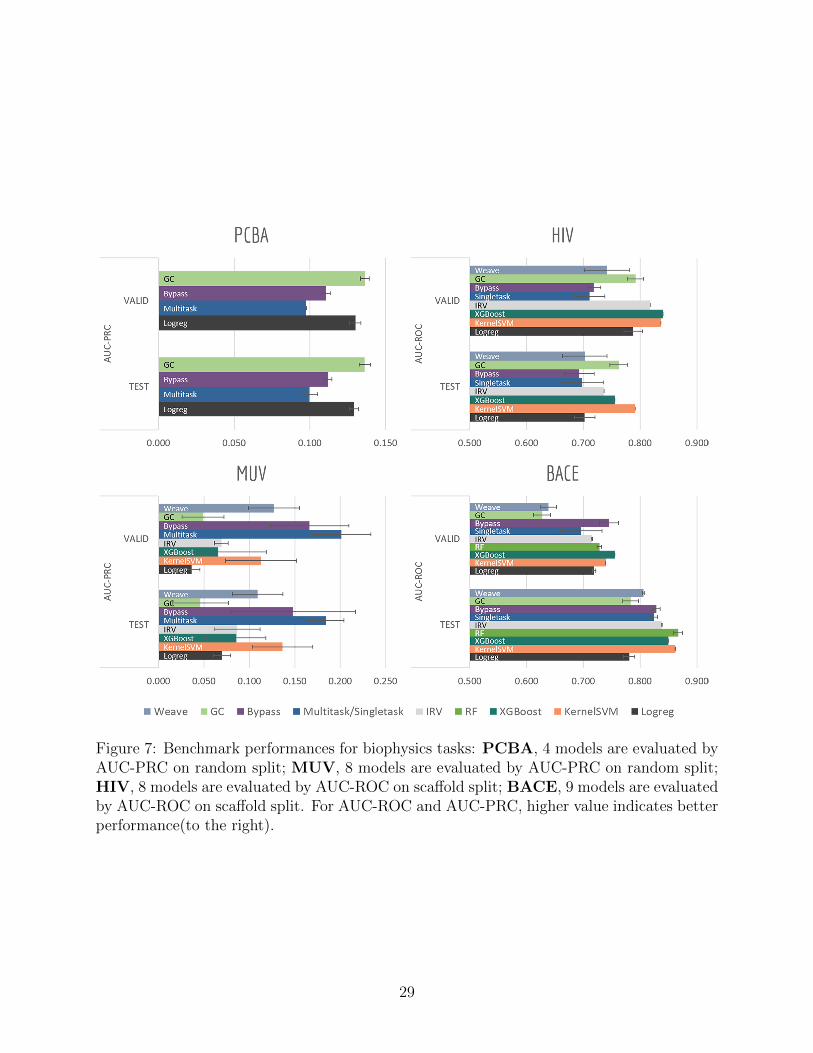
Figure 7: Benchmark performances for biophysics tasks: PCBA, 4 models are evaluated byAUC-PRC on random split; MUV, 8 models are evaluated by AUC-PRC on random split;HIV, 8 models are evaluated by AUC-ROC on scaffold split; BACE, 9 models are evaluatedby AUC-ROC on scaffold split. For AUC-ROC and AUC-PRC, higher value indicates betterperformance(to the right).

29

Figure 8: Benchmark performances for physiology tasks: ToxCast, 8 models are evaluatedby AUC-ROC on random split; Tox21, 9 models are evaluated by AUC-ROC on randomsplit; BBBP, 9 models are evaluated by AUC-ROC on scaffold split; SIDER, 9 modelsare evaluated by AUC-ROC on random split. For AUC-ROC, higher value indicates betterperformance(to the right).

30

Figure 9: Benchmark performances for physiology tasks: ClinTox, 9 models are evaluatedby AUC-ROC on random split.

Physiology and Biophysics Tasks

Tables 5, 6 and Figures 7, 8, 9 report AUC-ROC or AUC-PRC results of 4 to 9 different

models on biophysics datasets (PCBA, MUV, HIV, BACE) and physiology datasets (BBBP,

Tox21, Toxcast, SIDER, ClinTox). Some models were too computationally expensive to be

run on the larger datasets. All of these datasets contain only classification tasks.

Most models have train scores (listed in Tables 5, 6) higher than validation/test scores,

indicating that overfitting is a general issue. Singletask logistic regression exhibits the largest

gaps between train scores and validation/test scores, while models incorporating multitask

structure generally show less overfit, suggesting that multitask training has a regularizing

effect. Most physiological and biophysical datasets in MoleculeNet have only a low volume

of data for each task. Multitask algorithms combine different tasks, resulting in a larger pool

of data for model training. In particular, multitask training can, to some extent, compensate

for the limited data amount available for each individual task.

Graph convolutional models and weave models, each based on an adaptive method of

featurization,22,23 show strong validation/test results on larger datasets, along with less over-

31

fit. Similar results are reported in previous graph-based algorithms,14,19,22,23,76 showing that

learnable featurizations can provide a large boost compared with conventional featurizations.

For smaller singletask datasets (less than 3000 samples), differences between models are

less clear. Kernel SVM and ensemble tree methods (gradient boosting and random forests)

are more robust under data scarcity, while they generally need longer running time (see

Table 4). Worse performances of graph-based models are within expectation as complex

models generally require more training data.

Bypass networks show higher train scores and equal or higher validation/test scores

compared with vanilla multitask networks, suggesting that the bypass structure does add

robustness. IRV models achieve performance broadly comparable with multitask networks.

However, the quadratic nearest neighbor search makes the IRV models slower to train than

the multitask networks (see Table 4).

Three datasets (HIV, BACE, BBBP) in these two categories are evaluated under scaf-

fold splitting. As compounds are divided by their molecular scaffolds, increasing differ-

ences between train, validation and test performances are observed. Scaffold splits provide

a stronger test of a given model’s generalizability compared with random splitting. Two

datasets (PCBA, MUV) are evaluated by AUC-PRC, which is more practically useful under

high class imbalance as discussed above. Graph convolutional model performs the best on

PCBA (positive rate 1.40%), while results on MUV (positive rate 0.20%) are much less sta-

ble, which is most likely due to its extreme low amount of positive samples. Under such high

imbalance, graph-based models are still not robust enough in controlling false positives.

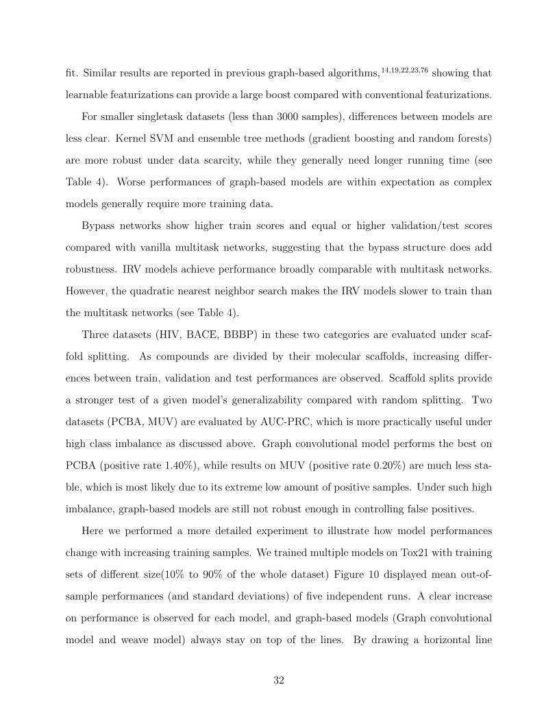
Here we performed a more detailed experiment to illustrate how model performances

change with increasing training samples. We trained multiple models on Tox21 with training

sets of different size(10% to 90% of the whole dataset) Figure 10 displayed mean out-of-

sample performances (and standard deviations) of five independent runs. A clear increase

on performance is observed for each model, and graph-based models (Graph convolutional

model and weave model) always stay on top of the lines. By drawing a horizontal line

32

Figure 10: Out-of-sample performances with different training set sizes on Tox21. Eachdatapoint is the average of 5 independent runs, with standard deviations shown as errorbars.

33

at around 0.80, we can see graph-based models achieve the similar level of accuracy with

multitask networks by using only one-third of the training samples(30% versus 90%).

Biophysics Task - PDBbind

The PDBBind dataset maps distinct ligand-protein structures to their binding affinities.

As discussed in the datasets section, we created grid featurizer to harness the joint ligand-

protein structural information in PDBBind to build a model that predicts the experimental

Ki of binding. We applied time splitting to all three subsets: core, refined, and full subsets

of PDBbind(Core contains roughly 200 structures, refined 4000, and full 15000. The smaller

datasets are cleaned more thoroughly than larger datasets.), with all results displayed in

Table 7 and Figure 11. Clearly as dataset size increased, we can see a significant boost on

validation/test set performances. At the same time, for the two larger subsets: refined and

full, switching from pure ligand-based ECFP to grid featurizer do increase the performances

by a small margin in both Singletask networks and random forests. While for core subset, all

models are showing relatively high errors and two featurizations do not show clear differences,

which is within expectation as sample amount in core subset is too small to support a stable

model performance. Note that models on the full set aren’t significantly superior to models

with less data; this effect may be due to the additional data being less clean.

Note that all models display heavy overfitting. Additional clean data may be required to

create more accurate models for protein-ligand binding.

Physical Chemistry Tasks

Solubility, solvation free energy and lipophilicity are basic physical chemistry properties

important for understanding how molecules interact with solvents. Figure 13 and Table 8

presented performances on predicting these properties.

Graph-based methods: graph convolutional model, DAG, MPNN and weave model all ex-

hibit significant boosts over vanilla singletask network, indicating the advantages of learnable

34

Figure 11: Benchmark performances of PDBbind: 5 models are evaluated by RMSE onthe three subsets: core, refined and full. Time split is applied to all three subsets. Noe thatfor RMSE, lower value indicates better performance(to the right).

35

featurizations. Differences between graph-based methods are rather minor and task-specific.

The best-performing models in this category can already reach the accuracy level of ab-initio

predictions(+/- 0.5 for ESOL, +/- 1.5 kcal/mol for FreeSolv).

We performed a more detailed comparison between data-driven methods and ab-initio

calculations on FreeSolv. Hydration free energy has been widely used as a test of compu-

tational chemistry methods. With free energy values ranging from −25.5 to 3.4 kcal/mol

in the FreeSolv dataset, RMSE for calculated results reached up to 1.5 kcal/mol.15 On the

other hand, though machine learning methods typically need large amounts of training data

to acquire predictive power, they can achieve higher accuracies given enough data. We in-

vestigated how the performance of machine learning methods on FreeSolv changes with the

volume of training data. In particular, we want to know the amount of data required for

machine learning to achieve accuracy similar to that of physically inspired algorithms.

Figure 12: Out-of-sample performances with different training set sizes on FreeSolv. Eachdatapoint is the average of 5 independent runs, with standard deviations shown as errorbars.

36

For Figure 12, we similarly generated a series of models with different training set vol-

umes and calculated their out-of-sample RMSE. Each data point displayed is the average of

5 independent runs, with standard deviations displayed as error bars. Both graph convo-

lutional model and weave model are capable of achieving better performances with enough

training samples (50% and 30% of the data respectively). Given the size of FreeSolv dataset

is only around 600 compounds, a weave model can reach state-of-the-art free energy calcu-

lation performances by training on merely 200 samples. On the other hand, comparing with

singletask network’s performance, weave model achieved the same level of accuracy with only

one-third of the training samples.

Quantum Mechanics Tasks

The QM datasets (QM7, QM7b, QM8, QM9) represent another distinct category of prop-

erties that are typically calculated through solving Schrodinger’s equation (approximately

using techniques such as DFT). As most conventional methods are slower than data-driven

methods by orders of magnitude, we hope to learn effective approximators by training on

existing datasets.

Table 9 and Figure 14 display the performances in mean absolute error of multiple meth-

ods. Table 10, 11 and 12 show detailed performances for each task.(Due to difference in

range of labels, mean performances of QM7b and QM9 are more skewed) Unsurprisingly,

significant boosts on performances and less overfitting are observed for models incorporat-

ing distance information (multitask networks and KRR with Coulomb Matrix featurization,

ANI-1, DTNN, MPNN). In particular, KRR and multitask networks(CM) outperform their

corresponding baseline models in QM7 and QM9 by a large margin, while ANI-1, DTNN and

MPNN display less error comparing with graph convolutional models as well. At the same

time, graph-based methods gain better performances than multitask networks and KRR

(CM) on most tasks. Table 10 shows that DTNN outperforms KRR(CM) on 12/14 tasks in

QM7b(Though the mean error shows the opposite result due to averaging errors on different

37

Figure 13: Benchmark performances for physical chemistry tasks: ESOL, 8 models areevaluated by RMSE on random split; FreeSolv, 8 models are evaluated by RMSE on randomsplit; Lipophilicity, 8 models are evaluated by RMSE on random split. Note that for RMSE,lower value indicates better performance(to the right).

38

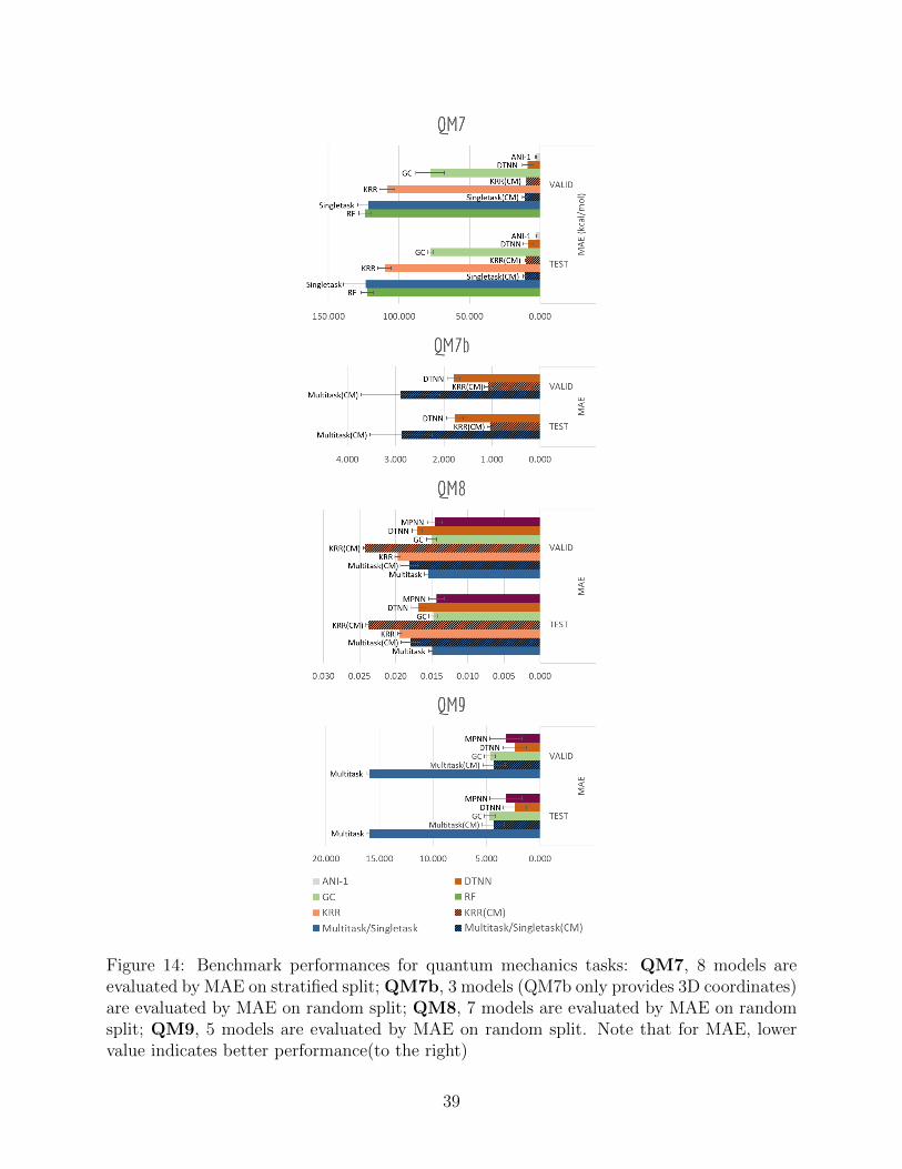
Figure 14: Benchmark performances for quantum mechanics tasks: QM7, 8 models areevaluated by MAE on stratified split; QM7b, 3 models (QM7b only provides 3D coordinates)are evaluated by MAE on random split; QM8, 7 models are evaluated by MAE on randomsplit; QM9, 5 models are evaluated by MAE on random split. Note that for MAE, lowervalue indicates better performance(to the right)

39

magnitudes). In total, ANI-1, DTNN and MPNN covered the best-performing models on

28/39 of all tasks in this category, again reflecting the superiority of learnable featurization.

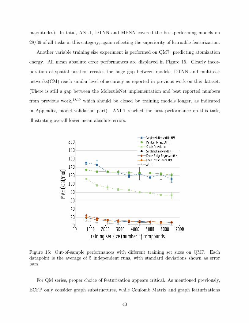
Another variable training size experiment is performed on QM7: predicting atomization

energy. All mean absolute error performances are displayed in Figure 15. Clearly incor-

poration of spatial position creates the huge gap between models, DTNN and multitask

networks(CM) reach similar level of accuracy as reported in previous work on this dataset.

(There is still a gap between the MoleculeNet implementation and best reported numbers

from previous work,18,19 which should be closed by training models longer, as indicated

in Appendix, model validation part). ANI-1 reached the best performance on this task,

illustrating overall lower mean absolute errors.

Figure 15: Out-of-sample performances with different training set sizes on QM7. Eachdatapoint is the average of 5 independent runs, with standard deviations shown as errorbars.

For QM series, proper choice of featurization appears critical. As mentioned previously,

ECFP only consider graph substructures, while Coulomb Matrix and graph featurizations

40

used by ANI-1, DTNN and MPNN are explicitly calculated on charges and physical distances,

which are exactly the required inputs for solving Schrodinger’s equation.

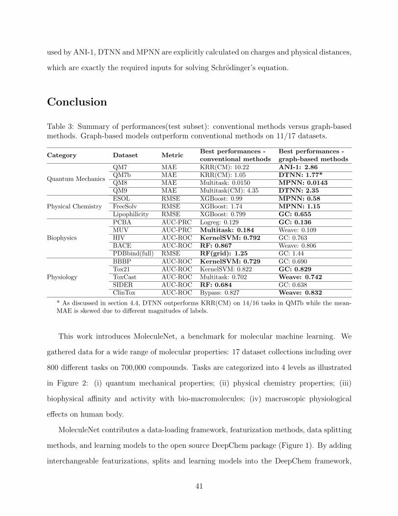
Conclusion

Table 3: Summary of performances(test subset): conventional methods versus graph-basedmethods. Graph-based models outperform conventional methods on 11/17 datasets.

Category Dataset MetricBest performances - Best performances -conventional methods graph-based methods

Quantum Mechanics

QM7 MAE KRR(CM): 10.22 ANI-1: 2.86QM7b MAE KRR(CM): 1.05 DTNN: 1.77*QM8 MAE Multitask: 0.0150 MPNN: 0.0143QM9 MAE Multitask(CM): 4.35 DTNN: 2.35

Physical ChemistryESOL RMSE XGBoost: 0.99 MPNN: 0.58FreeSolv RMSE XGBoost: 1.74 MPNN: 1.15Lipophilicity RMSE XGBoost: 0.799 GC: 0.655

Biophysics

PCBA AUC-PRC Logreg: 0.129 GC: 0.136MUV AUC-PRC Multitask: 0.184 Weave: 0.109HIV AUC-ROC KernelSVM: 0.792 GC: 0.763BACE AUC-ROC RF: 0.867 Weave: 0.806PDBbind(full) RMSE RF(grid): 1.25 GC: 1.44

Physiology

BBBP AUC-ROC KernelSVM: 0.729 GC: 0.690Tox21 AUC-ROC KernelSVM: 0.822 GC: 0.829ToxCast AUC-ROC Multitask: 0.702 Weave: 0.742SIDER AUC-ROC RF: 0.684 GC: 0.638ClinTox AUC-ROC Bypass: 0.827 Weave: 0.832

* As discussed in section 4.4, DTNN outperforms KRR(CM) on 14/16 tasks in QM7b while the mean-MAE is skewed due to different magnitudes of labels.

This work introduces MoleculeNet, a benchmark for molecular machine learning. We

gathered data for a wide range of molecular properties: 17 dataset collections including over

800 different tasks on 700,000 compounds. Tasks are categorized into 4 levels as illustrated

in Figure 2: (i) quantum mechanical properties; (ii) physical chemistry properties; (iii)

biophysical affinity and activity with bio-macromolecules; (iv) macroscopic physiological

effects on human body.

MoleculeNet contributes a data-loading framework, featurization methods, data splitting

methods, and learning models to the open source DeepChem package (Figure 1). By adding

interchangeable featurizations, splits and learning models into the DeepChem framework,

41

we can apply these primitives to the wide range of datasets in MoleculeNet.

Broadly, our results show that graph-based models outperformed other methods by com-

fortable margins on most datasets(11/17, best performances comparison in Table 3), reveal-

ing a clear advantage of learnable featurizations. However, this effect has some caveats:

Graph-based methods are not robust enough on complex tasks under data scarcity; on heav-

ily imbalanced classification datasets, conventional methods such as kernel SVM outperform

learnable featurizations with respect to recall of positives. Furthermore, for the PDBBind

and quantum mechanics datasets, the use of appropriate featurizations which contain per-

tinent information is very significant. Comparing fully connected neural networks, random

forests, and other comparatively simple algorithms, we claim that the PDBbind and QM7

results emphasize the necessity of using specialized features for different tasks. DTNN and

MPNN which use distance information perform better on QM datasets than simple graph

convolutions. While out of the scope of this paper, we note similarly that customized deep

learning algorithms12 could in principle supplant the need for hand-derived, specialized fea-

tures in such biophysical settings. On the FreeSolv dataset, comparison between conventional

ab-initio calculations and graph-based models for the prediction of solvation energies shows

that data-driven methods can outperform physical algorithms with moderate amounts of

data. These results suggest that data-driven physical chemistry will become increasingly im-

portant as methods mature. Results for biophysical and physiological datasets are currently

weaker than for other datasets, suggesting that better featurizations or more data may be

required for data-driven physiology to become broadly useful.

By providing a uniform platform for comparison and evaluation, we hope MoleculeNet

will facilitate the development of new methods for both chemistry and machine learning. In

future work, we hope to extend MoleculeNet to cover a broader range of molecular properties

than considered here. For example, 3D protein structure prediction, or DNA topological

modeling would benefit from the presence of strong benchmarks to encourage algorithmic

development. We hope that the open-source design of MoleculeNet will encourage researchers

42

to contribute implementations of other novel algorithms to the benchmark suite. In time,

we hope to see MoleculeNet grow into a comprehensive resource for the molecular machine

learning community.

Acknowledgement

We would like to thank the Stanford Computing Resources for providing us with access to

the Sherlock and Xstream GPU nodes. Thanks to Steven Kearnes and Patrick Riley for

early discussions about the MoleculeNet concept. Thanks to Aarthi Ramsundar for help

with diagram construction.

Thanks to Zheng Xu for feedback on the MoleculeNet API. Thanks to Patrick Hop for

contribution of the Lipophilicity dataset to MoleculeNet. Thanks to Anthony Gitter and

Johnny Israeli for suggesting the addition of AuPRC for imbalanced datasets.

The Pande Group is broadly supported by grants from the NIH (R01 GM062868 and

U19 AI109662) as well as gift funds and contributions from Folding@home donors.

We acknowledge the generous support of Dr. Anders G. Frøseth and Mr. Christian Sundt

for our work on machine learning.

B.R. was supported by the Fannie and John Hertz Foundation.

Appendix

Model Training and Hyperparameter Optimization

All models were trained on Stanford’s GPU clusters via DeepChem. No model was allowed

to train for more than 10 hours(time profile in Table 4. Users can reproduce benchmarks

locally by following directions from DeepChem.

Hyperparameters were determined using Gaussian Process Optimization via pyGPGO

(https://github.com/hawk31/pyGPGO), with max number of iterations set to 20. Opti-

43

mized hyperparameters for each model are listed, detailed hyperparameters can be found on

Deepchem.

Logistic Regression (Logreg)

• Learning rate

• L2 regularization

• Batch size

Support Vector Classification (KernelSVM)

• Penalty parameter C

• Kernel coefficient gamma for radial basis function

Kernel Ridge Regression (KRR)

• Penalty parameter

Random Forest (RF)

• Number of trees in the forest: 500

Gradient Boosting (XGBoost)

• Maximum tree depth

• Learning rate

• Number of boosted tree

44

Multitask/Singletask Networks

• Layer size

• Weight - initial standard deviation

• Bias - initial constant

• Learning rate


• Batch size

Bypass Networks

• Layer size(main layer and bypass layer)

• Weight - initial standard deviation(main layer and bypass layer)

• Bias - initial constant(main layer and bypass layer)

• Learning rate


• Batch size

Influence Relevance Voting (IRV)

• K(number of nearest neighbors)

• Learning rate

• Batch size

45

Graph Convolutional models (GC)

• Layer size of convolutional layers

• Layer size of fully-connected layer

• Learning rate

• Batch size

Weave models

• Length of output features(layer size) of convolutional layers

• Learning rate

• Batch size

Deep Tensor Neural Networks (DTNN)

• Length of atom embedding(features)

• Size of distance bin(from -1A to 19A)

• Learning rate

• Batch size

Directed Acyclic Graph models (DAG)

• Length of features in the convolutional layer

• Maximum number of propagation of a graph

• Learning rate

• Batch size

46

Message Passing Neural Networks (MPNN)

• Number of message passing phases

• Number of steps(iterations) in readout phase

• Learning rate

• Batch size

ANI-1

• Layer size

• Length of radial and angular symmetry functions

• Learning rate

• Batch size

All final performances were run three times with different fixed numerical seeds on the

best-performing hyperparameters, and data splitting methods have been set to maintain de-

termistic behavior. These settings control most randomness in learning process, but bench-

mark runs(on the same seed) may vary on the order of 1% due to other sources of nonde-

terminism. Mean and standard deviations of all results are presented in the Performances

section of Appendix.

We measured model running time of Tox21, MUV, QM8 and Lipophicility on a single

node in Stanford’s GPU clusters(CPU: Intel Xeon E5-2640 v3 @2.60 GHz, GPU: NVIDIA

Tesla K80), results listed below:

47

Table 4: Time Profile for Tox21, MUV, QM8 and Lipophilic-ity(second)

Model Tox21 MUV QM8 Lipophilicity

Logreg 93 522

KernelSVM 2574 2231

KRR 3390/5153* 24

RF 24273 186

XGBoost 2082 2418 410

Multitask/Singletask 22 858 275/701* 21

Bypass 31 938

IRV 58 2674

GC 246 2320 512 131

Weave 323 4593 255

DAG 5142

DTNN 940

MPNN 3383 1626

* ECFP/Coulomb Matrix

48

Performances

Table 5: PCBA, MUV, HIV and BACE Performances: AUC-PRC for PCBA and MUV,AUC-ROC for HIV and BACE

Model Model Training Validation Test

PCBA

Logreg 0.166± 0.001 0.130± 0.004 0.129± 0.003Multitask 0.100± 0.003 0.097± 0.000 0.100± 0.006

Bypass 0.121± 0.001 0.111± 0.003 0.112± 0.002GC 0.151± 0.001 0.136± 0.003 0.136± 0.004

MUV

Logreg 0.238± 0.010 0.036± 0.009 0.070± 0.009KernelSVM 0.922± 0.034 0.113± 0.039 0.137± 0.033XGBoost 0.159± 0.018 0.066± 0.053 0.086± 0.033

IRV 0.043± 0.006 0.069± 0.008 0.087± 0.025Multitask 0.385± 0.014 0.202± 0.032 0.184± 0.020

Bypass 0.317± 0.027 0.166± 0.043 0.148± 0.069GC 0.040± 0.013 0.049± 0.023 0.046± 0.031

Weave 0.060± 0.030 0.127± 0.028 0.109± 0.028

HIV


IRV 0.849± 0.000 0.818± 0.000 0.737± 0.000Multitask 0.753± 0.012 0.711± 0.027 0.698± 0.037

Bypass 0.736± 0.017 0.719± 0.012 0.693± 0.026GC 0.903± 0.004 0.792± 0.014 0.763± 0.016

Weave 0.725± 0.004 0.742± 0.040 0.703± 0.039

BACE


RF 0.999± 0.000 0.728± 0.004 0.867± 0.008IRV 0.887± 0.000 0.715± 0.001 0.838± 0.000

Multitask 0.863± 0.034 0.696± 0.037 0.824± 0.006Bypass 0.931± 0.001 0.745± 0.017 0.829± 0.006

GC 0.852± 0.046 0.627± 0.015 0.783± 0.014Weave 0.862± 0.009 0.638± 0.014 0.806± 0.002

49

Table 6: BBBP, Tox21, ToxCast, SIDER, ClinTox Performances (AUC-ROC)


BBBP


RF 1.000± 0.000 0.956± 0.002 0.714± 0.000IRV 0.915± 0.000 0.964± 0.000 0.700± 0.000


GC 0.956± 0.004 0.943± 0.002 0.690± 0.009Weave 0.873± 0.010 0.951± 0.005 0.671± 0.014

Tox21


RF 0.999± 0.000 0.763± 0.002 0.769± 0.015IRV 0.805± 0.003 0.807± 0.006 0.799± 0.006


GC 0.905± 0.004 0.825± 0.013 0.829± 0.006Weave 0.875± 0.004 0.828± 0.008 0.820± 0.010

ToxCast


IRV 0.663± 0.004 0.660± 0.009 0.663± 0.015Multitask 0.887± 0.002 0.705± 0.017 0.702± 0.013

Bypass 0.793± 0.002 0.684± 0.016 0.676± 0.005GC 0.815± 0.003 0.709± 0.013 0.716± 0.014

Weave 0.830± 0.006 0.750± 0.007 0.742± 0.003

SIDER


RF 1.000± 0.000 0.650± 0.013 0.684± 0.009IRV 0.628± 0.004 0.657± 0.028 0.640± 0.020


GC 0.735± 0.013 0.609± 0.021 0.638± 0.012Weave 0.647± 0.015 0.591± 0.031 0.581± 0.027

ClinTox


RF 0.996± 0.001 0.688± 0.107 0.713± 0.056IRV 0.804± 0.004 0.748± 0.075 0.770± 0.072


GC 0.962± 0.005 0.920± 0.035 0.807± 0.047Weave 0.948± 0.013 0.875± 0.066 0.832± 0.037

50

Table 7: PDBbind Performances (Root-Mean-Square Error)


PDBbind - core

RF 0.82± 0.00 2.02± 0.02 2.03± 0.01RF(grid) 0.73± 0.01 1.98± 0.01 2.27± 0.01Multitask 1.62± 0.03 1.86± 0.01 2.21± 0.02

Multitask(grid) 1.51± 0.05 1.92± 0.02 2.20± 0.03GC 1.42± 0.04 2.10± 0.05 1.92± 0.07

PDBbind - refined



PDBbind - full



Table 8: ESOL, FreeSolv, Lipophilicity Performances (Root-Mean-Square Error)


ESOL

RF 0.51± 0.01 1.16± 0.15 1.07± 0.19Multitask 0.59± 0.04 1.17± 0.13 1.12± 0.15XGBoost 0.51± 0.08 1.05± 0.10 0.99± 0.14

KRR 0.38± 0.01 1.65± 0.19 1.53± 0.06GC 0.43± 0.20 1.05± 0.15 0.97± 0.01

DAG 0.32± 0.03 0.74± 0.04 0.82± 0.08Weave 0.34± 0.04 0.57± 0.04 0.61± 0.07MPNN 0.25± 0.06 0.55± 0.02 0.58± 0.03

FreeSolv


KRR 0.31± 0.03 2.10± 0.12 2.11± 0.07GC 0.31± 0.09 1.35± 0.15 1.40± 0.16

DAG 0.49± 0.46 1.48± 0.15 1.63± 0.18Weave 0.32± 0.04 1.19± 0.08 1.22± 0.28MPNN 0.31± 0.05 1.20± 0.02 1.15± 0.12

Lipophilicity


KRR 0.180± 0.002 0.889± 0.009 0.899± 0.043GC 0.471± 0.001 0.678± 0.040 0.655± 0.036

DAG 0.173± 0.026 0.857± 0.050 0.835± 0.039Weave 0.549± 0.051 0.734± 0.011 0.715± 0.035MPNN 0.363± 0.043 0.757± 0.030 0.719± 0.031

51

Table 9: QM7, QM7b, QM8 and QM9 Performances (Mean Absolute Error)


QM7

RF 47.1± 0.1 124.0± 4.6 122.7± 4.2Multitask 101.8± 13.7 121.7± 7.5 123.7± 15.6

KRR 65.5± 0.3 108.3± 5.4 110.3± 4.7GC 67.8± 4.0 77.9± 10.0 77.9± 2.1

Multitask(CM) 10.4± 1.8 11.0± 1.7 10.8± 1.3KRR(CM) 0.1± 0.0 9.9± 0.1 10.2± 0.3

DTNN 8.2± 3.9 8.9± 3.7 8.8± 3.5ANI-1 2.42± 0.32 2.99± 0.22 2.86± 0.25

QM7bMultitask(CM) 2.95± 0.70 2.90± 0.82 2.89± 0.65

KRR(CM) 0.01± 0.00 1.08± 0.08 1.05± 0.06DTNN 1.68± 0.18 1.79± 0.14 1.77± 0.17

QM8

Multitask 0.0081± 0.0002 0.0155± 0.0005 0.0150± 0.0005KRR 0.0152± 0.0001 0.0197± 0.0004 0.0195± 0.0003GC 0.0123± 0.0009 0.0150± 0.0006 0.0148± 0.0006

Multitask(CM) 0.0163± 0.0010 0.0181± 0.0012 0.0179± 0.0013KRR(CM) 0.0002± 0.0000 0.0242± 0.0003 0.0238± 0.0004

DTNN 0.0140± 0.0009 0.0170± 0.0007 0.0169± 0.0009MPNN 0.0128± 0.0010 0.0146± 0.0010 0.0143± 0.0011

QM9

Multitask 15.3± 0.2 15.9± 0.2 16.0± 0.2GC 4.6± 0.5 4.7± 0.5 4.7± 0.5

Multitask(CM) 4.3± 1.0 4.3± 1.1 4.4± 1.0DTNN 2.3± 1.1 2.4± 1.1 2.4± 1.1MPNN 3.2± 1.5 3.2± 1.5 3.2± 1.5

Table 10: QM7b Test Set Performances of All Tasks(Mean Absolute Error)

Task Multitask(CM) KRR(CM) DTNN

Atomization energy - PBE0 36.0 9.3 21.5

Excitation energy of maximal optimal absorption - ZINDO 1.31 1.83 1.26

Highest absorption - ZINDO 0.086 0.098 0.074

HOMO - ZINDO 0.293 0.369 0.192

LUMO - ZINDO 0.255 0.361 0.159

1st excitation energy - ZINDO 0.368 0.479 0.296

Ionization potential - ZINDO 0.305 0.408 0.214

Electron Affinity - ZINDO 0.271 0.404 0.174

HOMO - KS 0.247 0.272 0.155

LUMO - KS 0.187 0.239 0.129

HOMO - GW 0.270 0.294 0.166

LUMO - GW 0.172 0.236 0.139

Polarizability - PBE0 0.335 0.225 0.173

Polarizability - SCS 0.317 0.116 0.149

52

Table 11: QM8 Test Set Performances of All Tasks(Mean Absolute Error)

Task Multitask GC KRR Multitask(CM) KRR(CM) DTNN MPNN

E1 - CC2 0.0088 0.0074 0.0115 0.0125 0.0137 0.0092 0.0084

E2 - CC2 0.0098 0.0085 0.0116 0.0114 0.0124 0.0092 0.0091

f1 - CC2 0.0145 0.0175 0.0202 0.0186 0.0272 0.0182 0.0151

f2 - CC2 0.0320 0.0328 0.0387 0.0358 0.0460 0.0377 0.0314

E1 - PBE0 0.0089 0.0076 0.0118 0.0126 0.0140 0.0090 0.0083

E2 - PBE0 0.0096 0.0083 0.0117 0.0114 0.0122 0.0086 0.0086

f1 - PBE0 0.0121 0.0125 0.0189 0.0152 0.0258 0.0155 0.0123

f2 - PBE0 0.0252 0.0246 0.0319 0.0267 0.0376 0.0281 0.0236

E1 - CAM 0.0083 0.0070 0.0111 0.0119 0.0132 0.0086 0.0079

E2 - CAM 0.0090 0.0076 0.0109 0.0106 0.0115 0.0082 0.0082

f1 - CAM 0.0140 0.0153 0.0208 0.0177 0.0304 0.0180 0.0134

f2 - CAM 0.0274 0.0285 0.0345 0.0303 0.0417 0.0322 0.0258

Table 12: QM9 Test Set Performances of All Tasks(Mean Absolute Error)

Task Multitask Multitask(CM) GC DTNN MPNN

mu 0.602 0.519 0.583 0.244 0.358

alpha 3.10 0.85 1.37 0.95 0.89

HOMO 0.00660 0.00506 0.00716 0.00388 0.00541

LUMO 0.00854 0.00645 0.00921 0.00513 0.00623

gap 0.0100 0.0086 0.0112 0.0066 0.0082

R2 125.7 46.0 35.9 17.0 28.5

ZPVE 0.01109 0.00207 0.00299 0.00172 0.00216

U0 15.10 2.27 3.41 2.43 2.05

U 15.10 2.27 3.41 2.43 2.00

H 15.10 2.27 3.41 2.43 2.02

G 15.10 2.27 3.41 2.43 2.02

Cv 1.77 0.39 0.65 0.27 0.42

Grid Featurizer

In our implementation, we generate a vector with length 2052 for each pair of ligand and

protein. Detailed process listed below:

First, binding pocket atoms of the protein are extracted using a distance cutoff of 4.5 A.

In this process, atom in the protein will be extracted only if it locates within this distance

from any atom in the ligand molecule.

Intra-ligand and intra-protein fingerprints are generated (using the ordinary circular fin-

53

gerprint with radius of 2) respectively on the atoms from the ligand and atoms in the binding

pocket of the protein, and then hashed together to form a vector of length 512.

Then we form three different sets of contacting atom pairs between ligand and protein,

whose intra-pair distance falls within bins: 0 ∼ 2 A, 2 ∼ 3 Aand 3 ∼ 4.5 A. Each set of pairs

is hashed into a fixed length fingerprint with length 512.

Finally, salt bridges are counted, hydrogen bonds are counted in three different distance

bins, forming the last four digits. In total the fingerprints have length of 2052.

ClinTox

The ClinTox dataset addresses clinical drug toxicity by providing a qualitative comparison of

drugs approved by the FDA and those that have failed clinical trials for toxicity reasons. We

compiled the FDA-approved drug names from annotations in the SWEETLEAD database.

We compiled the names of drugs that failed clinical trials for toxicity reasons from the

Aggregate Analysis of ClinicalTrials.gov (AACT) database. To identify these drug names,

we relied on annotations from the clinical study table titled ”clinical study noclob.txt” in

the AACT database. From this table, we selected clinical trials where the overall status was

”terminated,” ”suspended,” or ”withdrawn,” and the explanation for the status included the

terms ”adverse,” ”toxic,” or ”death.”

Dataset and model access

Table 13 listed DeepChem commands to load datasets and models in MoleculeNet. For more

detailed instructions please refer to the docs and examples. Tutorial for building customized

datasets can be found at https://github.com/deepchem/deepchem/blob/master/examples/

notebooks/dataset_preparation.ipynb

54

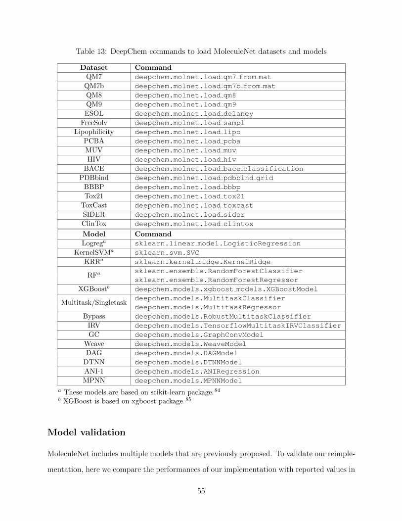
https://github.com/deepchem/deepchem/blob/master/examples/notebooks/dataset_preparation.ipynb

https://github.com/deepchem/deepchem/blob/master/examples/notebooks/dataset_preparation.ipynb

Table 13: DeepChem commands to load MoleculeNet datasets and models

Dataset Command

QM7 deepchem.molnet.load qm7 from matQM7b deepchem.molnet.load qm7b from matQM8 deepchem.molnet.load qm8QM9 deepchem.molnet.load qm9ESOL deepchem.molnet.load delaney

FreeSolv deepchem.molnet.load samplLipophilicity deepchem.molnet.load lipo

PCBA deepchem.molnet.load pcbaMUV deepchem.molnet.load muvHIV deepchem.molnet.load hiv

BACE deepchem.molnet.load bace classificationPDBbind deepchem.molnet.load pdbbind grid

BBBP deepchem.molnet.load bbbpTox21 deepchem.molnet.load tox21

ToxCast deepchem.molnet.load toxcastSIDER deepchem.molnet.load siderClinTox deepchem.molnet.load clintox

Model Command

Logrega sklearn.linear model.LogisticRegressionKernelSVMa sklearn.svm.SVC

KRRa sklearn.kernel ridge.KernelRidge

RFa sklearn.ensemble.RandomForestClassifiersklearn.ensemble.RandomForestRegressor

XGBoostb deepchem.models.xgboost models.XGBoostModel

Multitask/Singletaskdeepchem.models.MultitaskClassifierdeepchem.models.MultitaskRegressor

Bypass deepchem.models.RobustMultitaskClassifierIRV deepchem.models.TensorflowMultitaskIRVClassifierGC deepchem.models.GraphConvModel

Weave deepchem.models.WeaveModelDAG deepchem.models.DAGModel

DTNN deepchem.models.DTNNModelANI-1 deepchem.models.ANIRegressionMPNN deepchem.models.MPNNModel

a These models are based on scikit-learn package.84b XGBoost is based on xgboost package.85

Model validation

MoleculeNet includes multiple models that are previously proposed. To validate our reimple-

mentation, here we compare the performances of our implementation with reported values in

55

previous papers. All model validation scripts and trained models can be found in DeepChem.

Note that performances of our models might be different from values in the benchmark

tables due to no limitation imposed on running time(more epochs), different random splitting

patterns, etc.

Graph Convolutional models

We evaluate the model on ESOL dataset, note that we provide performances based on a

80/10/10 random train, valid, test splitting, while the original paper reported performance

under cross validation.22

RMSE in logS(log solubility in mol per litre):

• Original result: 0.52± 0.07

• Reimplementation: 0.39 for valid subset, 0.31 for test subset

Directed Acyclic Graph models

We evaluate the model on ESOL dataset with the same splitting pattern, the original paper

reported performance under 10-fold cross validation.14

RMSE in logS(log solubility in mol per litre):

• Original result: 0.58± 0.07


Weave models

We evaluate the model on Tox21 dataset, using 80/10/10 random train, valid, test splitting.

The original paper reported performance as median score of 5-fold cross validation.23

56

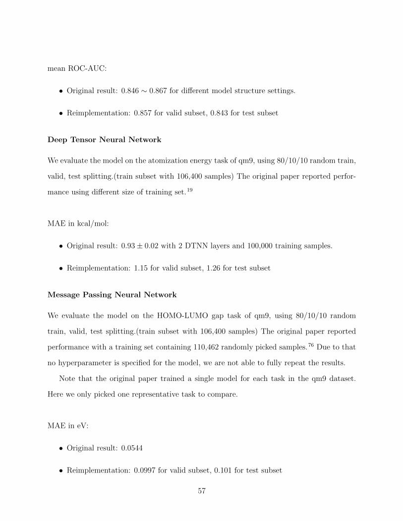
mean ROC-AUC:

• Original result: 0.846 ∼ 0.867 for different model structure settings.


Deep Tensor Neural Network

We evaluate the model on the atomization energy task of qm9, using 80/10/10 random train,

valid, test splitting.(train subset with 106,400 samples) The original paper reported perfor-

mance using different size of training set.19

MAE in kcal/mol:

• Original result: 0.93± 0.02 with 2 DTNN layers and 100,000 training samples.


Message Passing Neural Network

We evaluate the model on the HOMO-LUMO gap task of qm9, using 80/10/10 random

train, valid, test splitting.(train subset with 106,400 samples) The original paper reported

performance with a training set containing 110,462 randomly picked samples.76 Due to that

no hyperparameter is specified for the model, we are not able to fully repeat the results.

Note that the original paper trained a single model for each task in the qm9 dataset.

Here we only picked one representative task to compare.

MAE in eV:

• Original result: 0.0544


57

Influence Relevance Voting

We evaluate the model on the HIV dataset, using 80/10/10 random train, valid, test split-

ting. The original paper reported performance under 10-fold cross validation.75

ROC-AUC:

• Original result: 0.845


References

(1) Gasteiger, J.; Zupan, J. Angewandte Chemie International Edition 1993, 32, 503–527.

(2) Zupan, J.; Gasteiger, J. Neural networks in chemistry and drug design; John Wiley &

Sons, Inc., 1999.

(3) Varnek, A.; Baskin, I. Journal of chemical information and modeling 2012, 52, 1413–

1437.

(4) Mitchell, J. B. Wiley Interdisciplinary Reviews: Computational Molecular Science

2014, 4, 468–481.

(5) Devillers, J. Neural networks in QSAR and drug design; Academic Press, 1996.

(6) Schneider, G.; Wrede, P. Progress in biophysics and molecular biology 1998, 70, 175–

222.

(7) LeCun, Y.; Bengio, Y.; Hinton, G. Nature 2015, 521, 436–444.

(8) Schmidhuber, J. Neural networks 2015, 61, 85–117.

(9) Ma, J.; Sheridan, R. P.; Liaw, A.; Dahl, G. E.; Svetnik, V. Journal of chemical infor-

mation and modeling 2015, 55, 263–274.

58

(10) Ramsundar, B.; Kearnes, S.; Riley, P.; Webster, D.; Konerding, D.; Pande, V. arXiv

preprint arXiv:1502.02072 2015,

(11) Unterthiner, T.; Mayr, A.; unter Klambauer, G.; Steijaert, M.; Wenger, J.; Ceule-

mans, H.; Hochreiter, S. Deep Learning as an Opportunity in Virtual Screening. Deep

Learning and Representation Learning Workshop (NIPS 2014). 2014.

(12) Wallach, I.; Dzamba, M.; Heifets, A. arXiv preprint arXiv:1510.02855 2015,

(13) Delaney, J. S. Journal of Chemical Information and Modeling 2004, 44, 1000–1005.

(14) Lusci, A.; Pollastri, G.; Baldi, P. Journal of chemical information and modeling 2013,

53, 1563–1575.

(15) Mobley, D. L.; Wymer, K. L.; Lim, N. M.; Guthrie, J. P. Journal of Computer-Aided

Molecular Design 2014, 28, 135–150.

(16) Mobley, D. L.; Guthrie, J. P. Journal of Computer-Aided Molecular Design 2014, 28,

711–720.

(17) Rupp, M.; Tkatchenko, A.; Muller, K.-R.; Lilienfeld, O. A. v. Physical Review Letters

2012, 108, 058301.

(18) Montavon, G.; Rupp, M.; Gobre, V.; Vazquez-Mayagoitia, A.; Hansen, K.;

Tkatchenko, A.; Muller, K.-R.; Lilienfeld, O. A. v. New Journal of Physics 2013,

15, 095003.

(19) Schutt, K. T.; Arbabzadah, F.; Chmiela, S.; Muller, K. R.; Tkatchenko, A. arXiv

preprint arXiv:1609.08259 2016,

(20) McGibbon, R. T.; Taube, A. G.; Donchev, A. G.; Siva, K.; Hernandez, F.; Hargus, C.;

Law, K.-H.; Klepeis, J. L.; Shaw, D. E. The Journal of Chemical Physics 2017, 147,

161725.

59

(21) Rogers, D.; Hahn, M. Journal of Chemical Information and Modeling 2010, 50, 742–

754.

(22) Duvenaud, D.; Maclaurin, D.; Aguilera-Iparraguirre, J.; Gomez-Bombarelli, R.;

Hirzel, T.; Aspuru-Guzik, A.; Adams, R. P. arXiv preprint arXiv:1509.09292 2015,

(23) Kearnes, S.; McCloskey, K.; Berndl, M.; Pande, V.; Riley, P. arXiv preprint

arXiv:1603.00856 2016,

(24) Miller, G. A. Communications of the ACM 1995, 38, 39–41.

(25) Deng, J.; Dong, W.; Socher, R.; Li, L.-J.; Li, K.; Fei-Fei, L. ImageNet: A Large-Scale

Hierarchical Image Database. CVPR09. 2009.

(26) Russakovsky, O.; Deng, J.; Su, H.; Krause, J.; Satheesh, S.; Ma, S.; Huang, Z.; Karpa-

thy, A.; Khosla, A.; Bernstein, M.; Berg, A. C.; Fei-Fei, L. International Journal of

Computer Vision (IJCV) 2015, 115, 211–252.

(27) Krizhevsky, A.; Sutskever, I.; Hinton, G. E. ImageNet Classification with Deep Convo-

lutional Neural Networks. NIPS Proceedings. 2012.

(28) Szegedy, C.; Liu, W.; Jia, Y.; Sermanet, P.; Reed, S.; Anguelov, D.; Erhan, D.; Van-

houcke, V.; Rabinovich, A. arXiv preprint arXiv:1409.4842 2014,

(29) He, K.; Zhang, X.; Ren, S.; Sun, J. arXiv preprint arXiv:1512.03385 2015,

(30) DeepChem: Deep-learning models for Drug Discovery and Quantum Chemistry. https:

//github.com/deepchem/deepchem, Accessed: 2017-09-27.

(31) others,, et al. Journal of Machine Learning Research 2011, 12, 2825–2830.

(32) others,, et al. arXiv preprint arXiv:1603.04467 2016,

(33) Sheridan, R. P. Journal of chemical information and modeling 2013, 53, 783–790.

60

https://github.com/deepchem/deepchem

https://github.com/deepchem/deepchem

(34) Bolton, E. E.; Wang, Y.; Thiessen, P. A.; Bryant, S. H. Annual reports in computational

chemistry 2008, 4, 217–241.

(35) Wang, T.; Xiao, J.; Suzek, T. O.; Zhang, J.; Wang, J.; Zhou, Z.; Han, L.; Kara-

petyan, K.; Dracheva, S.; Shoemaker, B. A.; Bolton, E.; Gindulyte, A.; Bryant, S. H.

Nucleic Acids Research 2012, 40, D400–D412.

(36) Grazulis, S.; Chateigner, D.; Downs, R. T.; Yokochi, A.; Quiros, M.; Lutterotti, L.;

Manakova, E.; Butkus, J.; Moeck, P.; Le Bail, A. Journal of Applied Crystallography

2009, 42, 726–729.

(37) Groom, C. R.; Bruno, I. J.; Lightfoot, M. P.; Ward, S. C. Acta Crystallographica Section

B: Structural Science, Crystal Engineering and Materials 2016, 72, 171–179.

(38) Berman, H.; Henrick, K.; Nakamura, H. Nature Structural & Molecular Biology 2003,

10, 980–980.

(39) Quantum Machine. http://quantum-machine.org/datasets/, Accessed: 2017-09-27.

(40) Weininger, D. Journal of chemical information and computer sciences 1988, 28, 31–36.

(41) Blum, L. C.; Reymond, J.-L. Journal of the American Chemical Society 2009, 131,

8732–8733.

(42) Ramakrishnan, R.; Hartmann, M.; Tapavicza, E.; Lilienfeld, O. A. v. The Journal of

Chemical Physics 2015, 143, 084111.

(43) Ruddigkeit, L.; Deursen, R. v.; Blum, L. C.; Reymond, J.-L. Journal of Chemical

Information and Modeling 2012, 52, 2864–2875.

(44) Ramakrishnan, R.; Dral, P. O.; Rupp, M.; Lilienfeld, O. A. v. Scientific Data 2014, 1,

140022.

(45) Hersey, A. ChEMBL Deposited Data Set - AZ dataset ; 2015.

61

http://quantum-machine.org/datasets/

(46) Rohrer, S. G.; Baumann, K. Journal of Chemical Information and Modeling 2009, 49,

169–184.

(47) AIDS Antiviral Screen Data. https://wiki.nci.nih.gov/display/NCIDTPdata/

AIDS+Antiviral+Screen+Data, Accessed: 2017-09-27.

(48) Wang, R.; Fang, X.; Lu, Y.; Wang, S. Journal of Medicinal Chemistry 2004, 47, 2977–

2980.

(49) Wang, R.; Fang, X.; Lu, Y.; Yang, C.-Y.; Wang, S. Journal of Medicinal Chemistry

2005, 48, 4111–4119.

(50) Liu, Z.; Li, Y.; Han, L.; Li, J.; Liu, J.; Zhao, Z.; Nie, W.; Liu, Y.; Wang, R. Bioinfor-

matics 2014, 31, 405–412.

(51) Subramanian, G.; Ramsundar, B.; Pande, V.; Denny, R. A. Journal of Chemical Infor-

mation and Modeling 2016, 56, 1936–1949.

(52) Martins, I. F.; Teixeira, A. L.; Pinheiro, L.; Falcao, A. O. Journal of Chemical Infor-

mation and Modeling 2012, 52, 1686–1697.

(53) Tox21 Challenge. https://tripod.nih.gov/tox21/challenge/, Accessed: 2017-09-

27.

(54) Richard, A. M. et al. Chemical Research in Toxicology 2016, 29, 1225–1251.

(55) Kuhn, M.; Letunic, I.; Jensen, L. J.; Bork, P. Nucleic Acids Research 2016, 44, D1075–

D41079.

(56) Altae-Tran, H.; Ramsundar, B.; Pappu, A. S.; Pande, V. arXiv preprint

arXiv:1611.03199 2016,

(57) Medical Dictionary for Regulatory Activities. http://www.meddra.org/, Accessed:

2017-09-27.

62

https://wiki.nci.nih.gov/display/NCIDTPdata/AIDS+Antiviral+Screen+Data

https://wiki.nci.nih.gov/display/NCIDTPdata/AIDS+Antiviral+Screen+Data

https://tripod.nih.gov/tox21/challenge/

http://www.meddra.org/

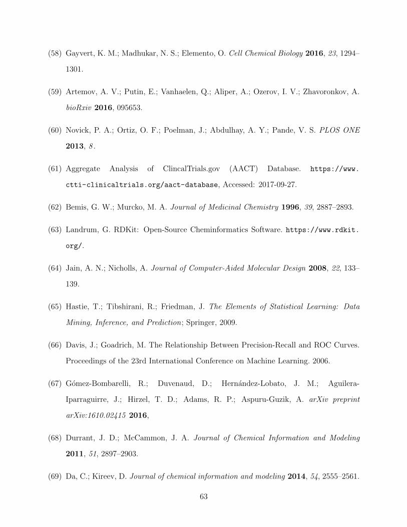
(58) Gayvert, K. M.; Madhukar, N. S.; Elemento, O. Cell Chemical Biology 2016, 23, 1294–

1301.

(59) Artemov, A. V.; Putin, E.; Vanhaelen, Q.; Aliper, A.; Ozerov, I. V.; Zhavoronkov, A.

bioRxiv 2016, 095653.

(60) Novick, P. A.; Ortiz, O. F.; Poelman, J.; Abdulhay, A. Y.; Pande, V. S. PLOS ONE

2013, 8 .

(61) Aggregate Analysis of ClincalTrials.gov (AACT) Database. https://www.

ctti-clinicaltrials.org/aact-database, Accessed: 2017-09-27.

(62) Bemis, G. W.; Murcko, M. A. Journal of Medicinal Chemistry 1996, 39, 2887–2893.

(63) Landrum, G. RDKit: Open-Source Cheminformatics Software. https://www.rdkit.

org/.

(64) Jain, A. N.; Nicholls, A. Journal of Computer-Aided Molecular Design 2008, 22, 133–

139.

(65) Hastie, T.; Tibshirani, R.; Friedman, J. The Elements of Statistical Learning: Data

Mining, Inference, and Prediction; Springer, 2009.

(66) Davis, J.; Goadrich, M. The Relationship Between Precision-Recall and ROC Curves.

Proceedings of the 23rd International Conference on Machine Learning. 2006.

(67) Gomez-Bombarelli, R.; Duvenaud, D.; Hernandez-Lobato, J. M.; Aguilera-

Iparraguirre, J.; Hirzel, T. D.; Adams, R. P.; Aspuru-Guzik, A. arXiv preprint

arXiv:1610.02415 2016,

(68) Durrant, J. D.; McCammon, J. A. Journal of Chemical Information and Modeling

2011, 51, 2897–2903.

(69) Da, C.; Kireev, D. Journal of chemical information and modeling 2014, 54, 2555–2561.

63

https://www.ctti-clinicaltrials.org/aact-database

https://www.ctti-clinicaltrials.org/aact-database

https://www.rdkit.org/

https://www.rdkit.org/

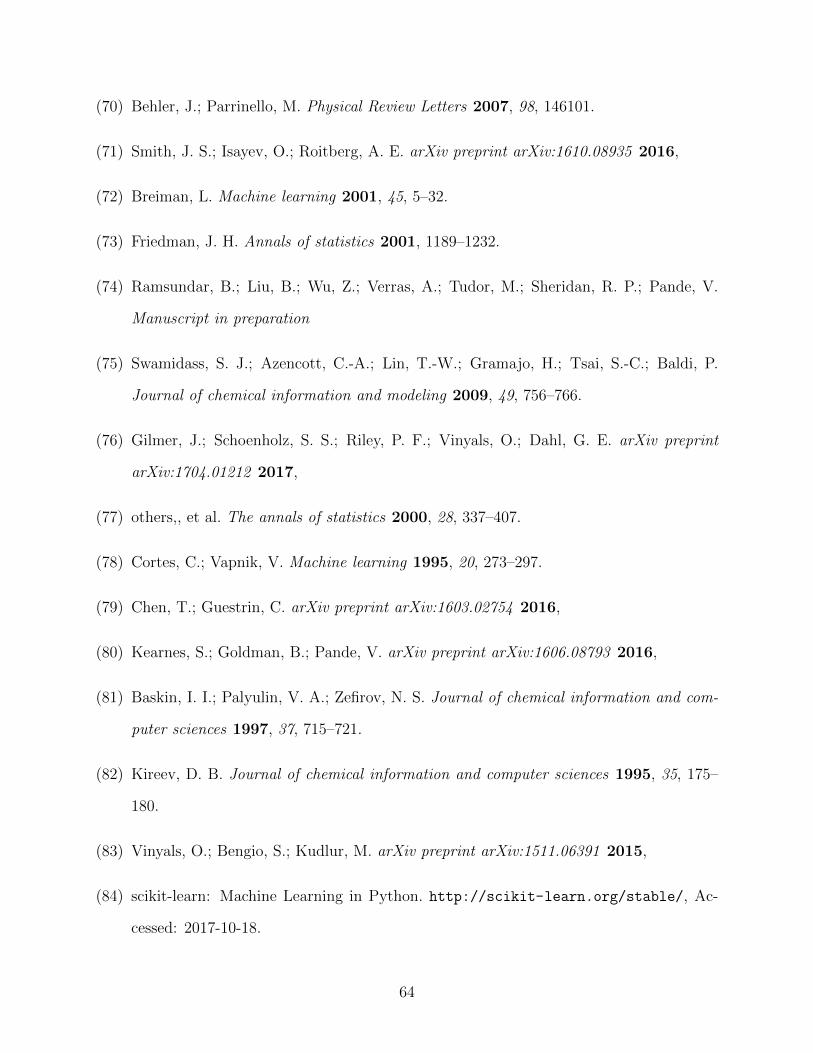
(70) Behler, J.; Parrinello, M. Physical Review Letters 2007, 98, 146101.

(71) Smith, J. S.; Isayev, O.; Roitberg, A. E. arXiv preprint arXiv:1610.08935 2016,

(72) Breiman, L. Machine learning 2001, 45, 5–32.

(73) Friedman, J. H. Annals of statistics 2001, 1189–1232.

(74) Ramsundar, B.; Liu, B.; Wu, Z.; Verras, A.; Tudor, M.; Sheridan, R. P.; Pande, V.

Manuscript in preparation

(75) Swamidass, S. J.; Azencott, C.-A.; Lin, T.-W.; Gramajo, H.; Tsai, S.-C.; Baldi, P.

Journal of chemical information and modeling 2009, 49, 756–766.

(76) Gilmer, J.; Schoenholz, S. S.; Riley, P. F.; Vinyals, O.; Dahl, G. E. arXiv preprint

arXiv:1704.01212 2017,

(77) others,, et al. The annals of statistics 2000, 28, 337–407.

(78) Cortes, C.; Vapnik, V. Machine learning 1995, 20, 273–297.

(79) Chen, T.; Guestrin, C. arXiv preprint arXiv:1603.02754 2016,

(80) Kearnes, S.; Goldman, B.; Pande, V. arXiv preprint arXiv:1606.08793 2016,

(81) Baskin, I. I.; Palyulin, V. A.; Zefirov, N. S. Journal of chemical information and com-

puter sciences 1997, 37, 715–721.

(82) Kireev, D. B. Journal of chemical information and computer sciences 1995, 35, 175–

180.

(83) Vinyals, O.; Bengio, S.; Kudlur, M. arXiv preprint arXiv:1511.06391 2015,

(84) scikit-learn: Machine Learning in Python. http://scikit-learn.org/stable/, Ac-

cessed: 2017-10-18.

64

http://scikit-learn.org/stable/

(85) eXtreme Gradient Boosting. https://github.com/dmlc/xgboost, Accessed: 2017-10-

18.

65

https://github.com/dmlc/xgboost

MoleculeNet: A Benchmark for Molecular Machine Learning

Documents

Transcript of MoleculeNet: A Benchmark for Molecular Machine Learning