
Modern Regression Basics - unica2.unica.itunica2.unica.it/conversano/ThomasYee1.pdf · Outline of...
129
Modern Regression Basics T. W. Yee University of Auckland October 2008 @ Cagliari [email protected] http://www.stat.auckland.ac.nz/~yee T. W. Yee (University of Auckland) Modern Regression Basics October 2008 @ Cagliari 1 / 167
Transcript of Modern Regression Basics - unica2.unica.itunica2.unica.it/conversano/ThomasYee1.pdf · Outline of...

Modern Regression Basics
T. W. Yee
University of Auckland
October 2008 @ Cagliari
[email protected]://www.stat.auckland.ac.nz/~yee
T. W. Yee (University of Auckland) Modern Regression Basics 1/167October 2008 @ Cagliari 1 / 167

Outline of This Talk
Outline of This Talk
1 Linear Models
2 Generalized Linear Models (GLMs)
3 Smoothing
4 Generalized Additive Models (GAMs)
5 Introduction to VGLMs and VGAMs
6 Concluding Remarks
T. W. Yee (University of Auckland) Modern Regression Basics 2/167October 2008 @ Cagliari 2 / 167

Linear Models
Linear Models
Data (xi , yi ,wi ), i = 1, . . . , n, Var(εi ) = σ2/wi , and
E (Yi ) = η(xi ) =
p∑k=1
xik βk .
That is,y = Xβ + ε, ε ∼ Np
(0, σ2 W−1
). (1)
X is an n × p matrix (assumed of rank p), and β is a p-vector ofregression coefficients (parameters).
t-test, ANOVA, multiple linear regression etc. are special cases of (1).
T. W. Yee (University of Auckland) Modern Regression Basics 3/167October 2008 @ Cagliari 3 / 167

Linear Models
Estimation I
Estimate β by weighted least squares (WLS):
β = argminn∑
i=1
wi
(yi −
p∑k=1
xik βk
)2
= argmin (y − Xβ)T W (y − Xβ) .
Solution is (from the normal equations)
β =(XT WX
)−1XT Wy, (2)
y = X β. (3)
Also, the variance-covariance matrix of β is
Var(β) = σ2(XT WX
)−1. (4)
T. W. Yee (University of Auckland) Modern Regression Basics 5/167October 2008 @ Cagliari 5 / 167

Linear Models
Estimation II
Suppose W = In. Then LS has a very nice geometric interpretation. Also,
y = Hy where H = X(XT X
)−1XT . (5)
Note that H = H2 (idempotent) and H = HT (symmetric), hence H is aprojection matrix . Such a matrix represents an orthogonal projection.
The eigenvalues of H are p 1’s and (n − p) 0’s. Consequently,trace(H) = rank(H).
T. W. Yee (University of Auckland) Modern Regression Basics 6/167October 2008 @ Cagliari 6 / 167

Linear Models
Figure: http://www.R-project.org
T. W. Yee (University of Auckland) Modern Regression Basics 8/167October 2008 @ Cagliari 8 / 167
Linear Models
S Model Formulae I
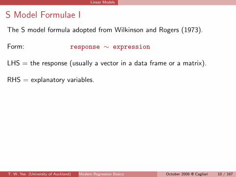
The S model formula adopted from Wilkinson and Rogers (1973).
Form: response ∼ expression
LHS = the response (usually a vector in a data frame or a matrix).
RHS = explanatory variables.
T. W. Yee (University of Auckland) Modern Regression Basics 10/167October 2008 @ Cagliari 10 / 167

Linear Models
S Model Formulae II
Consider
> y ~ x1 + x2 + x3 + f1:f2 + f1 * x1 + f2/f3 + f3:f4:f5 +
+ (f6 + f7)^2
where variables beginning with an x are numeric and those beginning withan f are factors.
By default an intercept is fitted, which is 1. Suppress intercepts by -1.
The interaction f1*f2 is expanded to 1 + f1 + f2 + f1:f2. The termsf1 and f2 are main effects.
A second-order interaction between two factors can be expressed usingfactor:factor: γij . There are other types of interactions. Interactionsbetween a factor and numeric, factor:numeric, produce βjx .
T. W. Yee (University of Auckland) Modern Regression Basics 11/167October 2008 @ Cagliari 11 / 167
Linear Models
S Model Formulae III
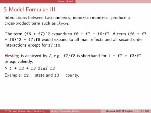
Interactions between two numerics, numeric:numeric, produce across-product term such as βx2x3.
The term (f6 + f7)^2 expands to f6 + f7 + f6:f7. A term (f6 + f7+ f8)^2 - f7:f8 would expand to all main effects and all second-orderinteractions except for f7:f8.
Nesting is achieved by /, e.g., f2/f3 is shorthand for 1 + f2 + f3:f2,or equivalently,
> 1 + f2 + f3 %in% f2
Example: f2 = state and f3 = county.
T. W. Yee (University of Auckland) Modern Regression Basics 12/167October 2008 @ Cagliari 12 / 167

Linear Models
S Model Formulae IV
There are times when you need to use the identity function I(), e.g.,because“^”has special meaning,
> lm(y ~ -1 + offset(a) + x1 + I(x2 - 1) + I(x3^3))
fits
yi = ai + β1xi1 + β2(xi2 − 1) + β3x3i3 + εi ,
εi ∼ iid N(0, σ2), i = 1, . . . , n,
where a is a vector containing the (known) ai .
Other functions: factor(), as.factor(), ordered() terms(),levels(), options().
T. W. Yee (University of Auckland) Modern Regression Basics 13/167October 2008 @ Cagliari 13 / 167

Linear Models
S generics
Generic functions are available for lm objects. They include
add1()
anova()
coef()
deviance()
drop1()
plot()
predict()
print()
residuals()
step()
summary()
update().
Other less used generic functions are alias(), effects(), family(),kappa(), labels(), proj().
Some other functions are model.matrix(), options().
T. W. Yee (University of Auckland) Modern Regression Basics 14/167October 2008 @ Cagliari 14 / 167

Linear Models
The lm() Function
> args(lm)
function (formula, data, subset, weights, na.action, method = "qr",
model = TRUE, x = FALSE, y = FALSE, qr = TRUE, singular.ok = TRUE,
contrasts = NULL, offset, ...)
NULL
The most useful arguments areweights,
subset,
na.action—na.fail(), na.omit(),
contrasts.
Data frames: read.table(), write.table(), na.omit().
T. W. Yee (University of Auckland) Modern Regression Basics 16/167October 2008 @ Cagliari 16 / 167
Linear Models
Factors I
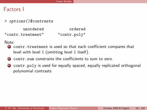
> options()$contrasts
unordered ordered"contr.treatment" "contr.poly"
Note:1 contr.treatment is used so that each coefficient compares that
level with level 1 (omitting level 1 itself).
2 contr.sum constrains the coefficients to sum to zero.
3 contr.poly is used for equally spaced, equally replicated orthogonalpolynomial contrasts
T. W. Yee (University of Auckland) Modern Regression Basics 18/167October 2008 @ Cagliari 18 / 167
Linear Models
Factors II
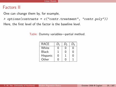
One can change them by, for example,
> options(contrasts = c("contr.treatment", "contr.poly"))
Here, the first level of the factor is the baseline level.
Table: Dummy variables—partial method.
RACE D1 D2 D3
White 0 0 0Black 1 0 0Hispanic 0 1 0Other 0 0 1
T. W. Yee (University of Auckland) Modern Regression Basics 19/167October 2008 @ Cagliari 19 / 167
Linear Models
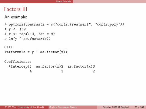
Factors III
An example:
> options(contrasts = c("contr.treatment", "contr.poly"))
> y <- 1:9
> x <- rep(1:3, len = 9)
> lm(y ~ as.factor(x))
Call:lm(formula = y ~ as.factor(x))
Coefficients:(Intercept) as.factor(x)2 as.factor(x)3
4 1 2
T. W. Yee (University of Auckland) Modern Regression Basics 20/167October 2008 @ Cagliari 20 / 167

Linear Models
Factors IV
Another example:
> options(contrasts = c("contr.sum", "contr.poly"))
> lm(y ~ as.factor(x))
Call:lm(formula = y ~ as.factor(x))
Coefficients:(Intercept) as.factor(x)1 as.factor(x)25.000e+00 -1.000e+00 -7.493e-17
T. W. Yee (University of Auckland) Modern Regression Basics 21/167October 2008 @ Cagliari 21 / 167

Linear Models
Topics not done . . .
Other important topics not done:
residual analysis
influential observations
robust regression
variable selection
. . .
T. W. Yee (University of Auckland) Modern Regression Basics 22/167October 2008 @ Cagliari 22 / 167
Generalized Linear Models (GLMs)
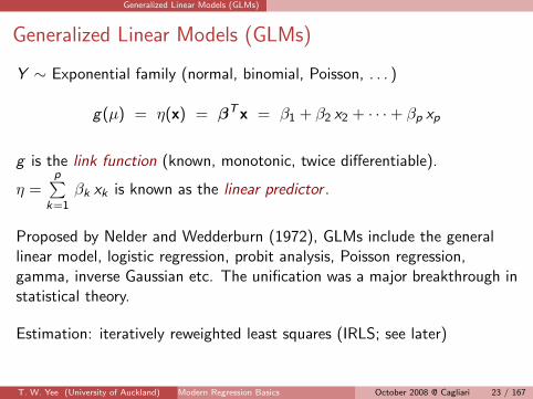
Generalized Linear Models (GLMs)
Y ∼ Exponential family (normal, binomial, Poisson, . . . )
g(µ) = η(x) = βTx = β1 + β2 x2 + · · ·+ βp xp
g is the link function (known, monotonic, twice differentiable).
η =p∑
k=1βk xk is known as the linear predictor .
Proposed by Nelder and Wedderburn (1972), GLMs include the generallinear model, logistic regression, probit analysis, Poisson regression,gamma, inverse Gaussian etc. The unification was a major breakthrough instatistical theory.
Estimation: iteratively reweighted least squares (IRLS; see later)
T. W. Yee (University of Auckland) Modern Regression Basics 23/167October 2008 @ Cagliari 23 / 167
Generalized Linear Models (GLMs)
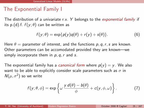
The Exponential Family I
The distribution of a univariate r.v. Y belongs to the exponential family ifits p.(d).f. f (y ; θ) can be written as
f (y ; θ) = exp{p(y)q(θ) + r(y) + s(θ)}. (6)
Here θ = parameter of interest, and the functions p, q, r , s are known.Other parameters can be accomodated provided they are known—wesimply incorporate them in p, q, r and s.
The exponential family has a canonical form where p(y) = y . We alsowant to be able to explicitly consider scale parameters such as σ inN(µ, σ2) so we write
f (y ; θ, φ) = exp
{ω
y d(θ)− b(θ)
φ+ c(y , φ, ω)
}. (7)
T. W. Yee (University of Auckland) Modern Regression Basics 25/167October 2008 @ Cagliari 25 / 167

Generalized Linear Models (GLMs)
The Exponential Family II
Equation (7) belongs to (6) provided φ is known (ω is some knownconstant here). (φ > 0, ω ≥ 0).
θ∗ = d(θ)
is often called the natural parameter of the distribution.
T. W. Yee (University of Auckland) Modern Regression Basics 26/167October 2008 @ Cagliari 26 / 167
Generalized Linear Models (GLMs)
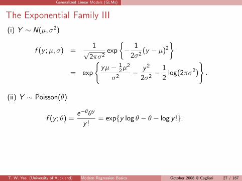
The Exponential Family III
(i) Y ∼ N(µ, σ2)
f (y ;µ, σ) =1√
2πσ2exp
{− 1
2σ2(y − µ)2
}= exp
{yµ− 1
2µ2
σ2− y2
2σ2− 1
2log(2πσ2)
}.
(ii) Y ∼ Poisson(θ)
f (y ; θ) =e−θθy
y != exp{y log θ − θ − log y !}.
T. W. Yee (University of Auckland) Modern Regression Basics 27/167October 2008 @ Cagliari 27 / 167
Generalized Linear Models (GLMs)
The Exponential Family IV
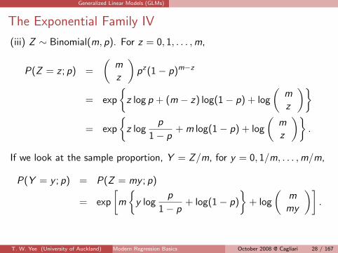
(iii) Z ∼ Binomial(m, p). For z = 0, 1, . . . ,m,
P(Z = z ; p) =
(mz
)pz(1− p)m−z
= exp
{z log p + (m − z) log(1− p) + log
(mz
)}= exp
{z log
p
1− p+ m log(1− p) + log
(mz
)}.
If we look at the sample proportion, Y = Z/m, for y = 0, 1/m, . . . ,m/m,
P(Y = y ; p) = P(Z = my ; p)
= exp
[m
{y log
p
1− p+ log(1− p)
}+ log
(mmy
)].
T. W. Yee (University of Auckland) Modern Regression Basics 28/167October 2008 @ Cagliari 28 / 167
Generalized Linear Models (GLMs)
The Exponential Family V
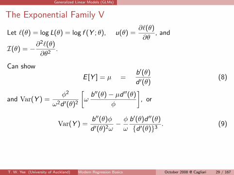
Let `(θ) = log L(θ) = log f (Y ; θ), u(θ) =∂`(θ)
∂θ, and
I(θ) = −∂2`(θ)
∂θ2.
Can show
E [Y ] = µ =b′(θ)
d ′(θ)(8)
and Var(Y ) =φ2
ω2d ′(θ)2
[ω
b′′(θ)− µd ′′(θ)
φ
], or
Var(Y ) =b′′(θ)φ
d ′(θ)2ω− φ
ω
b′(θ)d ′′(θ)
{d ′(θ)}3. (9)
T. W. Yee (University of Auckland) Modern Regression Basics 29/167October 2008 @ Cagliari 29 / 167
Generalized Linear Models (GLMs)
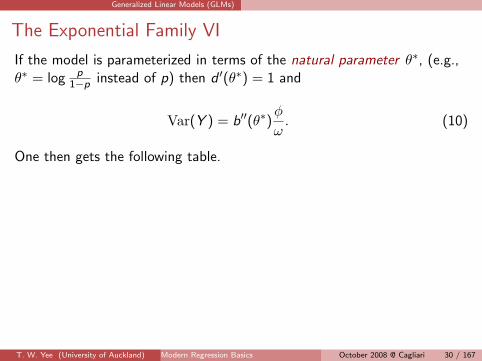
The Exponential Family VI
If the model is parameterized in terms of the natural parameter θ∗, (e.g.,θ∗ = log p
1−p instead of p) then d ′(θ∗) = 1 and
Var(Y ) = b′′(θ∗)φ
ω. (10)
One then gets the following table.
T. W. Yee (University of Auckland) Modern Regression Basics 30/167October 2008 @ Cagliari 30 / 167
Generalized Linear Models (GLMs)
The Exponential Family VII
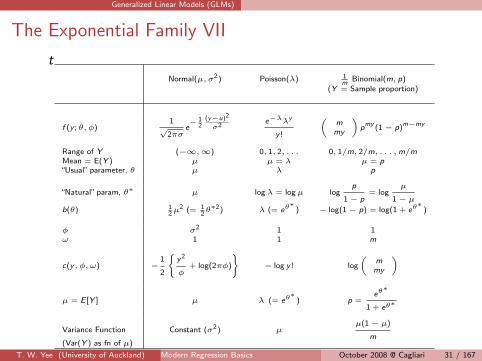
tNormal(µ, σ2) Poisson(λ) 1
mBinomial(m, p)
(Y = Sample proportion)
f (y ; θ, φ)1
√2πσ
e− 1
2(y−u)2
σ2e−λλy
y !
„mmy
«pmy (1− p)m−my
Range of Y (−∞,∞) 0, 1, 2, . . . 0, 1/m, 2/m, . . . , m/mMean = E(Y ) µ µ = λ µ = p“Usual” parameter, θ µ λ p
“Natural” param, θ∗ µ log λ = log µ logp
1− p= log
µ
1− µ
b(θ) 12µ2 (= 1
2θ∗2) λ (= eθ∗ ) − log(1− p) = log(1 + eθ∗ )
φ σ2 1 1ω 1 1 m
c(y, φ, ω) −1
2
(y2
φ+ log(2πφ)
)− log y ! log
„mmy
«
µ = E [Y ] µ λ (= eθ∗ ) p =eθ∗
1 + eθ∗
Variance Function Constant (σ2) µµ(1− µ)
m(Var(Y ) as fn of µ)
T. W. Yee (University of Auckland) Modern Regression Basics 31/167October 2008 @ Cagliari 31 / 167
Generalized Linear Models (GLMs)
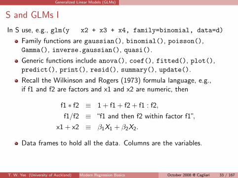
S and GLMs I
In S use, e.g., glm(y x2 + x3 + x4, family=binomial, data=d)
Family functions are gaussian(), binomial(), poisson(),Gamma(), inverse.gaussian(), quasi().
Generic functions include anova(), coef(), fitted(), plot(),predict(), print(), resid(), summary(), update().
Recall the Wilkinson and Rogers (1973) formula language, e.g.,if f1 and f2 are factors and x1 and x2 are numeric, then
f1 ∗ f2 ≡ 1 + f1 + f2 + f1 : f2,
f1/f2 ≡ “f1 and then f2 within factor f1”,
x1 + x2 ≡ β1X1 + β2X2.
Data frames to hold all the data. Columns are the variables.
T. W. Yee (University of Auckland) Modern Regression Basics 33/167October 2008 @ Cagliari 33 / 167
Generalized Linear Models (GLMs)
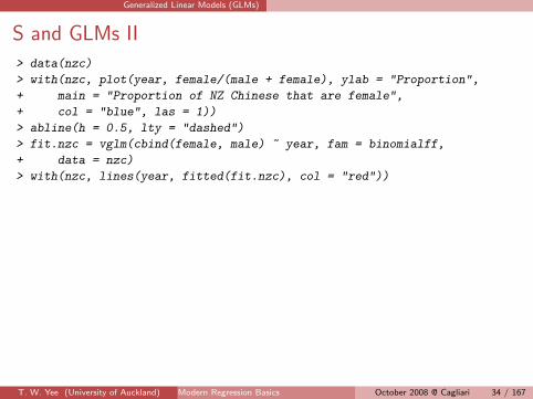
S and GLMs II
> data(nzc)
> with(nzc, plot(year, female/(male + female), ylab = "Proportion",
+ main = "Proportion of NZ Chinese that are female",
+ col = "blue", las = 1))
> abline(h = 0.5, lty = "dashed")
> fit.nzc = vglm(cbind(female, male) ~ year, fam = binomialff,
+ data = nzc)
> with(nzc, lines(year, fitted(fit.nzc), col = "red"))
T. W. Yee (University of Auckland) Modern Regression Basics 34/167October 2008 @ Cagliari 34 / 167

Generalized Linear Models (GLMs)
S and GLMs III
● ● ● ● ● ●● ● ●
●
●
●
●
●
●
●
●●
●
●
●
●●
●● ●
1880 1900 1920 1940 1960 1980 2000
0.0
0.1
0.2
0.3
0.4
0.5
Proportion of NZ Chinese that are female
year
Pro
port
ion
T. W. Yee (University of Auckland) Modern Regression Basics 35/167October 2008 @ Cagliari 35 / 167

Generalized Linear Models (GLMs)
S and GLMs IV
> with(nzc, plot(year, female/(male + female), ylab = "Proportion",
+ main = "Proportion of NZ Chinese that are female",
+ col = "blue", las = 1))
> abline(h = 0.5, lty = "dashed")
> fit.nzc = vglm(cbind(female, male) ~ poly(year,
+ 2), fam = binomialff, data = nzc)
● ● ● ● ● ●● ● ●
●
●
●
●
●
●
●
●●
●
●
●
●●
●● ●
1880 1900 1920 1940 1960 1980 2000
0.0
0.1
0.2
0.3
0.4
0.5
Proportion of NZ Chinese that are female
year
Pro
port
ion
T. W. Yee (University of Auckland) Modern Regression Basics 36/167October 2008 @ Cagliari 36 / 167

Generalized Linear Models (GLMs)
Logistic regression I
> options(contrasts = c("contr.treatment", "contr.poly"))
> y <- cbind(c(5, 20, 15, 10), c(20, 10, 10, 10))
> x <- 1:4
> fit <- glm(y ~ as.factor(x), family = binomial)
> fit
Call: glm(formula = y ~ as.factor(x), family = binomial)
Coefficients:
(Intercept) as.factor(x)2 as.factor(x)3 as.factor(x)4
-1.386 2.079 1.792 1.386
Degrees of Freedom: 3 Total (i.e. Null); 0 Residual
Null Deviance: 14.04
Residual Deviance: 4.441e-15 AIC: 22.14
> exp(coef(fit)[-1])
T. W. Yee (University of Auckland) Modern Regression Basics 38/167October 2008 @ Cagliari 38 / 167
Generalized Linear Models (GLMs)
Logistic regression II
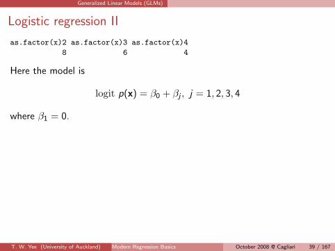
as.factor(x)2 as.factor(x)3 as.factor(x)4
8 6 4
Here the model is
logit p(x) = β0 + βj , j = 1, 2, 3, 4
where β1 = 0.
T. W. Yee (University of Auckland) Modern Regression Basics 39/167October 2008 @ Cagliari 39 / 167
Generalized Linear Models (GLMs)
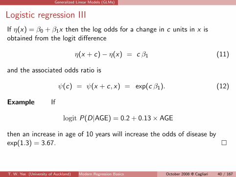
Logistic regression III
If η(x) = β0 + β1x then the log odds for a change in c units in x isobtained from the logit difference
η(x + c)− η(x) = c β1 (11)
and the associated odds ratio is
ψ(c) = ψ(x + c, x) = exp(c β1). (12)
Example If
logit P(D|AGE) = 0.2 + 0.13× AGE
then an increase in age of 10 years will increase the odds of disease byexp(1.3) = 3.67. �
T. W. Yee (University of Auckland) Modern Regression Basics 40/167October 2008 @ Cagliari 40 / 167
Generalized Linear Models (GLMs)
Logistic regression IV
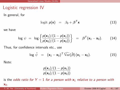
In general, for
logit p(x) = β0 + βTx (13)
we have
log ψ = log
{p(x1)/(1− p(x1))
p(x0)/(1− p(x0))
}= βT (x1 − x0). (14)
Thus, for confidence intervals etc., use
log ψ = (x1 − x0)T Var(β) (x1 − x0). (15)
Note:
p(x1)/(1− p(x1))
p(x0)/(1− p(x0))
is the odds ratio for Y = 1 for a person with x1 relative to a person withx0.T. W. Yee (University of Auckland) Modern Regression Basics 41/167October 2008 @ Cagliari 41 / 167

Generalized Linear Models (GLMs)
Some extensions of GLMs
Quasi-likelihood (Wedderburn, 1974)
Composite link functions (Thompson and Baker, 1981)
IRLS for other models (Green, 1984)
Double Exponential Families (Efron, 1986)
Generalized Estimating Equations (GEE; Liang and Zeger, 1986)
Generalized linear mixed models (GLMMs)
ANOVA Splines (Wahba and co-workers, 1995)
Polychotomous Regression (Kooperberg and co-workers, 1997)
Multivariate GLMs (Fahrmeir and Tutz, 2001)
Heirarchial GLMs (Nelder and Lee, late 1990’s)
Generalized additive models (GAMs; Hastie and Tibshirani, 1986)
Generalized additive mixed models (GAMMs; Lin, 1998)
Vector GLMs and VGAMs (Yee and Wild, 1996)
T. W. Yee (University of Auckland) Modern Regression Basics 42/167October 2008 @ Cagliari 42 / 167
Smoothing
Smoothing
Smoothing is a powerful tool for exploratory data analysis. It allows adata-driven approach rather than model-driven approach. Allows the datato“speak for itself”.
Probably the central idea is localness, i.e., local behaviour versus globalbehaviour of a function.
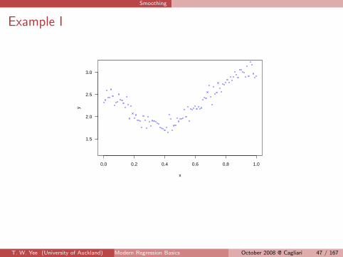
Scatterplot data (xi , yi ), i = 1, . . . , n.
The classical smoothing problem is
yi = f (xi ) + εi , εi ∼ (0, σi ) (16)
independently. Here, f is an arbitary smooth function, and i = 1, . . . , n.
Q: How can f be estimated?
A: If there is no a priori function form for f , one solution is the smoother.T. W. Yee (University of Auckland) Modern Regression Basics 43/167October 2008 @ Cagliari 43 / 167
Smoothing
Uses of Smoothing
Smoothing has many uses, e.g.,
data visualization and EDA
prediction
derivative estimation, e.g., growth curves, acceleration
used as a basis for many modern statistical techniques
T. W. Yee (University of Auckland) Modern Regression Basics 45/167October 2008 @ Cagliari 45 / 167
Smoothing
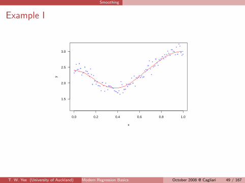
Example I
0.0 0.2 0.4 0.6 0.8 1.0
1.5
2.0
2.5
3.0
x
y
T. W. Yee (University of Auckland) Modern Regression Basics 47/167October 2008 @ Cagliari 47 / 167
Smoothing
Example I
0.0 0.2 0.4 0.6 0.8 1.0
1.5
2.0
2.5
3.0
x
y
T. W. Yee (University of Auckland) Modern Regression Basics 49/167October 2008 @ Cagliari 49 / 167

Smoothing
There are four broad categories of smoothers:
1 series or regression smoothers (polynomials, Fourier regression,regression splines, filtering),
2 Kernel smoothers (N-W, locally weighted averages, local regression,loess),
3 Smoothing splines (roughness penalties),
4 Near neighbour smoothers (running means, medians, Tukeysmoothers).
We will look at kernel smoothers and splines.
T. W. Yee (University of Auckland) Modern Regression Basics 50/167October 2008 @ Cagliari 50 / 167
Smoothing
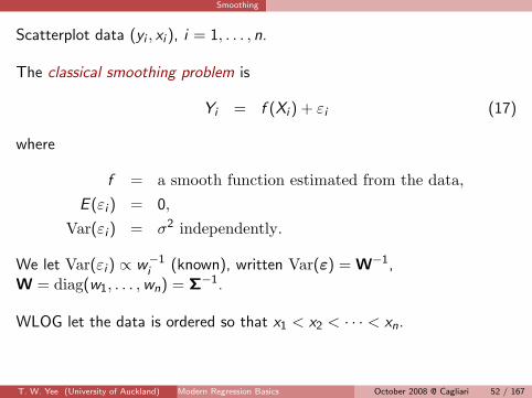
Scatterplot data (yi , xi ), i = 1, . . . , n.
The classical smoothing problem is
Yi = f (Xi ) + εi (17)
where
f = a smooth function estimated from the data,E (εi ) = 0,
Var(εi ) = σ2 independently.
We let Var(εi ) ∝ w−1i (known), written Var(ε) = W−1,
W = diag(w1, . . . ,wn) = Σ−1.
WLOG let the data is ordered so that x1 < x2 < · · · < xn.
T. W. Yee (University of Auckland) Modern Regression Basics 52/167October 2008 @ Cagliari 52 / 167

Smoothing
Kernel Smoothers INadaraya-Watson Estimator
Kernel regression estimators are well-known, easily understood andmathematically tractable.
The Nadaraya-Watson (N-W) estimator estimates f (x) by
fnw (x) =
n∑i=1
K
(x − xi
h
)yi
n∑i=1
K
(x − xi
h
) =
n∑i=1
Kh(x − xi ) yi
n∑i=1
Kh(x − xi )
(18)
where
Kh(u) = h−1K(u
h
). (19)
T. W. Yee (University of Auckland) Modern Regression Basics 54/167October 2008 @ Cagliari 54 / 167

Smoothing
Kernel Smoothers IINadaraya-Watson Estimator
K , a symmetric unimodal function about 0 which integrates to unity,creates the local averaging of values of yi whose corresponding values of xi
are close to the point of estimation x .
The amount of smoothing is controlled by the bandwidth h. Some popularkernel functions are given in Table 2.
As h decreases, the bias decreases and the variance increases.
In practice, the choice of bandwidth h is more crucial than the choice ofkernel function.
T. W. Yee (University of Auckland) Modern Regression Basics 55/167October 2008 @ Cagliari 55 / 167

Smoothing
Kernel Smoothers IIINadaraya-Watson Estimator
0.0 0.2 0.4 0.6 0.8 1.0
1.5
2.0
2.5
3.0
Reg
ress
ion
func
tion
T. W. Yee (University of Auckland) Modern Regression Basics 56/167October 2008 @ Cagliari 56 / 167

Smoothing
Kernel Smoothers IVNadaraya-Watson Estimator
Table: Popular kernel functions. Nb. the quartic is also known as the biweight.
Kernel K (u)
Uniform 12 I (|u| ≤ 1)
Triangle (1− |u|) I (|u| ≤ 1)Epanechnikov 3
4(1− u2) I (|u| ≤ 1)Quartic 15
16(1− u2)2 I (|u| ≤ 1)Tricube 70
81(1− |u|3)3 I (|u| ≤ 1)Triweight 35
32(1− u2)3 I (|u| ≤ 1)
Gaussian exp(−12u2)/
√2π
Cosinus π4 cos(πu/2) I (|u| ≤ 1)
T. W. Yee (University of Auckland) Modern Regression Basics 57/167October 2008 @ Cagliari 57 / 167

Smoothing
Local Regression I
Theoretically elegant and also called local polynomial kernel estimators, ithas favourable asymptotic properties and boundary behaviour.
Idea: estimate f (x0) by“locally”fitting a rth degree polynomial to data viaweighted least squares (WLS).
Example: a local linear kernel estimate for
f (xi ) = 2 exp(−x2i /0.3
2) + 3 exp(−(xi − 1)2/0.72) + εi ,
xi = (i − 1)/n,
εi ∼ N(0, σ = 0.115) independently.
T. W. Yee (University of Auckland) Modern Regression Basics 59/167October 2008 @ Cagliari 59 / 167
Smoothing
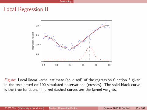
Local Regression II
0.0 0.2 0.4 0.6 0.8 1.0
1.5
2.0
2.5
3.0
Reg
ress
ion
func
tion
Figure: Local linear kernel estimate (solid red) of the regression function f givenin the text based on 100 simulated observations (crosses). The solid black curveis the true function. The red dashed curves are the kernel weights.
T. W. Yee (University of Auckland) Modern Regression Basics 60/167October 2008 @ Cagliari 60 / 167
Smoothing
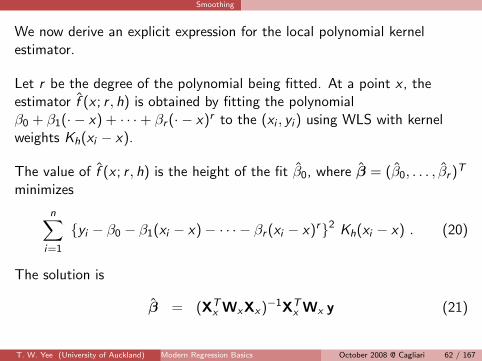
We now derive an explicit expression for the local polynomial kernelestimator.
Let r be the degree of the polynomial being fitted. At a point x , theestimator f (x ; r , h) is obtained by fitting the polynomialβ0 + β1(· − x) + · · ·+ βr (· − x)r to the (xi , yi ) using WLS with kernelweights Kh(xi − x).
The value of f (x ; r , h) is the height of the fit β0, where β = (β0, . . . , βr )T
minimizes
n∑i=1
{yi − β0 − β1(xi − x)− · · · − βr (xi − x)r}2 Kh(xi − x) . (20)
The solution is
β = (XTx WxXx)
−1XTx Wx y (21)
T. W. Yee (University of Auckland) Modern Regression Basics 62/167October 2008 @ Cagliari 62 / 167

Smoothing
where y = (y1, . . . , yn)T ,
Xx =
1 (x1 − x) . . . (x1 − x)r
......
...1 (xn − x) . . . (xn − x)r
is n × (r + 1), and Wx=Diag(Kh(x1 − x), . . . ,Kh(xn − x)). Since theestimator of f (x) is the intercept, we have
f (x ; r , h) = eT1 (XT
x WxXx)−1XT
x Wx y . (22)
T. W. Yee (University of Auckland) Modern Regression Basics 63/167October 2008 @ Cagliari 63 / 167

Smoothing
Simple explicit formulae exist for the N-W estimator (r = 0):
f (x ; 0, h) =
n∑i=1
Kh(xi − x) yi
n∑i=1
Kh(xi − x)
(23)
and the local linear estimator (r = 1):
f (x ; 1, h) = n−1n∑
i=1
{s2(x ; h)− s1(x ; h)(xi − x)} Kh(xi − x) yi
s2(x ; h)s0(x ; h)− s1(x ; h)2(24)
where
sr (x ; h) = n−1n∑
i=1
(xi − x)r Kh(xi − x) . (25)
T. W. Yee (University of Auckland) Modern Regression Basics 65/167October 2008 @ Cagliari 65 / 167
Smoothing
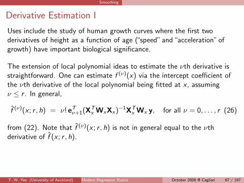
Derivative Estimation I
Uses include the study of human growth curves where the first twoderivatives of height as a function of age (“speed”and“acceleration”ofgrowth) have important biological significance.
The extension of local polynomial ideas to estimate the νth derivative isstraightforward. One can estimate f (ν)(x) via the intercept coefficient ofthe νth derivative of the local polynomial being fitted at x , assumingν ≤ r . In general,
f (ν)(x ; r , h) = ν! eTν+1(X
Tx WxXx)
−1XTx Wx y, for all ν = 0, . . . , r (26)
from (22). Note that f (ν)(x ; r , h) is not in general equal to the νthderivative of f (x ; r , h).
T. W. Yee (University of Auckland) Modern Regression Basics 67/167October 2008 @ Cagliari 67 / 167

Smoothing
Derivative Estimation II
Choosing rIn the early 1990’s Fan and co-workers showed that, for estimating f (ν)(x),there is no increase in variability when passing from an even (i.e., r − νeven) r = ν + 2q order fit to an odd r = ν + 2q + 1 order fit, but whenpassing from an odd r = ν + 2q + 1 order fit to the consecutive evenr = ν + 2q + 2 order there is a price to be paid in terms of increasedvariability. Therefore, even order fits r = ν + 2q are not recommended.Fan and Gijbels (1996) recommend using the lowest odd order, i.e.,r = ν + 1, or occasionally r = ν + 3.
For f choose r = 1 (maybe 3) . . .
For f ′ choose r = 2 (maybe 4) . . .
T. W. Yee (University of Auckland) Modern Regression Basics 68/167October 2008 @ Cagliari 68 / 167

Smoothing
Lowess and Loess I
A popular method based on local regression is Lowess (Cleveland, 1979)and Loess (Cleveland and Devlin, 1988).
Lowess = locally weighted scatterplot smoother, and it robustifies thelocally WLS method above.
The basic idea is to fit a polynomial of degree r locally via (20) and obtainthe fitted values. Then calculate the residuals and assign weights to eachresidual: large/small residuals receive small/large weights respectively.Then perform another local polynomial fit of order r with weights given bythe product of the initial weight and new weight. Thus observationsshowing large residuals at the initial fit are downweighted in the second fit.The above process is repeated a number of times.
Cleveland (1979) recommended r = 1 and 3 iterations (default).
T. W. Yee (University of Auckland) Modern Regression Basics 70/167October 2008 @ Cagliari 70 / 167
Smoothing
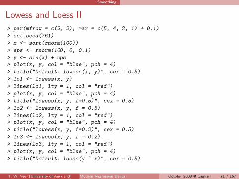
Lowess and Loess II
> par(mfrow = c(2, 2), mar = c(5, 4, 2, 1) + 0.1)
> set.seed(761)
> x <- sort(rnorm(100))
> eps <- rnorm(100, 0, 0.1)
> y <- sin(x) + eps
> plot(x, y, col = "blue", pch = 4)
> title("Default: lowess(x, y)", cex = 0.5)
> lo1 <- lowess(x, y)
> lines(lo1, lty = 1, col = "red")
> plot(x, y, col = "blue", pch = 4)
> title("lowess(x, y, f=0.5)", cex = 0.5)
> lo2 <- lowess(x, y, f = 0.5)
> lines(lo2, lty = 1, col = "red")
> plot(x, y, col = "blue", pch = 4)
> title("lowess(x, y, f=0.2)", cex = 0.5)
> lo3 <- lowess(x, y, f = 0.2)
> lines(lo3, lty = 1, col = "red")
> plot(x, y, col = "blue", pch = 4)
> title("Default: loess(y ~ x)", cex = 0.5)
T. W. Yee (University of Auckland) Modern Regression Basics 71/167October 2008 @ Cagliari 71 / 167
Smoothing
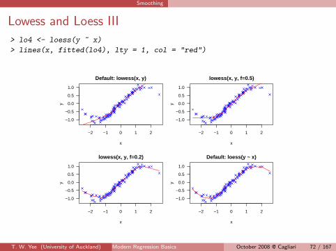
Lowess and Loess III
> lo4 <- loess(y ~ x)
> lines(x, fitted(lo4), lty = 1, col = "red")
−2 −1 0 1 2
−1.0
−0.5
0.0
0.5
1.0
x
y
Default: lowess(x, y)
−2 −1 0 1 2
−1.0
−0.5
0.0
0.5
1.0
x
y
lowess(x, y, f=0.5)
−2 −1 0 1 2
−1.0
−0.5
0.0
0.5
1.0
x
y
lowess(x, y, f=0.2)
−2 −1 0 1 2
−1.0
−0.5
0.0
0.5
1.0
x
y
Default: loess(y ~ x)
T. W. Yee (University of Auckland) Modern Regression Basics 72/167October 2008 @ Cagliari 72 / 167

Smoothing
Lowess and Loess IV
Once again choosing a good bandwidth is crucial.
T. W. Yee (University of Auckland) Modern Regression Basics 73/167October 2008 @ Cagliari 73 / 167

Smoothing
Local Likelihood I
Local likelihood replaces the local least squares criterion by an appropriatelocal log-likelihood criterion.
Example: for binary data (xi , yi ), i = 1, . . . , n, yi = 0 or 1, the locallog-likelihood is
n∑i=1
K
(|xi − x |
h
){yi log pi + (1− yi ) log (1− pi )} (27)
where pi = p(xi ) = P(Y = 1|xi ).
We could model p(x) directly using local polynomials, however, it isusually preferable to use θ(x) = logit p(x). We approximate θ(x) locallyby a polynomial, then choose the polynomial coefficients to maximize thelikelihood.
T. W. Yee (University of Auckland) Modern Regression Basics 75/167October 2008 @ Cagliari 75 / 167

Smoothing
Local Likelihood II
Local likelihood can also be applied to other regression models and densityestimation.
Local likelihood developed by Tibshirani (1984). A good book on the topicis Loader (1999).
T. W. Yee (University of Auckland) Modern Regression Basics 76/167October 2008 @ Cagliari 76 / 167

Smoothing
Regression Splines I
Idea: fit a higher degree polynomial (polynomial regression.)
Some drawbacks:
Polynomials aren’t very local but have a global nature. So usually arenot ok at the boundaries, especially if the degree of the polynomial ishigh [cf. Stone-Weierstrass Theorem];
Individual observations can have a large influence on remote parts ofthe curve;
The polynomial degree cannot be controlled continuously.
Polynomial regression can be fitted using the poly() function, e.g.,
> fit <- lm(y ~ poly(x, 5))
fits a 5th degree polynomial.
T. W. Yee (University of Auckland) Modern Regression Basics 78/167October 2008 @ Cagliari 78 / 167
Smoothing
Regression Splines II
Regression splines use a piecewise polynomial. The regions are separatedby knots (or breakpoints). The positions where each pair of segments joinare called joints. The more knots, the more flexible the family of curvesbecome.
It is customary to force the piecewise polynomials to join smoothly atthese knots. A popular choice are piecewise cubic polynomials withcontinuous 0th, 1st and 2nd derivatives called cubic splines. Using splinesof degree > 3 seldom yields any advantage.
Given a set of knots, the smooth is computed by multiple regression on aset of basis vectors.
T. W. Yee (University of Auckland) Modern Regression Basics 79/167October 2008 @ Cagliari 79 / 167
Smoothing
Regression Splines III
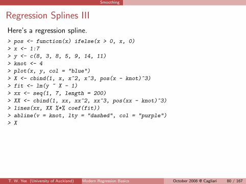
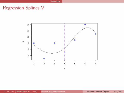
Here’s a regression spline.
> pos <- function(x) ifelse(x > 0, x, 0)
> x <- 1:7
> y <- c(8, 3, 8, 5, 9, 14, 11)
> knot <- 4
> plot(x, y, col = "blue")
> X <- cbind(1, x, x^2, x^3, pos(x - knot)^3)
> fit <- lm(y ~ X - 1)
> xx <- seq(1, 7, length = 200)
> XX <- cbind(1, xx, xx^2, xx^3, pos(xx - knot)^3)
> lines(xx, XX %*% coef(fit))
> abline(v = knot, lty = "dashed", col = "purple")
> X
T. W. Yee (University of Auckland) Modern Regression Basics 80/167October 2008 @ Cagliari 80 / 167
Smoothing
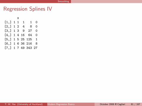
Regression Splines IV
x
[1,] 1 1 1 1 0
[2,] 1 2 4 8 0
[3,] 1 3 9 27 0
[4,] 1 4 16 64 0
[5,] 1 5 25 125 1
[6,] 1 6 36 216 8
[7,] 1 7 49 343 27
T. W. Yee (University of Auckland) Modern Regression Basics 81/167October 2008 @ Cagliari 81 / 167
Smoothing
Regression Splines V
●
●
●
●
●
●
●
1 2 3 4 5 6 7
4
6
8
10
12
14
x
y
T. W. Yee (University of Auckland) Modern Regression Basics 82/167October 2008 @ Cagliari 82 / 167

Smoothing
Regression Splines VI
Definitions: A function f ∈ C k [a, b] if derivatives f ′, f ′′, . . . , f (k) all existand are continuous in [a, b], e.g., |x | /∈ C 1[a, b].Notes:
1 f ∈ C k [a, b] =⇒ f ∈ C k−1[a, b].
2 C [a, b] ≡ C 0[a, b] = {f (t) : f (t) continuous and real valued,a ≤ t ≤ b}.
There are at least two bases for cubic splines:
1 truncated power series easier to understand but is not used inpractice,
2 B-splines harder to understand but is used in practice.
T. W. Yee (University of Auckland) Modern Regression Basics 83/167October 2008 @ Cagliari 83 / 167

Smoothing
Regression Splines VII
Advantages of regression splines:
computationally and statistically simple,
standard parametric inferences are available. For example, testingwhether a knot can be removed and the same polynomial equationused to explain two adjacent segments can be tested by H0 : θj = 0,which is one of the t-tests statistics always printed by a regressionprogram.
Disadvantages of regression splines:
difficult to choose the number of knots,
difficult to choose the position of the knots,
the smoothness of the estimate cannot be varied continuously as afunction of a single smoothing parameter.
T. W. Yee (University of Auckland) Modern Regression Basics 84/167October 2008 @ Cagliari 84 / 167

Smoothing
Regression Splines VIII
Here is a more formal definition of a spline.
In mathematics, a ‘spline’ denotes a function s(x) which is essentially apiecewise polynomial over an interval (a, b), such that a certain number ofits derivatives are continuous for all points in (a, b). More precisely, s(x) isa spline of degree r (some given positive integer) with knots ξ1, . . . , ξK(such that a < ξ1 < ξ2 < · · · < ξK < b) if it satisfies the followingproperties:
for any subinterval (ξj , ξj+1), s(x) is a polynomial of degree r ;(order r + 1);
s ′(x), . . . , s(r−1)(x) are continuous (derivatives), i.e., s ∈ C r−1(a, b);
the rth derivative of s(x) is a step function with jumps at ξ1, . . . , ξK .
Often r is chosen to be 3, and the term cubic spline is then used for theassociated curve.
T. W. Yee (University of Auckland) Modern Regression Basics 85/167October 2008 @ Cagliari 85 / 167

Smoothing
Regression Splines IX
Wold (1974), in a paper reflecting a lot of experience fitting regressionsplines, made the following recommendations when using cubic splines:
1 Knot points should be located at data points,
2 Have as few knots as possible, ensuring that a minimum of 4 or 5observations should fall between knot points,
3 No more than one extremum point and one inflexion point should fallbetween knots (because a cubic is not possible of approximating morevariations),
4 Extrema should be centered in intervals and inflexion points should belocated near knot points.
T. W. Yee (University of Auckland) Modern Regression Basics 86/167October 2008 @ Cagliari 86 / 167
Smoothing
B-Splines I
B-splines form a numerically stable basis for splines.It is convenient to consider splines of a general order, M say.
1 M = 4: cubic spline.
2 M = 3: quadratic spline which has continuous derivatives up to orderM − 2 = 1 at the knots—this is aka a parabolic spline.
3 M = 2: linear spline which has continuous derivatives up to orderM − 2 = 0 at the knots—i.e., the function is continuous.
Let ξ0 (< ξ1) and ξK+1 (> ξK ) be 2 boundary knots. Define theaugmented knot sequence {τ} such that
τ1 ≤ τ2 ≤ · · · ≤ τM ≤ ξ0;
τj+M = ξj , j = 1, . . . ,K ;
ξK+1 ≤ τK+M+1 ≤ · · · ≤ τK+2M .
T. W. Yee (University of Auckland) Modern Regression Basics 88/167October 2008 @ Cagliari 88 / 167

Smoothing
B-Splines II
The actual values of these additional knots beyond the boundary arearbitrary, and it is customary to make them all the same and equal to ξ0and ξK+1 respectively.
Denote by Bi ,m(x) the ith B-spline basis function of order m for the knotsequence {τ}, m ≤ M. They are defined recursively as follows:
For i = 1, . . . ,K + 2M − 1,
Bi ,1(x) =
{1, τi ≤ x < τi+1,0, otherwise;
(28)
T. W. Yee (University of Auckland) Modern Regression Basics 89/167October 2008 @ Cagliari 89 / 167
Smoothing
B-Splines III
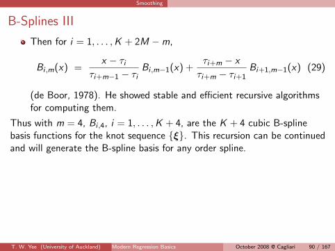
Then for i = 1, . . . ,K + 2M −m,
Bi ,m(x) =x − τi
τi+m−1 − τiBi ,m−1(x) +
τi+m − x
τi+m − τi+1Bi+1,m−1(x) (29)
(de Boor, 1978). He showed stable and efficient recursive algorithmsfor computing them.
Thus with m = 4, Bi ,4, i = 1, . . . ,K + 4, are the K + 4 cubic B-splinebasis functions for the knot sequence {ξ}. This recursion can be continuedand will generate the B-spline basis for any order spline.
T. W. Yee (University of Auckland) Modern Regression Basics 90/167October 2008 @ Cagliari 90 / 167

Smoothing
B-Splines IV
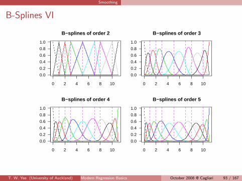
> knots <- c(1:3, 5, 7, 8, 10)
> atx <- seq(0, 11, by = 0.01)
> mycol = (1:(22 + 1))[-7]
> for (ord in 2:5) {
+ B <- bs(x = atx, degree = ord - 1, knots = knots,
+ intercept = TRUE)
+ matplot(atx, B[, 1], type = "l", ylim = 0:1,
+ lty = 2, ylab = "", xlab = "")
+ matlines(atx, B[, -1], col = mycol, lty = 1)
+ title(paste("B-splines of order", ord))
+ abline(v = knots, lty = 2, col = "purple")
+ }
> attr(B, "degree")
[1] 4
> attr(B, "knots")
[1] 1 2 3 5 7 8 10
T. W. Yee (University of Auckland) Modern Regression Basics 91/167October 2008 @ Cagliari 91 / 167

Smoothing
B-Splines V
> attr(B, "Boundary.knots")
[1] 0 11
> attr(B, "intercept")
[1] TRUE
> attr(B, "class")
[1] "bs" "basis"
T. W. Yee (University of Auckland) Modern Regression Basics 92/167October 2008 @ Cagliari 92 / 167
Smoothing
B-Splines VI
0 2 4 6 8 10
0.0
0.2
0.4
0.6
0.8
1.0
B−splines of order 2
0 2 4 6 8 10
0.0
0.2
0.4
0.6
0.8
1.0
B−splines of order 3
0 2 4 6 8 10
0.0
0.2
0.4
0.6
0.8
1.0
B−splines of order 4
0 2 4 6 8 10
0.0
0.2
0.4
0.6
0.8
1.0
B−splines of order 5
T. W. Yee (University of Auckland) Modern Regression Basics 93/167October 2008 @ Cagliari 93 / 167

Smoothing
B-Splines VII
In general, bs() adds ord boundary knots to each end, where theboundary knot values are min(xi ) and max(xi ). If intercept=FALSE thenthe left-most function/column is omitted.
T. W. Yee (University of Auckland) Modern Regression Basics 94/167October 2008 @ Cagliari 94 / 167
Smoothing
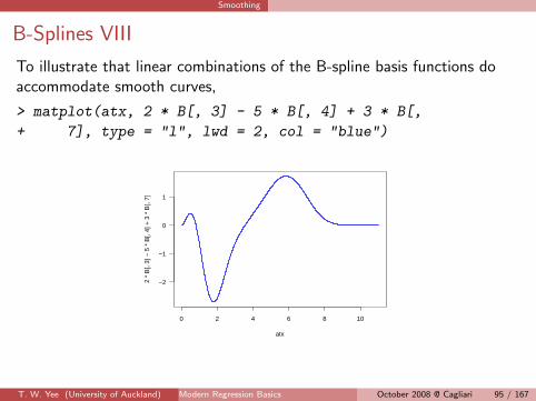
B-Splines VIII
To illustrate that linear combinations of the B-spline basis functions doaccommodate smooth curves,
> matplot(atx, 2 * B[, 3] - 5 * B[, 4] + 3 * B[,
+ 7], type = "l", lwd = 2, col = "blue")
0 2 4 6 8 10
−2
−1
0
1
atx
2 *
B[,
3] −
5 *
B[,
4] +
3 *
B[,
7]
T. W. Yee (University of Auckland) Modern Regression Basics 95/167October 2008 @ Cagliari 95 / 167

Smoothing
B-Splines IX
Here are some additional notes:1 > args(bs)
function (x, df = NULL, knots = NULL, degree = 3, intercept = FALSE,
Boundary.knots = range(x))
NULL
In fact, in Value:, df should be length(knots) + degree +intercept.
2 Safe prediction not as good as smart prediction, e.g., I(bs(x)),poly(scale(x), 2).
T. W. Yee (University of Auckland) Modern Regression Basics 96/167October 2008 @ Cagliari 96 / 167

Smoothing
B-Splines X
3 B-splines are actually defined by means of divided differences. Bi ,m,which is based on knots τi , . . . , τi+m, is defined as
Bi ,m(x) = (τi+m − τi )i+m∑j=i
(x − τj)m−1+
i+m∏s=i ,s 6=j
(τj − τs)
. (30)
Equation (29) follows from this.
T. W. Yee (University of Auckland) Modern Regression Basics 97/167October 2008 @ Cagliari 97 / 167
Smoothing
B-Splines XI
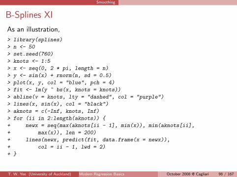
As an illustration,
> library(splines)
> n <- 50
> set.seed(760)
> knots <- 1:5
> x <- seq(0, 2 * pi, length = n)
> y <- sin(x) + rnorm(n, sd = 0.5)
> plot(x, y, col = "blue", pch = 4)
> fit <- lm(y ~ bs(x, knots = knots))
> abline(v = knots, lty = "dashed", col = "purple")
> lines(x, sin(x), col = "black")
> aknots = c(-Inf, knots, Inf)
> for (ii in 2:length(aknots)) {
+ newx = seq(max(aknots[ii - 1], min(x)), min(aknots[ii],
+ max(x)), len = 200)
+ lines(newx, predict(fit, data.frame(x = newx)),
+ col = ii - 1, lwd = 2)
+ }
T. W. Yee (University of Auckland) Modern Regression Basics 98/167October 2008 @ Cagliari 98 / 167
Smoothing
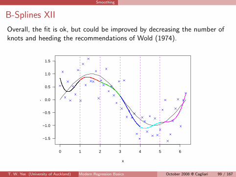
B-Splines XII
Overall, the fit is ok, but could be improved by decreasing the number ofknots and heeding the recommendations of Wold (1974).
0 1 2 3 4 5 6
−1.5
−1.0
−0.5
0.0
0.5
1.0
1.5
x
y
T. W. Yee (University of Auckland) Modern Regression Basics 99/167October 2008 @ Cagliari 99 / 167

Smoothing
B-Splines XIII
Knots with varying multiplicities have an effect illustrated by the following.
●
●●
●
●
●●
●
●
●
●●
●●
●
●●
●
●
●
●
●
●
●
●
●
●
●
●
●●
●
●
●●
●●
●
●
●●
●
●
●
●
●
●
●
●●
0 1 2 3 4 5 6
−1
0
1
2Multiplicity 1
●
●●
●
●
●●
●
●
●
●●
●●
●
●●
●
●
●
●
●
●
●
●
●
●
●
●
●●
●
●
●●
●●
●
●
●●
●
●
●
●
●
●
●
●●
0 1 2 3 4 5 6
−1
0
1
2Multiplicity 2
●
●●
●
●
●●
●
●
●
●●
●●
●
●●
●
●
●
●
●
●
●
●
●
●
●
●
●●
●
●
●●
●●
●
●
●●
●
●
●
●
●
●
●
●●
0 1 2 3 4 5 6
−1
0
1
2Multiplicity 3
●
●●
●
●
●●
●
●
●
●●
●●
●
●●
●
●
●
●
●
●
●
●
●
●
●
●
●●
●
●
●●
●●
●
●
●●
●
●
●
●
●
●
●
●●
0 1 2 3 4 5 6
−1
0
1
2Multiplicity 4
T. W. Yee (University of Auckland) Modern Regression Basics 100/167October 2008 @ Cagliari 100 / 167

Smoothing
Natural Splines I
A cubic spline on [a, b] is a natural cubic splines (NCS) if its 2nd and 3rdderivatives are 0 at a and b (natural boundary conditions).
Natural splines, a restricted form of B-splines, has been implemented bythe function ns(). Given knots ξ1, . . . , ξK , ns() is linear on (−∞, ξ0] and[ξK+1,∞) where ξ0 and ξK+1 are two extra knots.
ns() chooses these to be the minimum and maximum of the xi
respectively. The result is K + 2 parameters.
T. W. Yee (University of Auckland) Modern Regression Basics 102/167October 2008 @ Cagliari 102 / 167

Smoothing
Natural Splines II
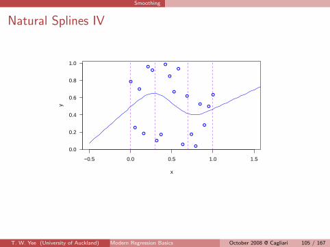
Here’s an example.
> set.seed(21)
> nn = 20
> x = seq(0, 1, len = nn)
> y = runif(nn)
> myknots = c(0.3, 0.7)
> plot(x, y, xlim = c(-0.5, 1.5), col = "blue")
> fit = lm(y ~ ns(x, knot = myknots))
> newx = seq(-0.5, 2.5, len = 100)
> lines(newx, predict(fit, data.frame(x = newx)),
+ col = "blue")
> abline(v = c(range(x), myknots), col = "purple",
+ lty = "dashed")
> coef(fit)
T. W. Yee (University of Auckland) Modern Regression Basics 103/167October 2008 @ Cagliari 103 / 167
Smoothing
Natural Splines III
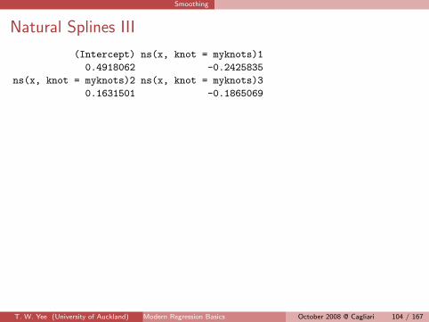
(Intercept) ns(x, knot = myknots)1
0.4918062 -0.2425835
ns(x, knot = myknots)2 ns(x, knot = myknots)3
0.1631501 -0.1865069
T. W. Yee (University of Auckland) Modern Regression Basics 104/167October 2008 @ Cagliari 104 / 167
Smoothing
Natural Splines IV
●
●
●
●
●●
●
●
●
●
●
●
●
●
●
●
●
●
●
●
−0.5 0.0 0.5 1.0 1.5
0.0
0.2
0.4
0.6
0.8
1.0
x
y
T. W. Yee (University of Auckland) Modern Regression Basics 105/167October 2008 @ Cagliari 105 / 167

Smoothing
Smoothing splines I
Cubic smoothing splines minimize
S(f ) =n∑
i=1
(yi − f (xi ))2 + λ
∫ b
a{f ′′(x)}2 dx , (31)
over a Sobolev space of order 2. Here, a < x1 < · · · < xn < b for some aand b, and λ ≥ 0.
The terms of S(f ):
1 The first penalizes lack-of-fit;
2 the second penalizes wiggliness.
These two conflicting quantities are weighted by the non-negativesmoothing parameter λ.
T. W. Yee (University of Auckland) Modern Regression Basics 107/167October 2008 @ Cagliari 107 / 167

Smoothing
Smoothing splines II
Larger values of λ produce more smoother curves.
As λ→∞, f ′′(x) → 0 and the solution is a least squares line.
As λ→ 0, the solution tends to an interpolating twice-differentiablefunction.
(31) fits into the“penalty function”approach (Green and Silverman, 1994).Penalized least squares minimizes
(y − f)T Σ−1(y − f) + fTKf.
Solution:f = A(λ) y
where A(λ) = (In + ΣK)−1 is the influence or smoother matrix .
T. W. Yee (University of Auckland) Modern Regression Basics 108/167October 2008 @ Cagliari 108 / 167
Smoothing
Some notes I
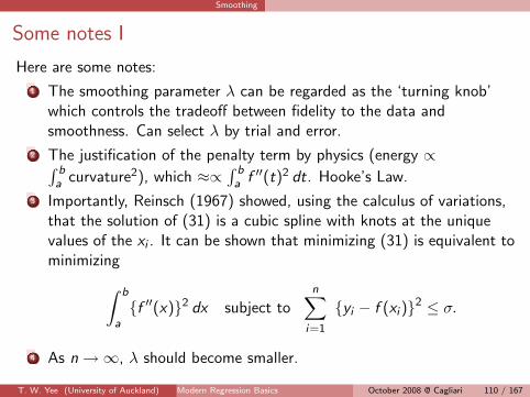
Here are some notes:
1 The smoothing parameter λ can be regarded as the ‘turning knob’which controls the tradeoff between fidelity to the data andsmoothness. Can select λ by trial and error.
2 The justification of the penalty term by physics (energy ∝∫ ba curvature2), which ≈∝
∫ ba f ′′(t)2 dt. Hooke’s Law.
3 Importantly, Reinsch (1967) showed, using the calculus of variations,that the solution of (31) is a cubic spline with knots at the uniquevalues of the xi . It can be shown that minimizing (31) is equivalent tominimizing∫ b
a{f ′′(x)}2 dx subject to
n∑i=1
{yi − f (xi )}2 ≤ σ.
4 As n →∞, λ should become smaller.
T. W. Yee (University of Auckland) Modern Regression Basics 110/167October 2008 @ Cagliari 110 / 167
Smoothing
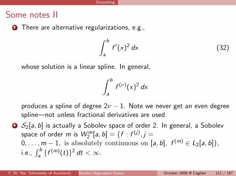
Some notes II5 There are alternative regularizations, e.g.,∫ b
af ′(x)2 dx (32)
whose solution is a linear spline. In general,∫ b
af (ν)(x)2 dx
produces a spline of degree 2ν − 1. Note we never get an even degreespline—not unless fractional derivatives are used.
6 S2[a, b] is actually a Sobolev space of order 2. In general, a Sobolevspace of order m is W m
2 [a, b] = {f : f (j), j =0, . . . ,m − 1, is absolutely continuous on [a, b], f (m) ∈ L2[a, b]},i.e.,
∫ ba {f
(m)(t)}2 dt <∞.
T. W. Yee (University of Auckland) Modern Regression Basics 111/167October 2008 @ Cagliari 111 / 167
Smoothing
Some notes III
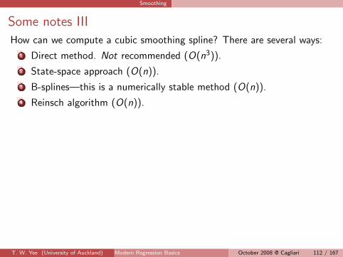
How can we compute a cubic smoothing spline? There are several ways:
1 Direct method. Not recommended (O(n3)).
2 State-space approach (O(n)).
3 B-splines—this is a numerically stable method (O(n)).
4 Reinsch algorithm (O(n)).
T. W. Yee (University of Auckland) Modern Regression Basics 112/167October 2008 @ Cagliari 112 / 167

Smoothing
> args(smooth.spline)
function (x, y = NULL, w = NULL, df, spar = NULL, cv = FALSE,
all.knots = FALSE, nknots = NULL, keep.data = TRUE, df.offset = 0,
penalty = 1, control.spar = list())
NULL
For basic use, use the arguments df.Here’s an example.
> data(cars)
> with(cars, plot(speed, dist, main = "data(cars) & smoothing splines"))
> cars.spl <- with(cars, smooth.spline(speed, dist))
> cars.spl
Call:
smooth.spline(x = speed, y = dist)
Smoothing Parameter spar= 0.7801305 lambda= 0.1112206 (11 iterations)
Equivalent Degrees of Freedom (Df): 2.635278
Penalized Criterion: 4187.776
GCV: 244.1044
T. W. Yee (University of Auckland) Modern Regression Basics 114/167October 2008 @ Cagliari 114 / 167

Smoothing
This example has duplicate points, so avoid cv=TRUE.
> lines(cars.spl, col = "blue")
> with(cars, lines(smooth.spline(speed, dist, df = 10),
+ lty = 2, col = "red", lwd = 2))
> with(cars.spl, legend(5, 120, c(paste("default [C.V.] => df =",
+ round(df, 1)), "s( * , df = 10)"), col = c("blue",
+ "red"), lty = 1:2, lwd = 1:2, bg = "bisque"))
●
●
●
●
●
●
●
●
●
●
●
●
●●● ●
●●
●
●
●
●
●
●
●
●
●
●
●
●
●
●
●
●
●
●
●
●
●
●●●
● ●
●
●
●●
●
●
5 10 15 20 25
0
20
40
60
80
100
120
data(cars) & smoothing splines
speed
dist
default [C.V.] => df = 2.6s( * , df = 10)
T. W. Yee (University of Auckland) Modern Regression Basics 115/167October 2008 @ Cagliari 115 / 167
Smoothing
Smoothing—Some General Theory I
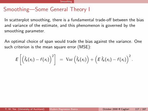
In scatterplot smoothing, there is a fundamental trade-off between the biasand variance of the estimate, and this phenomenon is governed by thesmoothing parameter.
An optimal choice of span would trade the bias against the variance. Onesuch criterion is the mean square error (MSE):
E
[(fk(xi )− f (xi )
)2]
= Var(fk(xi )
)+(E fk(xi )− f (xi )
)2.
T. W. Yee (University of Auckland) Modern Regression Basics 117/167October 2008 @ Cagliari 117 / 167

Smoothing
Linear Smoothers I
A smoother is linear if
S(a y1 + b y2|x) = aS(y1|x) + b S(y2|x) (33)
for any constants a and b. That is,
y = Sy (34)
where S does not depend on y.
S is referred to as the influence (or smoother) matrix .
Examples: For the bin, running-mean, running-line, regression spline,cubic spline, kernel and local polynomial kernel smoothers are all linearsmoothers (with a fixed smoothing parameter).
T. W. Yee (University of Auckland) Modern Regression Basics 119/167October 2008 @ Cagliari 119 / 167
Smoothing
Linear Smoothers II
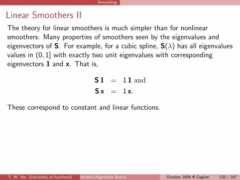
The theory for linear smoothers is much simpler than for nonlinearsmoothers. Many properties of smoothers seen by the eigenvalues andeigenvectors of S. For example, for a cubic spline, S(λ) has all eigenvaluesvalues in (0, 1] with exactly two unit eigenvalues with correspondingeigenvectors 1 and x. That is,
S1 = 1 1 andS x = 1 x.
These correspond to constant and linear functions.
T. W. Yee (University of Auckland) Modern Regression Basics 120/167October 2008 @ Cagliari 120 / 167

Smoothing
Linear Smoothers III● ●
●
●
●
●
●
●
●
●●
●●
●●
●● ● ● ●
1e−05
1e−03
1e−01
Figure: Eigenvalues of a cubic smoothing spline.
T. W. Yee (University of Auckland) Modern Regression Basics 121/167October 2008 @ Cagliari 121 / 167

Smoothing
Degrees of Freedom I
All smoothers allow the user to vary the amount of smoothing done viathe smoothing parameter, e.g., bandwidth, the span, or λ.
However, it would be useful to have some measure of the amount ofsmoothing done. One such measure is the effective degrees of freedom(EDF) of a smooth. It is useful for a number of reasons, e.g., comparingdifferent types of smoothers while keeping the amount of smoothingroughly equal.
The theory of EDF is a natural extension of standard results from thegeneral linear model
Y = Xβ + ε , Var(ε) = σ2 I.
Recall that, if β is p × 1, that
T. W. Yee (University of Auckland) Modern Regression Basics 123/167October 2008 @ Cagliari 123 / 167
Smoothing
Degrees of Freedom II
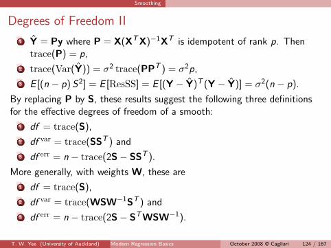
1 Y = Py where P = X(XTX)−1XT is idempotent of rank p. Thentrace(P) = p,
2 trace(Var(Y)) = σ2 trace(PPT ) = σ2p,
3 E [(n − p) S2] = E [ResSS] = E [(Y − Y)T (Y − Y)] = σ2(n − p).
By replacing P by S, these results suggest the following three definitionsfor the effective degrees of freedom of a smooth:
1 df = trace(S),
2 df var = trace(SST ) and
3 df err = n − trace(2S− SST ).
More generally, with weights W, these are
1 df = trace(S),
2 df var = trace(WSW−1ST ) and
3 df err = n − trace(2S− STWSW−1).
T. W. Yee (University of Auckland) Modern Regression Basics 124/167October 2008 @ Cagliari 124 / 167

Smoothing
Degrees of Freedom III
It can be shown that if S is a symmetric projection matrix then trace(S),trace(2S− SST ) and trace(SST ) coincide. For cubic splines, it can beshown that
trace(SST ) ≤ trace(S) ≤ trace(2S− SST )
and that all three of these functions are decreasing in λ.
Notes:
1 df is the most popular and easiest to compute. Cost of df is O(n) formost smoothers.
T. W. Yee (University of Auckland) Modern Regression Basics 125/167October 2008 @ Cagliari 125 / 167

Smoothing
Degrees of Freedom IV
2 2 ≤ the degrees of freedom ≤ the number of distinct xi .Linear fit = 2.The number of distinct xi = interpolant.As the degrees of freedom increases the fit becomes more wiggly. Asmooth with 3 degrees of freedom has approximately the sameflexibility as a quadratic. A value of 4 or 5 degrees of freedom is oftenused as the default value in software, as this can accommodate areasonable amount of nonlinearity without being excessive.
T. W. Yee (University of Auckland) Modern Regression Basics 126/167October 2008 @ Cagliari 126 / 167

Smoothing
Standard Errors I
f = S y =⇒ Var(f) = σ2 SST (35)
Can form pointwise SE bands for f (useful in preventing theover-interpretation of a plot of the estimated function).
But (35) impractical if n is large (all of S needed).
Trick: for cubic splines, Silverman (1985) uses a Bayesian derivation todiscuss the use of the alternative
σ2 S.
Cost is O(n)
T. W. Yee (University of Auckland) Modern Regression Basics 128/167October 2008 @ Cagliari 128 / 167

Smoothing
Equivalent Kernels I
Consider y = Sy for a linear smoother. Plotting the jth row of S versus xi
gives the weights used for the estimate yj . This mimics the kernel functionof a kernel smoother.
The EK for a cubic spline is
κ(u) =1
2exp
(− |u|√
2
)sin
(|u|√
2+π
4
)as n →∞ (Silverman, 1984).
T. W. Yee (University of Auckland) Modern Regression Basics 130/167October 2008 @ Cagliari 130 / 167
Smoothing
Equivalent Kernels II
−5 0 5
0.0
0.1
0.2
0.3
u
EK
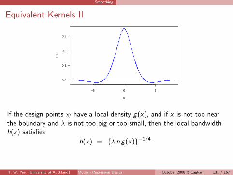
If the design points xi have a local density g(x), and if x is not too nearthe boundary and λ is not too big or too small, then the local bandwidthh(x) satisfies
h(x) = {λ n g(x)}−1/4 .
T. W. Yee (University of Auckland) Modern Regression Basics 131/167October 2008 @ Cagliari 131 / 167
Smoothing
Automatic Smoothing Parameter Selection I
Choosing the bandwidth/smoothing parameter is the most importantdecision for a specified method. We want an automatic way of choosingthe ‘right’ smoothing parameter.
A popular method is cross-validation (CV), and restrict attention to linearsmoothers.
CV idea: leave point (xi , yi ) out one at a time and estimating the smoothat xi based on the remaining n − 1 points.
Choose λCV to minimize the cross-validation sum of squares
CV (λ) =1
n
n∑i=1
{yi − f −i
λ (xi )}2
(36)
T. W. Yee (University of Auckland) Modern Regression Basics 133/167October 2008 @ Cagliari 133 / 167
Smoothing
Automatic Smoothing Parameter Selection II
where f −iλ (xi ) is the fitted value at xi , computed by leaving out the ith
data point.
One can compute (36) naıvely. But there is a trick.
Define f −iλ (xi ) to be the fit obtained by setting the weight of the ith
observation to zero, and increasing the remaining weights so that they sumto unity, i.e.,
f −iλ (xi ) =
n∑j=1j 6=i
sij1− sii
yj . (37)
This means
f −iλ (xi ) =
n∑j=1j 6=i
sij yj + sii f−iλ (xi ) (38)
T. W. Yee (University of Auckland) Modern Regression Basics 134/167October 2008 @ Cagliari 134 / 167

Smoothing
Automatic Smoothing Parameter Selection III
and
yi − f −iλ (xi ) =
yi − fλ(xi )
1− sii. (39)
Thus, CV (λ) can be written
CV (λ) =1
n
n∑i=1
{yi − fλ (xi )
1− sii (λ)
}2
. (40)
So there is no need to compute f −iλ (xi ) naıvely.
In practice, CV sometimes gives questionable performance.
T. W. Yee (University of Auckland) Modern Regression Basics 135/167October 2008 @ Cagliari 135 / 167
Smoothing
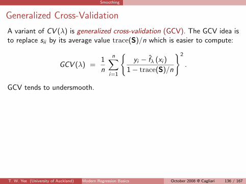
Generalized Cross-Validation
A variant of CV (λ) is generalized cross-validation (GCV). The GCV idea isto replace sii by its average value trace(S)/n which is easier to compute:
GCV (λ) =1
n
n∑i=1
{yi − fλ (xi )
1− trace(S)/n
}2
.
GCV tends to undersmooth.
T. W. Yee (University of Auckland) Modern Regression Basics 136/167October 2008 @ Cagliari 136 / 167

Smoothing
Testing for nonlinearity
Suppose we wish to compare two smooths f1 = S1y and f2 = S2y. Forexample, the smooth f2 might be rougher than f1, and we wish to test if itpicks up any significant bias. A standard case that often arises is when f1is linear, in which case we want to test if the linearity is real. We mustassume that f2 is unbiased, and that f1 is unbiased under H0. LettingResSSj be the residual sum of squares for the jth smooth and γj betrace(2S− STS), then
(ResSS1 − ResSS2)/(γ2 − γ1)
ResSS2/(n − γ1)∼ Fγ2−γ1,n−γ1 (41)
approximately.
T. W. Yee (University of Auckland) Modern Regression Basics 137/167October 2008 @ Cagliari 137 / 167

Smoothing
The Curse of Dimensionality I
Sometimes multidimensional smoothers can work with a moderate numberof inputs. But the curse of dimensionality hinders them in higherdimensions:
local neighbourhoods are empty, or
nearest-neighbourhoods are not local
all points are close to the boundary
sample sizes need to grow exponentially.
T. W. Yee (University of Auckland) Modern Regression Basics 139/167October 2008 @ Cagliari 139 / 167

Smoothing
The Curse of Dimensionality II
That is, neigbourhoods with a fixed number of points become less local asthe dimensions increase. For fixed n, the data becomes more isolated ind-space and smoothers require a larger neighbourhood to find enough datapoints in order to calculate the variance of an estimate. Hence theestimate is no longer local and can be severely biased.
The following illustrates the curse of dimensionality. Suppose we have datauniformly distributed in a d dimensional unit cube. We spread out asubcube from the origin to capture span% of the data. What distance dowe have to reach out on each axis? The next figure gives the answer.Most reasonable high-dimensional procedures assume some structure.
T. W. Yee (University of Auckland) Modern Regression Basics 140/167October 2008 @ Cagliari 140 / 167

Smoothing
The Curse of Dimensionality III
0 20 40 60 80
0.0
0.2
0.4
0.6
0.8
1.0
span (%)
dist
ance
d=1
d=2d=3
d=10
Figure: Distance on each axis of a subcube required to capture span% of the dataof a d dimensional unit cube.
T. W. Yee (University of Auckland) Modern Regression Basics 141/167October 2008 @ Cagliari 141 / 167

Generalized Additive Models (GAMs)
Generalized Additive Models (GAMs) I
For general p, the linear model is
Y = β1X1 + · · ·+ βpXp + ε, ε ∼ N(0, σ2) independently. (42)
This model has some strong assumptions:
1 Linearity, i.e., the effect of each Xk on E (Y ) is linear,
2 Normal errors with zero mean, constant variance, and independent,
3 Additivity, i.e., Xk and X` do not interact; they have an additiveeffect on the response.
T. W. Yee (University of Auckland) Modern Regression Basics 143/167October 2008 @ Cagliari 143 / 167

Generalized Additive Models (GAMs)
Generalized Additive Models (GAMs) II
We relax the linearity assumption.
The linear predictor becomes an additive predictor :
η(x) = f1(x1) + · · ·+ fp(xp), (43)
a sum of arbitary smooth functions.
Additivity is still assumed. Easy to interpret.
Identifiability: the fk(xk) are centred.
Very useful for exploratory data analysis. Allows the data to“speak foritself”.
Some GAM books are Hastie and Tibshirani (1990) and Wood (2006).
T. W. Yee (University of Auckland) Modern Regression Basics 144/167October 2008 @ Cagliari 144 / 167
Generalized Additive Models (GAMs)
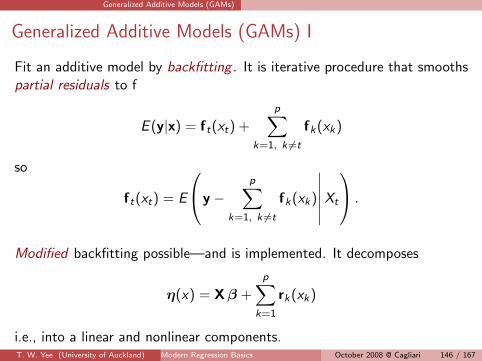
Generalized Additive Models (GAMs) I
Fit an additive model by backfitting . It is iterative procedure that smoothspartial residuals to f
E (y|x) = ft(xt) +
p∑k=1, k 6=t
fk(xk)
so
ft(xt) = E
y −p∑
k=1, k 6=t
fk(xk)
∣∣∣∣∣∣Xt
.
Modified backfitting possible—and is implemented. It decomposes
η(x) = Xβ +
p∑k=1
rk(xk)
i.e., into a linear and nonlinear components.T. W. Yee (University of Auckland) Modern Regression Basics 146/167October 2008 @ Cagliari 146 / 167

Generalized Additive Models (GAMs)
Generalized Additive Models (GAMs) I
Example 1 Kauri data
Y = presence/absence of a tree species, agaaus, which is Agathisaustralis, better known as Kauri, NZ’s most famous tree. Data is from 392sites from the Hunua forest near Auckland.
Figure: Big Kauri tree.
T. W. Yee (University of Auckland) Modern Regression Basics 148/167October 2008 @ Cagliari 148 / 167

Generalized Additive Models (GAMs)
Generalized Additive Models (GAMs) I
174.2 174.6 175.0
−37.4
−37.2
−37.0
−36.8
−36.6
−36.4
Longitude
Latit
ude
●W
H
Figure: The Hunua and Waitakere Ranges.
T. W. Yee (University of Auckland) Modern Regression Basics 150/167October 2008 @ Cagliari 150 / 167

Generalized Additive Models (GAMs)
Generalized Additive Models (GAMs) II
logit P[Yagaaus = 1] = f (altitude)
where f is a smooth function determined from the data.
> data(hunua)
> fit.h = vgam(agaaus ~ s(altitude), binomialff,
+ hunua)
> plot(fit.h, se = TRUE, lcol = "blue", scol = "red",
+ llwd = 2, slwd = 2)
> o = with(hunua, order(altitude))
> with(hunua, plot(altitude[o], fitted(fit.h)[o],
+ type = "l", ylim = 0:1, lwd = 2, col = "blue",
+ xlab = "altitude", ylab = "Fitted value"))
> with(hunua, points(altitude, agaaus + (runif(nrow(hunua)) -
+ 0.5)/30, col = "red"))
T. W. Yee (University of Auckland) Modern Regression Basics 151/167October 2008 @ Cagliari 151 / 167

Generalized Additive Models (GAMs)
Generalized Additive Models (GAMs) III
0 100 200 300 400 500 600
−8
−6
−4
−2
0
2
altitude
s(al
titud
e)
0 100 200 300 400 500 600
0.0
0.2
0.4
0.6
0.8
1.0
altitudeF
itted
val
ue
●●●●●●●
●●
●
●●
●
●
●
●
●
●
●
●
●● ●●
●
● ●
●
●●●
●
●● ●
●●
●●●● ●●● ●●
●●●●
●
● ●●
●
●●●
●
●●●●●●
●●
●●●●●
●
●
●
●● ●●●●●
●
●●
●
●
●
●●
●
●
●
●●●●
●● ●●
●
●
●●
●
●
● ●
●
● ●●
●●
● ●● ●
●
●●
●
● ●●
●
●●
●
● ●●●●● ●●● ●
●
●
● ●
●
●
●●
●
●●●●●
●
●
●●●
●●●●●●
●●●●●
●
●●●●●● ●●●●● ●●●●● ● ●●●●● ● ●●
●●●●●●
●
●●
●
●●●● ●● ●●●●●●● ●●●●●●●● ● ● ●●
●●
●● ●● ●●
●●●
●
●
●●●
●
● ●●● ●● ●
●
● ● ● ●●
●●
●●● ●
●
●
●●
●●
●●
●
●
● ●
●● ●●●
●●
● ●
●
●●
● ● ●● ● ●●●●● ● ● ● ●●●●●
● ●
●● ●●
●●●●●
● ●●●●● ●●●●
●
●●
● ●● ●●●●●
●
●● ● ● ●●● ● ●
●●● ● ●●●
● ●●●●●● ● ●●●
●●●●●●●●●●●●●●●●● ●●●●●
●
Figure: GAM plots of Kauri data in the Hunua ranges.
T. W. Yee (University of Auckland) Modern Regression Basics 152/167October 2008 @ Cagliari 152 / 167
Generalized Additive Models (GAMs)
Generalized Additive Models (GAMs) IV
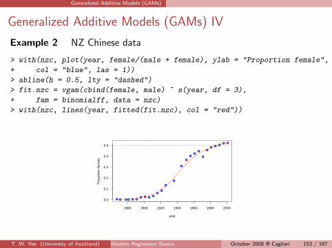
Example 2 NZ Chinese data
> with(nzc, plot(year, female/(male + female), ylab = "Proportion female",
+ col = "blue", las = 1))
> abline(h = 0.5, lty = "dashed")
> fit.nzc = vgam(cbind(female, male) ~ s(year, df = 3),
+ fam = binomialff, data = nzc)
> with(nzc, lines(year, fitted(fit.nzc), col = "red"))
● ● ● ● ● ●● ● ●
●
●
●
●
●
●
●
●●
●
●
●
●●
●● ●
1880 1900 1920 1940 1960 1980 2000
0.0
0.1
0.2
0.3
0.4
0.5
year
Pro
port
ion
fem
ale
T. W. Yee (University of Auckland) Modern Regression Basics 153/167October 2008 @ Cagliari 153 / 167
Generalized Additive Models (GAMs)
GAMs I
There are some packages in R which fit GAMs. These include
gam written by Trevor Hastie, is similar to the S-PLUS version
mgcv by Wood, has an emphasis on smoothing parameter selection
gamlss by Londoners. Limited.
T. W. Yee (University of Auckland) Modern Regression Basics 155/167October 2008 @ Cagliari 155 / 167

Introduction to VGLMs and VGAMs
Introduction to VGLMs and VGAMs I
The VGAM package implements several large classes of regression modelsof which vector generalized linear and additive models (VGLMs/VGAMs)are most commonly used.
The primary key words are
maximum likelihood estimation,
iteratively reweighted least squares (IRLS),
Fisher scoring,
additive models.
Other concepts are
reduced rank regression,
constrained ordination,
vector smoothing.
T. W. Yee (University of Auckland) Modern Regression Basics 157/167October 2008 @ Cagliari 157 / 167

Introduction to VGLMs and VGAMs
Introduction to VGLMs and VGAMs II
Basically, VGLMs model each parameter, transformed if necessary, as alinear combination of the explanatory variables. That is,
gj(θj) = ηj = βTj x (44)
where gj is a parameter link function.
VGAMs extend (44) to
gj(θj) = ηj =
p∑k=1
f(j)k(xk), (45)
i.e., an additive model for each parameter.
T. W. Yee (University of Auckland) Modern Regression Basics 158/167October 2008 @ Cagliari 158 / 167
Introduction to VGLMs and VGAMs
Introduction to VGLMs and VGAMs III
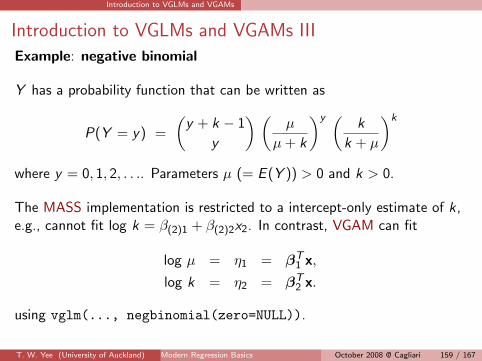
Example: negative binomial
Y has a probability function that can be written as
P(Y = y) =
(y + k − 1
y
) (µ
µ+ k
)y ( k
k + µ
)k
where y = 0, 1, 2, . . .. Parameters µ (= E (Y )) > 0 and k > 0.
The MASS implementation is restricted to a intercept-only estimate of k,e.g., cannot fit log k = β(2)1 + β(2)2x2. In contrast, VGAM can fit
log µ = η1 = βT1 x,
log k = η2 = βT2 x.
using vglm(..., negbinomial(zero=NULL)).
T. W. Yee (University of Auckland) Modern Regression Basics 159/167October 2008 @ Cagliari 159 / 167

Introduction to VGLMs and VGAMs
Introduction to VGLMs and VGAMs IV
Note that it is natural for any positive parameter to have the log link asthe default.
There are also variants of the negative binomial in the VGAM package,e.g., the zero-inflated and zero-altered versions.
T. W. Yee (University of Auckland) Modern Regression Basics 160/167October 2008 @ Cagliari 160 / 167
Introduction to VGLMs and VGAMs
Introduction to VGLMs and VGAMs V
The new framework extends GLMs and GAMs in three main ways:
(i) multivariate responses y and/or linear/additive predictors η arehandled,
(ii) y not restricted to the exponential family,
(iii) ηj need not be a function of a mean µ: ηj = gj(θj) for anyparameter θj .
This formulation is deliberately general so that it encompasses as manydistributions and models as possible. We wish to be limited only by theassumption that the regression coefficients enter through a set of linear oradditive predictors.
Given the covariates, the conditional distribution of the response isintended to be completely general.
T. W. Yee (University of Auckland) Modern Regression Basics 161/167October 2008 @ Cagliari 161 / 167
Introduction to VGLMs and VGAMs
Introduction to VGLMs and VGAMs VI
The scope of VGAM is very broad; it potentially covers
univariate and multivariate distributions,
categorical data analysis,
quantile and expectile regression,
time series,
survival analysis,
mixture models,
extreme value analysis,
nonlinear regression,
. . . .
It conveys GLM/GAM-type modelling to a much broader range of models.
T. W. Yee (University of Auckland) Modern Regression Basics 162/167October 2008 @ Cagliari 162 / 167
Introduction to VGLMs and VGAMs
Introduction to VGLMs and VGAMs VII
LM
RR−VGLM
RR−VLM
VLM
VGLM VGAM
RR−VGAM
QRR−VGLM
VAM
Generalized
Normal errors
Parametric Nonparametric
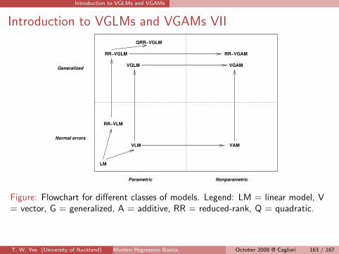
Figure: Flowchart for different classes of models. Legend: LM = linear model, V= vector, G = generalized, A = additive, RR = reduced-rank, Q = quadratic.
T. W. Yee (University of Auckland) Modern Regression Basics 163/167October 2008 @ Cagliari 163 / 167
Introduction to VGLMs and VGAMs
Introduction to VGLMs and VGAMs VIII
tη Model S function Reference
BT1 x1 + BT
2 x2 (= BT x) VGLM vglm() Yee & Hastie (2003)
BT1 x1 +
p1+p2Pk=p1+1
Hk f∗k (xk ) VGAM vgam() Yee & Wild (1996)
BT1 x1 + A ν RR-VGLM rrvglm() Yee & Hastie (2003)
BT1 x1 + A ν +
0BBB@νT D1ν
.
.
.
νT DMν
1CCCA QRR-VGLM cqo() Yee (2004)
BT1 x1 +
RPr=1
fr (νr ) RR-VGAM cao() Yee (2006)
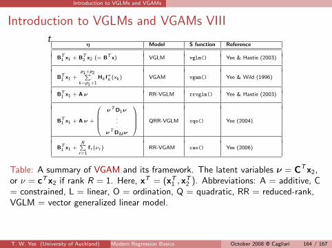
Table: A summary of VGAM and its framework. The latent variables ν = CTx2,or ν = cTx2 if rank R = 1. Here, xT = (xT
1 , xT2 ). Abbreviations: A = additive, C
= constrained, L = linear, O = ordination, Q = quadratic, RR = reduced-rank,VGLM = vector generalized linear model.
T. W. Yee (University of Auckland) Modern Regression Basics 164/167October 2008 @ Cagliari 164 / 167

Concluding Remarks
Concluding Remarks
1 The LM is fundamental and basic to statistical regression modelling.
2 GLMs provide an important unification of several important regressionmodels, e.g., normal, Poisson, binomial, . . . .
3 Smoothing allows the data to“speak for themselves”.
4 GAMs are a very useful data-driven variant of GLMs. Acombinination of GLMs + smoothing. But only c.6 models.
5 VGLMs/VGAMs are GLMs/GAMs but applied to a much wider classof models. We will look at VGLMs/VGAMs in detail later.
T. W. Yee (University of Auckland) Modern Regression Basics 165/167October 2008 @ Cagliari 165 / 167

Concluding Remarks
Finito
T. W. Yee (University of Auckland) Modern Regression Basics 166/167October 2008 @ Cagliari 166 / 167

Concluding Remarks
The End
T. W. Yee (University of Auckland) Modern Regression Basics 167/167October 2008 @ Cagliari 167 / 167