Utah State UniversityDigitalCommons@USU

All Graduate Theses and Dissertations Graduate Studies

5-2008

Models and Algorithms for Addressing Travel TimeVariability: Applications from Optimal PathFinding and Traffic Equilibrium ProblemsZhong ZhouUtah State University

Follow this and additional works at: https://digitalcommons.usu.edu/etd

Part of the Civil Engineering Commons

This Dissertation is brought to you for free and open access by theGraduate Studies at DigitalCommons@USU. It has been accepted forinclusion in All Graduate Theses and Dissertations by an authorizedadministrator of DigitalCommons@USU. For more information, pleasecontact dylan.burns@usu.edu.

Recommended CitationZhou, Zhong, "Models and Algorithms for Addressing Travel Time Variability: Applications from Optimal Path Finding and TrafficEquilibrium Problems" (2008). All Graduate Theses and Dissertations. 129.https://digitalcommons.usu.edu/etd/129

MODELS AND ALGORITHMS FOR ADDRESSING TRAVEL TIME VARIABILITY:

APPLICATIONS FROM OPTIMAL PATH FINDING AND TRAFFIC

EQUILIBRIUM PROBLEMS

by

Zhong Zhou

A dissertation submitted in partial fulfillment of the requirements for the degree

of

DOCTOR OF PHILOSOPHY

in

Civil and Environmental Engineering

Approved: __________________________ ___________________________ Anthony Chen Luis Bastidas Major Professor Committee Member __________________________ ___________________________ Jagath J. Kaluarachchi YangQuan Chen Committee Member Committee Member __________________________ ___________________________ Yong Seog Kim Byron R. Burnham Committee Member Dean of Graduate Studies

UTAH STATE UNIVERSITY Logan, Utah

2008

ii

Copyright © Zhong Zhou 2008 All Right Reserved

iiiABSTRACT

Models and Algorithms for Addressing Travel Time Variability:

Applications from Optimal Path Finding and Traffic Equilibrium Problems

by

Zhong Zhou, Doctor of Philosophy

Utah State University, 2008

Major Professor: Dr. Anthony Chen Department: Civil and Environmental Engineering

An optimal path finding problem and a traffic equilibrium problem are two

important, fundamental, and interrelated topics in the transportation research field. Under

travel time variability, the road networks are considered as stochastic, where the link

travel times are treated as random variables with known probability density functions. By

considering the effect of travel time variability and corresponding risk-taking behavior of

the travelers, this dissertation proposes models and algorithms for addressing travel time

variability with applications from optimal path finding and traffic equilibrium problems.

Specifically, two new optimal path finding models and two novel traffic equilibrium

models are proposed in stochastic networks.

To adaptively determine a reliable path with the minimum travel time budget

required to meet the user-specified reliability threshold α, an adaptive α-reliable path

finding model is proposed. It is formulated as a chance constrained model under a

dynamic programming framework. Then, a discrete-time algorithm is developed based on

ivthe properties of the proposed model. In addition to accounting for the reliability aspect

of travel time variability, the α-reliable mean-excess path finding model further concerns

the unreliability aspect of the late trips beyond the travel time budget. It is formulated as

a stochastic mixed-integer nonlinear program. To solve this difficult problem, a practical

double relaxation procedure is developed.

By recognizing travelers are not only interested in saving their travel time but also

in reducing their risk of being late, a α-reliable mean-excess traffic equilibrium (METE)

model is proposed. Furthermore, a stochastic α-reliable mean-excess traffic equilibrium

(SMETE) model is developed by incorporating the travelers’ perception error, where the

travelers’ route choice decisions are determined by the perceived distribution of the

stochastic travel time. Both models explicitly examine the effects of both reliability and

unreliability aspects of travel time variability in a network equilibrium framework. They

are both formulated as a variational inequality (VI) problem and solved by a route-based

algorithm based on the modified alternating direction method.

In conclusion, this study explores the effects of the various aspects (reliability and

unreliability) of travel time variability on travelers’ route choice decision process by

considering their risk preferences. The proposed models provide novel views of the

optimal path finding problem and the traffic equilibrium problem under an uncertain

environment, and the proposed solution algorithms enable potential applicability for

solving practical problems.

(280 pages)

vACKNOWLEDGMENTS

First of all, I would like to give my appreciation to and sincerely thank my

advisor, Dr. Anthony Chen, for his valuable advice, guidance, and support throughout my

years of graduate study and research at Utah State University. He has dedicated his time

and effort to provide me both supervision and friendship. It has been an honor to learn

from someone of such great expertise and insight and a pleasure to work with someone so

kind and patient. His high standards helped me to achieve work of high quality.

I gratefully acknowledge the other members in my PhD committee, Dr. Luis

Bastidas, Dr. Jagath J. Kaluarachchi, Dr. YangQuan Chen, and Dr. Yong Seog Kim, for

their time, kindness, invaluable comments, and suggestions that improved my research. I

would like to thank all the faculty and staff of the Department of Civil & Environmental

Engineering for their help and intellectual interaction over the years.

All my friends I have at Utah State University—too many to name here—made

my lives at Utah State University happy and enjoyable, and I thank all of them for their

help and friendship.

I would like to express my deepest gratitude to my family for their unconditional

love, understanding, and support throughout my graduate studies. My parents, through

their patience and hard work, sacrificed everything to provide their child a better

education. Athena’s smile and Ziping’s love, understanding, and encouragement made

writing this dissertation an easier task. To them, I dedicate this dissertation.

Zhong Zhou

viCONTENTS

Page

ABSTRACT .................................................................................................................... iii

ACKNOWLEDGMENTS .................................................................................................. v

CONTENTS .................................................................................................................... vi

LIST OF TABLES.............................................................................................................. x

LIST OF FIGURES .......................................................................................................... xii

CHAPTER

1. INTRODUCTION ..................................................................................................... 1

References....................................................................................................... 13

2. LITERATURE REVIEW ........................................................................................ 16

Optimal Path Finding Problems...................................................................... 16 Traffic Equilibrium Problems ......................................................................... 24 The DN-DUE model ........................................................................... 27 The DN-SUE model............................................................................ 30 The SN-DUE model............................................................................ 32 The SN-SUE model ............................................................................ 38 Chapter Summary ........................................................................................... 41 References....................................................................................................... 42 3. ADAPTIVE α-RELIABLE PATH FINDING PROBLEM: FORMULATION AND

SOLUTION ALGORITHM..................................................................................... 54 Abstract ........................................................................................................... 54 Introduction..................................................................................................... 54 The Adaptive α-reliable Path Finding Problem .............................................. 59 Properties of the Adaptive α-reliable Path Finding Problem.......................... 61 Solution Procedure.......................................................................................... 66 Numerical Results........................................................................................... 75 Small network ..................................................................................... 76

vii Large network ..................................................................................... 80 Conclusions..................................................................................................... 85 References....................................................................................................... 86 4. THE α-RELIABLE MEAN-EXCESS PATH FINDING MODEL IN

STOCHASTIC NETWORKS.................................................................................. 89 Abstract ........................................................................................................... 89 Introduction..................................................................................................... 89 The α-reliable Mean-excess Path Finding Model........................................... 95 Notation............................................................................................... 95 Definitions of mean-excess path and its mathematical formulation... 96 Illustrative example........................................................................... 102 Solution Procedure........................................................................................ 105 Numerical Results......................................................................................... 110 Small network ................................................................................... 111 Medium-sized network ..................................................................... 117 Conclusions................................................................................................... 119 References..................................................................................................... 121 5. THE α-RELIABLE MEAN-EXCESS TRAFFIC EQUILIBRIUM MODEL WITH STOCHASTIC TRAVEL TIMES.............................................................. 125 Abstract ......................................................................................................... 125 Introduction................................................................................................... 126 The Mean-Excess Traffic Equilibrium Model.............................................. 134 Notation............................................................................................. 135 Definition of mean-excess travel time .............................................. 137 Illustrative example........................................................................... 141 Equilibrium conditions and variational inequality formulation........ 148 Stochastic travel time under different sources of uncertainty........... 152 Solution Procedure........................................................................................ 158 Numerical Examples..................................................................................... 162 Small network ................................................................................... 162 Medium-size network ....................................................................... 169

viii Conclusions and Future Research................................................................. 172 Reference ...................................................................................................... 174 6. COMPARATIVE ANALYSIS OF THREE USER EQUILIBRIUM MODELS UNDER STOCHASTIC DEMAND .................................................... 180 Abstract ......................................................................................................... 180 Introduction................................................................................................... 181 Models and Formulation ............................................................................... 184 Route choice criteria under an uncertain environment ..................... 184 Path travel time distribution.............................................................. 188 The case of lognormal travel demand distribution ........................... 190 Numerical Results......................................................................................... 194 Comparison of the equilibrium results.............................................. 195 Analysis of the variations of demand level and confidence level..... 199 Conclusions................................................................................................... 203 References..................................................................................................... 204 7. A STOCHASTIC α-RELIABLE MEAN-EXCESS TRAFFIC EQUILIBRIUM MODEL WITH PROBABILISTIC TRAVEL TIMES AND PERCEPTION ERRORS................................................................................................................ 207 Abstract ......................................................................................................... 207 Introduction................................................................................................... 207 Model and Formulation................................................................................. 215 Definition and assumptions............................................................... 215 Route choice criterion under an uncertain environment ................... 220 Perceived mean-excess route travel time.......................................... 223 SMETE conditions and VI formulation............................................ 228 Solution Procedure........................................................................................ 231 Illustrative Examples .................................................................................... 233 Example I .......................................................................................... 234 Example II......................................................................................... 242 Conclusions and Future Research................................................................. 246 References..................................................................................................... 247

ix8. CONCLUSIONS AND RECOMMENDATIONS ................................................ 251 Conclusions................................................................................................... 251 Contributions................................................................................................. 255 Limitations .................................................................................................... 257 Recommendations for Future Research ........................................................ 258 APPENDIX ................................................................................................................. 260 CURRICULUM VITAE................................................................................................. 262

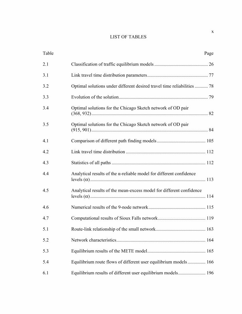
xLIST OF TABLES

Table Page

2.1 Classification of traffic equilibrium models ............................................. 26

3.1 Link travel time distribution parameters................................................... 77

3.2 Optimal solutions under different desired travel time reliabilities ........... 78

3.3 Evolution of the solution........................................................................... 79

3.4 Optimal solutions for the Chicago Sketch network of OD pair (368, 932).................................................................................................. 82 3.5 Optimal solutions for the Chicago Sketch network of OD pair (915, 901).................................................................................................. 84 4.1 Comparison of different path finding models......................................... 105

4.2 Link travel time distribution ................................................................... 112

4.3 Statistics of all paths ............................................................................... 112

4.4 Analytical results of the α-reliable model for different confidence levels (α) ................................................................................................. 113 4.5 Analytical results of the mean-excess model for different confidence

levels (α) ................................................................................................. 114 4.6 Numerical results of the 9-node network................................................ 115

4.7 Computational results of Sioux Falls network........................................ 119

5.1 Route-link relationship of the small network.......................................... 163

5.2 Network characteristics........................................................................... 164

5.3 Equilibrium results of the METE model................................................. 165

5.4 Equilibrium route flows of different user equilibrium models ............... 166

6.1 Equilibrium results of different user equilibrium models....................... 196

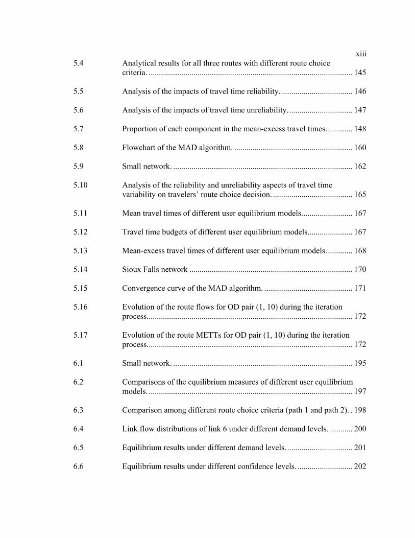
xi7.1 Examine the effects of perception error.................................................. 240

7.2 Route-link relationship of the test network............................................. 243

7.3 Link characteristics ................................................................................. 243

7.4 Route characteristics ............................................................................... 244

xiiLIST OF FIGURES

Figure Page

1.1 Classification of uncertainty (adapted from Haimes, 1998). ...................... 2

1.2 Sources (not exhaustive!) of uncertainty introducing the travel time variability .................................................................................................... 4

2.1 Traffic equilibrium problem and its relations with other surface

transportation applications. ....................................................................... 25 3.1 Flow chart of the discrete-time solution algorithm................................... 70

3.2 Small network. .......................................................................................... 76

3.3 Cumulative distribution curves for two adaptive α-reliable paths. .......... 79

3.4 Optimal paths in the Chicago Sketch network for OD pair (368, 932). ... 81

3.5 Optimal paths in the Chicago Sketch network for OD pair (915, 901). ... 83

4.1 Illustration of the definitions of travel time budget and mean-excess travel time. .............................................................................................. 100 4.2 Hypothetical network used to illustrate the different path finding models. .................................................................................................... 103 4.3 Small network. ........................................................................................ 112

4.4 CPU times and the common logarithm of the differences w.r.t. various sample size at α=80%............................................................................. 116

4.5 Sioux Falls network ................................................................................ 118

5.1 Sources (not exhaustive!) of uncertainty introducing the travel time variability ................................................................................................ 127

5.2 Illustration of the travel time budget and mean-excess travel time. ....... 141

5.3 Hypothetical network used to illustrate the different route choice criteria. .................................................................................................... 142

xiii5.4 Analytical results for all three routes with different route choice criteria. .................................................................................................... 145 5.5 Analysis of the impacts of travel time reliability.................................... 146

5.6 Analysis of the impacts of travel time unreliability................................ 147

5.7 Proportion of each component in the mean-excess travel times............. 148

5.8 Flowchart of the MAD algorithm. .......................................................... 160

5.9 Small network. ........................................................................................ 162

5.10 Analysis of the reliability and unreliability aspects of travel time variability on travelers’ route choice decision. ....................................... 165

5.11 Mean travel times of different user equilibrium models......................... 167

5.12 Travel time budgets of different user equilibrium models...................... 167

5.13 Mean-excess travel times of different user equilibrium models. ............ 168

5.14 Sioux Falls network ................................................................................ 170

5.15 Convergence curve of the MAD algorithm. ........................................... 171

5.16 Evolution of the route flows for OD pair (1, 10) during the iteration process..................................................................................................... 172

5.17 Evolution of the route METTs for OD pair (1, 10) during the iteration

process..................................................................................................... 172 6.1 Small network. ........................................................................................ 195

6.2 Comparisons of the equilibrium measures of different user equilibrium models. .................................................................................................... 197

6.3 Comparison among different route choice criteria (path 1 and path 2). . 198

6.4 Link flow distributions of link 6 under different demand levels. ........... 200

6.5 Equilibrium results under different demand levels. ................................ 201

6.6 Equilibrium results under different confidence levels. ........................... 202

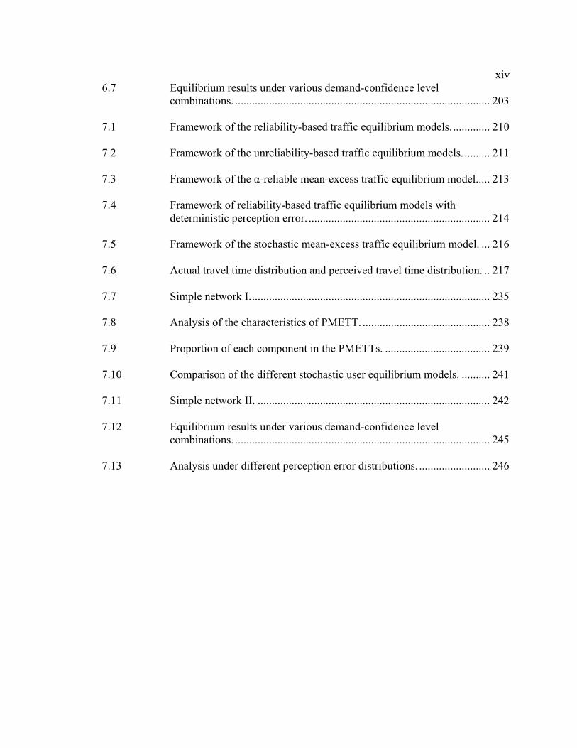
xiv6.7 Equilibrium results under various demand-confidence level combinations. .......................................................................................... 203 7.1 Framework of the reliability-based traffic equilibrium models. ............. 210

7.2 Framework of the unreliability-based traffic equilibrium models. ......... 211

7.3 Framework of the α-reliable mean-excess traffic equilibrium model..... 213

7.4 Framework of reliability-based traffic equilibrium models with deterministic perception error. ................................................................ 214

7.5 Framework of the stochastic mean-excess traffic equilibrium model. ... 216

7.6 Actual travel time distribution and perceived travel time distribution. .. 217

7.7 Simple network I..................................................................................... 235

7.8 Analysis of the characteristics of PMETT. ............................................. 238

7.9 Proportion of each component in the PMETTs. ..................................... 239

7.10 Comparison of the different stochastic user equilibrium models. .......... 241

7.11 Simple network II. .................................................................................. 242

7.12 Equilibrium results under various demand-confidence level combinations. .......................................................................................... 245 7.13 Analysis under different perception error distributions. ......................... 246

CHAPTER 1

INTRODUCTION

Uncertainty is unavoidable in real life. It surrounds all aspects of decision-making

and affects our daily life as well as society. According to Haimes (1998), uncertainty is:

“the inability to determine the true state of affairs of a system.” In general, uncertainty

can be separated into two main categories: objective uncertainties and subjective

uncertainties. The objective uncertainties can arise from stochastic variability while the

subjective uncertainties may account for incomplete knowledge or information. More

specifically, the stochastic variability may occur due to different time, location, or

individual heterogeneity and the limitation of knowledge may induce the uncertainty of

model, parameter or decision (see Figure 1.1). Similarly, as pointed by Bellman and

Zadeh (1970): “Much of the decision-making in the real world takes place in an

environment in which the goals, the constraints and the consequences of possible actions

are not known precisely.” That is, real-life decisions are usually made in a state of

uncertainty. Furthermore, because of the trade-off between getting more accurate

information and reducing the corresponding expense, uncertainty arises from incomplete

information will almost surely be used in the real-life decision-making process.

Therefore, to model, analyze and solve the problems in uncertain environments has been

an important and active research topic in many areas, such as economics, finance and

engineering.

In transportation, uncertainty is a critical and inseparable part of many problems.

For example, the road network is one of the systems that serves the travel demands in

order to connect people engaged in various activities (e.g., work, traveling, shopping,

2

Figure 1.1 Classification of uncertainty (adapted from Haimes, 1998). etc.) at different locations. The uncertainty of network travel times exists in both supply

side (roadway capacity variation) and demand side (travel demand fluctuation). Figure

1.2 provides an illustration of various sources of uncertainty that contribute to travel time

variability.

From the figure, we can observe that several exogenous sources of uncertainty

exist in the supply side. Weather conditions refer to environmental conditions that can

lead to changes in traveler behavior. For example, travelers may lower their speeds or

increase their headways (spacing between vehicles) due to reduced visibility when fog,

rain or snow is present. Traffic incidents, such as car crashes, breakdowns or debris in

lanes, often disrupt the normal flow of traffic. Work zones are construction activities on

the roadways that usually introduce physical changes to the highway environment. The

number or width of lanes may be changed, shoulders may be eliminated, or roadways

may be temporarily closed. Delays caused by work zones have been regarded as one of

the most frustrating conditions that travelers encounter on their trips. Traffic control

3devices, such as signal timing and ramp metering, also contribute to travel time

variability. The uncertainty introduced by these supply-side sources can be referred to as

stochastic link capacity variations, and typically lead to non-recurrent congestion (Chen

et al., 2002; Lo, Luo, and Siu, 2006; Al-Deek and Emam, 2006).

On the other hand, there are several sources of uncertainty that exist in the

demand side. Travel demand fluctuations can be introduced by temporal factors, such as

time of day, day of week or seasonal effects. Special events are a special case of travel

demand fluctuations, where the traffic flow is significantly different from the ‘typical’

pattern in the vicinity of the event. Population characteristics, such as age, car ownership,

and household income, also affect the propensity of travel demand. Traffic information

provided by Advanced Traveler Information Systems (ATIS) can also influence the

travelers’ trip decision, including their departure time, destination, mode, and route

choice, which consequently affect the traffic flow pattern. These demand variations

usually lead to recurrent congestion (Asakura and Kashiwadani, 1991; Clark and

Watling, 2005).

There are also complex interactions between the supply-side and demand-side

sources of uncertainty. For example, bad weather may reduce roadway capacity in the

network, and may at the same time change the spatial and temporal pattern of travel

demand, because travelers may decide to change their departure time, choose a different

route, or even cancel the trip. In short, these uncertain events result in the variation of

traffic flow, which directly contributes to the spatial and temporal variability of network

travel times. Such travel time variability introduces uncertainty for travelers such that

they do not know exactly when they will arrive at the destination. Thus, it is considered

4

Figure 1.2 Sources (not exhaustive!) of uncertainty introducing the travel time variability (modified from van Lint, van Zuylen, and Tu, 2008)

as a risk to a traveler making a trip.

The effects of the travel time variability on travelers’ route choice behaviors have

been studied by several empirical surveys (Abdel-Aty, Kitamura, and Jovanis, 1995;

Small et al., 1999; Lam, 2000; FHWA, 2001; Brownstone et al., 2003; Cambridge

Systematics et al., 2003; Recker et al., 2005). Abdel-Aty, Kitamura, and Jovanis (1995)

found that travel time reliability was either the most or second most important factor for

most commuters. In the study by Small et al. (1999), they found that both individual

travelers and freight carriers were strongly averse to scheduling mismatches. For

example, the individual commuters are willing to pay a premium from $0.17 - $0.26

5per/min of standard deviation in order to avoid congestion and to achieve greater

reliability in travel times. Report generated by FHWA (2001) showed that shippers and

carriers assign a value to increases in travel time, ranging from $25 to almost $200 per

hour, depending on the product carried. From the two value-pricing projects in Southern

California, Lam (2000) and Brownstone et al. (2003) also consistently found that

travelers were willing to pay a substantial amount to reduce variability in travel time.

Another study conducted by Recker et al. (2005) on the freeway system in Orange

County, California observed that: (i) both travel time and travel time variability were

higher in peak hours than non-peak hours; (ii) both travel time and travel time variability

were much higher in winter months than in other seasons; and (iii) travel time and travel

time variability were highly correlated. According to these observations, they suggested

that commuters preferred departing earlier to avoid the possible delays caused by travel

time variability. These empirical studies revealed that travelers considered travel time

variability as a risk in their route choice decisions. They are interested in not only travel

time saving but also the travel time variability reduction to minimize risk. Thus, it is

sufficient to say travel time variability is a significant factor for travelers when making

their route choice decisions under risk or circumstances where they do not know with

certainty about the outcome of their decisions.

Furthermore, a recent empirical study conducted by van Lint, van Zuylen, and Tu

(2008) reveals that the travel time distribution is not only very wide but also heavily

skewed with a long fat tail. For example, it has been shown that about 5% of the

“unlucky drivers” incur almost five times as much delay as the 50% of the “fortunate

drivers” on the densely used freeway corridors in the Netherlands. It has also been found

6that the cost of unexpected delay for trucks is another 50 percent to 250 percent higher

(FHWA, 2001). Therefore, the consequence of these heavily skewed travel times on the

right tail (i.e., the late trips with unacceptable travel times) may be much more serious

than those of modest delays and it has a significant impact on travelers’ route choice

behavior.

The uncertainty of travel time variability discussed above can be considered as

objective uncertainty, which cannot be controlled by the travelers. In additional to the

objective uncertainty, the travelers may also encounter subjective uncertainty during their

route choice decision process. In this study, the subjective uncertainty refers to the

travelers’ perception error of the stochastic travel time. That is, the travelers have to make

their trip decision based on their estimated travel time distribution rather than on the

actual travel time distribution due to the inability of the travelers to accurately estimate

the actual travel time distribution.

As shown in Figure 1.2, various sources of uncertainty introduce either recurrent

or non-recurrent congestion. The congestion threatens the mobility, deteriorates the air

quality and affects the satisfaction of highway users as well as the economy. The Texas

Transportation Institute's 2005 Urban Mobility Report (Schrank and Lomax, 2005)

estimated that the national traffic congestion cost is $63.1 billion in the year of 2003.

Corresponding to the dollar losses is 3.7 billion hours of delay and 2.3 billion gallons of

excess fuel consumed. The growth in road traffic combined with constraints on major

infrastructure investment have led to an increased emphasis on advanced transportation

management and information strategies to meet the growing demands by influencing the

travel patterns of road users. In particular, the Advanced Traveler Information Systems

7(ATIS) that utilize recent information technologies, especially the Internet and wireless

communications, are deeply changing the ways we travel. However, there has been

insufficient emphasis on the basic research in trying to understand how travelers make

their travel decisions in response to this travel information. A better understanding of

route choice and the factors that influence the routes chosen are fundamental in

exploiting such strategies to better utilize network capacity and travel information, such

that congestion could be reduced and the whole system performance could be improved.

In this dissertation, we are interested in the optimal path finding problem and the

traffic equilibrium problem in stochastic networks. These two problems are fundamental

and interrelated in transportation system, and inherently incorporate the travelers’ route

choice behaviors and risk preferences.

The optimal path finding problem is an important and intrinsic research topic in

transportation area. It is to find an optimal path according to certain route choice

criterion. Depending on the assumption of travel time characteristics in the network, the

optimal path finding problem can be classified into two cases: deterministic and the

stochastic. In a deterministic environment, the path finding problem is usually defined as

the Shortest Path (SP) problem in terms of distance, time, cost, or a combination of

deterministic attributes (Bellman, 1958; Dijkstra, 1959; Dantzig, 1960); while in an

uncertain environment, the link/path travel time variations and their associated

probability density functions should be explicitly considered when determining the

optimal path. Most existing methods for dealing with travel time variability are based on

the Expected Value Model (EVM), which is to find the optimal path with the minimum

expected travel time. However, the EVM is unable to account for the travel time

8variability. Therefore, the optimal path found by EVM may be risky, i.e., it has a low

expected travel time, yet has poor reliabilities.

Traffic equilibrium problem, also known as the traffic assignment problem, is to

find the equilibrium flow pattern over a given urban transportation network. It is the last

step of the four-step travel forecasting process (Meyer and Miller, 2001; Ortuzar and

Willumsen, 2001). Given the travel demand between origin-destination (O-D) pairs (i.e.,

travelers), and travel cost function for each link of the transportation network, the traffic

equilibrium problem determines the traffic flow pattern and various performance

measures (e.g., total system travel time, fuel consumption and emission, etc.) of the

network. It stems from the relationship between the link travel time and the link flows, or

equivalent from the interactions between congestion and travel decisions. Therefore, a

route choice model is embedded in the traffic equilibrium model, which represents

individual route choice decisions between various O-D pairs, such that the traffic flow

pattern for the whole transportation network is determined. Congestion is explicitly

considered through the link travel time functions and the interactions with route choice

decisions of the travelers. Given an optimal route choice criterion, if congestion effect is

not taken into account and all travelers are choosing route according to this common

criterion, then the traffic equilibrium problem will degenerate to the optimal path finding

problem, where each traveler will travel based on the optimal path finding results

accordingly. However, the travel time variability is naturally neglected in the

conventional user equilibrium (UE) model, where travelers are all assumed to be risk-

neutral and the route choice decisions are based on the expected travel time.

To account for the travel time variability, one popular measure of travelers’ risk

9preference is the travel time reliability. It is concerned with the probability that a trip

between a given O-D pair could be made successfully within a given time interval or a

specified level-of-service (Asakura and Ksahiwadani, 1991; Asakura, 1996). The reports

issued by the Federal Highway Administration (FHWA, 2006) documented that travelers,

especially commuters, do add a 'buffer time' to their expected travel time to ensure more

frequent on-time arrivals when planning a trip. Travelers are expecting the answer to the

questions that concerns with the travel time reliability, such as “how much time do I need

to allow?” or “how reliable is the trip?” However, in reality, considering only the

reliability aspect may not be adequate to describe travelers’ risk preferences under travel

time variability. It does not address travelers’ concern about the unreliability aspect in

their route choice decisions, such as “how bad should I expect from the worse cases?”,

where trip times longer than they expected would be considered as “unreliable” or

“unacceptable” (Cambridge Systematics et al., 2003). Therefore, it is highly desirable to

consider the unreliability aspect of the travel time variability in travelers’ route choice

decision process, especially when we know that the travel time distribution in real world

is generally asymmetric and highly skew with long fat tail.

Therefore, the primary goal of this research is to study the optimal path finding and

traffic equilibrium problem by considering the travelers’ route choice behaviors and risk

preferences under travel time variability. With this overall goal of the research, the

specific objectives of the dissertation can be defined as follows:

1. To explore the travelers’ concern of the reliability aspect of the uncertain travel time

and its effects in their route choice decision process.

2. To investigate traveler’s route choice decision under consideration of both reliability

10and unreliability aspects of travel time variability.

3. To examine the travelers’ perception error on travel time variability and how this

perception error affects travelers’ route choice decision.

4. To develop new optimal path finding and traffic equilibrium models that incorporate

the travelers’ concerns above (reliability, unreliability and perception error) in their

route choice decisions and risk preferences.

5. To formulate the proposed path finding and traffic equilibrium models, and provide

computational efficient and practical solution procedures.

6. To conduct numerical studies to demonstrate the proposed models and solution

procedures.

This dissertation is comprised of eight chapters in total. This chapter briefly

describes the problem statement, the objectives and scope of the research, as well as the

organization of this dissertation.

Chapter 2 provides a literature review of optimal path finding problems and traffic

equilibrium problems.

Chapter 3 and Chapter 4 contain two papers on the optimal path finding problem

on stochastic networks. Chapter 3 proposes an adaptive α-reliable path finding problem,

where a reliable path is determined adaptively by the minimum travel time budget

according to a predefined travel time reliability threshold. That is, during the traveling

period, travelers are able to dynamically adjust their routing strategy and acquire a more

accurate estimation of their travel time budget. This adaptive approach provides travelers

more flexibility to better arrange their schedule and activities. The adaptive α-reliable

path finding problem is formulated as a chance constrained model (CCM), where the

11reliability based chance constraint is explicitly described under the dynamic

programming framework. A discrete-time algorithm is developed to find the adaptive α-

reliable path. The main contributions of this part of research are formulating such

problem, mathematically proving some properties of the proposed model, and providing

reliable and efficient numerical implementations.

Chapter 4 presents an α-reliable mean-excess path finding problem, where the

mean-excess travel time is proposed and adopted as the route choice criterion. This

optimal path finding criterion accounts for not only the reliability aspect that the traveler

wishes to arrive at his destination within the travel time budget, but also the unreliability

aspect of encountering worst travel times beyond the acceptable travel time budget. The

proposed model is formulated as a stochastic nonlinear mixed-integer programming. To

solve this difficult problem, a double-relaxation scheme is developed to find the α-

reliable mean-excess path. The major contributions of this part of the research are in

formulating the optimal path finding problem by considering both reliability and

unreliability concerns of travelers under travel time variability, and in proposing an

efficient and practical solution algorithm. To our best knowledge, there has been no such

study on the optimal path finding problem addressing the reliability and unreliability

aspects together.

Chapter 5, Chapter 6, and Chapter 7 include three papers on the traffic

equilibrium problem in stochastic networks. Chapter 5 proposes an α-reliable mean-

excess traffic equilibrium (METE) model, where travelers attempt to minimize their

individual mean-excess travel time. In this way, both reliability and unreliability aspects

of travel time variability are explicitly incorporated in the travelers’ route choice decision

12process. It simultaneously addresses both questions of "how much time do I need to

allow?" and "how bad should I expect from the worse cases?" Therefore, travelers' route

choice behavior can be considered in a more accurate and complete manner in a network

equilibrium framework to reflect their risk preferences under an uncertain environment.

The model is formulated as a general variational inequality (VI) problem. Qualitative

properties of the model are also rigorously proved. For solving the proposed model, a

route-based traffic assignment algorithm based on the modified alternating direction

method is adopted. The main contributions in this part of research are modeling,

formulating and solving the traffic equilibrium problem that explicitly considers both

reliability and reliability aspects of the travel time variability in travelers’ route choice

decision process.

Chapter 6 presents a comparative analysis of three user equilibrium models under

travel time variability (i.e., the traditional user equilibrium (UE) model, the demand

driven travel time reliability-based user equilibrium (DRUE) model, and the METE

model), where the travel time variability is induced by the day-to-day travel demand

variation. The major contributions of this part of research are to analytically derive the

link/path travel time distributions and equilibrium conditions from the day-to-day travel

demand variation, and to conduct a comparative analysis of the three user equilibrium

models.

Chapter 7 introduces a stochastic mean-excess traffic equilibrium (SMETE)

model. It addresses the effect of travelers’ perception error on their route choice decision

under travel time variability. In the SMETE model, the travelers are assumed to minimize

their individual perceived mean-excess travel time based on the perceived travel time

13distribution that is composed of both distributions of the random path travel time and the

perception error. It reflects the travelers’ perception of the real travel time distribution

based on his/her individual knowledge about the travel time variability. In general, the

perceived travel time distribution is hard to derive and even has no analytical form at all.

Therefore, a moment analysis approach is adopted to derive the perceived mean-excess

travel time. The proposed model is formulated as a variational inequality (VI) problem,

and solved by a route-based algorithm based on the modified alternating direction

method. Qualitative properties of the model are also rigorously proved. To our best

knowledge, this is the first attempt to integrate the traveler's perception error, travel time

reliability and unreliability into a unified traffic equilibrium framework. The

corresponding SMETE model is completely novel. It provides a more complete manner

for considering travelers' route choice decisions to reflect their risk preferences under an

uncertain environment. The major contributions of this part of research are to define and

formulate such model, provide some qualitative properties of the VI formulation, and

develop a solution procedure with potential applicability for solving practical problems.

Chapter 8 is the conclusion of the dissertation. Findings and contributions of this

dissertation are summarized. Further, recommendations for future research are included

in this chapter.

References

Abdel-Aty, M., R. Kitamura, and P. Jovanis. 1995. Exploring route choice behavior using

geographical information system-based alternative routes and hypothetical travel time information input. Transportation Research Record 1493: 74-80.

14Al-Deek, H., and E B. Emam. 2006. New methodology for estimating reliability in

transportation networks with degraded link capacities. Journal of Intelligent Transportation Systems 10(3): 117-129.

Asakura, Y. 1996. Reliability measures of an origin and destination pair in a deteriorated

road network with variable flows, p. 273-288. Proceedings of the Fourth Meeting of the EURO Working Group on Transportation, University of Newcastle upon Tyne, UK.

Asakura, Y., and M. Kashiwadani. 1991. Road network reliability caused by daily

fluctuation of traffic flow. European Transport, Highways & Planning 19: 73-84. Bellman, R. E. 1958. On a routing problem. Quarterly of Applied Mathematics 16: 87-90. Bellman, R. E., and L. A. Zadeh. 1970. Decision making in a fuzzy environment.

Management Science 17: 141-164. Brownstone, D., A. Ghosh, T. F. Golob, C. Kazimi, and D. V. Amelsfort, 2003. Drivers'

willingness-to-pay to reduce travel time: Evidence from the San Diego I-15 congestion pricing project. Transportation Research Part A 37(4): 373-387.

Cambridge Systematics, Inc., Texas Transportation Institute, University of Washington,

Dowling Associates. 2003. Providing a highway system with reliable travel times. NCHRP Report No. 20-58[3], Transportation Research Board, National Research Council, U.S.A.

Chen, A., Yang, H., Lo, H. K., and Tang, W. H. 2002. Capacity reliability of a road

network: An assessment methodology and numerical results. Transportation Research Part B. 36: 225-252.

Clark, S. D., and D. Watling. 2005. Modeling network travel time reliability under

stochastic demand. Transportation Research Part B 39(2): 119-140. Dantzig, G. B. 1960. On the shortest route through a network. Management Science 6:

187-190. Dijkstra, E. W. 1959. A note on two problems in connection with graphs. Numerical

Mathematics 1: 269-271. FHWA. 2001. Creating a Freight Sector within HERS. White paper prepared for FHWA

by HLB Decision Economics, Inc. FHWA. 2006. Travel time reliability: Making it there on time, all the time. Report No.

70, Federal Highway Administration.

15Haimes, Y. Y. 1998. Risk modeling, assessment and management. John Wiley & Sons,

New York. 744 p. Lam, T. 2000. The effect of variability of travel time on route and time-of-day choice.

Unpublished Ph.D. dissertation. University of California, Irvine. 174 p. Lo, H. K., X. W. Luo, and B. W. Y. Siu. 2006. Degradable transport network: Travel

time budget of travelers with heterogeneous risk aversion. Transportation Research Part B 40: 792-806.

Meyer, M. D., and E. J. Miller. 2001. Urban transportation planning: A decision-oriented

approach, McGraw Hill, New York. 656 p. Ortuzar, J. D., and L. G. Willumsen. 2001. Modelling transport, Wiley, New York. 514 p. Recker, W., Y. Chung, J. Park, L. Wang, A. Chen, Z. Ji, H. Liu, M. Horrocks, and J. S.

Oh. 2005. Considering risk-taking behavior in travel time reliability. Report No. 4110, California Partners for Advanced Transit and Highways.

Schrank, D. L., and T. J. Lomax, 2005. The urban mobility report. Texas Transportation

Institutite. Small, K. A., R. Noland, X. Chu, and D. Lewis, 1999. Valuation of travel-time savings

and predictability in congested conditions for highway user-cost estimation. NCHRP Report No. 431, Transportation Research Board, National Research Council, U.S.A.

van Lint, J. W. C., H. J. van Zuylen, and H. Tu. 2008. Travel time unreliability on

freeways: Why measures based on variance tell only half the story. Transportation Research Part A 42(1): 258-277.

16CHAPTER 2

LITERATURE REVIEW

The primary goal of this research is to study the optimal path finding and traffic

equilibrium problems by considering the travelers’ route choice behaviors and risk

preferences under travel time variability. Therefore, the objective of the literature

review is to provide some understanding of the previous research on the optimal path

finding and traffic equilibrium problems.

Optimal Path Finding Problems

Finding optimal path is an important and intrinsic research topic in various fields,

such as operations research, computer science, telecommunication, etc. In transportation,

the optimal path finding problem, in simplicity, is to find an optimal path in terms of

certain route choice criteria (e.g., distance, time, cost or a combination of different

attributes). In a deterministic environment, where link travel time (or link weight, length,

or cost) is assumed to be deterministic and nonnegative in the network, the optimal path

is usually defined as the shortest path with minimum travel time (weight or cost).

Extensive studies have been done to solve the shortest path (SP) problem and many

efficient algorithms have been developed. To find the shortest path between one node to

all other nodes (i.e. One-to-All), several tree building algorithms has been proposed

(Bellman, 1958; Dijkstra, 1959). In order to get the shortest paths between all nodes at

one time, All-to-All algorithms were developed by Floyd (1962) and Dantzig (1966)

based on matrix manipulations. These algorithms have been widely applied in network

17analysis. In the past several decades, a set of studies were conducted on the deterministic

shortest path finding problem (Nicholson, 1966; Dial, 1969; Dial et al. 1979; Ahuja,

Magnanti, and Orlin, 1993; Glover, Klingman, and Philips, 1985; Goldberg and Radzik,

1993; Ziliaskopoulos and Mahmassani, 1993). Excellent reviews on this topic have been

provided by Dreyfus (1969), Steenbrink (1974), Vliet (1978), and Gallo and Pallottino

(1984). The computational performance of various algorithms have been studied and

improved by Dial (1969), Cherkassky, Boldberg, and Radzik (1996), and Zhan and Noon

(1998).

However, in real life situations, the environment is often uncertain. For

transportation, the uncertainties could arise from various sources, such as demand

fluctuations, incidents, bad weather, and traffic control devices (Cambridge Systematics

et al., 2003). Consequently, link travel times are no longer deterministic and have to be

treated as random variables. Therefore, the associated link travel time probability density

functions should be explicitly incorporated in the travelers’ decision process when

determining the optimal path.

Most existing methods for dealing with travel time uncertainty have focused on

the stochastic shortest path (SSP) problem, which is to find the shortest path with the

minimum expected travel time/cost or maximum utility (Loui, 1960; Mirchandani and

Soroush, 1985; Murthy and Sarkar, 1996; Hall, 1986; Fu and Rilett, 1998; Miller-Hooks

and Mahmassani, 2000; Waller and Ziliaskopoulos, 2002; Dean, 2004; Fan, Kalaba, and

Moore, 2005a). Mirchandani (1976) studies the optimal path finding problem where link

travel time follows two independent states according to the Bernoulli distribution. Loui

(1983) and Eiger, Mirchandani, and Soroush (1985) defined the expected utility of

18random link travel time as the link expected utility and the shortest path as the path with

the maximal path expected utility value. The advantage of these methods are that efficient

shortest path algorithms developed for the deterministic setting (Bellman, 1958; Dijkstra,

1959) can be readily adapted to identify the maximum expected utility path when the

linear or exponential utility functions are adopted. Mirchandani and Soroush (1985)

studied the SSP when the utility function is in the quadratic form. Due to the nonadditive

property of the path utility function, i.e. the path utility is not equal to the summation of

link utility value, the principle of optimality in dynamic programming may not hold and

all feasible paths has to be enumerated in their algorithm. The efficiency of the algorithm

was improved by narrowing down the feasible path set through a pruning scheme by

Murthy and Sarkar (1996). Algorithms for determining the maximum expected value path

was also presented under the general nonlinear and non-increasing utility function (Bard

and Bennett, 1991) and the piecewise linear and concave utility function (Murthy and

Sarkar, 1998). To utilize the recent development of the Advanced Traveler Information

System (ATIS), the temporal dimension was also incorporated into the consideration of

finding optimal path with minimum path time/cost or maximum utility. In this stochastic

and dynamic environment, link travel time distribution is assumed to be a function of

time dimension. Hall (1986) is believed to have conducted the first study investigating

the stochastic and dynamic optimal path finding problem, where the optimal path is the

one with the minimum expected path travel time, and the link travel time is assumed to

be discretely distributed. In order to account for the continuous and independent link

travel time distribution, Fu and Rilett (1998) proposed an approximate method to

estimate the expected path travel time and the path travel time variance. He, Kornhauser,

19and Ran (2002) determined the optimal path with the minimum expected disutility

instead of the expected travel time, where the disutility function is calibrated based on the

path travel time distribution. Excellent reviews and discussions on the time-dependent

stochastic shortest path problems can be found in Miller-Hooks and Mahmassani (2000)

and Dean (2004). Furthermore, Waller and Ziliaskopoulos (2002) and Fan, Kalaba, and

Moore (2005a) extended the stochastic shortest path problems to incorporate the

correlation between random link travel times.

However, setting the expected value as the optimality path index is unable to

account for the travel time variability. According to Asakura and Kashiwadani (1991)

and Asakura (1996), travel time reliability considers the probability that a trip between an

O-D pair can be successfully completed within a certain period of time or at a particular

level-of-service. The minimum expected travel time path could be risky for travelers who

are more concerned about the travel time reliability when finding optimal paths in an

uncertain environment. Recent empirical studies (Abdel-Aty, Kitamura, and Jovani,

1995; Small et al., 1999; Lam, 2000; Brownstone et al., 2003) reveal that the travelers are

interested in not only travel time saving but also the reduction of travel time variability,

and consider travel time variability as a risk in their route choice decision. Therefore,

they may prefer a path with slightly greater expected travel time but with lower

probability of encountering very high travel times.

In order to better account for the risk coming from travel time variability, various

optimal path finding models have been proposed. Loui (1983) mentioned that the optimal

path could be the path with the minimum weighted average of the most pessimistic (the

longest) path travel time realization and the most optimistic (the shortest) path travel time

20realization. Yu and Yang (1998) proposed a Min-Max model to identify a robust path

with the minimal possible longest path travel time. In other words, the path travel time in

the worst scenario of the optimal path is better than that of other paths. Similar approach

under the robust optimization framework was developed by Bertsimas and Sim (2003),

where the link travel time distributions are assumed to be symmetrical, bounded and

independent from each other. Both Min-Max and robust models recommend the optimal

path to be the best alternative in the worst situation. Because of the probability of the

longest travel time occurred could be very low, the Min-Max model may provide overly

conservative solutions in a general situation. Thus, this type of model is particular useful

when the consequence of an extreme case is very significant, such as the hazardous

materials transportation, but may not suitable to explain travelers’ daily commuting

behaviors.

By abstracting the random natures of the travel time into two statistical measures,

i.e. mean and variance, Sivakumar and Batta (1994) defined the optimal path as a path

with the least expected path travel time while the path travel time variance is less than a

predefined threshold value. Sen et al. (2001) presented another Mean-Variance model to

seek a path with a minimal compromise value of expected travel time and travel time

variance. However, the Mean-Variance models only consider the first two moments of

the random travel time, and assume symmetrical or nearly symmetrical path travel time

distribution, which is generally not satisfied in practice.

Recent empirical studies (Cambridge Systematics et al., 2003; FHWA, 2006)

show that the path travel time could be highly skew. Using only the mean and variance

may not be sufficient to capture the characteristics of the path travel time distribution

21accurately. Frank (1969) and Mirchandani (1976) suggested the optimal path should be

the path that maximizes the probability of realizing a travel time less than a predefined

threshold. Sigal, Pritsker, and Solberg (1980) considered optimality as the path that has

the highest probability to be the shortest one. These maximum probability models are

equivalent to finding the most reliable path (Chen and Ji, 2005) which can be regarded as

maximizing the travel time reliability measure. However, the maximum probability

models above require enumerating paths and evaluating multiple integrals, which prohibit

their implementations in real size networks. To address this issue, Fan, Kalaba, and

Moore (2005b) proposed a stochastic on-time arrival (SOTA) problem, which is to

determine the next node to visit from the current location, such that the probability of

arriving at the destination node is maximized. The SOTA problem was formulated using

dynamic programming and solved by the Picard’s method of successive approximation.

Instead of generating an optimal path with the maximum path travel time reliability for a

given travel time budget, the SOTA model is able to provide a portfolio of routing

strategies associated with a range of travel time budgets. To avoid the possible non-

convergence of the successive approximation technique, Nie and Fan (2006) developed

an increasing order of time budget (IOTB) algorithm that runs in a polynomial time.

However, the maximal probability models and the SOTA model require travelers have

sufficient knowledge about the network conditions in order to provide a reasonable path

travel time budget or a sound range of travel time budgets as an input to find either the

most reliable path or a portfolio of routing strategies. If the travel time budget is specified

too large, the maximum reliability of most feasible paths or routing strategies will be

close to 1. On the other hand, the corresponding travel time reliability will be extremely

22low if the travel time budget is specified too low, where the optimal path determined by

the maximal probability models and the optimal routing strategies developed by the

SOTA model may be circuitous (i.e., higher expected travel time) by avoiding the risk of

encountering unacceptable delays (i.e., high risk links).

In view of the limitations of the above models, Chen and Ji (2005) provided an

alternative definition of optimality that allows the travelers to specify a confidence level

α for finding a reliable path with the minimum travel time budget such that the

probability of the path travel time less than or equal to this budget is greater or equal to α.

The advantage of this α-reliable path finding model is that it is able to identify a portfolio

of paths with different levels of reliability to suit the travelers' risk preference towards

travel time variability without the prerequisites mentioned in the above models. The α-

reliable path finding problem was formulated as a chance constrained model and solved

by a simulation-based genetic algorithm (SGA) procedure. However, the α-reliable path

defined and generated above is static (or pre-planned) and the travel time reliability

requirement is only promised at the origin. This may not be suitable for the travelers who

desire a more accurate and flexible control of their time schedule and activities. The α-

reliable path with a pre-planned routing strategy may be inappropriate under the

circumstance where the real-time traffic information can be utilized, which is readily

available from the Advanced Traveler Information Systems (ATIS). Furthermore, the

SGA procedure is a heuristic, where the optimal solution cannot be guaranteed, and is

computationally intensive due to the features of simulation and genetic algorithm. Thus,

its application to real-world networks may be limited. Literature on the general stochastic

optimal control (Bellman and Kalaba, 1965; Bertsekas and Tsitsiklis, 1996) has shown

23that the adaptive strategies may generate different results from a pre-planned optimal

strategy in a stochastic environment. Hall (1986) also showed that adaptive strategies are

more efficient than following a pre-planned optimal path in the dynamic and stochastic

shortest path problem. Therefore, it is interested to construct a model to adaptively

determine a α-reliable path, such that travelers are able to dynamically adjust their

routing strategy during the traveling period and acquire more accurate estimation of their

travel time budget. Furthermore, a formulation of the new model is required and a

practical solution algorithm with guaranteed convergence is needed.

From the travelers' point of view, the α-reliable path finding model provides

travelers the answer to the question that concerns with the reliability aspect, such as “how

much time do I need to allow?” or “how reliable the trip is?”. The reports issued by

FHWA (2006) documented that travelers, especially commuters, do add a 'buffer time' to

their expected travel time to ensure more frequent on-time arrivals when planning a trip.

However, considering only the reliability aspect may not be adequate to describe

travelers’ risk preferences under travel time variability. It does not address travelers’

concern about the unreliability aspect in their path selecting decisions, such as “how bad

should I expect from the worse cases?”, where trip time longer than they expected would

be considered as ‘unreliable’ or ‘unacceptable’ (Cambridge Systematics et al., 2003).

Based on the recent empirical study on the Netherlands freeways (van Lint, van Zuylen,

and Tu, 2008), travel time distributions are not only very wide but also heavily skewed

with long tail. It has a significant impact on travelers facing unacceptable risk (i.e.,

unacceptable travel times). For example, it has been shown that about 5% of the “unlucky

drivers” incur almost five times as much delay as the 50% of the “fortunate drivers” on

24densely used freeway corridors in the Netherlands. Therefore, travel time budget adopted

in the α-reliable path finding model may be an inadequate risk measure, which is unable

to evaluate the impacts of the late trips. In other words, it does not assess the magnitude

of the unacceptable travel times exceeding the travel time budget. Thus, it may introduce

an overwhelmingly high trip time to travelers if it is adopted as a decision criterion for

choosing an optimal path under an uncertain environment. Therefore, a new optimal path

finding model, which can better capture the travelers' risk preferences on both the

reliability and unreliability aspects of travel time variability (i.e., reducing the risk of

encountering unacceptable travel times as well as improving the likelihood of arriving on

time), need to be developed. Moreover, a formulation of this new model and a practical

solution procedure are also desired.

Traffic Equilibrium Problems

Traffic equilibrium problem, also known as traffic assignment problem or user

equilibrium problem, is a critical step of the four-step travel forecasting process (Meyer

and Miller, 2001; Ortuzar and Willumsen, 2001) and is regarded as the foundation of

many surface transportation problems. As shown in Figure 2.1, the traffic equilibrium

problem is closely related with the applications of signal control, ramp metering, and

road pricing in traffic management and control, and with applications of route planning

and guidance in traveler information systems. These applications encompass many of the

surface transportation problems we encounter on a daily basis as transportation

professionals. Given travel demand between origin-destination (O-D) pairs (i.e.,

travelers), and travel time function for each link of the transportation network, the traffic

25

Route ChoiceModel

PerformanceMeasures

TransportationNetworkTravelers

TrafficManagementInformation

III: Traveler InformationSystems

II: Traffic Management andControl

I: Traffic Assignment Problem

Figure 2.1. Traffic equilibrium problem and its relations with other surface transportation applications.

equilibrium problem determines the equilibrium traffic flow pattern and various

performance measures (e.g., total system travel time, vehicle miles of travel, vehicle

hours of travel, fuel consumption and emission, etc.) of the network. Route choice model

is inherently embedded in the traffic equilibrium problem, which represents individual

route choice decisions between various O-D pairs, while congestion is explicitly

considered through the travel time functions. The traffic equilibrium problem stems from

the dependence of the link travel time on the link flows. In other words, it represents the

interactions between congestion and travel decisions, such that traffic flow pattern for the

whole transportation network is predicted. Note that, given the optimal route choice

criterion, if the congestion effect is not taken into account and all travelers are choosing

routes according to the same criterion, then the traffic equilibrium problem will

degenerate to the optimal path finding problem, where each traveler will travel based on

the optimal path finding results respectively.

26In the literature, several traffic equilibrium models have been proposed which

differ in:

1. Characterization of the network travel times (i.e., deterministic or stochastic);

2. Traveler’s knowledge of network travel times (i.e., with or without perception error);

3. Route choice behavior, including: criterion/criteria used in route choice decision

process, route cost structure (i.e., additive or nonadditive), and route choice

preference (e.g., risk averse or risk prone);

According to the classification scheme proposed by Chen and Recker (2001), the

traffic equilibrium problems can be divided into four classes under the presence of

congestion using network uncertainty and perception error shown in Table 2.1.

In each model, the following common assumptions are made:

1. To account for congestion effects, travel time is modeled as an increasing function of

flow of vehicles on the link;

2. Each traveler makes a rational route choice decision based on minimizing some

criteria related to average travel times or some disutility measure based on average

travel times and their variances;

Table 2.1. Classification of traffic equilibrium models

Perception Error? No Yes

No DN-DUE DN-SUE Network Uncertainty? Yes SN-DUE SN-SUE

where DN = Deterministic Network, SN = Stochastic Network

DUE = Deterministic User Equilibrium SUE = Stochastic User Equilibrium

27For comparison and discussion purposes, we define the following utility function

for a given route:

p p pU V ε= + , (2.1)

where pV is the systematic component of the utility of route p; pε is the random error

term of route p; and pU is the total utility of route p.

The DN-DUE model

The conventional traffic equilibrium model belongs to the DN-DUE model, where

the network uncertainty and perception error are ignored. Essentially, this model assumes

that travelers consider only the expected values of network travel times and they are

perfectly aware of these expected travel times on the network. According to the utility

function specified above, this means

p p pV E T tθ θ⎡ ⎤= − = −⎣ ⎦ and 0pε = , (2.2)

where pt is the average travel time of route p, and θ is a positive parameter.

At the equilibrium state, no traveler can improve his travel time by unilaterally

changing routes. In other words, the choices of routes made by all travelers result in a

network flow allocation such that all used routes between every origin-destination pair

have equal average travel times and no unused route has a lower average travel time. This

is exactly the Wardrop’s (1952) first principle, which describes the user equilibrium (UE)

condition. Since travel time variability is not considered in the route choice decision, all

travelers in the DN-DUE model are implicitly assumed to be risk neutral.

Depending on the route cost structure, formulations of the DN-DUE model

28include four approaches, including: mathematical programming (e.g., Beckmann,

McGuire, and Winsten, 1956; Sheffi, 1985), nonlinear complementary problem

(Aashtiani, 1979), variational inequality (e.g., Dafermos, 1980; Nagurney, 1993), and

fixed point (Asmuth, 1978). All four approaches can be used to formulate the additive

traffic equilibrium problem (i.e., path cost structure is simply the sum of the link costs on

that path). The additive assumption allows one to express route cost in terms of the sum

of link costs, and the traffic equilibrium problem can be solved without the need to store

paths (Gabriel and Bernstein, 1997; Lo and Chen, 2000). This is a significant benefit

when one needs to solve large-scale network problems (Boyce, Ralevic-Deki, and Bar-

Gera, 2004) because it enables the application of a number of well-known link-based

algorithms (e.g., Frank-Wolfe algorithm (LeBlanc, Morlok, and Pierskalla, 1975;

Fukushima, 1984; Weintraub, Ortiz, and Gonzalez, 1985; Janson and Gorostiza, 1987;

Lee and Nie, 2001), PARTAN algorithm (LeBlanc, Helgason, and Boyce, 1985; Florian,

Guelat, and Spiess, 1987; Arezki and Van Vliet, 1990), restricted simplicial

decomposition (RSD) algorithm (Hearn, Lawphongpanich and Ventura, 1985), and

origin-based algorithm (Bar-Gera, 2002)). There are also route-based algorithms that

solve the same problem explicitly using route-flow variables, which require storing the

links of each individual route. Solutions resulting from a route-based algorithm provide

both the aggregate link-flow solutions and the individual route-flow solutions that are not

readily available from a link-based algorithm. Route-based solution algorithms for the

additive traffic equilibrium problem include the O-D-based Frank-Wolfe algorithm

(Chen, Jayakrishnan, and Tsai, 2002), disaggregate simplicial decomposition (DSD)

algorithm (Larsson and Patriksson, 1992), gradient projection (GP) algorithm (Bertsekas

29and Gafni, 1982; Jayakrishnan et al., 1994), and conjugate gradient projection algorithm

(Lee, Nie, and Chen, 2003). For a comprehensive review and computational study of the

route- and link-based solution algorithms for the additive traffic equilibrium problem, the

readers are referred to Chen, Lee, and Jayakrishnan (2002), and Lee et al. (2002).

When the route cost structure is nonadditive (i.e., route cost structure is not a

simple sum of the link costs on that route), it is no longer feasible to solve the problem

with just link-flow variables since there is no simple way of converting the nonadditive

route cost to equivalent link costs. Nonadditive traffic equilibrium problems must be

formulated and solved explicitly in the route-flow space. As adeptly discussed by Gabriel

and Bernstein (1997), there are many situations in which the additive route cost structure

is inadequate for addressing factors affecting a variety of transportation policies. Some of

the examples include: (1) path-specific tolls and fares – most existing fares and tolls in

the United States are not directly proportional to travel time or distance, (2) nonlinear

valuation of travel time – small amounts of time are valued much less than larger

amounts of time, and (3) emissions fess – emissions of hydrocarbons and carbon

monoxides are a nonlinear function of travel times. Compared to the additive traffic

equilibrium problem, there exist only a few solution algorithms for the nonadditive traffic

equilibrium problem. These include the nonsmooth equations/sequential quadratic

programming (NE/SQP) method (Bernstein and Gabriel, 1997), gradient projection

algorithm (Scott and Bernstein, 1998), gradient method with Armijo stepsize for solving

Fischer’s gap function (Lo and Chen, 2000), self-adaptive projection and contraction

method (Chen, Lo, and Yang, 2001), and self-adaptive gradient projection algorithm

(Zhou and Chen, 2006).

30For a more detailed overview of route choice models, solution algorithms, and

applications of the DN-DUE model, the reader is referred to Bell and Iida (1997),

Cascetta (2001), Patriksson (1994), and Sheffi (1985).

The DN-SUE model

Due to the unrealistic assumption that all travelers have perfect knowledge of the

network conditions, Daganzo and Sheffi (1977) extended the Wardrop’s (1952) UE

condition by introducing a perception error into the route choice process as follows

p p pV E T tθ θ⎡ ⎤= − = −⎣ ⎦ and 0pε ≠ , (2.3)

In this model, each traveler is assumed to have some perception of the mean

travel times on each link of the network, which include a random error term. Each

traveler’s route choice criterion is to minimize the perceived value of the route travel

time, which can be obtained by adding up the perceived travel times on all the links

belonging to the route. The choices of routes by all travelers result in a network flow

allocation such that no traveler can reduce his/her perceived travel time by unilaterally

changing to another route. This definition is an extension of the UE model, known as the

stochastic user equilibrium model. Similar to the DN-DUE model, all travelers in the

DN-SUE model are risk neutral since only the mean travel times are considered in the

route choice decision process.

Due to variations in travelers’ perceptions of travel times, travelers do not always

end up picking the correct minimum travel time route. Route choice models proposed

under this approach can have different specifications according modeling assumptions on

the random error term. The two commonly used random error terms are Gumbel (Dial,

311971) and normal (Daganzo and Sheffi, 1977) variates, which result in the logit- and

probit-based route choice models. Logit-based route choice model has a closed-form

probability expression and an equivalent mathematical programming formulation (Fisk,

1980), and can be solved using both path enumeration techniques (Ben-Akiva et al.,

1984; Cascetta, Russo, and Vitetta, 1997; Cascetta et al., 2002) and column generation

techniques (Bell et al., 1993; Bell, 1994; Chen and Alfa, 1991; Damberg, Lundgren, and

Patriksson, 1996; Leurent, 1997; Maher, 1998). The drawbacks of the logit model are: (1)

inability to account for overlapping (or correlation) among routes and (2) inability to

account for perception variance with respect to trips of different lengths. These two

drawbacks stem from the logit’s underlying assumptions that the random error terms are

independently and identically distributed (IID) with the same, fixed variances (Sheffi,

1985). Probit-based route choice model, on the other hand, does not have such

drawbacks, because it handles the overlapping and identical variance problems between

routes by allowing covariance between the random error terms for pairs of routes.

However, probit model does not have a closed-form solution and it is computationally

burdensome when the choice set contains more than a handful of routes. Due to the lack

of a closed-form probability expression, solving the probit-based route choice model will

require either Monte Carlo simulation (Sheffi and Powell, 1982), Clark’s approximation

method (Maher and Hughes, 1997), or numerical method (Rosa and Maher, 2002). Other

specifications of the random error term include uniform (Burrell, 1968), gamma (Bovy

and Stern, 1990), and lognormal (Von Falkenshausen, 1976; Cantarella and Binetti,

1998).

Recently, there are renewed interests to improve the logit-based route choice

32model due to the importance of route choice model in Intelligent Transportation Systems

(ITS) applications, particularly on the applications of advanced traveler information

systems (ATIS). Several modifications or generalizations of the logit structure have been

proposed to relax the IID assumptions in the logit model. These extended logit models

include the C-logit (Cascetta et al., 1996), path-size logit (Ben-Avika and Bierlaire, 1999;

Ramming, 2002), cross-nested logit (Prashker and Bekhor, 1998; Vovsha and Bekhor,

1998), paired combinatorial logit (Bekhor and Prashker, 1999; Gliebe, Koppleman, and

Ziliaskopoulos, 1999; Prashker and Bekhor, 1998, 2000), and logit kernel (Bekhor, Ben-

Akiva, and Ramming, 2002). Despite the recent advances in the logit model and its

adaptations to the route choice problem, all of the above models do not address the issues

of travel time variability and choice behavior under uncertainty, since the main concern

was to resolve the overlapping problem while keeping the analytical tractability of the

logit choice probability function.

The SN-DUE model

The DN-DUE and DN-SUE models presented above assume that the network

travel times are deterministic for a given flow pattern. In reality, there is a probability

distribution of travel times for a given flow pattern that describes the variations of travel

times on the network. Such variations could result from exogenous and/or endogenous

sources (Cambridge Systematics et al., 2003). Exogenous sources refer to capacity

variations (e.g., traffic incidents, capacity degradations due to work zones and weather

conditions, traffic control device), which often lead to non-recurrent congestion (Chen et

al., 2002; Lo, Luo, and Siu, 2006; Al-Deek and Emam, 2006), while endogenous sources

33refer to demand variations (e.g., daily travel demand fluctuations between origin-

destination pairs), which usually lead to recurrent congestion (Asakura and Kashiwadani,

1991; Clark and Watling, 2005; Heydecker, Lam, and Zhang, 2007). Such travel time

variability introduces uncertainty for travelers such that they do not know exactly when

they will arrive at the destination. Thus, it is considered as a risk to a traveler making a

trip. Route choice decisions under network uncertainty often involve tradeoffs between

the expected travel time and the travel time variability. This observation is supported by

recent empirical studies (Abdel-Aty, Kitamura, and Jovanis, 1995; Ghosh, 2001; Lam,

2000; Lam and Small, 2001; Small et al., 1999; Liu, Recker, and Chen, 2004) that found

travelers are interested in not only travel time saving but also reduction of travel time

variability. Abdel-Aty, Kitamura, and Jovanis (1995) found that travel time variability

was either the most or second most important factor for most commuters. Specifically,

about 54% of the respondents in the survey indicated that travel time variability is either

the most important or second most important reason for choosing their daily commuting

routes. In the study by Small et al. (1999), they found that both individual travelers and

freight carriers were strongly averse to scheduling mismatches. For this reason, they were

willing to pay a premium to avoid congestion and to achieve greater reliability in travel

times. From the two value-pricing projects in Southern California, Lam (2000) and

Brownstone et al. (2003) also consistently found that travelers were willing to pay a

substantial amount to reduce variability in travel time. Recent study conducted by Recker

et al. (2005) on the existing freeway system in Orange County, California observed that:

(i) both travel time and travel time variability were higher in peak hours than non-peak

hours; (ii) both travel time and travel time variability were much higher in winter months

34than other seasons; and (iii) travel time and travel time variability were highly correlated.

According to these observations, they suggested that commuters preferred departing

earlier to avoid the possible delay caused by travel time variability. Suffice to say, travel

time variability is an important factor for travelers when making their route choice

decisions under risk or circumstances where they do not know with certainty the outcome

of their decisions.

In the SN-DUE model, network uncertainty is explicitly considered but

perception error is ignored. One stream of traffic equilibrium models is based on the

game theory approach (Bell, 2000). It assumes that the travelers are highly pessimistic

about the travel time uncertainty and behave in a very risk-averse way. Based on this

approach, Bell and Cassir (2002) proposed a risk-averse traffic equilibrium model with a

priori specified travel time distribution. The model regarded travelers’ route choice

process as a non-cooperative, mixed-strategy game. In this game, the travelers seek the

best routes subject to link failure probabilities, which are selected by the demons trying to

cause maximum damage to the travelers. Szeto, O’Brien, and O’Mahony (2006) further

extended this approach to include elastic demand. However, it should be recognized that

there are a number of restrictive assumptions in adopting the game theory approach to

model the risk-averse route choice problem.

By explicitly treating link travel times as random variables, for a given set of

flows, there is a probability density function (PDF) associated with the route travel times.

Because the travel time variability is included in this model, different travelers may

respond to such variations differently depending on their risk-taking preferences. The risk

in this case is the variability associated with network travel times.

35

( ) ( ) ( )p p p p pV E T t f t dtη θ η⎡ ⎤= = −⎣ ⎦ ∫ and 0pε = , (2.4)

where ( )pE Tη⎡ ⎤⎣ ⎦ is the expected utility of route p; ( )ptη is the utility function

describing the risk-taking preference of the traveler on route p; and ( )pf t is the PDF of

route p.

Several traffic equilibrium models have been proposed based on the different

construction of utility functions (Mirchandani and Soroush, 1987; Emmerink et al., 1995;

Van Berkum and Van der Mede, 1999; Yin and Ieda, 2001; Noland et al., 1998; Noland,

1999), which could be composed of different elements (e.g., expected travel time, travel

time variance, late arrival penalty), and the network equilibrium condition is similar to

the UE condition except for the expected travel time is replaced by the expected utility.

That is, travelers are trying to make a tradeoff between the travel cost and its uncertainty.

Recently, Watling (2006) proposed a Late Arrival Penalised UE (LAPUE) model based

on a new utility function that consists of expected generalized travel cost plus an

additional term representing the mean penalized late arrival under fixed departure times.

Typically, the risk that arises from travel time variability can be represented by

two different aspects: acceptable risk and unacceptable risk. The acceptable risk refers to

the reliability aspect of acceptable travel time, which is defined as the average travel time

plus the acceptable additional time (or buffer time) needed to ensure the likelihood of on-

time arrivals. The report by FHWA (2006) documented that travelers, especially

commuters, do add a 'buffer time' to their expected travel time to ensure more frequent

on-time arrivals when planning a trip. It represents the reliability aspect of travel time

variability in the travelers’ route choice decision process that answers the question that

36concerns with the travel time reliability, such as “how much time do I need to allow?” or

“how reliable the trip is?”

To account for the reliability aspect of acceptable travel time, the concept of

travel time budget (TTB), which is defined as the average travel time plus an extra time

(or buffer time) such that the probability of completing the trip within the TTB is no less

than a predefined reliability threshold α, has been adopted to develop route choice models

under a network equilibrium framework (e.g., Uchida and Iida, 1993; Lo, Luo, and Siu,

2006; Shao et al., 2006). Uchida and Iida (1993) used the notion of effective travel time

(i.e., mean travel time + safety margin) to model network uncertainty in the traffic

assignment model. The safety margin is defined as a function of travel time variability

which serves as a measure of risk averseness in their risk-based traffic assignment

models. Lo, Luo, and Siu (2006) proposed a probabilistic user equilibrium (PUE) model

to account for the effects of within budget time reliability (WBTR) due to link

degradations with predefined link capacity distributions. By assuming travel time

variability is induced by daily travel demand fluctuation instead of capacity degradation,

Shao et al. (2006) proposed a demand driven travel time reliability-based user

equilibrium (DRUE) model. Siu and Lo (2008) further extended the PUE model to

incorporate both link degradation and demand variation, where the demand variation

comes from the stochastic volume of the infrequent travelers.

However, in reality, considering only the reliability aspect may not be adequate to

describe travelers’ risk preferences under travel time variability. It does not address

travelers’ concern about the other aspect of risk of travel time variability, i.e.,

unacceptable risk, which refers to the unreliability aspect of unacceptable late arrivals

37(though infrequent) that have a travel time excessively higher than the acceptable travel

time. Therefore, the question, such as “how bad should I expect from the worse cases?”,

which describes travelers’ risk-taking behavior in the route choice decision process,

cannot be answered. Based on the empirical data collected on the Netherlands freeways,

travel time distributions are not only very wide but also heavily skewed with long tail

(van Lint, van Zuylen, and Tu, 2008). The implication of these positively skewed travel

time distributions has a significant impact on travelers facing unacceptable risk (i.e.,

unacceptable travel times). For example, it has been shown that about 5% of the “unlucky

drivers” incur almost five times as much delay as the 50% of the “fortunate drivers” on

densely used freeway corridors in the Netherlands. Furthermore, the concept of TTB is

analogous to the Value-at-Risk (VaR), which is by far the most widely applied risk

measure in the finance area (Szego, 2005). However, models using VaR is unable to deal

with the possibility that the losses associated with the worst scenarios are excessively

higher than the VaR, and reduction of VaR may lead to stretch of tail exceeding VaR

(Larsen, Mausser, and Uryasev, 2002; Yamai and Yoshiba, 2001). In the same spirit,

TTB may also be an inadequate risk measure, which could introduce overwhelmingly

high trip times to travelers if it is used solely as a route choice criterion in the network

equilibrium based approach. To account for the unreliability aspect of unacceptable travel

times, the concept of schedule delay (SD), which is defined as the difference between the

chosen time of arrival and the official work start time (Small, 1982), has been used in

conjunction with a disutility function to model travel choice decision (Noland et al.,

1998; Noland, 1999). Watling (2006) proposed a late arrival penalized user equilibrium

(LAPUE) model by incorporating a schedule delay term to the utility function to penalize

38late arrival for a fixed departure time. Siu and Lo (2007) showed that there is a

relationship between the risk aversion coefficient of the TTB model and SD costs.

However, note that the above models only consider one aspect of travel time variability

(i.e., either the reliability aspect using the concept of TTB or the unreliability aspect

using the concept of SD). To adequately describe travelers’ route choice decision process

under travel time variability, both reliability and unreliability aspects should be explicitly

considered. How could we develop a new route choice model under the network

equilibrium framework, such that both reliability and unreliability aspects can be

incorporated to hedge against travel time variability (i.e., reducing the risk of

encountering unacceptable travel times as well as improving the likelihood of arriving on

time) and better reflect travelers’ route choice decisions? How could we formulate this

new model and provide a solution approach?

The SN-SUE model

In the SN-SUE model, both the variability of network travel times and traveler

perception errors are taking into account. Mirchandani and Soroush (1987) were the first

to propose a generalized traffic equilibrium problem on stochastic networks (GTESP)

that incorporates both probabilistic travel times and variable perceptions in the route

choice decision process, where the expected utility function was constructed as below

( ) ( ) ( )p p p p pV E T T f T dTη θ η⎡ ⎤= = −⎣ ⎦ ∫ and 0pε ≠ . (2.5)

At the equilibrium, each traveler is assumed to choose a “perceived optimal

route”, which minimizes the perceived expected utility of traveling from a given origin to

a given destination. Similar to the SN-DUE model, travelers in the GTESP model can be

39either risk averse, risk prone, or risk neutral based on the assumptions about the

behavioral preference of the travelers by using different forms of utility function. A

critical difference is that the travelers use the perceived expected utility (as opposed to

expected utility in the SN-DUE model) as the route choice criterion. Hence, equilibrium

is achieved when no traveler can reduce his/her perceived expected utility by unilaterally

changing to another route. In Mirchandani and Soroush’s (1987) model, the traveler’s

perceived path travel time is a random variable where the parameters of its associated

PDF dependent on the traveler as well as on the actual PDF of the path travel time. This

variable perception error allows each individual traveler to experience a different travel

time for a given set of flows. This is different from the Probit-based DN-SUE model in

which the random error term only accounts for the randomness of the travelers’ perceived

travel times and treats the randomness of link travel times in the form of expected values.

Though the GTESP considered the randomness of link travel time and travelers’

perception error together, it adopts the expected utility function as the route choice

criterion. Therefore, it is unable to directly take account of the reliability and unreliability

aspects of travel time variability, which has been recognized as an important issue in

describing the travelers’ route choice behaviors.

To account for both of the reliability aspects of travel time variability and the

travelers’ perception error, several models have been developed. Siu and Lo (2006)

extended the PUE model to consider two types of uncertainty in travelers’ daily

commutes, i.e., uncertainty in the actual travel time due to random link degradations and

perception error variations in the travel time budget due to imperfect knowledge. Shao,

Lam, and Tam (2006) extended the DRUE model to incorporate the randomness of link

40travel time from the daily demand variation and travelers’ perception error on the travel

time budget. Later, Shao et al. (2008) further extended this approach to model the rain

effects on road network with random demand, where the free-flow travel time and link

capacity are treated as functions of the rain intensity. However, similar to their

corresponding SN-DUE models (PUE, DRUE), these model are also unable to account

for the unreliability aspect of travel time variability. In order to account for the

unreliability aspects of unacceptable late arrivals, Watling (2006) briefly mentioned that

the late arrival penalized user equilibrium (LAPUE) model may be able to be extended to

incorporate the travelers’ perception error in actual travel times. However, by only

considering one aspect (either reliability or unreliability) of travel time variability, the

above models may not be able to draw a complete picture of the traveler’s route choice

behavior under uncertain environment.

Furthermore, the models above (Siu and Lo, 2006; Shao, Lam, and Tam, 2006;

Shao et al., 2008) all adopted the Gumbel variate as the random error term, which is

added to the TTB as an additional component to construct the perceived TTB. This

assumption, however, implies that the travelers’ perception error is independent of the

stochastic travel time. Though a well-known logit probability expression can be derived

from this assumption, it may not be appropriate for modeling travelers’ perception of

travel time variability and their risk preferences toward hedging against the reliability and

unreliability aspects of travel time variability. As pointed by Mirchandani and Soroush

(1987), it would be more rational for travelers to model the route choice decision

according to their perceived travel time distribution. In other words, the random error

term should dependent on the distribution of the stochastic travel time to reflect the

41travelers’ perception of the actual travel time distribution based on his/her individual

knowledge about the travel time uncertainty. For example, to consider both the reliability

aspect of travel time variability and traveler’s perception error, the reliability measures,

such as the perceived TTB, should be treated as a whole based on the travelers’ perceived

travel time distribution. How to develop a new traffic equilibrium model which is able to

explicitly consider both reliability and unreliability aspects of the travel time variability

and to reflect the travelers' perception error in the route choice decision process? How to

formulate the model and solve this new traffic equilibrium problem?

Chapter Summary

This chapter has provided background knowledge on the optimal path finding and

traffic equilibrium problems that relate to the principal study areas of this research.

Research and practical interests on optimal path finding and traffic equilibrium

models on the stochastic networks keep increasing due to their many important

applications in reality. In the first section, the existing deterministic optimal path finding

problems are briefly introduced. Then, various stochastic optimal path finding models are

reviewed. New optimal path finding models on stochastic networks will be proposed in

the next chapter to improve the existing models. Their relationships will also be

examined.

In the second section, the traffic equilibrium problems are reviewed according to

different categories, where the network could be deterministic or stochastic and the

travelers’ perception error may or may not be taken into account. Empirical studies

revealed that travelers considered the travel time variability as a risk in their route choice

42decision, and were interested in not only travel time saving but also the risk

minimization. Existing literature only consider one aspect of travel time variability (either

reliability or unreliability), or none of them. New traffic equilibrium models will be

presented in this dissertation to address this absence in the literature. The travelers’

perception error of the travel time distribution will be also incorporated in the new model.

References

Aashtiani, H. 1979. The multi-modal traffic assignment problem. Unpublished Ph.D.

dissertation. MIT, Cambridge, Massachusetts. 159 p. Abdel-Aty, M., R. Kitamura, and P. Jovanis, 1995. Exploring route choice behavior using

geographical information system-based alternative routes and hypothetical travel time information input. Transportation Research Record 1493: 74-80.

Ahuja, R. K., T. Magnanti, and J. B. Orlin. 1993. Network flows: Theory, algorithms and

applications. Prentice-Hall, Englewood Cliffs, New Jersey. 864 p. Al-Deek, H., and E. B. Emam. 2006. New methodology for estimating reliability in

transportation networks with degraded link capacities. Journal of Intelligent Transportation Systems 10(3): 117-129.

Arezki, Y., and D. Van Vliet. 1990. A full analytical implementation of the

PARTAN/Frank-Wolfe algorithm for equilibrium assignment. Transportation Science 24: 58-62.

Asakura, Y. 1996. Reliability measures of an origin and destination pair in a deteriorated

road network with variable flows, p. 273-288. Proceedings of the Fourth Meeting of the EURO Working Group on Transportation, University of Newcastle upon Tyne, UK.

Asakura, Y., and M. Kashiwadani. 1991. Road network reliability caused by daily

fluctuation of traffic flow. European Transport, Highways & Planning 19: 73-84. Asmuth, R. 1978. Traffic network equilibria. Unpublished Ph.D. dissertation. Stanford

University, Stanford, California. 48 p. Bard, J. F., and J. E. Bennett. 1991. Arc reduction and path preference in stochastic

acyclic networks. Management Science 37 2: 198-215.

43Bar-Gera, H. 2002. Origin-based algorithm for the traffic assignment problem.

Transportation Science 36: 398-417. Beckmann, M. J., C. B. McGuire, and C. B. Winsten. 1956. Studies in the economics of

transportation, Yale University Press, New Haven, Connecticut. 375 p. Bekhor, S., M. Ben-Akiva, and S. Ramming, 2002. Adaptation of logit kernel to route

choice situation. Transportation Research Record: 78-85. Bekhor, S., and J. N. Prashker. 1999. Formulations of extended logit stochastic user

equilibrium assignments, p. 351-372. Proceedings of the Proceedings of the 14th International Symposium on Transportation and Traffic Theory, Jerusalem, Israel.

Bell, M. G. H. 1994. A simple alternative to Dial’s logit assignment algorithm.

Transportation Research Part B 29: 269-386. Bell, M. G. H. 2000. A game theory approach to measuring the performance reliability of

transport networks. Transportation Research Part B 34: 533-546. Bell, M. G. H., and C. Cassir. 2002. Risk-averse user equilibrium traffic assignment: An

application of game theory. Transportation Research Part B 36: 671-681. Bell, M. G. H., and Y. Iida. 1997. Transportation network analysis, John Wiley & Sons,

New York. 216 p. Bell, M. G. H., W. H. K. Lam, G. Ploss, and D. Inaudi. 1993. Stochastic user equilibrium

assignment and iterative balancing, p. 427-439. Proceedings of the 12th International Symposium on Transportation and Traffic Theory, Berkeley, CA.

Bellman, R. E. 1958. On a routing problem. Quarterly of Applied Mathematics 16: 87-90. Bellman, R. E., and R. E. Kalaba. 1965. Dynamic programming and modern control

theory. McGraw-Hill, New York. p. 112. Ben-Akiva, M., M. J. Bergman, A. J. Daly, and R. Ramaswamy. 1984. Modeling inter

urban route choice behaviour, p. 299-330. In J. Volmuller and R. Hamerslag (Ed.). Proceedings of the 9th International Symposium on Transportation and Traffic Theory, VNU Press, Utrecht.

Ben-Akiva, M., and M. Bierlaire. 1999. Discrete choice methods and their applications to

short term travel decisions, p. 5-34. In R. W. Hall (Ed.). Handbook of transportation science, Kluwer Publishers

44Bernstein, D., and S. A. Gabriel. 1997. Solving the nonadditive traffic equilibrium

problem, p. 72-102. Proceedings of the Network Optimization Conference, New York.

Bertsekas, D. P., and E. M. Gafni. 1982. Projection methods for variational inequalities

with application to the traffic assignment problem. Mathematical Programming Study 17: 139-159.

Bertsekas, D. P., and J. N. Tsitsiklis. 1996. Neuro-dynamic programming, Athena

Scientific, Belmont, Massachusetts. 491 p. Bertsimas, D., and M. Sim. 2003. Robust discrete optimization and network flows.

Mathematical Programming Ser. B 98: 49-71. Bovy, P. H. L., and E. Stern. 1990. Route choice: Wayfinding in transport networks,

Kluwer Academic Publishers, Dordrecht, Netherlands. 328 p. Boyce, D., B. Ralevic-Dekic, and H. Bar-Gera. 2004. Convergence of traffic assignments:

How much is enough? Journal of Transportation Engineering 130(1): 49-55. Brownstone, D., A. Ghosh, T. F. Golob, C. Kazimi, and D. V. Amelsfort. 2003. Drivers'

willingness-to-pay to reduce travel time: Evidence from the San Diego I-15 congestion pricing project. Transportation Research Part A 37(4): 373-387.

Burrell, J. E. 1968. Multipath route assignment and its application to capacity restraint, p.

210-219. Proceedings of the Fourth International Symposium on Transportation and Traffic Theory, Karlsruhe, Germany.

Cambridge Systematics, Inc., Texas Transportation Institute, University of Washington,

Dowling Associates. 2003. Providing a highway system with reliable travel times. NCHRP Report No. 20-58[3], Transportation Research Board, National Research Council, U.S.A.

Cantarella, G. E., and M. Binetti. 1998. Stochastic equilibrium traffic assignment with

value-of-time distributed among users. International Transactions in Operational Research 31: 107-128.

Cascetta, E. 2001. Transportation systems engineering: Theory and methods, Kluwer

Academic Publishers, New York. 736 p. Cascetta, E., A. Nuzzolo, F. Russo, and A. Vitetta. 1996. A modified logit route choice

model overcoming path overlapping problems: Specification and some calibration results for interurban networks, p. 696-711. Proceedings of the 13th International Symposium on Transportation and Traffic Theory, Leon, France.

45Cascetta, E., F. Russo, F. Viola, and A. Vitetta. 2002. A model of route perception in

urban road networks. Transportation Research Part B 36: 577-592. Cascetta, E., F. Russo, and A. Vitetta, 1997. Stochastic user equilibrium assignment with

explicit path enumeration: Comparison of models and algorithms, p. 1078-1084. Proceedings of the International Federation of Automatic Control: Transportation systems, Chania, Greece

Chen, A., R. Jayakrishnan, and W. K. Tsai. 2002. Faster Frank-Wolfe traffic assignment

with new flow update scheme. Journal of Transportation Engineering 128: 31-39. Chen, A., and Z. Ji. 2005. Path finding under uncertainty. Journal of Advanced

Transportation 39(1): 19-37. Chen, A., D. H. Lee, and R. Jayakrishnan. 2002. Computational study of state-of-the-art

path-based traffic assignment algorithms. Mathematics and Computers in Simulation 59: 509-518.

Chen, A., H. K. Lo, and H. Yang. 2001. A self-adaptive projection and contraction

algorithm for the traffic assignment problem with path-specific costs. European Journal of Operational Research 135: 27-41.

Chen, A., and W. Recker. 2001. Considering risk taking behavior in travel time

reliability. Presented at the 80th Annual Meeting of the Transportation Research Board, Washington, D.C.

Chen, A., H. Yang, H. K. Lo, and W. H. Tang. 2002. Capacity reliability of a road

network: An assessment methodology and numerical results. Transportation Research Part B. 36: 225-252.

Chen, M., and A. S. Alfa. 1991. Algorithms for solving Fisk's stochastic traffic

assignment model. Transportation Research Part B 25: 405-412. Cherkassky, B. V., A. V. Boldberg, and T. Radzik. 1996. Shortest paths algorithms:

Theory and experimental evaluation. Mathematical programming 73: 129-174. Clark, S. D., and D. Watling. 2005. Modeling network travel time reliability under

stochastic demand. Transportation Research Part B 39(2): 119-140. Dafermos, S. 1980. Traffic equilibria and variational inequalities. Transportation Science

14: 42-54. Daganzo, C. F., and Y. Sheffi, 1977. On stochastic models of traffic assignment.

Transportation Science 11: 253-274.

46Damberg, O., J. T. Lundgren, and M. Patriksson. 1996. An algorithm for the stochastic

user equilibrium problem. Transportation Research Part B 30: 115-131. Dantzig, G. B. 1966. All shortest routes in a graph. Technical Report No. 3, Operations

Research House, Stanford University. Dean, B. C. 2004. Algorithms for minimum-cost path in time-dependent networks with

waiting policies. Networks 44: 41-46. Dial, R. B. 1969. Algorithm 360: Shortest path forest with topological ordering.

Communications of ACM 10: 632-633. Dial, R. B. 1971. A probabilistic multipath traffic assignment algorithm which obviates

path enumeration. Transportation Research 5: 83-111. Dial, R. B., F. Glover, D. Karney, and D. Klingman. 1979. A computational analysis of

alternative algorithms and labeling techniques for finding shortest path trees. Networks 9: 215-248.

Dijkstra, E. W. 1959. A note on two problems in connection with graphs. Numerical

Mathematics 1: 269-271. Dreyfus, S. E. 1969. An appraisal of some shortest-path algorithm. Operations research

17: 395-412. Eiger, A., P. B. Mirchandani, and H. Soroush. 1985. Path preferences and optimal paths

in probabilistic. Networks 19(1): 75-84. Emmerink, R. H. M., K. W. Axhausen, P. Nijkamp, and P. Rietveld. 1995. The potential

of information provision in a simulated road network with non-recurrent congestion. Transportation Research Part C 3: 293-309.

Fan, Y. Y., R. E. Kalaba, and J. E. Moore. 2005a. Arriving on time. Journal of

Optimization Theory and Application 127: 497-513. Fan, Y. Y., R. E. Kalaba, and J. E. Moore. 2005b. Shortest paths in stochastic networks

with correlated link costs. Computational Mathematics and Application 49: 1549-1564.

FHWA. 2006. Travel time reliability: Making it there on time, all the time. Report No.

70, Federal Highway Administration. Fisk, C. 1980. Some developments in equilibrium traffic assignment. Transportation

Research Part B 14: 243-255.

47Florian, M., J. Guelat, and H. Spiess. 1987. An efficient implementation of the

'PARTAN' variant of the linear approximation method for the network equilibrium problem. Networks 17: 319-339.

Floyd, R. W. 1962. Algorithm 97 - shortest path. Communications of ACM 5: 345. Frank, H. 1969. Shortest paths in probabilistic graphs. Operations Research 17: 583-599. Fu, L., and L. R. Rilett. 1998. Expected shortest paths in dynamic and stochastic traffic

networks. Transportation Research Part B 32: 4999-516. Fukushima, M. 1984. A modified Frank-Wolfe algorithm for Solving the traffic

assignment problem. Transportation Research Part B 18: 169-177. Gabriel, S. A., and D. Bernstein. 1997. The traffic equilibrium problem with nonadditive

path costs. Transportation Science 31(4): 337-348. Gallo, G., and S. Pallottino. 1984. Shortest path methods in transportation models. p.

227-256. In M. Florian (Ed.). Transportation Models, North-Holld Ghosh, A. 2001. Heterogeneity in value of time: Revealed and stated preference

estimates from the I-15 congestion pricing project. Presented at the 80th Annual Meeting of the Transportation Research Board, Washington, D.C., USA.

Gliebe, J. P., F. S. Koppleman, and A. Ziliaskopoulos. 1999. Route choice using a paired

combinatorial logit model. Presented at the 78th Annual Meeting of the Transportation Research Board, Washington, D.C., USA.

Glover, F., D. Klingman, and N. Philips. 1985. A new polynomially bounded shortest

paths algorithm. Operations Research 33: 65-73. Goldberg, A. V., and T. Radzik. 1993. A heuristic improvement of the Bellman-Ford

Algorithm. Application Mathematics Letters 6: 3-6. Hall, R. 1986. The fastest path through a network with random time-dependent travel

times. Transportation Science 20: 182-188. He, R., A. Kornhauser, and B. Ran. 2002 Routing in stochastic dynamic transportation

network. Presented at the 81th Annual Meeting of the Transportation Research Board, Washington, D.C.

Hearn, D., S. Lawphongpanich, and J. A. Ventura. 1985. Finiteness in Restricted

Simplicial Decomposition. Operations Research Letters 4(3): 125-130.

48Heydecker, B. G., W. H. K. Lam, and N. Zhang. 2007. Use of travel demand satisfaction

to assess road network reliability. Transportmetrica 3(2): 139-171. Janson, B., and C. Z. Gorostiza. 1987. The problem of cyclic flows in traffic assignment.

Transportation Research Part B 21: 299-310. Jayakrishnan, R., W. K. Tsai, J. N. Prashker, and S. Rajadhyaksha. 1994 A faster path-

based algorithm for traffic assignment, p. 75-83. Proceedings of the TRB, National Research Council, Washington D.C.

Lam, T. 2000. The effect of variability of travel time on route and time-of-day choice.

Unpublished Ph.D. dissertation. University of California, Irvine. 174 p. Lam, T., and K. Small. 2001. The value of time and reliability: Measurement from a

value pricing experiment. Transportation Research Part E: 231-251. Larsen, N., H. Mausser, and S. Uryasev. 2002. Algorithms for optimization of value-at-

risk. ISE Dept. University of Florida. Larsson, T., and M. Patriksson. 1992. Simplicial decomposition with disaggregated

representation for the traffic assignment problem. Transportation Science 26: 4-17. LeBlanc, L. J., R. V. Helgason, and D. E. Boyce. 1985. Improved efficiency of the Frank-

Wolfe algorithm for convex network problems. Transportation Science 19: 445-462.

LeBlanc, L. J., E. K. Morlok, and W. P. Pierskalla. 1975. An efficient approach to

solving the road network equilibrium traffic assignment problem. Transportation Research 9: 309-318.

Lee, D.-H., and Y. Nie. 2001. Accelerating strategies and computational studies of the

Frank-Wolfe algorithm for the traffic assignment problem. Transportation Research Record 1771: 97-105.

Lee, D. H., Y. Nie, A. Chen, and Y. C. Leow. 2002. Link and path based traffic

assignment algorithms: A computational and statistical study. Transportation Research Record 1783: 80-88.

Lee, D. H., Y. Nie, and A. Chen. 2003. A conjugate gradient projection algorithm for the

traffic assignment problem. Mathematical and computer modeling 37: 863-878. Leurent, F. M. 1997. Curbing the computational difficulty of the logit equilibrium

assignment model. Transportation Research Part B 31: 315-326.

49Liu, H., W. Recker, and A. Chen. 2004. Uncovering the contribution of travel time

reliability to dynamic route choice using real-time loop data. Transportation Research Part A 38: 435-453.

Lo, H. K., and A. Chen. 2000. Traffic equilibrium problem with route-specific costs:

Formulation and algorithms. Transportation Research Part B 34: 493-513. Lo, H. K., X. W. Luo, and B. W. Y. Siu. 2006. Degradable transport network: Travel

time budget of travelers with heterogeneous risk aversion. Transportation Research Part B 40: 792-806.

Loui, P. 1960. Optimal paths in graphs with stochastic or mulltidimensional weights.

Communications of ACM 26: 670-676. Loui, R. P. 1983. Optimal paths in graphs with stochastic or multidimensional weights.

Communications of the ACM 26(9): 670-676. Maher, M. 1998. Algorithms for logit-based stochastic user equilibrium assignment.

Transportation Research B 32: 539-549. Maher, M., and P. Hughes. 1997. A probit based stochastic user equilibrium assignment

problem. Transportation Research Part B 31: 341-355. Meyer, M. D., and E. J. Miller. 2001. Urban transportation planning: A decision-oriented

approach, McGraw Hill, New York. 656 p. Miller-Hooks, E., and H. Mahmassani. 2000. Least expected time paths in stochastic

time-varying transportation networks. Transportation Science 34: 198-215. Mirchandani, P. B. 1976. Shortest distance and reliability of probabilistic networks.

Computers and Operations Research 3: 347-355. Mirchandani, P. B., and H. Soroush. 1985. Optimal paths in probabilistic networks: A

case with temporary preferences. Computers and Operations Research 12(4): 365-383.

Mirchandani, P., and H. Soroush. 1987. Generalized traffic equilibrium with probabilistic

travel times and perceptions. Transportation Science 21: 133-152. Murthy, I., and S. Sarkar. 1996. A relaxation-based pruning technique for a class of

stochastic shortest path problems. Transportation Science 30(3): 220-236. Murthy, I., and S. Sarkar. 1998. Stochastic shortest path problem with piecewise-linear

concave utility functions. Management Science 44(11): 125-136.

50Nagurney, A. 1993. Network Economics: A Variational Inequality Approach. Kluwer

Academic Publishers, Dordrecht, The Netherlands. 384 p. Nicholson, T. A. J. 1966. Finding the shortest route between two points in a network.

Computer Journal 9: 275-280. Nie, Y., and Y. Y. Fan. 2006. The arriving on time problem: A discrete algorithm that

ensures convergence. Transportation research record 1964: 193-200. Noland, R. B. 1999. Information in a two-route network with recurrent and non-recurrent

congestion. p. 95-114. In R. Emmerink and P. Nijkamp (Ed.). Behavioral and Network Impacts of Driver Information Systems, Ashgate, Aldershot, UK.

Noland, R. B., K. A. Small, P. M. Koskenoja, and X. Chu. 1998. Simulating travel

reliability. Regional Science & Urban Economics 28: 535-564. Ortuzar, J. D., and L. G. Willumsen. 2001. Modelling transport, Wiley, New York. 514 p. Patriksson, M. 1994. The Traffic Assignment Problem-Models and Methods, VSP,

Utrecht, Netherlands. 224 p. Prashker, J. N., and S. Behhor. 1998. Investigation of Stochastic Network Loading

Procedures. Transportation Research Record 1645: 94-102. Prashker, J. N., and S. Bekhor. 2000. Congestion, stochastic and similarity effects in

stochastic user equilibrium models. Transportation Research Record 1733: 80-87. Ramming, M. S. 2002. Network knowledge and route choice. Unpublished Ph.D.

dissertation. 394 p. Recker, W., Y. Chung, J. Park, L. Wang, A. Chen, Z. Ji, H. Liu, M. Horrocks, and J. S.

Oh. 2005. Considering risk-taking behavior in travel time reliability. Report No. 4110, California Partners for Advanced Transit and Highways.

Rosa, A., and M. J. Maher. 2002. Algorithms for solving the probit path-based stochastic

user equilibrium traffic assignment problem with one or more user classes, p. 371-392. Proceedings of the 15th International Symposium on Transportation and Traffic Theory, Adelaide, Australia.

Scott, K. A., and D. Bernstein. 1998. Solving the minimum cost path problem when the

value of time function is nonlinear. Presented at the TRISTAN III, San Juan, Puerto Rico.

51Sen, S., R. Pillai, S. Joshi, and A. K. Rathi. 2001. A mean-variance model for route

guidance in advance traveler information systems. Transportation Science 35(1): 37-49.

Shao, H., W. H. K. Lam, Q. Meng, and M. L. Tam. 2006. Demand-driven traffic

assignment problem based on travel time reliability. Transportation Research Record 1985: 220-230.

Shao, H., W. H. K. Lam, and M. L. Tam. 2006. A reliability-based stochastic traffic

assignment model for network with multiple user classes under uncertainty in demand. Network and Spatial Economics 6: 173-204.

Shao, H., W. H. K. Lam, M. L. Tam, and X. M. Yuan. 2008. Modeling rain effects on

risk-taking behaviors of multi-user classes in road network with uncertainty. Journal of Advanced Transportation 42(3): 265-290.

Sheffi, Y. 1985. Urban transportation networks: Equilibrium analysis with mathematical

programming methods. Prentice-Hall, Englewood Cliffs, New Jersey. 399 p. Sheffi, Y., and W. Powell. 1982. An algorithm for the equilibrium assignment problem

with random link times. Network 12(2): 191-207. Sigal, C. E., A. A. B. Pritsker, and J. J. Solberg. 1980. The stochastic shortest route

problem. Operations Research 28: 1122-1129. Siu, B., and H. Lo. 2006. Doubly uncertain transport network: Degradable link capacity

and perception variations in traffic conditions. Transportation Research Record 1964: 59-69.

Siu, B. W. Y., and H. K. Lo. 2007. Travel time budget and schedule delay costs under

uncertainty. Presented at the 3rd International Symposium on Transportation Network Reliability (INSTR), Delft, The Netherlands.

Siu, B. W. Y., and H. K. Lo. 2008. Travel time budget in doubly uncertain transport

network: Degradable capacity and stochastic demand. European Journal of Operational Research: Accepted.

Sivakumar, R. A., and R. Batta. 1994. The variance-constrained shortest path problem.

Transportation Science 28: 309-316. Small, K. A. 1982. The scheduling of consumer activities: Work trips. American

Economic Review 72(3): 467-479. Small, K. A., R. Noland, X. Chu, and D. Lewis. 1999. Valuation of travel-time savings

and predictability in congested conditions for highway user-cost estimation.

52NCHRP Report 431, Transportation Research Board, National Research Council, U.S.A.

Steenbrink, P. A. 1974. Optimization of transport networks, J. Wiley, London. 342 p. Szego, G. 2005. Measures of risk. European Journal of Operational Research 163: 5-19. Szeto, W. Y., L. O’Brien, and M. O’Mahony. 2006. Risk-averse traffic assignment with

elastic demands: NCP formulation and solution method for assessing performance reliability. Networks and Spatial Economics 6: 313-332.

Uchida, T., and Y. Iida. 1993. Risk assignment: A new traffic assignment model

considering the risk travel time variation. p. 89-105. In C. F. Daganzo (Ed.). Proceedings of the 12th International Symposium on Transportation and Traffic Theory. Amsterdam.

Van Berkum, E., and P. Van der Mede. 1999. Driver information and the (de)information

of habit in route choice. p. 155-179. In R. Emmerink and P. Nijkamp (Ed.). Behavioral and Network Impacts of Driver Information Systems, Ashgate Publishing, Aldershot.

van Lint, J. W. C., H. J. van Zuylen, and H. Tu. 2008. Travel time unreliability on

freeways: Why measures based on variance tell only half the story. Transportation Research Part A 42(1): 258-277.

Vliet, V. 1978. Improved shortest path algorithms for transport networks. Transportation

Research 12: 7-20. Von Falkenhausen, H. 1976. Traffic assignment by a stochastic model. In Proceedings of

the 4th International Conference on Operational Research: 415-421. Vovsha, P., and S. Bekhor. 1998. The Link Nested Logit Model: Overcoming the Route

Overlapping Problem. Journal of the Transportation Research Board 1645: 133-142.

Waller, S. T., and A. K. Ziliaskopoulos. 2002. On the online shortest path problem with

limited arc cost dependencies. Networks 40: 216-227. Wardrop, J. 1952. Some theoretical aspects of road traffic research. Proceedings of the

Institute of Civil Engineering’s Part II, 1: 325-378. Watling, D. 2006. User equilibrium traffic network assignment with stochastic travel

times and late arrival penalty. European Journal of Operational Research 175: 1539-1556.

53Weintraub, A., C. Ortiz, and J. Gonzalez. 1985. Accelerating convergence of the Frank-

Wolfe algorithm. Transportation Research Part B 19: 113-122. Yamai, Y., and Y. Yoshiba. 2001. On the validity of value-at-risk: Comparative analysis

with expected shortfall. Bank of Japan. IMES Discussion Paper 2001-E-4. Yin, Y., and H. Ieda. 2001. Assessing performance reliability of road networks under

non-recurrent congestion. Transportation Research Record 1771: 148-155. Yu, G., and J. Yang. 1998. On the robust shortest path problem. Computers and

Operations Research 25(6): 457-268. Zhan, F. B., and C. E. Noon. 1998. Shortest paths algorithms: An evaluation using real

world networks. Transportation Science 32(1): 65-73. Zhou, Z., and A. Chen. 2006. A self-adaptive gradient projection algorithm for solving

the nonadditive traffic equilibrium problem. Presented at the 85th Annual Meeting of the Transportation Research Board, Washington, D. C., USA.

Ziliaskopoulos, A., and H. Mahamassani. 1993. Time-dependent, shortest-path algorithm

for real-time intelligent vehicle highway system applications. Transportation Research Record 1408: 94-100.

54CHAPTER 3

ADAPTIVE α-RELIABLE PATH FINDING PROBLEM:

FORMULATION AND SOLUTION ALGORITHM 1

Abstract

Optimal path finding problems under uncertainty have many important real-world

applications in various science and engineering fields. In this study, we propose an

adaptive α-reliable path finding problem, which is to adaptively determine a reliable path

with the minimum travel time budget required to meet the user-specified reliability

threshold. The problem is formulated as a chance constrained model, where the chance

constraint describes the travel time reliability requirement under a dynamic programming

framework. The properties of the proposed model are explored to examine its relationship

with the stochastic on-time arrival (SOTA) path finding model. A discrete-time solution

algorithm is developed to find the adaptive α-reliable path. Convergence of the algorithm

is provided along with numerical results to demonstrate the proposed formulation and

solution algorithm.

Introduction

Finding optimal path is an important and intrinsic research topic in various fields,

such as operations research, computer science, telecommunication, transportation, etc. In

a deterministic environment, the path finding problem is usually defined as the shortest

path (SP) problem in terms of distance, time, cost, or a combination of deterministic

1 Co-authored by Zhong Zhou and Anthony Chen

55attributes (Bellman, 1958; Dijkstra, 1959; Dantzig, 1960). However, in real life

situations, the environment is often uncertain. For transportation, the uncertainties could

arise from various sources, such as incidents, demand fluctuations, capacity degradations

and traffic control devices (Cambridge Systematics et al., 2003). Consequently, network

travel times are no longer deterministic, and travelers are unable to estimate the travel

time required to ensure on-time arrive at the destination with certainty. Therefore, the

uncertainty of link (or path) travel times and their associated probability density functions

should be explicitly considered when determining the optimal path.

Most existing methods for dealing with travel time uncertainty are based on the

expected value model (EVM), which is to find the shortest path with minimum expected

travel time (or cost) (Loui, 1960; Mirchandani and Soroush, 1985; Murthy and Sarkar,

1996; Hall, 1986; Fu and Rilett, 1998; Miller-Hooks and Mahmassani, 2000; Waller and

Ziliaskopoulos, 2002; Fan, Kalaba, and Moore, 2005a). The advantage of this kind of

methods is that efficient shortest path algorithms developed for the deterministic setting

(Bellman, 1958; Dijkstra, 1959) can be readily adapted to identify the minimum expected

cost path in a stochastic setting. However, the EVM is unable to account for the travel

time variability (i.e., the minimum expected travel time path may be risky for travelers

who are more concerned about travel time reliability when finding optimal paths in an

uncertain environment). In fact, recent empirical studies (Abdel-Aty, Kitamura, and

Jovanis, 1995; Small et al., 1999; Lam, 2000; Brownstone et al., 2003) reveal that the

travelers are interested in not only travel time saving but also the reduction of travel time

variability, and consider travel time variability as a risk in their route choice decisions.

In order to account for travel time variability in the path finding problem, various

56path optimality indices have been examined. Yu and Yang (1998) proposed a min-max

model to identify a robust path with the minimal possible longest path travel time.

Because of the probability of the longest travel time occurred could be very low, the min-

max model may provide too conservative solutions in a general situation. Sen et al.

(2001) presented a mean-variance model to seek a path with a minimal compromise value

of expected travel time and travel time variance. Sivakumar and Batta (1994) also

considered similar scheme for balancing the mean and variance of path travel time.

However, the mean-variance model is only applicable for symmetrical or nearly

symmetrical path travel time distribution, which is generally not satisfied in practice.

Recent empirical studies (Cambridge Systematics et al., 2003; FHWA 2004, 2006) show

that the path travel time could be highly skew. Using only the mean and variance may not

be sufficient to capture the characteristics of path travel time distribution accurately.

Frank (1969) and Mirchandani (1976) suggested the optimal path should be the path that

maximizes the probability of realizing a travel time less than a predefined travel time

threshold. Sigal, Pritsker, and Solberg (1980) considered optimality as the path that has

the highest probability to be the shortest one. All these maximum probability models are

equivalent to finding the most reliable path (Chen and Ji, 2005) and can be regarded as

maximizing the travel time reliability measure, which is defined as the probability that a

trip between a given O-D pair could be made successfully within a given time interval or

a specified level-of-service (Bell and Iida, 1997). However, all of these models require

enumerating paths and evaluating multiple integrals, which make it difficult to implement

for real size networks. To address this issue, Fan, Kalaba, and Moore (2005b) proposed a

stochastic on-time arrival (SOTA) problem. The SOTA problem was formulated using

57dynamic programming and solved by the Picard’s method of successive approximation.

Instead of generating an optimal path with the maximum path travel time reliability for a

given travel time budget, the SOTA model provides a portfolio of routing strategies

associated with a range of travel time budgets. To avoid the possible non-convergence of

the successive approximation technique, Nie and Fan (2006) developed an increasing

order of time budget (IOTB) algorithm that runs in polynomial time. However, the

maximal probability models and the SOTA model require travelers have sufficient

knowledge about the network conditions in order to provide a reasonable path travel time

budget or a sound range of travel time budgets as an input to find either the most reliable

path or the portfolio of routing strategies. If the travel time budget is specified too large,

the maximum reliability of most feasible paths or routing strategies will be close to 1. On

the other hand, the corresponding travel time reliability will be extremely low if the travel

time budget is specified too low. In such cases, the optimal path determined by the

maximal probability model and the optimal routing strategies developed by the SOTA

model may be circuitous (i.e., higher expected travel time) by avoiding the risk of

encountering unacceptable delays (i.e., high risk links). In view of the limitations of the

above models, Chen and Ji (2005) provided an alternative definition of optimality that

allows the travelers to specify a confidence level α for finding a reliable path with the

minimum travel time budget such that the probability of the path travel time less than or

equal to this budget is greater or equal to α. The advantage of this α-reliable path finding

model is that it is able to identify a portfolio of paths with different levels of reliability to

suit the travelers' risk preferences toward travel time variability without the prerequisites

mentioned in the above models. The α-reliable path finding problem was formulated as a

58chance constrained model and solved by a simulation-based genetic algorithm (SGA)

procedure. The α-reliable path defined and generated above is static (or pre-planned). In

other words, once the SGA procedure is terminated, the optimal α-reliable path is

determined. Travelers have to follow this path for the whole trip, where the travel time

reliability requirement is only promised at the origin. This may not be suitable for the

travelers who desire a more accurate and flexible control of their time schedule and

activities. Furthermore, the α-reliable path with a pre-planned routing strategy may be

inappropriate under the circumstance where real-time traffic information can be utilized,

which is readily available from the Advanced Traveler Information Systems (ATIS).

Finally, the SGA procedure is a heuristic, where the optimal solution cannot be

guaranteed, and is computationally intensive. Thus, its application to real-world networks

may be limited.

In this study, we consider an adaptive α-reliable path finding problem, which has

the ability to incorporate both travelers’ anticipation and real-time traffic information into

the route choice decision process. Therefore, during the traveling period, travelers are

able to dynamically adjust their routing strategy and acquire a more accurate estimation

of their travel time budget. This adaptive approach provides travelers more flexibility to

better arrange their schedule and activities. The adaptive α-reliable path finding problem

is formulated as a chance constrained model (CCM), where the reliability based chance

constraint is explicitly described under the dynamic programming framework. By

exploring the properties of the proposed model with the SOTA model, a discrete-time

solution algorithm is developed to find the adaptive α-reliable path.

The reminder of the paper is organized as follows. The second section presents

59the adaptive α-reliable path finding model as well as its formulation. Properties of the

proposed model are explored in the third section, which serves as the foundation for

developing the discrete-time solution algorithm described in the fourth section. Then,

numerical experiments are conducted to illustrate the proposed model and solution

algorithm. Finally, conclusions and further research directions are addressed.

The Adaptive α-reliable Path Finding Problem

Let ),( ANG denote a stochastic network, where N is the set of nodes and A is

the set of links. Also, denote O(n) as the set of outbound links emanating from node n

and I(n) as the set of inbound links feeding into node n. ( )ijp t is a priori known

probability density function for nonnegative independent random link travel time ijξ on

any link (i, j). The adaptive α-reliable path finding problem is to find the best routing

strategy from a starting node r (r∈N) to destination s, such that at each intermediate node

i (including origin r) of the trip, the travel time budget required to satisfy the predefined

confidence level α (i.e., travel time reliability) from node i to destination s is minimum.

From the definition, we can see that the whole trip from origin r to destination s

can be regarded as a multi-stage decision process. At each routing decision stage, the

optimal decision for the remaining trip (i.e., to decide what is the next node to continue

with) is determined by both the current location (i.e., intermediate node i) and the real-

time information of link travel time distribution. Comparing with the previous definition

of the α-reliable path finding problem (Chen and Ji, 2005), the adaptive α-reliable path

finding problem has two major advantages. First, it provides a more accurate and

60complete estimation of the travel time budget. That is, the minimum travel time budget is

determined at each intermediate location, which ensures the required travel time

reliability (i.e., confidence level α) based on travelers’ risk preference. Second, it has the

ability to incorporate real-time traffic information. In this case, the optimal routing

strategy cannot be determined a priori due to the randomness involved in the transition

between the consecutive stages. By using the adaptive α-reliable path finding strategy,

travelers are able to acquire more flexibility of controlling their time and arranging their

activities, while still keeping the desired travel time reliability.

Let ( )iT α represent the minimum travel time budget of arriving at the destination

s from node i with the probability that the actual travel time from i to s less than ( )iT α is

greater than or equal to α. Let ( )iP T denote the maximum probability of arriving at the

destination s from node i within time T or less. Then, the adaptive α-reliable path finding

problem can be represented as:

( ) ( ) min |i iT T P Tα α= ≥ , Ni ∈ . (3.1)

Note that the probability of a traveler traversing link (i, j) within time interval

( , dω ω ω+ ) is ( )ijp dω ω , the adaptive α-reliable path finding problem can be formulated

as a chance constrained model as follows.

min T (3.2)

Subject to:

( ) ( )0

, ( )T

ij jp P T d j O iω ω ω α− ≥ ∀ ∈∫ , (3.3)

61 ( ) 1, 0sP T T= ≥ , (3.4)

where the chance constraint (3.3) describes the travel time reliability requirement based

on the dynamic programming framework, and constraint (3.4) represents the initial

condition and nonnegativity of the travel time budget. Solving the chance constrained

model (3.2)-(3.4) provides the minimum travel time budget ( )iT α and the corresponding

optimal routing strategy, i.e., a sequence of successor nodes to visit from each node i with

confidence level α, denoted as ( )iQ α , where

( )( )

( ) ( ) 0 arg min | ,

T

i ij jj O i

Q T p P T d i Nα ω ω ω α∈

= − ≥ ∈∫ . (3.5)

The choice of successor node depends on the traveler's current location, real-time

information and reliability requirement. Therefore, during each stage of the trip, the

traveler can get updated minimum travel time budget ( )iT α as well as the next node to

be visited. The information can be utilized by the traveler to arrange their time and

schedule in a more efficient and flexible way. Moreover, in the next section, we will see

that the proposed chance constrained model with a dynamic-programming-based

reliability constraint has a close relationship with the stochastic on-time arrival (SOTA)

problem. Thus, it enables the development of an efficient solution procedure without path

enumeration, which is generally time-consuming and impractical for real applications.

Properties of the Adaptive α-reliable Path Finding Problem

Let ( )iu T be the maximum probability of arriving at destination s from node i

within time T or less. According to Fan, Kalaba, and Moore (2005b), the SOTA problem

62can be formulated as the following system of nonlinear convolution integral equations:

( )( )

( ) ( ) ( )0

max , , 1, 0T

i ij j sj O iu T p u T d i N u T Tω ω ω

∈= − ∈ = ≥∫ . (3.6)

The corresponding optimal routing strategy at each location i is represented by

( )( )

( ) ( )0

arg max ,T

i ij jj O i

Q T p u T d i Nω ω ω∈

= − ∈∫ . (3.7)

In this section, we will show the close relationship between the adaptive α-

reliable path finding problem and the SOTA problem. First, we give the definition of a

strictly monotone mapping operator.

Definition 1. An operator f : n nK R R⊆ → is said to be strictly monotone on K if it

satisfies

( ) ( )( ) ( ) 0Tf x f y x y− − > , , ,x y K x y∀ ∈ ≠ . (3.8)

Then, we have the following assumption:

Assumption 1. At any node i∈N, i ≠ s, the maximum on-time arrival probability

( )iu T from node i to destination s is strictly monotone on the predefined travel time

budget T. That is,

( )( ) ( )1 2 1 2 1 2 1 2( ) 0, , 0,T

i iu T u T T T T T T T− − > ≥ ≠ . (3.9)

Assumption 1 implies that a larger travel time budget will allow for a higher

travel time reliability (i.e., maximum on time arrival probability) and a lower travel time

reliability is due to its limited travel time budget.

63Based on assumption 1, we have the following Lemma:

Lemma 1. Suppose assumption 1 is satisfied, the minimum travel time budget of the

adaptive α-reliable path finding problem for a given confidence level α (i.e., the

maximum on-time arrival probability determined by the SOTA problem) is equal to the

predefined time budget of the SOTA problem.

Proof. First, suppose a predefined travel time budget T1 is given at location i, solving the

SOTA problem gives

( )1iu Tα =

( )

( ) ( )1

10max

T

ij jj O ip u T dω ω ω

∈= −∫ . (3.10)

Now, consider the adaptive α-reliable path finding problem whose probability threshold

is α. Suppose the optimal solution of the adaptive α -reliable path problem is T2, i.e.,

( ) 2 min | iT T P T α= ≥ , i N∈

( ) ( ) 0min | , ( )

T

ij jT p P T d j O iω ω ω α= − ≥ ∀ ∈∫ . (3.11)

From (3.10) and (3.11), we have

2 1T T≤ . (3.12)

If we assume 2 1T T< , according to the assumption of a strictly monotone mapping

operator (i.e., Eq. (3.9)), Eq. (3.10), and Eq. (3.11), it is easy to obtain

( )

( ) ( ) ( )( ) ( ) 2 1

2 10 0max max

T T

ij j ij jj O i j O ip u T d p u T dα ω ω ω ω ω ω α

∈ ∈≤ − < − =∫ ∫ ,(3.13)

64which is a contradiction. Therefore, T2 must equal to T1. This completes the proof.

From Lemma 1, it is easy to see that each optimal routing strategy of the SOTA

problem at location i is also an optimal routing strategy of the adaptive α-reliable path

finding problem with respect to the travel time reliability threshold α identified by the

SOTA problem.

In the following, we give another assumption:

Assumption 2. At any node i∈N, i ≠ s, the minimum travel time budget ( )iT α from node

i to destination s is strictly monotone for a given confidence level α. That is,

( )( ) ( )1 2 1 2 1 2 1 2( ) 0, , [0,1],T

i iT Tα α α α α α α α− − > ∈ ≠ . (3.14)

This assumption implies that in order to obtain a higher travel time reliability, a

larger minimum travel time budget is needed. On the other hand, a smaller minimum

travel time budget could be acceptable if the travel time reliability requirement is low.

According to this assumption, the following Lemma can be derived:

Lemma 2. Suppose assumption 2 is satisfied, the maximum on-time arrival probability of

the SOTA problem for a given travel time budget (i.e., the minimum travel time budget

determined by the adaptive α-reliable path finding problem) is equal to the predefined

travel time reliability threshold (i.e., confidence level) of the adaptive α-reliable path

finding problem.

Proof. First, suppose a predefined travel time reliability threshold α1 is given at location i,

solving the adaptive α-reliable path finding problem gives

65

( ) *1min | iT T P T α= ≥ , i N∈

( ) ( ) 10min | , ( )

T

ij jT p P T d j O iω ω ω α= − ≥ ∀ ∈∫ . (3.15)

Now, consider the SOTA problem whose travel time budget is *T . Suppose the

optimal solution of the SOTA problem is α2, i.e.

( )*2 iu Tα =

( )

( ) ( ) **

0max ,

T

ij jj O ip u T d i Nω ω ω

∈= − ∈∫ . (3.16)

From Eq. (3.15) and Eq. (3.16), we have:

( ) ( )( )

( ) ( ) * ** *

1 20 0max

T T

ij j ij jj O ip P T d p u T dα ω ω ω ω ω ω α

∈≤ − ≤ − =∫ ∫ . (3.17)

If we assume 1 2α α< , according to the strictly monotone assumption in Eq.

(3.14), and Eqs. (3.16) and (3.17), it is easy to obtain

( ) ( ) *10

min | , ( )T

ij jT T p P T d j O iω ω ω α= − ≥ ∀ ∈∫

( ) ( )( )

( ) ( ) **

0 0min | max

T T

ij j ij jj O iT p P T d p u T dω ω ω ω ω ω

∈< − ≥ −∫ ∫ ,

*T≤

which is a contradiction. Therefore, it must have 2 1α α= . This completes the proof.

From Lemma 2, it is easy to see that each optimal routing strategy of the adaptive

α-reliable path finding problem at location i is also an optimal routing strategy of the

SOTA problem with respect to the minimum travel time budget identified by the adaptive

α-reliable path finding problem.

66From Lemma 1 and Lemma 2, we have the following theorem:

Theorem 1. Suppose assumption 1 and assumption 2 are both satisfied, the adaptive α-

reliable path finding problem is equivalent with the SOTA problem.

Note that, for the uncertain circumstance studied in this research (i.e., stochastic

network with a priori known probability density function for nonnegative independent

random link travel times), both assumption 1 and assumption 2 are typically satisfied.

Consequently, Theorem 1 is also true. Here, equivalence means that, at any location i, if

(T, α, j) is an optimal set of solutions of the adaptive α-reliable path finding problem,

where α is a predefined travel time reliability threshold, T is the optimal objective value

(i.e., the minimum travel time budget), and j represents the successor node identified by

the optimal routing strategy, then (T, α, j) is also an optimal set of solutions of the SOTA

problem, where T is a predefined travel time budget, α is the optimal objective value (i.e.,

maximum on-time arrival probability), and j still represents the successor node identified

by the optimal routing strategy, and vice versa.

Solution Procedure

Consider the chance constrained model of the adaptive α-reliable path finding

problem (Eqs. (3.2) - (3.4)), it is generally difficult to solve the problem directly since the

minimum travel time budget are explicitly included in both the objective function and the

chance constraint. In other words, the minimum travel time budget is not only considered

as an objective function, but also regarded as a decision variable, which represents the

upper bound of the nonlinear convolution integral inequality (Eq. (3.3)) for describing the

reliability requirement of the trip. Furthermore, for real-world applications, the number of

67possible paths between the origin and destination pair is enormous, which makes the path

enumeration approach impractical. Inspired by the properties of the proposed model and

its close relationship between the adaptive α-reliable path finding problem and the SOTA

problem examined in the previous section, we are able to develop a discrete-time solution

algorithm for identifying the adaptive α-reliable path dynamically.

Suppose Ti is the minimal travel time budget of the adaptive α-reliable path based

on a predefined travel time reliability threshold α at location i, let's consider the discrete

case of travel time budget Ti:

( )0 1, , , , ,i k LT t t t t= … … , (3.18)

where kt k h= ⋅ , 0,1,....,Lk = , L it T= and h is the unit discrete-time step.

Let ( )ij mP t denote the probability that the traveler spends time between mt and

1mt + to traverse link (i, j). According to Eq. (3.6), the maximum on-time arrival

probability of the SOTA problem based on the travel time budget Ti can be rewritten as:

( )( )

( ) ( ) ( )0

max , , , 1, 0,1, ,LLt

i i ij j i s kj O i t tu T P t u T t i N i s u t k

∈ =

= − ∈ ≠ = =∑ … . (3.19)

Eq. (3.19) implies that the travel time t on any link (i, j) can only take values that

are nonnegative integer multiples of the unit time step h. This makes the evaluation of the

above equation much easier and enables better control of the solution precision by

adjusting the time step h.

To solve the SOTA problem using Eq. (3.19), we are particularly interested in the

increasing order of time budget (IOTB) algorithm (Nie and Fan, 2006). The main idea is

68to scan the network following the increasing order of the time budget (i.e., compute the

finite sum of Eq. (3.19) following the increasing order from 0t to Lt ). The algorithm can

be briefly summarized as below:

Step 1. Set ( ) ( ) ( )0, 1, 1i k s k j ku t u t Q t= = = − , , , , 0,1, ,Li j N i s k∀ ∈ ≠ = …

Step 2. for t = 0t to Lt

for all link (i, j)∈A

( ) ( )0

Lt

ij j it t

prob P t u T t=

= −∑ (3.20)

if ( )iprob u t> , then set ( )iu t Prob= , ( )iQ t j=

According to Theorem 1, the maximum on-time arrival probability ( )i iu T of the

SOTA problem solved by the IOTB algorithm above based on the travel time budget Ti is

exactly the confidence value α of the adaptive α-reliable path that provides the minimum

travel time budget Ti. Therefore, instead of solving the minimum travel time budget Ti

through the chance constrained model (3.2)-(3.4) directly, we are able to seek the

maximum on-time arrival probability through the SOTA problem. Once the travel time

reliability of the SOTA problem is equal to the predefined confidence value α, the

corresponding travel time budget is exactly the minimal travel time budget Ti that we are

looking for. At the same time, the successor node j at location i, which composes the

optimal routing strategy of the adaptive α-reliable path finding problem, is exactly the

69node ( )i iQ T generated by the optimal routing strategy of the SOTA problem at location i.

Based on this idea, a discrete-time solution algorithm for identifying the adaptive α-

reliable path from origin r to destination s can be depicted in Figure 3.1, where the

Procedures 1.1 and 1.2 in the flow chart above are described as follows.

Procedure 1.1

Step 1. Set an initial travel time budget T ;

Step 2. Solve the SOTA problem, obtain a maximum on-time arrival probability

( )nodeu Tβ = ;

Step 3. If α β ε− ≤ , then set 0 1T T T= = , go to Step 5;

Step 4. If β α> , then set 1T T= , go to Step 4.1, else set 0T T= , go to Step 4.3;

Step 4.1 Set 0 1 1 = T Tσ , where 10 1σ< < , then solve the SOTA problem

( )0nodeu Tβ = ;

Step 4.2 If β α> , set 1 0T T= , go to Step 4.1, else go to Step 5;

Step 4.3 Set 1 2 0T Tσ= , where 2 1σ > , then solve the SOTA problem

( )1nodeu Tβ = ;

Step 4.4 If β α< , set 0 1T T= , go to Step 4.3, else go to Step 5;

Step 5. Return the travel time interval [ ]0 1,T T ;

Procedure 1.2

Step 1. If β α ε− > and 1 0T T h− ≥ , then go to Step 2, else go to Step 3;

Step 2. Let ( )*0 1 0 2T T T T= + − , solve the SOTA problem ( )*

nodeu Tβ = . If

70 β α> , then set *

1T T= , else set *0T T= . Go to Step 1;

Step 3. If β α ε− ≤ , go to Step 5, else go to Step 4;

Step 4. If minh h= , go to Step 5, else set h hτ= ⋅ , where 0 1τ< < , go to Step 1;

Step 5. Report optimal solution, return;

Figure 3.1 Flow chart of the discrete-time solution algorithm.

71

Remarks:

(1) To acquire the travel time budget interval that the optimal travel time budget lies

in, an initial travel time budget 0T can be specified by the travelers based on their

estimation on the possible range of the reasonable travel time budget. If the

travelers have no idea about the normal range of the travel time budget, they can

just randomly choose one. Then, the proposed discrete-time solution algorithm

(flow chart (3.1)) can automatically identify the feasible budget interval that

contains the optimal solution. The least expected travel time between origin r to

destination s could be a natural choice as the initial 0T . According to our

experience, it typically takes at most 2 to 3 iterations to acquire the desired travel

budget interval based on this initial estimation.

(2) The proposed discrete-time solution algorithm has a polynomial running time.

This can be seen from the IOTB algorithm adopted for solving the SOTA

problem, where each link is visited L times during the operations of the algorithm.

Thus, its total computational complexity can be approximately estimated as

0.5mL2, where m is the number of links. Furthermore, once the travel time budget

interval is determined, the search for the optimal travel time budget at each

location i converges in a finite number of iterations. Suppose the computed

probability β is within the ε-neighborhood of the desired reliability threshold α,

i.e. β∈(α-ε, α+ε). According to Theorem 1, there exists a δ-neighborhood of the

optimal travel time budget *T , i.e. ( *T δ− , *T δ+ ). Once the travel time budget

falls within the δ-neighborhood, the discrete-time solution algorithm can be

72considered as convergent. It is easy to see that the searching effort only needs to

take at most 1 01 log log 2T Tnδ

⎡ − ⎤⎛ ⎞= − + ⎜ ⎟⎢ ⎥⎝ ⎠⎢ ⎥ number of iterations to converge,

where ⎡x⎤ is the next integer value of x.

From the flow chart, it seems that for each intermediate node i, the SOTA

problem has to be solved repeatedly. This is in fact unnecessary. Once the upper

bound 1T of the travel time budget interval is determined by the procedure 1.1, the

possible optimal routing strategies, the maximal on-time arrival probabilities, and

the corresponding travel time budgets for each discrete-time point less than 1T are

readily available, which can be used as a lookup table for future iterations. Based

on this remark, we have the following proposition:

Proposition 1. For each intermediate location i (include origin r), once the optimal

travel time budget is determined, it can be used as the upper bound of travel time

for its successor node. As a result, the whole sequence of the optimal travel time

budgets is monotonically decreasing.

Proof. For the adaptive α-reliable path finding problem with a predefined

confidence value α, let's suppose the optimal travel time budget at any

intermediate location i is iT with successor node j, which is identified by the

proposed discrete-time solution algorithm. Consider the corresponding SOTA

problem with a travel time budget specified as iT , we have

( )i iu Tα = (3.21)

73

( )

( ) ( )0

max iT

il l il O ip u T dω ω ω

∈= −∫ (3.22)

( ) ( )0

iT

ij j ip u T dω ω ω= −∫ (3.23)

( ) ( )0

iT

ij j ip u T dω ω< ∫ (3.24)

( )j iu T< ,

where (3.21) and (3.23) are based on Theorem 1, while (3.22) and (3.24) comes

from the definition of the SOTA problem given in Eq. (3.6).

Now, suppose the optimal travel time budget of location j is jT , it follows that

( ) ( )j j j iu T u Tα= < . (3.25)

According to Lemma 2, we have

j iT T< . (3.26)

Therefore, from origin r to destination s, the optimal travel time budget sequence

following the optimal routing strategy is in a descending order. This completes

the proof.

Therefore, during the iteration, we only need to solve the SOTA problem

for locating the upper bound of the travel time interval at origin r. After that, there

is no need to solve the SOTA problem anymore. This ensures the efficiency of the

proposed discrete-time solution algorithm. The only exception that needs to

resolve the SOTA problem is in the situation where the initial time step h needs

74be refined in order to achieve the desired level of precision. Then, the updated

results will be used as a new lookup table for future iterations to keep the solution

algorithm efficient.

(3) It should be noted that, to utilize the IOTB algorithm in our solution procedure,

the discrete probabilities ( )ij kP t needs to be computed a priori. In this study, we

use the recursive adaptive Simpson quadrature to compute ( )ij kP t . However,

other numerical methods, such as the rectangular or trapezoid method, can also be

adopted. From the above discussion of computational complexity, ( )ij kP t only

needs to be computed at the beginning phase of the solution procedure for

locating the upper bound of the travel time interval at origin r or in the case that

the time step h needs to be refined. After that, ( )ij kP t can be used repeatedly for

future iterations to ensure efficiency of the solution procedure. Note that the

workload for computing ( )ij kP t is not considered in the computational

complexity analysis.

Another important issue needs to be addressed is the time step h. The

accuracy and efficiency of the proposed discrete-time solution algorithm depend

on the fineness of h. There is a tradeoff between the accuracy and efficiency when

the proposed approach is applied to real-world problems. Smaller time steps

introduce a higher accuracy but also require a higher computational overhead. A

self-adaptive time step scheme is incorporated in the proposed solution algorithm

(see procedure 1.2) to adjust the time step automatically in order to obtain a

higher level of precision. However, due to the rapidly increasing computational

75efforts of L (number of times a link is visited in the algorithm, which is decided

by both the travel time budget and the time step), a minimal time step minh is also

introduced in the solution procedure to limit the computational overhead.

Fortunately, it normally takes less than two or three hours from any origin to any

destination in a real urban transportation network studied in practice. Few

travelers have incentive to switch route for saving only a few seconds. Nie and

Fan (2006) concluded that “a unit time of 15 or 30 seconds might be good enough

for practical purpose. As such, L is usually less than 1,000 in practice.” Therefore,

in the proposed discrete-time solution algorithm, the minimal time step minh can

be readily set as either 15 or 30 seconds for real-world applications in order to

approach a balance between efficiency and accuracy.

Numerical Results

In the numerical experiments, two networks are adopted for evaluation purposes.

A small network is used to illustrate the adaptive α-reliable path finding model and the

correctness of the discrete-time solution algorithm. A large network is employed to

demonstrate the applicability of the discrete-time solution algorithm to real-world

applications.

Small network

The small network adopted here is modified from Fan, Kalaba, and Moore

(2005b), which contains 5 nodes and 18 links (see Figure 3.2). In order to facilitate the

76presentation of the essential ideas, the link travel times are assumed to follow a log-

normal distribution with nonnegative probability density function as specified below:

( )( )2

2ln21| ,

2

x

f x ex

µσµ σ

σ π

− −

= , 0x∀ > . (27)

The log-normal distribution is closely related with the normal distribution and has

been commonly adopted in practice to model a broad range of random process. The mean

and variance are 22σµ+= em and ( )2 22 1v e eµ σ σ+= − , respectively.

The parameters of the log-normal distribution probability density function for

each link are listed in Table 3.1.

Figure 3.2 Small network.

77Table 3.1 Link travel time distribution parameters

Parameters Link # µ σ 1,4,7,16 1 1 3,5,8,9,12 2 0.5 2,6,11,13,17 1 0.5 10,14,15,18 2 1

Suppose node 5 is the destination, by setting the initial time step h to be 0.01 and

the desired precision to be 1e-3, the minimum travel time budgets and the corresponding

optimal routing strategies (i.e., successor node) for all origins under different desired

travel time reliabilities are presented in Table 3.2.

From Table 3.2, we can observe that the optimal travel time budget monotonically

increases for all the origins as the desired travel time reliability (confidence level α)

increases. These results are consistent with our expectation. Furthermore, the optimal

routing strategies change when the travel time reliability requirement is varied. For

example, for the trip originating from node 1, the optimal successor node changes from

node 3 to node 2 when a lower travel time reliability is specified. Even though the

expected travel time of path (nodes 1-2-5) is greater than the expected travel time of path

(nodes 1-3-5), travelers still prefer path (nodes 1-2-5) due to the higher variance of travel

time on this path. In this case, travelers exhibit a risk prone behavior (i.e., seeking for a

path with lower travel time budget at the cost of reduced travel time reliability). The

relationship between the travel time budget and the desired travel time reliability as well

as the routing strategies can be further demonstrated in Figure 3.3, which depicts the

approximate cumulative distribution curves of the two paths corresponding to the two

78Table 3.2 Optimal solutions under different desired travel time reliabilities

Origin 0.05 0.15 0.25 0.35 0.45 0.55 0.65 0.75 0.85 0.95T 1(α) 1.9800 3.0900 4.0300 4.9800 5.5100 6.0300 6.6304 7.3604 8.4025 10.5310

successor node 2 2 2 2 3 3 3 3 3 3

T 2(α) 0.5200 0.9650 1.3850 1.8500 2.4000 3.0800 3.9900 5.3217 7.6636 14.0523successor node 5 5 5 5 5 5 5 5 5 5

T 3(α) 1.1900 1.6200 1.9400 2.2400 2.5500 2.8950 3.3002 3.8063 4.5655 6.1826successor node 5 5 5 5 5 5 5 5 5 5

T 4(α) 1.4200 2.6200 3.7700 4.8700 5.5900 6.4300 7.4700 8.8919 11.2291 17.6404successor node 5 5 5 2 2 2 2 2 2 2

3

4

Travel Time Reliability (α)

1

2

routing strategies from origin 1 to destination 5. From Figure 3.3, we can observe that a

higher travel time reliability implies a higher travel time budget and the optimal routing

strategy changes after reaching a certain reliability threshold (i.e., 36.84% in this

example). Similarly, for the trip starting at node 4, if a lower reliability requirement is

imposed, the adaptive α-reliable strategy suggests node 5 as the best successor node,

though directly taking link 15 results in a higher expected travel time. These results

clearly illustrate that different criteria of optimality (e.g., the minimum travel time budget

and least expected travel time) may introduce various optimal routing decisions.

In the following, the trip from node 1 is examined to demonstrate the convergence

of the discrete-time solution algorithm as well as the effect of the self-adaptive time step

adjustment scheme. Suppose the desired precision is 1e-4 and the initial step size is given

as 0.2, the evolution of the time step, the corresponding minimal travel time budget and

the residual error β α− , where α and β are the desired and computed travel time

reliability respectively, are provided in Table 3.3.

79

0 2 4 6 8 10 12 14 16 18 200

0.1

0.2

0.3

0.4

0.5

0.6

0.7

0.8

0.9

1

P a t h T r a v e l T i m e B u d g e t

P a

t h T

r a

v e

l T

i m e

R e

l i a

b i

l i t

y

Path 1 --> 2 --> 5Path 2 --> 3 -->5

T r a v e l t i m e b u g e t: 5.1T r a v e l t i m e r e l i a b i l i t y: 0.3684

Figure 3.3 Cumulative distribution curves for two adaptive α-reliable paths.

Table 3.3 Evolution of the solution

Time step h Residual error

Minimal travel time budget

0.2000 0.0070340 8.3925 0.1000 0.0042890 8.4925 0.0500 0.0024380 8.4425 0.0250 0.0015010 8.4175 0.0125 0.0000826 8.4050

From Table 3.3, we can observe that the residual error is decreasing while the

time step size is reducing. It demonstrates the effectiveness of the self-adaptive step-size

adjustment scheme, which enables the proposed solution procedure to reach a specified

level of precision. Therefore, the optimal reliable routing strategy can be found and the

desired confidence level can be approached.

80Large network

To illustrate the applicability of the discrete-time solution algorithm in real-world

applications, a large network is adopted. The network is taken from Bar-Gera (2001),

which contains 387 zones, 933 nodes, and 2950 links. It is a fairly realistic yet aggregated

representation of the Chicago region, thus named as the Chicago Sketch Network. In this

experiment, OD pairs (368, 932) and (915, 901) are adopted to demonstrate the proposed

model and solution algorithm. Since the origin and destination of each OD pair are

located on opposite corners of the region, it makes them a good representative for our

experiments. In order to facilitate the presentation of the essential ideas, we assume the

travel times on all links follow a normal distribution using the link free-flow travel time

as the mean. In additional, in each test, we set the variance of the links along the shortest

path between OD pairs (368, 392) and (915, 901) to be half of the free-flow travel time,

and the variance of all other links to be 10% of the mean travel time.

In the first test, we consider OD pair (368, 932). We choose α = 0.7, 0.8 and 0.9

as the desirable travel time reliabilities for testing. The optimal solutions for each case are

provided in Table 3.4. The results of the least expected value path are also shown in the

figure for comparison purposes. From Table 3.4, we can observe that, by considering

travel time variability, the adaptive α-reliable path finding model generates different

routing strategies compared to the expected value model. Furthermore, the routing

strategies are also different from each other based on various α values. Similar to the

results of the small network, the optimal travel time budgets are monotonically increasing

at all intermediate nodes as the desired travel time reliability increases. The optimal

routing strategy changes when the travel time reliability requirement is varied. This

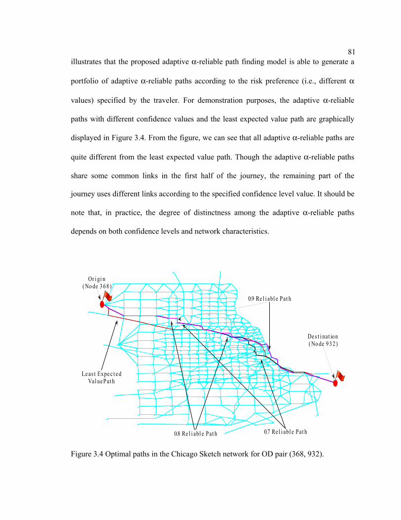
81illustrates that the proposed adaptive α-reliable path finding model is able to generate a

portfolio of adaptive α-reliable paths according to the risk preference (i.e., different α

values) specified by the traveler. For demonstration purposes, the adaptive α-reliable

paths with different confidence values and the least expected value path are graphically

displayed in Figure 3.4. From the figure, we can see that all adaptive α-reliable paths are

quite different from the least expected value path. Though the adaptive α-reliable paths

share some common links in the first half of the journey, the remaining part of the

journey uses different links according to the specified confidence level value. It should be

note that, in practice, the degree of distinctness among the adaptive α-reliable paths

depends on both confidence levels and network characteristics.

L e a s t E x p e c t e dV a l u e P a t h

O r i g i n ( N o d e 3 6 8 )

0.9 R e l i a b l e P a t h

D e s t i n a t io n ( N o d e 9 3 2 )

0.7 R e l i a b l e P a t h0.8 R e l i a b l e P a t h Figure 3.4 Optimal paths in the Chicago Sketch network for OD pair (368, 932).

82Table 3.4 Optimal solutions for the Chicago Sketch network of OD pair (368, 932)

Adaptive α-reliable path Least expected

value path α = 0.7 α = 0.8 α = 0.9

Node # Travel time (min) Node # Travel time

budget (min) Node # Travel time budget (min) Node # Travel time

budget (min) 368 112.87 368 120.67 368 123.47 368 134.31914 111.90 914 118.25 914 120.10 914 122.80389 108.65 389 114.80 389 116.55 389 119.20390 103.90 801 107.20 801 109.05 801 111.55388 91.80 802 101.20 802 103.10 802 105.50391 85.45 803 95.30 803 97.05 803 99.55392 80.85 807 90.50 807 92.30 807 94.90393 78.15 806 87.50 806 89.30 806 91.75394 74.95 710 84.60 710 86.30 710 88.90395 72.70 584 79.85 584 81.60 584 84.05396 69.30 588 75.25 588 77.00 588 79.45397 67.30 397 72.60 397 74.45 397 76.70604 66.20 398 70.50 398 72.10 398 74.60399 64.50 399 69.65 399 71.40 399 73.75537 60.50 537 65.55 537 67.25 537 69.45536 57.55 536 62.45 536 64.10 610 68.60438 55.65 438 60.20 438 61.60 615 65.65437 51.85 437 56.25 437 57.60 622 62.30436 49.05 556 52.90 556 54.25 555 59.20496 48.05 557 49.95 560 51.55 556 56.00495 45.65 559 47.25 561 49.05 560 53.40494 43.05 566 45.05 494 48.30 561 50.85493 41.10 500 43.45 563 46.10 494 50.05497 39.70 570 42.75 564 44.55 563 47.70498 39.05 572 40.10 565 43.00 564 46.20533 37.80 573 37.45 568 41.40 565 44.60532 36.55 528 35.10 574 39.30 568 42.90531 35.15 526 26.05 575 36.25 574 40.90529 33.98 527 20.45 581 33.55 575 37.70528 32.58 543 16.50 582 29.80 581 35.05526 23.98 903 15.55 541 26.80 582 31.25527 18.60 544 12.20 902 22.95 541 28.30543 14.93 515 11.65 542 20.70 902 24.40534 11.95 932 903 16.40 542 22.10515 10.45 544 13.00 903 17.65932 515 12.40 544 14.35

932 515 13.35 932

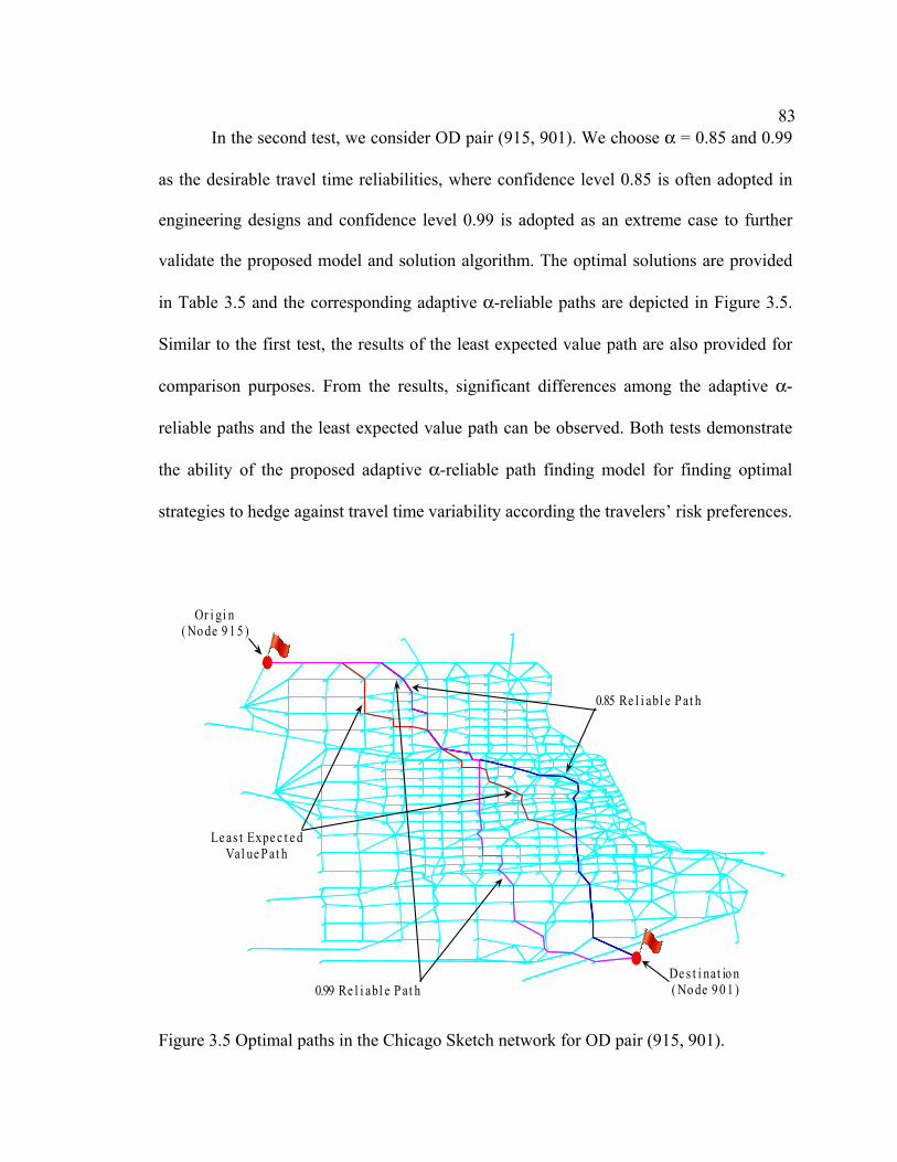
83In the second test, we consider OD pair (915, 901). We choose α = 0.85 and 0.99

as the desirable travel time reliabilities, where confidence level 0.85 is often adopted in

engineering designs and confidence level 0.99 is adopted as an extreme case to further

validate the proposed model and solution algorithm. The optimal solutions are provided

in Table 3.5 and the corresponding adaptive α-reliable paths are depicted in Figure 3.5.

Similar to the first test, the results of the least expected value path are also provided for

comparison purposes. From the results, significant differences among the adaptive α-

reliable paths and the least expected value path can be observed. Both tests demonstrate

the ability of the proposed adaptive α-reliable path finding model for finding optimal

strategies to hedge against travel time variability according the travelers’ risk preferences.

O r i g i n

( N o d e 9 1 5 )

D e s t i n a t io n ( N o d e 9 0 1 )

L e a s t E x p e c t e dV a l u e P a t h

0.85 R e l i a b l e P a t h

0.99 R e l i a b l e P a t h

Figure 3.5 Optimal paths in the Chicago Sketch network for OD pair (915, 901).

84Table 3.5 Optimal solutions for the Chicago Sketch network of OD pair (915, 901)

Adaptive α-reliable path Least expected value path α = 0.85 α = 0.99

Node # Travel time (min) Node # Travel time

budget (min) Node # Travel time budget (min)

915 135.03 915 146.03 915 153.58916 129.18 916 139.80 916 148.80917 123.38 917 133.80 917 141.85782 116.49 918 127.55 918 135.20787 110.94 783 120.80 783 128.85795 105.02 788 116.05 788 122.80799 100.28 790 113.35 790 120.85805 97.48 796 110.30 796 117.10804 94.61 800 107.50 800 115.25808 91.77 808 101.40 808 108.05584 85.50 584 94.70 584 101.30605 80.25 588 90.10 588 96.60607 77.75 397 87.65 397 93.55606 74.88 604 86.45 604 93.55403 73.68 399 84.75 606 90.60404 70.68 537 80.80 675 87.05405 69.76 536 77.65 677 84.35488 68.81 438 75.85 687 80.45487 66.40 437 72.00 689 77.90535 62.91 556 68.65 699 74.30486 62.65 557 65.65 701 71.95480 60.76 490 63.05 813 68.65479 59.59 631 61.85 472 66.55478 56.57 571 57.95 815 64.50477 54.27 637 55.70 821 61.45504 53.40 644 52.85 823 58.60505 50.17 646 49.75 828 55.85506 47.93 653 46.50 838 52.35507 44.35 655 43.05 454 50.75646 44.08 663 39.75 840 49.20653 41.15 665 36.40 847 44.55655 38.04 849 31.45 857 38.30663 35.10 859 25.30 885 31.15665 32.11 887 18.20 892 23.85849 27.54 893 11.80 897 19.35859 21.80 901 443 18.15887 15.33 898 13.65893 9.53 900 8.55901 901

85Conclusions

In this paper, an adaptive α-reliable path finding problem is introduced. It is to

adaptively determine a reliable path from a given origin to a given destination under an

uncertain environment, such that at each intermediate node (including the origin) the

desired reliability threshold α is satisfied and its corresponding travel time budget is

minimum. The adaptive α-reliable path finding problem has the ability to incorporate

both travelers' anticipation and real-time traffic information into the route choice decision

process. Thus, travelers' routing strategy can be dynamically adjusted and more accurate

estimation of their travel time budget can be acquired during the traveling period. It

allows more flexibility and better arrangement of their schedule and activities. The

problem is formulated as a chance constrained model, where the chance constraint

represents the travel time reliability requirement under a dynamic programming

framework. The properties of the proposed adaptive α-reliable path finding model are

explored in relation with the stochastic on-time arrival path finding model. Equivalency

of the two models is rigorously proved. By using the equivalence property, a discrete-

time solution algorithm is developed. The computational complexity of the proposed

algorithm is examined and its convergence properties are discussed. The proposed model

and solution algorithm are also demonstrated by numerical experiments using both a

small network and a large network.

In this study, the link travel time distributions are assumed to be independent. It

would be of interest to further study the situation with correlated link travel times.

Furthermore, the proposed path finding model may be adopted to describe the traveler's

86risk-averse route choice behavior. Therefore, it can be embedded as a subproblem in a

risk-based traffic equilibrium problem (e.g., Lo, Luo, and Siu, 2006; Shao et al., 2006).

That would be an interesting topic for further study.

References

Abdel-Aty, M., R. Kitamura, and P. Jovanis. 1995. Exploring route choice behavior using

geographical information system-based alternative routes and hypothetical travel time information input. Transportation Research Record 1493:74-80.

Bar-Gera, H. 2001. Website of transportation network test problems.

http://www.bgu.ac.il/~bargera/tntp. Bell, M. G. H., and Y. Iida. 1997. Transportation network analysis, John Wiley & Sons,

New York. 216 p. Bellman, E. 1958. On a routing problem. Quarterly of Applied Mathematics 16:87-90. Brownstone, D., A. Ghosh, T. F. Golob, C. Kazimi, and D. V. Amelsfort. 2003. Drivers’

willingness-to-pay to reduce travel time: Evidence from the San Diego I-15 congestion pricing project. Transportation Research Part A 37(4):373-387.

Cambridge Systematics, Inc., Texas Transportation Institute, University of Washington,

Dowling Associates. 2003. Providing a highway system with reliable travel times. NCHRP Report No. 20-58[3], Transportation Research Board, National Research Council, U.S.A.

Chen, A., and Z. Ji. 2005. Path finding under uncertainty. Journal of Advanced

Transportation 39(1):19-37. Dantzig, G. B. 1960. On the shortest route through a network. Management Science 6:

187-190. Dijkstra, E.W. 1959. A note on two problems in connection with graphs. Numerical

Mathematics 1:269-271. Fan, Y. Y., R. E. Kalaba, and J. E. Moore. 2005a. Shortest paths in stochastic networks

with correlated link costs. Computational Mathematics and Application 49:1549-1564.

87Fan, Y. Y., R. E. Kalaba, and J. E. Moore. 2005b. Arriving on time. Journal of

Optimization Theory and Application 127:497-513. FWHA. 2004. Traffic congestion and reliability trends and advanced strategies for

congestion mitigation. http://ops.fhwa.dot.gov/congestion_report_04 FHWA. 2006. Travel time reliability: Making it there on time, all the time. Report No.

70, Federal Highway Administration. Frank, H. 1969. Shortest paths in probabilistic graphs. Operations Research 17, pp.583-

599. Fu, L., and L. R. Rilett. 1998. Expected shortest paths in dynamic and stochastic traffic

networks. Transportation Research Part B 32:499-516. Hall, R. 1986. The fastest path through a network with random time-dependent travel

times. Transportation Science 20:182-188. Lam, T. 2000. The effect of variability of travel time on route and time-of-day choice.

Unpublished Ph.D. dissertation. University of California, Irvine. 174 p. Lo, H. K., X. W. Luo, and B. W. Y. Siu. 2006. Degradable transport network: Travel

time budget of travelers with heterogeneous risk aversion. Transportation Research B 40:792-806.

Loui, P. 1960. Optimal paths in graphs with stochastic or mulltidimensional weights.

Communications of ACM 26:670-676. Miller-Hooks, E., and H. Mahmassani. 2000. Least expected time paths in stochastic

time-varying transportation networks. Transportation Science 34:198-215. Mirchandani, P. B. 1976. Shortest distance and reliability of probabilistic networks.

Computers and Operations Research 3:347-355. Mirchadani, B. P., and H. Soroush. 1985. Optimal paths in probabilistic networks: A case

with temporary preference. Computers and Operations Research 12(4):365-383. Murthy, I., and S. Sarkar. 1996. A relaxation-based pruning technique for a class of

stochastic shortest path problems. Transportation Science 30(3):220-236. Nie, Y., and Y. Y. Fan. 2006. The arriving on time problem: A discrete algorithm that

ensures convergence. Transportation Research Record 1964: 193-200.

88Sen, S., R. Pillai, S. Joshi, and A. K. Rathi. 2001. A mean-variance model for route

guidance in advance traveler information systems. Transportation Science 35(1):37-49.

Shao, H., W. H. K. Lam, Q. Meng, and M. L. Tam. 2006. Demand-driven traffic

assignment problem based on travel time reliability. Transportation Research Record 1985: 220-230.

Sigal, C. E., A. A. B. Pritsker, and J. J. Solberg. 1980. The stochastic shortest route

problem. Operations Research 28:1122-1129. Sivakumar, R. A., and R. Batta. 1994. The variance-constrained shortest path problem.

Transportation Science 28:1122-1129. Small, K. A., R. Noland, X. Chu, and D. Lewis, 1999. Valuation of travel-time savings

and predictability in congested conditions for highway user-cost estimation. NCHRP Report No. 431, Transportation Research Board, National Research Council, U.S.A.

Waller, S. T., and A. K. Ziliaskopoulos. 2002. On the online shortest path problem with

limited arc cost dependencies. Networks 40:216-227. Yu, G. and J. Yang. 1998. On the robust shortest path problem. Computers and

Operations Research 25(6):457-268.

89CHAPTER 4

THE α-RELIABLE MEAN-EXCESS PATH FINDING MODEL IN

STOCHASTIC NETWORKS1

Abstract

In this paper, we propose an α-reliable mean-excess model for finding optimal

path in stochastic networks. This new model accounts for not only the reliability aspect

that the traveler wishes to arrive at his/her destination within the travel time budget, but

also the unreliability aspect of encountering worst travel times beyond the acceptable

travel time budget. The α-reliable mean-excess path finding model is consistent with the

commuters’ route choice behavior revealed in several recent empirical studies. That is,

commuters are not only interested in saving their travel time but also in reducing their

risk of being late. The proposed model is formulated as a stochastic mixed-integer

nonlinear programming problem. To solve this difficult problem, a double-relaxation

scheme is developed to find the α-reliable mean-excess paths. Illustrative examples and

numerical results are presented to demonstrate the proposed model and solution

procedure.

Introduction

Uncertainties are unavoidable in many decision-making problems. The path

finding problem is no exception. In a transportation network, travel times are highly

uncertain. The sources contributing to travel time variability could be exogenous and/or

1 Co-authored by Zhong Zhou and Anthony Chen

90endogenous (Cambridge Systematics et al., 2003). Exogenous sources refer to capacity

variations (e.g., traffic incidents, capacity degradations due to work zones and weather

conditions, traffic control device, etc.), which often lead to non-recurrent congestion

(Chen et al., 1999, 2002; Lo, Luo, and Siu, 2006; Al-Deek and Emam, 2006), while

endogenous sources refer to demand variations (e.g., travel demand fluctuations between

origin-destination pairs), which usually lead to recurrent congestion (Asakura and

Kashiwadani, 1991; Clark and Watling, 2005; Heydecker, Lam, and Zhang, 2007). The

resulting link/path travel time distributions often exhibit high asymmetry with long tails

when both recurrent and non-recurrent congestion occur simultaneously. Such travel time

variability introduces uncertainty for travelers such that they do not know exactly when

they will arrive at the destination. Thus, it is considered as a risk to a traveler making a

trip. Many stochastic path finding models in the literature hedge against travel time

variability by using the expected value model (e.g., Hall, 1986; Fu and Rilett, 1998;

Miller-Hooks and Mahmassani, 2000; Waller and Ziliaskopoulos, 2002; Fan, Kalaba, and

Moore, 2005a), which is unable to directly address the risk preferences of travelers

toward travel time variability on their route choice decisions. The path with the minimum

expected travel time may be risky for travelers who are more concerned about travel time

reliability when finding optimal paths in an uncertain environment.

Recently, various optimal path finding models have been developed to take travel

time variability into consideration. Sen et al. (2001) presented a mean-variance model to

seek a path with a minimal compromise value of the expected travel time and travel time

variance. Sivakumar and Batta (1994) also considered a similar routing strategy for

balancing the mean and variance of path travel times. However, the mean-variance model

91implies symmetrical or nearly symmetrical path travel time distribution, which is

generally not satisfied in practice. Recent empirical studies (Cambridge Systematics et

al., 2003; FHWA, 2006; van Lint, van Zuylen, and Tu, 2008) show that the link/path

travel time distributions could be highly skew. Using only the mean and variance of

travel time may not be sufficient to capture the characteristics of the path travel time

distribution accurately. Yu and Yang (1998) proposed a min-max model to identify a

robust path with the minimal possible longest path travel time. Similar approach under

the robust optimization framework was developed by Bertsimas and Sim (2003), where

the link travel time distributions are assumed to be symmetrical, bounded and

independent from each other. Both models recommend the optimal path to be the best

alternative in the worst situation. However, because of the probability of encountering the

longest travel time (worst situation) could be very low, the min-max model may provide

an overly conservative solution. On the other hand, Frank (1969) and Mirchandani (1976)

suggested the optimal path should be the path that maximizes the probability of realizing

a travel time less than a predefined travel time threshold. Sigal, Pritsker, and Solberg

(1980) considered optimality as the path that has the highest probability to be the shortest

one. Fan, Kalaba, and Moore (2005b) proposed the stochastic on-time arrival (SOTA)

problem under a dynamic programming framework to provide a portfolio of routing

strategies that maximize the probability of on-time arrival for a range of travel time

budgets. All these maximum probability models are equivalent to finding the most

reliable path that maximizes the travel time reliability (Bell and Iida, 1997). Chen and Ji

(2005) provided an alternative definition of optimality that allows the travelers to specify

a confidence level α for finding a reliable path with the minimum travel time budget such

92that the probability of the path travel time less than or equal to this budget is greater or

equal to α. Similar definition was proposed by Lu et al. (2006), where the travel time

budget is called the Time-at-Risk (TaR). The optimal path was determined by solving a

bi-objective mathematical program, which is to minimize a parameterized sum of the

expected path travel time and the path travel time budget defined by TaR. Zhou and Chen

(Chapter 3) proposed an adaptive α-reliable path finding problem that adaptively

determines a reliable path with the minimum travel time budget required to meet the user-

specified reliability threshold α. In fact, the concept of the travel time budget (or TaR)

adopted in the above models is analogous to the Value-at-Risk (VaR), which is defined as

a quantile of potential losses and by far the most widely applied risk measure in the

finance area (Szego, 2005). However, it has been determined that VaR is not even a

weakly coherent measure of risk (Artzner et al., 1999). Models using VaR are unable to

deal with the possibility that the losses associated with the worst scenarios are

excessively higher than the VaR and reduction of VaR may lead to stretch the tail

exceeding VaR (Yamai and Yoshiba, 2001). In the same spirit, travel time budget (or

TaR) may also be an inadequate risk measure, which is unable to evaluate the impacts of

the late trips. In other words, it does not assess the magnitude of the unacceptable travel

times exceeding the travel time budget; thus it may introduce an overwhelmingly high

trip times to travelers if it is adopted as a decision criterion for choosing an optimal path

under an uncertain environment.

From the travelers’ point of view, the α-reliable path finding model provides

travelers the answer to the question that concerns with the reliability aspect, such as “how

much time do I need to allow?” or “how reliable the trip is?” The report issued by FHWA

93(2006) documented that travelers, especially commuters, do add a 'buffer time' to their

expected travel time to ensure more frequent on-time arrivals when planning a trip.

However, considering only the reliability aspect may not be adequate to describe

travelers’ risk preferences under travel time variability. It does not address travelers’

concern about the unreliability aspect in their path selection decisions, such as “how bad

should I expect from the worse cases?”, where trip times longer than they expected would

be considered as “unreliable” or “unacceptable” (Cambridge Systematics et al., 2003).

Based on the recent empirical study on the Netherlands freeways (van Lint, van Zuylen,

and Tu, 2008), travel time distributions are not only very wide but also heavily skewed

with long tail. It has a significant impact on travelers facing unacceptable risk (i.e.,

unacceptable travel times). For example, it has been shown that about 5% of the “unlucky

drivers” incur almost five times as much delay as the 50% of the “fortunate drivers” on

densely used freeway corridors in the Netherlands. Therefore, it is highly desirable to

move forward by developing a new optimal path finding model that can better reflect the

travelers' risk preferences on both the reliability and unreliability aspects of travel time

variability (i.e., reducing the risk of encountering unacceptable travel times as well as

improving the likelihood of arriving on time). This motivates our present research.

In this paper, we present a new model called α-reliable mean-excess model, or

mean-excess model for short, for finding optimal path in stochastic networks. In contrast

to the α-reliable path finding model (Chen and Ji, 2005), which is to minimize the travel

time budget required to satisfy the user-specified confidence level α, the mean-excess

model attempts to minimize the path mean-excess travel time, which is the conditional

expectation of travel times beyond the travel time budget. Note that the mean-excess

94model also provides the endogenously determined travel time budget for a given

confidence level α specified by the traveler. This optimal path finding criterion can be

regarded as a combination of the buffer time measure that represents the reliability aspect

by determining the travel time budget required to ensure on-time arrival at least at a

confidence level α, and the tardy time measure that represents the unreliability aspect of

encountering worst travel times beyond the travel time budget (Cambridge Systematics et

al., 2003). It incorporates both the reliability and unreliability aspects of travel time

variability into the path finding decision criterion to simultaneously address both

questions: "how much time do I need to allow?" and "how bad should I expect from the

worse cases?" Furthermore, the definition of mean-excess travel time is consistent with

the conditional value-at-risk (CVaR) in the risk optimization literature (Rockafellar and

Uryasev, 2000). The CVaR is able to model flexible travel time distributions and has

been applied in various disciplines, such as portfolio optimization (Rockafellar and

Uryasev, 2000), facility location (Chen et al., 2006) and fleet allocation (Yin, 2007),

albeit not in the context of the stochastic path finding problem. Therefore, it is

meaningful to develop a path finding model that makes use of the CVaR measure to find

robust paths that explicitly consider the trade-off between the reliability and unreliability

aspects of travel time variability. Furthermore, compared to the α-reliable path finding

model of Chen and Ji (2005), the mean-excess model is computationally much easier to

solve, which makes it practical for applications such as route guidance systems based on

the Advanced Traveler Information Systems (ATIS), and also provides a meaningful

alternative to travelers who are concerned about both reliability and unreliability aspects

of travel time variability.

95The reminder of the paper is organized as follows. Section 2 presents the α-

reliable mean-excess path finding model and its mathematical formulation. An illustrative

example is used to demonstrate the differences of the proposed model with the expected

value model and the α-reliable (or travel time budget) model. In Section 3, a double-

relaxation scheme is developed for solving the proposed model. Numerical results are

presented in Section 4 to demonstrate the proposed model and solution procedure.

Finally, conclusions and further research directions are addressed in Section 5.

The α-reliable Mean-excess Path Finding Model

This section describes the α-reliable mean-excess model for finding optimal path

under travel time uncertainty. Notation is provided first for convenience, followed by the

definitions of mean-excess travel time, its mathematical programming formulation, and

illustrative examples to highlight the differences between the expected value model, the

α-reliable model, and the α-reliable mean-excess model.

Notation

),( AVG A stochastic network composed by nodes and links

V Set of nodes

A Set of links

r Origin (or source) node

s Destination (or terminal) node

)(nI Set of inbound links feeding into node n

)(nO Set of outbound links emanating from node n

96ijξ Random travel time on link (i , j)

ξ Vector of random link travel times ( ),, ijξξ =

ijx Decision variable, where ijx =1 means that link (i, j) is in

the path, and 0 otherwise

x Vector of decision variables, ( ), ,ijx x= , representing a

feasible path from origin r to destination s

( ),T x ξ Random travel time of path x (i.e., ( ),ij

ij ijx x

T x xξ ξ∈

= ∑ )

( ),xας ξ Travel time budget of path x with a predefined confidence

level α

( ),xαη ξ Mean-excess travel time of path x with a predefined

confidence level α

Definitions of mean-excess path and its mathematical formulation

To better reflect travelers’ risk preferences and allow a trade-off between the

reliable and unreliable aspects in path selection, we define the mean-excess path travel

time to be the optimal path finding criterion as follows.

Definition 1. (Mean-Excess Travel Time) The mean-excess travel time ( ),xαη ξ for a

path x with a predefined confidence level α is equal to the conditional expectation of the

travel times exceeding the corresponding path travel time budget ( ),xας ξ , i.e.,

( ) ( ) ( ) ( ), , | , ,x E T x T x xα αη ξ ξ ξ ς ξ= ≥⎡ ⎤⎣ ⎦ , (4.1)

97where ( ),T x ξ is the random travel time of path x from origin r to destination s, E[⋅] is

the expectation operator, and ( ),xας ξ is the minimum path travel time budget defined as

( ) ( )( ) , min | Pr ,x T T x Tας ξ ξ α= ≤ ≥ , (4.2)

where T is the path travel time threshold, α is a pre-determined confidence level

specified by the traveler, and ( )( )Pr ,T x ξ is the probability that the path travel time less

than the threshold is greater than or equal to α. A path that satisfies the above condition is

called the α-reliable path (Chen and Ji, 2005). The α-reliable path is meaningful for

travelers who are concerned with arriving at the destination within a certain level of

confidence while minimizing the travel time budget to satisfy the travel time reliability

constraint. This definition is also adopted in the models of Lo, Luo, and Siu (2006) and

Shao, Lam, and Tam (2006) to handle travel time variability in a network equilibrium

framework. Consequently, the mean-excess path as the optimal path can be defined as

follows.

Definition 2. (Mean-Excess Path) A path x is called the mean-excess path from origin r to

destination s if

( ) ( ) ( ) ( ) ( ) ( ) ( ) ( )

min , | , | , ,

min ', | ', | ', ',

x E T x T x x

x E T x T x x

α α

α α

η ξ ξ ξ ς ξ

η ξ ξ ξ ς ξ

≥⎡ ⎤⎣ ⎦

≤ ≥⎡ ⎤⎣ ⎦, (4.3)

for any path x' from origin r to destination s.

Based on Definition 1, by assuming the marginal cumulative distribution function

of path travel time on x is ( ),P x ξ , we have

( ) ( ) ( ) ( ), , | , ,x E T x T x xα αη ξ ξ ξ ς ξ= ≥⎡ ⎤⎣ ⎦

98

( )( ) ( )

( ), ,

1 , ,1 T x x

T x dP xαξ ς ξ

ξ ξα ≥

=− ∫ . (4.4)

Several possible travel time distributions, either exogenously or endogenously

defined in the transportation system, have been suggested in the literature to describe

travel time variability under an uncertain environment. One of the most popular and

straightforward assumptions is to assume the link travel time follows an independent or

multivariate normal distribution (e.g., Sen et al., 2001; Lo, Luo, and Siu, 2006, Shao,

Lam, and Tam, 2006). The advantage of the normal distribution assumption is obvious: it

enables the derivation of an analytical probability density function, which is also normal,

for each individual path. Thus, the correlation effects can be specified and the qualitative

analysis and computation can be easily performed.

However, the normal distribution assumption implies that link travel time is a

symmetrical distribution, which is generally not the case in practice. It is more reasonable

to adopt an asymmetrical distribution with some form of positive skewness to reflect the

actual travel time variability under recurrent and non-recurrent congestion (i.e., long tail

to the right). For example, Noland and Small (1995) adopted the exponential travel time

distribution for studying the morning commute problem. A family of distributions known

as the “Johnson curves”, including the lognormal distribution, was studied by Clark and

Watling (2005) to model the total network travel time under random demand, and by

Zhou and Chen (Chapter 6) for the comparative analysis of three network equilibrium

models under stochastic demand. Gamma type distributions were tested by Fan and Nie

(2006) for the stochastic optimal routing problem. A mixture of normal distribution was

suggested by Watling (2006) for modeling stochastic link/path travel times.

99Therefore, to illustrate the definitions of mean-excess travel time and its relation

to the travel time budget, a hypothetical distribution shown in Figure 4.1 is adopted. The

dash line represents the probability density function (PDF), while the solid line represents

the cumulative distribution function (CDF). Given a confidence level α, the travel time

budget is the minimum travel time threshold allowed by travelers such that the

corresponding CDF of actual travel time less than this threshold is at least α. The shaded

area (i.e., tail) represents all possible worse situations (late trips) that the actual travel

time is higher than the travel time budget, and the mean-excess travel time is the

conditional expectation of the late trips. Clearly, from the figure, we can see that the

travel time budget does not assess the magnitude of the possible travel time associated

with the worse situations and is unable to distinguish the situations where the actual

travel time is only a little bit higher than the travel time budget from those in which the

actual travel times are extremely higher. Therefore, the travel time budget only ensures

the reliability aspect of on-time arrival for a given confidence level α, while the mean-

excess travel time accounts for both the reliability aspect (i.e., travel time budget required

to ensure on-time arrival at a confidence level α) and the unreliability aspect of travel

time variability (i.e., encountering worse travel times beyond the travel time budget in the

tail).

Furthermore, note that Eq. (4.1) can be restated as:

( ) ( ) ( ) ( ) ( ) ( ), , , , | , ,x x E T x x T x xα α α αη ξ ς ξ ξ ς ξ ξ ς ξ= + − ≥⎡ ⎤⎣ ⎦ . (4.5)

Therefore, the mean-excess travel time can be decomposed into two individual

100

0 5 10 15 20 25 30

P r o

b a

b i

l i t

y D

e n

s i

t y

0 5 10 15 20 25 300

0.1

0.2

0.3

0.4

0.5

0.6

0.7

0.8

0.9

1

R o u t e T r a v e l T i m e

T r

a v

e l

T i

m e

R e

l i a

b i

l i t

y

C u m u l a t i v e P r o b a b i l i t y

P r o b a b i l i t y D e n s i t y

C o n f i d e n c e L e v e l

T r a v e l T i m e B u d g e t

M e a n E x c e s s T r a v e l T i m e

Figure 4.1 Illustration of the definitions of travel time budget and mean-excess travel

time. components. The first component is exactly the travel time budget of path x, which

reflects the reliability requirement (i.e., the confidence level α) of the travelers. The

second component is the expected value of the possible delays (or late trips) with

respectto the path travel time budget, which can be regarded as a kind of ‘expected delay’

for choosing the current path that reflects the unreliable impacts of travel time variability

induced by both recurrent and non-recurrent congestion. Clearly, the definition of mean-

excess travel time incorporates both the reliability and unreliability aspects in the path

selection process, while the existing path finding criteria only consider the reliability

aspect (e.g., α-reliable path, most reliable path) or consider neither aspect at all (e.g.,

mean path travel time). It enables the travelers to choose an optimal path such that the

corresponding travel time budget allows for on-time arrival with a predefined confidence

level and the possible risk of encountering worst travel times beyond the travel time

101budget is minimized.

According to definition 1 and definition 2, the mean-excess path finding model

can be formulated as a stochastic mixed-integer nonlinear programming (SMINLP)

problem as follows:

( ) ( )( ) ( )

( ), ,

1min , , ,1x

T x x

x T x dP xα

αξ ς ξ

η ξ ξ ξα ≥

=− ∫ (4.6)

( ) ( )

1. . 0 , ;

1ij ki

j O i k I i

i rs t x x i r i s

i s∈ ∈

∀ =⎧⎪− = ∀ ≠ ≠⎨⎪− ∀ =⎩

∑ ∑ , (4.7)

Ajixij ∈∀∈ ),(,1,0 , (4.8)

where

( ) ( )( ) , min | Pr ,x T T x Tας ξ ξ α= ≤ ≥ . (4.9)

From the above formulation, we can see that Eqs. (4.7) and (4.8) define the

feasibility of paths connecting from origin r to destination s. For any path x, the

corresponding travel time budget for a predefined confidence level α, which represents

the travelers’ concern about travel time reliability, is provided by Eq. (4.9). The objective

function given in Eq. (4.6) uses these paths that satisfy the travel time budget to further

examine the expected impacts of worst travel times in the tail (i.e., actual travel times

greater than the budget) in order to select an optimal path that considers both the

reliability aspect given by the travel time budget and the unreliability aspect of worst

travel times in the tails that are overwhelmingly higher than the allowable travel time

budget. Thus, the optimal mean-excess path is determined by minimizing the mean-

excess travel time of all feasible paths, i.e.

102 ( )

'arg min ',

x Xx xαη ξ

∈= . (4.10)

where X is the feasible path set defined by (4.7) - (4.8).

Illustrative example

The following illustrative example shows the differences among the expected

value, α-reliable, and mean-excess path finding models. A small hypothetical network

with three parallel paths connecting origin r and destination s is adopted in this

demonstration (see Figure 4.2). In this example, all travelers are assumed to have a

confidence level of α = 90%. In order to facilitate the presentation of the essential ideas,

the travel time distributions of the three paths are assumed to follow a log-normal

distribution ( ),Logn µ σ , whose PDF is shown as below:

( ) ( )2

2

ln1| , exp22

fξ µ

ξ µ σσξσ π

⎛ ⎞− −= ⎜ ⎟

⎜ ⎟⎝ ⎠

, 0ξ∀ > . (4.11)

The log-normal distribution is closely related to the normal distribution and has

been commonly adopted in practice to model a broad range of random processes. The

parameters µp and σp of the log-normal distribution for each path p (p = 1, 2, 3) are

shown in the Figure 4.2.

In this simple network where the path is equal to the link, the solution for the

expected value model can be derived analytically as follows.

( )2exp 2p p p pE Tπ µ σ⎡ ⎤= = +⎣ ⎦ , (4.12)

where pT represents the random travel time of path p (p = 1, 2, 3).

If the travelers adopt the α-reliable path finding model, the following

103

Figure 4.2 Hypothetical network used to illustrate the different path finding models. minimization problem should be considered (Chen and Ji, 2005):

min pς ( ). . Pr 90%p ps t T ς≤ ≥ . (4.13)

Under the assumption of the log-normal distributed path travel times, the travel

time budget each path can be analytically computed (Aitchison and Brown, 1957) as

follows:

( )( )1exp 2 2 1p p perfς σ α µ−= − + , (4.14)

where ( )1erf − ⋅ is the inverse of the Gauss error function defined as:

( ) ( )2

0

2 expx

erf x t dtπ

= −∫ . (4.15)

Now, suppose the travelers adopt the mean-excess path finding model. The

minimization problem given in Eqs. (4.6) - (4.9) can be rewritten as:

( )2

2

ln1 1min exp1 22p

p pp p

pp p

TT dT

Tς

µα σπ σ

∞⎛ ⎞− −⎜ ⎟⋅⎜ ⎟− ⋅⎝ ⎠

∫ ( ). . Pr 90%p ps t T ς≤ ≥ ,(4.16)

Under the assumption of the log-normal distributed path travel times and

104performing some calculus manipulations, the mean-excess travel time for each path can

be analytically presented as:

( )2

20

ln1 1 exp1 22

p pp p p p p

pp p

TT dT

T

µη ς ς

α σπ σ∞ +

⎛ ⎞− −⎜ ⎟⎡ ⎤= + − ⋅⎣ ⎦ ⎜ ⎟− ⋅⎝ ⎠

∫

( ) ( )( ) ( )2 1exp 2 2 2 1 1p p perfµ σ α σ α−= + ⋅Φ − ⋅ − + − , (4.17)

where ( )Φ ⋅ is the standard normal CDF, [ ]a a+ = if 0a > , and [ ] 0a + = otherwise.

The complete results derived analytically for all three path finding models are

provided in Table 4.1.

From Table 4.1, it is clear that different path finding models provide different

optimal paths, which reflect various risk preferences and considerations toward travel

time variability of the travelers. First, if the travelers are all risk-neutral, they only

consider the mean path travel time during their path selection process. Therefore, from

the expected value model column, they should choose path 3, which has the minimum

expected travel time of 7. However, path 3 is very risky, since it has the second highest

travel time budget and the highest mean-excess travel time. To ensure a 90% confidence

level of on-time arrival, travelers on path 3 have to allow a higher travel time budget than

those choosing path 2. Furthermore, even with the second highest travel time budget,

travelers on path 3 still have to experience the highest risk of facing a 10% probability

that the actual trip time will be longer than this travel time budget. Second, if the travelers

are risk-averse and concern more about the travel time reliability, they may choose a path

that gives them the minimum travel time budget. Under the α-reliable model column,

travelers will choose path 2. Therefore, travelers who plan to travel through path 2 may

105Table 4.1 Comparison of different path finding models

Path finding model

Expected value

model α-reliable model Mean-excess model

Decision criterion Mean travel time Travel time budget Mean-excess travel time Path 1 10 12.6389 13.9291 Path 2 8 12.1697 14.8037 Path 3 7 12.5119 17.0817 Optimal path Path 3 Path 2 Path 1

depart later than those who choose other paths and still ensure a 90% confidence level of

punctual arrival. However, comparing the expected value model column and the α-

reliable model column, it shows that the path with the least travel time budget may

introduce a higher mean-excess travel time. Therefore, for travelers who are concerned

with not only the travel time reliability, but also the unreliability of encountering worse

travel times, they may prefer to choose path 1. Though, by doing that, the corresponding

travel time budget is not the minimum, the expectation of the unacceptable travel times

greater than the allowable travel time budget is reduced by half compared to the α-

reliable model. In addition, they can still enjoy a 90% reliability of punctual arrival.

Solution Procedure

Solving stochastic mixed-integer nonlinear programming problems is generally

inefficient by using the general purpose integer programming software, especially when

the network size is large. Furthermore, even the joint link travel time distribution is

known with a PDF, an analytical expression of the path travel time distribution is usually

not available. Fortunately, as will be shown later, an analytical path travel time PDF is

106not necessary for solving the mean-excess path finding model described in the above

sections. It is sufficient to have a sampling technique, which generates random samples

according to the link travel time probability density function. Moreover, a double-

relaxation scheme is developed in this paper that uses the network structure to enhance

computational efficiency for practical implementation.

According to Rockafellar and Uryasev (2000), the minimization problem given in

Eqs. (4.6) - (4.9) is equivalent to minimizing the following program:

( ) ( ) ( )0,

1min , , ,1x

x T x dP xα

α α αςη ξ ς ξ ς ξ

α

+∞= + −⎡ ⎤⎣ ⎦− ∫ , (4.18)

where ας is a free decision variable, x X∈ , [ ]a a+ = if 0a > , and [ ] 0a + = otherwise.

It can be proved that the optimal value of the objective function ( ),xαη ξ is the

minimum mean-excess travel time, the corresponding optimal solution x gives the mean-

excess path, and the optimal value of the free decision variable ας is the travel time

budget of the mean-excess path. Moreover, the integral in Eq. (4.18) can be approximated

by sampling the random link travel times according to the specified PDFs. If the

sampling technique generates a collection of random link travel time vectors, 1, , Nξ ξ… ,

where ( ), ,k kijξ ξ= , for 1, ,k N= … , then Eq. (4.18) can be approximated as:

( ) ( ) ( )1

1min , ,1

Nk

x k

x T xNα α αη ξ ς ξ ς

α+

=

⎡ ⎤= + −⎣ ⎦− ∑ . (4.19)

To relax the nonnegative mapping ( ), kT x ξ ς+

⎡ ⎤−⎣ ⎦ , we introduce an auxiliary decision

variables kλ , for 1, ,k N= … . Then, Eq. (4.19) can be replaced by the following linear

program:

107

( ) ( ) 1

1min ,1

N

kx k

xNα αη ξ ς λ

α =

= +− ∑

subject to the following linear constraints:

ij

kk ij ij

x xx αλ ξ ς

∈

≥ −∑ and 0kλ ≥ , for 1, ,k N= … .

Note that, such relaxation is independent of the distribution assumption. It works

for both symmetrical and asymmetrical distributions (e.g., normal and non-normal).

However, solving large-scale mixed integer linear programs may still be time-

consuming using the general purpose mixed integer programming software. By utilizing

the network structure described by the flow conservation constraints given in Eq. (4.7),

we are able to perform another relaxation by replacing the 0-1 constraints in Eq. (4.8) by

0 1 ( , )ijx i j A≤ ≤ ∀ ∈ .

Therefore, by performing the sampling technique and the two relaxations, the mean-

excess path finding model can be finally reduced to a linear program as follows.

( ) ( ) 1

1min ,1

N

kx k

xNα αη ξ ς λ

α =

= +− ∑ (4.20)

. . ,ij

kk ij ij

x xs t x αλ ξ ς

∈

≥ −∑ for 1, ,k N= … , (4.21)

0kλ ≥ , for 1, ,k N= … , (4.22)

( ) ( )

10 , ;1

ij kij O i k I i

i rx x i r i s

i s∈ ∈

∀ =⎧⎪− = ∀ ≠ ≠⎨⎪− ∀ =⎩

∑ ∑ , (4.23)

0 1 ( , )ijx i j A≤ ≤ ∀ ∈ . (4.24)

As discussed above, our solution procedure includes two important relaxations.

108Therefore, we named it the double-relaxation method. In the following, we summarize

the main steps of the solution procedure:

Double-Relaxation Solution Procedure

Step 1. Solve the linear program (LP) in Eqs. (4.20) - (4.24) using any efficient LP

solvers (e.g., interior point algorithm).

Step 2. Identify a subset of paths with positive flows from the solution obtained in Step 1.

This is done by assigning link capacities corresponding to the solution, and

retrieving the flow-augmenting paths as a maximum-flow problem.

Step 3. Check the objective value of each path within the path set identified in Step 2.

Find the path with the minimum objective value as the optimal mean-excess path.

Remarks:

(1) As mentioned before, solving the mean-excess model (4.18) also provides the

corresponding travel time budget ας for the mean-excess path at the same time.

Therefore, the proposed solution procedure is able to acquire the optimal travel time

budget and the corresponding α-reliable path during the solution process. The only

additional operation required is to check the travel time budget of each path within

the path set, which can be performed in Step 3 along with the process of checking the

mean-excess travel time. This provides another way to solve the α-reliable path

finding problem that could be more efficient than the simulation-based genetic

algorithm (SGA) procedure suggested by Chen and Ji (2005).

(2) The proposed solution procedure is useful when the link travel time distributions are

already known. Furthermore, it can also directly deal with historical link travel time

data or stochastic travel time patterns described by a set of scenarios. In that case, the

109minimization program (4.19) can be replaced by

( ) ( ) ( )1

1min , ,1

Mk

kx k

x p T xα α αη ξ ς ζ ςα

+

=

⎡ ⎤= + ⋅ −⎣ ⎦− ∑ , (4.25)

where kp is the probability of occurrence for scenario kζ , 1, ,k M= … , and M is the

total number of scenarios. By relaxing the nonnegative mapping ( ), kT x ζ ς+

⎡ ⎤−⎣ ⎦ with

an auxiliary decision variable, kλ , Eq. (4.20) can be rewritten as

( ) ( ) 1

1min ,1

M

k kx k

x pα αη ξ ς λα =

= + ⋅− ∑ (4.26)

and the corresponding constraints (4.21) and (4.22) are also replaced by

,ij

kk ij ij

x xx αλ ξ ς

∈

≥ −∑ for 1, ,k M= …

0kλ ≥ , for 1, ,k M= … (4.27)

Therefore, by performing the proposed double-relaxation scheme, we can also obtain

the optimal mean-excess travel time as well as the optimal mean-excess path.

(3) The solution obtained in Step 1 may be all integers (0 or 1), or include some positive

fractions. In the former case (i.e. the solution is all integers), we already obtain the

optimal path from origin r to destination s with the minimum mean-excess travel

time. In the latter case, we need to identify a subset of paths that have positive flow

associated with the solution. The procedure in Step 2 has been adopted in Sen et al.

(2001) for determining optimal paths under the mean-variance model. It retrieves the

flow-augmenting paths in a maximum flow problem, where the link capacities

correspond to the solution of the relaxed LP problem. For more details of the

procedure, we refer to Murthy (1994).

110(4) To examine the computational complexity of the above solution procedure, we notice

that the linear program can be solved in polynomial time using the recently developed

interior point algorithms (Mehrotra, 1992). Furthermore, the solution procedure for

identifying the path set in Step 2 also runs in polynomial time (Sen et al., 2001;

Murthy, 1994). Therefore, the proposed double-relaxation solution procedure is

computationally efficient. It should be noted that the efficiency and accuracy of the

proposed solution algorithm will also be affected by different sampling techniques

and number of samples. In this study, a conventional Monte Carlo approach is

adopted for numerical experiments. However, other sampling techniques, such as

Quasi-Monte Carlo methods (e.g., Boyle, Broadie, and Glasserman, 1997; Kreinin et

al., 1998), could be incorporated to enhance the computational performance of the

proposed solution procedure.

Numerical Results

To demonstrate the proposed mean-excess model and solution procedure, two

networks are adopted in the numerical experiments. A small network is used first to

illustrate the mean-excess model and the correctness of the solution procedure. A

medium-sized network is then employed to demonstrate the applicability of the solution

procedure to larger networks. In our implementation, all codes are written in Matlab 7,

where a built-in interior point algorithm procedure is called for solving the relaxed linear

program. The numerical experiments are tested on a PC Workstation with 3.0 GHz CPU

and 2G memory.

111Small network

The first test network shown in Figure 4.3 is a 9-node grid network taken from

Chen and Ji (2005). In this network, there are four types of links and the travel times on

all four types of links are assumed to follow a normal distribution with similar means but

different variances (see Table 4.2). All possible paths from origin 1 to destination 9 are

also labeled and represented in the figure. The reason for choosing a normal distribution

in this numerical experiment is because it enables deriving analytical expressions of the

travel time distribution for each path. Therefore, we can solve the problem analytically

and use the results as a benchmark to compare the mean-excess model with the α-reliable

model and to validate the proposed double-relaxation solution procedure.

Based on the assumption of normally distributed link travel times, the path travel

time distributions are also normal. Therefore, the descriptive statistics of all the paths can

be analytically computed (Table 4.3).

According to the definitions of travel time budget and mean-excess travel time, it

is easy to derive the analytical form of path travel time budget and path mean-excess

travel time as below:

( )12 2 1p p erfς µ σ α−= + ⋅ − (4.28)

( )

( )( )21exp 2 12 1

pp p erf

ση µ α

π α−= + − −

− (4.29)

By assuming travelers' confidence level α increases from 0.5 to 0.9 with an

interval of 0.1, the corresponding path travel time budget and path mean-excess travel

time are listed in Table 4.4 and Table 4.5.

112

1 2 3

4 5 6

7 8 9

A A

A

A

Path 1(1-2-3-6-9)

Path 4(1-2-5-6-9)

Path 5(1-4-5-6-9)

Path 6(1-2-5-8-9)

Path 3(1-4-5-8-9)

B

B

B B

D

C

CD

Path 2(1-4-7-8-9)

Figure 4.3 Small network. Table 4.2 Link travel time distribution

Link Type Distribution (mean, variance) A Normal (200, 400) B Normal (207, 20) C Normal (202.5, 30) D Normal (198, 1500)

Table 4.3 Statistics of all paths

Path 1 (sec.)

Path 2 (sec.)

Path 3 (sec.)

Path 4 (sec.)

Path 5 (sec.)

Path 6 (sec.)

Mean 800 828 810 805 807.5 807.5 STD 28.28 28.77 28.46 28.37 28.42 28.42

The α-reliable paths and mean-excess paths for each confidence level are

provided in Table 4.4 and Table 4.5, where the corresponding optimal path travel time

113budget and optimal path mean-excess travel time are all marked in bold. From the two

tables above, the following observations can be drawn:

Different path finding criteria provide different optimal paths. It is easy to see that

path 1 would be the optimal path if the expected value model is adopted, which gives

the minimum mean travel time. However, path 1 may not be a reliable path under an

uncertain environment. For example, under a confidence level of 0.8, the optimal path

with the minimum travel time budget is path 4. Even the mean travel time of path 4 is

higher than that of path 1, travelers may still prefer path 4, which requires a lower

travel time budget in order to ensure a 80% reliability of on-time arrival. On the other

hand, to consider not only a 80% travel time reliability but also the unreliable aspect

(i.e., the impact of possible late arrivals with travel times higher than the travel time

budget) path 2 should be selected as the optimum since it has the minimal mean-

excess travel time.

The path travel time budget and path mean-excess travel time are non-decreasing

when the confidence level α increases. This observation is not surprising because, to

obtain a higher reliability, extra buffer times are needed.

Table 4.4 Analytical results of the α-reliable model for different confidence levels (α)

Confidence level (α)

Path 1 (sec.)

Path 2 (sec.)

Path 3 (sec.)

Path 4 (sec.)

Path 5 (sec.)

Path 6 (sec.)

α-reliable path

0.5 800.00 828.00 810.00 805.00 807.50 807.50 Path 1 0.6 810.13 830.27 823.97 812.43 818.69 818.69 Path 1 0.7 820.98 832.69 838.91 820.38 830.66 830.66 Path 4 0.8 833.66 835.53 856.40 829.68 844.67 844.67 Path 4 0.9 851.26 839.46 880.66 842.58 864.09 864.09 Path 2

114Table 4.5 Analytical results of the mean-excess model for different confidence levels (α)

Confidence level (α)

Path 1 (sec.)

Path 2 (sec.)

Path 3 (sec.)

Path 4 (sec.)

Path 5 (sec.)

Path 6 (sec.)

Mean-excess path

0.5 831.92 835.14 853.99 828.40 842.73 842.73 Path 4 0.6 838.63 836.64 863.25 833.32 850.15 850.15 Path 4 0.7 846.36 838.37 873.90 838.99 858.68 858.68 Path 2 0.8 855.99 840.52 887.18 846.05 869.31 869.31 Path 2 0.9 870.20 843.70 906.76 856.47 885.00 885.00 Path 2

Furthermore, we can observe that the path mean-excess travel time is always higher

than the corresponding path travel time budget. This observation is consistent with

Eq. (4.5), where an additional buffer time is added to the travel time budget to

account for the possibility of encountering worst travel times beyond the travel time

budget. In this way, the mean-excess model accounts for both reliability and

unreliability aspects rather than only the reliability aspect as in the α-reliable model

to minimize the expensive penalty of possible delays in the tail.

Now, using the analytical results as a benchmark, we can examine the validity of

the proposed double-relaxation solution procedure. Let's choose a sample size (N) of 300,

the generated augmented paths, travel time budgets and mean-excess travel times are

provided in Table 4.6. The α-reliable paths and mean-excess paths for each confidence

level are also listed in the table, where the corresponding optimal path travel time budget

and optimal path mean-excess travel times are marked in bold.

The results demonstrate the validity of the proposed solution procedure, which is

capable of finding the mean-excess paths with the optimal mean-excess travel time and

the α-reliable paths with the minimum travel time budget. Note that the proposed

solution procedure is applicable for the uncertain environment in practice, where the link

115Table 4.6 Numerical results of the 9-node network

Confidence level

Generated path

Travel time budget

α-reliable path

Mean-excess travel time

Mean-excess path

0.5 Path 1 798.39 832.46 Path 4 802.73 829.09 Path 6 806.41 842.24 Path 3 805.27

Path 1

849.94

Path 4

0.6 Path 1 809.94 839.57 Path 4 813.42 834.14 Path 5 812.47 848.71 Path 6 819.86 859.37 Path 2 830.54

Path 1

836.90

Path 4

0.7 Path 1 822.63 847.30 Path 4 822.09 839.37 Path 6 827.74 858.83 Path 3 836.96 869.22 Path 2 833.26

Path 4

838.56

Path 2

0.8 Path 1 831.67 857.56 Path 4 831.26 845.60 Path 5 841.55 869.99 Path 6 852.86 881.78 Path 2 836.16

Path 4

840.60

Path 2

0.9 Path 1 851.84 873.41 Path 4 840.76 855.04 Path 6 865.73 885.86 Path 3 876.67 900.35 Path 2 839.77

Path 2

843.18

Path 2

travel time distributions are generally asymmetric and have long tails (van Lint, van

Zuylen, and Tu, 2008). Under such cases, it may be quite difficult or even impossible to

derive the path travel time distributions and find the optimal path analytically.

In the following, we examine the computational performance of the proposed

double-relaxation solution procedure. First, we define the difference between the optimal

mean-excess travel time obtained from the proposed solution procedure ( optη ) and the

116one derived from the analytical method ( *

optη ) to be *opt op tη η− . Then, the CPU time

and the logarithm of the difference with respect to the sample size are plotted in Figure

4.4. Here, without loss of generality, we choose a confidence level of 80%.

From the figure, we can see that CPU time tends to increase when the sample size

increases. This is to be expected because more samples will introduce more constraints

during the relaxation process, thus increasing the size of the relaxed LP problem. On the

contrary, the difference *opt optη η− tends to decrease when the sample size increases.

0.0

0.5

1.0

1.5

2.0

2.5

3.0

50 100 150 200 250 300 350 400Sample Size

CPU

Tim

e (s

ec.)

-4.00

-3.60

-3.20

-2.80

-2.40

-2.00

Diff

eren

ce

CPU Time (sec.)Difference

Figure 4.4 CPU times and the common logarithm of the differences w.r.t. various sample size at α=80%.

117This is also anticipated, because more samples will enhance the representation of the

uncertain environment. Thus, it enables us to obtain a more accurate estimation of the

optimal solution.

Medium-sized network

In this section, the proposed model and solution procedure are demonstrated using

the Sioux Falls network (Leblanc, 1973), which is a medium-sized network with 76 links

and 24 nodes (see Figure 4.5). Without loss of generality, the link travel times are

assumed to follow a lognormal distribution with different means and variances. Links 6,

8, 10, 31, 12, 15, 16, and 19 (represented by the dotted lines) use the free-flow travel time

as the mean and 1/10 of the mean as the variance; links 13, 23, 25, 26, 28, 43, 46, and 47

(represented by the bold lines) use the free-flow travel time as the mean and 1/15 of the

mean as the variance; the remaining links use the free-flow travel time as the mean and

1/2 of the mean as the variance. Node 1 is selected as the origin and node 15 is chosen as

the destination. The reliability requirements (i.e., confidence level α) are tested from 0.5

to 0.9, and the sample size is set to be 400. The detailed solutions are provided in Table

4.7.

The results demonstrate that the proposed model and solution procedure do have

the capability of identifying the optimal path under asymmetric link travel time

distributions. Thus, it is able to take the travelers’ risk preferences into consideration

under more general situations than the traditional path finding models based on the

expected value model or the mean-variance model. By varying the reliability

requirements, the solution procedure can provide a portfolio of optimal paths that reflect

118

Figure 4.5 Sioux Falls network. the travelers’ various risk preferences. Furthermore, different path finding criteria may

provide different optimal paths. For example, under the same reliability requirement (e.g.,

80% confidence level), the mean-excess path could be different from the α-reliable path.

In each given confidence level, the optimal mean-excess travel time is always greater

than the optimal travel time budget due to the consideration of both reliability and

unreliability aspects. As a byproduct, the mean-excess model also obtains the travel time

budget of the α-reliable model in the proposed solution procedure with a few extra

119calculations (see Step 3 and remark 1 in the solution procedure section). Moreover, the

proposed solution procedure only explores part of the feasible path set. This implies that

the double-relaxation solution procedure has the potential to determine optimal paths in

real size networks efficiently, where the number of feasible paths may be numerous.

Conclusions

In this study, the α-reliable mean-excess path finding model is proposed to

consider both the travel time reliability requirement and the unreliability impact of

encountering worst travel times beyond the acceptable travel time budget. This optimal

Table 4.7 Computational results of Sioux Falls network

Confidence level

Generated paths in node sequence

Travel time budget (min.)

Mean-excess travel time (min.)

CPU time(second)

0.5 [1 3 4 11 10 15] 16.25 22.84 [1 3 4 11 14 15] 15.76 22.63

3.0823

0.6 [1 3 4 11 10 15] 17.71 24.33 [1 3 4 11 14 15] 17.02 24.19

[1 2 6 5 9 10 15] 22.04 30.48 [1 2 6 8 9 10 15] 21.23 31.70

3.5667

0.7 [1 3 4 11 10 15] 19.54 26.24 [1 3 4 11 14 15] 18.82 26.29 [1 2 6 5 9 10 15] 24.29 32.87 [1 2 6 8 9 10 15] 23.78 34.80

3.3443

0.8 [1 3 4 11 10 15] 21.87 29.02 [1 3 4 11 14 15] 21.54 29.26 [1 2 6 5 9 10 15] 26.86 36.61 [1 2 6 8 9 10 15] 27.47 39.53

4.2621

0.9 [1 3 4 11 10 15] 25.83 34.48 [1 3 4 11 14 15] 25.99 34.72 [1 2 6 5 9 10 15] 33.22 43.84

4.7293

120path finding criterion combines the buffer time measure, which represents the reliability

aspect by determining the travel time budget required to ensure on-time arrival with a

predefined confidence level α, and the tardy time measure, which represents the

unreliability aspect of encountering unacceptable delays. It addresses two concerns of the

travelers: “how much time do I need to allow?” and “how bad should I expect from the

worse cases?” Therefore, it is able to capture the travelers’ risk preferences more

completely and accurately, and better reflect the travelers’ decision process on path

selection. The model is useful for practical uncertain environments, where the travel time

distributions are generally nonnegative, asymmetric with long tails. A double-relaxation

solution procedure is also developed to solve the proposed model. Illustrative examples

and numerical experiments are conducted to demonstrate the features of the proposed

model and the validity and efficiency of the solution procedure. The flexibility of the

model and the efficiency of the solution procedure enable the determination of reliable

paths that can potentially be adopted in various real world applications, such as in-vehicle

route guidance system of ATIS.

In this study, the Monte Carlo simulation is adopted for solving the proposed

stochastic mixed-integer nonlinear program. It would be of interest to improve the

double-relaxation procedure by using more efficient simulation techniques. Furthermore,

the proposed mean-excess path finding model provides a pre-planned mean-excess path.

It would also be of interest to further extend the proposed model to enable travelers to

adaptively determine a α-reliable mean-excess path in a stochastic network, such as that

in Fan et al. (2005b) and Zhou and Chen (Chapter 3).

121References

Aitchison, J., and J. A. C. Brown. 1957. The lognormal distribution with special

reference to its uses in econometrics, Cambridge University Press, Cambridge, U.K. 194 p.

Al-Deek, H., and E. B. Emam. 2006. New methodology for estimating reliability in

transportation networks with degraded link capacities. Journal of Intelligent Transportation Systems 10(3): 117-129.

Artzner, P., F. Delbaen, J. M. Eber, and D. Heath. 1999. Coherent measures of risk.

Mathematical Finance 9:203-228. Asakura, Y., and M. Kashiwadani. 1991. Road network reliability caused by daily

fluctuation of traffic flow. European Transport, Highways & Planning, 19:73-84. Bell, M. G. H., and Y. Iida. 1997. Transportation network analysis, John Wiley & Sons,

New York. 216 p. Bertsimas, D., and M. Sim. 2003. Robust discrete optimization and network flows.

Mathematical Programming Ser. B 98:49-71. Boyle, P. P., M. Broadie, and P. Glasserman. 1997. Monte Carlo methods for security

pricing. Journal of Economic Dynamics and Control 21: 1267-1321. Cambridge Systematics, Inc., Texas Transportation Institute, University of Washington,

Dowling Associates. 2003. Providing a highway system with reliable travel times. NCHRP Report No. 20-58[3], Transportation Research Board, National Research Council, U.S.A.

Chen, A., and Z. Ji. 2005. Path finding under uncertainty. Journal of Advanced

Transportation 39(1):19-37. Chen, A., H. Yang, H. K. Lo, and W. Tang. 1999. A capacity related reliability for

transportation networks. Journal of Advanced Transportation 33(2):183-200. Chen, A., H. Yang, H. K. Lo, and W. H. Tang. 2002. Capacity reliability of a road

network: An assessment methodology and numerical results. Transportation Research Part B 36:225-252.

Chen, G., M. S. Daskin, Z. J. M. Shen, and S. Uryasev, 2006. The α-reliable Mean-

Excess Regret Model for Stochastic Facility Location Modeling, Naval Research Logistics 53:617-626.

122Clark, S. D., and D. Watling. 2005. Modeling network travel time reliability under

stochastic demand. Transportation Research Part B 29(2):119-140. Fan, Y. Y., R. E. Kalaba, and J. E. Moore. 2005a. Shortest paths in stochastic networks

with correlated link costs. Computational Mathematics and Application 49:1549-1564.

Fan, Y. Y., R. E. Kalaba, and J. E. Moore. 2005b. Arriving on time. Journal of

Optimization Theory and Application 127:497-513. Fan, Y. Y., and Y. Nie. 2006. Optimal routing for maximizing the travel time reliability.

Networks and Spatial Economics 6 (3):333-344. FHWA. 2006. Travel time reliability: Making it there on time, all the time. Report No.

70, Federal Highway Administration. Frank, H. 1969. Shortest paths in probabilistic graphs. Operations Research 17:583-599. Fu, L., and L. R. Rilett. 1998. Expected shortest paths in dynamic and stochastic traffic

networks. Transportation Research Part B 32:499-516. Hall, R. 1986. The fastest path through a network with random time-dependent travel

times. Transportation Science 20:182-188. Heydecker, B. G., W. H. K. Lam, and N. Zhang. 2007. Use of travel demand satisfaction

to assess road network reliability. Transportmetrica 3(2): 139-171. Kreinin, A., L. Merkoulovitch, D. Rosen, and Z. Michael. 1998. Measuring portfolio risk

using quasi Monte Carlo Methods. ALGO Research Quarterly 1(1): 17-25. LeBlanc, L. J. 1973. Mathematical programming algorithms for large-scale network

equilibrium and network design problems. Unpublished PhD thesis, Northwestern University, Evanston IL.

Lo, H.K., X. W. Luo, and B. W. Y. Siu. 2006. Degradable transport network: Travel time

budget of travelers with heterogeneous risk aversion. Transportation Research B 40: 792-806.

Lu, J., F. Yang, X. Ban, and B. Ran. 2006. Moments analysis for improving decision

reliability based on travel time. Journal of the Transportation Research Board 1968:109-116.

Mehrotra, S. 1992. On the implementation of a primal-dual interior point method. SIAM

Journal on Optimization 2:575-601.

123Miller-Hooks, E., and H. Mahmassani. 2000. Least expected time paths in stochastic

time-varying transportation networks. Transportation Science 34:198-215. Mirchandani, P. B. 1976. Shortest distance and reliability of probabilistic networks.

Computers and Operations Research 3:347-355. Murthy, K. G. 1994. Network Flow Programming. John Wiley&Sons, New York. 632 p Noland, R., and K. A. Small. 1995. Travel time uncertainty, departure time choice, and

the cost of morning commutes. Transportation Research Record 1493:150-158. Rockafellar, R. T., and S. Uryasev. 2000. Optimization of conditional value-at-risk.

Journal of Risk 2(3):21-41. Sen, S., R. Pillai, S. Joshi, and A. K. Rathi. 2001. A mean-variance model for route

guidance in advance traveler information systems. Transportation Science 35 (1):37-49.

Shao, H., W. H. K. Lam, and M. L. Tam. 2006. A reliability-based stochastic traffic

assignment model for network with multiple user classes under uncertainty in demand. Network and Spatial Economics 6: 173-204.

Sigal, C. E., A. A. B. Pritsker, and J. J. Solberg. 1980. The stochastic shortest route

problem. Operations Research 28:1122-1129. Sivakumar, R. A., and R. Batta. 1994. The variance-constrained shortest path problem.

Transportation Science 28:1122-1129. Szego, G. 2005. Measures of risk. European Journal of Operational Research, 163:5-19. van Lint, J. W. C., H. J. van Zuylen, and H. Tu. 2008. Travel time unreliability on

freeways: Why measures based on variance tell only half the story. Transportation Research Part A 42(1): 258-277.

Waller, S.T., and A. K. Ziliaskopoulos. 2002. On the online shortest path problem with

limited arc cost dependencies. Networks 40:216-227. Watling, D. 2006. User equilibrium traffic network assignment with stochastic travel

times and late arrival penalty. European Journal of Operational Research 175:1539-1556.

Yamai, Y., and Y. Yoshiba. 2001. On the validity of value-at-risk: Comparative analysis

with expected shortfall. Bank of Japan. IMES Discussion Paper 2001-E-4.

124Yin, Y. 2007. A Scenario-based Model for Fleet Allocation of Freeway Service Patrols,

Network and Spatial Economics. Published online first http://www.springerlink.com/content/a82374380x714302/

Yu, G., and J. Yang. 1998. On the robust shortest path problem. Computers and

Operations Research 25(6):457-268.

125CHAPTER 5

THE α-RELIABLE MEAN-EXCESS TRAFFIC EQUILIBRIUM MODEL

WITH STOCHASTIC TRAVEL TIMES1

Abstract

In this paper, we propose a new model called the α-reliable mean-excess traffic

equilibrium model or the mean-excess traffic equilibrium (METE) model for short that

explicitly considers both reliability and unreliability aspects of travel time variability in

the route choice decision process. In contrast to the travel time budget (TTB) models that

consider only the reliability aspect defined by TTB, this new model hypothesizes that

travelers are willing to minimize their mean-excess travel times (METT) defined as the

conditional expectation of travel times beyond the TTB. As a route choice criterion,

METT can be regarded as a combination of the buffer time measure that ensures the

reliability aspect of on-time arrival at a confidence level α , and the tardy time measure

that represents the unreliability aspect of encountering worst travel times beyond the

acceptable travel time allowed by TTB. It addresses both questions of “how much time

do I need to allow?” and “how bad should I expect from the worse cases?” Therefore,

travelers' route choice behavior can be considered in a more accurate and complete

manner in a network equilibrium framework to reflect their risk preferences under an

uncertain environment. The METE model is formulated as a variational inequality

problem and solved by a route-based traffic assignment algorithm via the self-adaptive

alternating direction method. Some qualitative properties of the model are rigorously

1 Co-authored by Zhong Zhou and Anthony Chen

126proved. Illustrative examples are also presented to demonstrate the characteristics of the

model as well as its differences compared to the recently proposed travel time budget

models.

Introduction

Uncertainty is unavoidable in real life. It surrounds all aspects of decision-making

and affects our daily life as well as the society. In transportation, uncertainty is a critical

and inseparable part of many problems. For example, the road network is one of the

systems that serves the travel demands in order to connect people engaged in various

activities (e.g., work, traveling, shopping, etc.) at different locations. The uncertainty of

network travel times exists in both supply side (roadway capacity variation) and demand

side (travel demand fluctuation). Figure 5.1 provides an illustration of various sources of

uncertainty that contribute to travel time variability. From the figure, we can observe that

several exogenous sources of uncertainty exist in the supply side. Weather conditions

refer to environmental conditions that can lead to changes in traveler behavior. For

example, travelers may lower their speeds or increase their headways (spacing between

vehicles) due to reduced visibility when fog, rain or snow is present. Traffic incidents,

such as car crashes, breakdowns or debris in lanes, often disrupt the normal flow of

traffic. Work zones are construction activities on the roadways that usually introduce

physical changes to the highway environment. The number or width of lanes may be

changed, shoulders may be eliminated, or roadways may be temporarily closed. Delays

caused by work zones have been regarded as one of the most frustrating conditions that

travelers encounter on their trips. Traffic control devices, such as signal timing and ramp

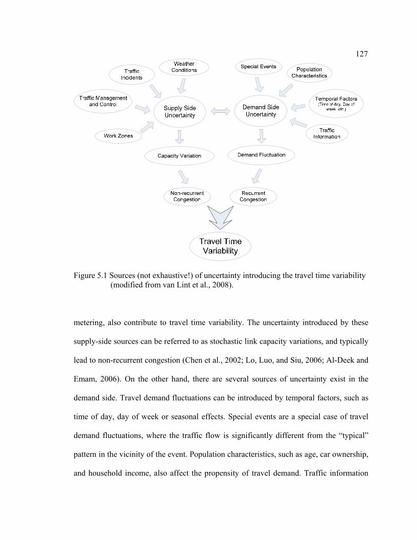
127

Figure 5.1 Sources (not exhaustive!) of uncertainty introducing the travel time variability (modified from van Lint et al., 2008).

metering, also contribute to travel time variability. The uncertainty introduced by these

supply-side sources can be referred to as stochastic link capacity variations, and typically

lead to non-recurrent congestion (Chen et al., 2002; Lo, Luo, and Siu, 2006; Al-Deek and

Emam, 2006). On the other hand, there are several sources of uncertainty exist in the

demand side. Travel demand fluctuations can be introduced by temporal factors, such as

time of day, day of week or seasonal effects. Special events are a special case of travel

demand fluctuations, where the traffic flow is significantly different from the “typical”

pattern in the vicinity of the event. Population characteristics, such as age, car ownership,

and household income, also affect the propensity of travel demand. Traffic information

128provided by Advanced Traveler Information Systems (ATIS) can also influence the

travelers’ trip decision, including their departure time, destination, mode, and route

choice, which consequently affect the traffic flow pattern. These demand variations

usually lead to recurrent congestion (Asakura and Kashiwadani, 1991; Clark and Watling,

2005). There are also complex interactions between the supply-side and demand-side

sources of uncertainty. For example, bad weather may reduce roadway capacity in the

network, and may at the same time change the spatial and temporal pattern of travel

demand, because travelers may decide to change their departure time, choose a different

route, or even cancel the trip. In short, these uncertain events result in the variation of

traffic flow, which directly contributes to the spatial and temporal variability of network

travel times. Such travel time variability introduces uncertainty for travelers such that

they do not know exactly when they will arrive at the destination. Thus, it is considered

as a risk to a traveler making a trip.

The effects of the travel time variability on travelers’ route choice behaviors have

been studied by several empirical surveys (Abdel-Aty, Kitamura, and Jovanis, 1995;

Small et al., 1999; Lam, 2000; Brownstone et al., 2003; Cambridge Systematics, et al.,

2003; Recker et al., 2005). Abdel-Aty, Kitamura, and Jovanis (1995) found that travel

time reliability was either the most or second most important factor for most commuters.

In the study by Small et al. (1999), they found that both individual travelers and freight

carriers were strongly averse to scheduling mismatches. For this reason, they were

willing to pay a premium to avoid congestion and to achieve greater reliability in travel

times. From the two value-pricing projects in Southern California, Lam (2000) and

Brownstone et al. (2003) also consistently found that travelers were willing to pay a

129substantial amount to reduce variability in travel time. Another study conducted by

Recker et al (2005) on the freeway system in Orange County, California observed that: (i)

both travel time and travel time variability were higher in peak hours than non-peak hours;

(ii) both travel time and travel time variability were much higher in winter months than in

other seasons; and (iii) travel time and travel time variability were highly correlated.

According to these observations, they suggested that commuters preferred departing

earlier to avoid the possible delays caused by travel time variability. These empirical

studies revealed that travelers considered travel time variability as a risk in their route

choice decisions. They are interested in not only travel time saving but also the travel

time variability reduction to minimize risk. Thus, it is suffice to say travel time variability

is a significant factor for travelers when making their route choice decisions under risk or

circumstances where they do not know with certainty about the outcome of their

decisions. Furthermore, a recent empirical study conducted by van Lint et al. (2008)

reveals that the travel time distribution is not only very wide but also heavily skewed

with a long fat tail. For example, it has been shown that about 5% of the “unlucky

drivers” incur almost five times as much delay as the 50% of the “fortunate drivers” on

the densely used freeway corridors in the Netherlands. The consequence of these heavily

skewed travel times on the right tail (i.e., the late trips with unacceptable travel times)

may be much more serious than those of modest delays, and it has a significant impact on

travelers’ route choice behavior.

However, travel time variability is not considered in the traditional user

equilibrium (UE) model, where travelers are all assumed to be risk-neutral and the route

choice decisions are based solely on the expected travel time. To model the route choice

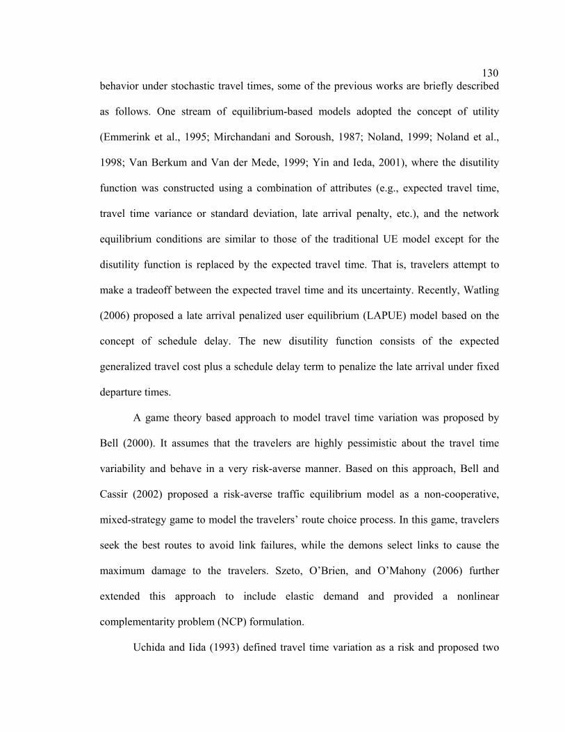
130behavior under stochastic travel times, some of the previous works are briefly described

as follows. One stream of equilibrium-based models adopted the concept of utility

(Emmerink et al., 1995; Mirchandani and Soroush, 1987; Noland, 1999; Noland et al.,

1998; Van Berkum and Van der Mede, 1999; Yin and Ieda, 2001), where the disutility

function was constructed using a combination of attributes (e.g., expected travel time,

travel time variance or standard deviation, late arrival penalty, etc.), and the network

equilibrium conditions are similar to those of the traditional UE model except for the

disutility function is replaced by the expected travel time. That is, travelers attempt to

make a tradeoff between the expected travel time and its uncertainty. Recently, Watling

(2006) proposed a late arrival penalized user equilibrium (LAPUE) model based on the

concept of schedule delay. The new disutility function consists of the expected

generalized travel cost plus a schedule delay term to penalize the late arrival under fixed

departure times.

A game theory based approach to model travel time variation was proposed by

Bell (2000). It assumes that the travelers are highly pessimistic about the travel time

variability and behave in a very risk-averse manner. Based on this approach, Bell and

Cassir (2002) proposed a risk-averse traffic equilibrium model as a non-cooperative,

mixed-strategy game to model the travelers’ route choice process. In this game, travelers

seek the best routes to avoid link failures, while the demons select links to cause the

maximum damage to the travelers. Szeto, O’Brien, and O’Mahony (2006) further

extended this approach to include elastic demand and provided a nonlinear

complementarity problem (NCP) formulation.

Uchida and Iida (1993) defined travel time variation as a risk and proposed two

131risk assignment models. Both models are established using the concept of effective travel

time, which is defined as the mean travel time plus a safety margin. Lam and Chan (2005)

argued that travelers should consider both travel time and travel time reliability for their

route choices. Thus, a path preference index (PI) that combines the path travel time index

(TI) and the path travel time reliability index (RI) is proposed to be the criterion of route

choices. Lo and Tung (2003) proposed a probabilistic user equilibrium (PUE) model,

where travel time variability is introduced by day-to-day stochastic link degradation with

predefined link capacity distributions. Lo, Luo, and Siu (2006) extended this approach by

incorporating the concept of travel time budget (TTB) to develop the within budget time

reliability (WBTR) model. Different from Uchida and Iida’s (1993) definition, TTB is

defined by a travel time reliability chance constraint, such that the probability that travel

time exceeds the budget is less than a predefined confidence level α specified by the

traveler to represent his/her risk preference. This definition is similar to that defined by

Chen and Ji (2005), where the route with the minimum TTB is termed “α-reliable route”.

Therefore, each commuter learns the travel time variations through his/her daily

commutes and chooses a route that minimizes his/her TTB. Later, Siu and Lo (2006)

extended the WBTR model to take traveler’s perception variation into consideration. By

assuming travel time variation is induced by daily travel demand variation instead of

capacity degradation, Shao et al. (2006) extended the PUE model and proposed a demand

driven travel time reliability-based user equilibrium (DRUE) model. The DRUE model

was further extended to a reliability-based stochastic user equilibrium (RSUE) model to

account for both perception error and multiple user classes (Shao, Lam, and Tam, 2006).

The core idea behind the travelers’ route choice behavior of the above models (Lo, Luo,

132and Siu, 2006; Shao, Lam, and Tam, 2006; Siu and Lo, 2006) is based on the concept of

TTB, which is defined as the average travel time plus an extra buffer time as an

acceptable travel time, such that the probability of completing the trip within the TTB is

no less than a predefined reliability threshold (or a confidence level α). In fact, the

concept of TTB is analogous to the Value-at-Risk (VaR), which is by far the most widely

applied risk measure in the finance area (Szego, 2005). However, it has been determined

that VaR is not even a weakly coherent measure of risk (Artzner et al., 1997, 1999).

Models using VaR is unable to deal with the possibility that the losses associated with the

worst scenarios are excessively higher than the VaR, and reduction of VaR may lead to

stretch of tail exceeding VaR (Larsen, Mausser, and Uryasev, 2002; Yamai and Yoshiba,

2001). In the same spirit, TTB may also be an inadequate risk measure, which could

introduce overwhelmingly high trip times (i.e., unreliability aspect of travel time

variability) to travelers if it is used solely as a route choice criterion in the network

equilibrium based approach.

Furthermore, to describe travelers' route choice decision process under travel time

variability, considering only the reliability aspect (i.e., buffer time or acceptable travel

time defined by TTB) may not be adequate to describe travelers’ risk preferences. On the

one hand, the reports issued by the Federal Highway Administration (FHWA, 2004, 2006)

documented that travelers, especially commuters, do add a 'buffer time' (or safety margin)

to their expected travel time to ensure more frequent on-time arrivals when planning a

trip. It represents the reliability aspect in the travelers' route choice decision process. On

the other hand, the impacts of late arrival and its explicit link to the travelers' preferred

arrival time were also examined in the literature (e.g., Noland et al., 1998; Noland, 1999;

133Hall, 1993; Porter, Wright and Dale, 1996) and appreciated as the ‘value’ of unreliability

(Watling, 2006). It represents travelers' concern of the unreliability aspect of travel time

variability in their route choice decision process, where trip times longer than they

expected would be considered as ‘unreliable’ or ‘unacceptable’ (Cambridge Systematics

et al., 2003). Therefore, it is reasonable to incorporate both reliability and unreliability

aspects of travel time variability into the network equilibrium model to describe travelers’

route choice behavior under stochastic travel times.

In this paper, we present a new α-reliable mean-excess traffic equilibrium model

or mean-excess traffic equilibrium (METE) model for short that explicitly considers both

reliability and unreliability aspects of travel time variability in the route choice decision

process. In contrast to the TTB models (Lo, Luo, and Siu, 2006; Shao et al., 2006; Shao,

Lam, and Tam, 2006; Siu and Lo, 2006) that consider only the reliability aspect defined

by TTB, this new model hypothesizes that travelers are willing to minimize their mean-

excess travel time (METT) defined as the conditional expectation of travel times beyond

the TTB. As a route choice criterion, METT can be regarded as a combination of the

buffer time measure that ensures the reliability of on-time arrival, and the tardy time

measure that represents the unreliability impacts of excessively late trips (Cambridge

Systematics et al., 2003). It incorporates both reliability and unreliability aspects of travel

time variability to simultaneously address both questions of "how much time do I need to

allow?" and "how bad should I expect from the worse cases?" Therefore, travelers' route

choice behavior can be considered in a more accurate and complete manner in a network

equilibrium framework to reflect their risk preferences under an uncertain environment.

Furthermore, the definition of METT is consistent with the conditional value-at-risk

134(CVaR) measure in the literature (Rockafellar and Uryasev, 2000, 2002) for risk

optimization. It has been recognized as a good alternative measure of risk due to its

coherent mathematical characteristics, and it is suitable for modeling flexible travel time

distributions, including non-symmetric and heavy tailed distributions. In addition, CVaR

has been applied in various fields, such as portfolio optimization (Rockafellar and

Uryasev, 2002), facility location (Chen et al., 2006) and fleet allocation (Yin, 2007),

albeit not in the context of traffic equilibrium problem under uncertainty.

The remainder of the paper is organized as follows. In Section 2, the concept of

mean-excess travel time in a stochastic network is introduced and the mean-excess traffic

equilibrium model is proposed, where the model is formulated as a variational inequality

(VI) problem. Some properties and analytical results of the model and formulation are

also presented. In Section 3, a route-based traffic assignment algorithm based on the self-

adaptive alternating direction method is developed to determine the equilibrium flow

pattern. In Section 4, numerical examples are presented to illustrate the features of the

proposed model, to compare with other related user equilibrium models, and to

demonstrate the applicability of the solution procedure. Finally, conclusions and

recommendations for future research are given in Section 5.

The Mean-Excess Traffic Equilibrium Model

This section describes the METE model for determining the equilibrium flow

pattern under stochastic travel times. Notation is provided first for convenience, followed

by the definition of mean-excess travel time, an illustrative example to highlight the

differences of using the expected travel time, the TTB, and the METT as a route choice

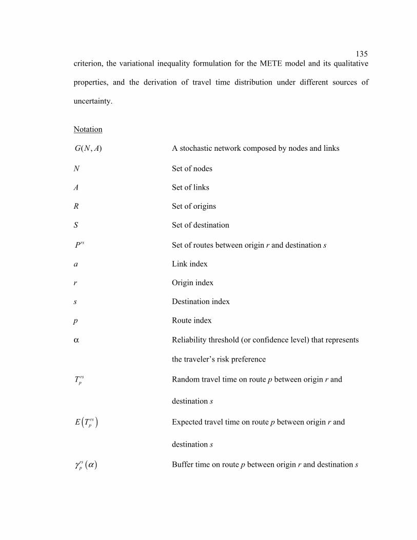
135criterion, the variational inequality formulation for the METE model and its qualitative

properties, and the derivation of travel time distribution under different sources of

uncertainty.

Notation

),( ANG A stochastic network composed by nodes and links

N Set of nodes

A Set of links

R Set of origins

S Set of destination

rsP Set of routes between origin r and destination s

a Link index

r Origin index

s Destination index

p Route index

α Reliability threshold (or confidence level) that represents

the traveler’s risk preference

rspT Random travel time on route p between origin r and

destination s

( )rspE T Expected travel time on route p between origin r and

destination s

( )rspγ α Buffer time on route p between origin r and destination s

136required to ensure on-time arrival at a confidence level α

rspξ Travel time budget (i.e., expected travel time + buffer time)

on route p between origin r and destination s required to

ensure on-time arrival at a confidence level α

rspη Mean-excess travel time on route p between origin r and

destination s

η Vector of mean-excess route travel times ( ), ,Trs

pη… …

rsπ Minimal mean-excess travel time between origin r and

destination s

at Mean travel time on link a

2aσ Variance of travel time on link a

rsq O-D demand between origin r and destination s

q Vector of O-D demands ( ), ,Trsq… …

rspf Flow on route p between origin r and destination s

f Vector of route flows ( ), ,Trs

pf… …

Λ OD-Route incidence matrix

av Flow on link a

rspaδ⎡ ⎤∆ = ⎣ ⎦ Route-link incidence matrix, where 1rs

paδ = if route p from

origin r to destination s uses link a, and 0 otherwise

137Definition of mean-excess travel time

In this study, travelers are assumed to have knowledge of the distribution of the

travel time variability. In practice, this kind of knowledge can be acquired from various

sources, such as their past commuting experiences or advanced traveler information

systems (ATIS). Travelers then incorporate this information into their route choice

decisions along with their own risk-preferences to reach a long-term habitual equilibrium

flow pattern. Therefore, to study the user equilibrium problem, the key factor here is to

understand the travelers’ route choice behavior under travel time variability. In this

section, we will illustrate the concept of METT (i.e., analogous to the Conditional Value-

at-Risk (CVaR) measure used in financial engineering) adopted as a route choice

criterion in a traffic equilibrium framework and demonstrate its differences with the

travel time budget (TTB) criterion adopted in many recent developed traffic equilibrium

models to consider the reliability aspect of travel time variability in the route choice

decision process.

As mentioned above, travelers are unable to accurately estimate the travel time

from their origin to destination due to travel time variability. This is considered as a risk

associated with their route choice decisions. According to Mirchandani and Soroush

(1987), travelers making route choice decisions under an uncertain environment can be

categorized into three groups according to their attitudes toward risk (e.g., risk-prone,

risk-neutral and risk-averse). In the traditional UE model, travelers are assumed to be

risk-neutral since they make their route choice decisions solely based on the expected

travel time ( )rspE T , where rs

pT is the random travel time on route p between origin r and

destination. However, recent empirical studies (Small et al., 1999; Lam, 2000;

138Brownstone et al., 2003; Liu, Recker, and Chen, 2004; de Palma and Picard, 2005;

Cambridge Systematics et al., 2003; FHWA, 2004, 2006) revealed that most travelers are

actually risk-averse. They are willing to pay a premium to avoid congestion and minimize

the associated risk.

By considering the travel time reliability requirement, travelers are searching for a

route such that the corresponding TTB allows for on-time arrival with a predefined

confidence level α (Lo, Luo, and Siu, 2006; Siu and Lo, 2006; Shao et al., 2006).

Meanwhile, they are also considering the impacts of excessively late arrival (i.e., the

unreliable aspect of travel time variability) and its explicit link to the travelers' preferred

arrival time in the route choice decision process (Noland et al., 1998; Noland, 1999;

Watling, 2006). Therefore, it is reasonable for travelers to choose a route such that the

travel time reliability (i.e., acceptable travel time defined by TTB) is ensured most of the

time and the expected unreliability impact (i.e., unacceptable travel time exceeding TTB)

is minimized. This trade-off between the reliable and unreliable aspects in travelers' route

choice decision process can be represented by the mean-excess travel time (METT)

defined as follows.

Definition 1. The mean-excess travel time ( )rspη α for a route rsPp ∈ between origin r to

destination s with a predefined confidence level α is equal to the conditional expectation

of the travel time exceeding the corresponding route TTB ( )rspξ α , i.e.,

( ) ( )[ | ]rs rs rs rsp p p pE T Tη α ξ α= ≥ , , ,rsp P r R s S∀ ∈ ∈ ∈ , (5.1)

where rspT is the random travel time on route p from origin r to destination s, E[⋅] is the

139expectation operator, and ( )rs

pξ α is the minimum TTB on route p from origin r to

destination s defined by the travel time reliability chance constraint at a confidence level

α in Eq. (5.2) (Chen and Ji, 2005; Lo, Luo, and Siu, 2006):

( ) ( ) min | Prrs rsp pTξ α ξ ξ α= ≤ ≥ , (5.2)

( ) ( )rs rsp pE T γ α= + , , ,rsp P r R s S∀ ∈ ∈ ∈ , (5.3)

where ( )rspγ α is the extra time added to the mean travel time as a ‘buffer time’ to ensure

more frequent on-time arrivals at the destination under the travel time reliability

requirement at a confidence level α. It should be noted that Eq. (5.3) is exactly the

definition of the TTB used in the α-reliable route finding model of Chen and Ji (2005),

the DRUE model of Shao, Lam, and Tam (2006), the RSUE model of Shao, Lam, and

Tam (2006), and the WBTR model of Lo, Luo, and Siu (2006).

According to the definition above, it is easy to see that if the route travel time

distribution ( )rspTf is known, the METT can be represented as:

( ) ( )( )

( )11 rs rs

p p

rs rs rs rsp p p p

T

T f T d Tξ α

η αα ≥

=− ∫ . (5.4)

Moreover, Eq. (5.1) can be restated as:

( ) ( ) ( ) ( )|rs rs rs rs rs rsp p p p p pE T Tη α ξ α ξ α ξ α⎡ ⎤= + − ≥⎣ ⎦ . (5.5)

Therefore, the METT can be decomposed into two individual components. The first

component is exactly the TTB of route p, which reflects the reliability aspect of

acceptable risk allowed by the travelers at a confidence level α. The second component is

the expected value of the late trips with respect to the TTB, which can be regarded as a

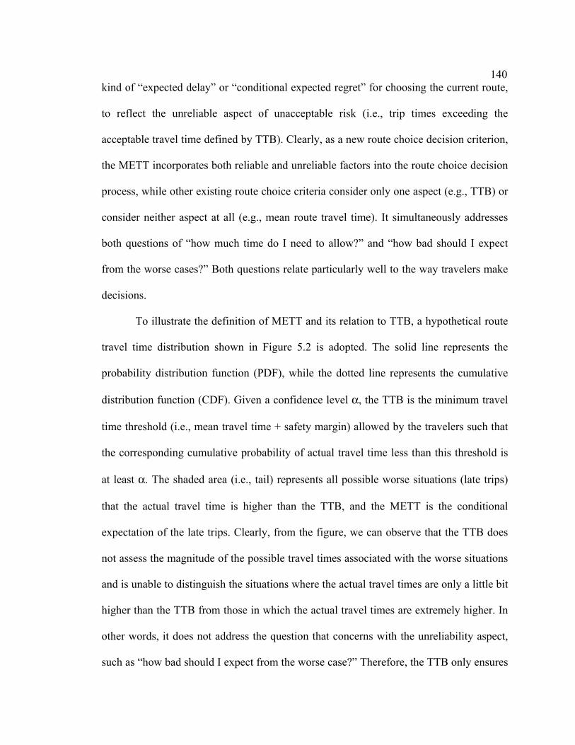
140kind of “expected delay” or “conditional expected regret” for choosing the current route,

to reflect the unreliable aspect of unacceptable risk (i.e., trip times exceeding the

acceptable travel time defined by TTB). Clearly, as a new route choice decision criterion,

the METT incorporates both reliable and unreliable factors into the route choice decision

process, while other existing route choice criteria consider only one aspect (e.g., TTB) or

consider neither aspect at all (e.g., mean route travel time). It simultaneously addresses

both questions of “how much time do I need to allow?” and “how bad should I expect

from the worse cases?” Both questions relate particularly well to the way travelers make

decisions.

To illustrate the definition of METT and its relation to TTB, a hypothetical route

travel time distribution shown in Figure 5.2 is adopted. The solid line represents the

probability distribution function (PDF), while the dotted line represents the cumulative

distribution function (CDF). Given a confidence level α, the TTB is the minimum travel

time threshold (i.e., mean travel time + safety margin) allowed by the travelers such that

the corresponding cumulative probability of actual travel time less than this threshold is

at least α. The shaded area (i.e., tail) represents all possible worse situations (late trips)

that the actual travel time is higher than the TTB, and the METT is the conditional

expectation of the late trips. Clearly, from the figure, we can observe that the TTB does

not assess the magnitude of the possible travel times associated with the worse situations

and is unable to distinguish the situations where the actual travel times are only a little bit

higher than the TTB from those in which the actual travel times are extremely higher. In

other words, it does not address the question that concerns with the unreliability aspect,

such as “how bad should I expect from the worse case?” Therefore, the TTB only ensures

141the reliability aspect of on-time arrival for a given confidence level α, while the METT

accounts for both the reliability aspect (i.e., TTB required to ensure on-time arrival at a

confidence level α) and the unreliability aspect of travel time variability (i.e.,

encountering worse travel times beyond the TTB in the tail).

Illustrative example

The following illustrative example shows the differences of using the expected

travel time, TTB, and METT as the route choice criterion. A small hypothetical network

with three parallel routes connecting origin r and destination s is adopted in this

demonstration (see Figure 5.3). In this example, all travelers are assumed to have a

confidence level of α = 90%. In order to facilitate the presentation of the essential ideas,

the travel time distributions of the three routes are assumed to follow a log-normal

distribution ( ),Logn µ σ , whose PDF is shown as below:

0 5 10 15 20 25 30

P r o

b a

b i

l i t

y D

e n

s i

t y

0 5 10 15 20 25 300

0.1

0.2

0.3

0.4

0.5

0.6

0.7

0.8

0.9

1

R o u t e T r a v e l T i m e

T r

a v

e l

T i

m e

R e

l i a

b i

l i t

y

C u m u l a t i v e P r o b a b i l i t y

P r o b a b i l i t y D e n s i t y

C o n f i d e n c e L e v e l

T r a v e l T i m e B u d g e t

M e a n E x c e s s T r a v e l T i m e

Figure 5.2 Illustration of the travel time budget and mean-excess travel time.

142

( ) ( )2

2

ln1| , exp22

fξ µ

ξ µ σσξσ π

⎛ ⎞− −= ⎜ ⎟

⎜ ⎟⎝ ⎠

, 0ξ∀ > . (5.6)

The log-normal distribution is closely related to the normal distribution and has

been commonly adopted in practice to model a broad range of random processes. The

parameters µp and σp of the log-normal distribution ( ),Logn µ σ for each route p (p = 1, 2,

3) are shown in Figure 5.3.

In this simple network where the route is equal to the link, the solution for the

expected travel time criterion can be derived analytically as follows.

( ) ( )2exp 2pppp TE σµπ +== , (5.7)

where Tp represents the random travel time of route p (p = 1, 2, 3).

If the travelers are concerned with travel time reliability and want to minimize

their corresponding TTB at the same time, the following minimization problem should be

considered (Chen and Ji, 2005):

( )minp

p p pE Tγ

ξ γ= + (5.8)

Figure 5.3 Hypothetical network used to illustrate the different route choice criteria.

143 s.t. ( )Pr 90%p pT ξ≤ ≥ . (5.9)

Under the assumption of the log-normal distributed route travel time, the TTB for

each route can be analytically computed (Aitchison and Brown, 1957) as follows:

( )( )1exp 2 2 1p p perfξ σ α µ−= − + , (5.10)

where ( )1erf − ⋅ is the inverse of the Gauss error function defined as:

( ) ( )2

0

2 expx

erf x t dtπ

= −∫ . (5.11)

Now, suppose travelers are concerned with not only the reliability of on-time

arrival, but also the impact of situations that actual travel times are higher than the TTB.

Then, it is meaningful for them to minimize the METT, while still ensures the reliability

requirement. Following the METT definition in Eq. (5.1), we consider the following

minimization problem:

min [ | ]p p p pE T Tη ξ= ≥ (5.12)

s.t. ( )Pr 90%p pT ξ≤ ≥ . (5.13)

Under the assumption of lognormal distribution, the minimization problem (5.12)

and (5.13) can be rewritten as:

( )

( )2

2

ln1 1min exp1 0.9 22p

p pp p

pp p

TT dT

Tξ

µσπ σ

∞⎛ ⎞− −⎜ ⎟⋅⎜ ⎟− ⋅⎝ ⎠

∫ (5.14)

( ). . Pr 90%p ps t T ξ≤ ≥ . (5.15)

By performing some calculus manipulations on the minimization problem (5.14)

and (5.15), the METT of route p can be analytically derived as follows:

144

( )2

20

ln1 1 exp1 22

p pp p p p p

pp p

TT dT

T

µη ξ ξ

α σπ σ∞ +

⎛ ⎞− −⎜ ⎟⎡ ⎤= + − ⋅⎣ ⎦ ⎜ ⎟− ⋅⎝ ⎠

∫

( ) ( )( )2 1exp 2 2 2 1p p perfµ σ α σ−= + ⋅Φ − ⋅ − + , (5.16)

where ( )Φ ⋅ is the standard normal CDF, [ ]a a+ = if 0a > , and [ ] 0a + = otherwise.

The analytically derived results for all three routes are shown in Figure 5.4, where

the x-axis represents the different route choice criteria and the z-axis represents the

corresponding measurement value (in minutes) for a given criterion. For simplicity, the

mean travel time, travel time budget and mean-excess travel time are abbreviated by

MTT, TTB and METT, respectively.

From Figure 5.4, it is clear that different route choice criteria provide different

optimal routes, which reflect various risk preferences and considerations of the travelers

toward travel time variability. If the travelers are all risk-neutral, they only consider the

expected route travel time during their route choice decisions (i.e., the traditional UE

model). Therefore, based on the first group of bars in the figure, they should choose route

3, which has the minimum expected travel time of 7. However, to ensure a 90%

confidence level of on-time arrival, choosing route 3 will no longer be the optimal

decision. If the travelers are risk-averse and concern more about the travel time reliability,

they may choose a route that gives them the minimum TTB. This can be observed in

Figure 5.5, where the TTB for each route is represented by the summation of two parts,

i.e., mean travel time plus an extra buffer time. This is consistent with the definition of

TTB given in Eq. (5.3), where the buffer time describes the impacts from the reliability

aspect of travel time variability on travelers’ route choice decisions. From the figure, we

145

MTT

TTB

METT

0

4

8

12

16

18

M i

n u

t e s

R o u t e 1R o u t e 2R o u t e 3

10

7

8

13.9314.80

17.08

12.1712.51

12.64

Figure 5.4 Analytical results for all three routes with different route choice criteria. can see that to make sure a 90% travel time reliability, route 3 has to add the longest

buffer time (5.51 min), which makes its TTB higher than that of route 2. Therefore, by

considering the impacts of the travel time reliability aspect, travelers will prefer route 2

due to its lowest TTB. In other words, travelers who plan to travel through route 2 may

depart later than those who choose other routes and still ensure a 90% confidence level of

punctual arrival.

However, as discussed in the previous section, TTB is unable to account for the

magnitude of the worse travel times in the distribution tail. That is, it is unable to assess

the impacts related to the unreliable situations where the actual travel times may be

146

0

5

10

15

Route 1

Route 2

Route 3

Buffer Time+

MTT=

TTB

M i n u t e s

5.51

7

4.17

812.51

12.17

12.64

10

2.64

Figure 5.5 Analysis of the impacts of travel time reliability. overwhelmingly higher than the TTB. Therefore, routes with a lower TTB may have a

higher METT, and travelers who choose these routes will have a 10% probability of

encountering trip times much greater than the allowable TTB. This can be demonstrated

more clearly in Figure 5.6, where the METT for each route is represented by the

summation of three parts, i.e., mean travel time, buffer time and “expected delay.” This is

consistent with the definition of METT by combining Eq. (5.3) and Eq. (5.5) , where the

“expected delay” describes the impacts from the unreliability aspect of travel time

variability on travelers’ route choice decisions, and the summation of the other two

components (mean travel time and buffer time) give the TTB that represents the travel

time reliability requirement specified by the travelers.

From the figure, we can see that travelers on route 2 or 3 may experience a higher

expected delay than those on route 1 when the 10% worse cases happened, even though

they has a lower TTB. These worse cases may be due to various sources, such as severe

147

05

1015

20

Route 1

Route 2

Route 3

4.57

5.51

7

2.63

1.29 2.64

10

817.08

13.93

14.80

+ExpectedDelay Buffer

Time +MTT

=METT

4.17

M i n u t e s

Figure 5.6 Analysis of the impacts of travel time unreliability. incidents, bad weather conditions and special events. Therefore, for travelers who are

concerned with not only the travel time reliability, but also the unreliability of

encountering worse travel times, they may prefer to choose route 1, which has the lowest

METT. Though, by doing that, the corresponding TTB is not the minimum, the

expectation of the unacceptable travel times greater than the allowable TTB is

significantly reduced compared to other choices. In addition, they can still enjoy at least a

90% reliability of punctual arrival. Note that the METT is always higher than the

corresponding TTB. This implies that the METT criterion can be regarded as a more

conservative measure of risk, which reflects the behavior of travelers who have a more

negative attitude toward schedule delay and a higher degree of risk-averseness in hedging

against travel time variability. The impacts on travelers’ route choice decision by

148considering both travel time reliability and unreliability can be further illustrated in

Figure 5.7 to show the percentages of each component (i.e., mean travel time, buffer time

and expected delay) corresponding to the METTs. From the figure, we can see that the

unreliability aspect of travel time variability is as significant as the reliability aspect on

travelers’ route choice decision. For example, the buffer time (reliability aspect) and the

expected delay (unreliability aspect) of route 3 are 32% and 27% of METT, respectively.

Furthermore, we can see that the reliability and unreliability aspects on route 3 have

nearly 59% impacts in total on travelers’ route choice decisions, which even higher than

the impacts from the mean travel time (only around 41%). It demonstrates that the

reliability and unreliability aspects do play an important role in travelers’ route choice

decisions under travel time variability. Therefore, none of them (reliability and

unreliability aspects) should be ignored in practice.

Equilibrium conditions and variational inequality formulation Consider a strongly connected transportation network [N, A], where N and A denote the

19%

72%

9%

28%

18%

54% 32%

27%

41%

BufferTime

ExpectedDelay

ExpectedDelay

ExpectedDelay

MTT

MTTMTT

BufferTime

Buffer Time

Route 1 Route 2 Route 3

Figure 5.7 Proportion of each component in the mean-excess travel times.

149

sets of nodes and links, respectively. Let R and S denote a subset of N for which travel

demand rsq is generated from origin r R∈ to destination s S∈ , and let rspf denote the

flow on route rsp P∈ , where rsP is a set of routes from origin r to destination s. We

assume that the link travel time is stochastic, which is represented by a random vector

aT T= , where aT represents the random travel time on link a A∈ .

Let rspaδ⎡ ⎤∆ = ⎣ ⎦ denote the route-link incidence matrix, where 1rs

paδ = if route p

from origin r to destination s uses link a, and 0, otherwise. Then, the feasible flow set Ω

can be described as below:

, ,rs

rs rsp

p P

q f r R s S∈

= ∀ ∈ ∈∑ , (5.17)

,rs

rs rsa p pa

r R s S p P

v f a Aδ∈ ∈ ∈

= ∀ ∈∑∑ ∑ , (5.18)

0, , ,rs rspf p P r R s S≥ ∀ ∈ ∈ ∈ , (5.19)

where (5.17) is the travel demand conservation constraint, (5.18) is a definitional

constraint that sums up all route flows that pass through a given link a, and (5.19) is a

non-negativity constraint on the route flows.

As discussed in the previous section, it is reasonable to assume that travelers are

willing to minimize their METT when traveling from an origin to a destination under an

uncertain environment. Consequently, a long-term habitual traffic equilibrium can be

reached. It is termed the mean-excess traffic equilibrium model. Let η denote the METT

vector ( ), ,Trs

pη… … , rsπ denote the minimal METT between O-D pair (r,s), and f denote

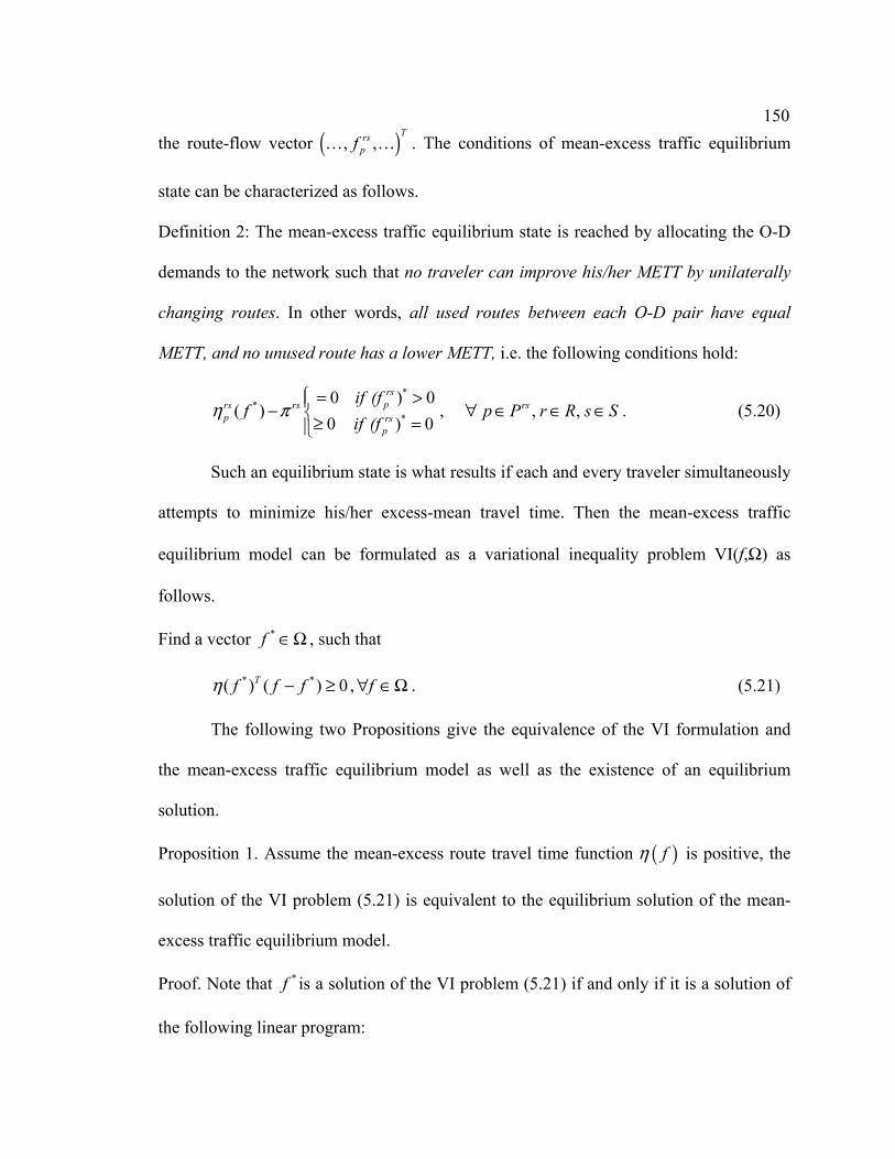
150the route-flow vector ( ), ,

Trspf… … . The conditions of mean-excess traffic equilibrium

state can be characterized as follows.

Definition 2: The mean-excess traffic equilibrium state is reached by allocating the O-D

demands to the network such that no traveler can improve his/her METT by unilaterally

changing routes. In other words, all used routes between each O-D pair have equal

METT, and no unused route has a lower METT, i.e. the following conditions hold:

*

**

0 ) 0( ) , , ,

0 ) 0

rsprs rs rs

p rsp

if (ff p P r R s S

if (f η π

⎧ = >⎪− ∀ ∈ ∈ ∈⎨≥ =⎪⎩. (5.20)

Such an equilibrium state is what results if each and every traveler simultaneously

attempts to minimize his/her excess-mean travel time. Then the mean-excess traffic

equilibrium model can be formulated as a variational inequality problem VI(f,Ω) as

follows.

Find a vector *f ∈Ω , such that

* *( ) ( ) 0Tf f fη − ≥ , f∀ ∈Ω . (5.21)

The following two Propositions give the equivalence of the VI formulation and

the mean-excess traffic equilibrium model as well as the existence of an equilibrium

solution.

Proposition 1. Assume the mean-excess route travel time function ( )fη is positive, the

solution of the VI problem (5.21) is equivalent to the equilibrium solution of the mean-

excess traffic equilibrium model.

Proof. Note that *f is a solution of the VI problem (5.21) if and only if it is a solution of

the following linear program:

151 ( )*min

T

ff fη

∈Ω (5.22)

By considering the primal-dual optimality conditions of (5.22), we have

( )* *( ) 0, , ,rs rs rs rsp pf f p P r R s Sη π⋅ − = ∀ ∈ ∈ ∈ , (5.23)

*( ) 0, , ,rs rs rsp f p P r R s Sη π− ≥ ∀ ∈ ∈ ∈ , (5.24)

and Eq. (5.19). It is easy to see the METE condition (5.20) is satisfied. This completes

the proof. €

Proposition 2. Assume the mean-excess route travel time function ( )fη is positive and

continuous, the mean-excess traffic equilibrium problem has at least one solution.

Proof. According to Proposition 1, we only need to consider the equivalent VI

formulation. Note that the feasible set Ω is nonempty and convex. Furthermore, the

mapping ( )fη is continuous according to the assumption. Thus, the VI problem (5.21)

has at least one solution (e.g., see Nagurney, 1993). This completes the proof. €

Note that, in this study, the travelers are assumed to be risk-averse and concerned

with both reliability and unreliability aspects of travel time variability, where the link

travel time distribution is assumed to has a continuous CDF by fitting the real

surveillance data. Consider the link/route relationship

, , ,rs rs rsp a ap

a AT T p P r R s Sδ

∈

= ∀ ∈ ∈ ∈∑ (5.25)

and the definition of the METT in Eq. (5.1), it is reasonable to give the positive and

continuous assumption of the function ( )fη as in the above propositions. Consequently,

the validity of the VI formulation and the existence of the solution are ensured.

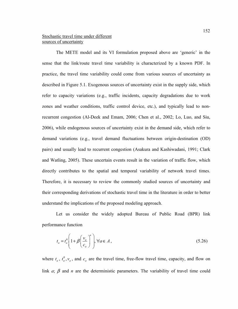
152Stochastic travel time under different sources of uncertainty

The METE model and its VI formulation proposed above are ‘generic’ in the

sense that the link/route travel time variability is characterized by a known PDF. In

practice, the travel time variability could come from various sources of uncertainty as

described in Figure 5.1. Exogenous sources of uncertainty exist in the supply side, which

refer to capacity variations (e.g., traffic incidents, capacity degradations due to work

zones and weather conditions, traffic control device, etc.), and typically lead to non-

recurrent congestion (Al-Deek and Emam, 2006; Chen et al., 2002; Lo, Luo, and Siu,

2006), while endogenous sources of uncertainty exist in the demand side, which refer to

demand variations (e.g., travel demand fluctuations between origin-destination (OD)

pairs) and usually lead to recurrent congestion (Asakura and Kashiwadani, 1991; Clark

and Watling, 2005). These uncertain events result in the variation of traffic flow, which

directly contributes to the spatial and temporal variability of network travel times.

Therefore, it is necessary to review the commonly studied sources of uncertainty and

their corresponding derivations of stochastic travel time in the literature in order to better

understand the implications of the proposed modeling approach.

Let us consider the widely adopted Bureau of Public Road (BPR) link

performance function

0 1 ,n

aa a

a

vt t a Ac

β⎛ ⎞⎛ ⎞⎜ ⎟= + ∀ ∈⎜ ⎟⎜ ⎟⎝ ⎠⎝ ⎠

, (5.26)

where at , 0at , av , and ac are the travel time, free-flow travel time, capacity, and flow on

link a; β and n are the deterministic parameters. The variability of travel time could

153come from the free-flow travel time, the link flow, or the link capacity as described

below.

Free-flow travel time variation. To describe the travel time variability due to

various non-routine events such as weather, road conditions, or traffic delays,

Mirchandani and Soroush (1987) suggested a nonnegative random free-flow link travel

time 0aT , which follows a Gamma distribution with shape parameter k and scale

parameter θ, i.e., ( )0 ,aT k θΓ∼ . Then, the mean and variance of aT can be represented as

below:

( ) 1n

aa

a

vE T kc

θ β⎛ ⎞⎛ ⎞⎜ ⎟= + ⎜ ⎟⎜ ⎟⎝ ⎠⎝ ⎠

, (5.27)

( )2

2 1n

aa

a

vVar T kc

θ β⎛ ⎞⎛ ⎞⎜ ⎟= + ⎜ ⎟⎜ ⎟⎝ ⎠⎝ ⎠

. (5.28)

Capacity variation. Lo, Luo, and Siu (2006) considered stochastic link capacity

degradation, which is one of the main sources of travel time variability. Under the

relatively minor day-to-day events, such as vehicle breakdown and accident, the link

capacity is subject to stochastic degradation to different degrees. By assuming the

capacity degradation random variable aC (we use capital letters to represent random

variables) is independent of the amount of traffic ( av ) on it, and follows a uniform

distribution defined by an upper bound (the design capacity ac ) and a lower bound (the

worst-degraded capacity, to be a fraction aρ of the design capacity), Lo, Luo, and Siu,

(2006) derived the mean and variance of aT as below:

154

( ) ( )( )( )

10 0

11 1

nan

a a a a na a

E T t t vc n

ρβ

ρ

−−= +

− −, (5.29)

( ) ( ) ( )( ) ( )( )

21 2 122 0 22

1 11 1 2 1 1

n nn a a

a a a n na a a a

Var T t vc n c n

ρ ρβρ ρ

− −⎧ ⎫⎡ ⎤− −⎪ ⎪= −⎨ ⎬⎢ ⎥− − − −⎣ ⎦⎪ ⎪⎩ ⎭. (5.30)

To relax the assumption of uniform distribution, they suggested adopting the

Mellin Transform technique as discussed in Lo and Tung (2003).

Demand variation. Another main source of travel time variability is the stochastic

travel demand. In view of the day-to-day travel demand fluctuation, the traffic demand

between each OD pair is assumed to be a random variable with a given probability

distribution:

, ,rs rs rsQ q r R s Sε= + ∀ ∈ ∈ , (5.31)

where ( )rs rsq E Q= is the mean demand, and rsε is the random term with ( ) 0rsE ε = .

Consequently, the route flow rspF and link flow aV are also random variables that

contribute to travel time variability. By assuming that the route flow follows the same

type of probability distribution as the OD demand, the route flow’s coefficient of

variation (CV) is equal to that of the OD demand, and the route flows are mutually

independent, Shao et al. (2006) analytically derived the mean and variance of aT based on

the assumption that the OD demands are normally distributed (Asakura and Kashiwadani,

1991; Clark and Watling, 2005) as follows.

[ ]( )

( ) ( ) ( )0

0

0,

1 !!,n i n iva

a a a ani i evena

ntE T t v i a Aic

β σ −

= =

⎛ ⎞= + − ∀ ∈⎜ ⎟

⎝ ⎠∑ , (5.32)

155

[ ]( )

( ) ( ) ( )

( ) ( ) ( )

20 2

2

0,

2

0,

21 !!

1 !! ,

n i n ivaa a an

i i evena

n i n iva a

i i even

ntVar T v iic

nv i a A

i

β σ

σ

−

= =

−

= =

⎛ ⎞ ⎛ ⎛ ⎞= −⎜ ⎟ ⎜ ⎜ ⎟⎜ ⎟ ⎝ ⎠⎝⎝ ⎠

⎞⎛ ⎞⎛ ⎞ ⎟− − ∀ ∈⎜ ⎟⎜ ⎟ ⎟⎝ ⎠⎝ ⎠ ⎠

∑

∑, (5.33)

where ( )1 !!i − is the double factorial of 1i − , i.e., ( ) ( )( )1 !! 1 3 2i i i− = − − … ( i is even),

ni

⎛ ⎞⎜ ⎟⎝ ⎠

is binomial coefficient, i.e., ( )

!! !

n ni n i i

⎛ ⎞=⎜ ⎟ −⎝ ⎠

, and vaσ is the standard deviation of the

random link flow.

Under similar assumptions, except that the route flow’s variance-to-mean ratio

(VMR) is assumed to be equal to that of the OD demand to maintain the flow

conservation constraints, Zhou and Chen (Chapter 6) analytically derived the mean and

variance of aT based on the log-normal distribution as follows.

[ ]( )22

00 2

vav

a

nna

a a na

tE T t eC

σµβ +

⎛ ⎞⎜ ⎟= +⎜ ⎟⎜ ⎟⎝ ⎠

, a A∀ ∈ , (5.34)

[ ] ( ) ( )2 22 220

21( )

v v va a an n na

a na

tVar T e eC

σ µ σβ +⎛ ⎞ ⎡ ⎤= − ⋅⎜ ⎟ ⎢ ⎥⎣ ⎦⎝ ⎠, a A∀ ∈ . (5.35)

where vaµ and v

aσ are the parameters of the link flow distribution ( ),v va aLogn µ σ .

It should be noted that the assumption of mutually independent route flows can

also be relaxed (Luathep, Sumalee, and Lam, 2007; Shao, 2007).

Recently, some researches (Shao et al., 2008; Siu and Lo, 2008) were conducted

to model travelers’ route choice behavior under travel time variability due to both

demand fluctuation and link capacity degradation. Shao et al. (2008) considered the rain

156effects on road network, where the link free-flow travel time is represented by a non-

decreasing function of rainfall intensity, the link capacity is represented by a non-

increasing function of rainfall intensity, and travel demand is stochastic. Siu and Lo

(2008) considered the travel demand is composed of two parts: commuters and non-

commuters, where the randomness of travel demand is assumed to be introduced by the

volume of non-commuters, and the link capacity is subject to stochastic degradation.

Derivation of METT. To facilitate the presentation of the essential ideas, we

assume that the link travel times are independent. This assumption is also adopted by Lo,

Luo, and Siu (2006); Shao et al. (2006), Siu and Lo (2006), and Watling (2006). Hence,

the mean and variance of rspT can be written as:

[ ] , , ,rs rs rs rsp p a pa

a A

E T E T p P r R s Sµ δ∈

⎡ ⎤= = ∀ ∈ ∈ ∈⎣ ⎦ ∑ , (5.36)

( ) [ ]2, , ,rs rs rs rs

p p a paa A

Var T Var T p P r R s Sσ δ∈

⎡ ⎤= = ∀ ∈ ∈ ∈⎣ ⎦ ∑ . (5.37)

According to the Central Limit Theorem, for routes consisting of many links, the

random route travel times tend to be normal distributed regardless of what the underlying

link travel time distribution is (Lo and Tung, 2003; Shao et al., 2006):

( )( )2~ ,rs rs rs

p p pT N µ σ . (5.38)

Then, according to the definition of the METT in Eq. (5.1) and assuming the

travelers’ confidence level is α, the route METT can be represented as the following

minimization problem:

157

( )

( )( )

( )2

21 1min exp

1 2 2rsp

rs rsp prs rs

p prs rsp p

TT d T

ξ

µα πσ σ

∞⎛ ⎞−⎜ ⎟⋅ −⎜ ⎟−⎝ ⎠

∫ (5.39)

s.t. ( )

( )( )

2

21 exp

2 2

rsp

rs rsp p rs

prs rsp p

Td T

ξ µα

πσ σ∞

⎛ ⎞−⎜ ⎟− ≥⎜ ⎟⎝ ⎠

∫－ . (5.40)

Following some simple calculus manipulations, the METT of route p can be

represented as

( )

( )( )21

exp22 1

rsprs rs

p p

αση µ

π α

−⎛ ⎞Φ⎜ ⎟= + −⎜ ⎟−⎝ ⎠

. (5.41)

Note that, in reality, the link travel times may not be totally independent due to

the network topology or the sources of variations. Therefore, the effects of the covariance

of link travel times should be considered in future research. A recent attempt in this

direction can be found in Lam, Shao, and Sumalee (2008).

Other forms of travel time distributions were also proposed in the literature. For

example, exponential and uniform travel time distributions were adopted in Noland and

Small (1995) for studying the morning commute problem. A family of distributions

known as the “Johnson curves” was studied by Clark and Watling (2005) to model the

total network travel time under random demand. Gamma type distributions were tested

by Fan and Nie (2006) in the stochastic optimal routing problem. To allow for a more

flexible control over the right-hand tail and better fit the data, a mixture of normal

distribution was suggested in Watling (2006). However, no matter what kind of

distribution is assumed, the concept of METT and the METE model are still valid. METT

is a simple, convenient representation of risk, which fits quite well to the way that

158travelers' assess the reliability and unreliability aspects of travel time variability and

make their route choice decisions to tradeoff the buffer time measure (i.e., the reliability

aspect measured by TTB) and the tardy time measure (i.e., the unreliability aspect that

measures the worst travel times beyond TTB) accordingly.

Solution Procedure

A basic assumption of the traditional traffic equilibrium models is the additivity,

i.e. the route cost is simply the sum of the costs on the links that constitute that route.

This additive assumption enables the application of a number of well-known algorithms

(e.g., the Frank-Wolfe algorithm), and the traffic equilibrium problem can be solved

without the need to store routes. This is a significant benefit when one needs to solve

large-scale network problems (Boyce, Ralevic-Dekic, and Bar-Gera, 2004). However,

these types of algorithms are not applicable to the METE model, since the METT is

nonadditive in general. Therefore, to solve the proposed model, a route-based algorithm

is needed (Bernstein and Gabriel, 1997; Chen Lo, and Yang, 2001; Gabriel and Bernstein,

1997; Lo and Chen, 2000).

Main ideas of the solution procedure. By exploring the special structure of the

METE model, a modified alternating direction (MAD) algorithm, which is a kind of

projection-based algorithm, is adopted in this study (Han, 2002) for solving the VI

problem (Eq. (5.21)). By attaching a Lagrangian multiplier vector y to the demand

conservation constraints Eq.(5.17), we can reformulate the METE model as an equivalent

VI problem, denoted as ( ),VI F K shown below:

159Find u K∗ ∈ , such that

* *( ) ( ) 0,TF u u u u K− ≥ ∀ ∈ , (5.42)

where

f

uy

⎛ ⎞= ⎜ ⎟⎝ ⎠

, ( )

( )Tf y

F uf q

η⎛ ⎞− Λ= ⎜ ⎟Λ −⎝ ⎠

, n kK R R+= × , (5.43)

where Λ denotes the OD-Route incidence matrix, q denotes the demand vector

( ), ,Trsq… … , n is the total number of routes, and k is the total number of OD pairs. Based

on this transformation, we can see that a projection on the new feasible region K is much

easier than on the original set Ω. Therefore, in each iteration, the MAD algorithm can

make a simple projection on the set K to update the solution vector u. This simple

projection makes the MAD algorithm very attractive. Furthermore, a self-adaptive

stepsize updating scheme is embedded in the MAD algorithm, where the stepsize is

automatically updated according to the information of the previous iterations (i.e., route

flows and route METT). These features make the MAD algorithm efficient and robust.

The global convergence of the MAD algorithm can be rigorously proven under mild

conditions, which only require the underlying mapping ( )fη to be continuous and

monotone. However, the monotonicity is hard to guarantee in practice. Hence,

convergence may not always ensure, especially for large-scale networks.

Flowchart of the MAD algorithm. Based on the discussions above, the detailed

steps of the MAD algorithm can be represented in the following flowchart (Figure 5.8).

For more details about the MAD algorithm, such as the derivation of the descent

160direction ( , )k

kd u β and the scaling factor ( , )kkuρ β , we refer to Han (2002) and Zhou,

Chen and Han (2007). In the numerical experiments, we specify the initial stepsize

Figure 5.8 Flowchart of the MAD algorithm.

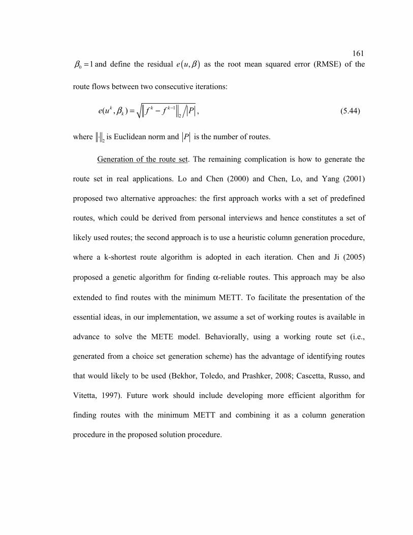
1610 1β = and define the residual ( ),e u β as the root mean squared error (RMSE) of the

route flows between two consecutive iterations:

1

2( , )k k k

ke u f f Pβ −= − , (5.44)

where 2

⋅ is Euclidean norm and P is the number of routes.

Generation of the route set. The remaining complication is how to generate the

route set in real applications. Lo and Chen (2000) and Chen, Lo, and Yang (2001)

proposed two alternative approaches: the first approach works with a set of predefined

routes, which could be derived from personal interviews and hence constitutes a set of

likely used routes; the second approach is to use a heuristic column generation procedure,

where a k-shortest route algorithm is adopted in each iteration. Chen and Ji (2005)

proposed a genetic algorithm for finding α-reliable routes. This approach may be also

extended to find routes with the minimum METT. To facilitate the presentation of the

essential ideas, in our implementation, we assume a set of working routes is available in

advance to solve the METE model. Behaviorally, using a working route set (i.e.,

generated from a choice set generation scheme) has the advantage of identifying routes

that would likely to be used (Bekhor, Toledo, and Prashker, 2008; Cascetta, Russo, and

Vitetta, 1997). Future work should include developing more efficient algorithm for

finding routes with the minimum METT and combining it as a column generation

procedure in the proposed solution procedure.

162Numerical Examples

To demonstrate the proposed METE model and solution procedure, two networks

are adopted in the numerical experiments. First, a small network is used to illustrate the

features of the proposed model, its differences compared to other traffic equilibrium

models, and the correctness of the solution procedure. Then, a medium-sized network is

employed to demonstrate the applicability of the solution procedure to larger networks.

Small network

To illustrate the proposed METE model, a simple network consists of 4 nodes, 5

links and 3 routes (Figure 5.9) is adopted, where the route-link relationship is shown in

Table 5.1. There is one OD pair (1, 4) with 1000 units of demand. The free-flow travel

time for each individual link is assumed to follow a normal distribution. The reason for

choosing a normal distribution in this numerical experiment is because it enables deriving

analytical expressions of the METT for each route. Therefore, we can solve the problem

analytically and use the results as a benchmark to compare the METE model with the

Figure 5.9 Small network.

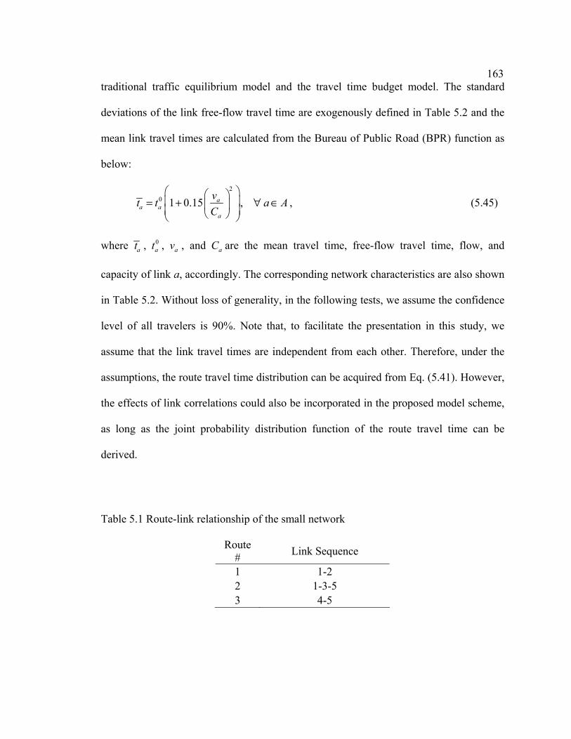
163traditional traffic equilibrium model and the travel time budget model. The standard

deviations of the link free-flow travel time are exogenously defined in Table 5.2 and the

mean link travel times are calculated from the Bureau of Public Road (BPR) function as

below:

2

0 1 0.15 ,aa a

a

vt t a AC

⎛ ⎞⎛ ⎞⎜ ⎟= + ∀ ∈⎜ ⎟⎜ ⎟⎝ ⎠⎝ ⎠

, (5.45)

where at , 0at , av , and aC are the mean travel time, free-flow travel time, flow, and

capacity of link a, accordingly. The corresponding network characteristics are also shown

in Table 5.2. Without loss of generality, in the following tests, we assume the confidence

level of all travelers is 90%. Note that, to facilitate the presentation in this study, we

assume that the link travel times are independent from each other. Therefore, under the

assumptions, the route travel time distribution can be acquired from Eq. (5.41). However,

the effects of link correlations could also be incorporated in the proposed model scheme,

as long as the joint probability distribution function of the route travel time can be

derived.

Table 5.1 Route-link relationship of the small network

Route # Link Sequence

1 1-2 2 1-3-5 3 4-5

164The equilibrium route flow pattern is shown in Table 5.3, as well as the

corresponding mean travel time, TTB and METT. To check the validity of the results, we

examine two conditions: travel demand conservation constraints and METE equilibrium

conditions. As expected, all conditions are satisfied. The route flows sum up to the OD

travel demands and the METT of all used routes are equal and minimal. Furthermore, to

analyze the impact of travel time variability on travelers’ route choice decisions, the

percentages of the three travel time components (mean travel time, buffer time, and

‘expected delay’) that compose the METT for each route are depicted in Figure 5.10. As

we discussed before, the summation of the mean travel time and the buffer time gives the

TTB, which represents the travel time reliability requirement of the travelers. Specifically,

in this experiment, the travelers are assumed to have a 90% confidence level of on-time

arrival. At the same time, the “expected delay” describes the unreliability aspect of travel

time variability, which evaluates the risk associated with the unacceptable late arrivals

(though infrequent) that have a travel time excessively higher than the TTB. From the

figure, we can see that the reliability and unreliability aspects of travel time variability

have around 15% - 20% impacts on travelers’ route choice decisions. Though the

Table 5.2 Network characteristics

Link # Free-flow travel time

( 0at ) Capacity (Ca)

Standard deviation of the free-flow travel time

1 5 600 2 2 12 400 6 3 7 400 1 4 10 400 5 5 8 600 2

165percentage of the impacts associated with the unreliability aspect is not high (around 5%)

in this simple example, which is due to the normally distributed link free-flow travel time,

it is expected to play a more significant role in the travelers’ route choice decisions under

highly skew link travel time distributions in practice.

In the following, we further compare the METE model with the conventional UE

model and the reliability-based user equilibrium model. Recall that the route choice

criterion in the conventional UE model is the mean route travel time, while the reliability-

based user equilibrium model adopts the concept of TTB. To simplify the notation, we

use UE and RUE to represent the conventional UE model and the reliability-based user

equilibrium model, respectively. Conceptually, the TTB model (Lo, Luo, and Siu, 2006)

and DRUE model (Shao et al., 2006) are all RUE model, since they all share the common

Table 5.3 Equilibrium results of the METE model Route # Route flow Mean travel time Travel time budget Mean-excess travel time

1 499.68 20.43 24.06 25.40 2 47.82 21.47 24.34 25.40 3 452.50 20.75 24.15 25.40

14%

80%

5%

85%

11%4%

82%

13%5%

MTT MTTMTT

Buffer TimeBuffer Time Buffer TimeExpectedDelay

ExpectedDelay

ExpectedDelay

Route 1 Route 2 Route 3

Figure 5.10 Analysis of the reliability and unreliability aspects of travel time variability

on travelers’ route choice decision.

166route choice criterion despite that the original sources of travel time variation are

different. The equilibrium results of the three models are demonstrated in Table 5.4 and

Figure 5.11 - Figure 5.13, where the x-axis represents different equilibrium models, the

y-axis represents the mean travel time, TTB and mean excess travel time of each route

under the equilibrium state of each individual model, respectively.

From the table and figures, it is clear that the three user equilibrium models give

quite different equilibrium flow patterns. In the following, we further investigate the

differences among these three models. First, we examine the results under the

conventional UE model (see Figure 5.11). In the equilibrium state, two used routes (route

1 and 3) with equal and minimum mean travel times have positive flows, while the

unused route (route 2) with a higher mean travel time carries no flow. However, as we

discussed above, the route choice model under the mean travel time cannot account for

the risk associated with the travel time variation. Therefore, it shows that, under the

equilibrium state of the conventional UE model, though route 2 has the highest mean

travel time, it actually has the second lowest TTB and the lowest mean excess travel time.

This is because the travel time variance of route 2 is the lowest among the all three routes.

Therefore, under the consideration of reliability aspects of travel time variability, the

travelers on route 1 are willing to switch to route 2 or 3. When more travelers shift to

Table 5.4 Equilibrium route flows of different user equilibrium models

Route # UE RUE METE 1 532.40 517.77 499.682 0.00 13.23 47.823 467.60 469.00 452.50

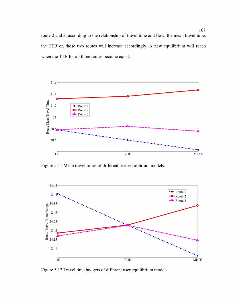
167route 2 and 3, according to the relationship of travel time and flow, the mean travel time,

the TTB on those two routes will increase accordingly. A new equilibrium will reach

when the TTB for all three routes become equal.

UE RUE METE

20.6

20.8

21

21.2

21.4

21.6

Rou

te M

ean

Trav

el T

ime

Route 1Route 2Route 3

Figure 5.11 Mean travel times of different user equilibrium models.

UE RUE METE

24.1

24.15

24.2

24.25

24.3

24.35

24.4

24.45

Rou

te T

rave

l Tim

e B

udge

t

Route 1Route 2Route 3

Figure 5.12 Travel time budgets of different user equilibrium models.

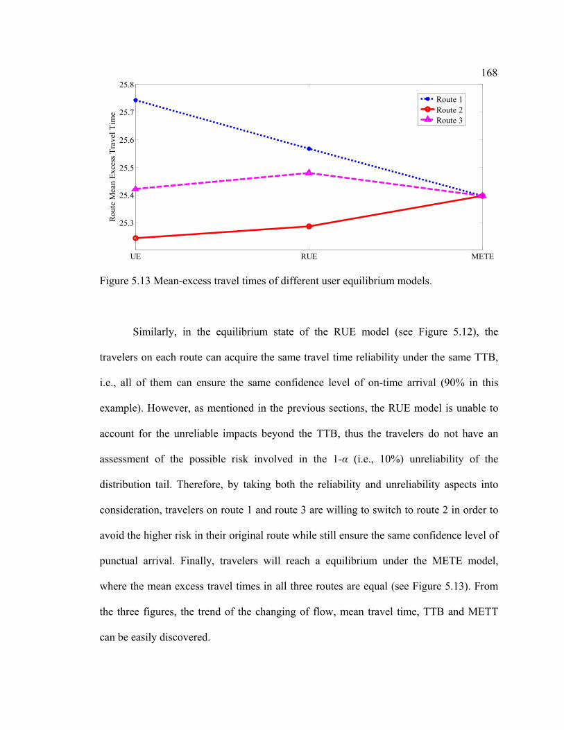
168

UE RUE METE

25.3

25.4

25.5

25.6

25.7

25.8

Rou

te M

ean

Exce

ss T

rave

l Tim

e

Route 1Route 2Route 3

Figure 5.13 Mean-excess travel times of different user equilibrium models.

Similarly, in the equilibrium state of the RUE model (see Figure 5.12), the

travelers on each route can acquire the same travel time reliability under the same TTB,

i.e., all of them can ensure the same confidence level of on-time arrival (90% in this

example). However, as mentioned in the previous sections, the RUE model is unable to

account for the unreliable impacts beyond the TTB, thus the travelers do not have an

assessment of the possible risk involved in the 1-α (i.e., 10%) unreliability of the

distribution tail. Therefore, by taking both the reliability and unreliability aspects into

consideration, travelers on route 1 and route 3 are willing to switch to route 2 in order to

avoid the higher risk in their original route while still ensure the same confidence level of

punctual arrival. Finally, travelers will reach a equilibrium under the METE model,

where the mean excess travel times in all three routes are equal (see Figure 5.13). From

the three figures, the trend of the changing of flow, mean travel time, TTB and METT

can be easily discovered.

169Medium-size network

In this section, the proposed model and solution procedure are demonstrated using

the Sioux Falls network (Leblanc, 1973), which is a medium-sized network with 24

nodes, 76 links, and 550 OD pairs (see Figure 5.14). The working route set of the

network are from Bekhor, Toledo, and Prashker (2008), where the routes are generated

by using a combination of the link elimination method (Azevedo et al., 1993) and the

penalty method (De La Barra, Perez, and Anez, 1993). The total number of routes is 3441,

the maximum number of routes generated for any OD pair is 13, and the average number

of routes is 6.3 per OD pair.

In this experiment, we assume the travel time variability comes from the day-to-

day travel demand fluctuations. Here, the stochastic travel demands are assumed to

follow a lognormal distribution, which is a nonnegative, asymmetrical distribution and

has been adopted in the literature as a more realistic approximation of the stochastic

travel demand to examine the uncertainty of the four-step travel demand forecasting

model (Zhao and Kockelman, 2002). The PDF of the lognormal distribution is given as

follows.

( )( )2

2ln21| ,

2

x

f x ex

µσµ σ

σ π

− −

= , 0x∀ > , (5.46)

where x is the random variable, µ and σ are the distribution parameters, and the

mean and variance are 22σµ += em and ( )2 22 1v e eµ σ σ+= − , respectively. Under some

commonly adopted assumptions, the distribution of the random route travel time can be

analytically derived (Chapter 6). For simplicity, the VMT of route flows are assumed to

be 0.3, the stopping criterion ε is set to be 5e-3, and the initial route flow for a given OD

170

Figure 5.14 Sioux Falls network. pair is set to be the OD demand divided by the number of routes connecting this OD.

Then, the route-based traffic assignment algorithm is tested on a personal computer with

2.4 G Pentium-IV processor and 768M RAM.

The MAD algorithm terminates after 70 iterations and the CPU time is 24.52

seconds. The convergence of the MAD algorithm in terms of the RMSE is shown in

Figure 5.15.

171

0 10 20 30 40 50 60 70

0.015

0.025

0.035

N u m b e r o f I t e r a t i o n s

R M

S E

Figure 5.15 Convergence curve of the MAD algorithm.

To further demonstrate the convergence of the proposed solution procedure,

without loss of generality, we examine two routes connecting OD pair (1, 10). The link

sequence of Route 1 and Route 2 are 2 – 6 – 9 – 13 – 25 and 2 – 6 – 10 – 32, respectively.

The evolution of the route flow and the route METT during the iteration process are

represented in Figure 5.16 and Figure 5.17.

From the figures, we can see that the algorithm quickly converges to the required

solution precision. The METE solution is achieved as the RMSE approaches zero after 70

iterations. At the same time, the METTs of used routes for a given OD pair are getting

closer to each other during the iteration process. Furthermore, it can be observed that the

fluctuation of the RMSE is more frequent and larger at the early iterations, and getting

smaller along with the iteration process. It demonstrates that the proposed algorithm has

the ability to reach a stable equilibrium solution.

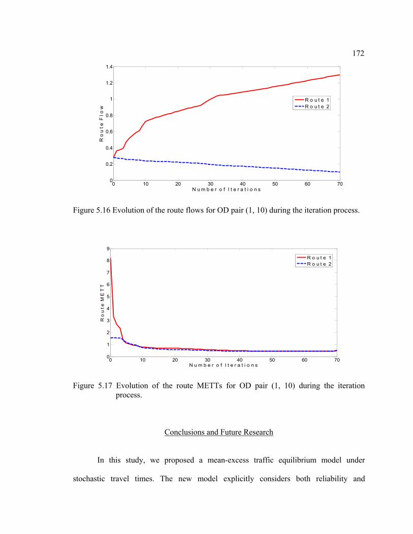
172

0 10 20 30 40 50 60 700

0.2

0.4

0.6

0.8

1

1.2

1.4

N u m b e r o f I t e r a t i o n s

R o

u t

e F

l o

w

R o u t e 1R o u t e 2

Figure 5.16 Evolution of the route flows for OD pair (1, 10) during the iteration process.

0 10 20 30 40 50 60 700

1

2

3

4

5

6

7

8

9

N u m b e r o f I t e r a t i o n s

R o

u t

e M

E T

T

R o u t e 1R o u t e 2

Figure 5.17 Evolution of the route METTs for OD pair (1, 10) during the iteration

process.

Conclusions and Future Research

In this study, we proposed a mean-excess traffic equilibrium model under

stochastic travel times. The new model explicitly considers both reliability and

173unreliability aspects of travel time variability in the travelers’ route choice decision

process. The new model is formulated as a variational inequality (VI) problem.

Qualitative properties, such as equivalence and existence of the solution, were also

rigorously proved. A route-based traffic assignment algorithm based on the modified

alternating direction method was adopted to solve the proposed model. Numerical

examples are also provided to highlight the essential ideas of the model and the to

demonstrate the proposed algorithm.

Many further works are worthy of exploring based on the proposed METE model.

In the computational point of view, more efficient algorithms for finding the nonadditive

METT routes and solving the proposed model need to be developed and tested on larger-

scale networks. From the behavioral aspect, empirical studies need to be performed to

obtain a better understanding of the travelers' risk preference and attitudes to travel time

variation. Furthermore, in this study, the travelers were assumed to have perfect

knowledge about the travel time distribution. This assumption could be relaxed by

incorporating a perception error in the METT of each route. Thus, during the equilibrium

process, travelers try to minimize their perceived METT, which is then corresponding to

an SUE counterpart to the METE model. Note that, in reality, different user classes may

have different attitudes towards risk or perception differences when making their route

choice decisions. Therefore, further extensions could be to incorporate multiple user

classes corresponding to traveler’s different risk preferences or perception errors into the

model.

Finally, by incorporating the specific sources of travel time variation, such as link

capacity degradation and traffic control devices, into the consideration of the proposed

174modeling approach, the METE model can be regarded as a fundamental component of

high level transportation system risk assessment framework. That is, the proposed model

can be extended for network design problem (NDP), where the functions of the METT

(e.g., total mean travel time of the whole network or OD mean travel time between

specific OD pairs) as system risk measures are to be minimized or act as constraints by

optimally determining the design variables subject to a budgetary constraint. To design a

more reliable/robust network by developing appropriate risk assessment measure and

efficient solution algorithm remains an important and active research topic in the future.

References

Abdel-Aty, M., R. Kitamura, and P. Jovanis. 1995. Exploring route choice behavior using

geographical information system-based alternative paths and hypothetical travel time information input. Transportation Research Record 1493: 74-80.

Aitchison, J., and J. A. C. Brown. 1957. The lognormal distribution with special

reference to its uses in econometrics, Cambridge University Press, Cambridge, U.K. 194 p.

Al-Deek, H., and E. B. Emam. 2006. New methodology for estimating reliability in

transportation networks with degraded link capacities. Journal of Intelligent Transportation Systems 10(3): 117-129.

Artzner, P., F. Delbaen, J. M. Eber, and D. Heath. 1997. Thinking coherently. Risk

10(11): 68-71. Artzner, P., F. Delbaen, J. M. Eber, and D. Heath 1999. Coherent measures of risk.

Mathematical Finance 9: 203-228. Asakura, Y., and M. Kashiwadani. 1991. Road network reliability caused by daily

fluctuation of traffic flow. European Transport, Highways & Planning 19: 73-84. Azevedo, J. A., M. E. O. Santos Costa, J. J. E. R. Silvestre Madera, and E. Q. Vieira

Martins. 1993. An Algorithm for the Ranking of Shortest Paths. European Journal of Operational Research 69: 97-106.

175Bekhor, S., T. Toledo, and J. N. Prashker. 2008. Effects of choice set size and route

choice models on path-based traffic assignment. Transportmetrica 4(2): 117-133. Bell, M. G. H. 2000. A game theory approach to measuring the performance reliability of

transport networks. Transportation Research Part B 34: 533-546. Bell, M. G. H., and C. Cassir. 2002. Risk-averse user equilibrium traffic assignment: An

application of game theory. Transportation Research Part B 36: 671-681. Bernstein, D., and S. A. Gabriel. 1997 Solving the nonadditive traffic equilibrium

problem, p. 72-102. Proceedings of the Network Optimization Conference, New York.

Boyce, D., B. Ralevic-Dekic, and H. Bar-Gera. 2004. Convergence of traffic assignments:

How much is enough? Journal of transportation engineering 130(1): 49-55. Brownstone, D., A. Ghosh, T. F. Golob, C. Kazimi, and D. V. Amelsfort. 2003. Drivers'

willingness-to-pay to reduce travel time: Evidence from the San Diego I-15 congestion pricing project. Transportation Research Part A 37(4): 373-387.

Cambridge Systematics, Inc., Texas Transportation Institute, University of Washington,

Dowling Associates. 2003. Providing a highway system with reliable travel times. NCHRP Report No. 20-58[3], Transportation Research Board, National Research Council, U.S.A.

Cascetta, E., F. Russo, and A. Vitetta. 1997. Stochastic user equilibrium assignment with

explicit path enumeration: Comparison of models and algorithms, p. 1078-1084. Proceedings of the International Federation of Automatic Control: Transportation systems, Chania, Greece.

Chen, A., and Z. Ji. 2005. Path finding under uncertainty. Journal of Advanced

Transportation 39(1): 19-37. Chen, A., H. K. Lo, and H. Yang. 2001. A self-adaptive projection and contraction

algorithm for the traffic assignment problem with path-specific costs. European Journal of Operational Research 135: 27-41.

Chen, A., H. Yang, H. K. Lo, and W. H. Tang. 2002. Capacity reliability of a road

network: An assessment methodology and numerical results. Transportation Research Part B. 36: 225-252.

Chen, G., M. S. Daskin, Z. J. M. Shen, and S. Uryasev. 2006. The alpha-reliable mean-

excess regret model for stochastic facility location modeling. Naval Research Logistics 53: 617-626.

176Clark, S. D., and D. Watling. 2005. Modelling network travel time reliability under

stochastic demand. Transportation Research Part B 39(2): 119-140. De La Barra, T. B. Perez, and J. Anez. 1993. Multidimensional Path Search and

Assignment, p. 307-319. Proceedings of the Proceedings of the 21st PTRC Summer Annual Meeting, Manchester, England.

de Palma, A., and N. Picard. 2005. Route choice decision under travel time uncertainty.

Transportation Research Part A 39: 295-324. Emmerink, R. H. M., K. W. Axhausen, P. Nijkamp, and P. Rietveld. 1995. The potential

of information provision in a simulated road network with non-recurrent congestion. Transportation Research Part C 3: 293-309.

Fan, Y. Y., and Y. Nie. 2006. Optimal Routing for Maximizing the Travel Time

Reliability. Networks and Spatial Economics 6(3): 333-344. FWHA. 2004. Traffic congestion and reliability trends and advanced strategies for

congestion mitigation. http://ops.fhwa.dot.gov/congestion_report_04 FHWA. 2006. Travel time reliability: Making it there on time, all the time. Report No. 70,

Federal Highway Administration. Gabriel, S. A., and D. Bernstein. 1997. The traffic equilibrium problem with nonadditive

path costs. Transportation Science 31(4): 337-348. Han, D. 2002. A modified alternating direction method for variational inequality

problems. Applied Mathematics and Optimization 45: 63-74. Hall, R. W. 1993. Non-recurrent congestion: How big is the problem? Are traveler

information systems the solution? Transportation Research Part C 1: 89-103. Lam, T. 2000. The effect of variability of travel time on route and time-of-day choice.

Unpublished Ph.D. dissertation. University of California, Irvine, CA. 174 p. Lam, W. H. K., and K. S. Chan. 2005. Impact of road pricing on road network reliability.

Journal of Eastern Asia Society for Transportation Studies 6: 2060-2075. Lam, W. H. K., H. Shao, and A. Sumalee. 2008. Modeling impacts of adverse weather

conditions on a road network with uncertainties in demand and supply. Submitted to Transportation Research Part B.

Larsen, N., H. Mausser, and S. Uryasev. 2002. Algorithms for optimization of value-at-

risk. ISE Dept. University of Florida.

177Leblanc, L. J. 1973. Mathematical Programming Algorithms for Large-Scale Network

Equilibrium and Network Design Problems. Unpublished PhD thesis, Northwestern University, Evanston IL.

Liu, H., W. Recker, and A. Chen. 2004. Uncovering the contribution of travel time

reliability to dynamic route choice using real-time loop data. Transportation Research Part A 38: 435-453.

Lo, H. K., and A. Chen. 2000. Traffic equilibrium problem with route-specific costs:

Formulation and algorithms. Transportation Research Part B 34: 493-513. Lo, H. K., X. W. Luo, and B. W. Y. Siu. 2006. Degradable transport network: Travel

time budget of travelers with heterogeneous risk aversion. Transportation Research Part B 40: 792-806.

Lo, H. K., and Y. K. Tung. 2003. Network with degradable links: Capacity analysis and

design. Transportation Research Part B 37: 345-363. Luathep, P., A. Sumalee, and W. H. K. Lam. 2007. Robust transport network capacity

planning with demand uncertainty. working paper, Hong Kong Polytechnic University.

Mirchandani, P., and H. Soroush. 1987. Generalized traffic equilibrium with probabilistic

travel times and perceptions. Transportation Science 21: 133-152. Nagurney, A. 1993. Network Economics: A Variational Inequality Approach. Kluwer

Academic Publishers, Dordrecht, The Netherlands. 384 p. Noland, R., and K. A. Small. 1995. Travel time uncertainty, departure time choice, and

the cost of morning commutes. Transportation Research Record 1493: 150-158. Noland, R. B. 1999. Information in a two-route network with recurrent and non-recurrent

congestion, p. 95-114. In R. Emmerink and P. Nijkamp (Ed.). Behavioural and Network Impacts of Driver Information Systems, Ashgate, Aldershot, UK.

Noland, R. B., K. A. Small, P. M. Koskenoja, and X. Chu. 1998. Simulating travel

reliability. Regional Science & Urban Economics 28: 535-564. Porter, S., I. Wright, and H. Dale. 1996. Are there quantifiable benefits from reducing the

variability of travel time? Presented at the PTRC 24th European Transport Forum, Seminars D&E-Part 2.

Recker, W., Y. Chung, J. Park, L. Wang, A. Chen, Z. Ji, H. Liu, M. Horrocks, and J. S.

Oh. 2005. Considering risk-taking behavior in travel time reliability. Report No. 4110, California Partners for Advanced Transit and Highways.

178Rockafellar, R. T., and S. Uryasev. 2000. Optimization of conditional value-at-risk.

Journal of Risk 2(3): 21-41. Rockafellar, R. T., and S. Uryasev. 2002. Conditional value-at-risk for general loss

distributions. Journal of Banking and Finance 26(7): 1443-1471. Shao, H. 2007. Variational inequality models and solution algorithms for reliability-based

traffic assignment problems, Nanjing University, China. Shao, H., W. H. K. Lam, Q. Meng, and M. L. Tam, 2006. Demand-driven traffic

assignment problem based on travel time reliability. Transportation Research Record 1985: 220-230.

Shao, H., W. H. K. Lam, and M. L. Tam. 2006. A reliability-based stochastic traffic

assignment model for network with multiple user classes under uncertainty in demand. Network and Spatial Economics 6: 173-204.

Shao, H., W. H. K. Lam, M. L. Tam, and X. M. Yuan. 2008. Modeling rain effects on

risk-taking behaviors of multi-user classes in road network with uncertainty. Journal of Advanced Transportation 42(3): 265-290.

Siu, B., and H. Lo. 2006. Doubly uncertain transport network: Degradable link capacity

and perception variations in traffic conditions. Transportation Research Record 1964: 59-69.

Siu, B. W. Y., and H. K. Lo. 2008. Travel time budget in doubly uncertain transport

network: Degradable capacity and stochastic demand. European Journal of Operational Research: Accepted.

Small, K. A., R. Noland, X. Chu, and D. Lewis, 1999. Valuation of travel-time savings

and predictability in congested conditions for highway user-cost estimation. NCHRP Report No. 431, Transportation Research Board, National Research Council, U.S.A.

Szego, G. 2005. Measures of risk. European Journal of Operational Research 163: 5-19. Szeto, W. Y., L. O’Brien, and M. O’Mahony. 2006. Risk-Averse traffic assignment with

elastic demands: NCP formulation and solution method for assessing performance reliability. Networks and Spatial Economics 6: 313-332.

Uchida, T., and Y. Iida. 1993. Risk assignment: A new traffic assignment model

considering the risk travel time variation. p. 89-105. In C. F. Daganzo (Ed.). Proceedings of the 12th International Symposium on Transportation and Traffic Theory. Amsterdam.

179Van Berkum, E., and P. Van der Mede. 1999. Driver information and the (de)information

of habit in route choice, p. 155-179. In R. Emmerink and P. Nijkamp (Ed.). Behavioral and Network Impacts of Driver Information Systems, Ashgate Publishing, Aldershot, UK.

van Lint, J. W. C., H. J. van Zuylen, and H. Tu. 2008. Travel time unreliability on

freeways: Why measures based on variance tell only half the story. Transportation Research Part A 42(1): 258-277.

Watling, D. 2006. User equilibrium traffic network assignment with stochastic travel

times and late arrival penalty. European Journal of Operational Research 175: 1539-1556.

Yamai, Y., and Y. Yoshiba. 2001. On the validity of value-at-risk: Comparative analysis

with expected shortfall. Bank of Japan. IMES Discussion Paper 2001-E-4. Yin, Y. 2007. A Scenario-based Model for Fleet Allocation of Freeway Service Patrols,

Network and Spatial Economics. Published online first http://www.springerlink.com/content/a82374380x714302/

Yin, Y., and H. Ieda. 2001. Assessing performance reliability of road networks under non-recurrent congestion. Transportation Research Record 1771: 148-155.

Zhao, Y., and K. M. Kockelman. 2002. The Propagation of Uncertainty through Travel

Demand Models. Annals of Regional Science 36(1): 145-163. Zhou, Z., A. Chen, and D. Han. 2007. An extended alternating direction method for

variational inequalities with linear equality and inequality constraints. Applied Mathematics and Computation 184(2): 769-782.

180CHAPTER 6

COMPARATIVE ANALYSIS OF THREE USER EQUILIBRIUM

MODELS UNDER STOCHASTIC DEMAND1

Abstract

Recent empirical studies on the value of time and reliability reveal that travel time

variability plays an important role on travelers' route choice decision process. It can be

considered as a risk to travelers making a trip. Therefore, travelers are not only interested

in saving their travel time but also in reducing their risk. Typically, risk can be

represented by two different aspects: acceptable risk and unacceptable risk. Acceptable

risk refers to the reliability aspect of acceptable travel time, which is defined as the

average travel time plus the acceptable additional time (or buffer time) needed to ensure

more frequent on-time arrivals, while unacceptable risk refers to the unreliability aspect

of unacceptable late arrivals (though infrequent) that have a travel time excessively

higher than the acceptable travel time. Most research in the network equilibrium based

approach to modeling travel time variability ignores the unreliability aspect of

unacceptable late arrivals. This paper examines the effects of both reliability and

unreliability aspects in a network equilibrium framework. Specifically, the traditional

user equilibrium model, the demand driven travel time reliability-based user equilibrium

model, and the α-reliable mean-excess traffic equilibrium model are considered in the

investigation under an uncertain environment due to stochastic travel demand. Numerical

1 Co-author by Zhong Zhou and Anthony Chen

181results are presented to examine how these models handle risk under travel time

variability.

Introduction

In real life, travel time is uncertain. The sources contributing to travel time

variability could be exogenous and/or endogenous, which often lead to non-recurrent

congestion (Chen et al., 2002, Al-Deek and Emam, 2006) and recurrent congestion

(Heydecker, Lam, and Zhang, 2007), respectively. Recent empirical studies (Brownstone

et al., 2003; Liu, Recker, and Chen, 2004) revealed that travelers actually consider travel

time variability as a risk in their route choice decisions. They are interested in not only

travel time saving but also risk reduction. However, the traditional user equilibrium (UE)

model neglects travel time variability in the route choice decision process. It uses only

the expected travel time as the sole criterion for making route choices, which implicitly

assumes all travelers to be risk-neutral.

To model the route choice decision process under travel time variability, various

models have been proposed. Mirchandani and Soroush (1987) were the first to propose

the generalized traffic equilibrium model that incorporates both probabilistic travel times

and variable perceptions in the route choice decision process. Under the assumptions that

travelers are highly pessimistic about the travel time variability and behave in a very risk-

averse way, Bell and Cassir (2002) provided a risk-averse traffic equilibrium model

formulated as a non-cooperative, mixed-strategy game. Based on the concept of schedule

delay, Watling (2006) proposed a late arrival penalized user equilibrium (LAPUE) model

by incorporating a schedule delay term to the disutility function to penalize late arrival

182under fixed departure times. Lo, Luo, and Siu (2006) proposed a probabilistic user

equilibrium model to account for the effects of within budget time reliability due to link

degradation. By considering daily travel demand variation, Shao et al. (2006) proposed a

demand driven travel time reliability-based user equilibrium (DRUE) model. The key

concept adopted in these models (Lo, Luo, and Siu, 2006; Shao et al., 2006) is the travel

time budget (TTB), which is defined as the average travel time plus an extra time as an

acceptable travel time, such that the probability of completing the trip within the TTB is

no less than a predefined reliability threshold (or a confidence level α). The concept of

TTB is analogous to the Value-at-Risk (VaR), which is by far the most widely applied

risk measure in the finance area. However, it has been determined that VaR is not even a

weakly coherent measure of risk (Artzner et al., 1999). Models using VaR are unable to

deal with the possibility that the losses associated with the worst scenarios are

excessively higher than the VaR, and reduction of VaR may lead to stretch of tail

exceeding VaR (Yamai and Yoshiba, 2001). In the same spirit, TTB may also be an

inadequate risk measure, which could introduce overwhelmingly high trip times to

travelers if it is used solely as a route choice criterion in the network equilibrium based

approach.

Furthermore, to describe travelers' route choice decision process under travel time

variability, considering only the reliability aspect may not be adequate to describe

travelers’ risk preferences. On the one hand, FHWA (2006) documented that travelers,

especially commuters, do add a 'buffer time' to their expected travel time to ensure more

frequent on-time arrivals when planning a trip. It represents the reliability aspect in the

travelers' route choice decision process. On the other hand, the impacts of late arrival and

183its explicit link to the travelers' preferred arrival time were also examined in the literature

(Noland, 1999) and appreciated as the ‘value’ of unreliability (Watling, 2006). It

represents travelers' concern of the unreliability aspect of travel time variability in their

route choice decision process, where trip time longer than they expected would be

considered as ‘unreliable’ or ‘unacceptable’ (Cambridge Systematics et al., 2003).

Recently, Zhou and Chen (Chapter 7) proposed a new model called the α-reliable

mean-excess travel time (METT) user equilibrium model or the mean-excess traffic

equilibrium (METE) model for short that explicitly considers both reliability and

unreliability aspects of travel time variability in the route choice decision process. This

new model hypothesizes that travelers are willing to minimize their METT defined as the

conditional expectation of travel times beyond the TTB. The METT can be regarded as a

combination of the buffer time measure that ensures the reliability of on-time arrival most

of the time, and the tardy time measure that represents the unreliability impacts of

excessively late trips (Cambridge Systematics et al., 2003). It simultaneously addresses

both questions of "how much time do I need to allow?" and "how bad should I expect

from the worse cases?" Therefore, travelers' route choice behavior can be considered in a

more accurate and complete manner in a network equilibrium framework to reflect their

risk preferences under an uncertain environment. Furthermore, the definition of METT is

consistent with the conditional value-at-risk (CVaR) in the literature (Rockafellar and

Uryasev, 2002) for risk optimization. It has been recognized as a good alternative

measure of risk due to its coherent mathematical characteristics, and it is suitable for

modeling flexible travel time distributions.

The reminder of the paper is organized as follows. In section 2, three user

184equilibrium models under travel time variability (i.e., the traditional UE model, the

DRUE model, and the METE model) are presented for the comparative analysis.

Equilibrium conditions are described for the case that travel time variability is induced by

stochastic travel demand. In section 3, numerical results are presented to examine how

these models handle risk under travel time variability. Finally, conclusions and

recommendations for future research are given in section 4.

Models and Formulation

Consider a strongly connected network [N, A], where N and A denote the sets of

nodes and links, respectively. Let R and S denote a subset of N for which random travel

demand rsQ is generated from origin Rr ∈ to destination Ss ∈ , and rsP denote the set of

paths from origin r to destination s. Since travel demand is random, travel time on path

rsPp ∈ between origin r to destination s is also a random variable rspT . Similar to Lo,

Luo, and Siu (2006), all travelers are assumed to have knowledge of the variability of

path travel time acquired from past experiences and incorporate this information along

with their risk-preferences into their route choice decisions. Therefore, to study the user

equilibrium problem under an uncertain environment, a key factor is to understand the

travelers’ route choice decision process under travel time variability.

Route choice criteria under an uncertain environment

According to Mirchandani and Soroush (1987), travelers making route choice

decisions under an uncertain environment can be categorized into three groups according

to their attitudes toward risk (i.e., risk-prone, risk-neutral and risk-averse). In the

185traditional UE model, travelers are assumed to be risk-neutral since they make their route

choice decisions solely based on the expected travel time. However, recent empirical

studies (Brownstone et al., 2003; Liu, Recker, and Chen, 2004) revealed that most

travelers are actually risk-averse. They are willing to pay a premium to avoid congestion

and minimize the associated risk.

By considering the travel time reliability requirement, travelers are searching for a

path such that the corresponding travel time budget allows for on-time arrival with a

predefined confidence level α (Shao et al., 2006). Meanwhile, they are also considering

the impacts of excessively late arrival (i.e., the unreliable aspect of travel time variability)

and its explicit link to the travelers' preferred arrival time in the route choice decision

process (Watling, 2006). Therefore, it is reasonable for travelers to choose a route such

that the travel time reliability (i.e., acceptable travel time defined by TTB) is ensured

most of the time and the expected unreliability impact (i.e., unacceptable travel time

exceeding TTB) is minimized. This trade-off between the reliable and unreliable aspects

in travelers' route choice decision process can be represented by the mean-excess path

travel time (Zhou and Chen, 2008) defined as follows.

Definition 1. (Mean-Excess Travel Time) The mean-excess travel time ( )rspη α for a path

rsPp ∈ between origin r to destination s with a predefined confidence level α is equal to

the conditional expectation of the travel time exceeding the corresponding path travel

time budget ( )rspξ α , i.e.,

( ) ( )[ | ]rs rs rs rsp p p pE T Tη α ξ α= ≥ , , ,rsp P r R s S∀ ∈ ∈ ∈ , (6.1)

where rspT is the random travel time on path p from origin r to destination s, E[⋅] is the

186expectation operator, and ( )rs

pξ α is the minimum travel time budget on path p from

origin r to destination s defined by the travel time reliability chance constraint at a

confidence level α in Eq. (6.2) (Chen and Ji, 2005):

( ) ( ) min | Prrs rsp pTξ α ξ ξ α= ≤ ≥ , (6.2)

( ) ( )rs rsp pE T γ α= + , , ,rsp P r R s S∀ ∈ ∈ ∈ , (6.3)

where ( )rspγ α is the extra time added to the mean travel time as a ‘buffer time’ to ensure

more frequent on-time arrivals at the destination under the travel time reliability

requirement at a confidence level α. It should be noted that Eq. (6.3) is exactly the

definition of the TTB (Shao et al., 2006).

According to the definition above, it is easy to see that if the path travel time

distribution ( )rspTf is known, the METT can be represented as:

( ) ( )( )

( )11 rs rs

p p

rs rs rs rsp p p p

T

T f T d Tξ α

η αα ≥

=− ∫ . (6.4)

Moreover, Eq. (6.1) can be restated as:

( ) ( ) ( ) ( )|rs rs rs rs rs rsp p p p p pE T Tη α ξ α ξ α ξ α⎡ ⎤= + − ≥⎣ ⎦ . (6.5)

Therefore, the METT can be decomposed into two individual components. The

first component is exactly the TTB of path p, which reflects the reliability aspect of

acceptable risk allowed by the travelers at a confidence level α. The second component

can be regarded as a kind of “expected delay” for choosing the current path to reflect the

unreliable aspect of unacceptable risk (i.e., trip time exceeding the acceptable travel time

defined by TTB). Clearly, as a new route choice decision criterion, the METT

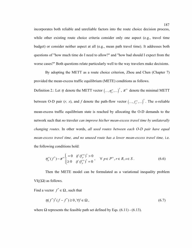
187incorporates both reliable and unreliable factors into the route choice decision process,

while other existing route choice criteria consider only one aspect (e.g., travel time

budget) or consider neither aspect at all (e.g., mean path travel time). It addresses both

questions of "how much time do I need to allow?" and "how bad should I expect from the

worse cases?" Both questions relate particularly well to the way travelers make decisions.

By adopting the METT as a route choice criterion, Zhou and Chen (Chapter 7)

provided the mean-excess traffic equilibrium (METE) conditions as follows.

Definition 2.: Let η denote the METT vector ( ), ,Trs

pη… … , rsπ denote the minimal METT

between O-D pair (r, s), and f denote the path-flow vector ( ), ,Trs

pf… … . The α-reliable

mean-excess traffic equilibrium state is reached by allocating the O-D demands to the

network such that no traveler can improve his/her mean-excess travel time by unilaterally

changing routes. In other words, all used routes between each O-D pair have equal

mean-excess travel time, and no unused route has a lower mean-excess travel time, i.e.

the following conditions hold:

*

**

0 ) 0( ) , , ,

0 ) 0

rsprs rs rs

p rsp

if (ff p P r R s S

if (f η π

⎧ = >⎪− ∀ ∈ ∈ ∈⎨≥ =⎪⎩. (6.6)

Then the METE model can be formulated as a variational inequality problem

VI(f,Ω) as follows.

Find a vector *f ∈Ω , such that

* *( ) ( ) 0Tf f fη − ≥ , f∀ ∈Ω , (6.7)

where Ω represents the feasible path set defined by Eqs. (6.11) - (6.13).

188It can be proved that the VI formulation is equivalent to the METE model, and

there exists at least one equilibrium solution (Chapter 7). In the next section, we will

derive the analytical form of the path travel time distribution from the given travel

demand distribution.

Path travel time distribution

Assume the random travel demand rsQ has mean rsq and variance rsε . Then, the

path flow rspF , and link flow aV are also random variables, which consequently induce

the random path/link travel times. Let ∆ = [ rspaδ ] denote the path-link incidence matrix,

where 1=rspaδ if path p from origin r to destination s uses link a, and 0, otherwise. Then,

we have the following relationships:

, ,rs

rs rsp

p P

Q F r R s S∈

= ∀ ∈ ∈∑ , (6.8)

,rs

rs rsa p pa

r R s S p P

V F a Aδ∈ ∈ ∈

= ∀ ∈∑∑ ∑ , (6.9)

0, , ,rs rspF p P r R s S≥ ∀ ∈ ∈ ∈ , (6.10)

where (6.8) is the travel demand conservation constraint; (6.9) is a definitional constraint

that sums up all path flows that pass through a given link a; and (6.10) is a non-negativity

constraint on the path flows.

Furthermore, let rspf and av be the mean path flow and mean link flow,

respectively. Then, we have

∑∈

∈∈∀=rsPp

rsp

rs SsRrfq ,, , (6.11)

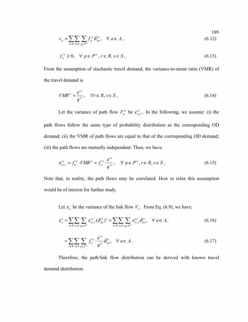
189 Aafv

Rr Ss Pp

rspa

rspa

rs

∈∀=∑∑ ∑∈ ∈ ∈

,δ , (6.12)

SsRrPpf rsrsp ∈∈∈∀≥ ,,,0 , (6.13)

From the assumption of stochastic travel demand, the variance-to-mean ratio (VMR) of

the travel demand is

rs

rsrsVMR

qε= , ,r R s S∀ ∈ ∈ , (6.14)

Let the variance of path flow rspF be ,

rsp fε . In the following, we assume: (i) the

path flows follow the same type of probability distribution as the corresponding OD

demand; (ii) the VMR of path flows are equal to that of the corresponding OD demand;

(iii) the path flows are mutually independent. Then, we have:

,

rsrs rs rs rsp f p p rsf VMR f

qεε = ⋅ = ⋅ , , ,rsp P r R s S∀ ∈ ∈ ∈ , (6.15)

Note that, in reality, the path flows may be correlated. How to relax this assumption

would be of interest for further study.

Let aε be the variance of the link flow aV . From Eq. (6.9), we have:

2, ,( ) ,

rs rs

v rs rs rs rsa p f pa p f pa

r R s S r R s Sp P p P

a Aε ε δ ε δ∈ ∈ ∈ ∈∈ ∈

= = ∀ ∈∑∑ ∑ ∑∑ ∑ , (6.16)

,rs

rsrs rs

p parsr R s S p P

f a Aqε δ

∈ ∈ ∈

= ⋅ ∀ ∈∑∑ ∑ . (6.17)

Therefore, the path/link flow distribution can be derived with known travel

demand distribution.

190The case of lognormal travel demand distribution

Though the normal distribution has been used in the literature (Chen, Subprasom,

and Ji, 2003; Shao et al., 2006) for modeling the stochastic travel demand, it may not be

appropriate to reflect the real world situations. To better model the uncertain

environment, in this study, we are particularly interested in the lognormal distribution,

which is a nonnegative, asymmetrical distribution and has been adopted in the literature

as a more realistic approximation of the stochastic travel demand to examine the

uncertainty of the four-step travel demand forecasting model (Zhao and Kockelman,

2002). The probability density function of the lognormal distribution is given as follows.

( )( )2

2ln21| ,

2

x

f x ex

µσµ σ

σ π

− −

= , 0x∀ > , (6.18)

where x is the random variable, µ and σ are the distribution parameters, and the mean

and variance are 22σµ+= em and ( )2 22 1v e eµ σ σ+= − , respectively. Based on the

assumptions above, the distribution parameters of the random path flows can be derived

as follows (Aitchison and Brown, 1957):

( )( )

,, 2

1ln ln 12

rsp frs rs

p f p rsp

ff

εµ

⎛ ⎞⎜ ⎟= − +⎜ ⎟⎝ ⎠

, , ,rsp P r R s S∀ ∈ ∈ ∈ , (6.19)

( )( )

2 ,, 2ln 1

rsp frs

p f rspf

εσ

⎛ ⎞⎜ ⎟= +⎜ ⎟⎝ ⎠

, , ,rsp P r R s S∀ ∈ ∈ ∈ . (6.20)

Consequently, the path flows also follow the lognormal distribution:

( )rsfp

rsfp

rsp LNF ,, ,~ σµ , , ,rsp P r R s S∀ ∈ ∈ ∈ . (6.21)

191According to the path-link relationship in Eq. (6.9), the distribution parameters of the

random link flows can be approximated (Fenton, 1960) as follows:

( ) 2

1ln ln 12

vv aa a

a

vvεµ

⎛ ⎞= − +⎜ ⎟

⎝ ⎠, a A∀ ∈ , (6.22)

( )2

2ln 1v

v aa

avεσ

⎛ ⎞= +⎜ ⎟

⎝ ⎠, a A∀ ∈ , (6.23)

( )va

vaa LNV σµ ,~ , a A∀ ∈ . (6.24)

Now, consider the strictly increasing link travel time function

( )a a aT Vλ= , a A∀ ∈ , (6.25)

where the mean and variance of link travel time can be represented as:

( ) ( ) ( )| ,v va a a a at E T x f x dxλ µ σ

+∞

−∞= = ∫ , a A∀ ∈ , (6.26)

( ) 2ta a aE T E Tε = −⎡ ⎤⎣ ⎦

( ) ( ) ( ) ( )( )22 2| , | ,v v v va a a a a ax f x dx x f x dxλ µ σ λ µ σ

+∞ +∞

−∞ −∞= −∫ ∫ , a A∀ ∈ (6.27)

Assume ( )a aVλ to be the standard Bureau of Public Road (BPR) function as below:

( ) 0 1 ,n

aa a a a

a

VT V t a AC

λ β⎛ ⎞⎛ ⎞⎜ ⎟= = + ∀ ∈⎜ ⎟⎜ ⎟⎝ ⎠⎝ ⎠

, (6.28)

where 0at is the link free-flow travel time, aC is the link capacity, n and β are parameters.

Using Eqs. (6.24) - (6.28), and performing some calculus manipulations, the mean and

variance of link travel time based on the BPR function can be derived as follows.

( )22

00 2

vav

a

nna

a a na

tt t eC

σµβ +

⎛ ⎞⎜ ⎟= +⎜ ⎟⎜ ⎟⎝ ⎠

, a A∀ ∈ , (6.29)

192

( ) ( )2 22 220

21( )

v v va a an n nt a

a na

t e eC

σ µ σβε +⎛ ⎞ ⎡ ⎤= − ⋅⎜ ⎟ ⎢ ⎥⎣ ⎦⎝ ⎠, a A∀ ∈ . (6.30)

Using the path-link incidence relationship, the random path travel time can be expressed

as:

rs rsp a pa

aT T δ=∑ , , ,rsp P r R s S∀ ∈ ∈ ∈ . (6.31)

To facilitate the presentation of the essential ideas, we assume the link travel times are

independent. Hence, the mean and variance of rspT can be written as:

rs rsp a pa

at t δ=∑ , , ,rsp P r R s S∀ ∈ ∈ ∈ , (6.32)

,rs t rsp t a pa

aε ε δ=∑ , , ,rsp P r R s S∀ ∈ ∈ ∈ , (6.33)

According to the Central Limit Theorem, for paths consisting of many links, the

random path travel times tend to the normal distribution regardless of what the

underlying link travel time distribution is (Lo and Tung, 2003; Shao et al., 2006):

( )( )2

,~ ,rs rs rsp p p tT N t σ , , ,rsp P r R s S∀ ∈ ∈ ∈ , (6.34)

where , ,

rs rsp t p tσ ε= , , ,rsp P r R s S∀ ∈ ∈ ∈ . (6.35)

Note that, in reality, the link travel times may not be independent due to the

network topology or the sources of variations. Therefore, the effects of the covariance of

link travel times should be considered in future research. A recent attempt in this

direction can be found in Lam, Shao, and Sumalee (2008).

Assume the confidence level is α, then the METT, according to Eq. (6.4), can be

expressed as

193

( ) ( )( )

( )( )( )

2

,2

, ,

1 1 exp1 2 2

rsp

rs rsp p trs rs rs

p p prs rsp t p t

TT d T

ξ α

µη α

α πσ σ

∞⎛ ⎞−⎜ ⎟= ⋅ −⎜ ⎟−⎝ ⎠

∫ . (6.36)

Equivalently, based on Eq. (6.5), the METT can also be expressed as follows.

( ) ( ) ( ) ( )0

11

rs rs rs rs rsp p p p pT d Tη α ξ α ξ α

α

+∞⎡ ⎤= + −⎣ ⎦− ∫ , (6.37)

where ( )rspξ α is exactly the TTB of path p under a confidence level α, which can be

expressed as a function of mean and standard deviation of path travel time:

( ) ( ) rstp

rsp

rsp t ,

1 σααξ ⋅Φ+= − . (6.38)

Following some calculus manipulations, the METT can be further expressed as:

( )( )

( )( ) ( )21

, 1,exp

22 1

rsp trs rs rs

p p p t

αση ξ α α σ

π α

−−

⎛ ⎞⎛ ⎞Φ⎜ ⎟⎜ ⎟= + − − Φ ⋅⎜ ⎟⎜ ⎟−

⎝ ⎠⎝ ⎠

. (6.39)

By substituting Eq. (6.38) into Eq. (6.39), we can see that the METT can be

further decomposed into three individual terms: the first term is the mean travel time, the

second term is the “buffer time” that the travelers allowed to ensure the travel time

reliability requirement, and the third term accounts for the expected impacts from the

excessively late trips (i.e., bad days with extremely high travel times). Thus, it is clear

that the three user equilibrium models (i.e., UE, DRUE and METE) can be distinguished

by considering different combinations of the three terms. If only the first term is

considered, it generates the UE model in which the travel time variability is disregarded

in the route choice decision process and is unable to reflect the travelers' risk preference.

In this model, travelers will be late about half of the time and early the other half of the

time if they plan their trips based on the average travel time. If the first two terms are

194considered, it generates the DRUE model that only accounts for the acceptable risk

defined by the travelers' reliability requirement at a confidence level α. In this model, if

travelers plan their trips based on TTB with a confidence level α (e.g., 90th percentile of

travel time), they will be late about two working days per month (assuming there are 20

working days per month). These late trips with unacceptable travel times experienced and

suffered by the travelers (i.e., bad days) are the ones they remember the most. Finally, if

all three terms are considered, it generates the METE model, which accounts for the

travelers' risk preference on both acceptable and unacceptable risks. In this model,

travelers consider the possibility that the unacceptable travel times in the tail are

excessively higher than the TTB, and add the mean-excess time (third term) to minimize

the risk of encountering those bad days. Among the three UE models considered in this

comparative analysis, the METE model is the most conservative one.

Numerical Results

Since the METT is nonadditive in general (i.e., the path cost is not simply the sum

of the link costs that constitute that path), the METE model can be regarded as a

nonadditive user equilibrium problem and a path-based traffic assignment algorithm is

needed (Lo and Chen, 2000; Chen, Lo, and Yang, 2001; Zhou and Chen, 2006).

Recently, Zhou and Chen (Chapter 7) developed a modified alternating direction method

for solving the METE model. The algorithm has several good features that enable it for

solving large-scale problems.

To illustrate the differences among the three user equilibrium models (i.e., UE,

DRUE and METE models), a simple network with 10 nodes, 11 links, and two OD pairs

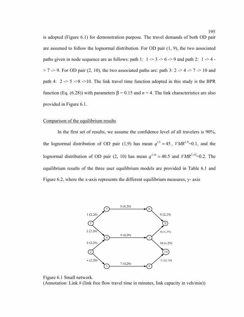
195is adopted (Figure 6.1) for demonstration purpose. The travel demands of both OD pair

are assumed to follow the lognormal distribution. For OD pair (1, 9), the two associated

paths given in node sequence are as follows: path 1: 1 -> 3 -> 6 -> 9 and path 2: 1 -> 4 -

> 7 -> 9. For OD pair (2, 10), the two associated paths are: path 3: 2 -> 4 -> 7 -> 10 and

path 4: 2 -> 5 ->8 ->10. The link travel time function adopted in this study is the BPR

function (Eq. (6.28)) with parameters β = 0.15 and n = 4. The link characteristics are also

provided in Figure 6.1.

Comparison of the equilibrium results

In the first set of results, we assume the confidence level of all travelers is 90%,

the lognormal distribution of OD pair (1,9) has mean 1,9 45q = , VMR1,9=0.1, and the

lognormal distribution of OD pair (2, 10) has mean 2,10 40.5q = and VMR2,10=0.2. The

equilibrium results of the three user equilibrium models are provided in Table 6.1 and

Figure 6.2, where the x-axis represents the different equilibrium measures, y- axis

Figure 6.1 Small network. (Annotation: Link # (link free flow travel time in minutes, link capacity in veh/min))

196represents the different models, and z-axis represents the corresponding measurement

values of the given model and measurement combination. For simplicity, only the results

of path 1 and path 2 are presented in the figure, and the mean travel time, travel time

budget and mean-excess travel time are abbreviated by MTT, TTB, and METT,

respectively.

First, from the table, we can see that the mean path flows sum up to the mean OD

travel demands and the corresponding equilibrium measures of all used paths for each

OD pair are equal and minimal. They demonstrate the validity of the results. Second, it is

clear that the three user equilibrium models give different equilibrium path-flow patterns

(albeit the differences are small in this example). The reason for the difference is based

on the different criteria used to represent travelers’ risk preference in their route choice

decisions (see Figure 6.2). For example, when the traditional UE model is adopted, at

Table 6.1 Equilibrium results of different user equilibrium models

Model Path # Path flow (veh/min) MTT (min) TTB (min) METT (min)

1 26.46 11.76 12.50 12.77 2 18.54 11.76 11.93 11.99 3 13.69 13.56 13.71 13.77

UE

4 26.81 13.56 14.88 15.37 1 25.85 11.43 12.11 12.36 2 19.15 11.91 12.11 12.18 3 14.92 13.72 13.92 13.99

DRUE

4 25.58 12.79 13.92 14.33 1 25.67 11.33 12.00 12.24 2 19.33 11.95 12.16 12.24 3 15.27 13.77 13.98 14.06

METTUE

4 25.23 12.58 13.66 14.06

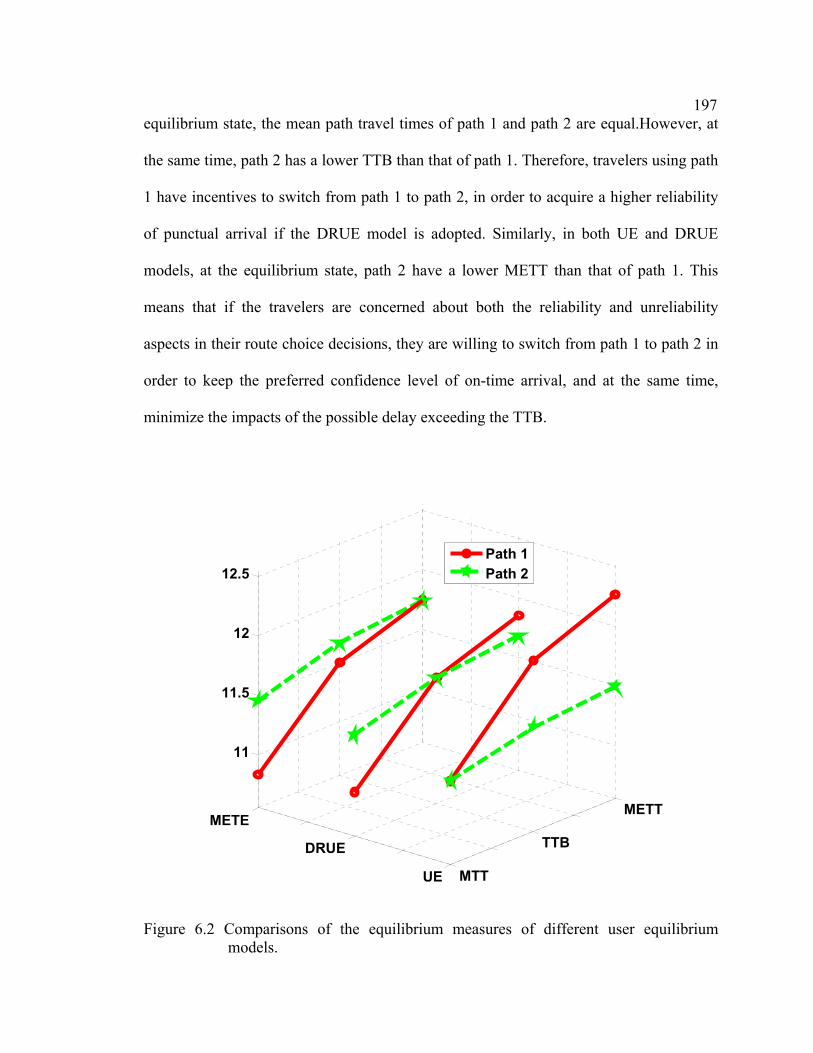
197equilibrium state, the mean path travel times of path 1 and path 2 are equal.However, at

the same time, path 2 has a lower TTB than that of path 1. Therefore, travelers using path

1 have incentives to switch from path 1 to path 2, in order to acquire a higher reliability

of punctual arrival if the DRUE model is adopted. Similarly, in both UE and DRUE

models, at the equilibrium state, path 2 have a lower METT than that of path 1. This

means that if the travelers are concerned about both the reliability and unreliability

aspects in their route choice decisions, they are willing to switch from path 1 to path 2 in

order to keep the preferred confidence level of on-time arrival, and at the same time,

minimize the impacts of the possible delay exceeding the TTB.

MTT

TTB

METT

UE

DRUE

METE

11

11.5

12

12.5

Path 1Path 2

Figure 6.2 Comparisons of the equilibrium measures of different user equilibrium models.

198Finally, the relations among different equilibrium route choice criteria are graphically

illustrated in Figure 6.3. For simplicity, we only show the equilibrium results of path 1

and path 2 under the METE model. The dashed line represents the probability density

function, while the solid line represents the cumulative distribution function. From the

figure, we can observe that for each path, the TTB is always greater than the MTT due to

the consideration of the travel time reliability requirement at a confidence level α. At the

same time, the METT is always higher than the TTB, since it takes into account of the

unreliability impacts represented by the shaded area of the tail with a probability 1-α.

9 9.5 10 10.5 11 11.5 12 12.5 13 13.5 140

0.5

1

P a t h 1 T r a v e l T i m e

P r o

b a

b i

l i t

y D

e n

s i

t y

9 9.5 10 10.5 11 11.5 12 12.5 13 13.5 140

0.1

0.2

0.3

0.4

0.5

0.6

0.7

0.8

0.9

1

P r o

b a

b i

l i t

y

M e a n T r a v e l T i m e

T r a v e l T i m e B u d g e t

C o n f i d e n c e L e v e l

M e a n E x c e s s T r a v e l T i m e

11.33 12.0012.24

11 11.2 11.4 11.6 11.8 12 12.2 12.4 12.6 12.8 130

0.5

1

1.5

2

2.5

P a t h 2 T r a v e l T i m e

P r o

b a

b i

l i t

y D

e n

s i

t y

11 11.2 11.4 11.6 11.8 12 12.2 12.4 12.6 12.8 130

0.1

0.2

0.3

0.4

0.5

0.6

0.7

0.8

0.9

1

P r o

b a

b i

l i t

y

M e a n T r a v e l T i m e

T r a v e l T i m e B u d g e t

C o n f i d e n c e L e v e l

M e a n E x c e s s T r a v e l T i m e

11.95 12.16 12.24

Figure 6.3 Comparison among different route choice criteria (path 1 and path 2).

199Analysis of the variations of demand level and confidence level

Without loss of generality, we assume all travelers’ travel time requirement given

in terms of a confidence level is 90%, the base OD demands are 1,9 30q = , 2,10 27q = ,

VMR1,9=0.1, and VMR2,10=0.2. Here, we examine the link flow variation on link 6 at the

equilibrium state of the METE model under different demand levels: ( )1,9 2,10,q q qλ= ⋅ ,

where λ = 1.0, 1.1,…, 2.0 is the multiplier that represents the demand level from 1 to 11,

respectively. Figure 6.4 graphically depicts the probability density functions of the flow

distribution on link 6 with respect to different demand levels. From the figure, we can

observe that an increase of the mean and variance of OD demands leads to an increase of

the mean (v) and variance (ε) of the link flow distribution. Therefore, Figure 6.4 indeed

illustrates that the link flow is actually random due to the stochastic travel demand.

In the following, the effect of demand variations on the equilibrium results for

each model is explored. Since the results of both OD pairs are similar, only the results of

OD pair (1, 9) are shown in Figure 6.5. It is clear that the MTT, TTB, and METT

increase as the demand level increases and METT ≥ TTB ≥ MTT. Furthermore, the

differences among them get larger when the demand level increases. Due to the

congestion effect, all of the measures have a higher rate of increase at higher demand

levels than that at lower demand levels. This implies that the consideration of both

reliability and unreliability aspects of travel time variability may has a more significant

effect on travelers' route choice decision under heavier congestion levels, and the price

for maintaining the travel time reliability requirement and avoiding the unreliability

impacts are also higher. For example, knowing that the congestion is severe, travelers

200

0 10 20 30 40 50 600

0.05

0.1

0.15

0.2

0.25

0.3

0.35

0.4

L i n k F l o w

P r o

b a

b i

l i t

y D

e n

s i

t y

D e m a n d L e v e l 1(v

a = 9.78, ε

a = 1.30)

D e m a n d L e v e l 11(v

a = 52.86, ε

a = 7.70)

F r o m D e m a n d L e v e l 1 to 11

Figure 6.4 Link flow distributions of link 6 under different demand levels. have to depart earlier to ensure more frequent on-time arrival and to minimize the

associated risk of encountering excessively high delay.

Now, we fix the OD demand to be 1,9 54q = , 2,10 48.6q = , VMR1,9=0.1, and

VMR2,10=0.2, and examine the effect of different confidence levels. Based on the

discussions in the previous sections, it is reasonable to assume that all travelers are risk-

averse under an uncertain environment. Therefore, we only consider the situation that the

travelers' confidence level 50%α ≥ . Here, only the results of OD pair (1, 9) are

examined in Figure 6.6. From the figure, the following observations can be drawn:

The equilibrium MTT remains unchanged for all confidence levels. This is because

the UE model does not account for travel time variability in the route choice decision

process.

The equilibrium TTB and METT are both increasing as the confidence level

increases. This is to be expected since travelers need to budget extra time in order to

201

1 2 3 4 5 6 7 8 9 10 1110

11

12

13

14

15

16

17

18

D e m a n d L e v e l

T r a

v e

l T

i m

e I

n d

e x

( m

i n

)

M e a n T r a v e l T i m eT r a v e l T i m e B u d g e tM e a n E x c e s s T r a v e l T i m e

Figure 6.5 Equilibrium results under different demand levels.

satisfy a higher travel time reliability requirement given by the increasing α value

The METT is always higher than the TTB. As the confidence level approaches 1.0,

the two measures get closer to each other. This phenomenon is consistent with the

TTB and METT definitions and can be derived from the relationship given in Eq.

(6.39).

At the confidence level 0.5, the MTT and TTB are identical, which implies the DRUE

model is equivalent with UE model. However, the METT given by the METE model

is still higher than the MTT since it accounts for the risk beyond the MTT.

Finally, we examine the effect of various combinations of demand level and

confidence level. As defined in the previous experiments, the demand levels are from 1 to

11, and the confidence levels are from 0.5 to 0.9. For demonstration purpose, we only

show the surface of the equilibrium METT of OD pair (1,9) in Figure 6.7. When the

demand level is low, the METTs for all confidence levels are similar. In this low demand

202

0.5 0.6 0.7 0.8 0.9 1

13.5

14

14.5

15

C o n f i d e n c e L e v e l (α)

T r a

v e

l T

i m

e I

n d

e x

( m

i n

)

M e a n T r a v e l T i m eT r a v e l T i m e B u d g e tM e a n E x c e s s T r a v e l T i m e

Figure 6.6 Equilibrium results under different confidence levels. scenario, since travel time variability is low, travelers only need to add a small amount of

extra time (buffer time + excess travel time) to improve travel time reliability and to

minimize the risk of encountering unacceptable travel time beyond TTB. The dominate

factor is the mean travel time. When the demand level is high, the METT increases in a

nonlinear fashion as the confidence level increases. This means travelers need to set aside

a larger amount of extra time to ensure both reliability and unreliability aspects of the

larger travel time variability induced by the higher demand levels. For example, the

METT value of the demand-confidence level combination (11, 0.9) is about 27% higher

than the combination (8, 0.8). Overall, Figure 6.7 provides a complete picture of the trend

of the equilibrium METT results with respect to various combinations of the demand

level and confidence level.

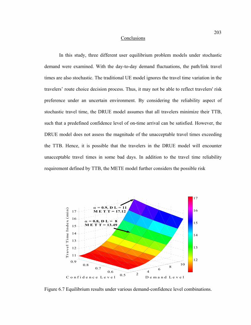
203Conclusions

In this study, three different user equilibrium problem models under stochastic

demand were examined. With the day-to-day demand fluctuations, the path/link travel

times are also stochastic. The traditional UE model ignores the travel time variation in the

travelers’ route choice decision process. Thus, it may not be able to reflect travelers' risk

preference under an uncertain environment. By considering the reliability aspect of

stochastic travel time, the DRUE model assumes that all travelers minimize their TTB,

such that a predefined confidence level of on-time arrival can be satisfied. However, the

DRUE model does not assess the magnitude of the unacceptable travel times exceeding

the TTB. Hence, it is possible that the travelers in the DRUE model will encounter

unacceptable travel times in some bad days. In addition to the travel time reliability

requirement defined by TTB, the METE model further considers the possible risk

24

68

10

0.50.6

0.70.8

0.9

11

12

13

14

15

16

17

D e m a n d L e v e lC o n f i d e n c e L e v e l

T r

a v

e l

T i m

e I

n d

e x

( m

i n

)

12

13

14

15

16

17

α = 0.9, D L = 11M E T T = 17.12

α = 0.8, D L = 8M E T T = 13.49

Figure 6.7 Equilibrium results under various demand-confidence level combinations.

204associated with the travel times beyond the TTB. The analytical form of the METT is

derived, which reveals the relationships among the different route choice criteria adopted

in the three user equilibrium models for the comparative analysis conducted in this study.

The limited numerical results showed that the three models are indeed different and

highlighted the essential ideas of the METE model, which is to consider both reliability

and unreliability aspects of handling travel time variability in the route choice decision

process.

Due to the complex situations in the real world, no UE model is sufficient in

capturing all aspects of the travelers’ risk-taking behavior in the route choice decision

process, and whether the UE, DRUE or METE model is the most realistic is an open

question. It is worthwhile to explore this issue through empirical studies given the

potential differences identified in this comparative analysis. Further work includes

extending the METE model to account for perception error to reflect that travelers may

not have perfect knowledge of the travel time distributions. Finally, developing efficient

path-based algorithms for solving the METE model in large-scale networks is also

important in implementing these advanced route models for practical applications.

References

Aitchison, J., and J. A. C. Brown. 1957. The lognormal distribution with special

reference to its uses in econometrics, Cambridge University Press, Cambridge, U.K. 194 p.

Al-Deek H., and E. B. Emam. 2006. New methodology for estimating reliability in

transportation networks with degraded link capacities. Journal of Intelligent Transportation Systems 10(3): 117-129.

205Artzner, P., F. Delbaen, J. M. Eber, and D. Heath. 1999. Coherent measures of risk.

Mathematical Finance 9: 203-228. Bell, M. G. H.， and C. Cassir. 2002. Risk-averse user equilibrium traffic assignment:

An application of game theory. Transportation Research Part B 36: 671-681. Brownstone, D., A. Ghosh, T. F. Golob, C. Kazimi, and D. V. Amelsfort. 2003. Drivers’

willingness-to-pay to reduce travel time: Evidence from the San Diego I-15 congestion pricing project. Transportation Research Part A 37(4): 373-387.

Cambridge Systematics, Inc., Texas Transportation Institute, University of Washington,

Dowling Associates. 2003. Providing a highway system with reliable travel times. NCHRP Report No. 20-58[3], Transportation Research Board, National Research Council, U.S.A.

Chen, A., and Z. Ji. 2005. Path finding under uncertainty. Journal of Advanced

Transportation 39(1): 19-37. Chen, A., H. K. Lo, and H. Yang. 2001 A self-adaptive projection and contraction

algorithm for the traffic assignment problem with path-specific costs. European Journal of Operational Research 135: 27-41.

Chen, A., K. Subprasom, and Z. Ji. 2003. Mean-variance model for the build-operate-

transfer model under demand uncertainty. Transportation Research Record 1857: 93-101.

Chen, A., H. Yang, H. K. Lo, and W. H. Tang. 2002. Capacity reliability of a road

network: An assessment methodology and numerical results. Transportation Research Part B 36:225-252.

Fenton, L. F. 1960. The sum of log-normal probability distributions in scatter

transmission systems. IEEE Transactions on Communications Systems CS-8: 57-67. FHWA. 2006. Travel time reliability: Making it there on time, all the time. Report No.

70, Federal Highway Administration. Heydecker, B. G., W. H. K. Lam., and N. Zhang. 2007. Use of travel demand satisfaction

to assess road network reliability. Transportmetrica 3(2): 139-171. Lam, W.H.K., H. Shao, and A. Sumalee. 2008. Modeling impacts of adverse weather

conditions on a road network with uncertainties in demand and supply. Submitted to Transportation Research Part B.

206Liu, H., W. Recker, and A. Chen. 2004. Uncovering the contribution of travel time

reliability to dynamic route choice using real-time loop data. Transportation Research Part A 38: 435-453.

Lo, H. K., and A. Chen. 2000. Traffic equilibrium problem with route-specific costs:

Formulation and algorithms. Transportation Research Part B 34: 493-513. Lo, H. K., X. W. Luo, and B. W. Y. Siu. 2006. Degradable transport network: Travel

time budget of travelers with heterogeneous risk aversion. Transportation Research Part B 40: 792-806.

Lo, H. K., and Y. K. Tung. 2003. Network with degradable links: Capacity analysis and

design. Transportation Research Part B 37: 345-363. Mirchandani, P., and H. Soroush. 1987. Generalized traffic equilibrium with probabilistic

travel times and perceptions. Transportation Science 21: 133-152. Noland, R. B. 1999. Information in a two-route network with recurrent and non-recurrent

congestion, p. 95-114. In R. Emmerink and P. Nijkamp (Ed.). Behavioural and Network Impacts of Driver Information Systems, Ashgate, Aldershot, UK.

Rockafellar, R. T., and S. Uryasev. 2002. Conditional value-at-risk for general loss

distributions. Journal of Banking and Finance 26(7): 1443-1471. Shao, H., W. H. K. Lam, Q. Meng, and M. L. Tam. 2006. Demand driven travel time

reliability-based traffic assignment problem. Transportation Research Record 1985: 220-230.

Watling, D. 2006. User equilibrium traffic network assignment with stochastic travel

times and late arrival penalty. European Journal of Operational Research 175: 1539-1556.

Yamai, Y., and Y. Yoshiba. 2001. On the validity of value-at-risk: Comparative analysis

with expected shortfall. Bank of Japan. IMES Discussion Paper, 2001-E-4. Zhao, Y., and K. Kockelman. M. 2002. The propagation of uncertainty through travel

demand models. Annals of Regional Science 36(1): 145-163. Zhou, Z., and A. Chen. 2006. A self-adaptive gradient projection algorithm for solving

the nonadditive traffic equilibrium problem. Presented at the 85th annual meeting of the Transportation Research Board, Washington, D.C., USA.

207CHAPTER 7

A STOCHASTIC α-RELIABLE MEAN-EXCESS TRAFFIC EQUILIBRIUM MODEL

WITH PROBABILISTIC TRAVEL TIMES AND PERCEPTION ERRORS1

Abstract

This paper proposes a novel stochastic mean-excess traffic equilibrium model that

considers both reliability and unreliability aspects of travel time variability and

perception errors within the travelers’ route choice decision processes. In the model, each

traveler not only considers a travel time budget for ensuring on-time arrival at a

confidence level α, but also accounts for the impact of encountering worst travel times in

the (1-α) quantile of the distribution tail. Furthermore, due to the imperfect knowledge of

the travel time variability, the travelers’ route choice decisions are based on the perceived

travel time distribution rather than the actual travel time distribution. In order to compute

the perceived mean-excess travel time, an approximation method based on moment

analysis is developed. The proposed model is formulated as a variational inequality (VI)

problem, and solved by a route-based algorithm based on the modified alternating

direction method. Numerical examples are also provided to illustrate the proposed model

and solution procedure.

Introduction

Traffic equilibrium problem is one of the most critical and fundamental problems

in transportation. Given the travel demand between origin-destination (O-D) pairs (i.e.,

1 Co-authored by Zhong Zhou and Anthony Chen

208travelers), and travel cost function for each link of the transportation network, the traffic

equilibrium problem determines the equilibrium traffic flow pattern and various

performance measures of the network. Route choice model is inherently embedded in the

traffic equilibrium problem to model individual route choice decisions between various

O-D pairs, while congestion is explicitly considered through the travel cost functions.

Recently, travel time variability has been emerged as an important topic due to its

significant impacts on travelers’ route choice behavior as observed by many empirical

studies (Abdel-Aty, Kitamura, and Jovanis, 1995; Small et al., 1999; Brownstone et al.,

2003; Liu, Recker, and Chen, 2004; de Palma and Picard, 2005). These studies revealed

that travelers indeed consider travel time variability as a risk in their route choice

decisions since they do not know exactly when they will arrive at the destination. Thus,

they are interested in not only travel time saving but also risk reduction when making

their route choice. However, the traditional user equilibrium (UE) neglects travel time

variability in the route choice decision process. It adopts the expected travel time as the

sole criterion for making route choices. Thus, it implicitly assumes all travelers to be risk-

neutral. Moreover, it is well recognized that travelers may not have perfect knowledge

about the network condition. Therefore, it is reasonable to incorporate the travelers’

perception error into the route choice decision process. However, similar to the UE

model, the traditional stochastic user equilibrium (SUE) model also neglects the effect of

travel time variability in the route choice decision process. It adopts the expected

perceived travel time as the sole criterion for making route choices; and hence, it also

implicitly assumes all travelers are risk-neutral.

Typically, travel time variability can be represented by two different aspects:

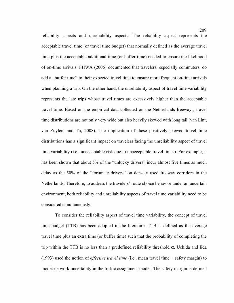
209reliability aspects and unreliability aspects. The reliability aspect represents the

acceptable travel time (or travel time budget) that normally defined as the average travel

time plus the acceptable additional time (or buffer time) needed to ensure the likelihood

of on-time arrivals. FHWA (2006) documented that travelers, especially commuters, do

add a “buffer time” to their expected travel time to ensure more frequent on-time arrivals

when planning a trip. On the other hand, the unreliability aspect of travel time variability

represents the late trips whose travel times are excessively higher than the acceptable

travel time. Based on the empirical data collected on the Netherlands freeways, travel

time distributions are not only very wide but also heavily skewed with long tail (van Lint,

van Zuylen, and Tu, 2008). The implication of these positively skewed travel time

distributions has a significant impact on travelers facing the unreliability aspect of travel

time variability (i.e., unacceptable risk due to unacceptable travel times). For example, it

has been shown that about 5% of the “unlucky drivers” incur almost five times as much

delay as the 50% of the “fortunate drivers” on densely used freeway corridors in the

Netherlands. Therefore, to address the travelers’ route choice behavior under an uncertain

environment, both reliability and unreliability aspects of travel time variability need to be

considered simultaneously.

To consider the reliability aspect of travel time variability, the concept of travel

time budget (TTB) has been adopted in the literature. TTB is defined as the average

travel time plus an extra time (or buffer time) such that the probability of completing the

trip within the TTB is no less than a predefined reliability threshold α. Uchida and Iida

(1993) used the notion of effective travel time (i.e., mean travel time + safety margin) to

model network uncertainty in the traffic assignment model. The safety margin is defined

210as a function of travel time variability, which serves as a measure of risk averseness in

their risk-based traffic assignment models. Lo, Luo, and Siu (2006) proposed a

probabilistic user equilibrium (PUE) model to account for the effects of within budget

time reliability (WBTR) due to degradable links with predefined link capacity

distributions. By assuming travel time variability is induce by the travel demand

fluctuation instead of capacity degradation, Shao et al. (2006) proposed a demand driven

travel time reliability-based user equilibrium (DRUE) model. Later, Shao et al. (2008)

further extended this approach to model the rain effects on road network with random

demand, where the link free-flow travel time and link capacity are treated as a function of

the rain intensity. The framework of the above reliability-based traffic equilibrium

models can be depicted in Figure 7.1.

Figure 7.1 Framework of the reliability-based traffic equilibrium models.

211On the other hand, to account for the unreliability aspect of travel time reliability

(i.e., unacceptable travel times), a general adopted concept to consider the unreliability

effect is schedule delay (SD). It is defined as the difference between the chosen time of

arrival and the official work start time (Small, 1982), used in conjunction with a disutility

function to model the travel choice decision (Noland et al., 1998; Noland, 1999). Watling

(2006) proposed a late arrival penalized user equilibrium (LAPUE) model by

incorporating a schedule delay term to the disutility function to penalize late arrival for a

fixed departure time. Siu and Lo (2007) showed that there is a relationship between the

risk aversion coefficient of the TTB model and the SD cost. These models can be

represented by Figure 7.2

However, note that both reliability-based and unreliability-based traffic

equilibrium models above only consider one aspect of travel time variability (i.e., either

Unreliability-based Route Choice Flow Dependent Network Congestion

Traffic Flow

Traveler

Network

Scheduled Delay (SD)Actual Travel Time

Distribution

No Perception Error

Figure 7.2 Framework of the unreliability-based traffic equilibrium models.

212the reliability aspect using the concept of TTB or the unreliability aspect using the

concept of SD). To adequately describe travelers’ route choice decision process under

travel time variability, both reliability and unreliability aspects should be explicitly

considered. Recently, Zhou and Chen (Chapter 5) proposed a α-reliable mean-excess

traffic equilibrium (METE) model, where each traveler attempts to minimize his/her

mean-excess travel time (METT), which is defined as the conditional expectation of the

travel time exceeding the TTB. As a route choice criterion, METT can be regarded as a

combination of the buffer time measure that ensures the reliability of on-time arrival, and

the tardy time measure that represents the unreliability impacts of excessively late trips

(Cambridge Systematics, et al., 2003). It incorporates both reliability and unreliability

aspects of travel time variability to simultaneously address both questions of "how much

time do I need to allow?" and "how bad should I expect from the worse cases?"

Therefore, travelers' route choice behavior can be considered in a more accurate and

complete manner in a network equilibrium framework to reflect their risk preferences

under an uncertain environment. This model can be shown as Figure 7.3.

To account for both reliability issues and travelers’ perception error, Siu and Lo

(2006) extended the PUE model to consider two types of uncertainty in travelers’ daily

commutes, i.e. uncertainty in the actual travel time due to random link degradations and

perception error variations in the TTB due to imperfect information. Shao, Lam, and Tam

(2006) also extended the DRUE model to incorporate the randomness of link travel time

from the daily demand variation and travelers’ perception error on the TTB. Similar to

the traditional logit-based SUE models (Dial, 1971; Fisk, 1980), they assume the

commonly adopted Gumbel variate as the random error term. This random error term is

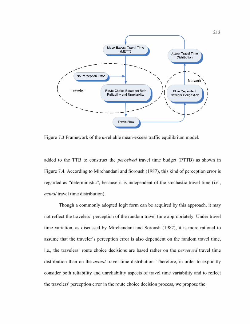
213

Figure 7.3 Framework of the α-reliable mean-excess traffic equilibrium model.

added to the TTB to construct the perceived travel time budget (PTTB) as shown in

Figure 7.4. According to Mirchandani and Soroush (1987), this kind of perception error is

regarded as “deterministic”, because it is independent of the stochastic travel time (i.e.,

actual travel time distribution).

Though a commonly adopted logit form can be acquired by this approach, it may

not reflect the travelers’ perception of the random travel time appropriately. Under travel

time variation, as discussed by Mirchandani and Soroush (1987), it is more rational to

assume that the traveler’s perception error is also dependent on the random travel time,

i.e., the travelers’ route choice decisions are based rather on the perceived travel time

distribution than on the actual travel time distribution. Therefore, in order to explicitly

consider both reliability and unreliability aspects of travel time variability and to reflect

the travelers' perception error in the route choice decision process, we propose the

214

Figure 7.4 Framework of reliability-based traffic equilibrium models with deterministic perception error.

stochastic α-reliable mean-excess traffic equilibrium model, or stochastic mean-excess

traffic equilibrium (SMETE) model for short. The new model extends the METE model

by further incorporating the travelers’ perception error. In this model, travelers are

assumed to make their route choice decision based on the perceived mean-excess travel

time (PMETT) of each alternative route, which is determined by the perceived travel time

distribution considering both distributions of the random route travel time and the

perception error. In order to compute the PMETT of each route in the stochastic network,

an approximation method based on moment analysis (i.e., conditional moment generation

function used to derive the perceived link travel time, Cornish-Fisher Asymptotic

Expansion to estimate the PTTB, and Acerbi and Tasche Approximation to estimate the

PMETT based on the PTTB) is developed in this paper. The framework of this novel

model is illustrated in Figure 7.5. This is the first attempt to integrate the traveler's

215perception error, travel time reliability and unreliability into a unified network

equilibrium framework. It provides a more complete manner for considering travelers'

route choice decisions to reflect their risk preferences under an uncertain environment

and the potential applicability for solving practical problems.

The remainder of the paper is organized as follows. In Section 2, the concept of

PMETT is introduced and the stochastic mean-excess traffic equilibrium model is

proposed. The model is formulated as a general variational inequality (VI) problem.

Qualitative properties of the model and formulation are also provided. In Section 3, a

route-based algorithm based on the modified alternating direction method is provided to

determine the equilibrium flow pattern. In Section 4, illustrative examples are presented

to demonstrate the characteristics of the proposed model and its comparison to other

related user equilibrium models. Finally, conclusions and recommendations for future

research are given in Section 5.

Model and Formulation

Definition and assumptions

Consider a strongly connected network [N, A], where N and A denote the sets of

nodes and links, respectively. Let R and S denote a subset of N for which travel demand

rsq is generated from origin r R∈ to destination s S∈ and let rspf denote the flow on

route rsp P∈ , where rsP is a set of routes from origin r to destination s. Let aT represent

the random travel time on link a A∈ , which is parameterized by link flow av .

Consequently, the travel time on route rsPp ∈ between origin r to destination s is also a

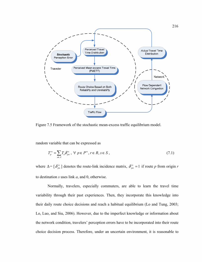
216

Figure 7.5 Framework of the stochastic mean-excess traffic equilibrium model. random variable that can be expressed as

rs rsp a pa

a AT T δ

∈

=∑ , , ,rsp P r R s S∀ ∈ ∈ ∈ , (7.1)

where ∆ = [ rspaδ ] denotes the route-link incidence matrix, 1=rs

paδ if route p from origin r

to destination s uses link a, and 0, otherwise.

Normally, travelers, especially commuters, are able to learn the travel time

variability through their past experiences. Then, they incorporate this knowledge into

their daily route choice decisions and reach a habitual equilibrium (Lo and Tung, 2003;

Lo, Luo, and Siu, 2006). However, due to the imperfect knowledge or information about

the network condition, travelers’ perception errors have to be incorporated into their route

choice decision process. Therefore, under an uncertain environment, it is reasonable to

217assume that travelers make their route choice decisions based on the perceived travel time

distribution rather than the actual one. This can be illustrated in Figure 7.6, which shows

a hypothetical travel time distribution and the corresponding travel time distribution

perceived by travelers. Due to the differences between the actual travel time distribution

(depicted in dot line) and the perceived travel time distribution (depicted in solid line),

the travelers’ route choice decisions could be quite distinct.

In the following, we give specific assumptions on the perception error used to

develop the stochastic mean-excess traffic equilibrium model with probabilistic travel

times and perception errors:

Assumption 1. The perception error distribution of an individual traveler for a segment of

road with unit travel time is ( )2,N µ σ , where ( )2,N µ σ denotes a normal distribution

with mean µ and variance 2σ .

Travel Time Distribution

Perceived Travel Time Distribution

Figure 7.6 Actual travel time distribution and perceived travel time distribution.

218Assumption 2. Traveler’s perception errors are independent for nonoverlapping route

segments.

Assumption 3. Travelers’ perception errors are mutually independent over the population

of travelers.

Note that, in our assumptions above, the parameters µ and 2σ of the normal

distribution ( )2,N µ σ are predefined and deterministic. This is distinct from the

assumptions proposed by Mirchandani and Soroush (1987), where the parameters µ and

2σ are also stochastic variables with given distributions. Though the stochastic

parameters µ and 2σ have the advantage to represent characteristics (e.g., income) that

vary from one individual to another, it requires the models to be appropriately

aggregated. Such aggregation adds complexity to the model and may significantly

increase the computational overhead. For example, the Monte Carlo simulation, which is

known as a time-consuming procedure, has been adopted by Mirchandani and Soroush

(1987) to take account for the randomly distributed parameters ( µ and 2σ ) in the

estimation of perceived route disutility. Therefore, in order to facilitate the representation

of the essential ideas, in this study, we assume all travelers come from a single group and

have similar attributes. This kind of aggregation simplifications has been widely adopted

in various travel demand models, such as mode choice, destination choice, and route

choice models (see, e.g., Sheffi, 1985; Oppenheim, 1995). Therefore, based on the

assumptions in this study, computational intensive simulation can be avoided, and

efficient moment-based analysis of the perceived travel time distribution and new route

choice criteria can be derived.

219According to Assumptions 1 to 3, the traveler’s perception error on route p and

link a can be denoted as | rsp

rsp T

ε and |aa Tε , which are conditional on the stochastic

route/link travel time rspT and aT , respectively. Then, the perceived travel time rs

pT ( aT )

can be rationally assumed as the actual travel time rspT ( aT ) plus the perception error

| rsp

rsp T

ε ( |aa Tε ), and the following equation is satisfied

| , , ,rsp

rs rs rs rsp p p T

T T p P r R s Sε= + ∀ ∈ ∈ ∈ (7.2)

( )|a

rsa a T pa

a AT ε δ

∈

= +∑ (7.3)

rsa pa

a AT δ

∈=∑ (7.4)

From the above equations, it is easy to see that travelers’ perceived travel time is

in fact dependent on the actual travel time. In other words, the perceived distribution of

the travel time is conditional on the actual distribution of the stochastic travel time. This

distinguishes our approach from the logit-based SUE approach adopted in the recent

developed reliability-based traffic equilibrium models (Siu and Lo, 2006; Shao, Lam, and

Tam, 2006), where the perception error term is independent of the stochastic travel time,

because it was assumed to be an independently and identically distributed (IID) Gumbel

variate.

In the next section, we will see how the travelers hedge against travel time

variability and make their route choice decisions to reach a long term habitual

equilibrium state while recognizing the perception of actual travel time distribution is

subject to error.

220Route choice criterion under an uncertain environment

According to Mirchandani and Soroush (1987), travelers making route choice

decisions under an uncertain environment can be categorized into three groups according

to their attitudes toward risk (i.e., risk-prone, risk-neutral and risk-averse). In the

traditional UE and SUE models, travelers are assumed to be risk-neutral since they make

their route choice decisions solely based on the (perceived) expected travel time.

However, recent empirical studies (Brownstone et al., 2003; Liu, Recker, and Chen,

2004; de Palma and Picard, 2005) revealed that most travelers are actually risk-averse.

They are willing to pay a premium to avoid congestion and minimize the associated risk.

By considering the travel time reliability requirement, travelers are searching for a

route such that the corresponding TTB allows for on-time arrival with a predefined

confidence level α (Shao et al., 2006). Meanwhile, they are also considering the impacts

of excessively late arrival (i.e., the unreliable aspect of travel time variability) and its

explicit link to the travelers' preferred arrival time in the route choice decision process

(Watling, 2006). Therefore, it is reasonable for travelers to choose a route such that the

travel time reliability requirement (i.e., acceptable travel time defined by TTB) is ensured

most of the time and the expected unreliability impact (i.e., unacceptable travel time

exceeding TTB) is minimized. This trade-off between the reliable and unreliable aspects

in travelers' route choice decision process was represented by the mean-excess route

travel time defined by Zhou and Chen (Chapter 5) as follows:

Definition 1. (Mean-Excess Travel Time) The mean-excess travel time ( )rspη α for a route

rsPp ∈ between origin r to destination s with a predefined confidence level α is equal to

221the conditional expectation of the travel time exceeding the corresponding route travel

time budget ( )rspξ α , i.e.,

( ) ( )[ | ]rs rs rs rsp p p pE T Tη α ξ α= ≥ , , ,rsp P r R s S∀ ∈ ∈ ∈ , (7.5)

where E[⋅] is the expectation operator, and ( )rspξ α is the travel time budget on route p

from origin r to destination s defined by the travel time reliability chance constraint at a

confidence level α in Eq. (7.6):

( ) ( ) min | Prrs rsp pTξ α ξ ξ α= ≤ ≥ , (7.6)

( ) ( )rs rsp pE T γ α= + , , ,rsp P r R s S∀ ∈ ∈ ∈ , (7.7)

where ( )rspγ α is the extra time added to the mean travel time as a ‘buffer time’ to ensure

more frequent on-time arrivals at the destination under the travel time reliability

requirement at a confidence level α. Note that Eq. (7.7) is exactly the definition of the

TTB defined by Chen and Ji (2005), Lo, Luo, and Siu (2006), and Shao et al. (2006).

To incorporate the travelers’ perception error, similar to definition 1 above, we

can define the perceived mean-excess travel time ( )rspη α as follows:

Definition 2. (Perceived Mean-Excess Travel Time) The perceived mean-excess travel

time ( )rspη α for a route rsPp ∈ between origin r to destination s with a predefined

confidence level α is equal to the conditional expectation of the perceived travel time

exceeding the corresponding perceived route travel time budget ( )rspξ α , i.e.,

( ) ( )[ | ]rs rs rs rsp p p pE T Tη α ξ α= ≥ , , ,rsp P r R s S∀ ∈ ∈ ∈ , (7.8)

222where rs

pT is the perceived travel time on route p between origin r to destination s , and

and ( )rspξ α is the perceived travel time budget (PTTB), defined by

( ) ( ) min | Prrs rsp pTξ α ξ ξ α= ≤ ≥ (7.9)

( ) ( )rs rsp pE T γ α= + , , ,rsp P r R s S∀ ∈ ∈ ∈ , (7.10)

where ( )rspγ α is the perceived “buffer time” added to the perceived mean travel time to

ensure the predefined travel time reliability at a confidence level α.

According to the definition above, it is easy to see that if the perceived route

travel time distribution ( )rspf T is known, the perceived mean-excess travel time

( )rspη α can be represented as:

( ) ( )( )

( )11 rs rs

p p

rs rs rs rsp p p p

T

T f T d Tξ α

η αα ≥

=− ∫ . (7.11)

Moreover, Eq. (7.11) can be restated as:

( ) ( ) ( ) ( )|rs rs rs rs rs rsp p p p p pE T Tη α ξ α ξ α ξ α⎡ ⎤= + − ≥⎣ ⎦ . (7.12)

Therefore, the PMETT can be decomposed into two individual components. The

first component is exactly the PTTB of route p, which reflects the perceived reliability

aspect of acceptable risk allowed by the travelers at a confidence level α. The second

component can be regarded as a kind of “perceived expected delay” for choosing the

current route to reflect the perceived unreliable aspect of unacceptable risk (i.e.,

perceived trip time exceeding the acceptable travel time defined by PTTB). Clearly, as a

new route choice decision criterion, the PMETT incorporates reliable and unreliable

aspects of the travel time variability and perception error into the route choice decision

223process. It addresses both questions of "how much time do I need to allow?" and "how

bad should I expect from the worse cases?" according to the travelers’ perception of the

actual travel time distribution (i.e., knowledge of network conditions). Both questions

relate particularly well to the way travelers make decisions.

Perceived mean-excess route travel time

In the literature, several possible travel time distributions have been suggested to

describe the travel time variation under an uncertain environment. For example,

exponential and uniform travel time distributions were adopted in Noland and Small

(1995) for studying the morning commuting problem. A family of distributions known as

the “Johnson curves” was studied by Clark and Watling (2005) to model the total

network travel time under random demand. Gamma type distributions were tested by Fan

and Nie (2006) in the stochastic optimal routing problem. Multivariate normal

distribution was considered by Lo, Luo, and Siu (2006), Siu and Lo (2006), Shao et al.

(2006), and Shao, Lam, and Tam (2006), where the link travel time variation was

introduced by link capacity degradation or demand fluctuation. A mixture of normal

distribution was suggested in Watling (2006). In this study, the SMETE model and its VI

formulation are proposed in a generic sense, that is, flexible travel time probability

density functions are allowed. They provide a simple, convenient representation of risk,

which fits quite well to the way that travelers' assess their trip times and risks, and make

their route choice decisions accordingly.

To determine the PMETT of a route, the cumulative density function (CDF) is

required. However, in real application, this information is generally unknown. Under

224certain special assumption (such as the normal distribution), the route travel time

distribution can be derived from the given distribution of the link travel time

distributions. However, in reality, even the link travel time distributions are given, it may

still be difficult to analytically derive the route travel time distribution. This becomes

much more complicated when the travelers’ perception error is incorporated and the

perceived travel time distribution needs to be derived. To overcome this difficulty, an

approximation scheme is adopted in this study, such that we are able to estimate the

PMETT without the need to know the explicit form of the perceived route CDF.

From assumption 1, the perception error for an unit travel time, denoted by 1|tε = ,

is a sample from ( )2,N µ σ . Moreover, according to assumption 2, the travel time on link

a is the sum of independent unit travel times. Therefore, the conditional perception error

for link a with deterministic travel time 0at is normally distributed as:

( )00 2 0| ,

a aa a aT t

N t tε µ σ=∼ (7.13)

with conditional moment generating function (MGF)

( )0

2 0 20

| exp2a T ta a

aa

t sM s t sεσµ

=

⎛ ⎞= +⎜ ⎟

⎝ ⎠

2

0exp2a

sst σµ⎡ ⎤⎛ ⎞

= +⎢ ⎥⎜ ⎟⎝ ⎠⎣ ⎦

, (7.14)

where s is a real number.

Then, the MGF of the perceived travel time aT of link a for an individual traveler is

( ) ( )expa aTM s E sT⎡ ⎤= ⎣ ⎦

225 ( ) exp a aE s T ε⎡ ⎤= +⎣ ⎦

( ) ( ) |exp exp |a a T aaT a a TE sT E sε ε⎡ ⎤= ⎣ ⎦

( ) ( ) |expa a TaT aE sT M sε= , (7.15)

where [ ]xE ⋅ denotes the expectation with respect to random variable x. Substituting

(7.14) to (7.15), we have

( )2

exp 12aa T aT

sM s E sT σµ⎧ ⎫⎡ ⎤⎛ ⎞⎪ ⎪= + +⎨ ⎬⎢ ⎥⎜ ⎟

⎝ ⎠⎪ ⎪⎣ ⎦⎩ ⎭ (7.16)

2

12aT

sM s σµ⎡ ⎤⎛ ⎞

= + +⎢ ⎥⎜ ⎟⎝ ⎠⎣ ⎦

. (7.17)

Thus, by taking the first derivative of the MGF above and evaluating at s = 0, we can

easily acquire the first moment (i.e., mean) of the perceived travel time distribution

( ) [ ]1a aE T E Tµ⎡ ⎤ = +⎣ ⎦ , (7.18)

where ( )aE T is the mean of the random travel time aT . Similarly, the second to fourth

moments of the perceived travel time distribution can be derived from the corresponding

order of derivative evaluated at s = 0

( ) [ ]22 2 2( ) 1 ( )a a aE T E T E Tµ σ⎡ ⎤ ⎡ ⎤= + +⎣ ⎦⎣ ⎦ (7.19)

( ) ( )33 3 2 2( ) 1 ( ) 3 1 ( )a a aE T E T E Tµ µ σ⎡ ⎤ ⎡ ⎤ ⎡ ⎤= + + +⎣ ⎦ ⎣ ⎦⎣ ⎦ (7.20)

( ) ( )4 24 4 2 3 4 2( ) 1 ( ) 6 1 ( ) 3 ( )a a a aE T E T E T E Tµ µ σ σ⎡ ⎤ ⎡ ⎤ ⎡ ⎤ ⎡ ⎤= + + + +⎣ ⎦ ⎣ ⎦ ⎣ ⎦⎣ ⎦ . (7.21)

Consequently, the second to fourth central moments of the perceived travel time

distribution can be represented as follows.

226

( ) ( ) ( )222 2( ) ( )a a a a aE T E T E T E Tλ ⎡ ⎤ ⎡ ⎤ ⎡ ⎤= − = −⎣ ⎦ ⎣ ⎦⎢ ⎥⎣ ⎦ (7.22)

( ) ( )33 3 2 3( ) 2 ( ) 3 ( ) ( ) ( )a a a a a a aE T E T E T E T E T E Tλ ⎡ ⎤ ⎡ ⎤ ⎡ ⎤= − = − +⎣ ⎦ ⎣ ⎦⎢ ⎥⎣ ⎦ (7.23)

( ) ( )44 ( )a a aE T E Tλ ⎡ ⎤= −⎢ ⎥⎣ ⎦

4 2 2 3 43 ( ) 6 ( ) ( ) 4 ( ) ( ) ( )a a a a a aE T E T E T E T E T E T⎡ ⎤ ⎡ ⎤ ⎡ ⎤= − + − +⎣ ⎦ ⎣ ⎦ ⎣ ⎦ . (7.24)

Let ( )1aκ , ( )2

aκ , ( )3aκ and ( )4

aκ represent the first to fourth cumulants of the perceived link

travel time distribution, respectively. It is well known that the cumulants can be derived

from the (central) moments as below:

( )1a aE Tκ ⎡ ⎤= ⎣ ⎦ , ( ) ( )2 2

a aκ λ= , ( ) ( )3 3a aκ λ= , ( ) ( ) ( )( )24 4 23a a aκ λ λ= − . (7.25)

To facilitate the presentation of the essential ideas, in this study, we assume the link

travel times are independent. Therefore, from the additive property of the cumulants, we

have

( )( ) ( )i irs rsp a pa

a Aκ κ δ

∈

=∑ , , , , 1, 2,3,4rsp P r R s S i∀ ∈ ∈ ∈ = . (7.26)

Note that, in reality, the link travel times may not be truly independent due to the

network topology or the sources of variations. Therefore, how to relax this assumption

would be of interest for further study. Now, we are able to utilize the following Cornish-

Fisher Asymptotic Expansion (Cornish and Fisher, 1937) to estimate the PTTB ( )rspξ α

as below:

( ) ( ) ( )rs rs rs rsp p p p pE T V Tξ α ξ α ψ α⎡ ⎤ ⎡ ⎤≈ = + ⋅⎣ ⎦ ⎣ ⎦ , , ,rsp P r R s S∀ ∈ ∈ ∈ , (7.27)

227where rs

pE T⎡ ⎤⎣ ⎦ and rspV T⎡ ⎤⎣ ⎦ denote the expected value and standard deviation of the

perceived route travel time rspT , respectively, which are obtained from

( )( )1rs rsp pE T κ⎡ ⎤ =⎣ ⎦ , , ,rsp P r R s S∀ ∈ ∈ ∈ , (7.28)

( )( ) 1 22rs rsp pV T κ⎡ ⎤⎡ ⎤ =⎣ ⎦ ⎢ ⎥⎣ ⎦

, , ,rsp P r R s S∀ ∈ ∈ ∈ ,

and

( ) ( ) ( ) ( )( )( ) ( )( ) ( )

( ) ( )( ) ( )

21 1

31 1

31 1 2

1/ 6 1

1/ 24 3

1/ 36 2 5 ,

p p

p

p

S

K

S

ψ α α α

α α

α α

− −

− −

− −

⎡ ⎤= Φ + Φ −⎢ ⎥⎣ ⎦⎡ ⎤+ Φ − Φ⎢ ⎥⎣ ⎦⎡ ⎤− Φ − Φ⎢ ⎥⎣ ⎦

(7.29)

where ( )1−Φ ⋅ is the inverse of the standard normal CDF, while pS and pK are the

theoretical skewness and excess kurtosis of the perceived route travel time distribution,

respectively, which are obtained from

( )( )

( )( )

3

3/ 22

rsp

prsp

Sκ

κ=⎡ ⎤⎢ ⎥⎣ ⎦

, , ,rsp P r R s S∀ ∈ ∈ ∈ , (7.30)

( )( )

( )( )

4

22

rsp

prsp

Kκ

κ=⎡ ⎤⎢ ⎥⎣ ⎦

, , ,rsp P r R s S∀ ∈ ∈ ∈ . (7.31)

Note that, if only the perceived reliable aspect of travel time variability is

considered, i.e. the user equilibrium is based on the PTTB, the approach above can be

considered as an extension of Shao, Lam, and Tam (2006) and Siu and Lo (2006). That

is, instead of adding a Gumbel random term as the perception error to the TTB, where the

TTB itself is computed based on the actual travel time distribution and the Gumbel

228distributed perception error is independent of the stochastic travel time, we compute the

PTTB according to the perceived travel time distribution, which integrates the

distribution of the uncertain travel time and perception error together.

In order to consider both reliability and unreliability aspects of the uncertain

travel time, and to incorporate the travelers’ perception error, the PMETT is adopted as a

new route choice criterion in this study. However, it is generally difficult to directly

estimate the PMETT using Eq. (7.11), because the analytical form of the perceived route

travel time distribution ( )rspf T is generally unknown. According to Proposition 3.2 in

Acerbi and Tasche (2002), the PMETT can be redefined as the following equivalent

form:

( ) ( )111

rs rsp p d

αη α ξ τ τ

α=

− ∫ . (7.32)

Consequently, we have

( ) ( ) ( )111

rs rs rsp p p d

αη α η α ξ τ τ

α≈ =

− ∫ . (7.33)

Note that the integral in the right-hand side of the Eq. (7.33) can be readily

computed by many efficient numerical methods, e.g. adaptive algorithms under various

quadrature rules (Stoer and Bulirsch, 2002). Thus, from the analysis above, we are able to

estimate the PMETT without the need to know the explicit form of the perceived route

CDF.

SMETE conditions and VI formulation

By adopting the PMETT as a route choice criterion, the stochastic mean-excess

traffic equilibrium (SMETE) conditions can be described as an extension of the User

229Equilibrium principle (Wardrop, 1952) as follows:

Definition 3. Let η denote the PMETT vector ( ), ,Trs

pη… … , rsπ denote the minimal

PMETT between O-D pair (r,s), and f denote the route-flow vector ( ), ,Trs

pf… … . The

stochastic α-reliable mean-excess traffic equilibrium state is reached by allocating the O-

D demands to the network such that no traveler can improve his/her perceived mean-

excess travel time by unilaterally changing routes. In other words, all used routes

between each O-D pair have equal perceived mean-excess travel time, and no unused

route has a lower mean-excess travel time, i.e. the following conditions hold:

*

**

0 ) 0( ) , , ,

0 ) 0

rsprs rs rs

p rsp

if (ff p P r R s S

if (f η π

⎧ = >⎪− ∀ ∈ ∈ ∈⎨≥ =⎪⎩, (7.34)

where rsπ is the minimum PMETT between OD pair (r, s).

Then, the SMETE model can be formulated as a variational inequality problem

VI(f,Ω) as follows.

Find a vector *f ∈Ω , such that

* *( ) ( ) 0Tf f fη − ≥ , f∀ ∈Ω , (7.35)

where Ω represents the feasible route set defined by Eqs. (7.36) - (7.38)

, ,rs

rs rsp

p P

q f r R s S∈

= ∀ ∈ ∈∑ , (7.36)

AafvRr Ss Pp

rspa

rspa

rs

∈∀=∑∑ ∑∈ ∈ ∈

,δ , (7.37)

0, , ,rs rspf p P r R s S≥ ∀ ∈ ∈ ∈ , (7.38)

where (7.36) is the travel demand conservation constraint; (7.37) is a definitional

230constraint that sums up all route flows that pass through a given link a; and (7.38) is a

non-negativity constraint on the route flows.

The following Propositions give the equivalence of the VI formulation and the

SMETE model as well as the existence of the equilibrium solutions.

Proposition 1. Assume the perceived mean-excess route travel time function ( )fη is

positive, then the solution of the VI problem (7.35) is equivalent to the equilibrium

solution of the SMETE problem.

Proof. Note that *f is a solution of the VI problem if and only if it is a solution of the

following linear program

( )*minT

ff fη

∈Ω (7.39)

By considering the primal-dual optimality conditions of (7.39), we have

( )* *( ) 0, , ,rs rs rs rsp pf f p P r R s Sη π⋅ − = ∀ ∈ ∈ ∈ , (7.40)

*( ) 0, , ,rs rs rsp f p P r R s Sη π− ≥ ∀ ∈ ∈ ∈ , (7.41)

and Eq. (7.38). It is easy to see the SMETE condition (7.34) is satisfied. This completes

the proof. €

Proposition 2. Assume the mean-excess route travel time function ( )fη is positive and

continuous, then the SMETE problem has at least one solution.

Proof. According to Proposition 1, we only need to consider the equivalent VI

formulation. Note that the feasible set Ω is nonempty, convex. Furthermore, according to

the assumption, the mapping ( )fη is continuous. Thus, the VI problem (7.35) has at least

one solution (Facchinei and Pang, 2003). This completes the proof. €

231Note that, in this study, the travelers are assumed to be risk-averse and concerned

with both reliability and unreliability components introduced by travel time variation.

Considering the relationship of the perceived link/route travel time (Eq. (7.2) -(7.4)), the

assumptions of the perception error distribution (Assumptions 1 – 3), and the definition

of the PMETT (Eq.(7.11)), it is reasonable to give the positive and continuous

assumption of the function ( )fη as in the above propositions. Consequently, the validity

of the VI formulation and the existence of the solution are ensured.

Solution Procedure

In the SMETE model, the PMETT is nonadditive in general, i.e., the route cost is

not simply the sum of the costs on the links that constitute that route. Therefore, a number

of well-known algorithms developed for the traditional traffic assignment problem, such

as the Frank-Wolfe algorithm, cannot be applied to solve the SMETE model. In order to

deal with the nonadditive route cost structure, a route-based algorithm is needed

(Bernstein and Gabriel, 1997; Chen, Lo, and Yang, 2001; Gabriel and Bernstein, 1997;

Lo and Chen, 2000).

By exploring the special structure of the SMETE model, a modified alternating

direction (MAD) algorithm (Han, 2002) is adopted in this study for solving the VI

problem in Eq. (7.35). The MAD algorithm is a projection-based algorithm, whose main

idea can be briefly summarized as below.

First, we attach a Lagrangian multiplier vector y to the demand conservation

constraints Eq. (7.36). Therefore, the VI problem (7.35) can be reformulated as the

following equivalent VI problem, denoted by VI(F,K).

232Find Kω∗ ∈ , such that

* *( ) ( ) 0,TF Kω ω ω ω− ≥ ∀ ∈ , (7.42)

where

fy

ω ⎛ ⎞= ⎜ ⎟⎝ ⎠

, ( )

( )Tf y

Ff q

ηω⎛ ⎞− Λ

= ⎜ ⎟Λ −⎝ ⎠, n kK R R+= × , (7.43)

where Λ denotes the OD-Route incidence matrix, q denotes the demand vector

( ), ,Trsq… … , n represenst the total number of routes, and k is the total number of OD

pairs.

This transformation makes the MAD algorithm attractive, because a projection on

the new feasible region K is much easier than on the original set Ω. Furthermore, a self-

adaptive stepsize updating scheme is embedded in the algorithm, where the stepsize is

automatically decided according to the information of the previous iterations (i.e., route

flows and PMETT). These features make the MAD algorithm efficient and robust. For

more detailed steps about the MAD algorithm, we refer to (Han, 2002; Zhou, Chen, and

Han 2007).

The remaining complication is how to generate the route set in real applications.

Two approaches proposed by Lo and Chen (2000) and Chen, Lo, and Yang (2001) can be

considered here. The first approach works with a set of predefined routes, which could be

derived from personal interviews and hence constitutes a set of likely used routes; the

second approach is to use a heuristic column generation procedure to generate METT

routes. Zhou and Chen (Chapter 3) proposed a heuristic algorithm for finding α-reliable

mean-excess routes. This approach may be also extended to find routes with the

minimum PMETT. To facilitate the presentation of the essential ideas, in the numerical

233illustrations in this study, we assume a set of working routes is available in advance.

Future work will be exploring and developing a more efficient algorithm for finding the

minimum PMETT routes and combining it as a column generation procedure in the

proposed solution procedure.

Illustrative Examples

The purpose of this section is to illustrate and appraise the essential ideas of the

SMETE model and to compare it with some existing models. We will not evaluate the

performance of the proposed algorithm, but only use it to obtain the equilibrium flow

patterns. Therefore, only small illustrative examples are adopted to demonstrate the

conceptual differences among the various traffic equilibrium models.

There are two numerical examples in this study. The first example is to illustrate

the detailed derivations and characteristics of the PMETT, and to examine the effects of

the perception error in the mean-excess traffic equilibrium model. The second example is

to analyze the sensitivities of the SMETE model. Specifically, we examine the impacts of

the demand variation, confidence level, as well as the perception error variance on the

SMETE model.

In the following numerical examples, the travel time for each individual link is

assumed to be calculated from the following Bureau of Public Road (BPR) function:

2

0 1 0.15 ,aa a

a

VT T a AC

⎛ ⎞⎛ ⎞⎜ ⎟= + ∀ ∈⎜ ⎟⎜ ⎟⎝ ⎠⎝ ⎠

, (7.44)

where aT , 0aT , aV , and aC are the travel time, free-flow travel time, flow, and capacity of

link a, respectively. Note that the travel time variability may come from any combination

234of the variables 0

aT (random link free-flow travel time), aV (random link flow induced by

day-to-day travel demand variation), and aC (link capacity subject to stochastic link

degradation). For simplicity, following Mirchandani and Soroush (1987), we assume that

the probabilistic link travel time aT only comes from the randomness of the link free-

flow travel time 0aT . Here, we assume the random link free-flow travel time follows the

Gamma distribution, i.e., ( )0 ,aT k θΓ∼ , with the following PDF:

( ) ( ) ( )

010 0, ,

atk

a a k

ef t k tk

θ

θθ

−−=

Γ, (7.45)

where k is the shape parameter, θ is the scale parameter, and ( )kΓ is the gamma function

of k. Gamma distributions are quite flexible to mimic a broad range of commonly used

nonnegative probability distributions, such as exponential, Weibull, and Lognormal

distributions, thus convenient for modeling a wide range of random processes.

Example I

As shown in Figure 7.7, the first example is a simple network with three parallel

routes (here links and routes are identical).

There is one OD pair (1, 2) with 1 unit demand. The link capacities are all

assumed to be 1, and the mean and variance of each link free-flow travel time in minute

is (11, 4), (9, 9), and (10, 6), respectively. In the following tests, without loss of

generality, we assume the confidence level of all travelers is 90% and the perception

error distribution of a unit travel time follows ( )0,0.2N .

Estimation of the PMETT. First, we illustrate the proposed approximation scheme

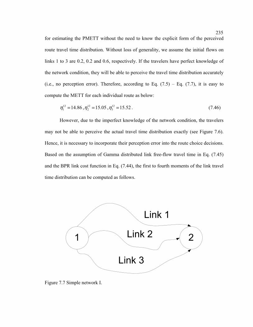
235for estimating the PMETT without the need to know the explicit form of the perceived

route travel time distribution. Without loss of generality, we assume the initial flows on

links 1 to 3 are 0.2, 0.2 and 0.6, respectively. If the travelers have perfect knowledge of

the network condition, they will be able to perceive the travel time distribution accurately

(i.e., no perception error). Therefore, according to Eq. (7.5) – Eq. (7.7), it is easy to

compute the METT for each individual route as below:

121 14.86η = , 12

2 15.05η = , 123 15.52η = . (7.46)

However, due to the imperfect knowledge of the network condition, the travelers

may not be able to perceive the actual travel time distribution exactly (see Figure 7.6).

Hence, it is necessary to incorporate their perception error into the route choice decisions.

Based on the assumption of Gamma distributed link free-flow travel time in Eq. (7.45)

and the BPR link cost function in Eq. (7.44), the first to fourth moments of the link travel

time distribution can be computed as follows.

Figure 7.7 Simple network I.

236 [ ]1 11.07E T = , [ ]2 9.05E T = , [ ]3 10.54E T = ;

21( ) 126.50E T⎡ ⎤ =⎣ ⎦ , 2

2( ) 91.08E T⎡ ⎤ =⎣ ⎦ , 23( ) 117.76E T⎡ ⎤ =⎣ ⎦ ;

31( ) 1492.45E T⎡ ⎤ =⎣ ⎦ , 3

2( ) 1007.93E T⎡ ⎤ =⎣ ⎦ , 33( ) 1390.10E T⎡ ⎤ =⎣ ⎦ ;

41( ) 18153.40E T⎡ ⎤ =⎣ ⎦ , 4

2( ) 12167.70E T⎡ ⎤ =⎣ ⎦ , 4( ) 17288.94aE T⎡ ⎤ =⎣ ⎦ .

Then, according to Eq. (7.18) – Eq. (7.21), the first to fourth moments of the

perceived travel time distribution can be computed as below:

1 11.07E T⎡ ⎤ =⎣ ⎦ , 2 9.05E T⎡ ⎤ =⎣ ⎦ , 3 10.54E T⎡ ⎤ =⎣ ⎦ ;

21( ) 128.72E T⎡ ⎤ =⎣ ⎦ , 2

2( ) 92.89E T⎡ ⎤ =⎣ ⎦ , 2( ) 119.87aE T⎡ ⎤ =⎣ ⎦ ;

31( ) 1568.36E T⎡ ⎤ =⎣ ⎦ , 3

2( ) 1062.58E T⎡ ⎤ =⎣ ⎦ , 33( ) 1460.75E T⎡ ⎤ =⎣ ⎦ ;

41( ) 19959.52E T⎡ ⎤ =⎣ ⎦ , 4( ) 13388.14aE T⎡ ⎤ =⎣ ⎦ , 4( ) 18971.19aE T⎡ ⎤ =⎣ ⎦ .

Consequently, according to Eq. (7.25), the first to fourth cumulants of the perceived link

travel time distribution can be derived as:

( )11 11.07κ = , ( )1

2 9.05κ = , ( )13 10.54κ = ;

( )21 6.26κ = , ( )2

2 10.92κ = , ( )23 8.77κ = ;

( )31 5.39κ = , ( )3

2 23.79κ = , ( )33 12.43κ = ;

( )41 7.29κ = , ( )4

2 78.39κ = , ( )43 26.91κ = .

Since the routes and links are identical in this special example, according to Eq. (7.26),

we have

( )( ) ( )12 i ip aκ κ= , 1, 2,3; 1,2,3,4a p i∀ = = = .

237By considering Eq. (7.30) and Eq. (7.31), the skewness and kurtosis of the perceived

route travel time distribution can be derived as:

1 0.34S = , 2 0.66S = , 3 0.48S = ;

1 0.19K = , 2 0.66K = , 3 0.35K = .

Based on the Cornish-Fisher (1937) Asymptotic Expansion in Eq. (7.27), the perceived

travel time budget (PTTB) can be estimated as:

( )121 0.9 14.35ξ = , ( )12

2 0.9 13.45ξ = , ( )121 0.9 14.45ξ = .

Then, by adopting Eq. (7.33), we can finally obtain the PMETT of each route

( )121 0.9 15.77η = , ( )12

2 0.9 15.61η = , ( )123 0.9 16.24η = . (7.47)

Analysis of the PMETT. Second, we examine the characteristics of the PMETT.

According to the definition of the PMETT, it can be decomposed into three different

components, i.e., the perceived mean travel time (PMTT), the perceived buffer time

(PBT), and the “perceived expected delay” (PED). This can be demonstrated more clearly

in Figure 7.8. Here, the “perceived expected delay” describes the impacts from the

unreliability aspect of travel time variability on travelers’ route choice decisions, and the

summation of the other two components (PMTT and PBT) gives the PTTB that

represents the travel time reliability requirement.

From the figure, we can see that travelers on route 3 may experience a higher

expected delay than those on route 1 when the 10% worse cases happened (i.e., (1-α)

quantile of worse travel times in the distribution tail), even though these two routes has

similar TTB. These worse cases may be due to various sources, such as severe incidents,

238

04

812

16

Route 1

Route 2

Route 3

M i n u t e s

PED

2.16

1.42

1.79

4.4

11.07

9.05

10.54

3.91

3.28

PTTB

)PMTT=

PMETT

+ ( PBT+

16.24

15.61

15.77

Figure 7.8 Analysis of the characteristics of PMETT.

bad weather conditions and special events. Therefore, for travelers who are concerned

with not only the travel time reliability, but also the unreliability of encountering worse

travel times, they may prefer route 1 than route 3, which has a lower METT.

The impacts on travelers’ route choice decision by considering both travel time

reliability and unreliability can be further illustrated in Figure 7.9. It shows the

percentages of each component (i.e., PMTT, PBT, and PED) corresponding to the

PMETTs. From the figure, we can see that the unreliability aspect of travel time

variability is as significant as the reliability aspect on travelers’ route choice decision.

Here, the PEDs (represents unreliability aspect) occupy 9%, 14% and 11%, respectively,

on the three routes. Furthermore, the results show that the sum of the reliability and

unreliability aspects has nearly 30% – 42% impacts on travelers’ route choice decisions

239

21%

70%

9%28%

14%

58%

24%11%

65%PMTT PMTT

PED

PBTPBT

PBT

PMTTRoute 2

PED PED

Route 3Route 1

Figure 7.9 Proportion of each component in the PMETTs. under an uncertain environment. Therefore, both reliability and unreliability aspects of

travel time variability should be considered in the route choice model.

Effects of the perception error. Third, we analyze the effects of the perception

error. Initially, we compare the equilibrium results of the METE and SMETE models.

The results are shown in Table 7.1. The column named ‘Route Flow’ gives the

equilibrium route flow pattern of each model. The METT and PMETT columns provide

the METT and the PMETT based on the equilibrium route flow pattern of each model,

respectively. For example, the PMETT column of the METE model provides the PMETT

of each route under the equilibrium route flows of the METE model given the same

perception error distribution adopted in the SMETE model. Similarly, the METT column

of the SMETE model shows the METT of each route under the computed equilibrium

route flows of the SMETE model given no perception error. To check the validity of the

results, we examine two conditions for each model: travel demand conservation

constraints and equilibrium conditions. As expected, both conditions are satisfied: the

route flows sum up to the OD travel demands and the corresponding equilibrium

measures (METT for the METE model and PMETT for the SMETE model) of all used

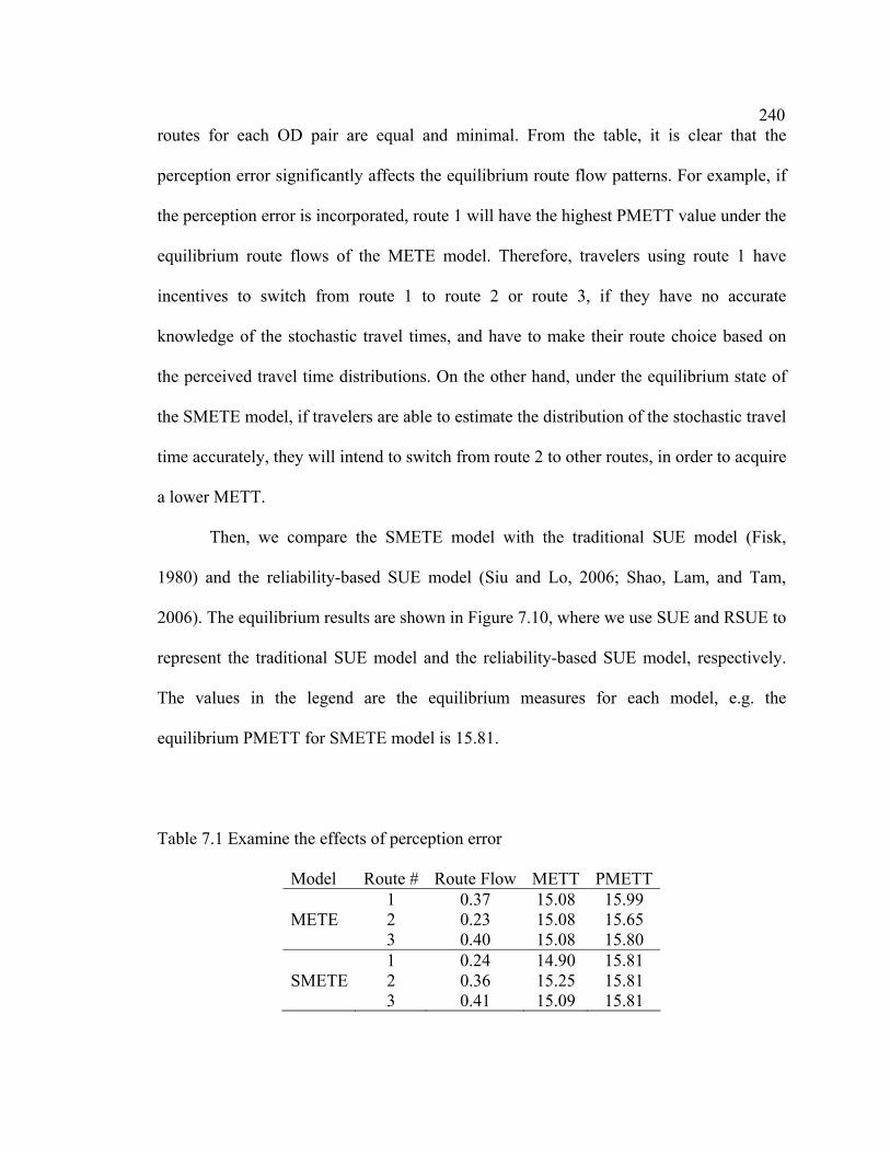
240routes for each OD pair are equal and minimal. From the table, it is clear that the

perception error significantly affects the equilibrium route flow patterns. For example, if

the perception error is incorporated, route 1 will have the highest PMETT value under the

equilibrium route flows of the METE model. Therefore, travelers using route 1 have

incentives to switch from route 1 to route 2 or route 3, if they have no accurate

knowledge of the stochastic travel times, and have to make their route choice based on

the perceived travel time distributions. On the other hand, under the equilibrium state of

the SMETE model, if travelers are able to estimate the distribution of the stochastic travel

time accurately, they will intend to switch from route 2 to other routes, in order to acquire

a lower METT.

Then, we compare the SMETE model with the traditional SUE model (Fisk,

1980) and the reliability-based SUE model (Siu and Lo, 2006; Shao, Lam, and Tam,

2006). The equilibrium results are shown in Figure 7.10, where we use SUE and RSUE to

represent the traditional SUE model and the reliability-based SUE model, respectively.

The values in the legend are the equilibrium measures for each model, e.g. the

equilibrium PMETT for SMETE model is 15.81.

Table 7.1 Examine the effects of perception error

Model Route # Route Flow METT PMETT 1 0.37 15.08 15.99 METE 2 0.23 15.08 15.65 3 0.40 15.08 15.80 1 0.24 14.90 15.81 SMETE 2 0.36 15.25 15.81 3 0.41 15.09 15.81

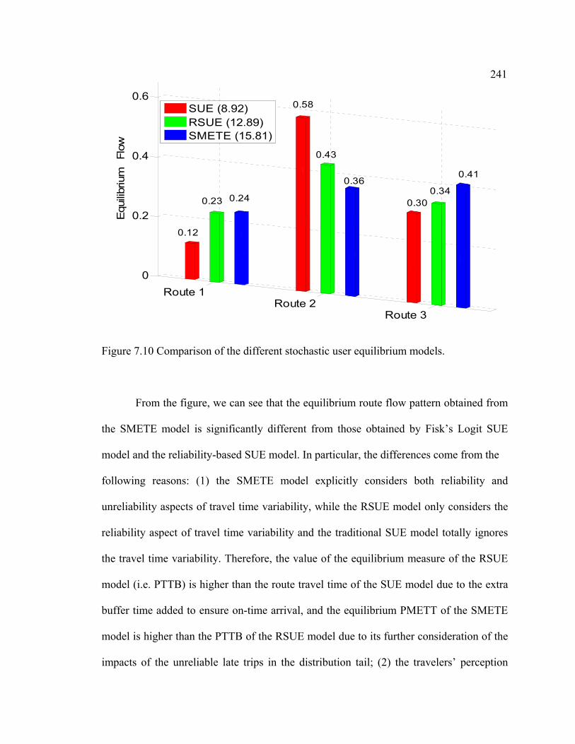
241

Route 1Route 2

Route 3

0

0.2

0.4

0.6

Equ

ilibr

ium

Fl

owSUE (8.92)RSUE (12.89)SMETE (15.81)

0.58

0.23 0.24

0.12

0.43

0.36

0.300.34

0.41

Figure 7.10 Comparison of the different stochastic user equilibrium models.

From the figure, we can see that the equilibrium route flow pattern obtained from

the SMETE model is significantly different from those obtained by Fisk’s Logit SUE

model and the reliability-based SUE model. In particular, the differences come from the

following reasons: (1) the SMETE model explicitly considers both reliability and

unreliability aspects of travel time variability, while the RSUE model only considers the

reliability aspect of travel time variability and the traditional SUE model totally ignores

the travel time variability. Therefore, the value of the equilibrium measure of the RSUE

model (i.e. PTTB) is higher than the route travel time of the SUE model due to the extra

buffer time added to ensure on-time arrival, and the equilibrium PMETT of the SMETE

model is higher than the PTTB of the RSUE model due to its further consideration of the

impacts of the unreliable late trips in the distribution tail; (2) the travelers’ perception

242error in the SMETE model depends on the distribution of the stochastic travel time. But

in the SUE and RSUE models, the perception error is independent of the actual travel

time distribution, and is just considered as a separate term. In fact, comparing with the

SUE and RSUE models, our model gives much less traffic flow on route 2, even it has

the lowest mean route travel time. This is reasonable because the risk averse travelers

would avoid these routes with higher travel time variation, if the expected travel time

does not increase much. Therefore, the travelers would rather travel through route 1 and

route 2 to get a higher confidence of on-time arrival, and at the same time, to avoid the

possible delays that are excessively higher than the TTB in the (1-α) quantile of the

distribution tail.

Example II

In this experiment, we use a second example to analyze the impacts of demand

variation, confidence level, as well as the perception error variance on the proposed

SMETE model. This simple network is shown in Figure 7.11, which consists of 4 nodes,

5 links and 3 routes. Here the routes and links are no longer identical, and the route-link

relationship is shown in Table 7.2.

Figure 7.11 Simple network II.

243Table 7.2 Route-link relationship of the test network

Route # Link Sequence 1 1-2 2 1-3-5 3 4-5

Table 7.3 Link characteristics

Statistical measure of the link free-flow travel times ( 0

at ) (min) Link # Mean Variance

Capacity ( aC ) (veh/min)

1 2 5 600 2 8 9 400 3 2 1 400 4 5 3 400 5 5 3 600

There is one OD pair (1, 4) with a demand of 1000 units. The mean and variance

of the free-flow travel time and capacity for each link in the test network are listed in

Table 7.3, and the corresponding route characteristics are listed in Table 7.4.

Analysis of the variations of demand level and confidence level. In the following,

we examine the effect of various combinations of demand level and confidence level.

Based on the discussions in the previous sections, it is reasonable to assume that all

travelers are risk-averse under an uncertain environment. Therefore, we only consider the

situation that the travelers' confidence level 50%α ≥ . Without loss of generality, we test

the confidence level from 0.6 to 0.99, and the demand level from 1 to 20 that represent

the OD demand increasing from 500 to 2400 with an interval of 100. Here, we assume

the perception error distribution of a unit travel time follows ( )0,0.1N . For

244Table 7.4 Route characteristics

Statistical measure of the route free-flow travel times ( 0

at ) (min) Route # Mean Variance

1 10 14 2 9 9 3 10 6

demonstration purpose, we only show the surface of the equilibrium PMETT in Figure

7.12.

From the figure, it is clear that the PMETT increases as the demand level

increases. Due to the congestion effect, the PMETT has a higher rate of increase at the

higher demand levels than that at the lower demand levels. This implies that the

consideration of both reliability and unreliability aspects of travel time variability may

have a more significant impact on travelers' route choice decision under heavier

congestion levels. At the same time, the price for maintaining the travel time reliability

requirement and avoiding the unreliability impacts is also higher. For example, knowing

that the congestion is severe, travelers have to depart earlier to ensure more frequent on-

time arrival and to minimize the associated risk of encountering excessively high delay.

Furthermore, we can see that the equilibrium PMETT is increasing while the confidence

level increases. This is to be expected since travelers need to budget extra time in order to

satisfy a higher travel time reliability requirement given by the increasing α value.

Analysis of the variations of perception error. Finally, we investigate the impacts

of the variations of perception error. Here, the OD demand is fixed at 1000, confidence

level is 90%, and the variance 2σ of the perception error distribution (N(µ, σ2)) of a unit

travel.

245

510

15

20

0.50.60.70.80.9

15

20

25

30

35

DL = 20, α = 0.99, PMETT = 38.48

DL = 13, α = 0.8, PMETT = 20.66

Figure 7.12 Equilibrium results under various demand-confidence level combinations. time increases from 0.1 to 1 with an interval of 0.1. The equilibrium PMETTs are

presented in Figure 7.13. From the figure, we can see that the PMETT increases as the

variance of the perception error increases. This is to be expected because high variance

of the perception error implies a larger variance of the perceived travel time distribution.

Therefore, in order to reach the specified travel time reliability requirement and to avoid

unacceptable delay, higher PTTB as well as PMETT are required.

246

0.1 0.7 1.3 1.9 2.6 3.1

20

21

22

P e r c e p t i o n E r r o r V a r i a n c e

P M

E T

T

Figure 7.13 Analysis under different perception error distributions.

Conclusions and Future Research

In this study, a stochastic mean-excess traffic equilibrium (SMETE) model is

proposed. The new model explicitly accounts for both reliability and unreliability aspects

of travel time variability and perception errors within the travelers’ route choice decision

process. A approximation method based on moment analysis is developed to estimate the

perceived mean-excess travel time (PMETT). The proposed model is formulated as a

variational inequality (VI) problem, which describes the stochastic mean-excess traffic

equilibrium condition, where each and every traveler simultaneously attempts to

minimize individual PMETT. A route-based algorithm based on the modified alternating

direction method is adopted to solve the proposed model. Illustration examples with

simple small networks are also investigated to highlight the essential ideas of the

proposed model and demonstrate the solution procedure.

247In order to facilitate the presentation of the essential ideas, we only consider one

user class in this study. Further extensions could be to consider multiple user classes with

various risk preferences or perception errors. Furthermore, more efficient algorithms for

finding the nonadditive PMETT route and solving the proposed SMETE model need to

be developed and tested on larger scale networks. Finally, the SMETE model can be

incorporated into network design problems (NDP) as a fundamental component of high

level transportation system risk assessment framework.

References

Abdel-Aty, M., R. Kitamura, and P. Jovanis. 1995. Exploring route choice behavior using

geographical information system-based alternative routes and hypothetical travel time information input. Transportation Research Record 1493: 74-80.

Acerbi, C., and D. Tasche. 2002. On the coherence of expected shortfall. Journal of

Banking and Finance 26(7): 1487-1503. Bernstein, D., and S. A. Gabriel. 1997. Solving the nonadditive traffic equilibrium

problem, p. 72-102. In P. M. Pardalos, D. W. Hearn, and W. W. Hager (Ed.). Network Optimization, Springer, New York.

Brownstone, D., A. Ghosh, T. F. Golob, C. Kazimi, and D. V. Amelsfort. 2003. Drivers’

willingness-to-pay to reduce travel time: Evidence from the San Diego I-15 congestion pricing project., Transportation Research Part A 37(4): 373-387.

Cambridge Systematics, Inc., Texas Transportation Institute, University of Washington,

Dowling Associates. 2003. Providing a highway system with reliable travel times. NCHRP Report No. 20-58[3], Transportation Research Board, National Research Council, U.S.A.

Chen, A., and Z. Ji. 2005. Path finding under uncertainty. Journal of Advanced

Transportation 39(1): 19-37. Chen, A., H. K. Lo, and H. Yang. 2001. A self-adaptive projection and contraction

algorithm for the traffic assignment problem with path-specific costs. European Journal of Operational Research 135: 27-41.

248Clark, S. D., and D. Watling. 2005. Modelling network travel time reliability under

stochastic demand. Transportation Research Part B 39(2): 119-140. Cornish, E. A., and R. A. Fisher. 1937. Moments and cumulants in the specification of

distributions. Extrait de la Revue de l'Institute International de Statistique 4, 1-14. de Palma, A., and N. Picard. 2005. Route choice decision under travel time uncertainty.

Transportation Research Part A 39: 295-324. Dial, R. B. 1971. A Probabilistic Multipath Traffic Assignment Algorithm Which

Obviates Path Enumeration. Transportation Research 5: 83-111. Facchinei, F., and J. S. Pang. 2003. Finite-Dimensional Variational Inequalities and

Complementarity Problems I, Springer, New York. 728 p. Fisk, C. 1980. Some developments in equilibrium traffic assignment. Transportation

Research Part B 14: 243-255. Fan, Y. Y., and Y. Nie. 2006. Optimal routing for maximizing the travel time reliability.

Networks and Spatial Economics 6(3): 333-344. FHWA. 2006. Travel time reliability: Making it there on time, all the time. Report No.

70, Federal Highway Administration. Gabriel, S. A., and D. Bernstein. 1997. The traffic equilibrium problem with nonadditive

path costs. Transportation Science 31(4): 337-348. Han, D. 2002. A modified alternating direction method for variational inequality

problems. Applied Mathematics and Optimization 45: 63-74. Liu, H., W. Recker, and A. Chen. 2004. Uncovering the contribution of travel time

reliability to dynamic route choice using real-time loop data. Transportation Research Part A 38: 435-453.

Lo, H. K., and A. Chen. 2000. Traffic equilibrium problem with route-specific costs:

Formulation and algorithms. Transportation Research Part B 34: 493-513. Lo, H. K., X. W. Luo, and B. W. Y. Siu. 2006. Degradable transport network: Travel

time budget of travelers with heterogeneous risk aversion. Transportation Research Part B 40: 792-806.

Lo, H. K., and Y. K. Tung. 2003. Network with degradable links: Capacity analysis and

design. Transportation Research Part B 37: 345-363.

249Mirchandani, P., and H. Soroush. 1987. Generalized traffic equilibrium with probabilistic

travel times and perceptions. Transportation Science 21: 133-152. Noland, R. B. 1999. Information in a two-route network with recurrent and non-recurrent

congestion, p. 95-114. In R. Emmerink and P. Nijkamp (Ed.). Behavioural and Network Impacts of Driver Information Systems, Ashgate, Aldershot, UK.

Noland, R., and K. A. Small. 1995. Travel time uncertainty, departure time choice, and

the cost of morning commutes. Transportation Research Record 1493: 150-158. Noland, R. B., K. A. Small, P. M. Koskenoja, and X. Chu. 1998. Simulating travel

reliability. Regional Science & Urban Economics 28: 535-564. Oppenheim, N. 1995. Urban travel demand modeling, John Wiley & Sons, New York.

480 p. Shao, H., W. H. K. Lam, Q. Meng, and M. L. Tam. 2006. Demand driven travel time

reliability-based traffic assignment problem. Transportation Research Record 1985: 220-230.

Shao, H., W. H. K. Lam, and M. L. Tam. 2006. A reliability-based stochastic traffic

assignment model for network with multiple user classes under uncertainty in demand. Network and Spatial Economics 6: 173-204.

Shao, H., W. H. K. Lam, M. L. Tam, and X. M. Yuan. 2008. Modeling rain effects on

risk-taking behaviors of multi-user classes in road network with uncertainty. Journal of Advanced Transportation 42(3): 265-290.

Sheffi, Y. 1985. Urban transportation networks: Equilibrium analysis with mathematical

programming methods. Prentice-Hall, Englewood Cliffs, New Jersey. 399 p. Small, K. A. 1982. The scheduling of consumer activities: Work trips. American

Economic Review 72(3): 467-479. Small, K. A., R. Noland, X. Chu, and D. Lewis, 1999. Valuation of travel-time savings

and predictability in congested conditions for highway user-cost estimation. NCHRP Report No. 431, Transportation Research Board, National Research Council, U.S.A.

Siu, B., and H. Lo. 2006. Doubly uncertain transport network: Degradable link capacity

and perception variations in traffic conditions. Transportation Research Record 1964: 59-69.

250Siu, B. W. Y., and H. K. Lo. 2007. Travel time budget and schedule delay costs under

uncertainty. Presented at the 3rd International Symposium on Transportation Network Reliability (INSTR), July 18-22, Delft, The Netherlands.

Stoer, J., and R. Bulirsch. 2002. Introduction to numerical analysis (3rd ed.), Springer,

New York. 752 p. Uchida, T., and Y. Iida. 1993. Risk assignment: A new traffic assignment model

considering the risk travel time variation. p. 89-105. In C. F. Daganzo (Ed.). Proceedings of the 12th International Symposium on Transportation and Traffic Theory, Amsterdam.

Wardrop, J. 1952. Some theoretical aspects of road traffic research. Proceedings of the

Institute of Civil Engineerings, Part II, 1: 325-378. Watling, D. 2006. User equilibrium traffic network assignment with stochastic travel

times and late arrival penalty. European Journal of Operational Research 175: 1539-1556.

van Lint, J. W. C., H. J. van Zuylen, and H. Tu. 2008. Travel time unreliability on

freeways: Why measures based on variance tell only half the story. Transportation Research Part A 42(1): 258-277.

Zhou, Z., A. Chen, and D. Han. 2007. An extended alternating direction method for

variational inequalities with linear equality and inequality constraints. Applied Mathematics and Computation 184(2): 769-782.

251CHAPTER 8

CONCLUSIONS AND RECOMMENDATIONS

In this chapter, the research in the previous chapters is concluded and the major

contributions of the dissertation are pointed out. The limitations of the research and a few

recommendations for future research are also provided.

Conclusions

Optimal path finding and traffic equilibrium problems are two fundamental and

interrelated problems in transportation, in which the travelers’ route choice behaviors and

risk preferences are inherently incorporated. They are the core of many surface

transportation applications encountered by transportation professionals on a daily basis.

Recent empirical studies on the value of time and reliability reveal that travel time

variability, which is considered as a risk to travelers making a trip, plays an important

role on travelers' route choice decision process. That is, travelers are not only interested

in saving their travel time but also in reducing their risk at the same time when making

their route choice decisions. Therefore, the objective of this dissertation is to develop

models and algorithms for addressing travel time variability with applications from

optimal path finding and traffic equilibrium problems.

Typically, the risk from travel time variability can be represented by two different

aspects: acceptable risk and unacceptable risk. Acceptable risk refers to the reliability

aspect of acceptable travel time, which is defined as the average travel time plus the

acceptable additional time (or buffer time) needed to ensure more frequent on-time

252arrivals, while unacceptable risk refers to the unreliability aspect of unacceptable late

arrivals (though infrequent) that have a travel time excessively higher than the acceptable

travel time. By considering the reliability and unreliability aspects of travel time

variability, two new optimal path finding models, i.e., the α-reliable path finding model

and the α-reliable mean-excess path finding model, and two new traffic equilibrium

models, i.e., the α-reliable mean-excess traffic equilibrium (METE) model and the

stochastic α-reliable mean-excess traffic equilibrium (SMETE) model, are proposed in

this study. Furthermore, the travelers’ perception error of the random travel time is also

incorporated into the SMETE model. The following conclusions are made in each chapter

of the dissertation.

In Chapter 1, a brief introduction of the research background and an outline of the

dissertation were given. Chapter 2 provided the fundamentals of the optimal path finding

problems and the traffic equilibrium problems. Chapter 3 proposed an adaptive α-reliable

path finding model, which is to adaptively determine a reliable path from a given origin

to a given destination under an uncertain environment, such that at each intermediate

node (including the origin) the desired reliability threshold α is satisfied and its

corresponding travel time budget (TTB) is minimum. The adaptive α-reliable path

finding model has the ability to incorporate both travelers' anticipation and real-time

traffic information into the route choice decision process. It provides travelers more

flexibility to better arrange their schedule and activities. That is, during the traveling

period, the more accurate estimation of their travel time budget can be acquired, and

travelers’ route strategy can be dynamically adjusted. The problem was formulated as a

chance constrained model, where the chance constraint represents the travel time

253reliability requirement under dynamic programming framework. The properties of the

proposed adaptive α-reliable path finding model were explored in relation with the

stochastic on-time arrival path finding model. Then, a discrete-time solution algorithm

was developed for finding the adaptive α-reliable path. The algorithm was successfully

applied on a real-size network. Chapter 4 proposed an α-reliable mean-excess model for

finding optimal path in stochastic networks. By using the new optimal path finding

criterion, i.e. the mean-excess travel time (METT), which was defined as the conditional

expectation of the travel time exceeding the TTB, this new model is able to account for

not only the reliability aspect that the traveler wishes to arrive at his destination within

the TTB, but also the unreliability aspect of encountering worst travel times beyond the

TTB. The model is useful for practical uncertain environments, where the travel time

distributions are generally nonnegative, asymmetric with long tails. The proposed model

is formulated as a stochastic mixed-integer nonlinear programming. To solve this difficult

problem, a double-relaxation scheme is developed to find the α-reliable mean-excess

path. A 9-nodes small network and a medium-size network (Sioux Falls network) were

adopted to demonstrate the features of the proposed model and the validity and efficiency

of the solution procedure. The flexibility of the model and the efficiency of the solution

procedure enable a fast and reliable path finding, which can be adopted in various real

world applications, such as the route guidance systems in ATIS. Chapter 5 presented a

mean-excess traffic equilibrium (METE) model. By adopting the METT as the route

choice criterion, the new model incorporates both reliability and unreliability concerns of

travel time variability of the travelers, and simultaneously addresses both questions: "how

much time do I need to allow?" and "how bad should I expect from the worse cases?"

254Therefore, it is able to capture the travelers’ risk preferences more completely and

accurately, and better reflect the travelers’ route choice decision processes. The new

model is described in a generic way, which allows flexible travel time distributions, and

formulated as a variational inequality (VI) problem. Qualitative properties of the model,

including the equivalence and the solution existence, were also rigorously proved. A

solution approach incorporating a projection-based algorithm was suggested for solving

the METE model. A small network and a medium-size network (Sioux Falls network)

were presented to demonstrate the model and the algorithm. Chapter 6 provided a

comparative analysis of three user equilibrium models under travel time variability (i.e.,

the traditional user equilibrium (UE) model, the demand driven travel time reliability-

based user equilibrium (DRUE) model, and the METE model), where the travel time

variability was assumed to come from the day-to-day travel demand fluctuation. The

METT was analytically derived, which reveals the relationships among the three different

route choice criteria adopted in the three user equilibrium models for the comparative

analysis conducted in this study. The limited numerical results showed that the three

models are indeed different and highlighted the essential ideas of the METE model.

Chapter 7 presented a novel stochastic α-reliable mean-excess traffic equilibrium

(SMETE) model. As an extension of the METE model, the travelers' perception error is

also incorporated into this model in addition to considering of both reliability and

unreliability aspects of travel time variability. Furthermore, the distribution of the

perception error is assumed to depend on the actual distribution of the random travel

time. Therefore, the travelers’ route choice decisions are based on the perceived travel

time distribution, which is composed of both distributions of the probabilistic travel time

255and the perception error. Due to the difficulty of obtaining the analytical from of the

perceived travel time distribution, a moment analysis-based approximation approach was

proposed to estimate the perceived mean-excess travel time (PMETT). The SMETE

model is formulated as a VI problem, which describes the conditions that govern the

SMETE state, where each and every traveler simultaneously attempts to minimize

individual PMETT. A route-based algorithm based on the modified alternating direction

method was developed to solve the SMETE model. Illustrative examples with simple

small networks were also investigated to highlight the essential ideas of the proposed

model, and to demonstrate the approximation approach and the solution procedure.

Contributions

Due to the importance of optimal path finding and traffic equilibrium problems in

the transportation field and the increasing interests on studying the travelers’ route choice

decision under uncertain environments, this dissertation developed new optimal path

finding and traffic equilibrium models by incorporating various aspects of travel time

variability into the route choice consideration. The novel models and algorithms

presented in this dissertation are expected to provide the following important

contributions:

1. The development of the adaptive α-reliable path finding problem based on the

investigation of the reliability aspect of travel time variability. The new model is able

to adaptively determine an optimal path under an uncertain environment, such that

both travelers' anticipation and real-time traffic information can be incorporated into

the travelers’ route choice decision process. The problem is formulated as a chance

256constrained model, where the chance constraint represents the travel time reliability

requirement under a dynamic programming framework. The properties of the

proposed adaptive α-reliable path finding model are rigorously examined in relation

with the stochastic on-time arrival path finding model. Therefore, a discrete-time

solution algorithm can be developed and applied in a real size network.

2. The development of the α-reliable mean-excess path finding model under the

exploration of both reliability and unreliability aspects of travel time variability. A

new optimal path finding index (i.e, METT) is proposed, which is able to capture the

travelers’ risk preferences more completely and accurately. A double-relaxation

solution procedure is developed to solve the stochastic mixed-integer nonlinear

programming formulation of the model.

3. The development of the METE model, where METT is adopted as the new route

choice criterion. Therefore, the new model is able to incorporate both reliability and

unreliability aspects of travel time variability and better reflect the travelers’ route

choice decision process in a network equilibrium framework. The model is

formulated as a VI problem and its qualitative properties are rigorously proved. A

route-based solution procedure based on a projection-based algorithm is suggested to

solve the proposed model.

4. The comparison among three different traffic equilibrium models (UE, DRUE,

METE) on stochastic network. The analytical form of the METT is derived, where

the travel time variability is introduced by day-to-day travel demand fluctuation. It

reveals the relationships among the three different route choice criteria adopted in

these three user equilibrium models. The limited numerical results show that the three

257models are indeed different and highlighted the essential ideas of the METE model.

5. The development of the SMETE model, where both reliability and unreliability

aspects of travel time variability, and traveler’s variable perception errors are all

explicitly incorporated into a unified network equilibrium framework. A moment

analysis-based approximation approach is proposed, which enables the estimation of

PMETT without knowing the closed form of the perceived travel time distribution.

Finally, a route-based algorithm based on the modified alternating direction method is

developed to solve the proposed model.

Limitations

This research has made several significant contributions, but there are some

limitations that can be listed as below:

1. In the adaptive α-reliable path finding model, the link travel time distributions are

assumed to be independent. However, the link travel times could be correlated in

practice. For example, in a transportation network, if the level of service of one link is

affected, it is very likely that the adjacent links are also affected.

2. In general, the double-relaxation algorithm proposed for solving the α-reliable mean-

excess path finding model is a heuristic approach. Therefore, the solution could be

sub-optimal. In addition, the computational complexity of the algorithm has not been

rigorously analyzed.

3. In this study, the new traffic equilibrium models are proposed under a generic form,

where the travel time variability was assumed to be exogenously defined by the

system to facilitate the numerical experiments. In practice, the stochastic travel time

258variation may be introduced by various sources either exogenously or endogenously.

4. In the comparitive study, the random travel demands among the OD pairs are

assumed to be independent. In reality, the OD demands could be correlated.

5. Though the limited numerical results demonstrate the difference among the proposed

and the existing traffic equilibrium models, due to the complex situations in the real

world, no one model is sufficient in capturing all aspects of the travelers’ risk-taking

behavior in the route choice decision process, and which model is the most realistic is

an open question.

6. The models proposed in this dissertation are assumed for a single user class and fixed

demand. In reality, there could be multiple user classes and the travel demand could

depend on the congestion level.

Recommendations for Future Research

There are some recommendations for future research of the optimal path finding

and traffic equilibrium problems on stochastic networks:

1. The adaptive α-reliable path finding problem presented in Chapter 3 could be

extended by incorporating link correlation to capture dependences on multiple links.

2. The computation complexity of the double-relaxation algorithm in Chapter 4 could be

rigorously analyzed to obtain insights for future improvement. In additional, more

larger networks should be used to study the efficiency of the algorithm.

3. It is attractive to consider various sources of travel time variability, such as random

link capacity degradation, weather, incidents and work zone, with the modeling

scheme proposed in this dissertation.

2594. The comparison of the different traffic equilibrium models under stochastic travel

demand in Chapter 6 could be generalized by incorporating OD demand correlation.

5. The new traffic equilibrium models presented in Chapter 5 and Chapter 7 could be

further extended to consider multiple user classes, whose risk-taking behaviors are

different. Furthermore, the travel demand in the traffic equilibrium problems could be

elastic. That is, the demand will be a non-increasing function of the corresponding

level-of-service.

6. From the computational point of view, more efficient algorithms need to be

developed to find the nonadditive (perceived) mean-excess travel time routes within

the network equilibrium framework. Furthermore, these algorithms need to be tested

on larger networks.

7. Given that there are different equilibrium models under uncertainty, which model is

the most realistic is an open question. Thus, it is worthwhile to conduct empirical

studies to examine this open question.

260

APPENDIX

261Co-Editor-In-Chief Journal of Advanced Transportation Department of Civil Engineering The University of Calgary Calgary, Alberta Canada T2N 1N4 Dear Editor, I am preparing my dissertation in the Department of Civil & Environmental Engineering at Utah State University. I hope to complete me degree in the Spring of 2008. An article, Comparative analysis of three user equilibrium models under stochastic demand, of which I am first author, and which will appear in your journal Journal of Advanced Transportation 42 (3): 265 – 290. reports an essential part of my dissertation research. I would like permission to reprint it as a chapter in my dissertation (Reprinting the chapter may necessitate some revision.) Please note that USU sends dissertations to Bell & Howell Dissertation Services to be made available for reproduction. I will include the copyright and permission information in a special appendix. If you would like a different way of acknowledgment, please so indicate. Please indicate your approval of this request by signing in the space provided, and attach any other form necessary to confirm permission. If you charge a reprint fee for use of an article by the author, please indicate that as well. If you have any questions, please call me at the number below or send me an e-mail message. Thank you for your assistance. Zhong Zhou I hereby give permission to Zhong Zhou to reprint the requested article in his dissertation, with the following copyright and permission information: (Comparative analysis of three user equilibrium models under stochastic demand. Journal of Advanced Transportation 42 (3): 265 - 290.)

Signed Date March 21, 2008 Fee : NO FEE

262CURRICULUM VITAE

Zhong Zhou (May, 2008)

EDUCATION

Ph.D. Civil & Environmental Engineering May 2008

Utah State University (expected)

M. S. Computational Mathematics June 2000

Nanjing University, China

B. S. Computational Mathematics and Application Software July 1997

Nanjing University, China

PROFESSIONAL EXPERIENCE

• Co-instructor for the graduate level course CEE 6210: Transportation System Analysis,

Utah State University, (Spring, 2006)

• Research Assistant for the NSF project “An Integrated Transportation Network

Reliability Analysis Framework” sponsored by the National Science Foundation (NSF)

CAREER Award, Utah State University, (Sept. 2002 – Present)

• Software Designer and Developer for the project “Graphical User Interface of the Path

Flow Estimator” sponsored by the California Partners for Advanced Transit and Highway

(PATH) Program and Institute of Transportation Studies (ITS) at UC Irvine, Utah State

University (Aug. 2005 - June 2006)

• Software Engineering, START Corporation, China (July, 2000 – July, 2002)

• Project Assistant, Nanjing University, China (September, 1997 – July, 2000)

263 REFEREED JOURNAL PUBLICATIONS

• Zhou, Z., Chen, A., and Wong, S.C. (2007) Alternative formulations of a

combined trip generation, trip distribution, modal split, and trip assignment

model. European Journal of Operational Research (accepted).

• Zhou, Z . and Chen, A. (2008) Comparative analysis of three user equilibrium

models under stochastic demand. Special Issue of Journal of Advanced

Transportation: Evaluation and Enhancement of Transport Network Reliability:

Network Equilibrium Based Approach (accepted).

• Chen, A. and Zhou, Z. (2008) Solving the non-additive traffic equilibrium

problem with capacity constraints. Transportation Research, Part B:

Methodological (tentatively accepted).

• Chen, A., Kim, J., Zhou, Z., and Chootinan, P..(2008) Alpha reliable network

design problem. Transportation Research Record 2029: 49-57

• Zhou, Z., Chen, A., and Han, D. (2007) An extended alternating direction method

for variational inequalities with linear equality and inequality constraints. Applied

Mathematics and Computation, 184(2), 769-782.

• Zhou, Z. and Chen, A. (2003) A self-adaptive scaling technique embedded in the

projection traffic assignment algorithm. Journal of Eastern Asia Society for

Transportation Studies, Vol. 5, 1647-1662.

264REFEREED CONFERENCE PAPERS

• Chen, A., Zhou, Z., Chootinan, P. and Wong, S.C. (2008) A bi-objective reliable

network design model. Paper accepted for the 87th annual meeting of the

Transportation Research Board, Washington, D.C., USA.

• Chen, A., Kongsomsaksakul, S., Zhou, Z., Lee, M., and Recker, W. (2007)

Chapter 11: Assessing network vulnerability of degradable transportation

systems: An accessibility-based approach. In Proceedings of the 17th International

Symposium of Transportation and Traffic Theory(ISTTT17) (a peer reviewed

series since 1959), Elservier. Edited by M.G.H. Bell, B. Heydecker, and R.

Allsop, 236-262.

• Chen, A., Zhou, Z., Chootinan, P., and Wong, S.C. (2007) Optimizing capacity

reliability and travel time reliability in the network design problem. Proceedings

of the 12th Hong Kong Society of Transportation Studies Conference:

Transportation Systems: Engineering and Management, Hong Kong, P.R. China,

edited by C.H. Cheng, S.C. Ho and J.M.Y. Leung, 223-232.

• Chen, A., Chootinan, P., and Zhou, Z. (2007) Capacity reliability versus travel

time reliability in the network design problem. Proceedings of the 3rd

International Symposium on Transportation Network Reliability (INSTR07), 19-

20 July 2007, The Netherlands.

• Chen, A., Kongsomsaksakul, S., and Zhou, Z. (2007) Assessing network

vulnerability using a combined travel demand model. Paper presented at the 86th

265annual meeting of the Transportation Research Board, Washington, D.C., USA.

• Zhou, Z. and Chen, A. (2006) A self-adaptive gradient projection algorithm for

solving the nonadditive traffic equilibrium problem. Paper presented at the 85th

annual meeting of the Transportation Research Board, Washington, D.C., USA.

• Zhou, Z. and Chen, A. (2005) Traffic equilibrium problem: Incorporating traffic

restraint and random perception. Proceedings of the 10th Hong Kong Society of

Transportation Studies Conference: Transportation and the Economy, Hong

Kong, P.R. China, edited by W.H.K. Lam and J. Yan, 43-52.

• Zhou, Z. and Chen, A. (2003) Stochastic traffic equilibrium problem: a

comparison between length-based and congestion-based C-logit models,

Proceedings of the 8th Hong Kong Society of Transportation Studies Conference:

Transportation & Logistics, Hong Kong, P.R. China, edited by D. Becky P.Y.

Loo and Stephen W.K. Lam, 244-253.

SUBMITTED JOURNAL PAPERS

• Chen, A. and Zhou, Z. (2008) The α-reliable mean-excess traffic equilibrium

model with stochastic travel times. Transportmetrica.

• Zhou, Z. and Chen, A. (2008) The α-reliable mean-excess path finding model in

stochastic networks. Applied Mathematics and Optimization

266• Zhou, Z., Chen, A., and Behkor, S. (2007) C-logit stochastic user equilibrium

model: Formulations and solution algorithm. Transportation Research Part B:

Methodological (2nd review)

• Chen, A. and Zhou, Z. (2007) Modeling physical and environmental side

constraints in traffic equilibrium problem. Transportation Research, Part A:

Policy and Practice.

• Chen, A., Zhou, Z. and Lam, W.H.K. (2007) A stochastic a-reliable mean-excess

traffic equilibrium model with stochastic travel times and perception errors.

Abstract submitted to the 18th International Symposium of Transportation and

Traffic Theory.

• Zhou, Z. and Chen, A. (2007) Adaptive alpha-reliable path finding problem:

Formulation and solution algorithm. IEEE Transactions on Intelligent

Transportation Systems.