Modelling Vertical Plate Radiators for Electric ... · PDF fileModelling Vertical Plate...
71
Modelling Vertical Plate Radiators for Electric Transformers Efacec José Paulo Barbosa Baltazar Dissertação do MIEM Orientador na Efacec: Eng.º Hugo Campelo Orientador na FEUP: Prof. Clito Afonso Faculdade de Engenharia da Universidade do Porto Mestrado Integrado em Engenharia Mecânica Junho de 2014
-
Upload
duongquynh -
Category
Documents
-
view
224 -
download
2
Transcript of Modelling Vertical Plate Radiators for Electric ... · PDF fileModelling Vertical Plate...

Modelling Vertical Plate Radiators for Electric Transformers
Efacec
José Paulo Barbosa Baltazar
Dissertação do MIEM
Orientador na Efacec: Eng.º Hugo Campelo
Orientador na FEUP: Prof. Clito Afonso
Faculdade de Engenharia da Universidade do Porto
Mestrado Integrado em Engenharia Mecânica
Junho de 2014

Modelling Vertical Plate Radiators for Electric Transformers
ii
Acknowledgments
I would like to acknowledge my supervisors on this work, Prof. Clito Afonso at
the University and Eng.º Hugo Campelo at the company Efacec.
I would also like to thank my family, my friends and my girlfriend for all the
support, encouragement and patience given during the entire course of Mechanical
Engineering.

Modelling Vertical Plate Radiators for Electric Transformers
iii
Abstract
In the electric conversion process of a transformer, some power is lost and
converted into heat. These heat losses lead to temperature rises that have to be
controlled with cooling solutions, since working with high temperatures lead to the
deterioration of components and reduces the lifespan of the transformer. The coils and
core of a transformer are usually immersed in an oil filled tank. For large transformers
the oil is heated in this tank and then cooled in external heat exchangers. The typical
heat exchangers used consists in thin vertical plate radiators, in which the oil transfers
heat to the surrounding air.
The objective of this work was to create and evaluate calculation methodologies
to predict the cooling capacity of vertical plate radiators. The developed methodologies
use heat transfer correlations for oil and air in both natural and forced convection. For
air natural convection, preliminary experiments were performed and results were
compared with the calculation methodology using correlations from literature. The
correlations were also applied to other two case studies and proved to have low
accuracy on predicting the radiators cooling capacity. For air forced convection, CFD
simulations were performed and results were compared to the calculation methodology.
This comparison showed that the air flow between radiator’s plates is not fully
developed and that literature correlations do not take into account that phenomenon,
causing an underestimation of the cooling capacity by the calculation methodology.
New heat transfer correlations were developed for air forced convection using the CFD
simulation data, in order to improve the calculation methodology. These new
correlations presented great accuracy when applied to the radiators of a real transformer
(cooling capacity deviations of 3.9% relatively to results from tests performed by
Efacec company). The radiation heat transfer mode was included in the calculation
methodologies and results showed that this is an important mechanism in radiators,
especially when air convection is natural.
Modelling Vertical Plate Radiators for Electric Transformers
iv
Nomenclature
cp – specific heat at constant pressure [J/(kg.K)]
Dh – Hydraulic diameter [m]
F – View factor [-]
h – Convective heat transfer coefficient [W/(m2.K)]
k – Thermal conductivity [W/(m.K)]
L - Plate length [m]
– Mass flow rate [kg/s]
N – Number of plates per radiator [-]
Nu – Nusselt number [-]
P – Heat dissipation or cooling capacity [W]
Pr – Prandtl number [-]
Q – Volumetric flow rate [m3/s]
R – Thermal resistance [K/W]
Ra – Rayleigh number [-]
Re – Reynolds number [-]
S - Distance between plates [m]
T – Temperature [ºC]
v – Velocity [m/s]
W - Plate width [m]
- Hydrodynamic entry length [m]
β – Coefficient of volumetric thermal expansion [K-1
]
ε – Emissivity [-]
μ – Dynamic viscosity [Pa.s]
ν – Kinematic viscosity [m2/s]
ρ – Density [kg/m3]
σ – Stefan–Boltzmann constant [W.m-2
.K-4
]
Subscripts:
ave – Average
channel – Of one oil channel
conv - Convection
end – On the radiator outer surfaces

Modelling Vertical Plate Radiators for Electric Transformers
v
ext – External
fan – Quantity per fan
fd – Fully developed
gap – On the radiator inner surfaces
plate – Quantity per plate
in - Inlet
int – Internal
out – Outlet
rad - Radiation
radiator – Quantity per radiator
transformer – Total quantity for the transformer
wall – On the wall

Modelling Vertical Plate Radiators for Electric Transformers
vi
Table of Contents
1. Introduction ....................................................................................................... 1
1.1. Presentation of Efacec ................................................................................ 1
1.2. Transformers and Heat Generation ............................................................ 1
1.3. Project Description and Objectives ............................................................ 2
1.4. Structure and Organization ........................................................................ 4
2. Background ....................................................................................................... 5
2.1. Transformer Cooling States ....................................................................... 5
2.2. Vertical Plate Radiators.............................................................................. 6
2.3. State of Art ................................................................................................. 9
3. Modelling of Heat Exchangers ....................................................................... 16
3.1. Heat Transfer Modes Analysis – AN and AF .......................................... 16
3.2. Calculation Procedures – AN and AF ...................................................... 18
3.2.1. Convective Heat Transfer Inside the Oil ........................................... 18
3.2.2. ONAN and ODAN states .................................................................. 20
3.2.3. ONAF and ODAF states .................................................................... 23
3.2.4. Radiation............................................................................................ 25
3.3. CFD Simulations Methodology – AF ...................................................... 26
3.4. Experimental Details – AN ...................................................................... 31
4. Results and Discussion ................................................................................... 33
4.1. Air Forced Convection ............................................................................. 33
4.1.1. CFD Simulation Results .................................................................... 33
4.1.2. Formulation of New Correlations ...................................................... 40
4.1.3. Bottom vs. Side Ventilation .............................................................. 44
4.1.4. Transformer 546A in ONAF ............................................................. 47
4.2. Air Natural Convection ............................................................................ 49
4.2.1. Experimental Results ......................................................................... 49
4.2.2. Transformer 546A in ONAN............................................................. 52
4.2.3. Hyosung Experiments ....................................................................... 54
5. Conclusions and Future Work ........................................................................ 56
6. References ....................................................................................................... 58
Annex A: Oil and Air Properties ..................................................................... 59

Modelling Vertical Plate Radiators for Electric Transformers
vii
Annex B: Parameters of CFD Simulations ..................................................... 61
Annex C: Experiments Uncertainty Analysis ................................................. 63

Modelling Vertical Plate Radiators for Electric Transformers
1
1. Introduction
The first section of this chapter presents Efacec, the company where the work
was developed. The second section introduces transformers and contextualizes the heat
generation in this equipment. Then, after explaining the importance of cooling
transformers efficiently, the project was described along with its objectives. Finally, in
the last section is presented the organization of this work.
1.1. Presentation of Efacec
Efacec is a Portuguese company with business activity in the electric field, being
present in more than 65 countries in the five continents. This company provides systems
and solutions for the areas of energy, mobility and environment [1].
Design and manufacture of transformers is developed by Efacec, including
power and distribution Transformers (Figure 1). Distribution includes dry type and oil
immersed transformers, from 50 to 20000 kVA. Regarding power transformers, Efacec
produces Shell and Core types with rated powers up to 1500 and 350 MVA,
respectively. These two types differ in constructive aspects such as the coils’ shape, the
winding type and the magnetic core arrangement (vertical or horizontal).
Figure 1 – Examples of distribution (left) and power (right) transformers [1].
Efacec’s Research and Development Department analyses, among other subjects,
the electrical, magnetic and cooling behavior of transformers equipment in order to
improve their efficiency and build new solutions.
1.2. Transformers and Heat Generation
The function of transformers is to change voltage levels between two circuits,
being consequently modified the current values. Transformers have efficiency greater
than 99%l and consequently the input and output powers are nearly the same, being the
lost power converted to heat. Since power transformers operate with great power levels,
the heat losses will lead to temperature rise that have to be controlled by cooling [2].

Modelling Vertical Plate Radiators for Electric Transformers
2
Working with too high temperatures will deteriorate the winding insulation and the
transformer oil, which are two aspects in which the lifespan of a transformer is very
dependent [3]. This way it is very important to ensure an effective cooling system,
especially in situations where high power is involved.
Transformers usually use oil and air as internal and external cooling mediums,
respectively. When using oil, the coils and core are immersed in an oil filled tank. In
small transformers, the tank surface in contact with the exterior air is enough to provide
the heat dissipation needed. In larger transformers, since there is more heat generated, it
is required that the oil circulates from the transformer’s tank to external heat exchangers
[2]. In Figure 2, it can be seen a power transformer with external radiators attached.
Figure 2 – Efacec’s Power Transformer with radiators attached [1].
The oil and air circulation can be forced by mechanisms such as pumps and fans,
respectively, or can be driven by natural buoyance forces. Having these circulation
regimes, there will be forced and natural convection that can be combined together (for
example the oil can be driven naturally and air forced by fans).
1.3. Project Description and Objectives
One of the five targets that European Union established for 2020 concerns the
climate changes and the energy sustainability, more particularly an increase of 20% in
energy efficiency [4]. Regarding transformers, although they are optimized in terms of
the electric conversion process, there is still a lot of work that can be done in the cooling
procedures. The optimization of transformer’s cooling capacity allows the utilization of
more compact equipment and consequently the reduction in manufacturing materials.
Several researches and improvements have been performed in the interior of
transformers for enhance heat dissipation, being the analysis of the external heat
exchangers less explored. These apparatus are a fundamental component for dissipating
the heat generated into the exterior of a transformer. The capability of predicting the
behaviour and cooling capacity of heat exchangers leads to a better and more adequate

Modelling Vertical Plate Radiators for Electric Transformers
3
selection of equipment for each particular transformer. This knowledge would allow the
completion of a global system for designing transformers and also can lead to
modifications in heat exchangers configurations in order to enhance their cooling
capacity.
Consequently, the aim of this project is to develop and evaluate calculation
methods to predict the cooling capacity of a type of heat exchangers applied in
transformers: vertical plate radiators. These predictions should be based on the selection
of the known input data (such as the oil inlet temperature, radiator characteristics, etc.)
and on the calculation of the output parameters that are essentially the cooling capacity
and the oil outlet temperature. In Figure 3 is a scheme of oil cooling in a vertical plate
radiator and in Figure 4 is a diagram of the main calculation inputs and outputs.
Figure 3 – Scheme of oil cooling in radiator.
Figure 4 – Calculation inputs and outputs.
The mathematical model to be developed in this work is based on the utilization
of heat transfer correlations. These correlations use dimensionless numbers (such as
Reynolds, Rayleigh, Prandtl and Nusselt numbers), which in turn are calculated using
the properties of the fluids. This implies the utilization of iteration procedures, for

Modelling Vertical Plate Radiators for Electric Transformers
4
example the oil outlet temperature has an initial arbitrated value that is corrected by
progressive iterations.
Although results from experiments or CFD simulations can be more accurate
than calculation methods, the last one is a much faster and less expensive tool. Using
experimental apparatus to study every new configuration that appears would imply an
unfeasible cost and time. With simulation tools the time problem would still remain if
one wanted to study every single case.
In order to improve the calculation methodology, the existing correlations on
literature (for natural and forced convection) were studied and the results will be
compared with other sources in order to analyse the applicability of the correlations.
Also, for the air forced convection, some correlations were developed using CFD
simulations.
1.4. Structure and Organization
The text that follows the introduction is organized in four chapters. The first of
these chapters is the Background, where the nomenclature of the transformer cooling
states is presented, followed by the description of the type of radiators studied in this
work. The state of the art is presented at the last section of the Background, concerning
studies on vertical plate radiators by CFD simulations and experiments.
In chapter 3, the heat transfer modes on radiators are analysed. After this
analysis, the calculation procedures are presented with the respective assumptions and
then the methodology used to perform CFD simulations of air forced convection is
described. Preliminary experiments were conducted for air natural convection and are
described in the last section of chapter 3.
Chapter 4 contains the results and discussion divided into two sections: air
forced convection and air natural convection. For the forced convection, the results from
CFD simulations and its comparison with the calculation methodology using literature
correlations are presented. Then the formulation of new correlations based on CFD
results is shown, followed by a comparison between ventilate radiators with fans on the
side and on the bottom. The subsection Transformer 546A in ONAF presents a
comparison between the calculation procedures applied in a real transformer from
Efacec and data from operational tests performed by the company in the same
transformer.
For natural convection, the literature correlations were evaluated applying them
in three case studies: the preliminary experiments performed, a transformer from Efacec
and the experiments conducted by [5].
In the last chapter the final conclusions are presented and future work is
recommended.

Modelling Vertical Plate Radiators for Electric Transformers
5
2. Background
In this chapter, a background for the transformers external heat exchangers is
presented. A transformer can operate at different cooling states, which designation
depends on the cooling mediums used and their circulation mechanisms. The
nomenclature of the cooling states is presented in the first section. In the second section
the vertical plate radiators are described along with their geometrical characteristics and
main configurations. The state of art on the performance of the radiators is presented on
the last section of this chapter.
2.1. Transformer Cooling States
There are several cooling states used for the refrigeration of power transformers
and therefore transformers shall be identified according to the applied method.
According to the International Electrotechnical Commission (IEC), for the case of
liquid-immersed transformer, the cooling state is identified by a four letter code. The
first letter relates to the internal cooling medium and the second regards to its
circulation mechanism. The third and fourth letters are associated to the external cooling
medium and its circulation mechanism, respectively. The existing letters and their
meaning can be seen in Table 1 [6].
Table 1 - Four letter code to identify transformer’s cooling state [6]
Order Letter Meaning
First
O Mineral oil or synthetic insulating liquid with fire point less or
equal to 300ºC.
K Insulating liquid with fire point over 300ºC.
L Insulating liquid with no measurable fire point.
Second
N Natural thermosiphon flow through cooling equipment and in
windings.
F Forced circulation through cooling equipment, thermosiphon
flow in windings.
D Forced circulation through cooling equipment, directed from
the cooling equipment into at least the main windings.
Third A Air
W Water
Fourth N Natural convection.
F Forced circulation (fans or pumps).
A transformer can have alternative cooling states. For example, an
ONAN/ONAF has a set of fans which may be put into service at high loading [6].
Along this project, four types of cooling states were studied:
ONAN – Oil Natural Air Natural
ODAN – Oil Directed Air Natural
ONAF – Oil Natural Air Forced
ODAF – Oil Directed Air Forced

Modelling Vertical Plate Radiators for Electric Transformers
6
Oil immersion is commonly used because this cooling medium has higher
dielectric strength than air and that is fundamental to prevent electric breakdown or
discharge at the coils and core of the transformer [2]. Therefore it is not possible to
choose the internal cooling medium attending only to its cooling capacity, since it
works also as an electrical insulator.
The typical oils used in transformers are the mineral type ones. Mineral oils
provide efficient cooling and electrical insulation, but they have low biodegradability.
Due to this inconvenience, the main research that is being carried out has the aim of
finding other fluids that are biodegradable (like vegetable oil-based and synthetic esters)
and still have the required properties for operation. This kind of research and testing can
be found in [7] and [8].
Air is frequently chosen to be the external cooling medium, since it doesn’t
involve acquisition costs and its return to the environment doesn’t require special
attention. The same may not be true when using water.
Systems based on oil and air natural flows (ONAN – Oil Natural Air Natural)
are the most reliable ones, since there aren’t any mechanical components, like pumps or
fans, which can fail. This type of systems are absent of mechanical vibration and noise
[5] and their simplicity makes them economically interesting. On the other hand, forced
circulation of the cooling mediums brings more efficiency and from there results greater
cooling capacities and/or more compact equipment.
2.2. Vertical Plate Radiators
The typical heat exchangers used in power transformers consists in thin vertical
plate radiators. Figure 5, shows an example of this type of heat exchangers. There is a
great interest in using these radiators due to their construction simplicity that makes
them more economically sustainable.
Figure 5 - Vertical Plate Radiators [9].
A scheme of the oil circuit can be seen in Figure 6. The oil comes from the
transformer’s tank from the inlet pipes and enters in the radiator plates at their top. After

Modelling Vertical Plate Radiators for Electric Transformers
7
passing through the plates, the oil re-enters the tank through the outlet pipes located in
the bottom part of the radiators. At the external surface of the plates circulates air at
room temperature, driven by natural or forced circulation (for this last one are used
coupled fans).
Figure 6 – Oil circulation scheme.
Presently, the cooling capacity of the radiators is estimated using tabulated
experimental information and some correction factors are applied. There are several
parameters that affect the cooling capacity and some of them are not taken into account
in that method. The main geometrical parameters are presented in Table 2 and Figure 7.
Table 2 – Radiators geometrical parameters
Geometrical Parameter Range or Standard Values
Distance Between Plates - S 45 mm
Plate Width - W 520 mm
Plate Length - L 800 to 3500 mm
Figure 7 – Radiator and main dimensions. Adapted from [10].

Modelling Vertical Plate Radiators for Electric Transformers
8
The plates are evenly separated and all have the same width, but in the same
radiator can be present plates of different lengths. Each plate has six oil channels. In
Figure 8 is presented the geometry and dimensions of an oil channel cross section. This
geometry was designed in SolidWorks (Figure 9) in order to easily estimate values of
areas and perimeters.
Figure 8 – Oil channel cross section dimensions. [11]
Figure 9 – Oil channel cross section designed in SolidWorks software.
In order to predict the cooling capacity provided by the radiators installed in a
transformer and also the oil temperature at the radiators’ outlet, it is necessary to
consider other parameters beside the geometrical ones. Such parameters include:
The oil flow rate;
The air flow rate;
The oil temperature at the radiator’s inlet;
The air temperature;
The properties of the cooling mediums (oil and air);
The properties of the radiators’ material;
Number of radiators;
Number of plates per radiator;
Fans position and distribution.
There are several configurations for the position of the fans. In general terms,
fans can be located at the bottom or at the side of the radiators. For the later case, the
radiators can be disposed in groups, being each group cooled by a set of fans (fan bank).
These two types of positioning are shown in Figure 10 (bottom ventilation) and in
Figure 11 (side ventilation).

Modelling Vertical Plate Radiators for Electric Transformers
9
Figure 10 – Radiators cooled with fans on the bottom [12].
Figure 11 – Group of radiators cooled by lateral set of fans [13].
Each configuration requires special considerations, like considering a counter or
a cross flow arrangement and considering the loss in air velocity by having more
radiators to a fan bank.
Note that the parameters used in forced and natural convection are different. For
example, in air natural convection the air flow rate is unknown.
2.3. State of Art
In this section is presented the reviewed literature related with vertical plate
radiators research. The described literature includes CFD simulation analyses,
experimental results and theoretical calculations.
As stated before, the interior of transformers have been widely studied but only a
few reports were found with focus on the radiators. Nabati and Mahmoudi [14, 15]

Modelling Vertical Plate Radiators for Electric Transformers
10
studied, by means of CFD simulation, the oil flow and heat transfer of a power
transformer radiator. Experimental data was taken, for verification of the results, from
Iran Transfo Company. In [14] they considered a single radiator element and have
modelled one quarter of it based on symmetrical properties. The surface shape of the
radiator plate was modelled with detail as it can be seen in the left side of Figure 12.
Figure 12 – Radiator surface shape (left) and oil velocity vectors (right) [14].
Both ONAN and ONAF states were simulated with this model and the authors
concluded that the oil flow passage needs some correction since the oil mass flow
distribution is not homogenous (right side of Figure 12). They reported that the velocity
magnitude in the outer passages is half of the middle one, which decreases the heat
transfer coefficient and the radiator cooling efficiency.
The same authors in [15] modelled a radiator block with 18 plates and conducted
simulations for ONAN state. The radiator elements were modelled as a rectangular cube
shape and inlet and outlet pipes were included. They conclude from the temperature
distribution that there were some dead zones resulting from recirculation flows. They
also reported that small amount of inlet flow reached the plates more distant from the
inlet, as it can be seen in Figure 13. As a consequence of this maldistribution there is a
big difference in the heat transfer efficiency of the first and last plates.
Figure 13 – Velocity vectors in the middle section of block [15].

Modelling Vertical Plate Radiators for Electric Transformers
11
In both papers [14] and [15], the air heat transfer convection was not modelled
since the heat transfer coefficient was calculated theoretically and then introduced in the
simulation as input data. It is commented in [15] that numerical results of cooling
capacity revealed a difference of about 15% from technical data and that could be a
result from considering a constant convection coefficient for all radiators.
Also in both papers, buoyance effect was assumed negligible inside the radiator
and heat transfer by radiation was not considered. The buoyancy force was calculated
previously to simulation and its value was introduced as a boundary condition.
Min-gu Kim et al. [5] performed a study on the cooling performance of
transformer radiators in the ONAN and ODAN states, supported by the Hyosung
Corporation. An arrangement of four radiators was evaluated, having each radiator 40
plates spaced of 45mm and with 3300mm length. Theoretical calculations and CFD
simulations were performed in order to predict the cooling capacity of the arrangement.
The results provided by these two methods were compared with experimental data. The
experimental apparatus used is shown in Figure 14.
Figure 14 – Experimental setup installation used on [5].
Three experiments were performed, one of them with oil flow thermally driven
(ON – Oil Natural) and in the other two the oil was pumped with different flow rates
(OD – Oil Directed). Since no fans were used (AN - Air Natural), the experiments were
made in ONAN and ODAN.
Regarding the theoretical calculations, empirical correlations were used to
determine the air convective heat transfer coefficients. For the outer plates was used a
correlation that considers vertical isolated flat plates:
[
⁄
( ( ⁄ ) ⁄ ) ⁄ ]
(2.1)
For the inner plates it was employed an equation for flat, parallel and symmetric
plates with a small ratio between the plates’ spacing and length:
(
) [ (
( ⁄ ))] ⁄
(2.2)
The application of equation 2.2 was based on the assumption that the flow
between plates is fully developed with merged boundary layers.

Modelling Vertical Plate Radiators for Electric Transformers
12
In equations 2.1 and 2.2, Nu, Pr and Ra are the Nusselt, Prandtl and Rayleigh
numbers, respectively. The letters h, k, S and L stand for the air heat transfer coefficient,
its thermal conductivity, the space between plates and the plate length, respectively. It is
important to refer that the oil flow rate distribution between plates was estimated using
an equation (equation 2.3) obtained from CFD tool (Fluent v.13).
( ) ( ) (
) (2.3)
Where Qoil (N), N, Qtotal and Ntotal are respectively the oil flow rate in plate N, the
order of the plate, the total oil flow in radiator’s inlet and the total number of plates.
In the CFD simulations one radiator was modelled reflecting the real shape of its
surfaces and considering the internal oil flow and the external convection with the
surrounding ambient air. One of the temperature distributions obtained is showed in
Figure 15.
Figure 15 – Radiator temperature distribution obtained in CFD simulation [5].
Figure 16 shows the comparison between the cooling capacity from
experimental results, CFD simulation and theoretical calculations.
Figure 16 – Cooling capacity for different oil flow rates [5].

Modelling Vertical Plate Radiators for Electric Transformers
13
Average deviations of calculated results versus the CFD simulations and
experiments are reported as 13.47% and 31.6%, respectively. The authors concluded
that assuming vertical flat plates with constant temperature in calculations is the main
cause for their deviation. It is reported an average deviation of 15.8% in the cooling
capacity from CFD simulations versus the experimental results. The radiation effect was
not considered in these simulations and the authors attribute this as the cause of the
difference from experimental results.
A different study performed by Fdhila et al. [16], supported by ABB Corporate
Research, was made on radiators cooling capacity in the ONAF state. They performed
CFD simulations using a porous medium approach to model the mixed convection
between oil and air flows in the radiators and using a standard turbulent heat transfer
model to the air surrounding the radiators. A specific transformer has been chosen to
perform this analysis. This transformer and its CFD model geometry can be seen in
Figure 17, in the left and right sides respectively.
Figure 17 – Reference transformer (left) and corresponding CFD model geometry (right) [16].
The heat transfer from oil to air was modelled with a common heat transfer
coefficient, but in order to represent the radiators parallel plate structure, the porous
medium was defined as anisotropic.
A fine and accurate grid is used in the porous medium (radiators), a much
coarser one is used in the outside air and an intermediate grid is present in between. A
horizontal cross-cut of these grids can be seen in Figure 18.

Modelling Vertical Plate Radiators for Electric Transformers
14
Figure 18 – Horizontal cross-cut of computational grid [16].
According to the authors this CFD model provides a fast and accurate approach
for performing realistic simulations.
As domain boundaries this model has the floor, the transformer tank wall
(simulated as adiabatic) and open domain boundaries located far away from radiators.
The oil flow rate and inlet temperature were fixed and the fans were modelled as
volumes with known velocity in the boundary.
Since smaller fans allow a better coverage of the radiator inlet area, the impact in
cooling capacity of using a larger number of smaller fans was investigated, maintaining
the total air flow. The fans diameter was varied from 0.8 to 1.5m and arrangements of
two, three and four fans were simulated. In the case of the three fans arrangement, two
different configurations were considered. The results can be seen in Figure 19.
Figure 19 - Top-to-bottom oil temperature difference for four fan configurations [16].
The authors reported that the cooling capacity increases if the same amount of
air is spread with smaller fans and also concluded that the transformer tank wall has

Modelling Vertical Plate Radiators for Electric Transformers
15
some influence on cooling capacity since the different configurations with three fans
have the same result.
Overviewing the state of art, there have been made interesting studies in vertical
plate radiators performance but a lot of parameters have to be studied to fully
understand the effect of radiators’ configurations in the cooling capacity. The
simulations made on papers [14] and [15] focus on oil flow distribution and [16] on the
air distribution and resulting cooling capacities, not being an objective of these works to
find a theoretical calculation methodology to predict radiators performance. An
evaluation of using heat transfer correlations is performed on [5] in a very complete
approach, but air forced convection was not explored and radiation was neglected. Also
the oil thermal resistance was not considered in calculations and it can have importance
in the total heat transfer process. The difference of calculated and experimental results is
considerable and maybe a better look at the air convection phenomenon could be useful
for finding a new correlation that adjusts better to the radiators case.
Modelling Vertical Plate Radiators for Electric Transformers
16
3. Modelling of Heat Exchangers
The heat exchangers presented previously have been modelled for two different
objectives: development of a calculation methodology and development of CFD
simulation model, both for predicting the heat exchangers performance. These two
models are described in this chapter along with the assumptions that were considered.
The calculation methodology considers all cooling states but the CFD simulations were
conducted only for air forced convection (AF). Before describing the calculation
procedures and the simulations, an analysis is presented about the heat transfer modes
that occur in the radiators’ plates.
In the last section of this chapter are presented the details of two preliminary
experiments that were conducted in an experimental facility of Efacec. These
experiments were performed in the ODAN cooling state.
3.1. Heat Transfer Modes Analysis – AN and AF
Whenever a temperature difference exists in a medium or between media, heat
transfer must occur [17]. There are three types of heat transfer modes:
Conduction: when temperature gradient exists in a stationary medium;
Convection: when a surface and a moving fluid are at different temperatures;
Radiation: All surfaces of finite temperature emit energy in the form of
electromagnetic waves.
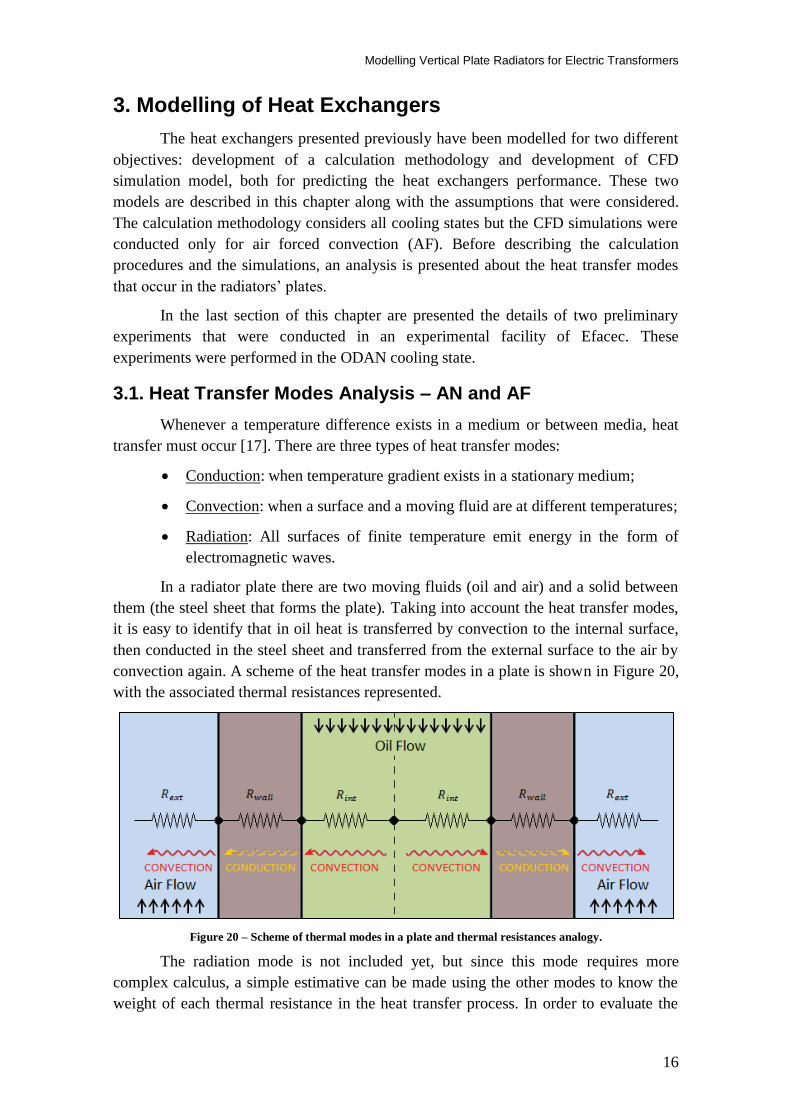
In a radiator plate there are two moving fluids (oil and air) and a solid between
them (the steel sheet that forms the plate). Taking into account the heat transfer modes,
it is easy to identify that in oil heat is transferred by convection to the internal surface,
then conducted in the steel sheet and transferred from the external surface to the air by
convection again. A scheme of the heat transfer modes in a plate is shown in Figure 20,
with the associated thermal resistances represented.
Figure 20 – Scheme of thermal modes in a plate and thermal resistances analogy.
The radiation mode is not included yet, but since this mode requires more
complex calculus, a simple estimative can be made using the other modes to know the
weight of each thermal resistance in the heat transfer process. In order to evaluate the

Modelling Vertical Plate Radiators for Electric Transformers
17
contribution of each mode in different cooling states, data from two real transformers
(Efacec transformers) was taken and can be seen in Table 3.
Table 3 - Data from two transformers, each one in two different cooling states
Transformer
Reference 546 A 767 A
Number of Radiators 12 18
Plates per Radiator 18 28
Plates Length [mm]
3 of 1800
15 of 2200
(per radiator)
All with 3200
Cooling State ONAN ONAF ODAN ODAF
Toil;in [ºC] 60.3 53 57 57
Tair;in [ºC] 23.5 26 19 19
Qoil;transformer[m3/h] 16.8 16.1 330 330
Qair;fan[m3/h] - 4400 - 10200
Fans per Radiator - 4 - 4
Fans Position - Side - Side
With this information and using correlations for oil and air, for natural and
forced convections, the thermal resistances were obtained. More information about this
calculation procedures are going to be presented in the next section.
In Table 4 is shown the percentual weight of the thermal resistances in the
different cooling states.
Table 4 – Thermal resistances of heat transfer modes in percentual weight, for four cooling states
Cooling State ONAN ONAF ODAN ODAF
%Rint 6.19% 21.01% 5.76% 22.44%
%Rwall 0.02% 0.08% 0.02% 0.08%
%Rext 93.79% 78.91% 94.22% 77.48%
As it can be seen from Table 4, the thermal resistance of heat conduction in the
plate walls has a very low weight in all cooling states (maximum of 0.08%). Therefore,
in order to simplify the calculation procedure, this resistance will be neglected and the
temperatures of the wall in the internal and external sides will be considered equal.
It is also important to notice that the thermal resistance in oil should not be
neglected since the results show that it contributes considerably in the heat transfer
process, especially if the fans are turned on (ONAF and ODAF states). This happens
because the increase in air velocity reduces its thermal resistance, while the oil
convection resistance remains the same increasing its relative weight.

Modelling Vertical Plate Radiators for Electric Transformers
18
3.2. Calculation Procedures – AN and AF
Reviewing some literature in heat transfer it was found that forced convection is
much more explored then natural convection and more Nusselt correlations for different
geometries are available in forced convection. It appears to be easier to model forced
convection, since the fluid flow is imposed and consequently the flow rate and/or the
fluid’s velocity typically are known. The same doesn’t happen in natural convection
because fluid’s motion results from buoyance forces caused by temperature gradients.
Knowing the value of fluids’ flow rate is very useful in heat transfer to calculate the
cooling capacities and fluids temperature at the end of the heat exchange.
In a transformer, buoyance forces that induce oil movement are generated by the
thermal gradients in the tank and in the radiators. Since the tank has greater volume than
the radiators, it is going to be assumed that the major contribute in oil motion is given
by the tank’s thermal gradients and so its convection will be treated in radiators as a
forced one. The values of oil flow rate in natural convection are taken from a simulation
tool for the tanks of transformers developed by Efacec.
As a consequence of this assumption, the oil flow rate was always an input data
in the following calculation procedures and forced convection correlations were used.
Thus OD and ON states have the same considerations in calculation methodology.
Concerning the air flow, forced and natural convection correlations are
employed when fans are turned on and off, respectively.
In the next subsection oil convection analysis is going to be presented first and
its considerations are valid for all cooling states. After that, air natural convection
procedures are stated, completing the methodology for ONAN and ODAN states, and
then air forced convection is considered, concluding ONAF and ODAF states. Finally in
the last subsection is presented the methodology used to include the radiation effect in
calculations.
3.2.1. Convective Heat Transfer Inside the Oil
In order to estimate the cooling capacity of the radiators, convective heat transfer
coefficients for oil and air have to be calculated. As previously stated, the oil flows
through a plate being divided in six identical channels. Using the design information in
[11] and Solidworks software, the internal and external perimeters of each channel were
estimated. The internal cross section of a channel and the external perimeter of the
entire plate were also calculated (these values are constant because the plate width is
always the same). These values are presented in Table 5.
Table 5 – Evaluation of some constant geometric parameters of a plate
Channel Internal Perimeter
Plate External Perimeter
Across;channel

Modelling Vertical Plate Radiators for Electric Transformers
19
With these values is possible to determine the heat transfer areas as well as the
channel hydraulic diameter using equations 3.1 to 3.3.
(3.1)
(3.2)
(3.3)
Where Aint, Aext, Dh;channel and L are the plate total internal area, the plate external
area, the channel hydraulic diameter and the plate length, respectively.
The oil flow regime was evaluated with the Reynolds number using the channel
hydraulic diameter (equation 3.4), since it is an internal flow.
( )
(3.4)
Where and are oil’s density and dynamic viscosity calculated at the oil
average temperature [17]. The Qoil;channel is the oil flow rate in a channel and it was
estimated considering that the oil flow is distributed equally by all plates and all
channels.
In all studied cases, was found to be much smaller than 2300, which
means the flow is laminar. According to [17], for laminar and fully developed flows the
Nusselt number can be obtained consulting the information in Figure 21.
Figure 21 – Nusselt numbers for fully developed laminar flow in tubes of different cross section [17].
The fully developed conditions were verified using equation 3.5 (where is
the hydrodynamic entry length [17]) and the ratio was estimated in approximately 7.
Taking this into account and considering a uniform wall temperature condition, the
Nusselt number is 5.60 (equation 3.6).

Modelling Vertical Plate Radiators for Electric Transformers
20
(3.5)
(3.6)
To determine the oil heat transfer coefficient in one channel, equation 3.7 was
used. With this value and knowing the channel heat transfer area (1/6 of the total
internal area), the channel thermal resistance can be obtained using 3.8.
(3.7)
(3.8)
Where , and are the channel internal heat transfer
coefficient, the oil thermal conductivity and the channel thermal resistance. Since there
are 6 channels in a plate, by the electric resistances analogy this corresponds to 6 equal
resistances in parallel and the total plate internal thermic resistance ( ) can be
obtained with equation 3.9.
(3.9)
Notice that all oil properties values are considered at the fluid’s average
temperature since this is an internal flow. These values are calculated with equations
that are function of temperature, being this equations extracted from company’s charts
(Annex A).
3.2.2. ONAN and ODAN states
The heat transfer process from oil to air can be seen as a series of two thermal
resistances system, with the oil temperature in one side and the air temperature in the
other. This is illustrated in Figure 22.
Figure 22 – Heat transfer as a series of thermal resistances.
The heat dissipation can be calculated with equation 3.10:
(3.10)
Where , , and are respectively the plate heat dissipation
(in watts), the oil average temperature, the air room temperature and the plate external

Modelling Vertical Plate Radiators for Electric Transformers
21
thermal resistance. Notice that the air temperature used is not the average between inlet
and outlet because in this case air convection is natural and so this values are not known
as well as the air flow rate.
To calculate is required the air convection coefficient. This coefficient may
be different at the inner and outer surfaces. In order to differentiate these convection
coefficients, the one for the inner surfaces was designated and the other . In
Figure 23 is a scheme of this nomenclature.
Figure 23 – Scheme of air convection coefficients nomenclature.
In this sequence there are two different external thermal resistances,
and , that were calculated using 3.11 and 3.12.
(3.11)
(3.12)
Notice that in equations 3.1 and 3.2, the internal and external areas were
calculated with the plate’s perimeter and so these areas as well as the thermal
resistances regard both sides of a plate. The total cooling capacity of a radiator was
obtained using equations (3.13) to (3.15).
(3.13)
(3.14)
( ) (3.15)
Where is the radiator’s cooling capacity and , and are
respectively the heat dissipated between two plates, the heat dissipated through the
surfaces at the ends and the number of plates present in the radiator.

Modelling Vertical Plate Radiators for Electric Transformers
22
The coefficient was calculated using a Nusselt correlation for isolated
vertical plates developed by Churchill and Chu [18] for laminar and turbulent natural
convection. This correlation is shown in equation 3.16 and in 3.17 is the Rayleigh
number that was used.
[
⁄
( ( ⁄ ) ⁄ ) ⁄ ]
(3.16)
( )
(3.17)
Where is the average surface temperature. Two hypotheses were made for
the air convection between plates (Figure 24):
The distance between plates is big enough so the thermal boundary layers
don’t overlap and each plate behaves as an isolated one.
The thermal boundary layers overlap and so the air flow is developing
between plates.
Figure 24 – Hypothesis for air convection between plates.
For the first hypothesis was calculated using the same correlation of ,
equation 3.16. For the second hypothesis equation 3.18 was used to calculate . The
Rayleigh number in this correlation is calculated using equation 3.19.
[ (
)]
(3.18)
( )
(3.19)
Equation 3.18 was proposed by Elenbaas in [19] for symmetrically heated
isothermal plates. This correlation was formulated considering two limits of parallel
plates’ arrangement: and (being S the distance between plates). When
considering the second limit, the correlation was adjusted to match the values of a free
vertical plate correlation. The correlation presented on equation 3.18 should be enough

Modelling Vertical Plate Radiators for Electric Transformers
23
to include both cases presented in Figure 24, the problem is that the free vertical plate
correlation used in [19] is valid in the laminar regime. Since the obtained values of
Rayleigh number in the current work indicate that the flow is turbulent, equation 3.16
was used to compare results. No correlation concerning natural convection in turbulent
flows between parallel plates was found.
In natural convection all properties were evaluated at the film temperature:
(3.20)
In order to use the described methodology, the values of oil outlet temperature
and surface temperature were initially arbitrated and then corrected, making iterations
with equations 3.21 and 3.22 taken from the energy balance.
( ) (3.21)
( ) (3.22)
The flowchart in Figure 25 summarizes the calculation procedure for ONAN and
ODAN systems.
Figure 25 - Calculation Procedure for ONAN and ODAN states.
3.2.3. ONAF and ODAF states
The general calculation procedure for ONAF and ODAF states is very similar to
the on for the previous cooling states, but the convective heat transfer coefficient is
calculated in a different way. This coefficient was also considered different in the inner
and outer plates, being named also and , respectively.
Two different considerations could be made: the air flow from the fans goes
through the gaps between plates and also goes to the outer surfaces or only between
plates (Figure 26).

Modelling Vertical Plate Radiators for Electric Transformers
24
Figure 26 - Two possible flow paths for the air from the fans.
It was considered that the forced air flow is driven only between plates and at the
outer surfaces only natural convection takes place. In the typical arrangements fans are
very close to radiators and so a little quantity or even none air flow should reach the
outer surfaces. Furthermore the air velocity in these surfaces would be difficult to
estimate.
It follows that will be determined using the already used correlation in
equation (3.16). In the gaps between plates a correlation for turbulent flow of a fluid
through a long narrow channel was used (equation 3.23). This correlation is proposed
by [2] to be applied in transformers’ radiators when cooled by fans. The Reynolds
number is presented in equation (3.24).
(3.23)
(3.24)
Where is the hydraulic diameter of the cross section between plates. This
diameter is different for air entering at radiator’s bottom and entering at its side,
equations 3.25 and 3.26. But since the plate width (W) and length (L) are much bigger
than the plate spacing (S), the hydraulic diameter can be approximated to two times the
plate spacing.
(3.25)
(3.26)
To calculate the air flow rate, the nominal flow rates of the fans cooling the
radiator are summed and divided by the number of existing gaps ( ). Then the air
velocity is calculated dividing this air flow by the cross area. Equations 3.27 and 3.28
were used for bottom and side ventilation, respectively.
∑ ( ) ( ) (3.27)
∑ ( ) ( ) (3.28)
For the air forced convection between plates, properties were evaluated at air
average temperature. This temperature was also used to calculate the cooling capacity,
instead of using the room temperature. This implies arbitrating air outlet temperature
and then correcting it with equation 3.29.

Modelling Vertical Plate Radiators for Electric Transformers
25
( ) (3.29)
3.2.4. Radiation
The radiation is a heat transfer mode that may assume an important role in the
radiators cooling capacity. In order to include this process between the plate surface and
the air a new circuit of thermal resistances must be considered, as shown in Figure 27.
Figure 27 – Thermal resistances circuit considering radiation.
Having one resistance in series with other two in parallel, the equivalent is
calculated using (3.30).
(3.30)
Where and are thermal resistances of radiation and air convection,
respectively. The air convection resistance was calculated in the same way as stated
previously.
A large percentage of the radiation emitted by the inner plates’ surfaces will be
absorbed by the opposite ones. The view factor concept was used to account the
radiation that doesn’t hit the other plates.
According to [17], the view factor for two aligned parallel rectangles can be
estimated using equation 3.31.
[ [(
( ) ( )
)
] ( )
(
( )
)
( )
(
( )
) ] (3.31)
Where F is the view factor and represents the fraction of radiation that leaves
one surface and reaches the other. The parameters x and y are calculated with 3.32 and
3.33.
(3.32)

Modelling Vertical Plate Radiators for Electric Transformers
26
(3.33)
To calculate the radiation dissipated by the plates and corresponding thermal
resistances, equations 3.34 to 3.37 were used.
( ) (
) (3.34)
(
) (3.35)
(3.36)
(3.37)
Where is the surface emissivity and is the Stefan–Boltzmann constant
( ).
3.3. CFD Simulations Methodology – AF
In order to evaluate the radiator behaviour in ONAF and ODAF cooling states,
CFD simulations were performed in Ansys Fluent v.15. The objectives of the conducted
simulations were:
Evaluate the entry region for different plate lengths and its impact on the
cooling capacity;
Estimate the radiators cooling capacity and compare it with the literature
correlation prediction;
Compare the surface constant temperature condition with a linear
temperature profile;
Compare cooling capacities between the two fans positions: side and bottom.
The air convection was the focus of the simulation because it represents the
major heat transfer resistance, its behaviour is harder to predict with correlations and the
air flow is difficult to measure in experiments. In this sequence the oil flow was not
modelled being the walls’ temperature an input condition.
The modelled geometry consists in a rectangular prism that represents the air
gap between two radiator plates. This geometry does not reflect the real wavy shape of
the plates, but modelling flat plates allows the construction of a mesh with orthogonal
and fewer elements, reducing the convergence time and ensuring accuracy.
Figure 28 shows a model for plates with 2200mm length and bottom ventilation.

Modelling Vertical Plate Radiators for Electric Transformers
27
Figure 28 – Model to simulate bottom ventilation between two plates – adapted from Ansys CFD-Post.
The air walls, as named in Figure 28, are virtual walls defined with adiabatic and
no slip boundary conditions. These walls were used to close the CFD model and doesn´t
exist in reality. They were created to simplify the model and since W/S >10 this
simplification shouldn’t have a great influence on the velocity profiles. However,
considering other type of boundaries may allow the evaluation of the air flow that enters
or leaves the gaps from the sides.
For the side ventilation cases, the air walls change their places with the inlet at
outlet surfaces. For all cases the model was divided in ten volumes in the air flow
direction in order to extract local values. The boundary conditions for the different
surfaces can be seen in Table 6.
Table 6 – Boundary conditions in CFD simulations
Surface Type Boundary Conditions
Inlet -Velocity Inlet
-Constant Temperature
Outlet -Pressure Outlet
Hot Wall
-Wall
-No Slip
-Temperature Linear Profile (or constant temperature)
Air Wall
-Wall
-No slip
-Adiabatic
Before performing the simulations, the Reynolds number was estimated using
different values from fans catalogues and the obtained results were all superior to 104.
This indicates that the air flow is in the turbulence regime and so the Standard k-ε

Modelling Vertical Plate Radiators for Electric Transformers
28
model with enhanced wall treatment was set. Energy equation was turned on, all
residuals were set to 10-6
and second order solutions were set to all equations.
A mesh study was conducted in order to find an optimal grid refinement. Special
attention was taken to the size of the elements next to the hot walls so that . This
condition is required to obtain accurate results from the enhanced wall treatment
function.
The mesh was evaluated using a geometry with 800mm length (y direction),
520mm width (x direction) and 45mm in the other direction (plate spacing – z direction).
The element size was established as 10% of the smaller edge, i.e. 4.5 mm, and then
refinement was made in z direction. This refinement was made decreasing the element
size and/or increasing the bias factor (ratio between the bigger and the smaller elements).
Table 7 shows the elements size and bias factors tested in the z direction, along with the
evaluation parameters used.
Table 7 – Mesh study results – refinement in z direction
Average
Element
Size [mm]
Bias
Factor y+
Heat
Flux
[W]
Inlet Static
Pressure
[Pa]
Maximum
Aspect
Ratio
Total
Number of
Elements
Mesh 1 4.5 1 36.8 334.5 3.63 1.74 208800
Mesh 2 2.25 1 18.0 326.2 3.74 2.97 417600
Mesh 3 2.25 10 4.46 340.8 4.14 11.5 417600
Mesh 4 2.25 20 2.58 323.6 3.93 19.1 417600
Mesh 5 1.4 30 1.26 316.5 3.85 38.6 689040
Mesh 6 1.4 35 1.12 316.3 3.85 43.3 689040
Mesh 7 1.3 40 0.95 316.2 3.84 50.8 730800
Also velocity profiles were analysed to ensure their independence from the grid.
These profiles were taken in middle lines in the geometry, indicated in Figure 29, and
the results for different meshes are shown in from Figure 30 to Figure 32.
Figure 29 – Middle lines where velocity profiles were analysed.

Modelling Vertical Plate Radiators for Electric Transformers
29
Figure 30 – Velocity profile in the middle line along Y coordinate.
Figure 31 - Velocity profile in the middle line along Z coordinate.
Figure 32 - Velocity profile in the middle line along X coordinate.
Analysing the above results and Table 7, it can be seen that the heat flux, the
inlet static pressure and the velocity profile along Y coordinate are stabilized at mesh 5.
The other two velocity profiles are similar to all meshes. Regarding y+ condition, it is
only verified at meshes 6 and 7. This grid refinement carries an increase in the number
and the maximum aspect ratio of elements, but they remain structured hexahedral
elements. In order to ensure accuracy in the results, mesh 7 was selected to conduct the
CFD simulations. This mesh can be seen in Figure 33.
4.0
4.1
4.2
4.3
4.4
4.5
4.6
4.7
0 200 400 600 800
Ve
loci
ty [
m/s
]
Y Coordinate [mm]
Line Along Y
Mesh 3
Mesh 4
Mesh 5
Mesh 6
Mesh 7
0.0
0.5
1.0
1.5
2.0
2.5
3.0
3.5
4.0
4.5
5.0
0 5 10 15 20 25 30 35 40 45
Ve
loci
ty [
m/s
]
Z Coordinate [mm]
Line Along Z
Mesh 3
Mesh 4
Mesh 5
Mesh 6
Mesh 7
0.0
0.5
1.0
1.5
2.0
2.5
3.0
3.5
4.0
4.5
5.0
0 50 100 150 200 250 300 350 400 450 500
Ve
loci
ty [
m/s
]
X Coordinate
Line Along X
Mesh 3
Mesh 4
Mesh 5
Mesh 6
Mesh 7

Modelling Vertical Plate Radiators for Electric Transformers
30
Figure 33 - Mesh 7 corner view and zoom at the side.
A base case was established with the conditions indicated in the second column
of Table 8. The parameters were changed (values in Table 8) creating different
combinations and a total of 56 simulations were performed with and average elapsed
time of 32 minutes per simulation.
Table 8 – Parameters values for different simulations
Base Case Value Other Values
Hot Walls Top
Temperature [ºC] 50.9
43.9
63.8
75.8
Hot Walls Temperature
Drop [ºC] 14.1
0
7.1
21.2
Plate Length [mm] 2200
800
1000
1500
3300
Air Inlet Temperature [ºC] 25.8 0
40
Air Inlet Velocity [m/s] 4.10 (Values in Annex B)
Plates in Series* [-] 1 2, 4 and 6
*This parameter is only applicable to side ventilation.
In a transformer, radiators are typically disposed in groups. For side ventilation,
one group of fans is responsible for cooling one group of radiators. In these cases air
flow will travel a distance equal to the plate width times the number of radiators in the
group. Geometries with different widths were created to simulate these situations,
representing two, four and six plates in series (last parameter in Table 8).
Modelling Vertical Plate Radiators for Electric Transformers
31
3.4. Experimental Details – AN
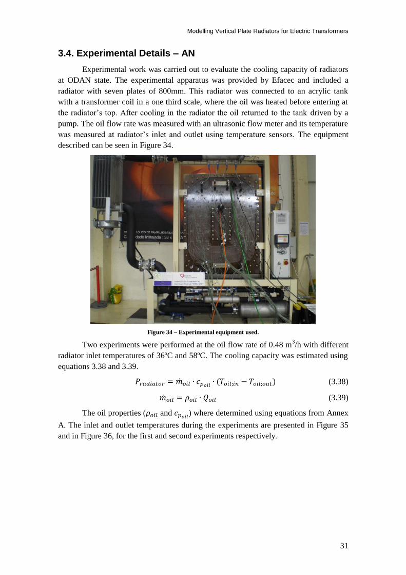
Experimental work was carried out to evaluate the cooling capacity of radiators
at ODAN state. The experimental apparatus was provided by Efacec and included a
radiator with seven plates of 800mm. This radiator was connected to an acrylic tank
with a transformer coil in a one third scale, where the oil was heated before entering at
the radiator’s top. After cooling in the radiator the oil returned to the tank driven by a
pump. The oil flow rate was measured with an ultrasonic flow meter and its temperature
was measured at radiator’s inlet and outlet using temperature sensors. The equipment
described can be seen in Figure 34.
Figure 34 – Experimental equipment used.
Two experiments were performed at the oil flow rate of 0.48 m3/h with different
radiator inlet temperatures of 36ºC and 58ºC. The cooling capacity was estimated using
equations 3.38 and 3.39.
( ) (3.38)
(3.39)
The oil properties ( and ) where determined using equations from Annex
A. The inlet and outlet temperatures during the experiments are presented in Figure 35
and in Figure 36, for the first and second experiments respectively.

Modelling Vertical Plate Radiators for Electric Transformers
32
Figure 35 – Inlet and outlet temperature during experiment 1.
Figure 36 - Inlet and outlet temperature during experiment 2.
For the first experiment 227 values of both temperatures were recorded by an
automaton and 18 values of oil flow rate were registered manually. Likewise, for the
second experiment 74 values for temperatures were registered and 11 for the oil flow
rate.
An uncertainty analysis was conducted for the two experiments. The registered
values were processed statistically to estimate the random uncertainty and information
from the equipment’s catalogues was used to evaluate systematic uncertainty. The total
uncertainty of each variable ( , and ) was obtained with equation 3.40.
√ (3.40)
Where , and are the total, random and systematic uncertainties,
respectively. Using the software EES (Engineering Equation Solver), the uncertainty
propagation was calculated and consequently the total uncertainty for the cooling
capacity was obtained with a confidence interval of 95%.
The procedure of uncertainty analysis is described in Annex C.
30
31
32
33
34
35
36
37
38
39
40
0 5 10 15 20 25 30 35 40
Tem
pe
ratu
re [
ºC]
Time [min]
Experiment 1
Inlet Temperature
Outlet Temperature
40
42
44
46
48
50
52
54
56
58
60
0 2 4 6 8 10 12
Tem
per
atu
re [
ºC]
Time [min]
Experiment 2
Inlet Temperature
Outlet Temperature

Modelling Vertical Plate Radiators for Electric Transformers
33
4. Results and Discussion
In this chapter the results are presented in two sections: Air Forced Convection
and Air Natural Convection. The results from calculation methodologies are compared
with other sources (CFD, experiments and transformers’ operational tests).
4.1. Air Forced Convection
The CFD simulations are the central focus of this section. In the first part, the
cooling capacities for flat plates in different conditions are presented, obtained directly
from CFD simulations. These results are compared with the calculated results using the
literature correlations presented previously. Then new correlations are formulated with
the CFD data, followed by a comparison between side and bottom ventilations. In the
last part, one of the new correlations is introduced in the calculation methodology and it
is applied in a real transformer case. In this case, the results using literature and using
the new correlation are compared with operational tests performed by the company.
4.1.1. CFD Simulation Results
The calculation procedure for air forced convection, previously presented on
subsection 3.2.3., was applied to flat plate geometry in order to allow the direct
comparison with CFD simulation results.
The cooling capacities are evaluated varying parameters one or two at the time,
whereas the other parameters are kept constant at the base case values. These values are
presented in Table 9.
Table 9 – Base case parameters values
Base Case Values
Hot Walls Top
Temperature
Hot Walls
Temperature Drop
Plate
Length
Air Inlet
Temperature
Air Inlet
Velocity
50.9 ºC 14.1 ºC 2200 mm 25.8 ºC 4.1 m/s
Figure 37 shows, for bottom ventilation, the cooling capacity variation with the
plates’ length. The respective data is showed in Table 10.

Modelling Vertical Plate Radiators for Electric Transformers
34
Figure 37 – Variation of cooling capacity with plate length; bottom ventilation.
Table 10 – Cooling capacities for different plate lengths and deviations of calculus from CFD results
Cooling Capacity
[W]
L[mm]
800 1000 1500 2200 3300
CFD Simulation 327.7 392.8 540.7 729.2 992.0
Calculation 265.0 326.2 469.6 652.2 903.5
Deviation [%] 19.1% 17.0% 13.2% 10.6% 8.9%
It can be seen in the results that the cooling capacities predicted from the
calculation procedure is always below the values provided by CFD simulation. The
percentage deviation decreases with the plate length, indicating that the air flow isn’t
fully developed in all cases and entrance effects should be taken into account since the
heat transfer is enhanced in the entry region. The evolution of both curves presented in
Figure 37 also shows that the variation is not linear, which indicates that the heat
transfer is not proportional to the plates’ area. This can be justified also with the entry
region effect: for longer plates a greater portion of the flow is fully developed having a
lower average heat transfer rate. Figure 38 presents the temperature distribution, for
different plates’ length, in a vertical section at the middle of the plates’ width.
0
100
200
300
400
500
600
700
800
900
1000
800 1300 1800 2300 2800 3300
Co
oli
ng
Cap
acit
y [W
]
L [mm]
Cooling Capacity vs. Plate Lenght
CFD Simulation
Calculation

Modelling Vertical Plate Radiators for Electric Transformers
35
Figure 38 – CFD temperature distribution between plates in a vertical section at the middle of the plates’
width.
The cooling capacities for different top wall temperatures are plotted in Figure
39, and the respective data is shown in Table 11. The impact of varying the wall
temperature drop is presented for two plate lengths, 2200 and 3300mm, on left and right
sides of Figure 40, respectively. The numerical values can be seen in Table 12 and
Table 13.
Figure 39 - Variation of cooling capacity with top wall temperature; bottom ventilation.
0
200
400
600
800
1000
1200
1400
1600
1800
2000
50 55 60 65 70 75
Co
olin
g C
apac
ity
[W]
Top Wall Temperature [ºC]
Cooling Capacity vs. Top Wall Temperature
CFD Simulation
Calculation

Modelling Vertical Plate Radiators for Electric Transformers
36
Table 11 - Cooling capacities for different top wall temperatures
and deviation of calculus from CFD results
Cooling
Capacity [W]
Top Wall Temperature [ºC]
50.9 63.8 75.8
CFD
Simulation 729.2 1243.8 1722.7
Calculation 652.2 1113.4 1538.2
Deviation [%] 10.6% 10.5% 10.7%
Looking at Table 11, the percentage deviation remains practically the same
revealing that the calculation procedure follows the simulations’ pattern for different top
wall temperatures.
Figure 40 - Variation of cooling capacity with wall temperature drop; bottom ventilation.
Table 12 - Cooling capacities for different wall
temperature drops, with L=2200mm.
Cooling Capacity [W]
(L=2200mm)
ΔT on wall [ºC]
7.1 14.1
CFD Simulation 864.5 729.2
Calculation 778.4 652.2
Deviation [%] 10.0% 10.6%
Table 13 - Cooling capacities for different wall
temperature drops, with L=3300mm.
Cooling Capacity [W]
(L=3300mm)
ΔT on wall [ºC]
14.1 21.2
CFD Simulation 992.0 813.8
Calculation 903.5 728.7
Deviation [%] 8.9% 10.5%
The above results show that for greater temperature drops the cooling capacity is
lower. Since top temperature is maintained constant, greater temperature drops imply
lower bottom wall temperatures and consequently a lower average temperature. This
explains why the cooling capacity decreases. On the other hand, having a lower average
wall temperature shouldn’t influence much the deviation between calculations and CFD
600
650
700
750
800
850
900
950
1000
6 8 10 12 14
Co
oli
ng
Cap
acit
y [W
]
Wall Temperature Drop [ºC]
Cooling Capacity vs. ΔT (L=2200mm)
CFD Simulation
Calculation
600
650
700
750
800
850
900
950
1000
14 16 18 20 22
Co
olin
g C
apac
ity
[W]
Wall Temperature Drop [ºC]
Cooling Capacity vs. ΔT (L=3300mm)
CFD Simulation
Calculation
Modelling Vertical Plate Radiators for Electric Transformers
37
results since this parameter has been altered also in a previous case (the one from Table
11) and it didn’t influence the deviations. However, as the temperature drop increases
the case gets more different from the constant surface temperature condition, which is
an assumption in the literature correlation. This explains the deviation increase.
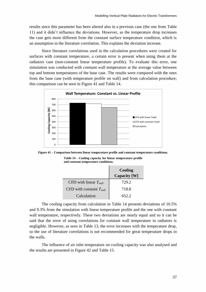
Since literature correlations used in the calculation procedures were created for
surfaces with constant temperature, a certain error is present when using them at the
radiators case (non-constant linear temperature profile). To evaluate this error, one
simulation was conducted with constant wall temperature at the average value between
top and bottom temperatures of the base case. The results were compared with the ones
from the base case (with temperature profile on wall) and from calculation procedure;
this comparison can be seen in Figure 41 and Table 14.
Figure 41 – Comparison between linear temperature profile and constant temperature conditions.
Table 14 – Cooling capacity for linear temperature profile
and constant temperature conditions.
Cooling
Capacity [W]
CFD with linear Twall 729.2
CFD with constant Twall 718.8
Calculation 652.2
The cooling capacity from calculation in Table 14 presents deviations of 10.5%
and 9.3% from the simulation with linear temperature profile and the one with constant
wall temperature, respectively. These two deviations are nearly equal and so it can be
said that the error of using correlations for constant wall temperature in radiators is
negligible. However, as seen in Table 13, the error increases with the temperature drop,
so the use of literature correlations is not recommended for great temperature drops in
the walls.
The influence of air inlet temperature on cooling capacity was also analysed and
the results are presented in Figure 42 and Table 15.
0
100
200
300
400
500
600
700
800
Co
olin
g C
apac
ity
[W]
Wall Temperature: Constant vs. Linear Profile
CFD with linear Twall
CFD with constant Twall
Calculation

Modelling Vertical Plate Radiators for Electric Transformers
38
Cooling Capacity vs. Air Inlet Temperature
Figure 42 – Air inlet temperature influence on cooling capacity.
Table 15 – Cooling Capacities for different air inlet and top wall temperatures
Twall;top 50.9 ºC 63.8 ºC
Tair;in 0 ºC 25.8 ºC 25.8 ºC 40 ºC
Cooling
Capacity
[W]
CFD
Simulation 1849.6 729.2 1243.8 660.1
Calculation 1662.1 652.2 1113.4 588.3
Deviation [%] 10.1% 10.6% 10.5% 10.9%
Evaluation of cooling capacity for air inlet temperature at 40ºC was performed
with 63.8ºC in the top wall because the base case has a bottom temperature of 36.8ºC,
which is inferior to 40ºC and it would lead to an unrealistic simulation (since the walls
temperatures cannot fall behind the air inlet temperature). To better analyse the impact
of changing air inlet temperature, the information was organized also in terms of the
difference between average wall temperature and air inlet temperature (Twall;ave - Tair;in).
This new analysis is presented in Figure 43.
Figure 43 – Cooling capacity variation with the temperature difference between wall and inlet air.
Looking at the results it is clear that the wall and air inlet temperatures have both
great influence on cooling capacity but their effect should be analysed together. For
0
200
400
600
800
1000
1200
1400
1600
1800
2000
0 5 10 15 20 25
Co
oli
ng
Cap
acit
y [W
]
Tair;in [ºC]
Twall;top= 50.9ºC
CFD Simulation
Calculation
0
200
400
600
800
1000
1200
1400
1600
1800
2000
25 30 35 40
Co
olin
g C
apac
ity
[W]
Tair;in [ºC]
Twall;top= 63.8ºC
CFD Simulation
Calculation
0
200
400
600
800
1000
1200
1400
1600
1800
2000
15 20 25 30 35 40 45
Co
olin
g C
apac
ity
[W]
Twall;ave - Tair;in [ºC]
Cooling Capacity vs. (Twall;ave-Tair;in)
CFD Simulation
Calculation

Modelling Vertical Plate Radiators for Electric Transformers
39
example supposing a case with wall top at 63.8ºC and air at 40ºC, changing these values
to 50.9ºC and 25.8ºC, respectively, only increases cooling capacity by 10%. This
happens because although air and wall temperatures have changed a lot, the temperature
difference increased only 1.3ºC. The calculation procedure follows the simulation curve
along these temperature variations since the deviations in Table 15 are very similar.
For analysing air inlet velocity, 14 levels of velocities were simulated for
different geometries. In Table 16 is the nomenclature attributed to different geometries
in order to facilitate the comparison.
Table 16 – Nomenclature attributed to different geometries
Name Description
2200 B L=2200mm; Bottom Ventilation
2200 S1 L=2200mm; Side Ventilation; 1 pair of plates (W=520mm)
800 B L=800mm; Bottom Ventilation
800 S1 L=800mm; Side Ventilation; 1 pair of plates (W=520mm)
800 S2 L=800mm; Side Ventilation; 2 pairs of plates (W=1040mm)
800 S4 L=800mm; Side Ventilation; 4 pairs of plates (W=2080mm)
800 S6 L=800mm; Side Ventilation; 6 pairs of plates (W=3120mm)
Air Inlet Velocity Influence on Deviations
Figure 44- Deviations on cooling capacities between calculation procedures and CFD simulations, for
different air inlet velocities and different geometries.
Figure 44 shows the air inlet velocity influence on deviation between calculation
and simulation results, for different geometries and for side and bottom ventilation.
The results show that for all models the deviation decreases with air inlet
velocity. Since the velocity profile is uniform at the entrance, higher inlet velocities
imply higher air volumetric flows (and mass flows also because the inlet temperature is
the same). The air temperature increase along the flow path is bigger for lower mass
flows and so it can be said that for low inlet velocities greater temperature increases
take place. Figure 45 shows this effect on 2200 B cases, representing for different
velocities the temperature evolution in a central axis along the flow direction.
0%
10%
20%
30%
40%
50%
60%
0 1 2 3 4 5
De
via
tio
n
Air Inlet Velocity [m/s]
2200 B
2200 S1
0%
10%
20%
30%
40%
50%
60%
0 1 2 3 4 5
De
via
tio
n
Air Inlet Velocity [m/s]
800 B
800 S1
800 S2
800 S4
800 S6

Modelling Vertical Plate Radiators for Electric Transformers
40
Figure 45 – Temperature evolution along flow direction for different inlet velocities.
If for smaller velocities the air temperature increases more, the density also
decreases more and the velocity profile will suffer more changes. This phenomenon
may be the cause for greater deviations at smaller velocities, since the correlations may
not respond to these changes.
Is important to notice that the higher deviations occur in the cases with velocities
below 2 m/s, where the Reynolds number is always above the turbulence lower limit.
Since calculation procedures were performed considering turbulent correlations and
simulations were conducted with a turbulence model, both methodologies may be
inaccurate out of the turbulence region.
Still analysing Figure 44, the different deviations between models can be
explained by the entry region effect. For example, the air flow travels a shorter distance
in 800 S1 cases (travelled distance of 520 mm) and higher deviations take place since
the entry length is a higher percentage of the total travelled distance. The lower
deviation occurs in the 800 S6 case because it has the greater travelling distance (6
plates in series give a total distance of 3120mm).
4.1.2. Formulation of New Correlations
In the previous subsection it was showed by the results from simulations that the
entry region has a great impact in the heat transfer between the walls and the air.
Analysing the deviations between the calculation procedure and the simulation, it was
concluded that the literature correlations used don’t take into account the entrance
effects. Taking this into account new correlations were developed to enhance the
calculation procedure accuracy.
To develop these new correlations, Nusselt and Reynolds numbers were
calculated using the data from CFD. From the 56 conducted simulations, only one was
excluded from this analysis because it didn’t correspond to a realistic situation: the one
with constant wall temperature condition. Two different correlations were developed:
one for bottom and another for side ventilation.
25
26
27
28
29
30
31
32
33
0 500 1000 1500 2000
Tem
pe
ratu
re [
ºC]
y [mm]
Temperature Evolution in Central Axis
In. Vel. - 1.5m/s
In. Vel. - 2.4m/s
In. Vel. - 3.6m/s
In. Vel. - 4.5m/s

Modelling Vertical Plate Radiators for Electric Transformers
41
According to [17], for turbulent internal flows a correlation of the form
presented in equation 4.1 can be used to calculate the average Nusselt number
considering the entry region.
[
( ⁄ ) ] (4.1)
Where , and are respectively the average Nusselt, the Nusselt in
the fully developed region and the distance in the flow direction. and are
parameters that depend on certain flow conditions, such us the nature of the inlet.
The first step was the determination of . For bottom ventilation the cases
with the longer plates (3300mm) should be used to calculate since this is the
situation were the flow is most developed. However, cases with 2200 and 3300 mm
plates were used as references to the fully developed flows because only 3 simulations
were conducted with the longer plates and performing more simulations with this
geometry would take more convergence time. Notice that in Table 10 the deviations for
the 2200 and 3300mm plates are not so different (10.6% and 8.9%) which means that
the assumption should cause small errors.
Figure 46 shows the Nusselt number depending on the Reynolds Number for
bottom ventilation simulations. It is also presented in the figure the trend line that better
fitted the values used for the fully developed condition.
Figure 46 – Nusselt depending on Reynolds, for bottom ventilation simulations.
0
10
20
30
40
50
60
70
80
90
100
0 5000 10000 15000 20000 25000 30000
Nu
Re
Nu vs. Re - Bottom Ventilation
CFD Simulations Undeveloped Flows
CFD Simulations Developed Flows
Laminar Reynolds
Turbulent Reynolds
Power Trend Line for Fully DevelopedNusselt

Modelling Vertical Plate Radiators for Electric Transformers
42
Table 17 – Comparison between regressions
for the for bottom ventilation
Regression Type R2
Exponential 0.9836
Linear 0.9975
Logarithmic 0.9845
Polynomial (order 2) 0.9978
Power 0.9987
Table 17 shows the coefficient of determination (R2) for different types of
regressions in order to know which fits better. The power function has been selected
since it presents the higher R2 and the correlation of is presented in equation 4.2.
(4.2)
The same procedure was performed for side ventilation and for the were
used the cases with 4 and 6 plates in series. These are the cases in which the air flow
travels a greater distance, for 4 plates is 2080mm and for 6 plates is 3120mm.
When using all simulations results for side ventilation, the power regression
didn’t fit well to the results (as showed in Figure 47).
Figure 47 - Nusselt depending on Reynolds, for side ventilation simulations.
Looking at Figure 47, one can see that some points are in the laminar zone
(Re<2300) and others are very close of the laminar limit. The simulations were made
with a turbulence model so Nusselt values on this zone are probably overestimated – if
these values were inferior the power regression would fit better. In this sequence the
points in or near the laminar zone were eliminated and the results were analyzed again
(Figure 48). Notice that in real radiators fans will induce velocities that correspond to
the turbulent regime, so the laminar zone has not much interest to this analysis.
0
10
20
30
40
50
60
70
80
90
100
0 5000 10000 15000 20000 25000 30000
Nu
Re
Nu vs. Re - Side Ventilation
CFD Simulations Undeveloped Flows
CFD Simulations Developed Flows
Laminar Reynolds
Turbulent Reynolds
Power Trend Line for Fully DevelopedNusselt

Modelling Vertical Plate Radiators for Electric Transformers
43
Figure 48 - Nusselt depending on Reynolds, for side ventilation simulations.
Now the power function fits well to the fully developed Nusselt. The coefficients
of determination (R2) of power, linear and second order polynomial regressions are very
similar and practically equal the unit (Table 18). The power function was selected to
correlate since this is the form that is found in literature.
Table 18 - Comparison between regressions
for the for side ventilation
Regression Type R2
Exponential 0.9861
Linear 0.9992
Logarithmic 0.9898
Polynomial (order 2) 0.9999
Power 0.9998
The obtained correlation for side ventilation in the fully developed region is
presented in equation 4.3.
(4.3)
Both bottom and side ventilation cases were correlated with the power function
for the fully developed condition, so the average Nusselt correlations will have the form:
[
( ⁄ ) ] (4.4)
The parameters C and m were determined by the minimization of the sum of the
squared differences between simulation results and values estimated by equations 4.2
and 4.3. The results of these adjustments are shown in Figure 49 for bottom ventilation
and in Figure 50 for side ventilation.
0
10
20
30
40
50
60
70
80
90
100
0 5000 10000 15000 20000 25000 30000
Nu
Re
Nu vs. Re - Side Ventilation
CFD Simulations Undeveloped Flows
CFD Simulations Developed Flows
Laminar Reynolds
Turbulent Reynolds
Power Trend Line for Fully DevelopedNusselt

Modelling Vertical Plate Radiators for Electric Transformers
44
Figure 49 – Adjustment of average Nusselt correlation for bottom ventilation.
Figure 50 – Adjustment of average Nusselt correlation for side ventilation.
The final correlations have shown to adjust very well to the simulation data in
both ventilation types and so the procedure to create them is concluded with success.
The final correlations for bottom and side ventilations are presented in equations 4.5
and 4.6.
[
( ⁄ ) ] (4.5)
[
( ⁄ ) ] (4.6)
4.1.3. Bottom vs. Side Ventilation
This subsection presents a focus on the comparison between cooling the radiator
plates with fans on their bottom and fans on their side. Figure 51 shows a comparison
between the two cooling configurations (side and bottom) presenting cooling capacities
for different air inlet velocities.
0
10
20
30
40
50
60
70
80
90
100
0 5000 10000 15000 20000 25000 30000
Nu
Re
Nu vs. Re - Bottom Ventilation
Bottom Ventilation Simulations
Average Nusselt Correlation
Laminar Reynolds
Turbulent Reynolds
0
10
20
30
40
50
60
70
80
90
100
0 5000 10000 15000 20000 25000 30000
Nu
Re
Nu vs. Re - Side Ventilation
Side Ventilation Simulations
Average Nusselt Correlation
Laminar Reynolds
Turbulent Reynolds
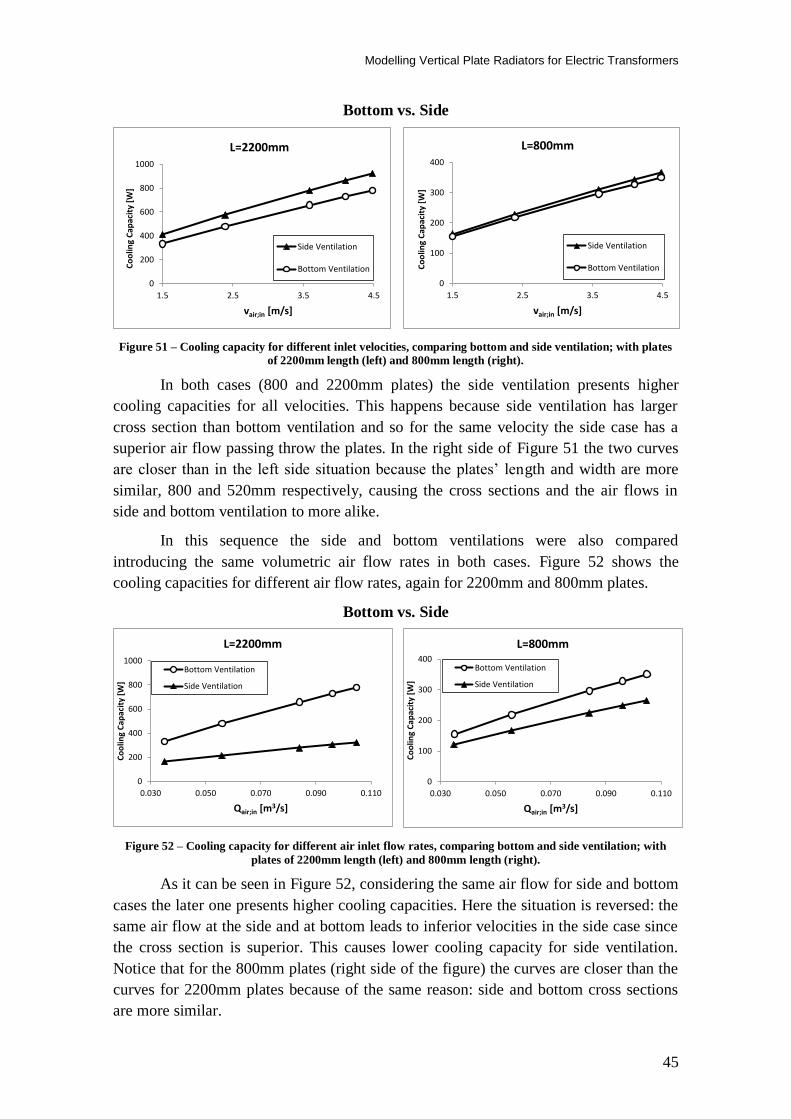
Modelling Vertical Plate Radiators for Electric Transformers
45
Bottom vs. Side
Figure 51 – Cooling capacity for different inlet velocities, comparing bottom and side ventilation; with plates
of 2200mm length (left) and 800mm length (right).
In both cases (800 and 2200mm plates) the side ventilation presents higher
cooling capacities for all velocities. This happens because side ventilation has larger
cross section than bottom ventilation and so for the same velocity the side case has a
superior air flow passing throw the plates. In the right side of Figure 51 the two curves
are closer than in the left side situation because the plates’ length and width are more
similar, 800 and 520mm respectively, causing the cross sections and the air flows in
side and bottom ventilation to more alike.
In this sequence the side and bottom ventilations were also compared
introducing the same volumetric air flow rates in both cases. Figure 52 shows the
cooling capacities for different air flow rates, again for 2200mm and 800mm plates.
Bottom vs. Side
Figure 52 – Cooling capacity for different air inlet flow rates, comparing bottom and side ventilation; with
plates of 2200mm length (left) and 800mm length (right).
As it can be seen in Figure 52, considering the same air flow for side and bottom
cases the later one presents higher cooling capacities. Here the situation is reversed: the
same air flow at the side and at bottom leads to inferior velocities in the side case since
the cross section is superior. This causes lower cooling capacity for side ventilation.
Notice that for the 800mm plates (right side of the figure) the curves are closer than the
curves for 2200mm plates because of the same reason: side and bottom cross sections
are more similar.
0
200
400
600
800
1000
1.5 2.5 3.5 4.5
Co
olin
g C
apac
ity
[W]
vair;in [m/s]
L=2200mm
Side Ventilation
Bottom Ventilation
0
100
200
300
400
1.5 2.5 3.5 4.5
Co
olin
g C
apac
ity
[W]
vair;in [m/s]
L=800mm
Side Ventilation
Bottom Ventilation
0
200
400
600
800
1000
0.030 0.050 0.070 0.090 0.110
Co
olin
g C
apac
ity
[W]
Qair;in [m3/s]
L=2200mm
Bottom Ventilation
Side Ventilation
0
100
200
300
400
0.030 0.050 0.070 0.090 0.110
Co
olin
g C
apac
ity
[W]
Qair;in [m3/s]
L=800mm
Bottom Ventilation
Side Ventilation

Modelling Vertical Plate Radiators for Electric Transformers
46
In the two comparisons made (fixing velocities and flow rates) one pair of plates
was only considered, so it is still not known if placing pairs of plates in series makes the
side ventilation more effective than bottom ventilation. To evaluate these situations,
cooling capacities were estimated for multiple pairs of plates, with the same total air
flow for side and bottom ventilation. A scheme for 3 pairs of plates is presented in
Figure 53. The cooling capacity results are shown in Figure 54.
Figure 53 – Three pairs of plates cooled by side and bottom ventilation.
Figure 54 – Cooling capacity for different number of plate pairs; L=2200mm.
The values presented in Figure 54 were estimated with the calculation procedure
but using the correlations obtained from simulation results. The analysis was performed
for flat plates with 2200mm length, with the same temperature profile on the walls and
air inlet temperature.
0
1000
2000
3000
4000
5000
6000
1 2 3 4 5 6
Co
olin
g C
apac
ity
[W]
Number of Plate Pairs
Bottom vs. Side Ventilation - Multiple Pairs of Plates(L=2200mm)
Bottom Vent.
Side Vent.

Modelling Vertical Plate Radiators for Electric Transformers
47
The results show that bottom ventilation is more efficient than side ventilation
until 4 pairs of plates and from there forward the situation is inverted. For each pair of
plates that is added to the arrangement, different things occur for the two configurations:
For bottom ventilation the total air flow increases in the same proportion of
the total cross section. Consequently the flow velocity is always the same,
the average heat transfer coefficient remains unchanged and the cooling
capacity increases linearly;
For side ventilation the total air flow increases but the cross section doesn’t
change. Therefore the flow velocity and the average heat transfer coefficient
increase, enhancing the cooling capacity and the heat transfer efficiency.
This explains the pattern of the curves in Figure 54. In fact, the situation in
which side overcomes bottom ventilation is when its flow average velocity becomes
superior. Following this logic, it is expected that using smaller plates the two
configurations (side and bottom) equalize their average flow velocity with less pairs of
plates. This was confirmed repeating the calculation for plates with 800mm length (see
Figure 55).
Figure 55 – Cooling capacity for different number of plate pairs; L=800mm.
Generally speaking, choosing side or bottom ventilation depends on the number
of radiators in series and the length of their plates. Notice that in the studied cases it was
assumed that the same quantity of air flow can be induced at the radiators side and
bottom. In reality the induced air flow depends, among other things, on the number of
fans cooling the radiators. Therefore another important aspect to choose side or bottom
ventilation is the number of fans that can be coupled to radiators in each configuration.
4.1.4. Transformer 546A in ONAF
The calculation method was employed in a real transformer from Efacec
operating in ONAF (Oil Natural Air Forced) in order to evaluate the accuracy of this
methodology.
0
500
1000
1500
2000
2500
3000
3500
4000
4500
5000
1 2 3 4 5 6
Co
olin
g C
apac
ity
[W]
Number of Plate Pairs
Bottom vs. Side Ventilation - Multiple Pairs of Plates(L=800mm)
Bottom Vent.
Side Vent.

Modelling Vertical Plate Radiators for Electric Transformers
48
Transformer 546A is a power transformer and its cooling system consists in 12
radiators cooled by 16 fans. These components are arranged in 4 groups, having each
group 3 radiators and 4 fans attached to the side of the first radiator (see Figure 56).
Figure 56 – Scheme of a radiator group of transformer 546A.
Each radiator has 18 plates, 15 of them with 2200mm length and the other three
with 1800mm. The average cooling capacity of each radiator was estimated using
values from operation tests performed on the transformer by Efacec. The test data was
compared with calculation procedures with three different conditions:
Considering the literature correlation;
Considering the correlation obtained from simulation results for side
ventilation;
Considering the correlation obtained from simulations and adding the
radiation heat transfer mode.
To make this comparison, the same values of temperature and oil flow rate
reported in the test were considered in the calculation procedures. These parameters are
presented in Table 19.
Table 19 - Operating conditions of transformer 546A in ONAF
Oil Flow Rate per Radiator 1.3 m3/h
Inlet Oil Temperature 53 ºC
Room Temperature 26 ºC
The average cooling capacity per radiator is presented in Figure 57. The
numerical values and the deviations from the test data are shown in Table 20.

Modelling Vertical Plate Radiators for Electric Transformers
49
Figure 57 – Radiator’s cooling capacity comparison from four different sources.
Table 20 – Radiator’s Cooling Capacity and deviations from test data
Cooling
Capacity [kW] Deviation
From Test Data 11.1 -
Sim. Correlation + Radiation 10.7 3.9%
Sim. Correlation 10.4 6.3%
Literature Correlation 9.3 16.2%
As it can be seen from the above results, the estimates provided by calculation
procedures with the new correlation reveal low deviations from test results (3.9%
considering radiation and 6.3% considering only air convection). The radiation
approach seems adequate since it led to a result with an inferior deviation from the
operation test. The literature correlation shows a higher deviation and so its application
to vertical plate radiators is not recommended.
Notice that due to the nature of the performed test, the uncertainty of the cooling
capacity value cannot be calculated. Making experimental tests with uncertainty
analysis allow a better validation of the calculation procedure.
4.2. Air Natural Convection
The calculation procedure for air natural convection was evaluated by its
application in three case studies: the experiments previously reported in section 3.4., a
transformer from Efacec and the experiments conducted in [5] (already mentioned on
the State of the Art).
4.2.1. Experimental Results
As stated before, two experiments were conducted on a radiator with 7 plates of
800mm length. The average values for the oil flow rate, the oil temperature at radiator’s
inlet and outlet, the room temperature and the calculated cooling capacity are listed in
Table 21.
0
2
4
6
8
10
12
Pra
dia
tor
[kW
]
Transformer 546A in ONAF
Literature Correlation
Sim. Correlation
Sim. Correlation +Radiation
From Test Data

Modelling Vertical Plate Radiators for Electric Transformers
50
Table 21 – Experimental average values
Experiment 1 Experiment 2
Room Temperature [ºC] 15.5 15.6
Inlet Oil Temperature [ºC] 36.4 57.5
Outlet Oil Temperature [ºC] 32.1 47.7
Oil Flow Rate [m3/h] 0.48 0.47
Cooling Capacity [W] 955 2135
The total uncertainties with 95% confidence of the cooling capacity values are
presented in Table 22.
Table 22 – Cooling capacity uncertainty for the two experiments
Experiment 1 Experiment 2
Total
Uncertainty 183 W (19%) 244 W (11%)
The above results show a high uncertainty associated to the experimental cooling
capacity values (maximum of 19%). The experiments were performed at a very low oil
flow rate, in which the flow meter presents lower accuracy (5% of systematic error by
the manufacturer’s catalogue). To obtain a systematic error of 1%, the oil flow rate
should be equal or superior to 2.3 m3/h. The temperature values present lower
uncertainties (average of 1.3%) than the oil flow rate, but its contribution to the
uncertainty on the cooling capacity is higher in the first experiment (according to EES
software). So the total uncertainty on cooling capacity can be reduced operating at
higher flow rates and temperatures. More details about the uncertainty analysis are
presented on Annex C.
The experimental results were compared with calculation procedures making
four different considerations that are described in Table 23. The results provided by
these methods are presented in Table 24.
Table 23 – Nomenclature for calculation procedures according to different considerations
Name Description
Method 1
Using the isolated vertical plate correlation for the
air convection between plates. This correlation is
presented in equation 3.16 (section 3.2.)
Method 2
Using the parallel plate correlation for the air
convection between plates. This correlation is
presented in equation 3.18 (section 3.2.)
Method 1 Rad The same as Method 1 but including the radiation
heat transfer mode.
Method 2 Rad The same as Method 2 but including the radiation
heat transfer mode.

Modelling Vertical Plate Radiators for Electric Transformers
51
Table 24 – Cooling capacity from calculation methods
Cooling Capacity
[W] Experiment 1 Experiment 2
Method 1 479 1125
Method 2 434 1001
Method 1 Rad 604 1380
Method 2 Rad 562 1266
The cooling capacities obtained from experiments and from calculation
procedures are plotted in Figure 58. The calculation deviations from the experimental
values are presented in Table 25.
Figure 58 – Comparison between experimental and calculation cooling capacities values.
Table 25 – Deviation of calculated cooling capacities from the experimental results
Deviations Experiment 1 Experiment 2 Average
Method 1 Rad 37% 35% 36%
Method 2 Rad 41% 41% 41%
Method 1 50% 47% 49%
Method 2 55% 53% 54%
The calculation procedures show high deviations (from 35% to 55%) on the
cooling capacity prediction, which are out of the uncertainty range associated to the
experimental results. The values obtained from calculation methodology are all below
the ones provided by the experiments and it can be explained by three possible
hypotheses:
Since the plates are short the air boundary layers on the plates’ surfaces
remain well separated, like two vertical isolated plates but with a higher heat
transfer rate. According to [20], the heat transfer in a parallel plate
arrangement can be higher than in the isolated plate case, duo to induced
flow by the chimney effect;
0
500
1000
1500
2000
2500
35 40 45 50 55 60
Rad
iato
r C
oo
ling
Cap
acit
y [W
]
Toil;in [ºC]
Cooling Capacity vs Oil Inlet Temperature
Experiments
Method 1 Rad
Method 2 Rad
Method 1
Method 2

Modelling Vertical Plate Radiators for Electric Transformers
52
The literature correlations are unable to reflect the heat transfer process in
radiators, since the plates aren’t flat and the temperature is not constant
along the surfaces – two conditions imposed by the correlations;
The radiation approach is under estimated.
The first two hypotheses can both be solved creating new correlations to the
vertical plate radiators. For this proposition more experiments or simulations have to be
performed. The third hypothesis is improbable to be the major cause of deviations, since
the radiators plates present a symmetric disposition causing a surface to intercept a great
fraction of the radiation leaving the other surface in front.
Despite of the high deviations presented by the calculation, notice that
considering the radiation mode enabled a significant increase in the cooling capacity; it
increased on average 24% for Method 1 and 28% for Method 2.
4.2.2. Transformer 546A in ONAN
The four calculation methods previously described in Table 23 were applied in
one Efacec’s transformer case. The transformer is the model 546 A, already described in
subsection 4.1.4. but this time operating in the ONAN state (Oil Natural Air Natural).
The average cooling capacity of each radiator was estimated using values from
operation tests performed on the transformer by the company. To compare this test with
the calculation procedure the same values of temperature and oil flow rate were used
and are presented in Table 26.
Table 26 – Operating conditions of transformer 546A in ONAN
Oil Flow Rate per Radiator 1.4 m3/h
Inlet Oil Temperature 60.3 ºC
Room Temperature 23.5 ºC
The comparison between the test data and the results from calculation methods
is presented in Figure 59 and Table 27.
Figure 59 – Radiator’s cooling capacity results.
0
1
2
3
4
5
6
7
8
Pra
dia
tor
[kW
]
Transformer 546A in ONAN
Method 2
Method 2 Rad
Method 1
Method 1 Rad
Test

Modelling Vertical Plate Radiators for Electric Transformers
53
Table 27 – Cooling capacity for one radiator of transformer 546A in ONAN
Radiator’s Cooling
Capacity [kW]
Deviation from
Test
Test 7.7 -
Method 1 Rad 6.5 15%
Method 1 5.7 26%
Method 2 Rad 5.4 30%
Method 2 4.4 43%
The results show once again that the cooling capacity predicted by calculations
procedures is below the test results. Notice that the deviations are much lower than in
the case presented in the previous subsection. Since the radiators of transformer 546A
have plates of lengths 1800 and 2200mm, longer than the ones of the previous case
(800mm), it is expected that a greater portion of the air flow is developed. This way the
average heat transfer rate is lower for the 546A case and it explains why the calculation
results are closer from the test.
Looking at the values in Table 27, it can be seen that now Method 1 gives a
higher cooling capacity than Method 2 Rad, unlike in the radiator with 800mm length.
This is justified by the different responses that the two correlations have in the cooling
capacity by changing the length of the plates. In order to clearly see these responses, the
4 methods were compared in terms of cooling capacity variation with the plates’ length.
The comparison was performed considering a radiator with 18 equal plates and fixing
the other parameters at the values presented in Table 26. The results can be seen in
Figure 60.
Figure 60 – Cooling capacity calculated by the four methods for different plate lengths.
In Figure 60 can be seen that the curves present different slopes and the results
present larger differences for longer plates. It can be seen also that Method 1 starts to
exceed Method 2 Rad at 1400mm.
0.0
2.0
4.0
6.0
8.0
10.0
800 1100 1400 1700 2000 2300 2600 2900 3200 3500
Pra
dia
tor
[kW
]
L [mm]
Cooling Capacity vs Plates Length
Method 2
Method 2 Rad
Method 1
Method 1 Rad

Modelling Vertical Plate Radiators for Electric Transformers
54
4.2.3. Hyosung Experiments
As stated before in the State of the Art section, Min-gu Kim et al. [5] performed
experiments on vertical plate radiators, supported by the Hyosung Corporation. These
experiments were conducted in a group of 4 radiators, each with 40 plates of 3300mm.
Three experiments were conducted, one in ONAN and the other two in the ODAN state.
The experimental data reported are shown in Table 28.
Table 28 – Experimental data from [5]
Experiment 1 Experiment 2 Experiment 3
Cooling State ONAN ODAN ODAN
Oil Flow Rate per Radiator 0.001 m3/s 0.0033 m
3/s 0.0042 m
3/s
Inlet Oil Temperature 89.3 ºC 88.8 ºC 88.3 ºC
Room Temperature 34.3 ºC 33.8 ºC 33.3 ºC
The four calculation methods seen in the previous subsections were applied in
the conditions of Table 28 and the cooling capacity results were compared with the ones
from the experiments. This comparison is presented in Figure 61 and Table 29.
Figure 61 – Cooling capacity for different oil flow rates; comparison between the calculation procedures and
the experiments from [5].
20
22
24
26
28
30
32
34
36
38
40
42
0 0.001 0.002 0.003 0.004 0.005
Pra
dia
tor
[kW
]
Qoil;radiator [m3/s]
Cooling Capacity vs Oil Flow
Method 1 Rad
Method 1
Experimental Results
Method 2 Rad
Method 2

Modelling Vertical Plate Radiators for Electric Transformers
55
Table 29 – Experimental cooling capacities from [5] and calculation results.
Cooling Capacity [kW] Average
Deviation
from
Experiments
Experiment
1
Experiment
2
Experiment
3
Experimental
data from [5] 27.4 1.7 32.4 1.8 33.0 1.6 -
Method 1 Rad 33.3 39.0 39.6 21%
Method 1 29.6 34.2 34.7 6%
Method 2 Rad 25.8 29.0 29.3 9%
Method 2 21.4 23.6 23.8 26%
The results show that for this case study the predictions on cooling capacities
from Method 1are above the experimental results and the ones from Method 2 are below
the experiments. Looking only at this case, the results would suggest that the air flows
in these experiments are between the isolated vertical plates situation and the fully
developed state, since Method 1 uses a correlation for the first situation and Method 2
uses a correlation for the second. In fact this cannot be concluded, considering the other
two case studies (subsections 4.2.1. and 4.2.2.) in which all calculation methods are
below the experimental data. All the studied correlations for air natural convection that
were analysed are not accurate for predicting the radiators’ cooling capacity, especially
for cases with small plates.
It is important to notice that between the three case studies the length of the
plates is not the only parameter that is changed. The number of plates per radiator
increases (7, 18 and 40 plates per radiator) as well as the oil flow rates per plate. These
two parameters can also influence the different deviation from the calculations
methodology.

Modelling Vertical Plate Radiators for Electric Transformers
56
5. Conclusions and Future Work
The modelling of vertical plate radiators for predicting their cooling
performance was conducted successfully. Two calculation methodologies were
developed, one for air forced convection and other for air natural convection. The first
methodology applies to ONAF and ODAF cooling states and the second applies to
ONAN and ODAN states. Both procedures turn out to be good techniques to design and
optimize transformers' radiators, since the heat transfer correlations respond to the
operational parameters variation (temperature, oil flow rate, air flow rate, etc.). For air
forced convection cases, new correlations were developed using CFD simulation to
improve the calculation methodology and it presented great accuracy when applied to
the radiators of a real transformer (cooling capacity deviations from company tests of
3.9%). However, for the cases with air natural convection, the literature correlations
provide results with high deviations comparatively to experiments and company tests.
The CFD models developed, consisting on rectangular prisms to represent
individual air gaps between radiator’s plates, proved to be a good and simple approach
to evaluate air forced convection in radiators. Results show that the air flows between
radiators’ plates are not fully developed, causing a great impact in the heat transfer and
errors in the cooling capacity estimated with literature correlations. The literature
correlations applied in the smallest radiator plates present the highest deviations from
CFD simulations, since in this case the air flow has a greater portion in the entry region.
The created correlations adjust successfully to the simulations results and reflect the
heat transfer enhancement by the entry region effect.
The average temperature of the walls and the air temperature are two parameters
that should be analysed together. When these temperature values are changed, the
cooling capacity does not change much if the difference between them is maintained.
Cases with very low inlet velocities reveal high deviations between simulations and the
calculation methodology, revealing that the turbulence model in simulation and/or the
literature correlation aren’t able to describe the heat transfer in the laminar region. This
does not affect the analysis of air forced convection in radiators, since the air flow
induced by the fans is always in the turbulent region.
A comparison between ventilating radiators with fans at the side and at the
bottom was performed. On one hand, the results show that for the same air inlet
velocities the side ventilation presents greater cooling capacities than bottom ventilation.
On the other hand, introducing the same air flow rate the results are inverted. This
happens because of the different cross sections on the side and on the bottom
configurations, causing superior flow rates for side ventilation when fixing the
velocities and superior velocities for bottom ventilation when fixing the air flow rates.
Cooling multiple radiators in series with side ventilation was compared with
cooling the same amount of radiators with fans on the bottom. The results show that
until a certain number of radiators the bottom ventilation is the most effective option,
but for more radiators the side ventilations takes the lead. That number of radiators, in
which the transition occurs, depends on the length of the plates and the number of fans
that can be coupled in each configuration.

Modelling Vertical Plate Radiators for Electric Transformers
57
Regarding the air natural convection, four different calculation methodologies
were evaluated in three case studies. Comparing to the other methodologies, Method 1
and Method Rad 1 presented cooling capacity results closer to the experimental data.
However, since these methods use a correlation for isolated vertical plates and the
results are above the experiments in the last case study, it can be concluded that the
radiator plates don’t behave like isolated surfaces in all situations. Method 2 Rad and
Method 2 present high deviations for radiators with 800mm to 2200mm length (up to
55%) and lower ones for 3300mm (9% for Method 2 Rad and 26% for Method 2). Thus
the correlation used in these methods is not accurate on predicting the cooling
performance of vertical plate radiators. New correlations have to be developed,
performing experiments or simulations, in order to enhance the accuracy of the
calculation methodology for ONAN and ODAN cooling states.
Radiation reveals to be a mechanism of great importance in radiators heat
dissipation, especially when air convection is natural (results reveal an increase on
cooling capacity up to 29% by the addition of the radiation mode). Therefore radiation
should be considered in the calculation methodologies.
Regarding future work, several studies can be conducted to better understand the
radiators behaviour, namely:
Evaluation of the air flow induced by fans. Although the created correlations
for air forced convection provided accurate results, they depend on the air
velocity and this parameter is estimated using the fans nominal air flow and
the cross section between plates. This procedure may not be the most
adequate since it doesn’t reflect the distribution of the fans on the available
area at the radiator.
Study of the impact of the number of plates in the cooling performance. The
number of plates in a radiator influences the amount of oil flow passing
through each plate and consequently affects the cooling capacity. The impact
of the number of plates has to be accounted to improve the prediction of the
cooling performance.
Evaluation of the correlations developed for air forced convection. Although
the new correlations presented great accuracy for the studied transformer,
they should be evaluated in other experimental case studies to validate their
accuracy in different conditions.

Modelling Vertical Plate Radiators for Electric Transformers
58
6. References
[1] Efacec website. Page consulted on April 2014, http://www.efacec.pt
[2] R. M. Del Vecchio et al., Transformer Design Principles: With Applications to Core-Form
Power Transformers, 2001.
[3] R. Hosseini et al., Determination of OD cooling system parameters based on thermal
modeling of power transformer winding, Simulation Modelling Practice and Theory, 2008.
[4] European Commission website. Page consulted on May 2014, http://ec.europa.eu.
[5] M.-g. Kim et al., Prediction and evaluation of the cooling performance of radiators used in
oil-filled power transformer applications with non-direct and direct-oil-forced flow, Exp. Therm.
Fluid Sci., 2012.
[6] International Electrotechnical Commission, 2011. IEC 60076-2 Power Transformers – Part
2: Temperature rise for liquid-immersed transformers.
[7] Imad-U-Khan et al., Dissolved Gas Analysis of Alternative Fluids for Power Transformers,
2007.
[8] F. Delgado et al., Fluid-thermal analysis of the cooling capacity of a commercial natural
ester in a power transformer, 2013.
[9] Engineering Craft Industries website. Page consulted on April 2014,
http://www.engineeringcraft.in
[10] Eurocooler Document, Technical Catalogue, May 2009.
[11] Eurocooler Document, Radiateurs pour Transformateurs, Documentation générale,
October 1996.
[12] Efaflu Document, Cooling Fans and Pumps for Power Transformers, May 2009.
[13] Krenz & Company, Inc. website. Page consulted on April 2014, http://www.krenzvent.com
[14] H. Nabati, J. Mahmoudi, Numerical Modeling of a Plane Radiator Used in a Power
Transformer Cooling System, 2008.
[15] H. Nabati, J. Mahmoudi, Simulation of Power Transformer’ Cooling System in ONAN State,
2008.
[16] R. Fdhila et al., Thermal modeling of power transformer radiators using a porous
medium based CFD approach, 2011.
[17] F. P. Incropera et al., Fundamentals of Heat and Mass Transfer, 7th Edition, 2011.
[18] S.W. Churchill and H.S. Chu, Correlating Equations for Laminar and Turbulent Free
Convection from a Vertical Plate, 1975.
[19] W. Elenbaas, Heat Dissipation of Parallel Plates by Free Convection, 1942.
[20] W. M. Rohsenow et al., Handbook of Heat Transfer, 3rd
Edition, 1998.
[21] Hugh W. Coleman and W. Glenn Steele, Experimentation, Validation, and Uncertainty
Analysis for Engineers, 3rd
Edition, 2009.

Modelling Vertical Plate Radiators for Electric Transformers
59
Annex A: Oil and Air Properties
The reference of the mineral oil used in Efacec’s transformers is Nynas Taurus.
This oil has a volumetric thermal expansion coefficient of 0.00064 K-1
. The equations
for the other properties depending on temperature were taken from company graphs and
are showed from equation A.1 to A.4. In these equations the temperature is in ºC.
(A.1)
(A.2)
[ ( )] (A.3)
(
)
(A.4)
The air properties were taken using tabulated data from [17] that was plotted.
The equations were extracted with trend lines. The plots are in Figures A.1 to A.4 and
the equations are presented in A.5 to A.8. The volumetric thermal expansion coefficient
was calculated with A.9 considering the air an ideal gas. In these equations the
temperature is in kelvin.
Figure A.1 – Air density as a function of temperature.
Figure A.2 – Air specific heat at constant pressure as a function of temperature.
y = 357.45x-1.004
R² = 1
0.0
0.5
1.0
1.5
2.0
2.5
3.0
3.5
4.0
0 500 1000 1500 2000 2500 3000 3500
ρ[kg/m3]
T [K]
ρ (T)
y = -4E-07x3 + 0.0008x2 - 0.3493x + 1047.7R² = 0.9999
980
1000
1020
1040
1060
1080
1100
1120
1140
1160
0 200 400 600 800 1000 1200
cp[J.kg-1.K-1]
T [K]
cp (T)

Modelling Vertical Plate Radiators for Electric Transformers
60
Figure A.3 – Air dynamic viscosity as a function of temperature.
Figure A.4 – Air density as a function of temperature.
(A.5)
(A.6)
( ) (A.7)
(A.8)
(A.9)
y = 1E-07x3 - 0.0004x2 + 0.6923x + 9.957R² = 1
0
50
100
150
200
250
300
350
400
450
0 200 400 600 800 1000 1200
μ . 107
[Pa.s]
T [K]
μ(T)
y = 4E-14x4 - 9E-11x3 + 3E-08x2 + 8E-05x + 0.0017R² = 1
0
0.01
0.02
0.03
0.04
0.05
0.06
0.07
0.08
0 200 400 600 800 1000 1200
k[W.m-1.K-1]
T [K]
k(T)

Modelling Vertical Plate Radiators for Electric Transformers
61
Annex B: Parameters of CFD Simulations
The values used in CFD simulation for all parameters are listed in Table B.1.
Table B.1 – Values for the CFD simulation parameters
[ ] [ ] [ ] [ ]
[ ]
Plates in
Series
Base Case
( ) 50.9 14.1 2200 25.8 4.10 1
43.9 0 800 0 0.35 2
63.8 7.1 1000 40 0.56 4
75.8 21.2 1500 0.85 6
3300 0.97
1.06
1.50
1.55
2.33
2.39
2.67
2.91
3.59
4.48
A total of 56 simulations were performed by making different combinations of
the parameters’ values. The first and second simulations were conducted for the base
case values and for bottom and side ventilations. The other 54 combinations are listed in
Table B.2 and Table B.3, for bottom and side ventilations respectively. The
combinations are identified mentioning the variables that are different from the base
case, using the code presented in Table B.1.
Table B.2 – Combinations for bottom ventilation

Modelling Vertical Plate Radiators for Electric Transformers
62
Table B.3 – Combinations for side ventilation

Modelling Vertical Plate Radiators for Electric Transformers
63
Annex C: Experiments Uncertainty Analysis
According to [21], the random uncertainty with 95% confidence for sample
populations can be calculated with equation C.1.
(C.1)
Where , and are the random uncertainty, the t-distribution for a 95%
confidence interval and the sample standard deviation, respectively. For the performed
experiments three variables were measured: the oil inlet temperature, outlet temperature
and volumetric flow rate. Considering the number of measures (N) for each variable and
the degrees of freedom (N-1), the random uncertainties were estimated and are
presented in tables C.1 and C.2 for the experiments 1 and 2, respectively.
Table C.1 – Random uncertainty estimation for experiment 1
[ ] [ ] [ ]
Average 36.41 32.09 0.48
N 227 227 18
Deg. of Freedom 226 226 17
0.1190 0.1133 0.009884
1.971 1.971 2.110
0.23 0.22 0.02
Table C.2 – Random uncertainty estimation for experiment 2
[ ] [ ] [ ]
Average 57.48 47.73 0.4688
N 74 74 11
Deg. of Freedom 73 73 10
0.1221 0.1240 0.01233
1.993 1.993 2.228
0.24 0.25 0.03
The systematic uncertainty ( ) was assumed equal to the measurement
accuracy of the temperature sensors and the flow meter, taken from these apparatus
catalogues. The total uncertainties ( ) of the variables were calculated using equation
C.2 and are presented in tables C.3 and C.4 for the experiments 1 and 2, respectively.
√ (C.2)

Modelling Vertical Plate Radiators for Electric Transformers
64
Table C.3 – Uncertainties for experiment 1
[ ] [ ] [ ]
0.23 0.22 0.02
0.50 0.50 0.024
0.55 0.55 0.031
Table C.4 – Uncertainties for experiment 2
[ ] [ ] [ ]
0.24 0.25 0.03
0.50 0.50 0.024
0.55 0.56 0.038
The cooling capacity was calculated using the average values of the
temperatures and the oil flow rate. Using the software EES (Engineering Equation
Solver), the uncertainty propagation was made and consequently the total uncertainty
for the cooling capacity was obtained with a confidence interval of 95%. The final
results are shown in figures C.1 and C.2 for the experiments 1 and 2, respectively.
Figure C.1 – Final results for experiment 1.
Table C.2 – Final results for experiment 2.