Modelling usingStochastic DifferentialEquations

Henrik Madsen

LVI Conference ofLithuanian Mathematicians Society

hmad@dtu.dk,www.henrikmadsen.org

Henrik Madsen 1

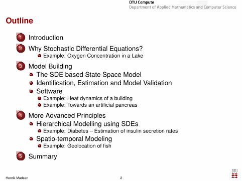
Outline

1 Introduction2 Why Stochastic Differential Equations?

Example: Oxygen Concentration in a Lake

3 Model BuildingThe SDE based State Space ModelIdentification, Estimation and Model ValidationSoftware

Example: Heat dynamics of a buildingExample: Towards an artificial pancreas

4 More Advanced PrinciplesHierarchical Modelling using SDEs

Example: Diabetes – Estimation of insulin secretion rates

Spatio-temporal ModelingExample: Geolocation of fish

5 Summary

Henrik Madsen 2

Introduction

Various methods of advanced modelling are needed for anincreasing number of complex technical, physical, chemical andbiological systems.

For a model to describe the future evolution of the system, itmust

1. capture the inherently non-linear behavior of the system.2. provide means to accommodate for noise due to approximations

and measurement errors.

Calls for methods that are capable of bridging the gap betweenphysical and statistical modelling.

Henrik Madsen 3

Introduction to SDEs

Often systems are described by either1. a set of Ordinary Differential Equations (ODEs) - or2. a set of Stochastic Differential Equations (SDEs)

Solutions to ODEs are deterministic functions (of time). Solutionsto SDEs are stochastic processes.

Henrik Madsen 4

Problem Scenario

Ordinary differential equation

dA = −KA dt

Y = A + ε

Henrik Madsen 5

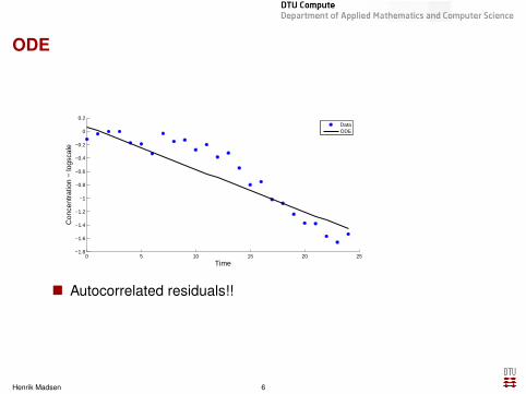
ODE

0 5 10 15 20 25−1.8

−1.6

−1.4

−1.2

−1

−0.8

−0.6

−0.4

−0.2

0

0.2

Time

Con

cent

ratio

n −

logs

cale

DataODE

Autocorrelated residuals!!

Henrik Madsen 6

Problem Scenario

Stochastic differentialequation

dA = −KA dt + dw

Y = A + e

Henrik Madsen 7

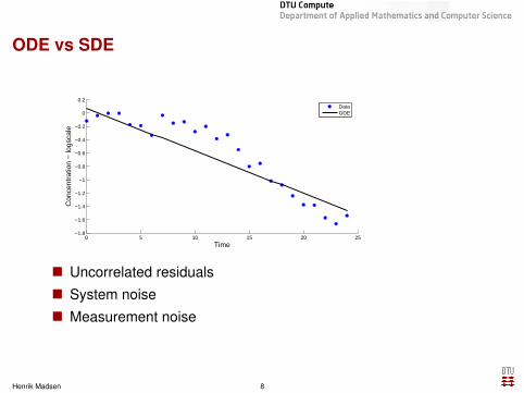
ODE vs SDE

0 5 10 15 20 25−1.8

−1.6

−1.4

−1.2

−1

−0.8

−0.6

−0.4

−0.2

0

0.2

Time

Con

cent

ratio

n −

logs

cale

DataODE

Uncorrelated residuals System noise Measurement noise

Henrik Madsen 8

ODE vs SDE

0 5 10 15 20 25−1.8

−1.6

−1.4

−1.2

−1

−0.8

−0.6

−0.4

−0.2

0

0.2

Time

Con

cent

ratio

n −

logs

cale

DataODESDE

Uncorrelated residuals System noise Measurement noise

Henrik Madsen 8

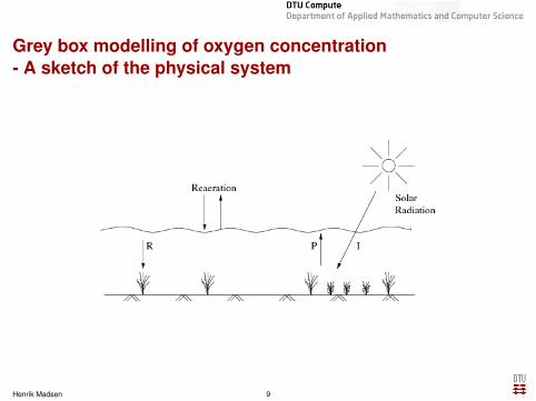
Grey box modelling of oxygen concentration- A sketch of the physical system

Henrik Madsen 9

Grey box modelling of oxygen concentration- A white box model

Model found in the literature:

dCdt

=K

h√

h(Cm(T )− C) + P(I)− R(T )

P(I) = PmE0I

Pm + E0I(= βI)

R(T ) = R15θT−15 [mg/l]

Cm(T ) = 14.54− 0.39T + 0.01T 2 [mg/l]

Simple - however, a non-linear model. Uncertainty of the predictions are not described (or does not

depend on horizon).

Henrik Madsen 10

Grey box modelling of oxygen concentration- A black box model

Box-Jenkins (ARX-model):

Ct − φCt−1 = ωPt + ω0 + εt

Demands equidistant data! Physical interpretation of the parameters is lost!

Henrik Madsen 11

Model validation (first order model)

Henrik Madsen 12

Grey box model of oxygen concentration

The following nonlinear SDE based state space model has beenfound:***The system equation:

[dCdL

]=

[K

h√

h−Kc

K3 −Kl

] [CL

]dt +

[β

√CKbh

0 γ

] [I

Pr

]dt

+

[K

h√

hCm(T )− R(T )

0

]dt +

[dW1(t)dW2(t)

]***The observation equation:

Cr =[1 0

] [CL

]+ e

Henrik Madsen 13

The grey box modelling concept

Combines prior physical knowledge with information in data. The model is not completely described by physical equations, but

equations and the parameters are physically interpretable.

Henrik Madsen 14

Why use grey box modelling?

Prior physical knowledge can be used. Non-linear and non-stationary models are easily formulated. Missing data are easily accommodated. It is possible to estimate environmental variables that are not

measured. Available physical knowledge and statistical modelling tools are

combined to identify parameters of a rather complex dynamicsystem.

The parameters contain information from the data that can bedirectly interpreted by the scientists.

The physical expert and the statistician can collaborate in themodel formulation.

Henrik Madsen 15

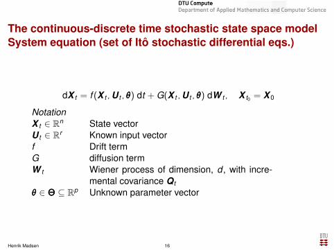
The continuous-discrete time stochastic state space modelSystem equation (set of Itô stochastic differential eqs.)

dX t = f (X t ,U t , θθθ) dt + G(X t ,U t , θθθ) dW t , X t0 = X 0

NotationX t ∈ Rn State vectorU t ∈ Rr Known input vectorf Drift termG diffusion termW t Wiener process of dimension, d , with incre-

mental covariance Qt

θθθ ∈ ΘΘΘ ⊆ Rp Unknown parameter vector

Henrik Madsen 16

Observation equation

The observations are in discrete time, functions of state, input, andparameters, and are subject to noise:

Y ti = h(X ti ,U ti , θθθ) + eti

NotationY ti ∈ Rm Observation vectorh Observation functioneti ∈ Rm Gaussian white noise with covariance ΣΣΣti

Observations are available at the time points ti : t1 < . . . < ti < . . . < tNX 0,W t ,eti assumed independent for all (t , ti ), t 6= ti

Henrik Madsen 17

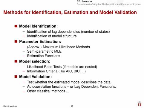
Methods for Identification, Estimation and Model Validation

Model Identification:− Identification of lag dependencies (number of states)− Identification of model structure

Parameter Estimation:− (Approx.) Maximum Likelihood Methods− Semi-parametric MLE− Estimation Functions

Model selection:− Likelihood Ratio Tests (if models are nested)− Information Criteria (like AIC, BIC, ...)

Model Validation:− Test whether the estimated model describes the data.− Autocorrelation functions – or Lag Dependent Functions.− Other classical methods ...

Henrik Madsen 18

Continuous Time Stochastic Modelling (CTSM)

The parameter estimation is performed by using the softwareCTSM.

The software has been developed at DTU Compute. Download from: www.ctsm.info The program returns the uncertainty of the parameter estimates

as well.

Henrik Madsen 19

The estimation procedure (CTSM)

CTSM is based on The Extended Kalman Filter Approximate likelihood estimation

and provides eg. Likelihood testing for nested models Calculations of smoothen state E [X t |YT ]

Calculations of k-step predictions E [X t |Yt−k ].

Henrik Madsen 20

The estimation procedure (CTSM)

CTSM is based on The Extended Kalman Filter Approximate likelihood estimation

and provides eg. Likelihood testing for nested models Calculations of smoothen state E [X t |YT ]

Calculations of k-step predictions E [X t |Yt−k ].

Henrik Madsen 20

Flexhouse layout

Henrik Madsen 21

RC-diagram ofte used for illustrating linear models

Rie

Rie

Rea

Rea

Ti

Ti

Ta

Ta

Te

Te

Φh

Φh

Ci

Ci

Ce

Ce

Henrik Madsen 22

Model A

RiaTi

TaΦh CiAwΦs

Aw is the effective window area.

Henrik Madsen 23

Model Validation for Model A

Autocorrelation function and Periodogram for the residuals.

0 5 10 15 20 25 30 35

−1.

0−

0.5

0.0

0.5

1.0

lag

AC

F

0.0 0.1 0.2 0.3 0.4 0.5

0.0

0.2

0.4

0.6

0.8

1.0

frequency

Model is seen not to be adequate.

Henrik Madsen 24

Model E

After some steps: (Notice that eg. the electric heating system isincluded)

Henrik Madsen 25

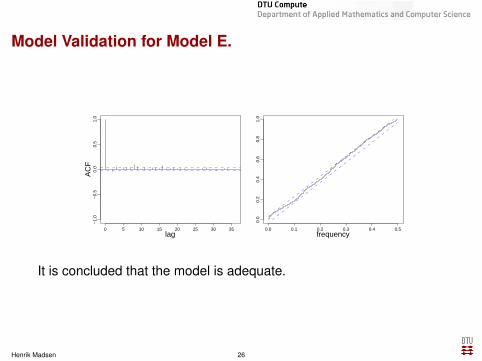
Model Validation for Model E.

0 5 10 15 20 25 30 35

−1.

0−

0.5

0.0

0.5

1.0

lag

AC

F

0.0 0.1 0.2 0.3 0.4 0.5

0.0

0.2

0.4

0.6

0.8

1.0

frequency

It is concluded that the model is adequate.

Henrik Madsen 26

Model for closed loop control

Insulin(subc.)

Insulin(plasma)

Insulineffect

Glucose(plasma)

Intestinalcomp.

Intestinalcomp.

Glucose(int.)

Glucose(subc.)

BLOOD

MealInsulin

CGM

Liver

Henrik Madsen 27

Advanced TopicsHierarchical/Population Modelling – Introduction

Data originating from several population members/subjects Identical experiments Modelling the effect of covariates More data - better estimates of parameters and uncertainties. Software: Population Stochastic Modelling (PSM) or CTSM-R with some extensions - See Juhl et.al. (2015) Software download: www.imm.dtu.dk/psm or

www.ctsm.info

Nonlinear mixed effects model with SDEs

Henrik Madsen 28

Advanced TopicsHierarchical/Population Modelling – Introduction

Data originating from several population members/subjects Identical experiments Modelling the effect of covariates More data - better estimates of parameters and uncertainties. Software: Population Stochastic Modelling (PSM) or CTSM-R with some extensions - See Juhl et.al. (2015) Software download: www.imm.dtu.dk/psm or

www.ctsm.info

Nonlinear mixed effects model with SDEs

Henrik Madsen 28

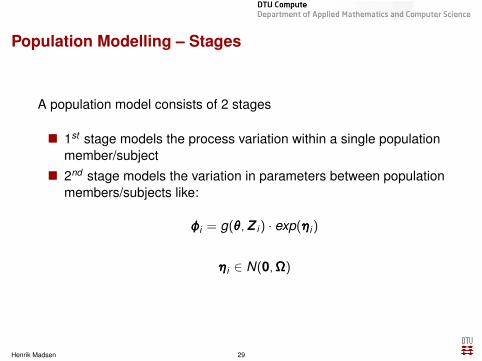
Population Modelling – Stages

A population model consists of 2 stages

1st stage models the process variation within a single populationmember/subject

2nd stage models the variation in parameters between populationmembers/subjects like:

φφφi = g(θθθ,Z i ) · exp(ηηηi )

ηηηi ∈ N(0,ΩΩΩ)

Henrik Madsen 29

Population – Parameter estimation

Parameter estimation using likelihood theory Single member/subject - likelihood based on product of

conditional densities for each time series of length ni (called p1

below). Population likelihood is a combination of the random effects η

and the single member likelihoods

L(θθθ|YNni ) ∝N∏

i=1

∫p1(Yini |φφφi )p2(ηηηi |ΩΩΩ)dηηηi

Henrik Madsen 30

Data – 24H study

12 type 2 diabetic patients Three standardized meals

Henrik Madsen 31

ISR estimate by deconvolution

C-peptide (the observation) is modelled with a 2-compartmentmodel

ISR modelled as a random walk (the third state in x)

dx =

−(k1 + ke) k2 1k1 −k2 00 0 0

x dt + diag

00σISR

dωωω

y = C1 + ε

Henrik Madsen 32

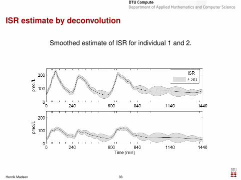
ISR estimate by deconvolution

Smoothed estimate of ISR for individual 1 and 2.

Henrik Madsen 33

Geolocation of Fish

Goal: Learn the structure of fish’movements

GPS systems do not work underwater

’Data storage tages’ formeasuring the pressure (depthunder the surface)

Data gets available at capture ofthe fish

Henrik Madsen 34

Hidden Markov Model

The probabilitiy φ for, that the fish at time t is in position x , is(System equation):

∂φ

∂t= −∇(uφ− D∇φ) (In general)

∂φ

∂t= D

(∂2φ

∂x21

+∂2φ

∂x22

)(Here)

The observations are(Observ. equation):

Yk = Measured pressure/dept at time point tk

Henrik Madsen 35

Hidden Markov Model

The probabilitiy φ for, that the fish at time t is in position x , is(System equation):

∂φ

∂t= −∇(uφ− D∇φ) (In general)

∂φ

∂t= D

(∂2φ

∂x21

+∂2φ

∂x22

)(Here)

The observations are(Observ. equation):

Yk = Measured pressure/dept at time point tk

Henrik Madsen 35

Further physical information

Bathymetry (depths) Time and place for release and

capture Information about the tide system

– see the graph

Henrik Madsen 36

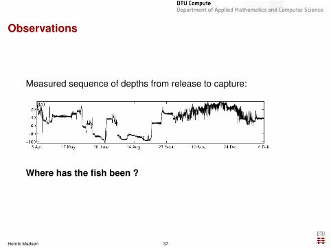
Observations

Measured sequence of depths from release to capture:

Where has the fish been ?

Henrik Madsen 37

Observations

Measured sequence of depths from release to capture:

Where has the fish been ?

Henrik Madsen 37

Geolocation of Fish

Henrik Madsen 38

Summary

By using stochastic differential equations for modelling physical/prior knowledge and information in data are combined,

i.e. we are able to bridge the gap between physical and statisticalmodeling.

we obtain a description of the persistence in the differencesbetween observations and model predictions.

we obtain a rich framework for model identification, estimation,validation and structure modification.

we obtain probabilistic forecasts and simulations.

Henrik Madsen 39

Thanks to:

Jan Kloppenborg Møller Lasse Engbo Christiansen Peder Bacher Anne Katrine Duun-Henriksen Rune Juhl Niels Rode Kristensen Martin Wæver Pedersen Henrik Melgaard

Henrik Madsen 40

Some References - Generic

H. Madsen: Time Series Analysis, Chapman and Hall, 392 pp, 2008.

H. Madsen and P. Thyregod: An Introduction to General and Generalized Linear Models, Chapman and Hall, 340 pp., 2011.

E. Linström, H. Madsen, J.N. Nielsen: Statistics for Finance, Chapman and Hall, 360 pp., 2015.

H.Aa. Nielsen, H. Madsen: A generalization of some classical time series tools, Computational Statistics and Data Analysis, Vol.37, pp. 13-31, 2001.

H. Madsen, J. Holst: Estimation of Continuous-Time Models for the Heat Dynamics of a Building, Energy and Building, Vol. 22, pp.67-79, 1995.

P. Sadegh, J. Holst, H. Madsen, H. Melgaard: Experiment Design for Grey Box Identification, Int. Journ. Adap. Control and SignalProc., Vol. 9, pp. 491-507, 1995.

P. Sadegh, L.H. Hansen, H. Madsen, J. Holst: Input Design for Linear Dynamic Systems using Maxmin Criteria, Journal ofInformation and Optimization Sciences, Vol. 19, pp. 223-240, 1998.

J.N. Nielsen, H. Madsen, P.C. Young: Parameter Estimation in Stochastic Differential Equations; An Overview, Annual Reviews inControl, Vol. 24, pp. 83-94, 2000.

N.R. Kristensen, H. Madsen, S.B. Jørgensen: A Method for systematic improvement of stochastic grey-box models, Computersand Chemical Engineering, Vol 28, 1431-1449, 2004.

N.R. Kristensen, H. Madsen, S.B. Jørgensen: Parameter estimation in stochastic grey-box models, Automatica, Vol. 40, 225-237,2004.

J.B. Jørgensen, M.R. Kristensen, P.G. Thomsen, H. Madsen: Efficient numerical implementation of the continuous-discreteextended Kalman Filter, Computers and Chemical Engineering, 2007.

K.R. Philipsen, L.E. Christiansen, H. Hasman, H. Madsen: Modelling conjugation with stochastic differential equations, Journal ofTheoretical Biology, Vol. 263, pp. 134-142, 2010.

R. Juhl, J.K. Møller, J.B. Jørgensen, H. Madsen: Modeling and Prediction using Stochastic Differential Equations, Springer bookchapter, 2015

Henrik Madsen 41