STOCHASTIC PROCESSES: Introducing Differential Equations · STOCHASTIC PROCESSES: Introducing...
32
STOCHASTIC PROCESSES: Introducing Differential Equations CIS002-2 Computational Alegrba and Number Theory David Goodwin [email protected] 10:00, Monday 12 th March 2012
Transcript of STOCHASTIC PROCESSES: Introducing Differential Equations · STOCHASTIC PROCESSES: Introducing...
STOCHASTIC PROCESSES:Introducing Differential EquationsCIS002-2 Computational Alegrba and Number
Theory
David [email protected]
10:00, Monday 12th March 2012

Introduction Vector DE Writing DE Solving DE Linear DE Vector Linear DE
Outline
1 Introduction
2 Vector Differential Equations
3 Writing Differential Equations usingDifferentials
4 Solving Differential Equations
5 A Linear Differential Equation with Driving
6 Solving Vector Linear Differential Equations
Introduction Vector DE Writing DE Solving DE Linear DE Vector Linear DE
Introducing Differential Equations
• A differential equation is one that involves one or more derivatives of afunction
Example
Say we have a toy train on a straight track, and x is the position of the trainalong the track. If the train is moving then x will be a function of time, x(t).If we apply a constant force (from constant electric power), F , to the train,then its accelaration, being the second derivative of x , is equal to F/m, wherem is the mass of the train. Thus we have a simple differential equation:
d2x
dt2=
F
m
Introduction Vector DE Writing DE Solving DE Linear DE Vector Linear DE
Introducing Differential Equations
• Although an integral can be seen as the area under a plotted curvebetween two limits, it can also be viewed as the inverse of differentiation,where differentiation can be seen as the gradient of a plotted curve at anysingle point.
• The pneumonic is “add one to the power and divide by the new power”for the integral of simple powers. Integration is accurate up to anarbritrary constant of integration, which can be thought of as commingfrom the y-intercept of the plot.
Example
To find how x varies with time, we need to find the function x(t) that satisfiesthe previous differential equation. Here we can integrate both sides of theequation twice to recover x :
x(t) =F
2mt2 + v0t + x0
where v0 and x0 come from the constants of integration, and represent theinitial velocity and initial position of the toy train.
Introduction Vector DE Writing DE Solving DE Linear DE Vector Linear DE
Outline
1 Introduction
2 Vector Differential Equations
3 Writing Differential Equations usingDifferentials
4 Solving Differential Equations
5 A Linear Differential Equation with Driving
6 Solving Vector Linear Differential Equations
Introduction Vector DE Writing DE Solving DE Linear DE Vector Linear DE
Vector Differential Equations
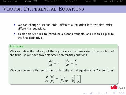
• We can change a second order differential equation into two first orderdifferential equations.
• To do this we need to introduce a second variable, and set this equal tothe first derivative.
Example
We can define the velocity of the toy train as the derivative of the position ofthe train, so we have two first order differential equations.
dx
dt= v
dv
dt=
F
m
We can now write this set of first order differential equations in “vector form”.
d
dt
[xv
]=
[0 1
F/mx 0
] [xv
]

Introduction Vector DE Writing DE Solving DE Linear DE Vector Linear DE
Vector Differential Equations
Example
Defining x = (x , v)T and A as the matrix
A =
[0 1
F/mx 0
]We can now write the set of equations in compact form
x ≡ dx
dt= Ax
If the elements of the matrix A do not depend on x, then this equation wouldbe a linear first-order vector differential equation.
Introduction Vector DE Writing DE Solving DE Linear DE Vector Linear DE
Outline
1 Introduction
2 Vector Differential Equations
3 Writing Differential Equations usingDifferentials
4 Solving Differential Equations
5 A Linear Differential Equation with Driving
6 Solving Vector Linear Differential Equations
Introduction Vector DE Writing DE Solving DE Linear DE Vector Linear DE
Vector Differential Equations
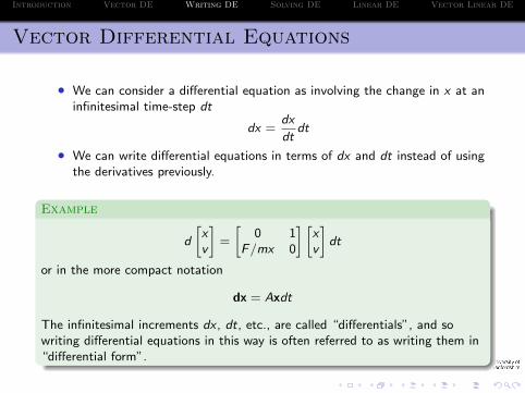
• We can consider a differential equation as involving the change in x at aninfinitesimal time-step dt
dx =dx
dtdt
• We can write differential equations in terms of dx and dt instead of usingthe derivatives previously.
Example
d
[xv
]=
[0 1
F/mx 0
] [xv
]dt
or in the more compact notation
dx = Axdt
The infinitesimal increments dx , dt, etc., are called “differentials”, and sowriting differential equations in this way is often referred to as writing them in“differential form”.

Introduction Vector DE Writing DE Solving DE Linear DE Vector Linear DE
Outline
1 Introduction
2 Vector Differential Equations
3 Writing Differential Equations usingDifferentials
4 Solving Differential Equations
5 A Linear Differential Equation with Driving
6 Solving Vector Linear Differential Equations
Introduction Vector DE Writing DE Solving DE Linear DE Vector Linear DE
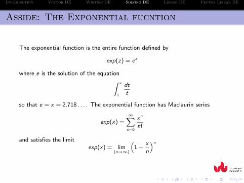
Asside: The Exponential fucntion
The exponential function is the entire function defined by
exp(z) = ez
where e is the solution of the equation∫ x
1
dt
t
so that e = x = 2.718 . . . . The exponential function has Maclaurin series
exp(x) =∞∑n=0
xn
n!
and satisfies the limitexp(x) = lim
(n→∞)
(1 +
x
n
)n
Introduction Vector DE Writing DE Solving DE Linear DE Vector Linear DE
An Alternative method for solvingdifferential equations
• Consider the simple linear differential equation dx = −γxdt.
• This tells us that the value of x at time t + dt is the value at time t plusdx .
• x(t + dt) = x(t) − γx(t)dt = (1 − γ)x(t)
• To solve this we note that to first order in dt (that is, when dt is verysmall) eγdt ≈ 1 + γdt. This comes from the definition of ex
(ex =∑∞
n=0xn
n!= 1 + x + x2
2!+ x3
3!+ x4
4!+ · · · .)
• This changes our equation to x(t + dt) = e−γdtx(t), which tells us thatto move x from time t to t + dt we simple multiply x(t) by e−γdt .
• To move two lots of dt we simple multiply this factor twice. To move tosome arbitrary time x(t + τ) all we do is apply this relation repeatedly.
• Let us say that dt = τ/N for some large N.
x(t + τ) =(e−γdt
)Nx(t) = e−γNdtx(t) = e−γτx(t)
• The equation solved above is the simplest linear differential equation.
Introduction Vector DE Writing DE Solving DE Linear DE Vector Linear DE
Outline
1 Introduction
2 Vector Differential Equations
3 Writing Differential Equations usingDifferentials
4 Solving Differential Equations
5 A Linear Differential Equation with Driving
6 Solving Vector Linear Differential Equations
Introduction Vector DE Writing DE Solving DE Linear DE Vector Linear DE
A Linear Differential Equation with Driving
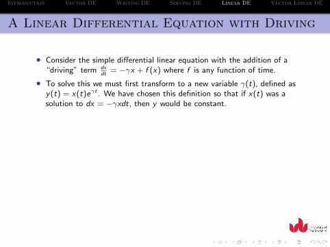
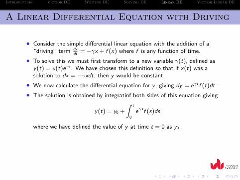
• Consider the simple differential linear equation with the addition of a“driving” term dx
dt= −γx + f (x) where f is any function of time.
• To solve this we must first transform to a new variable γ(t), defined asy(t) = x(t)eγt . We have chosen this definition so that if x(t) was asolution to dx = −γxdt, then y would be constant.
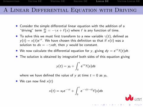
• We now calculate the differential equation for y , giving dy = eγt f (t)dt.
• The solution is obtained by integratinf both sides of this equation giving
y(t) = y0 +
∫ t
0
eγs f (s)ds
where we have defined the value of y at time t = 0 as y0.
• We can now find x(t)
x(t) = x0e−γt +
∫ t
0
e−γ(t−s)f (s)ds
Introduction Vector DE Writing DE Solving DE Linear DE Vector Linear DE
A Linear Differential Equation with Driving
• Consider the simple differential linear equation with the addition of a“driving” term dx
dt= −γx + f (x) where f is any function of time.
• To solve this we must first transform to a new variable γ(t), defined asy(t) = x(t)eγt . We have chosen this definition so that if x(t) was asolution to dx = −γxdt, then y would be constant.
• We now calculate the differential equation for y , giving dy = eγt f (t)dt.
• The solution is obtained by integratinf both sides of this equation giving
y(t) = y0 +
∫ t
0
eγs f (s)ds
where we have defined the value of y at time t = 0 as y0.
• We can now find x(t)
x(t) = x0e−γt +
∫ t
0
e−γ(t−s)f (s)ds
Introduction Vector DE Writing DE Solving DE Linear DE Vector Linear DE
A Linear Differential Equation with Driving
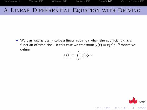
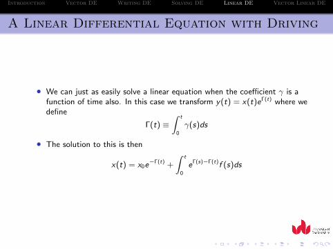
• We can just as easily solve a linear equation when the coefficient γ is afunction of time also. In this case we transform y(t) = x(t)eΓ(t) where wedefine
Γ(t) ≡∫ t
0
γ(s)ds
• The solution to this is then
x(t) = x0e−Γ(t) +
∫ t
0
eΓ(s)−Γ(t)f (s)ds
Introduction Vector DE Writing DE Solving DE Linear DE Vector Linear DE
A Linear Differential Equation with Driving
• We can just as easily solve a linear equation when the coefficient γ is afunction of time also. In this case we transform y(t) = x(t)eΓ(t) where wedefine
Γ(t) ≡∫ t
0
γ(s)ds
• The solution to this is then
x(t) = x0e−Γ(t) +
∫ t
0
eΓ(s)−Γ(t)f (s)ds
Introduction Vector DE Writing DE Solving DE Linear DE Vector Linear DE
Outline
1 Introduction
2 Vector Differential Equations
3 Writing Differential Equations usingDifferentials
4 Solving Differential Equations
5 A Linear Differential Equation with Driving
6 Solving Vector Linear Differential Equations
Introduction Vector DE Writing DE Solving DE Linear DE Vector Linear DE
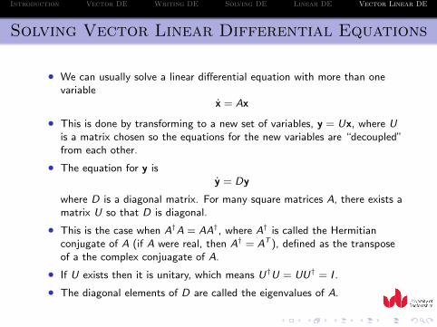
Solving Vector Linear Differential Equations
• We can usually solve a linear differential equation with more than onevariable
x = Ax
• This is done by transforming to a new set of variables, y = Ux, where Uis a matrix chosen so the equations for the new variables are “decoupled”from each other.
• The equation for y isy = Dy
where D is a diagonal matrix. For many square matrices A, there exists amatrix U so that D is diagonal.
• This is the case when A†A = AA†, where A† is called the Hermitianconjugate of A (if A were real, then A† = AT ), defined as the transposeof a the complex conjuagate of A.
• If U exists then it is unitary, which means U†U = UU† = I .
• The diagonal elements of D are called the eigenvalues of A.
Introduction Vector DE Writing DE Solving DE Linear DE Vector Linear DE
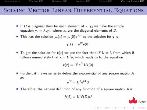
Solving Vector Linear Differential Equations
• If D is diagonal then for each element of y , yn we have the simpleequation yn = λnyn, where λn are the diagonal elements of D.
• This has the solution yn(t) = yn(0)eλnt so the solution for y is
y(t) = eDty(0)
• To get the solution for x(t) we use the fact that U†U = I , from which iffollows immediately that x = U†y, which leads us to the equation
x(t) = U†eDtUx(0)
• Further, it makes sense to define the exponential of any square matrix Aas
eAt = U†eDtU
• Therefore, the natural definition of any function of a square matrix A is
f (A) ≡ U†f (D)U
Introduction Vector DE Writing DE Solving DE Linear DE Vector Linear DE
Summary
To summarise the above results, the solution to the vector differential equation
x = Ax
isx(t) = eAtx(0)
whereeAt = U†eDtU
We can also solve any linear vector differential equation with driving, just as wedid for thwe single variable linear equation.