Modelling the Underwriting Cycleby René Schnieper

Lavaterstr. 51, 8002 Zurich, Switzerlandreneschnieper@dplanet.ch

Abstract

A model of the insurance market is proposed which enables a better under-standing of underwriting cycles. Price and quantity of insurance are determinedby the equilibrium of supply and demand. Supply is driven by the amount ofequity available to insurance companies. Pro�ts an losses feed back into surplusleading to �uctuations in returns. The in�uence of accounting and regulatoryissues on the emergence of pro�t is taken into account. A generalization ofthe model is obtained by assuming that the pro�t in any given �scal year is arandom variable. A further generalization is proposed which allows for capitalin�ows and out�ows in excess of retained earnings and losses.In general market price and quantity are de�ned by an implicit equation

which must be solved numerically. The capital of individual suppliers is de�nedby a system of di¤erence equations. A simpli�ed version of the model leads toan explicit solution for equilibrium price and quantity. The aggregate marketcapital is de�ned by a linear di¤erence equation with constant coe¢ cients. Thebehaviour of solutions is analyzed.The literature on underwriting cycles is reviewed. Within the context of our

model it is possible to analyze the impact of di¤erent contributing factors andtheir interaction in an integrated framework. This leads to a better understand-ing of underwriting cycles.

Keywords

Underwriting cycle, insurance market, supply, demand, market equilibrium,market price, market quantity, di¤erence equations, stability, equilibrium points,time series, stationarity, autoregressive processes.

1 The General Model

1.1 Introduction

Practitioners all experience the cyclical nature of insurance markets. Periodsof low, sometimes even negative returns alternate with periods of high pro�ts.The characteristics of the cycle, its length, its amplitude, etc. vary betweenmarket segments - e.g. private lines and commercial lines - between geographicalmarkets and over time. Cycles however, are a universal feature of insurancemarkets.Di¤erent theories have been proposed to explain the cyclical nature of in-

surance pro�ts. In section 1.2 we review some of this material. In section 1.3and 1.4 we propose our own model which is based on the assumption that cy-cles stem from changes in supply of and demand for insurance. The insurance

1

supply is de�ned by insurance providers who are characterized by their amountof capital, their targeted return on capital and their supply elasticity i.e. the�exibility with which they respond to market returns in excess or below theirown target returns. Similarly the demand for insurance is de�ned by insurancebuyers who are characterized by their individual base demand for insurance andtargeted returns on capital. The demand elasticity is a further characteristicof each individual buyer. For each period equilibrium price and equilibriumquantity result from the intersection of supply and demand curves. The priceof insurance, i.e. the rate of return on risk based capital, is equal to the rateof return which clears the market i.e. to that rate of return for which o¤er anddemand are equal. The quantity of insurance transacted during a given period,i.e. the amount of pure risk premium underwritten during that period, is equalto the quantity corresponding to the equilibrium rate of return. The net pro�tafter taxes and dividends is reinvested. Pro�ts and losses feed into surplus,leading to o¤setting changes in supply. Base demand increases according togrowth rates which are driven by the economic cycle leading to further shifts inmarket equilibrium. Underwriting cycles are thus driven by features which lieat the heart of the insurance business.The speed with which pro�ts and losses emerge can exacerbate or dampen

underwriting cycles. Accounting factors and regulatory constraints thus havean impact on underwriting cycles. In a more re�ned version of the model capital�ows in and out of the market are taken into account. The model also allowsan analysis of the consequences of supply and demand shifts stemming fromshocks such as catastrophe losses, industry-wide, sharp increases in loss reserves,signi�cant changes in the value of assets, redirection of business to insurancecaptives or risk retention groups, etc.The theory of di¤erence equations as well as the theory of time series provide

valuable insights into the behaviour of insurance markets. The focus of thearticle is on di¤erence equations rather than on time series, i.e. on expectedvalues rather than on realizations of random variables. However equilibriumpoints and characteristic roots are of relevance to both di¤erence equations andtime series. The di¤erence equation models proposed in the article can begeneralized in a straightforward way to time series models.

1.2 Related Literature

Many studies have addressed the issue of cyclical underwriting returns and haveproposed competing theories to explain the phenomenon. important contribu-tions include the ones mentioned below.The irrational-expectation hypothesis by E. Venezian (1985): the author

proposes a model for rate-making. Future loss costs are estimated based onhistorical loss costs using a regression analysis. Venezian shows that the random�uctuations contained in past loss costs lead to future underwriting results whichare autocorrelated. The theory is supported by empirical evidence. The authoranalyses the performance of thirteen lines of business in the US P&C insuranceindustry between 1960 and 1980. He shows that the pro�t margins of eleven lines

2

are best described by and autoregressive process of order two (AR(2) process).The �tted AR(2) processes are all stationary and cyclical.The rational-expectations / institutional intervention hypothesis by J.D.

Cummins and J. F. Outreville (1987): the authors postulate that cycles arecreated in an otherwise rational market through institutional, regulatory andaccounting factors. The authors assume that the subjective expected valuesof future losses are equal to the objective expectations based on informationavailable at the time rates are established. Data collection lags, regulatory lags,policy renewal lags and lags due to accounting rules lead to cyclicality in under-writing results. The data from thirteen countries for the period 1957 to 1979 isanalyzed. In most countries there is evidence of cyclicality and the best �t isprovided by an AR(2) process. The �ndings are con�rmed by J. Lamm-Tennantand M.A. Weiss (1997).The feedback of pro�t and losses into surplus postulated by L. A. Berger

(1988) is a further attempt at explaining the cyclical nature of underwritingreturns. Berger provides a fully �edged model of the underwriting cycle. Themarket for insurance is modelled by standard supply and demand theory. Equi-librium price and quantity result from the equilibrium of supply and demand.Pro�ts and losses feed into surplus leading to shifts in supply which o¤set thepro�t or loss trend. The behaviour of the model is consistent with usual cycletheory. The capacity-constraint hypothesis by R. Winter (1988) emphasizes aspecial feature of the above theory. Winter suggests that insurers will not imme-diately adjust surplus when it is reduced by external shocks because in adversecircumstances, external equity is expensive. This leads prices to increase wheninsurance capacity or equity is reduced.The change-in-expectations hypothesis of G. Lai and R. C. Whitt (1992) and

of G. Lai et al. (2000) postulates that increased uncertainty in particular aboutloss costs leads to higher premiums. Lai et al. propose an economic model ofthe insurance market. Suppliers and buyers are characterised by their utilityfunctions. Insurance price is derived from market equilibrium. Under certainassumptions an explicit formula is derived for insurance price and quantity. Itis shown that prices increase when the variance of losses increases.External factors are invoked as an explanation for the underwriting cycle.

M. F. Grace and R. E. Hoyt (1995) �nd a long-run relationship between generaleconomic changes and underwriting performance. N. A. Doherty and B. Kang(1988) suggest that �uctuation in interest rates create insurance pricing cycles.A certain number of articles rely on data analysis alone to investigate the de-

terminants of insurance prices. For instance M. A. Weiss and J.-H. Chung (2004)perform a multiple regression analysis with the price of US non-proportionalreinsurance as the dependent variable. They �nd that capital strength andoverall capacity are signi�cant factors determining reinsurance prices.

3

1.3 Market Equilibrium

1.3.1 Supply

Let us �rst assume that there is only one company selling insurance. Let Cdenote the amount of capital of the company. Let P denote the pure riskpremium corresponding to the amount of insurance sold by the company (i.e. theexpected loss costs on an undiscounted basis). We refer to P as to the quantityof insurance. It is assumed that the amount of risk based capital necessaryto underwrite P is equal to P

�s where �s is the leverage of the company. The

company is further characterized by the following quantities: rs is the targetrate of return on risk based capital and �s is the supply elasticity. The exactmeaning of the last two parameters becomes clear in the light of the supplyfunction de�ned below. Finally let r be the rate of return on risk based capitalachieved in the market. This quantity is referred to as the price of insurance.It is assumed that the following relation holds true between the quantity ofinsurance (P) and the price of insurance (r)

P = �sC + �s(r � rs) P�s:

�sC is the base supply, i.e. that quantity of insurance which is provided whenthe market rate of return on risk based capital (r) is equal to the target rateof return of the supplier (rs). rs P�s is the loading required by the supplier forassuming the quantity of insurance risk P. r P�s is the loading e¤ectively achievedin the market. (r � rs) P�s is thus the economic value added. It is reasonableto assume that the amount of insurance provided in excess of the base supply(P ��sC) is proportional to the economic value added, where the elasticity �s isthe proportionality factor. Hence the above relation between insurance quantityand insurance price. Expressing quantity as a function of price, we obtain

P =�sC

1� �s

�s (r � rs):

The supply function is usually de�ned as the inverse function

r = rs +�s

�s(1� �sC

P)

where price is expressed as a function of quantity.Note that both rates of return r and rs apply to the risk based capital P

�s

and not to the e¤ective amount of capital C. It is assumed that the owners ofthe company de�ne the rate of return in terms of the e¤ective risk they assume.This is realistic as long as the risk based capital is not signi�cantly larger thanthe e¤ective capital.

1.3.2 Demand

Let us �rst consider commercial insurance buyers. For the time being we assumethat there is only one company buying insurance. As in the previous section,

4

let P , the pure risk premium, denote the quantity of insurance bought. It isassumed that the amount of capital allocated by the buyer to the insurancerisk is equal to P

�dwhere �d is the leverage of the buyer. The buyer is further

characterized by the following quantities: P 0 the base demand, rd the costof capital and �d the demand elasticity. The fair loading which the buyer isprepared to pay in excess of the expected loss costs P is thus equal to rd P

�d.

The loading required by the market is r P�s :It is thus reasonable to assume thatthe following relation holds true between the quantity of insurance bought (P )and the price of insurance (r)

P = P 0 � �d( r�s� rd

�d)P

Introducing the modi�ed target rate of return of the buyer

rd0

= rd�s

�d

we obtain a similar equation as for the supply side

P = P 0 � �d(r � rd0

)P

�s:

The quantity of insurance bought is given by the following function of price

P =P 0

1 + "d

�s (r � rd0)=

P 0

1 + �d( r�s �rd

�d)

and the demand function is

r = rd0

+�s

�d(P 0

P� 1) = rd

�s

�d+�s

�d(P 0

P� 1):

In the case of private insurance buyers it is assumed that buyers price risksaccording to the expected value principle and that they all use the same loading.Let P 0 denote the aggregate base demand. Let P denote the aggregate demandand let �P denote the fair loading from the buyers�viewpoint. Assume that allbuyers have the same demand elasticity �d. We have

P = P 0 � �d(r P�s� �P ) = P 0 � �d(r � rd

�)P

�s

with rd�= ��s, which is of the same form as the equation we have obtained

for commercial buyers.

1.3.3 Equilibrium Price and Quantity

The equilibrium price and the equilibrium quantity result from the intersectionof the supply and of the demand curve. By equating the insurance quantity

5

bought, respectively sold, expressed as a function of price, we obtain the equi-librium price rm

rm =(�dC)rd

0+ (�s P

0

�s )rs

�dC + �s P0

�s

+P 0 � �sC�dC + �s P

0

�s

(1.3.3.1)

The market rate of return is a weighted average of the supply target rate ofreturn and of the modi�ed demand target rate of return plus a correction termdepending on the excess of base demand over base supply.By equating the price as expressed in the supply respectively in the demand

function one derives the equilibrium insurance quantity Pm

Pm =�sP 0 + �d(�sC)

�s + �d + �s�d( rs

�s �rd

�d)

(1.3.3.2)

The equilibrium quantity is a weighted average of the base demand and of thebase supply with an additional term in the denominator which depends on thedi¤erence in targeted return on sales of buyers and sellers.

The equilibrium loading is

�m = rmPm

�s=(�drd

0� �s)C + (1 + �s rs�s )P

0

�s + �d + �s�d( rs

�s �rd

�d)

(1.3.3.3)

The fact that the expression for the loading simpli�es will prove to be usefullater.

1.3.4 Retained Earnings and Capital Growth

It is assumed that the amount of capital of the company in the next period(Ct+1) is equal to the amount of capital in the current period (Ct) plus a shareof the equilibrium loading generated during the current period (�mt ) plus a shareof the return on capital generated by the �nancial risk of the company (rfCt):Let�t denote the share of the earnings which is contributed to the capital of thenext period. (1 � �t is the share of the earnings which is paid out as taxesand dividends.) The capital of the company in the next period is given by thefollowing formula

Ct+1 = Ct + �trfCt + �t�

mt (1.3.3.4)

We assume that the accounting is based on economic value, i.e. that assetsand liabilities are marked to market. �mt is the insurance operating return. Itis the expected net present value of premiums less claims payments discountedto the middle of the period. Costs are not taken into account. rfCt is theexpected return on capital generated by the �nancial risk of the company. It

6

stems from the investment income generated by the assets matching the capitaland from any excess return generated by a possible mismatch between assetsand liabilities. In section 3.1, we broaden the de�nition of this risk. For thetime being we ignore random �uctuations around expected values. For moredetails on the model see R. Schnieper [2000].

1.4 The General Model

From now on we consider a multi-period model. (Typically a period is a yearbut other units of time can be considered: months, quarters, etc.) We assumethat both the supply side and the demand side of the market consist of manyparticipants.An insurance market consists of a certain number of suppliers and of a

certain number of insurance buyers. It is assumed that the suppliers specializein providing insurance to the said group of buyers and that the buyers essentiallyonly buy from the said group of suppliers. Examples of insurance marketsare: the Swiss, the French or the UK personal lines market, the internationalmarket for large corporate risks, the worldwide reinsurance market. Whilstcertain insurance groups are active in many such markets, we focus on thoselegal entities or departments within the group which are dedicated to a speci�cmarket.Let Ck;t denote the amount of capital of company k at the beginning of

period t: It is assumed that base demand of all buyers increases by a factor tduring period t; therefore base demand of buyer l at the beginning of period tis

P 0l;t = 0 � 1 � ::: � t�1 � P 0l = �t � P 0lwhere

�t = 0 � 1 � ::: � t�1:The amount of insurance sold by company k during period t is de�ned by

Pk;t = �s � Ck;t + "sk(r � rsk) �Pk;t�s

(1.4.1)

and the amount of insurance bought by buyer number l during period t is de�nedby

Pl;t = �t � P 0l � "dl (r

�s� rdl�dl) � Pl;t (1.4.2)

Note that the leverage factors, the target rates of return as well as the elasticitiesare time independent. Note that the leverage factor of the supply side of themarket is the same for all suppliers i.e. there is a market consensus about theamount of risk based capital necessary to write a given quantity of pure riskpremium. The market equilibrium for period t is reached for that value of r forwhich aggregate supply and aggregate demand are equal

nsXk=1

�sCk;t

1� "sk�s (r � rsk)

=

ndXl=1

�tP0l

1 + "dl (r�s �

rdl�dl)

(1.4.3)

7

Let rmt denote the solution of this equation. (It is easily seen that the aboveequation admits exactly one solution.) rmt is the market rate of return achievedduring period t: Let P sk;t denote the amount of insurance sold by supplier kduring period t. It is derived by solving (1.4.1) for Pk;t and by inserting rmt forr. The amount of pro�t made by company k during period t

�sk;t = rmtP sk;t�s

=rmt Ck;t

1� "sk�s (r

mt � rsk)

Let �k;t denote the pro�t retention rate of company k at the end of period t.

Let rfk denote the rate of return generated by the �nancial risk of company kincluding the return on assets matching the equity. Let us also assume thatcompany k does not return any capital in addition to the dividend or obtainany capital increase in addition to the retained earnings. Company k�s capitalat the beginning of period t+ 1 is thus

Ck;t+1 = Ck;t + �k;trfkCk;t + �k;t�

sk;t

Ck;t+1 = Ck;t(1 + �k;trfk +

�k;trmt

1� "sk�s (r

mt � rsk)

) k = 1; :::; ns (1.4.4)

On the other hand, the base demand from buyer l at the beginning of periodt+ 1 is

P 0l;t+1 = �t+1 � P 0l ; l = 1; :::; n�:

and it is seen that if we specify the starting capital of each company

Ck;0 for k = 1; :::; ns

the system of di¤erence equations (1.4.4) together with the implicit equation(1.4.3) for the market rate of return enables us to compute the capital of eachcompany at the beginning of each period together with the achieved marketrate of return in each period. Examples are given below. No general statementcan be made about the behaviour of the solution of this system of di¤erenceequations since it depends on unspeci�ed time-varying pro�t retention ratesand demand growth rates.An interesting special case arises when these quantities are time independent.

Let t= for all t, hence

�t = t

We also assume�k;t = �k for all t

We make the following variable changes

Ck;t =Ck;t t and P

0

l;t =P 0l;t

t = P 0lDe�nitions

8

Ck;t is the standardized capital of company k at the beginning of periodt and P

0

l;t = P 0l is the standardized base demand of buyer l.The market rate of return during period t; rmt ; is the solution of the following

equation

nsXk=1

�sCk;t

1� "sk�s (r � rsk)

=

ndXl=1

P 0l

1 + "dl (r�s �

rdl�dl)

(1.4.3a)

and company k0s standardized capital at the beginning of period t + 1 isgiven by the following di¤erence equation

Ck;t+1 = Ck;t1

(1 + �kr

fk +

�krmt

1� "sk�s (r

mt � rsk)

) k = 1; ::::; ns (1.4.4a)

The following de�nition is borrowed from the theory of di¤erence equations(See e.g. S.M. Elaydi [1999])De�nition(C1; :::; Cns ; r

m) is an equilibrium point of the system of di¤erence equations(1.4.3a) and (1.4.4a) if and only if

Ck;t0 = Ck k = 1; ::::; nsrmt0 = rm

g ) Ck;t = Ck k = 1; ::::; nsrmt = rm

g for all t � t0

TheoremFor time-homogeneous pro�t retention rates and demand growth rates(i) There exists an equilibrium point (C1; :::; Cns ; r

m) of the system of equa-tions (1.4.3a) and (1.4.4a). It is characterized by the fact that Ck 6= 0 for exactlyone value of k.(ii) Let k0 denote the value of k for which Ck 6= 0; the equilibrium rate of

return is given by the following equation

rm =

1rsk0

+"sk0�s

�k0 �1��kr

fk

+"sk0�s

rsk0

ProofFrom the de�nition of the equilibrium point and from (1.4.4.a) we obtain

�krm

1 +"sk�s (r

m � rsk)= � 1� �kr

fk

for all k for which Ck 6= 0: Hence if k is such that Ck 6= 0; we obtain

rm =1 +

"sk�s r

sk

�k �1��kr

fk

+"sk�s

9

Without loss of generality it can be assumed that the right hand side of theabove equation is di¤erent for di¤erent values of k:(If this is not the case, oneaggregates the suppliers with identical values.) Hence Ck 6= 0 for at most onevalue of k. Ck = 0 for all values of k is the degenerate case which is only achievedif the capital of all suppliers is zero Hence Ck 6= 0: for exactly one value of k.Which proves (i) and (ii)

Q.E.D.Remarks1. The statement of the above theorem is an argument in favour of a homo-

geneous supply side of the market, i.e. of a model where all suppliers have thesame target rate of return and elasticity. In such a case, the supply side behavesas one single seller with a capital equal to the aggregate capital of the market.In most insurance markets, the demand side consists of a large number of moreor less homogeneous buyers. Assuming the same target rate of return, leverageand elasticity for all buyers is therefore realistic. In such a case, the demandside of the market also behaves as one single buyer with a base demand equalto the aggregate base demand of the market.2. In those cases where market participants are heterogeneous, it can be

shown that a suitably de�ned single buyer and single seller model provides agood approximation to the more complex market in the sense that both equilib-rium price and quantity of the approximating model are not too di¤erent fromequilibrium price and quantity of the original model. The approximating singlebuyer and single seller model is obtained by de�ning the leverage, target rate ofreturn and elasticity as weighted averages. The weights on the supply side areequal to the capital of individual sellers. On the demand side the weights areequal to the base demand of each buyer.

1.5 Examples

1.1 The supply side of the market consists of two groups of sellers with �s = 2:5and �s = 5 for both groups and rs1 = 10% and r

s2 = 6% respectively. It is further

assumed that C1;0 = 50 [Monetary Unit] and C2;0 = 50 [MU].The demand side of the market consists of one group of homogeneous buyers

with �d = 2:5; �d = 5 and rd = 8%:It is further assumed that P 0 = 200:Since �s = 2:5; the choice of C0 = C1;0+C2;0 = 100 and of P 0 = 200 means

that there is a supply overcapacity. In addition we assume rf = 2% and � = 0:5for all suppliers and = 1:05:Applying (1.4.3a) and (1.4.4a) we have computed the values of the stan-

dardized variables. For comparison purposes we have also tabulated the valuesof the standardized variables of the approximating homogeneous model withrs1 =

s2= 0:08%: The results are summarized in the following table

10

Inhomogeneous Model Homogeneous Modelt Ct [MU] rmt [%] Ct [MU] rmt [%]0 100 2:41 100 2:441 97:2 3:11 97:2 3:142 94:8 3:72 94:9 3:755 89:5 5:17 89:5 5:1910 84:4 6:60 84:5 6:6220 80:9 7:66 81:0 7:6830 80:1 7:90 80:2 7:93Over the above range, the approximation of the inhomogeneous model by the

corresponding homogeneous model is excellent. The values are nearly identical.The results seem to converge. However, if we compute the solution of the systemof di¤erence equations for a much longer period, we obtain

Inhomogeneous Model Homogeneous Modelt Ct [MU] rmt [%] Ct [MU] rmt [%]100 79:6 7:94 80 8:00200 79:3 7:90 80 8:00500 78:5 7:82 80 8:001000 77:9 7:75 80 8:00For practical purposes a period of such length is meaningless. It is however

interesting to notice that the solutions of the system of di¤erence equationscorresponding to the inhomogeneous model no longer seem to converge.It is also interesting to notice that the relative weight - measured by relative

equity - of the �rst group of suppliers decreases from 50% (t=0) to 48% (t=30)to 43% (t=100) and to 5% (t=1000).The process corresponding to the inhomogeneous model consists of an over-

lap of two trends: (i) Standardized equity decreases in order to adjust to lowerbase demand. As a consequence the rate of return increases. (ii) Over a verylong period of time, the process seems to converge towards the equilibriumpoint described in the theorem of section 1.4. For practical purposes however,the latter trend is irrelevant.1.2 Model parameters are as in model 1.1 except for the following two dif-

ferences P 0 = 250 and = 1:04:i.e. the starting capital and base demand are inbalance but targeted net capital growth rate is higher than base demand growthrate. We obtain the following values

t Inhomogeneous Model Homogeneous ModelCt [MU] rmt [%] Ct [MU] rmt [%]

0 100 7.96 100 8.001 100.9 7.72 101.0 7.762 101.8 7.52 101.8 7.555 103.6 7.06 103.7 7.0910 105.5 6.62 105.6 6.6520 106.8 6.30 106.9 6.3230 107.1 6.22 107.3 6.24As in the preceding example, the approximation of the inhomogeneous model

by the corresponding homogeneous model is excellent. As t grows larger, we ob-

11

tain for the homogeneous model Ct ! 107:4 and rmt ! 6:21%:The unbalancebetween the two above mentioned growth rates leads to a slight capacity over-supply and to a corresponding decrease in the rate of return.1.3Model parameters are as in model 1.1 except for the following di¤erences

P 0 = 250 and demand growth is assumed to be cyclical. The average growthfactor is assumed to be = 1:05 as in 1.1 above, however it is assumed thatduring the �rst two periods there is an excess growth of base demand of 5%,followed by four periods with a growth de�cit of 5% and �nally two periods withan excess growth of 5% thus leading to a cycle of length eight. This is modelledby multiplying base demand in the standardized model by the following factors

(�1; :::�8) = (1:05; 1:05; 0:95; 0:95; 0:95; 0:95; 1:05; 1:0606)

The factors are applied in a cumulative way. The last factor has been chosenin a way to ensure that the product of all factors is equal to one. After a fewcycles the process converges. Below we have tabulated the results of the thirdcycle. They do not change much after that.

Base Inhomogenous Model Homogenous Modelt Demand [MU] Ct [MU] rmt [%] Ct [MU] rmt [%]24 250.0 98.0 8.43 98.2 8.4625 262.5 98.3 9.58 98.5 9.6126 275.6 99.2 10.56 99.4 10.6027 261.8 100.7 8.91 100.9 8.9428 248.8 101.2 7.50 101.4 7.5229 236.3 100.9 6.28 101.1 6.3130 224.5 100.0 5.23 100.2 5.2631 235.7 98.6 6.81 98.8 6.84The approximation of the inhomogeneous model by the corresponding ho-

mogeneous model is excellent. The examples illustrates the fact that irregulargrowth in base demand, stemming e.g. from the economic cycle leads to cyclicalreturns.2. We now consider an entity which accounts on a funded basis. Lloyd�s is

a case in point. Pro�ts from a given underwriting year are recognized at theend of the third development year. In the case of a Lloyd�s syndicate, capitalproviders pledge assets or produce guarantees to cover potential losses in excessof premiums and investment income. Neither the capital nor the matching assetsor corresponding investment income appear in the accounts of the syndicate. Asa consequence, capacity growth is de�ned by the following formula

Ct+1 = Ct + ��t�2

or using standardized quantities

Ct+1 =1

Ct +

�

3rmt�2

Pm

t�2�s

In a Lloyd�s context, capital is committed for one year only. Emerging resultsact as a signal for capital providers. The amount of capital they are prepared to

12

commit for the next underwriting year depends on the latest results. Thereforethe parameter � in the above formula may be well in excess of one. (Admittedlysince the in�ow of corporate capital and the introduction of the Franchise Board,Lloyd�s capital providers behave in a more sophisticated way. It is neverthelessfelt that the above simplistic assumptions are an appropriate way to model theLloyd�s of old.)We assume the same model parameters as in example 1.1 except for P 0 =

250, rf = 0 and � = 3 respectively � = 4. We assume the same starting valuesfor t = 0; 1; 2:Applying (1.4.3a) and (1.4.4a) we have computed the values of thestandardized variables. We have also tabulated the values of the standardizedvariables of the approximating homogeneous model with rs1 = rs2 = 0:08%: For� = 3 We have obtained the following results

Inhomogeneous Model Homogeneous Modelt Ct [MU] rmt [%] Ct [MU] rmt [%]2 100 7:96 100 8:006 164:6 �4:25 164:7 �4:2311 100:9 7:73 101:2 7:7116 159:1 �3:46 159:1 �3:4121 103:9 6:98 104:4 6:9326 154:1 �2:72 154:0 �2:63For � = 4 we have obtained the following results

Inhomogeneous Model Homogeneous Modelt Ct [MU] rmt [%] Ct [MU] rmt [%]2 100 7:96 100 8:006 193:1 �7:93 193:4 �7:9111 78:2 14:06 78:4 14:0515 274:7 �15:36 273:7 �15:2420 51:1 24:08 51:7 23:9325 504:1 �25:49 498:2 �25:2830 30:2 34:63 30:8 34:47Note that in both tables we have recorded the local maxima and minima

of Ct:In both cases, they are identical for the inhomogeneous and the approxi-mating homogeneous process. The quality of the approximation in the range ofinterest is excellent in both cases. Both processes display very strong �uctua-tions in returns. Based on the above results it is not clear what the asymptoticbehaviour of the two processes is.

2 The Simpli�ed Model

2.1 Model De�nition

We make the followingAssumptions1. Suppliers and buyers are homogeneous. All suppliers have the same

target rate of return (rs), elasticity (�s), pro�t retention rate (�t) and rate of

13

return on �nancial risk (rf ). (The general model of section 1 already assumesthat suppliers have the same leverage, �s.) All buyers have the same target rateof return (rd), elasticity (�d) and leverage (�d).2. The pro�t retention rate (�) and the demand growth rate ( ) are time-

independent.The �rst assumption can be justi�ed on theoretical grounds or the homo-

geneous model can be viewed as an approximation of the true, inhomogeneousmodel. (See remarks of section 1.4.) Under the above assumption, the marketrate of return de�ning equation (1.4.3) becomes

�sCt1� "s

�s (r � rs)=

tP 0

1� "d( r�s �rd

�d)

(2.1.1)

where Ct and tP 0 are the aggregate capital and aggregate base demand re-spectively. The above equation admits an explicit solution. The equilibriumprice for period t is

rmt =(�dCt)r

d �s

�d+ (�s

tP 0

�s )rs + tP 0 � �sCt

�dCt + �s tP 0

�s

(2.1.2)

Using the same techniques as in section 1.3, we obtain the equilibrium quantityfor period t

Pmt =�s( tP 0) + �d(�sCt)

�s + �d + �s�d( rs

�s �rd

�d)

(2.1.3)

inserting the above value of the equilibrium price and equilibrium quantity, weobtain the pro�t for period t

�mt =(�d r

d

�d� 1)�s

�s + �d + �s�d( rs

�s �rd

�d)Ct +

1 + �s rs

�s

�s + �d + �s�d( rs

�s �rd

�d) tP 0 (2.1.4)

which is of the form

�mt = aCt + b tP 0 (2.1.4a)

with

a =(�d r

d

�d� 1)�s

�s + �d + �s�d( rs

�s �rd

�d)and b =

1 + �s rs

�s

�s + �d + �s�d( rs

�s �rd

�d)

(2:1:4a)

So far we have assumed that the change in surplus from one period to thenext is de�ned by the following equation

Ct+1 = Ct + �rfCt + ��

mt

where �mt is the pro�t generated by the business underwritten during periodt. In order to re�ect situations encountered in practice, the equation needs to

14

be re�ned. If for instance the policies written during period t have inceptiondates uniformly distributed during the period and if all policies have a term ofone period, the insurers will earn 50% of the premium during period t and 50%during period t+1: Accordingly they will recognize the pro�t over two periods,which leads to the following equation

Ct+1 = Ct + �rfCt + 0:5��

mt + 0:5��

mt�1

Lloyd�s syndicates for instance still account on a funded basis meaning thatthe pro�t stemming from a given underwriting year is only recognized at theend of the third development year. In addition syndicates earn no investmentincome on the assets matching the capital. This leads to the following di¤erenceequation

Ct+1 = Ct + ��mt�2

In general the aggregate capital of the insurers is de�ned by the followingdi¤erence equation

Ct+1 = Ct + �rfCt + ��1�

mt + :::+ ��k�

mt�k+1 (2.1.5)

where �k = 1��1� :::��k�1 for k � 1 and �1 = 1 for k = 1. Inserting (2.1.4a)into (2.1.5), dividing both sides by t+1and re-arranging terms we obtain thefollowing di¤erence equation de�ning the change in standardized capital fromone period to the next.

Ct+1 � 1 (1 + �r

f + �a�1)Ct � 1 2 �a�2Ct�1 � :::�

1 k�a�kCt�k+1

= (�1 +�2 2 + :::+

�k k)�bP o (2.1.6)

Thus assumptions 1 and 2 enable us to replace a system of di¤erence equa-tions by a single linear di¤erence equation with constant coe¢ cients and a con-stant input. Because of (2.1.3) and (2.1.4) respectively, Pmt and �mt satisfy asimilar di¤erence equation each.

2.2 Limiting Behaviour of Solutions

We recapitulate some of the well known results of the theory of di¤erence equa-tions. The proofs can be found e.g. in S. N. Elaydi [1999].Consider the k-th order homogeneous di¤erence equation

x(n+ k) + p1x(n+ k � 1) + :::+ pkx(n) = 0 (2.2.1)

where the pis are constants and pk 6= 0. The following equation

�k + p1�k�1 + :::+ pk = 0 (2.2.2)

is called the characteristic equation of (2.2.1). Let �i (i = 1:::r) be the di¤erentsolutions of (2.2.2). the �is are called the characteristic roots of the di¤erenceequation. Let mi be the multiplicity of �i (i = 1:::r). The general solution of(2.2.1) is given by

x(n) =rXi=1

(ai0 + ai1n+ :::ai;mi�1nmi�1)�ni (2.2.3)

15

The coe¢ cients aij are de�ned by the starting conditions x(n+k� i) = x0n+k�i(i = 1; :::k):We now consider inhomogeneous linear di¤erence equation with constant

coe¢ cients and constant inputs

x(n+ k) + p1x(n+ k � 1) + :::+ pkx(n) = c (2.2.4)

The general solution of (2.2.4) is the sum of a particular solution of (2.2.4) and ofthe general solution of the corresponding homogeneous equation (2.2.1). Fromthe de�nition of an equilibrium point it is seen that if (2.2.4) has an equilibriumpoint, it is of the form

x� =c

1 + p1 + :::+ pk(2.2.5)

x� is a particular solution of (2.2.4). Consequently the general solution of (2.2.4)is of the form

y(n) = x� + x(n) (2.2.6)

with x(n) de�ned by (2.2.3). It is immediately seen that the solutions of (2.2.4)converge to x� as n!1 if and only if maximum fj�ij ; i = 1:::rg � 1:De�nitionThe equilibrium point of a linear di¤erence equation with constant coef-

�cients and a constant input is stable if and only if the above condition issatis�ed.We now speci�cally consider the di¤erence equation (2.1.6). The equilibrium

point is

C�=

�(�1 + :::+�k k)b

1� 1 (1 + �r

f )� �(�1 + :::+�k k)aP 0 (2.2.7)

inserting (2.1.4a)

C�=

�(�1 + :::+�k k)(�s + �srs)

(1� 1 �

1 �r

f )(�s + �d + �s�d( rs

�s �rd

�d))� �(�1 + :::+

�k k)(�drd �

s

�d� �s)

P 0

�s(2.2.8)

We now derive the value of the market price at equilibrium point. Startingwith the value of rmt given by (2.1.2), dividing numerator and denominator by t and replacing Ct by C

�we obtain

r� =(�drd �

s

�d� �s)C� + (�srs + �s)P 0

�s

�dC�+ �s P

0

�s

inserting (2.2.8) gives after some simpli�cations

r� =(1� 1

�1 �r

f )( �s

�s rs + 1)

(1� 1 �

1 �r

f ) �s

�s + �(�1 + :::+

�k k)

(2.2.9)

16

Similarly we obtain the standardized market quantity at equilibrium point from(2.1.3)

P�=

�sP 0 + �d�sC�

�s + �d + �s�d( rs

�s �rd

�d)

inserting (2.2.8) gives after some simpli�cations

P�=

(1� 1 �

1 �r

f )�s + �(�1 + :::+�k k)�s

(1� 1 �

1 �r

f )(�s + �d + �s�d( rs

�s �rd

�d))� �(�1 + :::+

�k k)(�drd �

s

�d� �s)

P 0 (2.2.10)

The market leverage at equilibrium point is also of interest

�� =P�

C� =

�(�1 + :::+�k k) + (1� 1

�1 �r

f ) �s

�s

�(�1 + :::+�k k)(1 + rs �

s

�s )�s

Remarks1. Neither r� nor ��depend on rd; �d or �d.2. Re-arranging (2.2.9) we obtain

r� =1rs +

�s

�s

�(�1 +:::+

�k k)

(1� 1 �

1 �r

f )+ �s

�s

rs

from which it is seen that r� � rs if and only if �1 � �(rf + rs(�1+�2 + :::+

�k k�1

)). The equivalence also holds true if � is replaced by � : The equilibriumpoint market rate of return is determined by the target rate of return of suppliersand by the balance of demand growth and targeted capital growth.Example 1We assume that k=1 and therefore � = 1. (2.1.6) becomes

Ct+1 �1

(1 + �rf + �a)Ct =

1

�bP o

The characteristic root is

� =1

(1 + �rf + �a)

Case1. Let us �rst assume that � 6= 1. The equilibrium point is

C� =

1 �bP

o

1� 1 (1 + �r

f + �a)

and the general solution is

Ct = C0(1

(1 + �rf + �a))t +

1

�bP o

1� ( 1 (1 + �rf + �a))t

1� 1 (1 + �r

f + �a)

17

where C0 is the initial value of Ct. Thus if j�j � 1, Ct converges to theequilibrium point. If j�j � 1, Ct diverges for any starting point other than theequilibrium point. If � = �1; Ct alternates between two points.Case2. For � = 1; the general solution is of the form

Ct = C0 + (t� 1) 1 �bPo

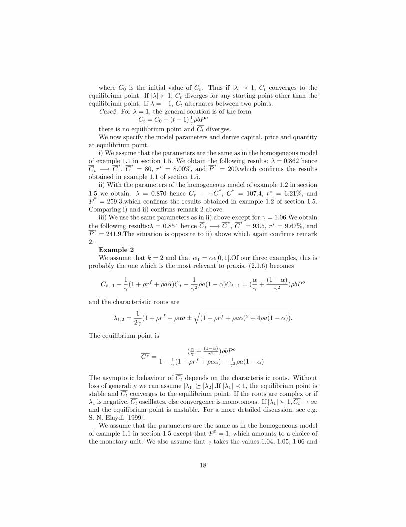
there is no equilibrium point and Ct diverges.We now specify the model parameters and derive capital, price and quantity

at equilibrium point.i) We assume that the parameters are the same as in the homogeneous model

of example 1.1 in section 1.5. We obtain the following results: � = 0:862 henceCt �! C

�; C

�= 80; r� = 8:00%; and P

�= 200;which con�rms the results

obtained in example 1.1 of section 1.5.ii) With the parameters of the homogeneous model of example 1.2 in section

1.5 we obtain: � = 0:870 hence Ct �! C�; C

�= 107:4; r� = 6:21%; and

P�= 259:3;which con�rms the results obtained in example 1.2 of section 1.5.

Comparing i) and ii) con�rms remark 2 above.iii) We use the same parameters as in ii) above except for = 1:06:We obtain

the following results:� = 0:854 hence Ct �! C�; C

�= 93:5; r� = 9:67%; and

P�= 241:9:The situation is opposite to ii) above which again con�rms remark

2.Example 2We assume that k = 2 and that �1 = ��[0; 1]:Of our three examples, this is

probably the one which is the most relevant to praxis. (2.1.6) becomes

Ct+1 �1

(1 + �rf + �a�)Ct �

1

2�a(1� �)Ct�1 = (

�

+(1� �) 2

)�bP o

and the characteristic roots are

�1;2 =1

2 (1 + �rf + ��a�

q(1 + �rf + �a�)2 + 4�a(1� �)).

The equilibrium point is

C� =(� +

(1��) 2 )�bP o

1� 1 (1 + �r

f + �a�)� 1 2 �a(1� �)

The asymptotic behaviour of Ct depends on the characteristic roots. Withoutloss of generality we can assume j�1j � j�2j :If j�1j � 1; the equilibrium point isstable and Ct converges to the equilibrium point. If the roots are complex or if�1 is negative, Ct oscillates, else convergence is monotonous. If j�1j � 1; Ct !1and the equilibrium point is unstable. For a more detailed discussion, see e.g.S. N. Elaydi [1999].We assume that the parameters are the same as in the homogeneous model

of example 1.1 in section 1.5 except that P 0 = 1; which amounts to a choice ofthe monetary unit. We also assume that takes the values 1:04; 1:05; 1:06 and

18

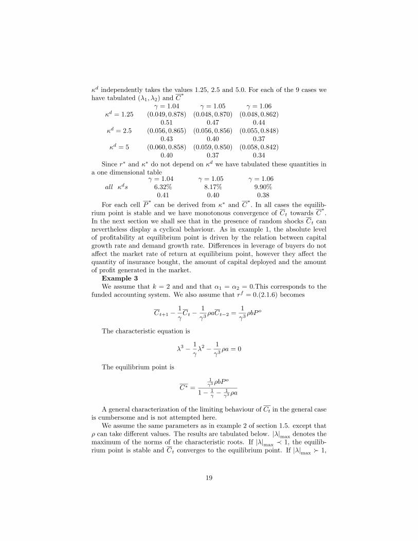
�d independently takes the values 1:25; 2:5 and 5:0: For each of the 9 cases wehave tabulated (�1; �2) and C

�

= 1:04 = 1:05 = 1:06�d = 1:25 (0:049; 0:878) (0:048; 0:870) (0:048; 0:862)

0:51 0:47 0:44�d = 2:5 (0:056; 0:865) (0:056; 0:856) (0:055; 0:848)

0:43 0:40 0:37�d = 5 (0:060; 0:858) (0:059; 0:850) (0:058; 0:842)

0:40 0:37 0:34

Since r� and �� do not depend on �d we have tabulated these quantities ina one dimensional table

= 1:04 = 1:05 = 1:06all �ds 6:32% 8:17% 9:90%

0:41 0:40 0:38

For each cell P�can be derived from �� and C

�: In all cases the equilib-

rium point is stable and we have monotonous convergence of Ct towards C�:

In the next section we shall see that in the presence of random shocks Ct cannevertheless display a cyclical behaviour. As in example 1, the absolute levelof pro�tability at equilibrium point is driven by the relation between capitalgrowth rate and demand growth rate. Di¤erences in leverage of buyers do nota¤ect the market rate of return at equilibrium point, however they a¤ect thequantity of insurance bought, the amount of capital deployed and the amountof pro�t generated in the market.Example 3We assume that k = 2 and and that �1 = �2 = 0:This corresponds to the

funded accounting system. We also assume that rf = 0:(2.1.6) becomes

Ct+1 �1

Ct �

1

3�aCt�2 =

1

3�bP o

The characteristic equation is

�3 � 1

�2 � 1

3�a = 0

The equilibrium point is

C� =

1 3 �bP

o

1� 1 �

1 3 �a

A general characterization of the limiting behaviour of Ct in the general caseis cumbersome and is not attempted here.We assume the same parameters as in example 2 of section 1.5. except that

� can take di¤erent values. The results are tabulated below. j�jmax denotes themaximum of the norms of the characteristic roots. If j�jmax � 1; the equilib-rium point is stable and Ct converges to the equilibrium point. If j�jmax � 1;

19

the equilibrium point is unstable and Ct diverges. If the characteristic equa-tion has dominating complex roots, the system oscillates. In addition to thesecharacteristics we have also recorded r�; C

�and P

�:

� 0:5 1 2 3 4j�jmax 0:82 0:70 0:85 0:96 1:04

oscillates no yes yes yes yesr� 10:48% 5:76% 3:03% 2:06% 1:56%

C�

90:6 109:4 122:1 127:0 129:6

P�

238:2 261:7 277:6 283:7 287:0From the above table we now know that the system of example 2 in section

1.5 converges for � = 3 and diverges for � = 4:From the above mentionedexample, however we also know that even the converging system displays strongoscillations around its equilibrium point during the �rst 30 periods. This is alsore�ected in the very high value of j�jmax. Based on this criteria, we see thateven the process with � = 2 shows signi�cant oscillations and only convergesslowly. In addition, the above systems are characterised by supply overcapacityand generate poor returns for values of � in excess of 1.Later we shall look at more sophisticated and more realistic ways to model

capital in�ows and out�ows. We shall see that capital �ows are often a con-tributing factor to underwriting cycles.

3 Selected Topics

In this section we consider di¤erent generalizations of the simpli�ed model whichare of practical relevance.

3.1 Stochastic Model

So far we have assumed that the pro�t stemming from business underwrittenin any given period is derived from the equilibrium between supply and de-mand and is deterministic. We now generalize the model to allow for random�uctuations around the expected value.There are di¤erent ways to take uncertainty into account within the frame-

work of our model. One can model underwriting year risk, �scal year risk or acombination thereof. We start with equation (2.1.5) which de�nes changes insurplus from one period to the next

Ct+1 = Ct + �rfCt + ��1�

mt + :::+ ��k�

mt�k+1:

We make the same model assumptions as in chapter 2. In addition we assumethat the pro�t contribution from each underwriting year in each �scal year issubject to random �uctuations. In the above formula, �l�

mt�l+1 is replaced

by �l�mt�l+1 +e�t�l+1;t (l = 1; :::k); where e�t�l+1;t is the random variable which

pertains to that part of the pro�t from underwriting year t� l+1 which emergesin �scal year t. The above formula becomes

Ct+1 = Ct + �rfCt + ��1�

mt + :::+ ��k�

mt�k+1 + �(e�t;t + :::+e�t�k+1;t):

20

The formula adequately re�ects insurance risk pertaining to new underwritingyears, i.e. underwriting years which contribute to the premium earned duringthe current �scal year. It does not take into account insurance risk stemmingfrom old underwriting years (loss development risk) nor does it take into account�nancial risk. A way to address the issue consists in introducing a furtherrandom variable e�t+1 which pertains to the �scal year and which re�ects thetwo above mentioned risk components. The formula becomes

Ct+1 = Ct+�rfCt+��1�

mt +:::+��k�

mt�k+1+�(e�t;t+:::+e�t�k+1;t)+e�t+1: (3.1.1)

Fiscal year risk is a generalization of the concept introduced in section 1.3.4.In addition to �nancial risk it also entails loss development risk.We make the following assumptions on the �rst and second order moments

of the above random variables.Assumptions1. E[e�s;t] = 0 all s; t; V ar[e�s;t] = ( s)2(�t�s+1)2�2� for 1 � t�s+1 � k;

Cov[e�s;t;e�u;v] = 0 for s 6= u or t 6= v

2. E[e�t] = 0 all t; V ar[e�t] = ( t)2�2�; Cov[e�s;e�t] = 0 for s 6= t

3. Cov[e�s;t;e�u] = 0 for all s; t; u:The �rst assumption ensures that random �uctuations stemming from un-

derwriting year risk are bias free. The standard deviation of random �uctuationsis proportional to a scale factor depending on the underwriting year ( s) andto a factor depending on the earning period (�t�s+1):Random �uctuations per-taining to di¤erent underwriting periods are uncorrelated. Random �uctuationspertaining to pro�ts emerging in di¤erent �scal years are also uncorrelated. Thesecond assumption makes similar statements on random �uctuations stemmingfrom �scal year risk. Finally we assume that underwriting year risk and �scalyear risk are uncorrelated.Remarks1. If �� = �� = 0; (3.1.1) becomes a simple di¤erence equation. This is the

di¤erence equation corresponding to our stochastic process.2. Let e�t = e�t;t +e�t;t+1 + :::+e�t;t+k�1 denote the risk pertaining to under-

writing year t. Because of assumption 1 we haveV ar[ e�t] = ( t)2�2�(�21 + �22 + :::+ �2k):TheoremWithin the framework of the so de�ned model, the standardized centered

process�Ct � �

is an autoregressive process of order k. The mean � of the

autoregressive process is equal to the equilibrium point of the correspondingdi¤erence equation.ProofUsing (2.1.4a), re-arranging terms and dividing each term by t+1 we obtainCt+1 � 1

(1 + �rf + �a�1)Ct � 1

2 �a�2Ct�1 � :::�1 k�a�kCt�k+1 �

�(�1 +�2 2 + :::+

�k k)�bP o = �

t+1 (e�t;t + :::+e�t�k+1;t) + e�t+1 t+1

We de�nenC�t

o=�Ct � �

as the deviation process of

�Ctfrom its mean

21

�. We introduce the following notation

e�t+1 = �

t+1(e�t;t + :::+e�t�k+1;t) + e�t+1

t+1

Inserting Ct = C�t + � in the above equation we obtain

C�t+1 � 1

(1 + �rf + �a�1)C

�t � 1

2 �a�2C�t�1 � :::� 1

k�a�kCt�k+1+

+�� 1 (1 + �r

f + �a�1)�� 1 2 �a�2�� :::�

1 k�a�k�

�(�1 +�2 2 + :::+

�k k)�bP o = �t+1

The mean � is de�ned by the fact that all terms on the left hand side of theequation which do not contain C

�t must add up to 0. Hence

� =(�1 + :::+

�k k)�b

(1� 1 �

1 �r

f )� (�1 + :::+�k k)�a

P 0

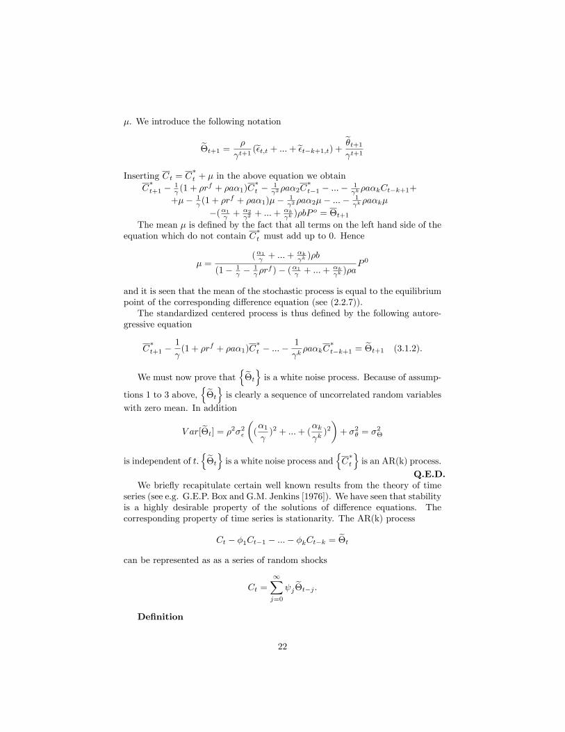
and it is seen that the mean of the stochastic process is equal to the equilibriumpoint of the corresponding di¤erence equation (see (2.2.7)).The standardized centered process is thus de�ned by the following autore-

gressive equation

C�t+1 �

1

(1 + �rf + �a�1)C

�t � :::�

1

k�a�kC

�t�k+1 = e�t+1 (3.1.2).

We must now prove thatne�to is a white noise process. Because of assump-

tions 1 to 3 above,ne�to is clearly a sequence of uncorrelated random variables

with zero mean. In addition

V ar[e�t] = �2�2�

�(�1 )2 + :::+ (

�k k)2�+ �2� = �2�

is independent of t:ne�to is a white noise process and nC�to is an AR(k) process.

Q.E.D.We brie�y recapitulate certain well known results from the theory of time

series (see e.g. G.E.P. Box and G.M. Jenkins [1976]). We have seen that stabilityis a highly desirable property of the solutions of di¤erence equations. Thecorresponding property of time series is stationarity. The AR(k) process

Ct � �1Ct�1 � :::� �kCt�k = e�tcan be represented as as a series of random shocks

Ct =1Xj=0

j e�t�j :De�nition

22

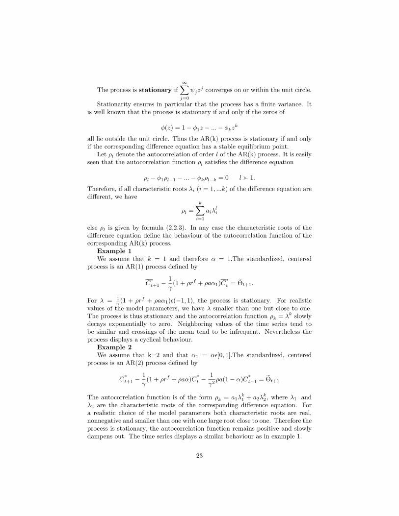
The process is stationary if1Xj=0

jzj converges on or within the unit circle.

Stationarity ensures in particular that the process has a �nite variance. Itis well known that the process is stationary if and only if the zeros of

�(z) = 1� �1z � :::� �kzk

all lie outside the unit circle. Thus the AR(k) process is stationary if and onlyif the corresponding di¤erence equation has a stable equilibrium point.Let �l denote the autocorrelation of order l of the AR(k) process. It is easily

seen that the autocorrelation function �l satis�es the di¤erence equation

�l � �1�l�1 � :::� �k�l�k = 0 l � 1:Therefore, if all characteristic roots �i (i = 1; :::k) of the di¤erence equation aredi¤erent, we have

�l =kXi=1

ai�li

else �l is given by formula (2.2.3). In any case the characteristic roots of thedi¤erence equation de�ne the behaviour of the autocorrelation function of thecorresponding AR(k) process.Example 1We assume that k = 1 and therefore � = 1:The standardized, centered

process is an AR(1) process de�ned by

C�t+1 �

1

(1 + �rf + �a�1)C

�t = e�t+1:

For � = 1 (1 + �rf + �a�1)�(�1; 1); the process is stationary. For realistic

values of the model parameters, we have � smaller than one but close to one.The process is thus stationary and the autocorrelation function �k = �k slowlydecays exponentially to zero. Neighboring values of the time series tend tobe similar and crossings of the mean tend to be infrequent. Nevertheless theprocess displays a cyclical behaviour.Example 2We assume that k=2 and that �1 = ��[0; 1]:The standardized, centered

process is an AR(2) process de�ned by

C�t+1 �

1

(1 + �rf + �a�)C

�t �

1

2�a(1� �)C�t�1 = e�t+1

The autocorrelation function is of the form �k = a1�k1 + a2�

k2 , where �1 and

�2 are the characteristic roots of the corresponding di¤erence equation. Fora realistic choice of the model parameters both characteristic roots are real,nonnegative and smaller than one with one large root close to one. Therefore theprocess is stationary, the autocorrelation function remains positive and slowlydampens out. The time series displays a similar behaviour as in example 1.

23

For an in depth discussion of the characteristics of AR(2) processes as wellas for speci�c examples see e.g. G.E.P. Box and G.M. Jenkins [1976].

3.2 Open Markets

So far we have assumed that the change in capital on the supply side of themarket stems exclusively from retained earnings or losses. In practice manyinsurance markets experience signi�cant capital in�ows and out�ows. These aredriven by the perceived pro�tability of the respective markets. Investors usuallybase their assessment of the future pro�tability of a market on its historicalpro�tability. One or many very pro�table years lead to an in�ow of capital. Aseries of highly unpro�table years drives capital out of the market.The barriers to entry vary from market to market. Markets where the dis-

tribution is dominated by tied agents or by employees of insurance companieshave high barriers to entry. It is the case of many continental European per-sonal lines markets. Markets where the distribution is dominated by brokershave low barriers to entry. This applies e.g. to the UK market. Wholesalebroker markets have the lowest barriers to entry. The international reinsuranceis a case in point.Barriers to exit are generally higher than barriers to entry. The main reasons

are regulatory constraints. One should however not forget that many insurancegroups are active in di¤erent market segments and can shift capital from onemarket segment to another without taking capital out of any legal entity.The lag between the time when pro�table business is written and the entry

of new capital can be signi�cant. Depending on the accounting system theremay be a lag between the time when business is written and the time whenthe corresponding results emerge. Pro�ts earned during any given �scal yearonly become apparent to new investors during the following calendar year asthe pro�t and loss accounts are made public. Setting up new insurance entitiestakes time.Only extraordinary pro�ts or losses trigger a capital �ow. As a consequence

the capital change at the end of a �scal year is usually not a linear function ofthe pro�t or loss in that �scal year or in previous �scal years.We propose a simple model which takes into account the features mentioned

above. We assume that premium underwritten in year t is fully earned duringthe same year. We assume that capital in�ows and out�ows take place with alag of one year. The di¤erence equation de�ning the change in equity from oneyear to the next is

Ct+1 = Ct+�rfCt+��

mt +�+(�

mt�1�

rs+�sPmt�1)

++��(�mt�1�

rs��sPmt�1)

� (3.2.1)

Where we have used the following notationx+ = x if x � 0 else x+ = 0x� = x if x � 0 else x� = 0�+ and �� are two non-negative parameters to be speci�ed later.

24

rs+ and rs� are the threshold returns above (respectively below) which capital

�ows into (respectively out of) the market. It is reasonable to assume rs+ � rs �rs� which we shall do from now on.The model stipulates that any excess pro�t triggers a capital in�ow which is

equal to a multiple �+ of the actual excess pro�t. Any inadequate pro�t triggersa capital out�ow which is equal to a multiple �� of the amount by which therequired minimum pro�t has been missed. The model is de�ned by a piecewiselinear di¤erence equation with constant coe¢ cients.In the special case where rs+ = rs� = rs and �+ = �� = � we have

Ct+1 = Ct + �rfCt + ��

mt + �(�

mt�1 �

rs

�sPmt�1) (3.2.2)

The model assumptions of chapter 2 remain valid. Using the representation of�mt given by (2.1.4a) as well as a similar representation for P

mt which we obtain

from (2.1.3)

Pmt = eCt+f tP 0 with e =

�d�s

�s + �d + �s�d( rs

�s �rd

�d)and f =

�s

�s + �d + �s�d( rs

�s �rd

�d)

we obtain the following di¤erence equation for the standardized capitalCt+1 =

1 (Ct + �r

fCt + �aCt + �bP0) + 1

2 �+((a�rs+�s e)Ct�1 + (b�

rs+�s f)P

0)++

+ 1 2 ��((a�

rs��s e)Ct�1 + (b�

rs��s f)P

0)� (3:2:3)

We make the following case distinctionCase 1

For Ct�1 � b�rs+�s f

�a+rs+�s e

P 0 =�s+�s(rs�rs+)

�s+�d(rs+�rd�s

�d)P 0

�s

(3.2.3) becomes

Ct+1 �1

(1 + �rf + �a)Ct �

�+ 2(a�

rs+�se)Ct�1 =

1

�bP 0 +

�+ 2(b�

rs+�sf)P 0

The equilibrium point C�1 and the characteristic roots �1;�2 of the di¤erence

equation are derived in the usual way. Hence

�1;2 =1

2 ((1 + �rf + �a)�

r(1 + �rf + �a)2 � 4�+(�a+

e

�srs+)

which leads to the following re�nement of the case distinctioni) For �+ � 1

4(1+�rf+�a)2

�a+ e�s r

s+both characteristic roots are real, positive and

smaller than 1: Ct converges monotonously towards C�1:If C

�1 is in domain 1

(i.e. the domain de�ned by case 1) or on the boundary of domain 1, C�1 it is an

equilibrium point. Else Ct jumps into domain 2 or 3 after a certain number ofsteps.ii) For 1

4(1+�rf+�a)2

�a+ e�s r

s+

� �+ � 2

�a+ e�s r

s+

the characteristic roots are

conjugate complex numbers with norm smaller than 1: Ct converges towards

25

C�1. Convergence is cyclical, therefore Ct may jump into domain 2 or 3 after a

certain number of steps.iii) For �+ � 2

�a+ e�s r

s+the characteristic roots are conjugate complex

numbers with norm larger than 1: Ct is cyclical and diverges. After a certainnumber of steps, Ct jumps into domain 2 or 3.Case 2For

�s+�s(rs�rs+)�s+�d(rs+�rd

�s

�d)P 0

�s � Ct ��s+�s(rs�rs�)

�s+�d(rs��rd�s

�d)P 0

�s

(3.2.3) becomes

Ct+1 �1

(1 + �rf + �a)Ct =

1

�bP 0

The characteristic root is

� =1

(1 + �rf + �a)

For a realistic choice of model parameters we have ��(0; 1): Ct converges

towards C�2 =

1 �b

1� 1 �

1 �r

f� � a

P 0:If C�2 is in domain 2, it is an equilibrium point

and domain 2 is absorbing.Case 3For

�s+�s(rs�rs�)�s+�d(rs��rd

�s

�d)P 0

�s � Ct�1

(3.2.3) becomes

Ct+1 �1

(1 + �rf + �a)Ct �

�� 2(a�

rs��se)Ct�1 =

1

�bP 0 +

�� 2(b�

rs��sf)P 0

The �ner case distinction is similar to case 1 above and is omitted here.Numerical ExampleWe assume the same parameters as for the homogeneous model of example

1.1 of section 1.5 except that we do not specify P 0 but use the parameter todenote the monetary unit. In addition we assume that rs+ = rs = 0:08 andrs� = 0:We shall consider the implications of di¤erent choices for �+ and ��:The di¤erent domains are de�ned as follows

Domain 1: Ct�1 � 0:4P 0Domain 2: 0:4P 0 � Ct�1 � 0:552P 0Domain 3: 0:552P 0 � Ct�1:

C�1 = 0:4P

0 irrespective of the value of �+:C�2 = 0:4P

0:Thus C�1 = C

�2 = C

�

is an equilibrium point both for domain 1 and 2. C�3�[0:4P

0 ; 0:552P 0) for���[0;1): Thus C

�3 is not an equilibrium point for domain 3.

Domain 1: for �+ � 0:819; Ct converges monotonously towards C�:For

0:819 � �+ � 4:41; Ct converges towards C�. Convergence is cyclical, therefore

Ct may jump into domain 2 or 3 after a certain number of steps. For 4:41 � �+;Ct is cyclical and diverges. After a certain number of steps, Ct jumps intodomain 2 or 3.

26

Domain 3: the corresponding thresholds for �� are 0:975 and 5:25: Howeverirrespectively of the choice of ��, Ct will move out of domain 3, either throughmonotonous or cyclical convergence towards C

�3; which is inside domain 2, or

because Ct diverges.From the above analysis we see that for �+ � 4:41 and �� � 5:25; Ct

eventually converges to C�irrespectively of the starting values C0 and C1:

However Ct may display strong oscillations. We have computed an examplewith �+ = �� = 4 and C0 = C1 = 0:3P

0: We have obtained C2 = 0:40P 0 andC3 = 0:49P 0: After this signi�cant initial overshooting, the process convergesmonotonously to C

�= 0:40P 0:

For �+ � 4:41 and �� � 5:25 no general statement can be made. Theprocess can converge to the equilibrium point after signi�cant �uctuations or itcan diverge by oscillating between domain 2 and 3.The technique we have used to analyze the model can in principle be applied

to any piecewise linear model with constant coe¢ cients.RemarkThe special case (3.2.2) above, leads to a more straightforward solution. The

di¤erence equation is

Ct+1 �1

(1 + �rf + �a)Ct �

�

2(a� rs

�se)Ct�1 =

1

�bP 0 +

�

2(b� rs

�sf)P 0

and the characteristic roots are

�1;2 =1

2 ((1 + �rf + �a)�

r(1 + �rf + �a)2 � 4�(�a+ e

�srs):

Because typically � � 1, �1and �2 are likely to be complex or even to belarger than one in norm. Hence the solutions are cyclical or even unstable.Open market models are much more prone to cycles than markets which do notexperience capital in- and out�ows. This is con�rmed by the fact that marketswith low barriers to entry tend to experience strong underwriting cycles.With rs+ = rs� = 0:08 and with the other parameters as above, The solution

of the di¤erence equation is a dampened sine wave for 4:41 � �+ = �� � 0:819and diverges for �+ = �� � 4:41:

3.3 Random Shocks

Let us assume that we want to model the impact of a stress scenario on an in-surance market. As an example we assume that the assets overperform duringa period of �ve years leading to a 4% net (after tax and dividends) extraordi-nary increase in capital p.a. At the end of the period, the overperformance iscorrected at once and the capital su¤ers a drop of 17.8%. In addition a furtherdrop of 7.5% of the remaining capital occurs as a consequence of market widesigni�cant adverse loss developments. This scenario is close to what happenedin the late 1990s and early 2000s. After a protracted period of very favorablestock market performance, a dramatic correction occurred in 2001 and 2002.

27

It was accompanied by signi�cant adverse loss developments in respect of USbusiness underwritten in the late 1990s. It is estimated that on a worldwidebasis, the amount of equity deployed to underwrite insurance risks dropped byapproximately 25%.One possibility to model such risks is to use the stochastic model of section

3.1 and to make the appropriate assumptions on the distribution of e�t: A betterinsight can be gained by generalizing the simpli�ed model of chapter 2 throughthe introduction of a deterministic correction factor. We therefore assume thatthe di¤erence equation de�ning the change in surplus from one period to thenext is

Ct+1 �1

(1 + �rf + �a+ �t)Ct =

1

�bP o

�t is the correction factor. Note that the di¤erence equation has now timedependent parameters. The market rate of return during a given period isde�ned by the standardized version of (2.1.1).We have used the parameters of the homogeneous version of model 1.1 in

section 1.5 except that we have set P 0 = 1 and C0 = 0:4: To re�ect the above de-scribed scenario, we have assumed (�1;:::�5;�6;�7;:::) = (0:04; :::0:04;�0:24; 0; :::):Wehave obtained the following results

t Ct [MU] rmt [%] Pmt [MU]0 0:400 8:00 1:005 0:462 4:38 1:086 0:348 11:47 0:9410 0:371 9:86 0:9615 0:386 8:87 0:9820 0:394 8:41 0:99It is seen that during the �rst phase, capital grows too quickly leading to an

oversupply of capacity and depressing the market rate of return. After year �vea correction takes place, capital is destroyed, the market rate of return soars andthe amount of insurance bought declines. Over time the system slowly comesback to normal.It is realistic to assume that the extraordinary returns achieved during year

six and the immediately following years trigger an in�ow of capital into themarket. We have therefore considered a combination of this example and theexample of section 3.2. The process also converges back to normal but it doesso after overshooting with a relative maximum of capital reached in year nine.The larger �+; the more severe the overshooting. This is an example of anunderwriting cycle reinforced by the interaction of di¤erent factors.

3.4 Summary and Conclusions

From the models proposed and from the di¤erent examples, we can draw thefollowing conclusions:The equilibrium market rate of return is driven by the target rate of return

of suppliers and by the balance of demand growth and targeted capital growth.

28

At equilibrium point, the parameters characterizing the buyers (rd; �d; �d) havean in�uence on the quantity of insurance being transacted but not on its price.Cycles are induced by the supply side. Pro�ts and losses feed back into

surplus leading to shifts in supply which o¤set the pro�t or loss trend. Capitalin�ows and out�ows triggered by extraordinary pro�ts and losses induce under-writing cycles. These supply induced cycles are exacerbated by reporting lagsstemming from accounting or regulatory factors. Random shocks (e.g. adverseloss developments or catastrophes) create �uctuations in results and can inducecycles through a depletion of the capital of insurance companies. The changes-in-expectations hypothesis mentioned in section 1.2 can be viewed as a shift insuppliers�leverage.Cycles are induced by the demand side. A temporary acceleration or de-

celeration of demand growth leads to �uctuations in the rate of return. Demandshifts, such as sudden decreases in base demand can also trigger �uctuations inreturns. They usually occur as a reaction to a dramatic contraction in supply.Cycles are induced by external factors. Signi�cant changes in the value

of assets can lead to underwriting cycles because they have an impact on theamount of capital available to insurance companies. Changes in interest rateshave no direct impact on insurance returns. They lead to changes in the facevalue of insurance premiums but have no direct in�uence on insurance price orquantity.The above factors seldom act in isolation but interact with each other, thus

possibly exacerbating �uctuations in results and creating underwriting cycles.The simpli�ed model and its generalizations enable a simultaneous evaluationof the impact of di¤erent factors. The in�uence of each factor can be quanti�edby analyzing the solutions of di¤erence equations.The stochastic version of example 2 leads to an AR(2) processes for the

capital, the pro�t and the pure risk premium. This is in line with the �ndingsof the di¤erent articles which have �tted time series to real life data.LiteratureLawrence A. Berger, A Model of the Underwriting Cycle in the Property/Liability

Insurance Industry, The Journal of Risk and Insurance, Vol. LV, No. 2, 1988.George E. P. Box and Gwilym M. Jenkins, Time Series Analysis, Holden-

Day, 1976.J. David Cummins and J. F. Outreville, An International Analysis of Un-

derwriting Cycles in Property-Liability Insurance, The Journal of Risk and In-surance, Vol. LIV, No. 2, 1987.Neil A. Doherty and Han Bin Khang, Interest Rates and Insurance Price

Cycles. Journal of Banking and Finance, 12, 1988.Saber N. Elaydi, An Introduction to Di¤erence Equations, Springer, 1999.Martin F. Grace and Robert E. Hoyt, External Impacts on the Property-

Liability Insurance Cycle, The Journal of Risk and Insurance, Vol. 62, No. 4,1995.Gene Lai and Robert C. Witt, Changed Insurers Expectations: An Insurance-

Economics View of the Commercial Liability Insurance Crisis. Journal of In-surance Regulation, 10. 1992.

29

Gene Lai, Robert C. Witt, Hung-Gay Fung, Richard D. McMinn and PatrickL. Brockett, Great (and not so Great) Expectations: An Endogeneous EconomicExplication of Insurance Cycles and Liability Crises. The Journal of Risk andInsurance, Vol. 67, No. 4, 2000.Joan Lamm-Tennant and Mary A. Weiss, International Insurance Cycles:

Rational Expectations/Institutional Intervention, The Journal of Risk and In-surance, Vol. 64, No. 3, 1997.René Schnieper, Portfolio Optimization, ASTIN Bulletin, Vol. 30, No. 1,

2000.Emilio C. Venezian, Ratemaking Methods and Pro�t Cycles in Property and

Liability Insurance, The Journal of Risk and Insurance, Vol. LII, No.3, 1985.Mary A. Weiss and Joon-Hai Chung, U.S. Reinsurance Prices, Financial

Quality and Global Capacity. The Journal of Risk and Insurance, Vol. 71, No.3, 2004.Ralph Winter, The Liability Crisis and the Dynamics of Competitive Insur-

ance Markets. Yale Journal on Regulation 5, 1988.

30