MODELLING REGULATORY DISTORTIONS WITH REAL OPTIONS: AN EXTENSION* JAMES ALLEMAN

University of Colorado – Boulder & Columbia University PAUL RAPPOPORT

Temple University & Columbia University Hirofumi Suto

NTT East, Tokyo, Japan

ABSTRACT

The introduction of uncertainty can make a significant difference in the valuation of a project. In a regulatory envirormwent, this manifests itself, inter alia, in situations where regulatory constraints can affect the valuations of a firm’s investment which, in turn, has an adverse impact on consumers’ welfare. In particular, the inability of a regulated firm to exercise any or all of the delay, abandon, start/stop, and time-to-build options has an economic and social cost. With this view in mind, we specify and estimate a model where regulatory delay constraints impact the firm’s cash flow and its investment valuation with real options methods. This paper uses real options analysis to address issues of regulation that have not been adequately quantified. We show that regulatory constraints on cash flow have an impact on investment valuations. Specifically, a model is developed to estimate the cost of regulation by constraining the delay option. We show that the cash flow constraints and the inability to delay has a significant cost. Because some costs are not recognized in a static view of the world, this failure to recognize the operation and implications of non-flexibility by regulators (which can be modelled by real options methods) will lead to a reduction in company valuations which in turn will lead to a reduction in economics welfare. The impact of regulation changes the variance used in the real options model. For example, the price cap or discounted access charges or other regulatory devices dampen the possibility of a high return contract, thus affecting the variance of returns. We model the regulatory constraint by constraining variance, σ2, in the option model. As intuition would suggest, as the constraint becomes tighter, the probability that the deferred option will pay-off is diminished.

Preliminary Draft, not for citation or quotation Keywords: Real Options, Decision, Investment, Economic Methodology; Statistical Decision Theory, Criteria for Decision-Making under Risk and Uncertainty, Regulatory Distortions JEL Classification: B41, C44, D81, G13

* This paper draws on and expands works by the authors – Alleman & Rappoport (2002) and Alleman, Suto, & Rappoport (2004). The authors would like to thank Larry Darby, Alain deFontenay, Gary Madden, Eli Noam, Michael Noll, Scott Savage, and Chris Schlegel for useful comments and discussion of the ideas developed in this paper. Of course, the usual disclaimer applies.

2

INTRODUCTION1 The real options pricing approach utilizes financial option principles to value real assets under uncertainty. In this paper, we evaluate regulatory actions ex post in order to determine the impact of regulatory constraints on investment decsion-making. The genesis of this research began when one of the authors evaluated telecommunications cost models whose foundation was based on the applications of traditional discounted cash flow analysis – exactly the method that real options methodology has shown can give terribly wrong results (Alleman 2002a). For example, if regulation does not account for management’s flexibility to respond to constraints that regulation imposes on the regulated firm, we show that the frim may make inefficient management and finacial decsions.from society’s perspective Regulation leads to constraints on prices or on profits. Regulation also surfaces in the context of the obligation to serve. Under the current practice in most countries, whenever a customer demands service, the incumbent carriers are obligated to provide the service. It is part of the common carrier obligation. Under the obligation to serve requirement, if the customer proves unprofitable, the carrier still must nevertheless serve this customer. This is in contrast to discretionary services offered by the telephone company providers, such as digital subscriber line (DSL), where reports of consumers’ complaints about the unavailability or the slow rollout of the service are heard. Consider broadband service. If the telephone company chooses to limit the availability of broadband service, this is an example of a delay option. If the telephone company wants to cease providing payphone service, we have an example of the abandonment option. Alternatively, if the company faces a common carrier obligation to provide broadband services and to maintain payphones, the requirement to provide broadband services eliminates the company’s option to delay. Similarly, the inability to exit the payphone business eliminates the firm’s ability to exercise its abandonment option. In the delay case, concerns with the “digital divide” have prompted proposed legislation in the United States to mandate the increased deployment of broadband services. If passed, this action would limit the companies’ ability to delay. In the second case, with the rapid increase in mobile telephone usage, payphone service has experienced a serious decline in its revenues. When the phone companies attempt to exit the service, the regulators forbid it.2 In the dynamic world, demand, technology, factor prices and many other parameters of interest to a company are subject to uncertainty. The principal uncertainty is the demand for goods, which, in turn, impacts cash flow, investment valuations, profits, and economic depreciation among other economic variables. We construct a model where, using an investment model incorporating the real option method. With the continuous-additive model in an uncertain world we show the cost of the regulatory constraint. We illustrate this approach with a stylized binomial model. This model provides an intuitive

1 This section is adapted from Alleman and Rappoport (2002). 2 This is true in the United States and Japan. The authors have not investigated it in other countries.

3

understanding of the result that regulation has a cost, thus showing that regulation can restrict the flexibility of the firm through the imposition of price constraints, or by imposing costs associated with delay, abandonment, or shutdown/restart options. Since the cost models used for public policy decision makers do not account for the time-to-build options available to the firm, if these regulatory impacts are left unaccounted for, there are significant costs to the firm and to society. (One of the clearest examples of the telecommunications regulators’ failures to apply dynamic analysis is in the use of cost models and a type of long run incremental cost methodology to determine prices and obligations-to-serve subsidies (Alleman 1999)).

PREVIOUS RESEARCH

Regulatory Research The literature is divided into three areas: first, regulation’s impact on investment – either rate-of-return or incentive regulation – usually in a static context though occasionally with dynamic models of investment behavior; second, generic real options analysis; and third, real options applied to telecommunications. The first two areas have been adequately reviewed elsewhere. For a review of telecommunications regulation prior to the late-eightys, see Kahn (1988); a review of the current state-of-the-art in telecommunications is found in Laffont and Tirole (1999). The static and dynamic aspects of investment under various forms of regulation and optimal (Ramsey) pricing may be found in Biglaiser and Riordan (2000). Most of this literature assumes static models of which the Averch-Johnson is the most well know (Averch 1962). These models show rate-of-return regulation does not provide the incentive for the firm to minimize costs or capital investments. If the firm’s growth is handled at all, it is through exponential models with time as the explanatory variable. Economic depreciation is treated exogenously. The dynamic models are deterministic, complete information growth models.

Real Options Research The literature on real-options research from the financial perspective is reviewed and integrated in Trigeorgis (1996), and from the economists’ perspective covered extensively in Dixit and Pindyck (1994) or, for a briefer account, in their 1995 article (Dixit 1995). Dixit and Pindyck and other economist’s usually only look at the delay option. The finance literature is fuller in its coverage of the various aspects of all of the options available to a firm, for example Hull (2000) has an extensive coverage of options, as does Luenberger (1998). See Smith and Nau (1995) for the relationship between decision trees and real options.

Real Options Applied to Telecommunications A limited, but growing, literature exists in the applications of real options to telecommunications. Hausman has applied the real options methodology to examine the sunk cost of assets and the delay option in the context of unbundled network elements (UNEs) (1999 and 2003). Ergas and Small (2000) have applied the real options methodology to examine the sunk cost of assets and the regulator’s impact on the distribution of returns (2000). They establish linkages between regulation, the value of the

4

delay option and economic depreciation. Small (1998) studied investment under uncertain future demand and costs with the real options method. More recently, d’Halluin, et al. (2004a) have applied real options methodology to an ex post analysis of capacity in long distance data service. The same authors also applied the methodology to the wireless service issues (2004b). Hori and Mizuno (2004) have applied real options to access charges in the telecommunications industry; Pak and Keppo (2004) have applied the approach to network optimization; and Kulatilaka and Lin apply the methodology to strategic investment in technology standards (2004).

REAL OPTIONS

What are real options? A financial option is the right to buy (a call) or sell (a put) a stock, but not the obligation, at a given price within a certain period of time. If the option is not exercised, the only loss is the price of the option, but the upside potential is large. The asymmetry of the option, the protection from the downside risk with the possibility of a large upside gain, is what gives the option value. With real options analysis, the idea is similar. The manager identifies options within a project and their exercise prices. If the future is good, the option is exercised; if the outlook is uncertain or bad, the option is not exercised. If the option is not exercised the only loss is the price of the option. The real options analysis provides a means of capturing the flexibility of management to address uncertainties as they are resolved. The flexibility that management has includes options to defer, abandon, shutdown/restart, expand, contract, and switch use (see TABLE 1). This methodology forces the firm to assess its simple view of valuation to one that more closely matches the manner in which the firm operates. The use of real options lets the firm modify its actions after the state-of-nature has revealed itself. For example, if demand fails to meet expectations, the firm may chose to delay investment rather than proceed along their original business case. The deferral option is the one that is generally illustrated and is treated as analogous to a call option. But real options analysis can be applied to evaluation of other management alternatives, for example shutdown and restart, time-to-build, or extend the life of a project or enterprise.

TABLE 1: Description of Options Option Description

Defer To wait to determine if a “good” state-of-nature obtains Abandon To obtain salvage value or opportunity cost of the asset Shutdown & restart To wait for a “good” state-of-nature and re-enter Time-to-build To delay or default on project – a compound option Contract To reduce operations if state-of-nature is worse than expected Switch To use alternative technologies depending on input prices Expand To expand if state-of-nature is better than expected Growth To take advantage of future, interrelated opportunities

ANALYSIS

5

Assumptions and Model

To explain the application of real options to model regulatory distortions, the following stylized assumptions are made. Cash flows shifts each period based on a probability – the cash flow is high (a good result) with probability of q or low (a bad result) with probability of (1–q). The model is for two periods and the intertemporal cross-elasticities of demand are assumed to be zero. These simplifying assumptions are enough to capture the effects of time and uncertainty; it leads to an easy understanding of the methodology; and serves as a foundation of the more complex analysis. We explore only one facet of this simple, but not unrealistic assumption, that cash flows are uncertain. We will explore the role of management’s flexibility in dealing with two uncertainties when management is constrained in its behavior by regulation: first by the obligations to serve and then with a regulatory constrain on prices. We contrast this with management’s unconstrained actions. (This analysis is applicable only when the firm has freedom from other regulatory constraints, such as quality of service constraints. While this will not change the nature of the results, it may well change the magnitude of the options.) Under the traditional engineering-economics methodology, the value of the investment would be evaluated with an expected value of the discounted present value of the profit function. This requires, inter alia, the determination of the “correct” discount rate. To account for uncertainty the rate is adjusted for risk, generally using the capital asset pricing model (CAPM). In the regulatory context, this would be equivalent to the determination of the rate-of-return for the firm. In the rate base, rate-of-return regulation context, a “historical” year is chosen and the rate-of-return determined. Prospective costs and revenues are assumed to be estimated with the past and the historical year, representing the mean of that past. Before competition entered the telecommunications industry, discounted present value techniques were a useful analytical technique. The industry had stable, predictable revenues and cost, and hence, cash flow; but more recently, the industry has become volatile (Noam 2002) and (Alleman 2002b). Our analysis differs from this present value approach in that it treats the investment and cash flow prospectively as a model in which an investment has two possible outcomes: a good result or a bad result. A simple binomial real option model can analyze the investment.3 Viewed in this fashion, the question is: what is the investment worth with and without management flexibility? In addition to the cash flow constraint, we explore condition to delay in detail. Earlier we noted other conditions in which regulation can have impact on valuations: abandonment, shutdown/restart and time-to-build options.

3. The simplicity of the model should not mis-lead the reader. The two period models can be expanded into an n-period model. Cox, Ross, and Rubinstein (1979) show how to solve these models and how, in the limit, the results converge to the Black-Scholes option pricing result.

6

REGULATORY DISTORTION

The economist is concerned with the social welfare. The nominal purpose of regulation is to optimize social welfare and ensure that monopoly rents are eliminated from the firm’s prices. This requires knowledge of economics cost and benefits. Generally benefits are measures by the consumers’ surplus; economics cost are estimated by the firm’s historical accounting costs. Both can be difficult to measure, but what we argue here is that not recognizing some costs, i.e., not knowing what to measure, means that the social welfare is distorted. The interaction of the regulation with valuation bears on welfare in several dimensions. First, unrecognized costs on the part of the regulator community means that the prices set by it will not be correct. Second, if the financial community recognizes that the regulatory is not accounting for all the costs of the enterprise, then it will be more expensive to raise debt and equity capital, which, in turn, will increase the cost in a vicious cycle, raising the cost to the consumers. A major cost that has not been adequately identified or quantified is the obligation to serve. Under the current practice in most countries, whenever a customer demands service, the incumbent carriers are obligated to provide the service. It is part of the common carrier obligation. The United States Congress has had legislation before it that would mandate that the telephone companies provide mandatory broadband service. This would not allow the firms to assess the market, determine the best time to enter and where best to enter. They would be on a specific time and geographic schedule. The firms have lost the option to delay. Moreover, if the customer proves unprofitable, the carrier still must retain this customer. Thus, they also lose their right or option to abandon the service. (The argument that the expansion of the network provides an external benefit – an externality – beyond the value of an additional subscriber may be an offset to this cost, but the externality argument is not compelling in the United States or any area that has significant penetration of telephone service, see Crandall and Waverman (1999).)

In the broadband situation, the incumbent carriers are precluded from exercising the option to delay. A related option is the ability to shutdown and restart operations. This, too, is precluded under the regulatory franchise. Finally, the time-to-build option, which includes the ability to default in the middle of a project, would not be available in the current regulatory context. The lack of options has not been considered in the various cost models that have been utilized by the regulatory community for a variety of policy purposes. Clearly, the lack of these options imposes a cost to the firm and to society.4 In a previous paper (Alleman & Rapport 2002), we used the deployment of DSL to illustrate the delay option, and then the learning option. We indicate how both may be quantified and suggest the parameters which are relevant for these options. In this paper we draw from work

4 This is not to imply that these public policies be abandon, but in order to weigh the policy alternatives, their costs must be understood.

7

which simplifies the investment criterion using real options methodology to evaluate the delay option (Alleman, Rappoport, & Suto 2003). How can options be valued? Black and Scholes examined a method nearly 30 years ago for pricing financial options, and it's been much refined since then. See, for example (Nembhard 2000), for various methods and techniques to solve these real options problems. The technique can also be applied to physical or real assets. To understand the intuition of the method, consider the stock-option comparison. Three things influence the price of stock options: the spread between the current and the exercise price, the length of time for which the option is good, and the volatility of the stock in question. The current price of the asset is known, and the exercise price at which the stock can be purchased sometime in the future is set. The greater the difference between the two, the lower the options price because only a great change in the market will make the stock's value climb above the exercise price and pay off for the owner. And big shifts are less likely than small ones. The date at which the option expires also is a factor. The longer the option lasts, the greater the chance that the stock will become higher (“in-the-money”) and go beyond the exercise price, and that the owner will make a profit. So, the price is higher. Finally, the volatility of the stock price over time influences the option price. The greater the volatility, the higher the price of the option, because it's more likely the price will move above the exercise price and the owner will be in-the-money. Black and Scholes consider these factors to solve the problem of pricing the option. One important attribute of real options as opposed to the traditional discounted cash-flow analysis is the treatment of uncertainty. In discounted cash-flow analysis, increased risk is handled by increasing the discount rate; the more risk, the higher the return the company has to earn as a reward for investing. This has the effect of decreasing the value of the cash flow in later periods. Thus, uncertainty reduces the value. But in a real-options approach, the value would be increased, because managers have the flexibility to delay or expand the project – the greater the uncertainty, the greater the value.

Delay Distortion, Obligation to Serve Consider the following two-period model in which an investment will have two possible outcomes: a “good” result, V +, or a “bad” result, V –, with the probability of q and (1 – q), respectively. Under traditional practices, this would be evaluated by the expected value of the discounted cash flow of the two outcomes. Current investment analysis suggests it can be valued with the options pricing methods using Black-Scholes-Merton; Cox, Ross and Rubinstein or other techniques.5 Many methods exist for solving this problem. The

5 Dixit and Pindyck (1994) develop an example using traditional methods but account for the ability to delay the decision.

8

intuition is that delay has a value, since it allows the firm to have the state-of-nature revealed.

Outcome

Investment q V +

I0

(1 – q) V –

FIGURE 1: Two period binomial outcomes

Consider the following possible equally likely outcomes shown in FIGURE 2. If the good state occurs, it receives a net return of $100 (before discounting) whether it defers or not. If the firm can defer the investment and the bad state occurs, it does not have to invest. However, if it could not defer, its loss is $20. Clearly, deferral has a value.

Outcom

e

Investment q = .5V + =

180

I0 = 100

(1 – q) V – = 60

FIGURE 2: Two period binomial outcomes

If the discounted cash flow (DCF) was calculated in the traditional manner, assuming a risk adjusted interest rate of 20 percent, it would have a value of

$ 0 ;(DCF= – I0+ [(qV + + (1 – q)V –)/(1 + r)]).

9

TABLE 3: OUTCOMES WITH AND WITHOUT PRE-COMMITMENT

Investment Committed Net Deferred V + “good” 100 180 80 Max (95, 0) = 95 V – “bad” 100 60 –40 Max (–20, 0) = 0

As noted above, several methods are available to value this option. Using the twin security approach, we find a security that has the same pattern of outcome – that is it has the same characteristics as the investment. We then find the replicating portfolio that matches the outcome of the project of interest. The value of this portfolio is the value of the flexibility. The value of this flexibility to defer is equal to the difference between the traditional present value of the project and the value of this flexibility.

Outcome

q = .5 S + = 36

S = 20

(1 – q) S – = 12

FIGURE 3: Twin security outcomes

Assuming a risk free rate of interest of five percent (5%), we find the twin portfolio which exactly replicates the outcome of deferring the project by solving the simultaneous equations system

mS + – (1+ rf)B = $95, and, mS – – (1 + rf)B = $ 0.00.

Let B represent borrowing at the risk free rate and m represent the number of shares of the twin security, respectively. Given the parameter S + = $36, S – = $12, and rf = 5%, we can solve for B and m. These are, B = $22.68 and m = 1.98 shares. The value of the option to delay is then mS – B = $17.01. The options value to delay the project is the value of the twin portfolio less the traditional DCF, in this case $17.01 – $ 0 = $17.01. Thus, the option to delay is valuable. The relevance in the regulatory context is that the regulated firm does not have the delay option available to it – it must supply the basic services as required by its franchise.6 What is the cost of this inflexibility? It is the value of the option to delay!

Delay Distortion, Obligation to Serve with Regulated Cash Flow

6 The exception of discretionary services such as DSL has already been noted.

10

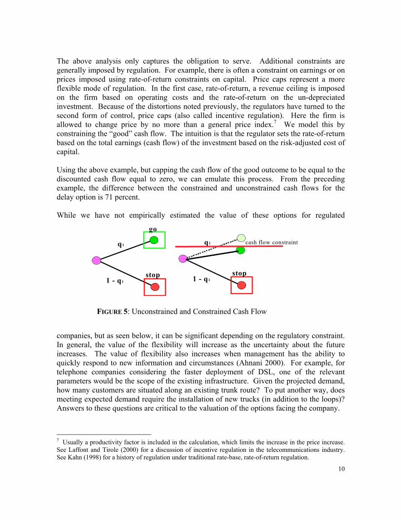
The above analysis only captures the obligation to serve. Additional constraints are generally imposed by regulation. For example, there is often a constraint on earnings or on prices imposed using rate-of-return constraints on capital. Price caps represent a more flexible mode of regulation. In the first case, rate-of-return, a revenue ceiling is imposed on the firm based on operating costs and the rate-of-return on the un-depreciated investment. Because of the distortions noted previously, the regulators have turned to the second form of control, price caps (also called incentive regulation). Here the firm is allowed to change price by no more than a general price index.7 We model this by constraining the “good” cash flow. The intuition is that the regulator sets the rate-of-return based on the total earnings (cash flow) of the investment based on the risk-adjusted cost of capital. Using the above example, but capping the cash flow of the good outcome to be equal to the discounted cash flow equal to zero, we can emulate this process. From the preceding example, the difference between the constrained and unconstrained cash flows for the delay option is 71 percent. While we have not empirically estimated the value of these options for regulated

companies, but as seen below, it can be significant depending on the regulatory constraint. In general, the value of the flexibility will increase as the uncertainty about the future increases. The value of flexibility also increases when management has the ability to quickly respond to new information and circumstances (Ahnani 2000). For example, for telephone companies considering the faster deployment of DSL, one of the relevant parameters would be the scope of the existing infrastructure. Given the projected demand, how many customers are situated along an existing trunk route? To put another way, does meeting expected demand require the installation of new trucks (in addition to the loops)? Answers to these questions are critical to the valuation of the options facing the company.

7 Usually a productivity factor is included in the calculation, which limits the increase in the price increase. See Laffont and Tirole (2000) for a discussion of incentive regulation in the telecommunications industry. See Kahn (1998) for a history of regulation under traditional rate-base, rate-of-return regulation.

q1

1 - q1stop

cash flow constraintq1

1 - q1

go

stop

FIGURE 5: Unconstrained and Constrained Cash Flow

11

A DELAY CRITERION8 With this background in mind, we now review an earlier result (Alleman, Sato, & Rappoport 2004, hereafter ASR) in order to apply the methodology to the model regulatory distortion by the inability to delay investment projects. Recall a financial option is the right to buy (a call) or sell (a put) a stock, but not the obligation, at a given price within a specific period of time. As noted, several approaches are possible to determine the theoretical value of an option, based on different assumptions concerning the market, the dynamics of stock price behavior, and individual preferences. Option pricing theory is based on the no-arbitrage principle, which is applied of the underlying stock’s distributional dynamics. The simplest of these theories is based on the multiplicative, binomial model of stock price fluctuations, which is often used for modelling stock behavior discussed earlier (also see ASR). To model the delay option, we utilize the continuously additive model developed by ASR which is review below. First we provided an example of the delay option, then we formally derive the option pricing formula which we use to derive the decision criterion statistic. We will use this to show the impact of the regulatory constraint on the investment decision.

Example: Value of the Option to Defer One real option alternative is the deferral option which is based on the concept of the call option, as shown in Figure 6 Luehrman (1998a). Consider a project, which is not currently profitable. A deferral option gives one the option to defer starting this project for one year to determine if the price increases enough to make the investment worthwhile. This right can be interpreted as a call option. The numerical example illustrates its value. Table 6 displays the project’s present value of future cash flow. V is assumed to be normally distributed with mean $100 million (= S) and standard deviation $30 million (= σ). The risk-free rate is 6% (R=1.06); the exercise price one year later is $110 million. With these assumptions, the project’s present value is $103.8 or $110/1.06.

Table 6 A projectDefer Option Variable

Present value of operating future cash flow S $100 millionInvestment in equipment K $103.8 millionLength of time the decision may be deferred T 1 yearRisk-free rate rf 1.06Riskiness s $30 million

Conventional NPV is given by S-K = 100 – 103.8 = - 3.8 million. This project would have been rejected under NPV criterion. However, applying call option formula in the pricing

8 This section is adapted from Alleman, Suto, & Rappoport (2004).

12

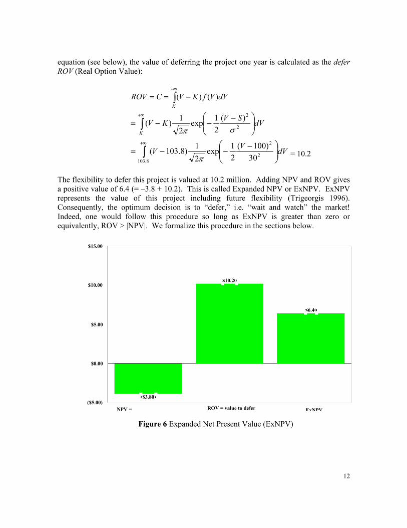
equation (see below), the value of deferring the project one year is calculated as the defer ROV (Real Option Value):

∫+∞

−==K

dVVfKVCROV )()(

∫+∞

−−−=

K

dVSVKV 2

2)(21exp

21)(

σπ

∫+∞

−−−=

8.1032

2

30)100(

21exp

21)8.103( dVVVπ = 10.2

The flexibility to defer this project is valued at 10.2 million. Adding NPV and ROV gives a positive value of 6.4 (= –3.8 + 10.2). This is called Expanded NPV or ExNPV. ExNPV represents the value of this project including future flexibility (Trigeorgis 1996). Consequently, the optimum decision is to “defer,” i.e. “wait and watch” the market! Indeed, one would follow this procedure so long as ExNPV is greater than zero or equivalently, ROV > |NPV|. We formalize this procedure in the sections below.

($3.80)

$10.20

$6.40

($5.00)

$0.00

$5.00

$10.00

$15.00

ExNPVNPV = ROV = value to defer

Figure 6 Expanded Net Present Value (ExNPV)

13

The Continuous Additive Model In the ASR model we normalize the net present value of the project by the standard

deviation i.e. '|'|

σImD −

= where m’ is the discounted cash flow, I is the initial investment

and σ′ is the standard deviation. In the standard case where '

'σ

ImD −= is less than zero

the investment is reject. With the real options methodology, one examines if the option value of delay “overcomes” the negative present value. What the ASR model does is solve for D at the point where the delay real option value is equal to normalized NPV, which is .278. This simple decision criterion determines, if NPV < 0, whether to “wait-and-watch” to see if the state of nature improves or to abandon the investment. Thus in the case of case of NPV < 0 the decision criterion is:

• ROV > |NPV| → Wait and watch the opportunity carefully; • ROV < |NPV| → Do not invest.

We derive this relationship as follows: Decision under conditions of uncertainty should be made on the basis of the current state of information available to decision makers. If the expectation of the NPV were negative for the investment, the conventional approach would be to reject the investment. However, if one has the ability to delay this investment decision and wait for additional information, the option to invest later has value. This implies that the investment should not be undertaken at the present time, but it leaves open the possibility of investing in the future.

Option pricing formula Consider

RuRSS += 01 (1) where

tS : stock price at time t u : normal distribution with mean 0, variance 2σ R : Return of risk-free asset or R = 1+rf (where rf is the risk-free rate of interest) per period.

A call option on this stock with exercise price = RK at time 1, payoff of option C(1) is:

)]0,[max()1( 1 RKSC −= i.e. 0)1( =C if RKS <1

RKSC −= 1)1( if RKS >1 (2) This option price can be calculated using the general option pricing formula.

14

)]([ˆ1 TCER

CT

= (3)

)]1([ˆ1 CER

=

11 )()1(1 dSSfCR ∫

+∞

∞−

=

where )( 1Sf is probability density function of S1, normally distributed.

111 )()(1 dSSfRKSR RK

∫+∞

−=

substituting RuRSS += 01 , )()/1()( 1 ufRSf = , RdudS =1 ,

∫+∞

−

−+=

0

)(1)(10

SK

RduufR

RKRuRSR

[ ]∫+∞

−

−+=0

)()( 0SK

duufKuS (4)

Assume uSV += 0 is normally distributed with mean 0S , variance 2σ , then (4) can be rewritten as a general option pricing formula for continuous model. Thus, the value of a one-period call option on a stock governed by a continuous additive model is

∫+∞

−=K

dVVfKVC )()( (5)

where V: the present value of the future random value discounted by risk-free rate K is the present value of exercise price, discounted by the risk-free rate This option formula will used below. Note that when V takes a lognormal distribution, this formula is equivalent to Black-Scholes call option formula (Herath and Park 2001).

15

V

Payo

ff, O

ptio

n Pr

ice

Prob

abili

ty

K =Exercise Price

Density Function of V

C

Payoff=C(1)

E [V ]

Figure 7 Option Price and Payoff This model can be extended to multi-period (T) options using the model:

tt

tt uRRSS += −1 (6)

where iu is the random variable normally distributed with mean 0, variance 2σ

i.e. ∑=

+=T

ii

TTT uRSRS

10 (7)

And assuming iu is not correlated with any other iju ≠ , the variance of PV[ E[ST ] ] is:

2

1

2 ]][[ σσ TuVarSPVVarT

iiTT =

=≡ ∑

= (8)

or

TTσσ = (9)

The one-term standard deviation can be calculated from multi-term one. The standard deviation of the yearly return is called volatility.9 When the return is defined as

]/[ 0SSPV T , its volatility is given by ( 0/ Sσ ). Although the option pricing theory has been developed in order to value financial options, it can be applied to the real asset or firm’s project. The next section shows how it is applied. Decision criterion statistic For the purpose of analyzing the relationship between NPV and the option value associated with the single investment, we assume that the random variable of interest is the present

9 A precise definition of volatility is “the standard deviation of the return provided by the asset in one year when the return is expressed using continuous compounding.” Hull (2003).

16

value of future cash flow V, which is assumed to be normally distributed V ~ N(m’, σ’). The investment cost I is assumed to be a constant. In the conventional method, NPV is expressed as:

NPV = E [V – I]

= E[V] – I

= m' – I (10)

Following Herath and Park (2001), we introduce a loss function. When no investment takes place, obviously, the cash flow is equal to 0. But imagine the situation that V > I, where the opportunity loss is recognized as V - I. Therefore the loss function is:

)(VL = 0, if V < I = V - I , if V > I

The expected opportunity loss can be calculated as:

∫+∞

∞−

= dVVfVLVLE )()()]([

∫+∞

−=I

dVVfIV )()(

This function is the payoff of a call option, using the pricing formula of a call option above (ASR). Assuming an investment can be deferred until new information is obtained, this value is the same as the defer option for the investment. Moreover, the value is also equal to the expected value of perfect information (EVPI) for this investment opportunity Herath and Park (2001) .

ROV = ∫+∞

−I

dVVfIV )()(

17

V

Loss

func

tion,

RO

V

Prob

abili

ty

I =Investment

Density Function of V

ROV

L(a 1 ,V )

m'

Figure 8 Opportunity Loss function and ROV (NPV<0) When the terminal distribution of V is normal, the real option value can be calculated using the unit normal linear loss integral:

∫+∞

−=D

NN dVVfDVDL )()()( (11)

where fN(V) is the standard normal density function

ROV = )(' DLNσ

Where '

|'|σ

ImD −= .

When a manager makes an investment decision, her optimal decision is not to invest if NPV = m'-I < 0. Then she may compare the NPV and the defer option value. If she finds that the option value is larger than the absolute value of NPV (= | m'-I |), she has the option to defer and watch for positive changes in the investment opportunity. If the option value is too small to compensate the NPV (< 0), she will abandon this investment proposal.

However, we can solve the equation,

ROV = |NPV|

18

From the above we derive the expression ImDLN −= ')('σ

Divided by σ‘, we have: (because σ‘ > 0)

'|'|)(

σImDLN

−=

ImDLN −= ')('σ (12) Divided by σ‘, we have: (because σ‘ > 0)

'|'|)(

σImDLN

−=

i.e. 0)( =− DDLN (13) Solving, D is:

0)( =− DDLN

0)()( =−−∫+∞

DdVVfDVD

N

0)()( =−− ∫∫+∞+∞

DdVVfDdVVVfD

ND

N

( ) 021exp

21 2 =−−−

− DDDD Φ

π

where ( ) ∫∞−

=a

N dxxfa )(Φ

∴ D = 0.278 And also the left hand side of equation (13) is decreasing as D increases because:

0))(( <− DDLdDd

N for all D > 0 (14)

What is the probability that the payoff of this defer option is positive if d = -D* at time 0? This can be calculated as follows,

>

′−

=>− 0]0[σ

IVPIVP

19

>

′−′+′−

= 0σ

ImmVP

′−′

−>′

′−=

σσImmVP

[ ]dNP −>= [ ]*DNP >=

= .39 where N is standard normal distribution.

Because V is N ~ (m’, σ‘), (V-m’)/ σ‘ is N~ (0, 1). Therefore, the probability that the payoff of the defer option is positive is 39%. Does it seem to be a high probability to abandon this option? Yes, it does! The criterion d < -D* means, “Do not invest now” but does not mean “Abandon the defer option.” The defer option itself has value though the expectation of NPV is deeply negative. If holding the option does not require any cost, it does not have to be thrown it away! Just wait and watch what happens in the next period. Below we as the above results to model the regulatory constraint.

REGULATORY DISTORTIONS MODELLED The impact of regulation can be simulated by constraining the variance. The price cap or discounted access charges or other regulatory devices dampen the possibility of a high return contract and this affects the variance of returns. Thus, the strength of the regulatory constraint can be modelled by constraining σ’. We do so by defining α as the regulatory

constraint on σ’, namely ασ’, which affects the decision statistic d = σ ′−′ Im . α lies

between zero and one (0 < α < 1), where 1 would represent no constraint on the regulated firm and zero would represent the most servere constraint on the firm. We then examine the probability of the real option is greater than or equal to the absolute value of the net present value as α varies between zero and one. We then examin a function that shows how the probability of the delayed option values is reduced as α varies. As intuition would suggest, as the constraint becomes tighter, the probability that the deferred option will pay-off is diminished. This is shown in Figure 9. As α approaches zero, the probability of the defer option being "in-the-money” is reduced significantly. This implies that the value of the investment will be reduced. Indeed, recall that the real option value can make the difference between waiting and watching to invest and abandoning the investment all together. Investments with negative discounted present value may be undertaken at a later date if the real option value is sufficient to overcome the negative NPV. As the regulatory constraint becomes tighter, this is less likely to occur.

20

0.00

0.05

0.10

0.15

0.20

0.25

0.30

0.35

0.40

0.45

1 0.9 0.8 0.7 0.6 0.5 0.4 0.3 0.2 0.1

alpha

proability

Figure 9 Probability delay options is greater than NPV as regulatory constraint increases.

SUMMARY We have shown that the introduction of uncertainty can make a significant difference in the valuation of a project. This manifests itself, inter alia, in the manner in which regulatory constraints can affect the value of the investment. In particular, the inability to exercise the delay, abandon, start/stop, and time-to-build options has an economic and social cost. Moreover, we show that regulatory constraints in cash flow have an impact on investment valuations. Regulators and policymakers cannot afford to ignore the implications and methods developed by real options analysis. Effective policy dealing with costs cannot be made without a fundamental understanding of the implications of real options theory. The real options approach is a powerful tool to be used to address the effect of uncertainty on regulatory policy. Real options methodology offers the possibility to integrate major analytical methods into a coherent framework that more closely approximates the dynamics of the firm’s behavior without heroic assumptions regarding the dynamics of the environment.

21

Applying real option valuation methodology shows that the new decision index d – the uncertainty adjusted NPV – and D* = 0.276 – the break-even point of NPV and ROV (real option value) – gives a clear solution to make a decision under uncertainty. When making decisions, managers have to observe only three parameters: expectation of future cash flow, its uncertainty, and the amount of investment to acquire the project. The examples using the new criterion show its usefulness.

FUTURE RESEARCH We plan to expand our work to empirically estimate the magnitude of the delay and other options. Another area we feel would be fruitful to explore is the issue of economic depreciation with these models. Clearly, (economic) depreciation is determined, inter alia, by the price the asset commands in the market (Hotelling 1925) and (Salinger 1998)). In contrast to others, we allow uncertain demand to set the optimal capacity path. Rather than assuming a user cost-of-capital, we can assume economic depreciation is determined endogenously by the demand function.

REFERENCES

1. AHNANI, M. & M. BELLALAH, “Real Options With Information Costs,” Working Paper, University of Paris-Dauphine & Université de Cergy, January 2000, pp. 1-22.

2. ALLEMAN, JAMES. “A New View of Telecommunications Economics,” Telecommunications Policy, Vol. 26, January 2002a, pp. 87- 92.

3. ALLEMAN, JAMES. “Irrational Exuberance?” The New Telecommunications Industry and Financial Markets: From Utility to Volatility Conference, 30 April 2002b.

4. ALLEMAN, J., The Poverty of Cost Models, the Wealth of Real Options, in Alleman and Noam (eds.), 1999, pp. 159-179.

5. ALLEMAN, J., “Real Options, Real Opportunities,” Optimize, Vol. 1, No. 2, January 2002c, pp. 57- 66.

6. ALLEMAN J., and PAUL RAPPOPORT. “Modelling Regulatory Distortions with Real Options” The Engineering Economics, volume 47, number 4, December 2002, pp. 390-417.

7. ALLEMAN, J. and E. NOAM (eds.), The New Investment Theory and its Implications for Telecommunications Economics, Regulatory Economics Series, Kluwer Academic Publishers, Boston, MA, 1999.

8. ALLEMAN J., HIROFUMI SUTO and PAUL RAPPOPORT. “An Investment Criterion Incorporating Real Options” Proceeding of the Eighth Annual International Conference on Real Options: Theory Meets Practice, Montreal Montreale, Canada, 17-19 June 2004.

9. AMRAM, MARTHA and NALIN KULATILAKA. Real Options, HBS Press, 1999 10. AVERCH H. and. LELAND L. JOHNSON, “Behavior of the Firm under a Regulatory

Constraint,” American Economic Review, Vol. 52, No. 5, 1962, pp. 1052-1069. 11. BIGLAISER G. and. M. RIORDAN, “Dynamics of Price Regulation,” RAND Journal of

Economics, Vol. 31, Issue 4 (winter), 2000, pp. 744-767. 12. BLACK F. AND M. SCHOLES, “The Pricing of Options and Corporate Liabilities,”

22

Journal of Political Economy, Vol. 81, 1973, pp. 637-659. 13. BOER, PETER. The Real Options Solution: Finding Total Value in a High-risk World,

John Wiley & Sons, Inc. 2002 14. DAMODARAN, ASWATH. Dark Side of Valuation, Prentice-Hall, 2001 15. COPELAND T. and V. ANTIKAROV, Real Options: A Practitioners Guide, Texere, New

York, 2001. 16. COX, J.C., S.A. ROSS and M. RUBINSTEIN, Options Pricing: A Simplified Approach,”

Journal of Financial Economics, No. 7, No. 3, 1979, pp. 229-264. 17. COPELAND, TOM and VLADIMIR ANTIKAROV. Real Options: A Practitioner’s Guide,

Texere LLC, 2001. 18. COPELAND, TOM, TIM KOLLER, and JACK MURRIN. Valuation: Measuring and

Managing the Value of Companies, McKinsey & Company Inc. 19. CRANDALL, ROBERT and LEN WAVERMAN (eds.), Who Pays for Universal Service:

When Subsidies Become Transparent, Brookings Institute Press, Washington, D.C., 2000. 20. D’HALLUIN, YANN, FORSYTH, PETER A., and KENNETH R. VETZAL. ”Wireless Network

Capacity Investment,” Proceeding of Real Options Seminar, University of Waterloo, Waterloo, Ontario, Canada 28 May 2004.

21. D’HALLUIN, YANN, FORSYTH, PETER A., and KENNETH R. VETZAL. “Managing Capacity for Telecommunications Networks,” Proceeding of Real Options Seminar, University of Waterloo, Waterloo, Ontario, Canada 28 May 2004.

22. DIXIT A. and R.S. PINDYCK, Investments Under Uncertainty, Princeton University Press, NJ, 1994.

23. DIXIT A. and R.S. PINDYCK, “The Options Approach to Capital Investments,” Harvard Business Review, Vol. 73, No. 3, May-June 1995, pp.105-115.

24. ERGAS H. and J. SMALL. “Real Options and Economic Depreciation,” NECG Pty Ltd and CRNEC, University of Auckland, 2000.

25. HAUSMAN JERRY. “The Effect of Sunk Cost in Telecommunications Regulation,” in Alleman and Noam (eds.), The New Investment Theory and its Implications for Telecommunications Economics, Regulatory Economics Series, Kluwer Academic Publishers: Boston/Dordrecht/London, 1999, pp. 191-204.

26. HAUSMAN JERRY. “Competition and Regulation for Internet-related Services: Results of Asymmetric Regulation,” in Alleman and Crandall (eds.). Broadband Communications: Overcoming the Barriers, 2002.

27. HERATH, S.B. HEMANTHA, and CHAN S. PARK, “Economic Analysis of R&D Projects: An Option Approach,” The Engineering Economist, Vol. 44, No. 1, 1999, pp. 1-32.

28. HERATH, S.B. HEMANTHA, and CHAN S. PARK, “Real Options Valuation and Its Relationship to Bayesian Decision Making Methods,” The Engineering Economist, Vol. 46, No. 1, 2001, pp. 1-32.

29. HORI, KEIICHI and KEIZO MIZUNO. “Network Investment and Compettion with Access to Bypass,” Proceeding of the Eighth Annual International Conference on Real Options: Theory Meets Practice, Montreal Montreale, Canada, 17-19 June 2004.

30. HOTELLING H., “A General Mathematical Theory of Depreciation,” Journal of the American Statistical Association, Vol. 20, September 1925, pp. 340-353.

31. HULL, J.C., Options, Futures and other Derivatives, 4th ed., Prentice-Hall, Upper

23

Saddle River, NJ, 2000. 32. KAHN, ALFRED E., The Economics of Regulation: Principles and Institutions, Volume I

and II, Cambridge, MA: MIT Press; and New York: Wiley, 1988. 33. KULATILAKA, NALIN, and LIHUI LIN. “Strategic Investment in Technological

Standards,” Proceeding of the Eighth Annual International Conference on Real Options: Theory Meets Practice, Montreal Montreale, Canada, 17-19 June 2004.

34. LAFFONT, J-J. and TIROLE, J., Competition in Telecommunications, Cambridge, MA: MIT Press, 2000.

35. LUENBERGER, D.G., Investment Science, Oxford University Press, 1998. 36. LUEHRMAN, TIMOTHY. Investment Opportunities as Real Options: Harvard Business

Review, 51-67, July-August 1998a 37. LUEHRMAN, TIMOTHY. Strategy as a Portfolio of Real Options: Harvard Business

Review, 89-99, September-October 1998b 38. MAUBOUSSIN, MICHAEL. Get Real, Credit Suisse Equity Research, June 1999. 39. NEMBHARD, HARRIET BLACK, LEYUAN SHI and CHAN S. PARK, “Real Option Models

For Managing Manufacturing System Changes in the New Economy,” The Engineering Economist, Vol. 45, No. 3, 2000, pp. 232-258.

40. NOAM E., “How Telecom Is Becoming A Cyclical Industry, And What To Do About It,” The New Telecommunications Industry and Financial Markets: From Utility to Volatility Conference, 30 April 2002.

41. PAK, DOHYUN and JESSI KEPPO. “A Real Options Approach to Network Optimization,” Proceeding of the Eighth Annual International Conference on Real Options: Theory Meets Practice, Montreal Montreale, Canada, 17-19 June 2004.

42. PARK, CHAN S., “Taking Engineering Economy to the Next Level: An editorial note,” The Engi0neering Economist, Vol. 44, No. 1, 1999, pp. i-ii.

43. PARK, CHAN S. and HEMANTHA S.B. HERATH, “Exploiting Uncertainty –Investment Opportunities as Real Options: A New Way of Thinking in Engineering Economics,” The Engineering Economist, Vol. 45, No. 1, 2000, pp. 1-36.

44. SALINGER M. “Regulating Prices to Equal Forward-Looking Costs: Cost-Based Prices or Price-Based Costs,” Journal of Regulatory Economics, Vol. 14, No. 2, September 1998, pp. 149-164.

45. SCHLAIFER, ROBERT. Introduction to Statistics for Business Decisions, McGraw Hill, 1961.

46. SMALL JOHN P., “Real Options and the Pricing of Network Access,” 1998, CRNEC Working Paper available at http://www.crnec.auckland.ac.nz/research/wp.html

47. SMITH, JAMES E. and ROBERT F. NAU, “Valuing Risky Projects: Option Pricing Theory and Decision Analysis,” Management Science, Vol. 41, No. 5, May 1995, pp. 795-816.

48. TAUKE TOMAS J., Testimony of Thomas J. Tauke Before the Committee on the Judiciary United States House of Representatives, 2001.

49. TRIGEORGIS LENOS. Real Options Management Flexibility and Strategy in Resource Allocation, MIT Press: Cambridge, MA., 1996.

50. YAMAMOTO, DAISUKE. Introduction to Real Options, Toyo-Keizai, 2001 (in Japanese)