Teknisk-naturvetenskapliga fakulteten Examensarbete i matematisk statistik D-nivå, 20 poäng

Modelling Operational Risk using

Actuarial Methods

Marcus Larneback

Institutionen för matematik och matematisk statistik Umeå universitet 901 87 UMEÅ

Modelling Operational Risk using

Actuarial Methods

Marcus Larneback

Examensarbete i matematisk statistik

D-nivå, 20 poäng

Maj 2006

Marcus Larneback: Modellering av operationella risker med försäkringsmatematiska metoder Institutionen för matematik och matematisk statistik, Umeå Universitet, 901 87 Umeå © Marcus Larneback, 2006 Detta arbete har skrivits för avläggande av filosofie magisterexamen i ämnet matematisk statistik. Arbetet har gjorts på D-nivå och omfattar 20 poäng. Handledare: Kaj Nyström Examinator: Peter Anton Marcus Larneback: Modelling Operational Risk using Actuarial Methods Department of Mathematics and Mathematical Statistics, Umeå University, 901 87 Umeå © Marcus Larneback, 2006 This is a thesis for the degree of Master of Science in Mathematical Statistics. Supervisor: Kaj Nyström Examiner: Peter Anton

Modelling operational risk using

actuarial methods

Marcus Larneback

Master Thesis

Department of Mathematical Statistics

Umea University

SE-901 87 Umea, Sweden

Abstract

Within the financial industry Operational Risk is a relatively new concept, butwithin recent years it has gained more attention due to prior economically devastatingevents; these are events that cannot be categorized as market- or credit risks. Thepurpose of this thesis is to study the Loss Distribution Approach(LDA). This is one ofthe more rigorous models proposed by the Basel Committee on Banking Supervision,in order to calculate the required capital charge that should be set aside to cover futureoperational loss events within financial institutions. The focus is on the close connec-tion between the LDA and modelling techniques which are used in the field of insurancemathematics. A summary of relevant theoretical results underlying the (aggregate) lossdistribution is given, and then detailed ways to model the specific components are pro-vided. More specifically, certain techniques are emphasized, for example: extreme valuetheory are used to model certain loss severities; and also generalized linear models areused to link event frequency to possible causes, thereby also allow for scenario-basedmodelling. The models are illustrated in a numerical example where parameter calibra-tion and exploratory techniques are addressed, and several useful tools are identified.Finally capital charges in terms of VaR and CVaR measures are numerically calculatedand compared with asymptotic approximations.

Sammanfattning

Operationell risk ar ett relativt nytt begrepp inom den finasiella industrin menhar de senaste aren fatt alltmer uppmarksamhet till foljd av specifika handelser somhaft en forodande ekonomisk effekt for den enskilda orgnisationen. Dessa handelserhar dock inte kunnat klassas som marknads- eller kredit-risker. I detta examensar-bete studerar vi Loss Distribution Approach(LDA) vilken ar en av de mer avancerademetoder som foreslagits av Basel Committee on Banking Supervision for att beraknadet kapital som behovs for att tacka framtida operationella forluster inom finasiellainstitut. I synnerhet fokuserar vi pa likheter mellan LDA och metoder som anvandsinom forsakringsmatematiken. Vi ger en sammanfattning av teoretiska resultat kop-plade till den totala forlust-fordelningen och diskuterar mojliga ansatser for att estimeradess ingaende komponenter. Mer specifikt anvands tekniker fran extremvardesteorienfor att modellera vissa typer av forluster och generaliserade linjara modeller for attkoppla samman forlust-frekvens med mojliga orsaksfaktorer for att pa sa vis avenmojliggora scenario-analys. Modellerna illustreras genom ett numeriskt exempel medfokus pa parameter-skattning och anvandbara grafiska redskap. Slutligen beraknas kap-italtackningskrav utifran riskmatten VaR och CVaR numeriskt, for att sedan jamforasmed asymptotiska approximationer.

Contents

1 Introduction 1

2 The Data 5

3 Measures of Risk 8

4 Loss Distribution Approach 104.1 The counting process . . . . . . . . . . . . . . . . . . . . . . . . . . . . . 104.2 The compound model . . . . . . . . . . . . . . . . . . . . . . . . . . . . 114.3 Loss distributions . . . . . . . . . . . . . . . . . . . . . . . . . . . . . . . 12

5 Extreme Value Theory 165.1 Asymptotics of extremes . . . . . . . . . . . . . . . . . . . . . . . . . . . 165.2 Generalized Pareto distribution . . . . . . . . . . . . . . . . . . . . . . . 17

6 Numerical Evaluation of the Compound Sum 196.1 Panjer recursion . . . . . . . . . . . . . . . . . . . . . . . . . . . . . . . 196.2 Methods of arithmetization . . . . . . . . . . . . . . . . . . . . . . . . . 21

7 Generalized Linear Models 237.1 Exponential family of distributions . . . . . . . . . . . . . . . . . . . . . 237.2 Generalized linear model . . . . . . . . . . . . . . . . . . . . . . . . . . . 237.3 Poisson regression and log-linear models . . . . . . . . . . . . . . . . . . 25

8 Application 278.1 Frequency modelling . . . . . . . . . . . . . . . . . . . . . . . . . . . . . 278.2 Loss modelling . . . . . . . . . . . . . . . . . . . . . . . . . . . . . . . . 318.3 Stress testing and evaluation of risk measures . . . . . . . . . . . . . . . 358.4 Software . . . . . . . . . . . . . . . . . . . . . . . . . . . . . . . . . . . . 38

9 Summary and Conclusions 39

1 Introduction

Parallel to the technological advancement of recent times banks today have developedinto complex high technological apparatus relying heavily, not only, on the competenceof its manpower, but also on the intricate technical systems and numerous external fac-tors. In such an environment many possible sources of risk exist; computer breakdowns,transaction errors and temporary loss of staff, to mention a few. This has indiscerniblycaused banks, and indirectly their customers and shareholders, considerably financialdamage. Though, it is the more spectacular events, like a single man’s unauthorizedtrading at a small Singapore office within the Barings Bank’s, that has attracted massmedia attention and opened the eyes of the regulatory authorities.

The recognition of Operational Risk exposure, being a substantial and growingpart in the business of financial institutions, has led the Basel Committee on BankingSupervision to include a new capital requirement within the New Basel Capital Accord.The purpose is to develop a minimum regulatory capital charge for other risk, includingoperational risk. Historically, Operational risk has implicitly been covered by CreditRisk, which is associated with the uncertainty that debtors will honor their financialobligations. Alongside credit risk, the risk associated with fluctuations in the value oftraded assets, known as market risk, have been the two risk categories used to subdividethe overall risk faced by institutions.

In cooperation with the financial industry, representatives of the working group forthe committee have established the following definition of operational Risk:

Definition 1 (Operational risk) The risk of loss resulting from inadequate or failedprocesses, people and systems or from external events.

This definition includes legal risk but excludes strategic and reputational risk, and theintention is not to cover all indirect losses or opportunity costs. It is based on theunderlying causes of operational risk and seeks to identify why a loss has happenedand at the broadest level includes the breakdown by four causes: people, processes,systems and external factors. For more information on the subject of the regulatoryevolvement one may consult the BIS publications Consultative document (2001) andthe Working paper on the regulatory treatment of operational risk (2001). With thesepublications the committee intended to further deepen the dialogue with the industryand left the ball in their court to reflect and return with suggestions and improvements.Since then several contributions are left up for debate and some useful references areFrachot et al. (2001) and Embrechts et al. (2004).

In the papers presented above the general belief seems to be that organizations willstrive towards advanced measurement approaches, which will allow the use of outputfrom internal operational risk measurement systems. The intention of initiating such asystem should be twofold. Not only should the system in a quantitative sense generatemathematically sound and optimally calibrated risk capital charges, but also give anincentive to create robust controls and procedures to support active management ofoperational risk. Hence, operational risk should also be modelled in such a way thatcauses are identified. This has been acknowledged by Ebnother et al. (2001) whoapproaches the problem through the definition of certain work flow processes in a

1

graph structure, and estimates the impact on risk figures through different choices ofrisk factors. Also addressing this matter Nystrom & Skoglund (2002) stress the needof extending proposed basic models to incorporate the concept of key risk drivers,and outline both direct and indirect approaches. Thirdly, Cruz (2002) devotes severalchapters to describing common econometric and non-linear models that can be usedfor this matter.

A source of concern in the industry is presently the limited access to reliable op-erational loss data. One natural reason for this is confidentiality. Secondly, there hasbeen no set industry standard for consistent gathering of the data. Existing databasesconsist of data from a relatively short historical period and is often of poor quality. De-spite the latter problems, different loss characteristics have been observed within theindustry. Bank’s internal data are biased towards low severity losses like transactionfailures, credit card frauds and accounting irregularities. These tend to occur frequentlybut cause relatively small losses. On the contrary, when observing the losses within anindustrial wide context, loss events that very clearly show extreme outcomes but occurwith a low frequency are highlighted. For that reason pooling of data across banks hasbeen discussed. Pros and cons of such methods, within the context of operational risk,are considered in Frachot et al. (2002). Under the advanced measurement framework,operational risk exposure and losses are due to the proposed features, categorized intostandardized business lines and event types. This is done according to an industrystandard matrix, which is designed to be generally applicable across a wide range ofinstitutions.

The model which has gained the most interest within the advanced measurementframework is the Loss Distribution Approach(LDA). A well known analogue to theLDA, within the field of actuarial mathematics, is the probabilistic interpretation ofthe random sum

S(t) = X1 +X2 + . . .+XN(t),

stemming from a random process generating claims for a portfolio of insurance policiesin a given period of time. Under the LDA, the institutions will estimate the totaloperational loss for each business line/event type, or grouping thereof, in a fixed fu-ture planning period. This means estimating the probability distributions of both thenumber of loss events and the severity of individual events using primarily its inter-nal data. The aggregate loss(compound-) distribution can then be expressed in termsof convolutions of the individual loss distribution functions. In general, no analyticalexpression of the aggregate loss distribution exist.

The thesis aims to provide a review for some applicable actuarial methods withinthe LDA, to the modelling of operational risk under the assumption of independentand identically distributed losses. First, we want to perceive a broader understandingof the compound model and its building blocks from a theoretical aspect. From arisk measurement viewpoint it is the tails of loss distributions which are of particularinterest. Thus, in regard to the different characteristics observed in empirical lossdata, as described above, special theoretical emphasis will be given to the influenceof different loss distribution assumptions on the tail of the compound distribution.This theoretical area turns out to be closely connected to extreme value theory, whichis an important tool when dealing especially with heavy tailed data, and therefore

2

deserve separate treatment. Even though the asymptotic theorems outlines a way todirect approximation of risk measures, we need to investigate when these formulasbecome sufficiently accurate. Therefore, computation of the aggregate loss distributionis necessary and requires a numerical algorithm. The Panjer recursion approach willbe used for this purpose.

Additionally, one(among many) possible approach(-es) to casual analysis and theidentification of potential risk factors are considered. Assuming proper reporting andclassification systems are in place, causal analysis will be the next step in the riskmanagement process. Understanding the source of losses is fundamental in trying toavoid them. Hence, staff turnover, overtime and number of transactions, to mention afew examples, may be relevant factors in identifying and forecasting future loss events.Within the scope of the thesis, only frequency risk factors will be considered. Thebasis will be the multi-factor/regression approach known as generalized linear mod-elling(GLM). The class of GLMs is an extension of the classical linear models in theform

E(Yi) = µi = xTi β; Yi ∼ N(µi, σ

2), (1.1)

where the following generalizations are made:

1. Response variables may have distributions other than the Normal distribution.They may even be categorical rather than continuous.

2. The relationship between the response and explanatory variables need not to beof the simple linear form, as in (1.1).

GLMs have found their way in several actuarial applications such as premium ratingand loss reserving. They can be extended in various ways to account for time-seriesstructures as well as inclusion of random effects, and therefore provide a good base formore sophisticated models.

In a numerical example we analyze two fictive cells in the regulatory matrix using theproposed models. We restrict the thesis towards assessments concerning such individualcells. For discussions about capital allocation and total capital charges for the bank asa whole, we refer to Frachot et al. (2001). The main purpose of the data analysis isto gain some insight about exploratory tools used to fit parametric loss distributions.Furthermore, the factor approach results in estimates of loss frequency and we are ableto calculate risk measures under different assumptions of future exposure to risk factors.Due to the lack of appropriate operational risk data, the numerical illustration will begiven using insurance data. This is in line with Embrechts et al. (2004) that concludesthat operational risk data are in many ways akin to property insurance loss data.This data has been collected from the insurance company If and will be presented insection 2. The two data sets consists of claims data for two different types of coveragein a car-insurance contract. They are chosen specifically to illustrate the differentcharacteristics, as addressed above, that one may face when modelling loss data. Somerelated covariates(i.e. risk factors) are also available. Figures and comments in thethesis do not represent the views and/or opinions of the If management, and the riskmeasures and other estimates are purely of an illustrative purpose.

3

The rest of the thesis will be organized as follows. Section 3 gives a brief backgroundand definitions of two common measures of risk used in finance, in order to quantifythe amount of the capital charge needed. Section 4 gives an theoretical overview of theloss distribution approach. In direct connection to the theoretical aspects of loss dis-tributions in subsection 4.3, a background to Extreme Value Theory is given in section5. The two following sections separately details the models discussed above, startingwith the Panjer Recursion approach in section 6 and followed by the Generalized LinearModel in section 7. In section 8, appropriate tools for model selection and parametercalibration to the data sample will be addressed through the numerical illustration,which is followed by stress testing and evaluation of risk measures. Finally, section 9contains a summary of the results and a further discussion of the problems and possibleextensions, in contrast to the models used.

4

2 The Data

The data analyzed in the thesis is car-insurance data, collected under a five-year periodfrom the 1st of January, 2000, to the 31st of December, 2004.

The first data set consists of personal injury claims. Personal injury(PI) is one partof the Third party liability coverage, which in Sweden is mandated by law. This coversthe policy-owner and his/her passengers, as well as third party, against damages suchas medical expenses, lost wages and pain and suffering.

The second data set originates from Motor Rescue(MR), which is one element ofthe Partial cover coverage, also including for example theft and fire. Motor rescue isessentially a breakdown service designed to assist the policy-holder with the necessaryprocedures, in the event of breakdown or accident, or in the case of illness or death.

For the sake of integrity, the amount of the claims are multiplied by unspecifiedscaling factors. A graphical summary of the two data sets is given in figure 1. Thex-axis in the histograms are shown on a log scale to emphasize the great range of thedata. Summary statistics are given in table 1.

5

2000-01-01 2000-12-31 2001-12-31 2002-12-31 2003-12-31 2004-12-31

Time

0

2000

4000

6000

8000

2000-01-01 2000-12-31 2001-12-31 2002-12-31 2003-12-31 2004-12-31

Time

0

2

4

6

8

-4.0 -2.6 -1.2 0.2 1.6 3.0 4.4 5.8 7.2 8.6 10.00

10

20

30

-6.0 -5.1 -4.2 -3.3 -2.4 -1.5 -0.6 0.3 1.2 2.1 3.00

10

20

30

40

Figure 1: Time series plot and log data histograms for PI and MR claims respectively.

Table 2 shows a list of selected covariates commonly used in car-insurance ratingand the corresponding number of classes. Their exact meaning is not important inthis context and due to confidentiality they will therefore be named A, B, C and Drespectively. For the same reason the banding of these rating factors are deliberatelyleft ill defined. The number of claims and the corresponding exposure(i.e. total numberof years insured) is given, however only the former is shown.

6

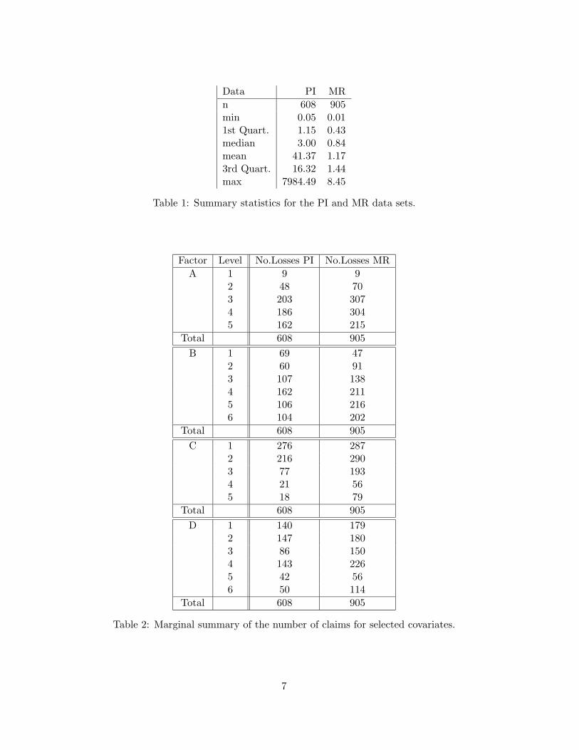
Data PI MR

n 608 905min 0.05 0.011st Quart. 1.15 0.43median 3.00 0.84mean 41.37 1.173rd Quart. 16.32 1.44max 7984.49 8.45

Table 1: Summary statistics for the PI and MR data sets.

Factor Level No.Losses PI No.Losses MR

A 1 9 92 48 703 203 3074 186 3045 162 215

Total 608 905

B 1 69 472 60 913 107 1384 162 2115 106 2166 104 202

Total 608 905

C 1 276 2872 216 2903 77 1934 21 565 18 79

Total 608 905

D 1 140 1792 147 1803 86 1504 143 2265 42 566 50 114

Total 608 905

Table 2: Marginal summary of the number of claims for selected covariates.

7

3 Measures of Risk

For a long time the concept of Value at Risk has been adapted in the financial industryas best practice. The Value at Risk is taken to be the (right-) quantile, qα, of the lossdistribution and is thus defined as

Definition 2 (Value at Risk) Let α be fixed and X a real random variable, then

V aRα(X) = qα(X) = inf{x ∈ R : P [X ≤ x] ≥ α} (3.1)

is called the Value at Risk(VaR) at (confidence-) level α of X.

Thus stating that it is the smallest value, such that the probability of the loss taking atmost this value is at least 1 − α. Throughout the thesis, losses are defined as positivereal numbers.

Among market participants1 and for the sake of regulating authorities, it is of courseof outmost importance to have a unified view of the measures of risk. In 1997, Artzeneret al. presented a framework and tried to give a clear definition of the properties that aneffective tool of measurement should possess. As the basis for their argumentation theystated four axioms and they called every risk measure fulfilling these axioms coherent.

Definition 3 (Coherent risk measure) Consider a set V of real-valued random vari-ables. A function ρ : V → R is called a coherent risk measure if it is

(i) monotonous: X ∈ V,X ≥ 0 ⇒ ρ(X) ≤ 0,

(ii) sub-additive: X,Y,X + Y ∈ V ⇒ ρ(X + Y ) ≤ ρ(X) + ρ(Y ),

(iii) positively homogeneous: X ∈ V, h > 0, hX ∈ V ⇒ ρ(hX) = hρ(X), and

(iv) translation invariant: X ∈ V, a ∈ R⇒ ρ(X + a) = ρ(x) − a.

Many examples can be given that the VaR measure does not fulfill the sub-additiveproperty and hence is not supporting risk-diversification in a portfolio. Another draw-back is that VaR is not law-invariant, meaning that we can easily find random vari-ables X and Y such that for some t = tl, P [X ≤ tl] = P [Y ≤ tl] without implyingρ(X) = ρ(X) for all t ∈ R. A proper choice lying within the class of coherent riskmeasures turn out to be Conditional Value at Risk.

Definition 4 (Conditional Value at Risk) Let α ∈ (0, 1) be fixed and let X be areal random variable with E[max(0, X)] <∞ Then

CV aRα(X) = (1 − α)−1

(

E[X 1{X≥V aRα(X)}]

+V aRα(X)(

α− P [X > V aRα(X)])

)

(3.2)

1By market participants we intend all actors in the financial industry undertaking some kind ofregulatory capital allocation in their business.

8

with indicator function 1A defined as

1A(x) =

{

1, x ∈ A

0, x /∈ A.

is called the Conditional Value at Risk(or Expected Shortfall) at a level α of X.

In case the random variable X has a continuous distribution function, the above defi-nition gives the more manageable expression

CV aRα(X) = E[X | X > V aRα(X)]. (3.3)

The Conditional Value at Risk has a couple of possible interpretations. The mostobvious interpretation, is that it can be thought of as the ”average loss in the worst100(1 − α)% cases”. It can also be shown as the integral over all quantiles above thevalue u.

Theorem 1 (Integral representation of CVaR) For CV aRα as defined in (1.2)and V aRα as given in (1.1), we have

CV aRα(X) =1

1 − α

∫ 1

αV aRα(X)du

whenever X is a real random variable with E[max(0, X)] <∞.

This is an implication of a theorem in Delbaen (1998), where it was shown that allcoherent risk measures may be seen as integrals over VaR-numbers. For the continuousrandom variable X, the conditional Value at Risk is the smallest coherent and law-invariant risk measure that dominates VaR. Moreover, Kusuoka (2001) has shown thatit constitutes the basis of any law invariant measure of risk. In section 8.2 it will beseen that the expected shortfall function is a useful analytical tool in the exploratorydata analysis of large losses.

In finance, the risk measures may be superscripted, i.e. V ARtα, indicating the t-day

holding period of the instrument. Throughout this context, we will always consider afixed planning period and thus the superscript will not be necessary.

9

4 Loss Distribution Approach

4.1 The counting process

In the non-life insurance industry it is, as a first step, usually assumed that the claimsoccur as a sequence of events in such a random way that it is not possible to forecastthe exact time of occurrence of any one of them, nor the exact total number.

Consider the accumulated number N(t) of claims occurring during a time periodfrom 0 to t as a function of a fixed time t, then N(t) is a stochastic process. It is well-known in probability theory that if the following statements can be accepted about theclaim number process:

• The number of claims occurring in any two disjoint time intervals are independent

• The number of claims in a time interval is stationary (i.e. dependent only on thelength of the interval)

• No more than one claim may arise from the same event

Then when put in definition in a mathematical setting, Gut (1995), we have a homo-geneous poisson process:

Definition 5 (Poisson process) A poisson process {N(t), t ≥ 0} is a nonnegative,integer-valued stochastic process such that N(0) = 0 and

1. the increments {N(tk) −N(tk−1), 1 ≤ k ≤ n} are independent; and

2. P(exactly one occurrence during (t,t+h])=λh + o(h) as h → 0, for some λ > 0;and

3. P(at least two occurrences during (t,t+h])=o(h) as h→ 0.

Making use of these conditions it is then proved that the number of claims, n, in agiven fixed time interval of length tp = [tk−1, tk] is Poisson distributed as

pn = Prob{N = n} = pn(λtp) = eλtp (λtp)n

n!

and intensity parameter λ. Again, with λ we intend the expected number of losses ina fixed planning period and we can set tp = 1.

For most cases in reality there may, of course, be objections to (all of) the statementsabove. For example, in car-insurance seasonal weather conditions affecting the risk maydiffer significantly from year to year. It is also likely that traffic accidents is dependingon the state of the general economy(i.e. economic booms tend to increase the trafficintensity which in turn leads to more accidents).

In a short-term perspective, when the fluctuation within the planning period isconsiderable but can be regarded as independent between consecutive years, it is oftenincorporated into the claim frequency process by modelling λ as a random variable Λ

10

(i.e. mixed poisson) with corresponding probability density function h(x). Then wehave N ∼ Po(Λ) and

E(N) = E[E(N | Λ)] = E(Λ),

V ar(N) = E[V ar(N | Λ)] + V ar[E(N | Λ)],

and henceV ar(N) = E(Λ) + V ar(Λ).

For the case Λ = λ, a constant, the moments of the poisson, E(N) = V ar(N) = λ,are reproduced. We see that V ar(N) > E(N), which is a phenomena referred to asover-dispersion of the process {N(t)}. Indisputably, the most common choice of h(x)is the gamma distribution which leads to N being negative binomial distributed.

The poisson process suffers from some limitations but can in practice often givea first good approximation, and the assumption that the number of claims obeys apoisson distribution in a fixed planning period will be made in the thesis. The negativebinomial model is an interesting and important alternative, however other extensionsof the basic model might be needed, and further references are given in section 7.2.

4.2 The compound model

The foundation is laid by proposing a probability distribution for the claim numberrandom variable, and now turn our focus to the complete model, which the thesis isconcerned about. We start by introducing the following definition from Nystrom &Skoglund (2002).

Definition 6 (Compound counting process) A stochastic process{S(t), t ≥ 0} is said to be a compound counting process if it can be represented as

S(t) =

N(t)∑

k=1

Xk, t ≥ 0,

where {N(t), t ≥ 0} is a counting process and the {Xk}∞1 are independent and identi-

cally distributed random variables, which are independent of {N(t), t ≥ 0}.

Given a fixed time interval, the compound(aggregate) loss distribution can be written

G(x) = P (S ≤ x) =∞

∑

n=0

pnFn∗(x), (4.1)

where Fn∗(x) = P (∑n

i=1Xi ≤ x) is the n-fold convolution of F and F 0∗(x) ≡ 1.The moments of the compound loss distribution are particularly simple in the com-pound poisson case. If we let

αr = E(Xr) =

∫ ∞

0zrdFX(z)

11

denote the rth moment about the origin for the loss random variable X, then by con-ditional expectation we obtain the following expressions for the mean,

E[S] = E[E[S | N ]] = E[E(X)N ] = α1λ,

variance

V [S] = V [E[S | N ]] + E[V [S | N ]] = V [E[X]N ] + E[V [X]N ] =

= α21λ+ (α2 − α2

1)λ = α2λ,

and skewness

γ[S] =E[(S − α1λ)3]

V [S]3/2=

α3λ

(α2λ)3/2=

α3√

(α2)3λ.

The compound poisson model has an interesting additive property which allows forany collection, Sj , j = 1, . . . , n of independent compound Poisson random variableswith corresponding intensity parameters λj and loss distributions Fj to be treated asa single compound risk. It is shown that S =

∑nj=1 Sj is again compound poisson with

intensity λ =∑n

j=1 λj and loss distribution FX(x) =∑n

j=1λj

λ Fj(x).

4.3 Loss distributions

In classical risk theory focus of attention has been the modelling of the surplus process(U(t))t≥0 in a fund(i.e. a portfolio of insurance policies) defined as

U(t) = u+ ct− S(t), t ≥ 0,

where u ≥ 0 denotes the initial capital, c > 0 stands for the premium income rateand S(t) is a compound counting process as defined in definition 6. In the famousCramer-Lundberg model S(t) is a compound poisson process. One possible measure ofsolvency in the fund, of special importance in actuarial ruin theory, is the probability ofruin ψ(u, T ) = P (U(t) < 0 for some t ≤ T ), 0 < T ≤ ∞. That is, the probability thatthe surplus in the fund becomes negative in finite or infinite time. Under a conditionof ”small claims”, the so called Cramer-Lundberg estimate for the probability of ruinin infinite time, yields bounds which are exponential in the initial capital u, as

ψ(u,∞) < e−Ru, u ≥ 0. (4.2)

We will not go further into the estimation of ruin probabilities and calculations ofappropriate premium flows, and refer to Grandell (1991) for details. Instead we willproceed with focus on S(t), having the small-claim condition above in mind. This posesthe question,

- What is to be considered as a ”small” claim(loss)?

But more importantly,

- Is it possible to classify loss distributions in order to their influence on the (tailof the)aggregate loss distribution?

12

1 2 3 4 5

Exponential

0

20

40

60

80

100

120

1 2 3 4 5

Lognormal

0

50

100

150

Figure 2: Five largest total loss amounts divided into its individual loss amounts in asimulation of n = 1000 losses.

Before jumping to the theoretical results, we will try to get an intuitive idea througha graphical illustration of the difference in ”building blocks” for the tails of compounddistributions.

Figure 2 shows the five largest total loss amounts in simulations of two differentcompound loss distributions. The counting random variable is poisson distributed,with the same expected number of losses(λ = 10) in both cases. But one with anexponential(with parameter ρ = 4) loss distribution, and one with a log-normal(withparameters µ = 0.886 and σ = 1) loss distribution, giving the same expected value ofE(X) = 4. It is clear that in the exponential case the most severe aggregate losses aredue to a higher(extreme) intensity outcome, whereas in the log-normal case we observelarge losses that tend to overshadow the many smaller ones.

Theoretical results answering the questions stated above can be found in Embrechtset al. (1985) and Embrechts et al. (1997), and the rest of this section will give a shortsummary. In the classical model above, the condition on the loss distribution leading tothe existence of R > 0 in (4.2) can be traced back to the existence of the (real-valued)Laplace transform, or moment generating function with v interchanged with −s,

LX(v) = E(e−vX) =

∫ ∞

0e−vxdF (x), v ∈ R

which typically holds for distributions with exponentially bounded tails. It is shownthrough Markov’s inequality that

F (x) ≤ e−sxE(esX), x > 0,

where 1 − F (x) = F (x) in the following will be used interchangeable to denote thetail of the distribution. This inequality means that large claims are very unlikely tooccur, i.e. with exponentially small probabilities. Probability distributions with thisproperty is referred to as light-tailed. Light-tailed distributions which historically havebeen considered in an insurance context, is for instance the exponential, the gamma,and the light-tailed(τ ≥ 1) Weibull. A good reference for insurance claim distributionsis Hogg & Klugman (1984).

13

When heading towards asymptotical formulas for the compound loss distribution,we first need to be familiarized with the following definition.

Definition 7 (Slowly varying function) A function C(x) is said to be slowly vary-ing at ∞ if, for all t > 0,

limx→∞

C(tx)

C(x)= 1.

Typical examples of slowly varying functions are functions converging to a positiveconstant, logarithms and iterated logarithms. Furthermore, a function h(x) is saidto be regularly varying at ∞ with index α ∈ R if h(x) = xαC(x). Then the followingtheorem given in Embrechts et al. (1985) gives asymptotical formulas for the compoundloss.

Theorem 2 (Compound loss in the light-tailed case) Suppose pn satisfies

pn ∼ θnnγC(n), n→ ∞ (4.3)

for 0 < θ < 1, γεR and C(x) slowly varying at ∞. If, in addition, there exists a numberκ > 0 satisfying

θ−1 = LX(−κ) (4.4)

for X non-arithmetic and if −L′X(−κ) <∞, then

1 −G(x) ∼xγe−κxC(x)

κ[−θL′X(−κ)]γ+1

, x→ ∞. (4.5)

This asymptotic result is not easily comprehended. It suggest that the right tail be-havior of the compound loss distribution is essentially determined by the heavier ofthe frequency- or loss severity components. Condition (4.3) is shown to be satisfiedby many mixed poisson distributions, including the negative binomial, but it turns outthat the poisson is too light-tailed. This is because the term θ−1 in (4.4) is in factthe radius of convergence of the generating function of the counting distribution, whichfor the poisson equals ∞, see Teugels (1985). Hence we need to look at alternativeapproximations. Teugels (1985) notice the following saddlepoint approximation whichis valid in the poisson, as well as the negative binomial, case.

Theorem 3 (Saddlepoint approximation in the light-tailed case) Let the claimsize distribution be bounded with a bounded density. Then

1 −G(x) ∼eκx

|κ|(2πλL′′X(κ))1/2

[e−λ(1−LX(κ)) − e−λ], x→ ∞, (4.6)

where κ is the solution of −λL′X(κ) = x.

The conditions underlying theorem 3 are vague and more precise conditions can befound in Teugels (1985) and further references therein.

For a large number of loss distributions the Laplace transform does not exist, andfor that reason the above theorems does not apply. An important class of distributions

14

with LX(−v) = ∞ for all v > 0 is the class of distribution functions with a regularlyvarying tail

F (x) = xαC(x),

for C slowly varying. The class of distributions where the tail decays like a power func-tion, is called heavy-tailed and is quite large. It includes the Pareto, Burr, loggamma,cauchy and t-distribution.

Furthermore, it can be shown that the class of distributions with this specifictail property can be enlarged2 to the class of subexponential distributions, denotedS, through a functional relationship including the compound type.

Definition 8 (Subexponential distribution function) A distribution function Fwith support (0,∞) is subexponential, if for all n ≥ 2,

limx→∞

Fn∗(x)

F (x)= n.

Through this extension we have, among others, also included the log-normal and heavy-tailed(0 < τ < 1) Weibull distribution, and now have access to a class that coversmost all of the loss distributions used for modelling individual claims data in practice.Asymptotic formulas for this class of distributions are obtainable through theorem 4.

Theorem 4 (Compound loss in the subexponential case) Consider G as in (4.1)with F ∈ S and suppose that (pn) satisfies

∞∑

n=0

pn(1 + ε)n <∞, (4.7)

for some ε > 0. Then G ∈ S and

1 −G(x) ∼∞

∑

n=0

npn(1 − F (x)), x→ ∞. (4.8)

This expression is definitely more transparent and makes intuitive sense, since in theheavy-tailed subexponential case by definition 8 the tail of the distribution of the sumand of the maximum are asymptotically of the same order. Hence the sum of lossesis governed by large individual losses, and therefore the distributional tail of the sumis mainly determined by the tail of the maximum loss. (4.7) is valid for all countingdistributions with a probability generating function that is analytic in a neighborhoodof s = 1, and is hence satisfied by many distributions such as the poisson, binomial,negative binomial and logarithmic, to mention a few.

2These results follows from the so called Mercerian theorems. Further references can be found inEmbrechts et al. (1997).

15

5 Extreme Value Theory

5.1 Asymptotics of extremes

In close connection to the preceding section, further results with applications primar-ily intended for heavy-tailed data is presented in this section. A result in ExtremeValue Theory(EVT), as important as the central limit theorem for a sum of iid ran-dom variables, is a theorem by Fisher and Tippett. In short, the theorem states thatif the distribution of the maximum, Mn = max{X1, . . . , Xn} of a sequence of inde-pendent random variables Xi, with identical distribution function F converges to anon-degenerate limit under a linear normalization, i.e. if

P ((Mn − bn)/an ≤ x) → H(x), n→ ∞ (5.1)

for some constants an > 0 and bn ∈ R, then H(x) has to be an extreme value distribu-tion, i.e it has the form

Hξ,µ,β(x) = exp

{

−

(

1 + ξx− µ

β

)−1/ξ}

, 1 + ξx− µ

β≥ 0. (5.2)

The distribution function Hξ,µ,β(x) is referred to as the generalized extreme value dis-tribution(GEV) with shape parameter ξ ∈ R, location parameter µ ∈ R and scaleparameter β > 0. The GEV is a convenient one-parameter representation of the threestandard cases of distributions where the case ξ < 0 corresponds to a Weibull distribu-tion; the limit ξ → 0 to the Gumbel distribution and ξ > 0 to the Frechet distributionand their maximum domain of attraction (MDA), i.e. the collection of distributionfunctions for which the norming constants in (5.1) exists.

It is, in the light of the discussions in section(3.3), needed to point out that thismethodology is not valid only for heavy-tailed data. The interesting classes of cdf areto be found within the MDA of the Frechet and Gumbel, where the right endpointxF of the cdf F defined as xF = sup{x ∈ R : F (x) < 1} equals ∞. We notice thatthe distributions with a regularly varying tail, mentioned in section (4.3), on their ownconstitute one of these classes.

Definition 9 (MDA of the Frechet) The cdf F belongs to the maximum domain ofattraction of Frechet, ξ > 0, F ∈MDA(Hξ), if and only if F (x) = x−1/ξC(x) for someslowly varying function C.

The MDA of the Gumbel, on the other hand, is not that easy to characterize. Itcontains distributions whose tails are ranging from moderately heavy(log-normal) tovery light(exponential). Thus, loss distributions in the MDA of the Frechet constructa subclass of the sub-exponential distributions, but the latter also spans into the MDAof the Gumbel.

The Fischer-Tippett theorem suggests fitting the GEV directly to data on samplemaxima through for example maximum likelihood. Other methods exploring the in-creasing sequence of upper order statistics like the Pickands- and Hill-estimators alsoexist, see Embrechts et al. (1997).

16

5.2 Generalized Pareto distribution

If we consider a certain high threshold u and define the distribution function of excessesover this threshold by

Fu(x) = P (X − u ≤ x | X > u) =F (x+ u) − F (u)

1 − F (u), (5.3)

for 0 < x < xF −u, with the right endpoint xF defined as above. Then another way totail estimation opens up in the following theorem characterizing the MDA(Hξ).

Theorem 5 (General pareto limit) Suppose F is a cdf with excess distribution Fu,u ≥ 0. Then, for ξ ∈ R, F ∈MDA(Hξ) if and only if there exists a positive measurablefunction β(u) so that

limu↑xF

sup0≤x≤xF−u

| F u(x) −Gξ,β(u)(x) |= 0.

Gξ,β(u)(x) denotes the tail of the generalized pareto distribution(GPD) defined as

Gξ,β(µ)(x) = 1 −

(

1 + ξx

β

)−1/ξ

,

where β > 0, and the support is x ≥ 0 when ξ ≥ 0 and 0 ≤ x ≤ −σ/ξ when ξ < 0,and where β is a function of the threshold u. Equivalently for x − u ≥ 0 the dis-tribution function of the ground-up exceedances Fu(x − u), may be approximated byGξ,β(µ)(x − u) = Gξ,µ,β(µ)(x). Thus if we choose a high enough threshold, the dataabove the threshold is expected to show generalized Pareto behavior. The choice ofthreshold is a crucial part of the estimation procedure, and will be dealt with in thenumerical illustration in section 8.

By the poisson process limit law for a binomial process, the (normalized) times ofexcesses of the high level u should asymptotically occur as a poisson process. Moreover,it can be shown that the number of exceedances and excesses are asymptotically inde-pendent. The class of GPDs has an appealing property with applications in the area of(re-)insurance; it is closed with respect to changes in the threshold. This means thatgiven a threshold u, we can obtain the distribution function for excesses of a higherlevel u+v(v > 0), by taking the conditional distribution of an excess u given it is largerthen v, re-normalized by subtracting v, and get

Gξ,β(x+ v)

Gξ,β(v)= 1 −

(

1 + ξ x+vβ

)−1/ξ

(

1 + ξ vβ

)−1/ξ= 1 −

(

1 + ξx

β + vξ

)−1/ξ

. (5.4)

This is again GPD distributed with the same shape parameter ξ, but with scale pa-rameter β + vξ.

Different methods for parameter estimation in the GPD setup include maximumlikelihood and the method of probability weighted moments(PWM). Hosking & Wallis(1987) concludes that maximum likelihood estimators will generally be outperformed

17

by the latter in small samples when it is likely that the shape parameter is 0 ≤ ξ ≤ 0.4.For any heavy tailed data with ξ ≥ 0.5, Rootzen & Tajvidi (1996) show that the max-imum likelihood estimates are consistent whereas the PWM estimates are biased. Instrong favor of maximum likelihood estimation is the possible extension to more com-plicated models without major changes in methodology. For ξ > −0.5 the maximumlikelihood regularity conditions are satisfied and maximum likelihood estimates will beasymptotically normal distributed, see Hosking & Wallis (1987).

18

6 Numerical Evaluation of the Compound Sum

Two methods have been widely used in the actuarial field to numerically calculatethe compound loss distribution. The fast Fourier transform is an algorithm invertingthe characteristic function to obtain densities of discrete r.v. The Panjer recursioncalculates recursively the probability of discrete outcomes of the compound loss r.v.Both methods require discretization of the claim severity distribution. In theory, thediscretization error in these methods can always be controlled and any desirable degreeof accuracy could be achieved, though it might be too computer intensive to havepractical applications.

Buhlmann (1984) initiates a numerical performance comparison between Fouriertransform approach and Panjer’s recursive approach. This is done in the manner ofcounting the number of complex multiplications rather than measuring the computa-tional effort in terms of real computing time used. The author formulates a performancecriteria3 and concludes that the inversion method would beat the recursion for larges(s ≥ 255), where s denotes the number of arithmetic domain points for the loss dis-tribution. Due to its more informative nature and the increased computer capacity oftoday, the recursion approach will be used here.

6.1 Panjer recursion

The poisson distribution satisfies the recursive property

pn = e−λλn

n!= e−λ λn−1

(n− 1)!·λ

n=λ

npn−1

with initial value p0 = e−λ. This is a special case of the recursion formula

pn = pn−1

(

a+b

n

)

(6.1)

with a = 0 and b = λ. Panjer (1981) proved that if a claim number distribution satisfies(6.1), then for an arbitrary continuous loss distribution the following recursion holdsfor the compound loss density function

g(x) = p1f(x) +

∫ x

0

(

a+by

x

)

f(y)g(x− y)dy (6.2)

and in the case of a discrete loss distribution

g(i) =i

∑

j=1

(

a+bj

i

)

f(j)g(i− j), i = 1, 2, . . . (6.3)

with the initial value g(0) = p0, if f(0) = 0, and g(0) =∑∞

i=0 pif(0)i, if f(0) > 0.Besides the poisson, the only members of the family of distributions satisfying (6.1)has been shown to be the binomial-, negative binomial- and geometric distribution.

3Only real multiplications are performed in the recursion whereas practically only complex multi-plications are performed in the Fourier transform and is therefore penalized.

19

Below a proof of (6.2) will be given using two relations. The first relation is simplythe recursive definition of convolutions

∫ x

0f(y)fn∗(x− y)dy = f (n+1)∗(x) n = 1, 2, 3, . . .

Next, the conditional density of X1 given X1 + · · · +Xn = x is given by

fX1(y | X1 + · · · +Xn+1 = x) =

fX1(y)fX1+···+Xn+1

(x | X1 = y)

fX1+···+Xn+1(x)

=fX1

(y)fX1+···+Xn(x− y)

fX1+···+Xn+1(x)

=f(y)f (n)∗(x− y)

f (n+1)∗(x)

and thus the expression for the expected value is

E[X1 | X1 + · · · +Xn+1 = x] =

∫ x

0yf(y)f (n)∗(x− y)

f (n+1)∗(x)dy. (6.4)

As a result of symmetry in the elements of the sum, the conditional mean of any elementof a sum consisting of n + 1 independent and identically distributed elements, giventhat the sum is exactly equal to x, is

E[X1 | X1 + · · · +Xn+1 = x] =1

(n+ 1)

n+1∑

j=1

E[Xj | X1 + · · · +Xn+1 = x]

=1

(n+ 1)E[X1 + · · · +Xn+1 | X1 + · · · +Xn+1 = x] =

x

(n+ 1). (6.5)

Combining (6.4) and (6.5) then give the second relation

∫ x

0yf(y)f (n)∗(x− y)

f (n+1)∗(x)dy =

x

(n+ 1)

or1

(n+ 1)f (n+1)∗(x) =

1

x

∫ x

0yf(y)f (n)∗(x− y)dy.

Using the above relations it follows that the compound loss density function g will

20

satisfy

g(x) =∞

∑

n=1

pnfn∗(x)

= p1f(x) +∞

∑

n=2

pnfn∗(x)

= p1f(x) +∞

∑

n=1

pn+1f(n+1)∗(x)

= p1f(x) +∞

∑

n=1

pn

(

a+b

(n+ 1)

)

f (n+1)∗(x)

= p1f(y) + a∞

∑

n=1

pn

∫ x

0f(y)f (n)∗(x− y)dy + b

∞∑

n=1

pn1

x

∫ x

0yf(y)f (n)∗(x− y)dy

= p1f(y) + a

∫ x

0f(y)

∞∑

n=1

pnf(n)∗(x− y)dy +

b

x

∫ x

0yf(y)

∞∑

n=1

pnf(n)∗(x− y)dy

= p1f(x) +

∫ x

0

(

a+by

x

)

f(y)g(x− y)dy.

The recursion formula has been generalized, for example by extending the recursionapproach to a wider set of claim number distributions with mixing distributions otherthan the gamma distribution(i.e. the negative binomial), and for the case of possiblenegative losses.

6.2 Methods of arithmetization

When the loss distribution is in continuous form there are two different approachesavailable for the numerical evaluation of the recursion formula. First, the integralequation (6.2) could be given a numerical solution; Stroter (1985) recognize equation(6.2) as a solution of a Volterra integral equation of the second kind and use methodsdeveloped in the field of numerical analysis. Since equation (6.2) presuppose a contin-uous loss distribution, no approximation is done in this sense. However, the integralin the recursion formula needs to be approximated and that is done by choosing aproper quadrature rule, where the weights can be determined by the use of Simpson’srule. This can be done in a single- or multi-step fashion, and the advantage of suchmethods is that error estimates have been developed and the methods are shown to benumerically stable.

The second approach is to discretisize the continuous loss distribution into an arith-metic distribution with a span of any size and apply recursion formula (6.3) directly.The advantage of this approach is that it is applicable for any type of loss distributionwith positive severity. For reasons that are revealed in section (8.2), this will be themethod used in the thesis. Various methods of arithmetization exists, where the twosimplest are the method of rounding and the method of local moments matching, whichare described in Panjer & Willmot (1992). The method of rounding concentrates the

21

probability mass of the loss distribution in intervals of span h into the midpoints ofthe respective interval. Then an approximation to the original distribution is obtainedthrough the discrete distribution fk = Prob{X = kh} = FX(kh+h/2)−FX(kh−h/2)for k = 1, 2, . . . and f0 = FX(h/2). Hence fk takes on the values 0, h, 2h, . . ., and thesame goes for gk.

A drawback of the rounding method is that the expected value of fk is not neces-sarily equal to the mean of the true distribution, and likewise for higher moments. Inorder to improve the approximation, the method of local moments matching impose arestriction to ensure that the approximate distribution preserves an arbitrary numberof raw moments of the original distribution. Of course, when using more sophisticatedmethods one might reduce the size of the span h needed in the arithmetization. How-ever this method will not be used here, and instead we refer to Panjer & Willmot (1992)for further information. Daykin et al. (1994) remarks that the number of arithmeticoperations needed to calculate gk = g(k) is of the order of 5 ·π ·r ·λ ·m/h, where λ is theexpected number of claims, m is the mean loss size and π is a multiplier indicating upto how many multiples of the expected value m·n of the compound loss distribution thecalculation has to be extended, until the remaining probability mass can be regardedas insignificant.

22

7 Generalized Linear Models

7.1 Exponential family of distributions

The Poisson distribution discussed in earlier sections belongs to the exponential familyof distributions which constitutes the main building block in generalized linear mod-els. The distribution of the response variable Y belongs to the exponential family ofdistributions if its probability density function can be written as

fY (y; θ, φ) = exp

{

yθ − b(θ)

α(φ)+ c(y, φ)

}

(7.1)

for specified functions a(·), b(·) and c(·).The function a(φ) is commonly of the form φ/ω,where φ is a dispersion parameter, and ω is a known parameter referred to as weightor prior weight. The parameter θ is called the canonical parameter of the distribution.This family includes, among others, also the normal- and binomial distribution.

The mean and variance of Y can be derived by taking the log-likelihood function of(7.1), to be specified in the next section, and by properties of conditional expectationsolve for

E

(

∂l

∂θ

)

= 0

and

E

(

∂2l

∂θ2

)

+ E

(

∂l

∂θ

)2

= 0

respectively. Note that we consider φ and y being given. If φ is unknown, (7.1) may ormay not belong to the exponential family. The equations lead to

E(Y ) = µ = b′(θ) (7.2)

andV ar(Y ) = b′′(θ)a(φ). (7.3)

Provided that the function b′(·) has an inverse, which is defined to be the case, thecanonical parameter θ = b′−1(µ), is a known function of µ. The variance of Y consistsof two parts; b′′(θ), depending only on the mean through the canonical parameter, andindependent of the other part, a(φ), defined above. The function v(µ) = b′′(θ) is calledthe variance function.

When treating questions about inference, it will be shown through the conceptof Quasi-likelihood how knowledge of the first two moments above might be the onlyinformation required in the modelling of the response Y .

7.2 Generalized linear model

The next step is to establish the link between the expected value and the explanatoryrisk factors(variables). However, before proceeding we need to reconnect to the intro-ductional discussion around causal analysis and reflect on the assumptions underlyingthis model. An important characteristic of the GLMs is that they require indepen-dent observations and this is an assumption that may be violated in practise due to

23

serial correlation. Another necessity for the structure to be presented below is that thecovariates that influence the mean are fixed. This means that they can be measuredeffectively without error and are known for the next period of observation. In contrastto the incorporation of random intensity in the short term, discussed in section 4.1,economic cycles and serial correlation might be modelled through the inclusion of ran-dom effects. These extensions, and more such as time-series and state-space modelling,are extensively discussed in Fahrmeir & Tutz (1994). In this basic setup, time mightenter as an additional covariate providing estimates of changes in response levels fromperiod to period and consistency of parameter trends over time.

The covariates Zj and their associated parameters βj enter the model through alinear predictor

η =

p∑

j=1

βjZj = Z′β,

and are linked to the mean, µ, of the modelling distribution through a monotonic,differentiable(link) function g with inverse g−1, such that

g(µ) = η or µ = g−1(η).

At this point it is not required to specify the type(i.e continuous, dummy variables forlevel of factors or a mixture of both) of the covariates. However, we will in the sequeluse the notion risk factors to emphasize the background in causal analysis, and forcompliance with the assumption of categorical variables in the numerical analysis.

By definition it follows that b′ is monotone, and together with relation (7.2) thisimplies that θ itself is monotone function of µ, hence it can be used to define a linkfunction. The special choice of g = b′−1 gives what is called the canonical link and weget

g(µ) = θ(µ) = η = Z′β.

Indications have already been given that estimation and inference in this model isbased on Maximum likelihood theory. Let i = 1, . . . ,m denote the total number of unitsin a cross-classified grid of cells, defined for every combination of preselected levels ofrisk factors. If the observations are distributed as (7.1), then the log-likelihood of thesample of m independent random variables as a function of θ is

`(θ;φ,y) =1

φ

∑

i

wi(yiθi − b(θi)) +∑

i

c(yi, φ, wi). (7.4)

Since φ appears as a factor in the likelihood, it is seen that it will not affect the pointestimate of the βj . However, φ or a consistent estimate, is needed in the computationof the covariance matrices of the Maximum likelihood estimators(MLE) and will thusinflate the measure of precision(i.e. confidence bands) of the parameter-estimates.

The likelihood as a function of β, instead of θ, is obtained by taking the inverse ofrelation (7.2) in combination with the link-function, and is called the score function

SN (β) =∂`

∂βj=

∑

i

∂`i∂θi

∂θi

∂µi

∂µi

∂ηi

∂ηi

∂βj. (7.5)

24

By inserting the various parameter relationships from above, we get the maximumlikelihood equations,

∂`

∂βj=

∑

i

wiyi − µi

φv(µi)g′(µi)zij = 0 ∀j. (7.6)

These equations can in general not be given an explicit4 solution. Two iterative methodssolving the problem are the well known Newton-Raphson or a modification called theFisher-scoring algorithm5. The negative of the matrix of second derivatives of thelog-likelihood function, the observed information matrix (or in the modified case itsexpected value),

HN = −∂2`

∂βj∂βk(7.7)

is used to iterate towards the roots. A complete scheme of the iteration process maybe found in McCullagh & Nelder (1983) p.31ff.

From (7.5) and (7.6), it is noticed that ∂µi

∂βj= 1

g′(µ)zij is depending only on the

choice of link-function. Thus, the contribution of the choice of distribution functionfrom each observation to the MLE is

wi(yi − µi)

φv(µi)=

yi − µi

Var(Yi).

That is as already stressed, knowledge of only the first two moments. This feature canbe taken advantage of by introducing the (log-)quasi-likelihood function

q(y;µ) =∑

i

qi =∑

i

wi

∫ µi

yi

yi − s

φv(s)ds,

which give parameter estimates with similar asymptotic properties to the MLE andidentical for the class of distributions defined by (7.1). The negative binomial distribu-tion could, even though it is not in the exponential family, thus be modelled by settingE(Y ) = µ, choosing the variance function v(µ) = µ + 1

kµ2 and dispersion-parameter

φ = 1. Estimation of the variance function parameter k and quasi-likelihood in general,are discussed in Renshaw (1994).

7.3 Poisson regression and log-linear models

Since we have categorical insurance data at hand, we have to adjust our model to thisparticular feature. For every i = 1, . . . ,m we are observing the number of claims Ni,relative to the exposure ei undertaken during the period analyzed, in other words theclaim frequency Yi = Ni

ei. If we let µNi

= E[Ni] denote the expected number of claims,then

f(yi; θ, φ) = P (Yi = yi) = P (Ni = eiyi) = e−eiµNi(eiµNi

)eiyi

(eiyi)!

= exp {ei[yilog(µNi) − µNi

] + eiyilog(ei) − log(eiyi!)} .

4One exception is the general linear(normal) model.5If a canonical link is used, the two algorithms coincide.

25

This leads to a third assumption made in this setup. The exposure is regarded as aknown constant ei, and for predictive purposes therefore needs to be given in the nextperiod of observation. ei will in the likelihood equations appear as a known regressioncoefficient with value one and such terms are called offsets.

The choice of the link function is of course of outmost importance. Within theinsurance industry there has been an extensive debate whether additive, multiplicativeor possible mixture models should be used. One obvious reason in favor of the log-linkis that it cannot give raise to negative fitted values for the frequency. In Brockman& Wright (1992) appendix B, the authors conclude that a choice of a multiplicativemodel in general will perform better, based on the greater need for interaction termsin additive models to achieve the same fit. As for goodness of fit-measure they use thedeviance, which will be defined in section 8.1, and for these reasons the log-link will beused in the numerical illustration. Assuming no interaction terms in the model, thisimplies that the relative change in claims frequency among different levels within onefactor remains the same over all other factors. This is a property easily communicatedwithin the organization.

26

8 Application

8.1 Frequency modelling

We will start by analyzing the frequency of losses that may strike the company. Theanalysis will proceed as follows:

• the initial model includes all factors that may effect the expected loss frequency

• before reducing the model, test for possible interaction between factors

• dimension reduction through exclusion of insignificant factors by comparison oftwo alternative models

• adjust grouping(band-with) of classes(levels) within factors

In a full-scale application it must be kept in mind, when departing from normal-theorylinear models, that statistical hypothesis testing may often be based on approximativeasymptotic theory and the model-fitting process must in doubtful situations be foundedon subjective judgement. It is important that the final model makes sense, meaningthat rational practical explanations to the model selected can be found.

Table (2.4) give a marginal summary of the factors, corresponding levels and numberof claims at each level. Following the model outlined in the preceding section this leadsto formulation of the following initial model:

ln(expected number of claims)

= β0 + ln(exposure)

+ (effect due to factor A)

+ (effect due to factor B)

+ (effect due to factor C)

+ (effect due to factor D)

Base levels(with βj = 1) have to be chosen for each factor to avoid over-parametrizationof the model, and are taken to be the levels with the greatest amount of exposure as:

A - level 3 B - level 5 C - level 1 D - level 4

Let `(µ) denote the log-likelihood for the sample as a function of the maximumlikelihood estimate µ, and let `(y) denote the log-likelihood of the full(saturated) model.In absence of observations having the same linear components, the saturated model willin equation (7.4) have m parameters and its likelihood function will be larger than anyother likelihood function for these observations6. Then, the scaled deviance7, D∗, isdefined as twice the difference of the log-likelihood functions,

D∗ = D∗(y, µ) = 2[`(y) − `(µ)],

6Assuming the same probability distribution and link function.7Leaving the notion for the deviance as D = φD∗ for specific distributions.

27

assuming that the dispersion parameter is the same in `(y) and `(µ). When the responseis binomial- or poisson distributed, it can be shown that D∗ asymptotically tendstowards the chi-square distribution8.

A more important and widely used approach including the deviance, is for compar-ison of the goodness of fit of two alternative models against each other. This is oftenreferred to as likelihood-ratio testing. The models tested need to be hierarchical, thatis, they need to have the same probability distribution(also identical dispersion param-eter) and link function, but the linear component of the simpler model is a special caseof the more general model. In line with ordinary analysis of variance, we formulatea null hypothesis, H0 and an alternate more general hypothesis, HA. If both modelsdescribe data well then the model under HA gives raise to a deviance of DA under n−pdegrees of freedom and the model under H0 gives deviance D0 under n− q degrees offreedom. Under appropriate regularity conditions the difference,

∆D =D∗(y, µ(0)) −D∗(y, µ(A))

φ= D(y, µ(0)) −D(y, µ(A)),

is chi-squared distributed with p− q degrees of freedom.In a non-idealized situation one may have reason to expect heterogeneity across

risks within each cross-sectional unit, which would increase the variance above thelevel of the mean. Since we are dealing with aggregated data, we will initially allow forover-dispersion9 by departing from the assumption of φ = 1, and estimate φ from thedata, before making further judgements. One possible choice is the, in McCullagh &Nelder (1983), recommended Pearson’s chi-squared or ”moment-estimator”,

φ =1

n− r

∑

i

wi(yi − µi)

2

v(µi). (8.1)

Estimation of φ is done under the more general hypothesis HA. The estimator, φ,may lead ∆D to having a non-central chi-square distribution. However, when basingthe estimate of φ on (8.1) then (N − p)φ/φ is asymptotically chi-squared distributedwith n− p degrees of freedom, see McCullagh & Nelder (1983). Thus, the asymptoticdistribution of

F =DA −D0

(p− q)φ

is the F-distribution with p− q and n− p degrees of freedom assuming that the nom-inator and denominator are approximately independent. The F-test cannot be usedobjectively to test whether a particular model taken in isolation provides a good fit,but can only compare two hierarchical models as described above.

Having established the necessary goodness of fit-statistics, we now are ready tobegin the analysis. The total number of cross-sectional units is 5 × 6 × 5 × 6 = 900for both data sets. However there are only 868 and 872 units with non-zero exposurewhich will contribute to the likelihood function, in the MR and PI data respectively.

8For response variables with other distributions, D∗ may only be approximately chi-squared.9Parameter estimates are still computed using the poisson log-likelihood but the concept of quasi-

likelihood is then indirectly adapted.

28

For each unit we are given the levels of each of the rating factors, the exposure and thenumber of claims. For illustration purposes a more detailed summary of the results willbe given for the MR claims and less attention is paid to the PI claims. The majorityof the tables are given in the appendix.

The dispersion parameter is from the MR data, with main effects only, estimated toφMR = 1, 15. Hence, the risks within each unit do not conform to a perfectly homoge-nous poisson process, and we will therefore use φMR under the poisson log-likelihood.As already pointed out, this will not affect the point estimates. Table 10 in the ap-pendix gives a summary of the deviances and degrees of freedom obtained, when fittingfirst the main effects only, and then the main effects plus each two-factor interactionin turn. Given φMR the F-test is used to determine if the additional parameters in thealternative model significantly contribute to a better description of the data. None ofthe interaction terms proves to be significant at the standard 5 % level. When includingA ∗B in the model, the observed information matrix (7.7) is not positive definite, andthe Newton-Raphson algorithm does not converge. Therefore, this figure is excludedfrom the table. Since interaction terms makes the model considerably more difficultto interpret, there would have to be strong indications before such terms would beincluded.

The frequency analysis proceeds with the aim to reduce the dimension of the modelby investigating the significance of each factor and evaluating the existing grouping oflevels within factors. The parameter estimates, along with their standard errors, aregiven in table 11. The first intercept parameter I is for the combination of base levelswithin each factor and the estimate is left out due to confidentiality. In this multiplica-tive setting the remaining parameters are the natural logarithms of the multiplicativerelativities, and represent the claim frequency in other units relative to the base com-bination. Using the standard 1.96 times the estimated standard error we can constructapproximate confidence bands to locate significant levels within each factor.

First we notice that factor B faces large standard errors in relation to the parameterestimates throughout all levels. This indicates that this factor may not contribute inexplantation of the random variation. This is confirmed by a sequential exclusion of thefactors one by one, following the theory outlined above, which give factor B an F-value ofonly 0.09 on 5 and 849 degrees of freedom. Factor B is therefore excluded from furtheranalysis. Moreover there are noticeable opportunities for further reduction throughpooling of data from different levels within each factor. For example we mention factorA; level 1 and 2. Level 1 faces a large standard error due to low exposure and it is thenbetter to pool level 1 with level 2. In practice this should be done in accordance withthe natural order or ranking between levels. After refitting the model and examiningthe estimates the final choice is shown in table 3. The model contains three factors withfour levels each, giving 64 cross-sectional units(i.e. which are to be super-positionedinto one poisson process depending on the exposure). The levels of Factor C show thelargest range, a three time difference between level 1 and 5.

Table 4 gives the final choice for the PI data. Interaction-tests and the main effectsmodel are given in table 12 and 13. Worth noticing here is that the dispersion parameteris initially estimated to φ = 0.96. For this reason φ is held fixed, equal to 1, andhierarchical models are tested using the chi-square statistic. The final model contains

29

in total 30 cross-sectional units with factor B showing the largest range. Keeping inmind the illustrative purpose of this example, a full-scale application would, if at hand,initially contain a large number of possible risk factors. Many of them would probablybe measured on a continuous scale.

Parameter Lower CL Estimate Upper CL

I -A(1-2) 0.49 0.64 0.84A(3) 1 1 1A(4) 1.22 1.45 1.72A(5) 1.00 1.21 1.46C(1) 1 1 1C(2) 1.04 1.24 1.47C(3-4) 1.58 1.91 2.30C(5) 2.35 3.09 4.06D(1) 1.20 1.49 1.84D(2-3) 1.04 1.24 1.49D(4) 1 1 1D(5-6) 1.20 1.49 1.85

Table 3: The MR data: estimated relativities with 95% confidence bands for selectedfactors in the final model with grouping of original levels in brackets.

Parameter Lower CL Estimate Upper CL

I -A(1-2) 0.53 0.69 0.91A(3-5) 1 1 1B(1) 1.92 2.53 3.32B(2-4) 1.19 1.42 1.68B(5-6) 1 1 1D(1) 1.15 1.42 1.76D(2) 1.10 1.35 1.66D(3-4) 1 1 1D(5) 1.08 1.50 2.08D(6) 0.68 0.92 1.25

Table 4: The PI data: estimated relativities with 95% confidence bands for selectedfactors in the final model with grouping of original levels in brackets.

We will conclude this section with the generation of two stress-scenarios, for thenumber of claims in a future planning period, and thereby generate inputs to thecomputation of risk measures. Cruz (2002), section 12.3, fits normal linear regressionmodels to the operational loss severity, using risk factors(called control environmentfactors), and performing stress-tests by laboring with these factors. Here we will createscenarios in much the same spirit, by moving the exposure observed in the last monthbetween different cross-sectional units. The scenarios are shown in table 5.

30

λ MR PI

Last month est. 13.63 8.08Scenario 1 est. 9.08 5.14Scenario 2 est. 33.90 16.83

Table 5: Last month: Exposure during next month as observed by last month. Scenario1: distributing last month exposures uniformly, over the a and b ’best’ units for MRand PI respectively. Scenario 2: distributing last month exposures uniformly, over thea and b ’worst’ units for MR and PI respectively.

8.2 Loss modelling

Turning to the modelling of the loss severity distributions, as already stressed, the twodata sets were chosen to resemble the different characteristics of losses one may confrontwhen dealing with operational risks. The characteristics of the data sets were given insection 2. The time-series plot and log histogram for the MR data do not show anysigns of heavy tailed behavior. In the PI data on the other hand, the main part ofthe claims can be considered fairly small but here we also seem to face large(extreme)claims on a regular10 basis. In particular, the three biggest claims together sum toapproximately 46% of the total claim amount.

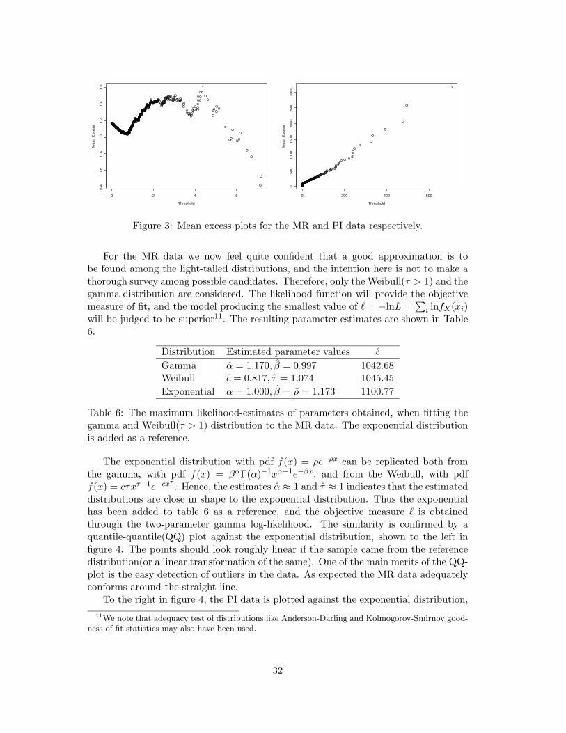
In addition to figure 1 in section 2, the characteristics are further emphasized whenplotting the empirical mean excess functions of both data sets in figure 3. The samplemean excess function is defined by

en(u) =

∑ni=1(xi − u)+∑n

i=1 1xi>u,

that is, the sum of the excesses over the threshold u divided by the number of excesses.en(u) is then plotted with u ranging between xn:n < u < x1:n where xi:n denotes the i:thorder statistic of the sample. Thus, the sample mean excess function is the empiricalestimate of the mean excess function, defined as e(u) = E[X − u | X > u], whichwe recall from section 3 as a shifted version of the CV aR risk measure. A graphicalrepresentation of the mean excess function, of some standard distributions, is given inEmbrechts et al. (1997) p.29. If the points show an upward trend, then this is a signof heavy-tailed behavior. For exponentially distributed data a horizontal line would beexpected and data from a short tailed distribution would show a downward trend.

In Hogg & Klugman (1984) p.177 a detailed flow-chart is presented, as a guide infitting loss distributions. They propose to minimize objective functions(i.e. maximumlikelihood) for different distributional models and make a first selection among themodels returning the lowest values. To make the final selection the theoretical limitedexpected value function, E[min(X, d)], is also compared to its empirical counterpart.To start with two parameter models are chosen, and in order to test these modelsagainst their three-parameter(higher order) generalizations, likelihood ratio statisticsare used.

10We are here, by making the assumption of a homogeneous poisson distribution for the loss frequency,implicitly also making the assumption that the poisson process limit law in section 5.2. is fulfilled.

31

0 2 4 6

0.4

0.6

0.8

1.0

1.2

1.4

1.6

Threshold

Mea

n E

xces

s

0 200 400 600

050

010

0015

0020

0025

0030

00

Threshold

Mea

n E

xces

s

Figure 3: Mean excess plots for the MR and PI data respectively.

For the MR data we now feel quite confident that a good approximation is tobe found among the light-tailed distributions, and the intention here is not to make athorough survey among possible candidates. Therefore, only the Weibull(τ > 1) and thegamma distribution are considered. The likelihood function will provide the objectivemeasure of fit, and the model producing the smallest value of ` = −lnL =

∑

i lnfX(xi)will be judged to be superior11. The resulting parameter estimates are shown in Table6.

Distribution Estimated parameter values `

Gamma α = 1.170, β = 0.997 1042.68Weibull c = 0.817, τ = 1.074 1045.45

Exponential α = 1.000, β = ρ = 1.173 1100.77

Table 6: The maximum likelihood-estimates of parameters obtained, when fitting thegamma and Weibull(τ > 1) distribution to the MR data. The exponential distributionis added as a reference.

The exponential distribution with pdf f(x) = ρe−ρx can be replicated both fromthe gamma, with pdf f(x) = βαΓ(α)−1xα−1e−βx, and from the Weibull, with pdff(x) = cτxτ−1e−cxτ

. Hence, the estimates α ≈ 1 and τ ≈ 1 indicates that the estimateddistributions are close in shape to the exponential distribution. Thus the exponentialhas been added to table 6 as a reference, and the objective measure ` is obtainedthrough the two-parameter gamma log-likelihood. The similarity is confirmed by aquantile-quantile(QQ) plot against the exponential distribution, shown to the left infigure 4. The points should look roughly linear if the sample came from the referencedistribution(or a linear transformation of the same). One of the main merits of the QQ-plot is the easy detection of outliers in the data. As expected the MR data adequatelyconforms around the straight line.

To the right in figure 4, the PI data is plotted against the exponential distribution,

11We note that adequacy test of distributions like Anderson-Darling and Kolmogorov-Smirnov good-ness of fit statistics may also have been used.

32

0 2 4 6 8

02

46

Ordered Data

Exp

onen

tial Q

uant

iles

0 2000 4000 6000 8000

02

46

Ordered Data

Exp

onen

tial Q

uant

iles

Figure 4: QQ-plots for motor rescue and personal injury data respectively

and the concave departure from the straight line indicates a heavier tailed distribution.We have now seen several indications of heavy-tailed behavior for the PI data. In fact,suppose that X has a GPD with parameters ξ < 1 and β, then the mean excess functionis

e(u) = E[X − u | X > u] =β + ξu

1 − ξ, β + ξu > 0.

Thus, if the empirical plot seems to follow a straight line with a positive slope above acertain value u, there is an indication of the excesses following a GPD with a positiveshape parameter.

Recall figure 3, the mean excess plot for the PI data is sufficiently straight over allvalues of u emphasizing the fit of an GPD, and it is difficult to pinpoint a superior uniquechoice from only the visual inspection of the same. The choice of threshold is a trade-off,since a value too high results in a estimation based on only a few data points, and thusgives highly variable estimates whereas a value too low gives biased estimates sincethe limit theorem may not apply. To reinforce judgement, the maximum likelihoodestimates for the shape parameter in GPDs fitted across a variety of thresholds areshown in figure 5.The shape parameter shows a relatively stable behavior, for threshold-values in thewide range approximately between 15 to 60(number of excesses ranging between 157and 60), with ξ fluctuating between 0.73 and 0.79. Within this interval, the choiceof threshold may seem somewhat arbitrary. To be more on the conservative side andincreasing the likelihood of large losses, we have chosen the threshold u = 30 givingξ = 0.7853 with standard error s.e.=0.1670. By making this final choice of threshold,we have an estimate of the excess distribution (5.3), (i.e. the conditional distributionof claims given that they exceed the threshold). Transforming the location and scaleparameters according to (5.4), we can show the fit to the whole PI data set by plottingthe estimated distribution function against the empirical distribution function, definedas Fn = n−1

∑ni=1 1xi≤x. This is done in figure 6.

Figure 6 also exhibits the last concern in the modelling of the heavy-tailed lossdistribution; how to treat the losses that falls beneath the threshold? As shown insection 4.3, the behavior of the aggregated loss is in the heavy tailed case completely

33

500 466 433 399 366 332 299 265 232 198 165 132 98 65 31

0.0

0.5

1.0

1.5

2.0

0.81 1.31 2.12 3.05 5.12 12.80 33.10 114.00

Exceedances

Sha

pe (

xi)

(CI,

p =

0.9

5)

Threshold

Figure 5: The shape parameter ξ varying with threshold u, and an asymptotic 95percent confidence band. In total 30 models are fitted.

0.1 1.0 10.0 100.0 1000.0 10000.0

0.0

0.2

0.4

0.6

0.8

1.0

x(on log scale)

Est

imat

ed d

f

Figure 6: The GPD fitted above the threshold u = 30.

34

determined by the tail of the loss distribution, and claims beneath the threshold is inthat sense of less importance. Thus for the losses under the threshold of 30, we havein the next section chosen the simplest possible estimator; the empirical distributionfunction Fn above. This is done even though, as noticed in figure 6, it shows someirregular behavior. Another reasonable non-parametric approach would be to use akernel-estimated distribution, which would smooth out these irregularities.

8.3 Stress testing and evaluation of risk measures

In the previous section, it is shown how the shape parameter in the GPD model isaffected by the choice of threshold, and this may cause a great deal of uncertainty.Inference is based on the data points in the far end tail-area of the distribution. Hence,it is also important to investigate its sensibility to the largest losses. Table 7 shows theresulting shape parameter estimate under different scenarios, such as removing/addingclaims or after assuming an over/under-estimate of the largest claim by 20 and 40percent respectively, for the chosen threshold.

Scenario Threshold(u) Excesses Shape(ξ) s.e.

Original estimate 30 107 0.785 0.170x1:n(+20%) 30 107 0.794 0.170x1:n(+40%) 30 107 0.801 0.171x1:n(-20%) 30 107 0.775 0.169x1:n(-40%) 30 107 0.761 0.169x1:n(removed) 30 106 0.634 0.161x1:n, x2:n(removed) 30 105 0.536 0.156x1:n+1(=10 000, added) 30 108 0.914 0.179

Table 7: Let xi:n denote the i:th order statistic, where x1:n = max(x1 . . . xn) is themaximum loss in the data set. Hypothetical scenarios applied to the given loss(-es) aredescribed in brackets.

Our original GPD model turns out to be robust against both over- and underesti-mates of the largest loss, with ξ ranging in a ’narrow’ interval of 0.76 to 0.80. However,we should be aware of the standard errors and, since inference is sensitive to smallchanges in the parameters, parameter uncertainty cannot be neglected. Furthermore,dropping the largest loss from the data set reduces the shape parameter estimate to0.634. Removing the next largest loss causes an even larger reduction in the estimate.If we instead introduce a new larger loss of 10000 to the data set(the previous largestbeing 7984), ξ goes up to 0.914. Hence in our case data uncertainty seems to be moreserious than both model uncertainty(in regard to choosing an appropriate threshold)and parameter uncertainty. Estimates are very sensitive to the largest observed losses,and this should be kept in mind when pooling data across banks or when introducinghypothetical shadow(i.e. expert estimates) losses to the actual loss statistics.

We now turn to the estimation of the risk measures. We start with exploring thetheoretical limit theorems of section 4.3. The VaR measure for the two cases can beobtained through direct inversion of (4.6) and (4.8) respectively. For the CVaR measure

35

we consider the integral-part in the following expression obtained through integrationby parts, with the notation from section 4.3 kept, as

E(S | S > x) = x+ E(S − x | S > x) = x+1

1 −G(x)

∫ ∞

x1 −G(t)dt. (8.2)

Asymptotic approximations are then obtained when integrating over the tail of G12.We do not intend to perform this calculation in the light-tailed case, but instead justshow the result and refer to Teugels and Willmot(1987) for details. The integral in(8.2) is given by

∫ ∞

x1 −G(t)dt ∼

eκxJ(x)

κ2(2πλL′′X(κ))1/2

[e−λ(1−LX(κ)) − e−λ], x→ ∞,

where J(x) ∼ 1. Recall from theorem 3 that κ is affected by λ = E(N) through thesolution of −λL′

X(κ) = x.In the heavy-tailed sub-exponential case we have concluded that we are in the

domain of attraction of the Frechet since 1α = ξ ≈ 0.8 > 0. Thus, we have

Gξ,β(µ)(x) =

(

1 + ξx

β

)−1/ξ

∼

(

β

ξ

)1/ξ

x−1/ξ (8.3)

with the slowly varying function C(X) = (β/ξ)1/ξ, a constant. Now, making use ofrelation (4.8), (8.2) and (8.3), we get

E(S | S > x) ∼ x+1

E(N)(1 − F (x))

∫ ∞

xE(N)(1 − F (t))dt

∼ x+1

x−αC(x)

∫ ∞

xt−αC(t)dt

= x+1

x−αC(x)x−α+1

∫ ∞

1β−αC(xβ)dβ

= x+ x

∫ ∞

1β−αC(xβ)

C(x)dβ

∼ x+ x

∫ ∞

1β−αdβ

= x+ x1

α− 1

= x(1 +1

α− 1), given α > 1.

In this case CVaR is only affected by the loss distribution, since E(N) appears as ascaling factor and hence is conditioned away.

Table 8 and 9 summarizes the values of the risk-measures, at three standard levels ofα(0.95, 0.99 and 0.999), obtained through the recursion procedure and the asymptoticformulas. To give a short recap of the input, we use the expected number of losses,

12Note the connection to the integral representation of CVaR in section 3.

36

given the three scenarios of exposure to loss in the next period. For modelling of theMR data set, a gamma loss distribution with parameters α = 1.17 and β = 1.00 ischosen. Furthermore the PI data set is modelled by the observed loss distributionwith a GPD-tail having shape ξ = 0.79, location µ = −9.39 and scale β(µ) = 10.62respectively, above the threshold of 30. Since we are modelling the loss distributionwith the empirical distribution under the threshold(i.e a mixed distribution), we areobviously restricted to the discrete panjer recursion of (6.3). When calculating theCVaR by means of the recursion procedure, the integral in (8.2) is rewritten and forthe resulting arithmetic distribution gives

∫ ∞

x1 −G(t)dt = E(S) −

∫ x

01 −G(t)dt ≈ E(S) − h

l−1∑

i=0

(1 −G(i)), (8.4)

with h denoting the span of the arithmetizised distribution, as described in section 6.2,and for simplicity chosen such that x = hl, a multiple of h.

λ V aRRec0.95 V aRApx

0.95 V aRRec0.99 V aRApx

0.99 V aRRec0.999 V aRApx

0.999

9.08 19.3 20.2 24.0 24.5 29.8 30.013.63 26.4 27.3 31.8 32.4 38.5 38.833.90 55.8 57.0 63.5 64.2 72.7 73.2

λ CV aRRec0.95 CV aRApx

0.95 CV aRRec0.99 CV aRApx

0.99 CV aRRec0.999 CV aRApx

0.999

9.08 22.3 24.0 27.0 27.6 32.9 32.713.63 29.8 32.0 34.6 36.0 41.8 41.833.90 60.7 63.5 68.4 69.2 78.2 77.2

Table 8: Risk-measures in the MR case

λ V aRRec0.95 V aRApx

0.95 V aRRec0.99 V aRApx

0.99 V aRRec0.999 V aRApx

0.999

5.14 596 491 1944 1797 11244 110798.08 897 711 2820 2573 16080 1581416.83 1722 1282 5136 4597 28740 28157

λ CV aRRec0.95 CV aRApx

0.95 CV aRRec0.99 CV aRApx

0.99 CV aRRec0.999 CV aRApx

0.999

5.14 2510 2289 8658 8371 55166 516118.08 3640 3310 12455 11987 82874 7367016.83 6712 5974 22827 21413 157081 131169

Table 9: Risk-measures in the PI case.

In the MR case the approximative formulas overestimates the VaR measure. Forα = 0.95 the difference ranges in magnitude between 2% to 5% depending on the valueof λ. When reaching the 99.9% quantile the difference is approximately 0.7%. In thePI case the approximate formulas underestimates the VaR by as much as 25% for λlarge and α = 0.95. When α = 0.999 the difference is reduced to approximately 2%,which still is a considerable deviation. As seen, these deviations are directly reflectedon the CVaR measure. We also want to point out that in the PI case the recursion

37

procedure becomes quite cumbersome and requires large arithmetic spans for α > 0.95which have an impact on the accuracy of (8.4).

8.4 Software

As for the software, the GLM function in S-Plus is used to perform the iterated re-weighted least squares in the generalized linear models. In minimization of the negativelog-likelihood function to obtain parameter estimates, the S-plus function [nlmin] whichfinds a local minimum of a nonlinear function using a general quasi-newton optimizer isused. Several functions concerning estimation techniques and exploratory data analysisin extreme value theory are available in the finMetrics module for S-plus, and the codeis left open for anyone to make modifications.

38

9 Summary and Conclusions

In the thesis we have approached the modelling of operational risk using actuarialtechniques under the assumption of independent and identically distributed data. Theultimate goal is to calculate risk measures and to this end we need to understandthe behavior of the compound loss distribution, especially in the right tail-area. Asurvey through the actuarial literature gives some theoretical background, where specialemphasis is given to the underlying individual loss distribution. A connection to causalanalysis of loss frequency is made using generalized linear models. In order to befamiliarized with the exploratory tools used in the modelling process, methods areapplied to two illustrative data-sets. Risk measures are obtained by computation of thecompound loss distribution through a recursion procedure, and furthermore comparedto asymptotic approximations. The main observations made are;

- The mathematical theory developed within the area of risk theory outlines a dis-tinction of loss distributions in two broad categories. In an operational risk con-text, the loss distributions covered by these categories will probably get us quitefar. The categories are the light-tailed distributions, with an existing momentgenerating function, and the heavy-tailed sub-exponential distributions wherethe maximum loss asymptotically determine the tail of the compound loss.

- Through GLM we have identified and linked relevant risk factors to the frequencyof losses. The poisson assumption, with partial modification for inferential pur-pose, seem plausible in this situation. For both data sets we found three significantfactors and reduced the dimension from 900 to 30 and 64 units respectively. Thissetup allows for stress-testing, and we establish three scenarios of exposure to riskwithin a future planning period of one month. The outcome is then used in theevaluation of risk-measures.

- In exploratory analysis of data sets, visual inspection of the data using variousplotting techniques, as qq-plots and empirical mean excess functions, prove to bevaluable. This is especially the case when modelling heavy-tailed data. In partic-ular, refitting series of generalized Pareto distributions and looking at the resultsgraphically is very helpful to reinforce judgement about the shape parameter.

- The MR data is very light-tailed and exponential-like distributions are well suitedto represent the data. The GPD provides a good approximation to the tail ofthe very skewed, heavy-tailed PI data. The model is in this case fairly insensitiveto choices of thresholds. Point estimates of the shape parameter faces standarderrors of a magnitude of approximately 20% of the estimate and therefore intro-duce considerable parameter uncertainty. However, the biggest problem seems tobe the data itself. By tampering with the largest losses the parameter estimatesdrastically changes, and access to reliable operational loss data therefore becomesof the outmost importance.

- When moving into the tail-area of the compound loss distribution, we need tochoose large spans in our discretization of the loss distribution to reduce the

39

computing-time in the heavy-tailed case. Depending on the desired level of accu-racy the limit theorems first becomes applicable around the 0.999 quantile. Henceother numerical methods may well be investigated to improve the computationefficiency.

The assumption of independent and identically distributed losses implies that we shouldnot be able to observe structural changes in the data over time. Looking at the timeseries plot of the PI data, we see that the three largest losses took place within a one yearperiod in the beginning of the observation-period. Embrechts et al. (2002) points outthat such irregularities of loss occurrence times are often observed in operational losstime series. To take serial dependence into account, the extension to time dependentparameters in the GPD setup is made, see further references in Embrechts et al. (1997).

In the numerical illustration, most attention is paid to the modelling of the heavy-tailed data, which is only natural. In the compound poisson case, we can use theadditive property in section 4.2, to aggregate several compound poisson variables intoa global estimate for several cells in the regulatory matrix. The heavy-tailed losseswould govern also that tail. So why should one include small losses that may be seen aspart of the running of the business? Well, the assumption about independence amonglosses is once again questionable. One could for example imagine that when an ordinarytransaction fails causing a small loss, its causes ought to be explored to remedy thesituation so that a major transaction failure does not occur. Those frequent, smalllosses may serve as a signaling device for rare but big losses. This is the key point ofthe Near-Miss approach that has been developed in the chemical, health and airlineindustries and is introduced in a operational risk context by Muermann & Oktem(2002). Such extensions obviously calls for more complex models.

40

Appendix

Model Res. DoF Deviance F-value P-value

Main effects(ME) 849 814.95

ME + A*B 829 796.32 0.82 0.70

ME + A*C 833 786.21 1.61 0.06

ME + A*D - -

ME + B*C 829 781.01 1.43 0.10

ME + B*D 824 774.67 1.38 0.10

ME + C*D 829 781.95 1.50 0.07

Table 10: The MR data: Deviance and goodness of fit-statistic in models with interac-tion.

Parameter Estimate Std.error

I -A(1) -0.54 0.36A(2) -0.43 0.14A(3) 0 0A(4) 0.37 0.09A(5) 0.19 0.10B(1) 0.05 0.17B(2) 0.02 0.14B(3) 0.05 0.12B(4) 0.06 0.10B(5) 0 0B(6) 0.05 0.11C(1) 0 0C(2) 0.21 0.09C(3) 0.63 0.10C(4) 0.70 0.16C(5) 1.13 0.14D(1) 0.40 0.11D(2) 0.20 0.11D(3) 0.24 0.11D(4) 0 0D(5) 0.39 0.16D(6) 0.40 0.12

Table 11: The MR data: Estimated relativities on log-scale in original main effectsmodel.

41

Model Res. DoF Deviance χ2-value P-value

Main effects(ME) 853 534.15

ME + A*B 833 520.52 13.63 0.85

ME + A*C 837 516.49 17.66 0.34

ME + A*D 833 511.69 22.45 0.32

ME + B*C 833 518.69 15.46 0.75

ME + B*D 828 499.45 34.70 0.09

ME + C*D 833 518.45 15.69 0.74

Table 12: The PI data: Deviance and goodness of fit-statistic in models with interac-tion.

Parameter Estimate Std.error

I -A(1) -0.07 0.34A(2) -0.35 0.16A(3) 0 0A(4) 0.11 0.10A(5) -0.05 0.11B(1) 0.91 0.16B(2) 0.13 0.16B(3) 0.35 0.14B(4) 0.43 0.13B(5) 0 0B(6) 0.02 0.14C(1) 0 0C(2) 0.01 0.09C(3) -0.20 0.13C(4) -0.17 0.23C(5) -0.28 0.25D(1) 0.37 0.12D(2) 0.32 0.12D(3) 0.07 0.14D(4) 0 0D(5) 0.42 0.18D(6) -0.06 0.16

Table 13: The PI data: Estimated relativities on log-scale in original main effectsmodel.

42

References

1. Artzner, P., Delbaen, F., Eber, J. and Heath, D. (1999): Coherent Measures ofRisk. Math. Finance 9, 3, pp. 203-228.

2. Basel Committee on Banking Supervision, Consultative Document (2001): Op-erational Risk. Available at http://www.bis.org/publ/bsbsca.htm.

3. Basel Committee on Banking Supervision, Working Paper (2001): Working Paperon the Regulatory Treatment of Operational Risk. http://www.bis.org/publ/bcbs-wp8.pdf.

4. Brockman, M.J. and Wright, T.S. (1992): Statistical Motor Rating: MakingEffective use of Your Data. J.I.A. 119, pp. 457-543.

5. Buhlmann, H. (1984): Numerical evaluation of the Compound Poisson Distribu-tion: Recursion or Fast Fourier Transform?. Scand. Actuar. J., pp. 116-126.

6. Cruz, M.G. (2002): Modeling, measuring and hedging operational risk. Wiley.

7. Daykin, C., Pentikainen, T. and Pesonen, T. (1994): Practical Risk Theory forActuaries. Chapman and Hall.

8. Delbaen, F. (1998): Coherent risk measures on general probability spaces. Work-ing paper ETH Zurich. Available at http://www.math.ethz.ch/∼delbaen.

9. Embrechts, P., Kaufmann, R. and Samorodnitsky, G. (2004): Ruin theory revis-ited: stochastic models for operational risk. Risk Management for Central BankForeign Reserves (Eds. C. Bernadell et al.) European Central Bank, FrankfurtA.M., pp.243-261.

10. Embrechts, P., Kluppelberg, C. and Mikosch, T. (1997): Modelling ExtremalEvents. Springer, New York.

11. Embrechts, P., Maejima, M. and Teugels, J. (1985): Asymptotic behavior ofCompound Distributions . Astin Bulletin 15, pp. 45-48.

12. Ebnother, S., Vanini, P., McNeil, A. and Antolinez-Fehr, P. (2001): ModellingOperational risk. Available at http://www.math.ethz.ch/∼mcneil.

13. Frachot, A., Georges, P. and Roncalli, T. (2001): Loss Distribution Approach foroperational risk. Group de Recherche Operationelle, Credit Lyonnais.

14. Frachot, A., Georges, P. and Roncalli, T. (2002): Mixing internal and externaldata for operational risk. Group de Recherche Operationelle, Credit Lyonnais.

15. Grandell, J. (1991): Aspects of Risk Theory. Springer, Berlin

16. Gut, A. (1995): An Intermediate Course in Probability. Springer.

43

17. Hogg, R. and Klugman, S. (1984): Loss Distributions. Wiley, New York.

18. Hosking J.R.M. and Wallis, J.R. (1987): Parameter and quantile estimation forthe generalized Pareto distribution. Technometrics 29, pp. 339-349.

19. Kusuoka, S. (2001): On law invariant coherent risk measures. Advances in Math-ematical Economics. Vol 3, pp.83-95.

20. McCullagh, P. and Nelder, J.A. (1983): Generalized Linear Models. Chapmanand Hall, London.

21. Muermann, A. and Oktem, U. (2002): The near-miss management to operationalrisk. Journal of Risk Finance 4,1, pp. 25-36.

22. Nystrom, K. and Skoglund, J. (2002): Quantitative Operational Risk Manage-ment. Swedbank, Group Financial Risk Control. http://www.gloriamundi.org.

23. Panjer, H.H. (1981): Recursive Evaluation of a Family of Compound Distribu-tions, Astin Bulletin, 12, pp.22-26.

24. Panjer, H.H. and Willmot, G. (1992): Insurance Risk Models. Society of Actu-aries, Schaumburg, Illinois.

25. Renshaw, A.E. (1994): Modelling the Claims Process in the Presence of Covari-ates. Astin Bulletin 24, pp. 265-285.

26. Rootzen, H. and Tajvidi, N. (1997): Extreme value statistics and wind stormlosses: a case study. Scand. Actuar. J. 1, pp. 70-94.

27. Stroter, B. (1985): The Numerical Evaluation of the Aggregate Claim Den-sity Function via Integral Equations. Blatter der Deutshe Gesellschaft fur ver-sicherungsmathematik 17, pp. 1-14.

28. Teugels, J.L. (1985): Approximation and estimation of some compound distribu-tions. Insurance: Mathematics and Economics 4, pp. 143-153.

29. Teugels, J.L. and Willmot, G. (1987): Approximations for stop-loss premiums.Insurance: Mathematics and Economics 6, pp. 195-202.

44