Linköping2010 - DiVA portal
84
Institutionen för systemteknik Department of Electrical Engineering Examensarbete Traffic Scheduling for LTE Advanced Examensarbete utfört i Communication Systems vid Tekniska högskolan i Linköping av Zhiqiang Tang LiTH-ISY-EX--10/4413--SE Linköping 2010 Department of Electrical Engineering Linköpings tekniska högskola Linköpings universitet Linköpings universitet SE-581 83 Linköping, Sweden 581 83 Linköping
Transcript of Linköping2010 - DiVA portal

Institutionen för systemteknikDepartment of Electrical Engineering
Examensarbete
Traffic Scheduling for LTE Advanced
Examensarbete utfört i Communication Systemsvid Tekniska högskolan i Linköping
av
Zhiqiang Tang
LiTH-ISY-EX--10/4413--SE
Linköping 2010
Department of Electrical Engineering Linköpings tekniska högskolaLinköpings universitet Linköpings universitetSE-581 83 Linköping, Sweden 581 83 Linköping

Traffic Scheduling for LTE Advanced
Examensarbete utfört i Communication Systemsvid Tekniska högskolan i Linköping
av
Zhiqiang Tang
LiTH-ISY-EX--10/4413--SE
Handledare: Yi Wuisy, Linköpings universitet
Examinator: Eleftherios Karipidisisy, Linköpings universitet
Linköping, 22 October, 2010

Avdelning, InstitutionDivision, Department
Division of Communication SystemsDepartment of Electrical EngineeringLinköpings universitetSE-581 83 Linköping, Sweden
DatumDate
2010-10-22
SpråkLanguage
� Svenska/Swedish� Engelska/English
�
�
RapporttypReport category
� Licentiatavhandling� Examensarbete� C-uppsats� D-uppsats� Övrig rapport�
�
URL för elektronisk versionhttp://www.commsys.isy.liu.se
http://www.ep.liu.se
ISBN—
ISRNLiTH-ISY-EX--10/4413--SE
Serietitel och serienummerTitle of series, numbering
ISSN—
TitelTitle
Trafikskedulering for LTE AdvancedTraffic Scheduling for LTE Advanced
FörfattareAuthor
Zhiqiang Tang
SammanfattningAbstract
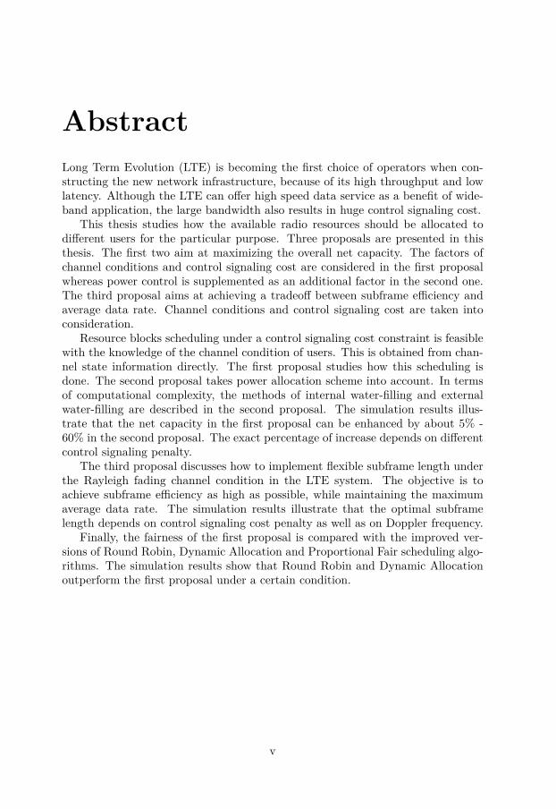
Long Term Evolution (LTE) is becoming the first choice of operators when con-structing the new network infrastructure, because of its high throughput and lowlatency. Although the LTE can offer high speed data service as a benefit of wide-band application, the large bandwidth also results in huge control signaling cost.
This thesis studies how the available radio resources should be allocated todifferent users for the particular purpose. Three proposals are presented in thisthesis. The first two aim at maximizing the overall net capacity. The factors ofchannel conditions and control signaling cost are considered in the first proposalwhereas power control is supplemented as an additional factor in the second one.The third proposal aims at achieving a tradeoff between subframe efficiency andaverage data rate. Channel conditions and control signaling cost are taken intoconsideration.
Resource blocks scheduling under a control signaling cost constraint is feasiblewith the knowledge of the channel condition of users. This is obtained from chan-nel state information directly. The first proposal studies how this scheduling isdone. The second proposal takes power allocation scheme into account. In termsof computational complexity, the methods of internal water-filling and externalwater-filling are described in the second proposal. The simulation results illus-trate that the net capacity in the first proposal can be enhanced by about 5% -60% in the second proposal. The exact percentage of increase depends on differentcontrol signaling penalty.
The third proposal discusses how to implement flexible subframe length underthe Rayleigh fading channel condition in the LTE system. The objective is toachieve subframe efficiency as high as possible, while maintaining the maximumaverage data rate. The simulation results illustrate that the optimal subframelength depends on control signaling cost penalty as well as on Doppler frequency.
Finally, the fairness of the first proposal is compared with the improved ver-sions of Round Robin, Dynamic Allocation and Proportional Fair scheduling algo-rithms. The simulation results show that Round Robin and Dynamic Allocationoutperform the first proposal under a certain condition.
NyckelordKeywords LTE, LTE Advanced, Scheduling, Control Signalling Cost

AbstractLong Term Evolution (LTE) is becoming the first choice of operators when con-structing the new network infrastructure, because of its high throughput and lowlatency. Although the LTE can offer high speed data service as a benefit of wide-band application, the large bandwidth also results in huge control signaling cost.
This thesis studies how the available radio resources should be allocated todifferent users for the particular purpose. Three proposals are presented in thisthesis. The first two aim at maximizing the overall net capacity. The factors ofchannel conditions and control signaling cost are considered in the first proposalwhereas power control is supplemented as an additional factor in the second one.The third proposal aims at achieving a tradeoff between subframe efficiency andaverage data rate. Channel conditions and control signaling cost are taken intoconsideration.
Resource blocks scheduling under a control signaling cost constraint is feasiblewith the knowledge of the channel condition of users. This is obtained from chan-nel state information directly. The first proposal studies how this scheduling isdone. The second proposal takes power allocation scheme into account. In termsof computational complexity, the methods of internal water-filling and externalwater-filling are described in the second proposal. The simulation results illus-trate that the net capacity in the first proposal can be enhanced by about 5% -60% in the second proposal. The exact percentage of increase depends on differentcontrol signaling penalty.
The third proposal discusses how to implement flexible subframe length underthe Rayleigh fading channel condition in the LTE system. The objective is toachieve subframe efficiency as high as possible, while maintaining the maximumaverage data rate. The simulation results illustrate that the optimal subframelength depends on control signaling cost penalty as well as on Doppler frequency.
Finally, the fairness of the first proposal is compared with the improved ver-sions of Round Robin, Dynamic Allocation and Proportional Fair scheduling algo-rithms. The simulation results show that Round Robin and Dynamic Allocationoutperform the first proposal under a certain condition.
v

Acknowledgments
First I would like to thank all at Communication Systems division of LinkopingUniversity, especially my supervisor Yi Wu and examiner Eleftherios Karipidis.
I also would like to thank all my friends in Sweden.
Last but not least, I would like to thank my wonderful family, for all their en-during support and always believing in me.
Zhiqiang Tang
Linkoping, Sweden, 2010
vii


Contents
1 Introduction 31.1 LOLA Project . . . . . . . . . . . . . . . . . . . . . . . . . . . . . . 41.2 Problem Statement . . . . . . . . . . . . . . . . . . . . . . . . . . . 41.3 Thesis Scope . . . . . . . . . . . . . . . . . . . . . . . . . . . . . . 51.4 Thesis Layout . . . . . . . . . . . . . . . . . . . . . . . . . . . . . . 5
2 LTE and LTE Advanced Background 72.1 LTE and LTE Advanced . . . . . . . . . . . . . . . . . . . . . . . . 72.2 LTE Protocol Architecture . . . . . . . . . . . . . . . . . . . . . . 8
2.2.1 LTE Protocol Architecture for the Downlink . . . . . . . . 82.2.2 Scheduler . . . . . . . . . . . . . . . . . . . . . . . . . . . . 10
2.3 LTE Physical Layer . . . . . . . . . . . . . . . . . . . . . . . . . . 102.3.1 Frame Structure . . . . . . . . . . . . . . . . . . . . . . . . 102.3.2 Resource Allocation for Signals . . . . . . . . . . . . . . . . 11
2.4 Multiple Access Technique for LTE/LTE Adavanced . . . . . . . . 142.4.1 OFDM . . . . . . . . . . . . . . . . . . . . . . . . . . . . . 142.4.2 OFDMA . . . . . . . . . . . . . . . . . . . . . . . . . . . . . 16
3 Scheduling Algorithms 173.1 Scheduling Algorithms Classification . . . . . . . . . . . . . . . . . 173.2 Scheduling Algorithms for Non-Real-Time Flows . . . . . . . . . . 18
3.2.1 Max Rate . . . . . . . . . . . . . . . . . . . . . . . . . . . . 183.2.2 Round Robin . . . . . . . . . . . . . . . . . . . . . . . . . . 183.2.3 Proportional Fair . . . . . . . . . . . . . . . . . . . . . . . . 19
3.3 Scheduling Algorithms for Real-Time Flows . . . . . . . . . . . . . 203.3.1 Largest Delay First . . . . . . . . . . . . . . . . . . . . . . . 203.3.2 Modified Largest Weighted Delay First . . . . . . . . . . . . 20
3.4 Scheduling Algorithms for Mixture of Real-Time and Non-Real-Time Flows . . . . . . . . . . . . . . . . . . . . . . . . . . . . . . . 213.4.1 Exponential Rule . . . . . . . . . . . . . . . . . . . . . . . . 213.4.2 Utility Function . . . . . . . . . . . . . . . . . . . . . . . . 21
ix
x Contents
4 Scheduling Under a Control Signaling Cost Constraint 234.1 Background . . . . . . . . . . . . . . . . . . . . . . . . . . . . . . . 234.2 Proposed Scheduling Algorithm Under a Control Signaling Cost
Constraint for LTE/LTE Advanced . . . . . . . . . . . . . . . . . . 244.2.1 Notation . . . . . . . . . . . . . . . . . . . . . . . . . . . . . 244.2.2 Individual Transmission of Scheduling Maps{Mk} . . . . . 254.2.3 Broadcasting of Joint Scheduling Map M . . . . . . . . . . 274.2.4 Optimal Assignment S Given the User Set U . . . . . . . . 294.2.5 Selecting the Set of Active Users U . . . . . . . . . . . . . . 29
4.3 Power Optimization . . . . . . . . . . . . . . . . . . . . . . . . . . 304.3.1 Water-filling . . . . . . . . . . . . . . . . . . . . . . . . . . 304.3.2 External Water-filling . . . . . . . . . . . . . . . . . . . . . 314.3.3 Internal Water-filling . . . . . . . . . . . . . . . . . . . . . . 32
4.4 Simulation Results . . . . . . . . . . . . . . . . . . . . . . . . . . . 334.4.1 Individual and Broadcast Scheduling Map Transmission . . 334.4.2 External Water-filling . . . . . . . . . . . . . . . . . . . . . 364.4.3 Internal Water-filling . . . . . . . . . . . . . . . . . . . . . . 40
5 Adaptive Length Subframe 455.1 Rayleigh Fading Channel . . . . . . . . . . . . . . . . . . . . . . . 455.2 Proposed Scheduling Algorithm of Adaptive Length Subframe for
LTE Advanced . . . . . . . . . . . . . . . . . . . . . . . . . . . . . 485.2.1 Motivation . . . . . . . . . . . . . . . . . . . . . . . . . . . 485.2.2 Subframe Length Optimization Algorithm . . . . . . . . . . 49
5.3 Simulation Results . . . . . . . . . . . . . . . . . . . . . . . . . . . 505.3.1 Optimal Subframe Length for Individual and Broadcast Schedul-
ing Map Transmission Modes . . . . . . . . . . . . . . . . . 505.3.2 Influence of Different Control Signaling Cost Penalties to
Adaptive Subframe Length . . . . . . . . . . . . . . . . . . 525.3.3 Influence of Doppler Frequency to Adaptive Subframe Length 55
6 Fairness Evaluation 596.1 Proportional Fair . . . . . . . . . . . . . . . . . . . . . . . . . . . . 59
6.1.1 Notation . . . . . . . . . . . . . . . . . . . . . . . . . . . . . 606.1.2 Proportional Fair Under a Control Signaling Cost Constraint 60
6.2 Dynamic Allocation . . . . . . . . . . . . . . . . . . . . . . . . . . 616.3 Round Robin . . . . . . . . . . . . . . . . . . . . . . . . . . . . . . 626.4 Simulation Results . . . . . . . . . . . . . . . . . . . . . . . . . . . 62
7 Conclusion 65
8 Future Work 67
Bibliography 69
Abbreviations2G Second Generation Mobile Telecommunication3G Third Generation Mobile Telecommunication3GPP 3rd Generation Partnership ProjectARQ Automatic Repeat-reQuestAWGN Additive White Gaussian NoiseCA Carrier AggregationCP Cyclic PrefixCSI Channel State InformationDCI Downlink Control InformationDSCH Downlink Shard ChannelDSL Digital Subscriber LineDTCH Dedicated Traffic ChannelETSI European Telecommunications Standards InstituteFDMA Frequency Division Multiple Accessi.i.d. Independent and Identically DistributedLOLA Low Latency in Wireless CommunicationLTE Long Term EvolutionMAC Medium Access ControlMBSFN Multicast/Broadcast over Single Frequency NetworkM2M Machine to MachineNRT Non-Real-TimeOFDM Orthogonal Frequency Division MultiplexingOFDMA Orthogonal Frequency Division Multiple AccessPCFICH Physical Control Format Indicator ChannelPDCCH Physical Downlink Control ChannelPDU Protocol Data UnitPHICH Physical Hybrid ARQ Indicator ChannelPHY Physical LayerPRB Physical Resource BlockQoS Quality of ServiceRLC Radio Link ControlRNTI Radio Network Temporary IdentifierRRC Radio Resource ControlRT Real-TimeSAE System Architecture EvolutionSB Schedule BlockSDU Service Data UnitTTI Transmission Time IntervalWiMAX Worldwide Interoperability for Microwave Access


Chapter 1
Introduction
Due to the development of electronic and information technology, telecommuni-cation industry has been undergoing rapid growth. In 1991, the Finnish operatorRadiolinjia launched the first 2G network in the world, which was built for voiceservice and low data transmission [3]. Ten years later, the first pre-commercial 3Gnetwork was launched by the Japanese operator NTT DoCoMo [4]. Besides lowdata transmission services, such as instance fax and conventional voice services,video and multimedia services are also supported by 3G network, as the result ofits data transfer rate which can be as high as 2Mbit.
In recent years, some data services, such as mobile TV, file sharing, locationbased services and social networking have grown very fast. Faster upload anddownload speeds are expected by the end users. As a 3.9G technology, Long TermEvolution (LTE) is proposed by 3rd Generation Partnership Project (3GPP) tomeet these requirements. On December 14, 2009, the first commercial LTE wasdeployed in Scandinavian countries by the Swedish-Finnish operator TeliaSonera.The Stockholm survey shows that the throughput is up to 42.8Mbit per secondfor downlink and 5.3 Mbit per second for uplink with 10 MHz spectral bandwidth[5].
According to a report of the US research organization Maravedis, the invest-ment of the top 25 operators which have committed to LTE for LTE infrastructurecould amount to 14 billion dollars by 2015. At that time, these operators will pro-vide commercial LTE service for more than 226 million subscribers [23].
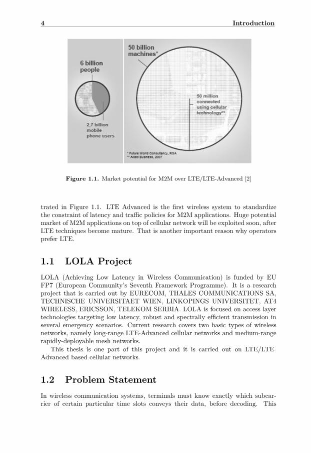
There are several reasons why operators prefer LTE. One is that the higherbandwidth speed and the higher system capacity of LTE attract operators. Band-width is not the bottleneck for high data rate services any more. Furthermore,the latency of end to end in LTE is possible to be kept within 50 ms and it makeswireless access comparable to Digital Subscriber Line (DSL). From operators’ per-spective, it means that there are several strategic low-latency application areassupported by LTE with respect to revenue potential [6]. Take Machine to Ma-chine (M2M) applications for example. Comparing to 2.7 billion mobile phoneusers out of 6 billion people, there are 50 billion machines in the world, and only50 million of them are connected to networks with cellular technology, as illus-
3
4 Introduction
Figure 1.1. Market potential for M2M over LTE/LTE-Advanced [2]
trated in Figure 1.1. LTE Advanced is the first wireless system to standardizethe constraint of latency and traffic policies for M2M applications. Huge potentialmarket of M2M applications on top of cellular network will be exploited soon, afterLTE techniques become mature. That is another important reason why operatorsprefer LTE.
1.1 LOLA ProjectLOLA (Achieving Low Latency in Wireless Communication) is funded by EUFP7 (European Community’s Seventh Framework Programme). It is a researchproject that is carried out by EURECOM, THALES COMMUNICATIONS SA,TECHNISCHE UNIVERSITAET WIEN, LINKOPINGS UNIVERSITET, AT4WIRELESS, ERICSSON, TELEKOM SERBIA. LOLA is focused on access layertechnologies targeting low latency, robust and spectrally efficient transmission inseveral emergency scenarios. Current research covers two basic types of wirelessnetworks, namely long-range LTE-Advanced cellular networks and medium-rangerapidly-deployable mesh networks.
This thesis is one part of this project and it is carried out on LTE/LTE-Advanced based cellular networks.
1.2 Problem StatementIn wireless communication systems, terminals must know exactly which subcar-rier of certain particular time slots conveys their data, before decoding. This
1.3 Thesis Scope 5
information is packaged into scheduling maps. The scheduling maps are sent tothe terminals by control signaling. The overhead caused by control signaling issignificant in LTE/LTE Advanced due to the huge bandwidth.
In LTE/LTE Advanced, resource block is the minimum resource unit and sub-frame is the minimum time slot that can be allocated by scheduler. The LTE/LTEAdvanced systems with 20MHz channel bandwidth have 100 resource blocks. As-sume 10 terminals are scheduled in one subframe in the case of downlink schedul-ing. It needs at least 100 × 10 = 1000 bits per subframe for scheduling map inindividual transmission mode to inform terminals about the allocation of resourceblocks. As a result, about 1 Mbit throughput per second is used for control sig-naling overhead. It is necessary to find a good solution to reduce overhead causedby scheduling maps while keeping flexibility of resource blocks allocation.
Although resource allocation types 0, 1, 2 are specified by 3GPP release 8 [1] tomitigate control signaling overhead, each type has its drawbacks. In other words,they do not perform as well as 3GPP expected. This thesis will analyze threetypes of solutions proposed recently and come up with new algorithms to alleviatethe influence of control signaling overhead on the overall system performance.
1.3 Thesis ScopeThe research on control signaling overhead and scheduling in this thesis is onlyfor the downlink of LTE/LTE Advanced system. Since this project is at its pri-mary stage, all the scenarios are using traditional single antenna transmitter andreceiver.
1.4 Thesis LayoutChapter 1 gives a short introduction to LOLA of which this thesis is a part. Af-ter analyzing why LTE/LTE Advanced probably will become the most popularcommunication system in the world, this chapter points out the control signalingoverhead problem that LTE/LTE Advanced is suffering from.
Chapter 2 introduces the technical background of LTE and LTE Advanced. Fur-thermore, the radio interface architecture of LTE, specifically the physical layer ispresented.
Chapter 3 states several classic scheduling algorithms for Real-Time (RT) andNon-Real-Time (NRT) flows.
Chapter 4 analyzes recent research on lightening the influence of signaling over-head on the overall system performance for wideband communication systems. Italso demonstrates two proposed scheduling algorithms under a control signalingcost constraint for LTE/LTE Advanced.

6 Introduction
Chapter 5 presents a novel adaptive subframe scheduling algorithm on the ba-sis of Chapter 4, which brings up a novel hypothesis beyond 3GPP LTE standard.
Chapter 6 evaluates the fairness of the proposed algorithms by comparing it withsome reference algorithms.
Chapter 7 summarizes the research findings of Chapter 4, 5 and 6.
Chapter 8 describes some issues left by this thesis. Hopefully, future work willsolve these problems.
Chapter 2
LTE and LTE AdvancedBackground
2.1 LTE and LTE AdvancedAs the minor update of Release 9 of current LTE specification, LTE Advanced willbe coincident with LTE Release 10. The work on LTE Advanced standard like IMTAdvanced is ongoing. The LTE Advanced finalization in 3GPP is expected to beaccomplished in 2011, aligning with finalization of IMT Advanced in ITU.
The LTE Advanced can achieve much better system performance than LTE. Itsupports for peak data up to 1Gbps in the downlink and 500 Mbps in the uplink,in contrast with 100Mbps in the downlink and 50 Mbps in the uplink of LTE. Inaddition to substantial improvement for cells and terminals, the LTE Advancedprovides not only more efficient spectrum utilization, but also the higher powerefficiency for both infrastructure and terminals.
To carry out above key performance, the following potential technology com-ponents of LTE Advanced are introduced.
• Wider bandwidth and carrier aggregationIn order to fulfil the higher peak data rate, Carrier Aggregation (CA) isintroduced to obtain wider bandwidth. Instead of adjacent component car-riers, non adjacent component carriers are supported by CA for the LTEAdvanced.
• Extended multi antenna transmissionSupport for spatial multiplexing on the uplink and extension of spatial mul-tiplexing on the downlink are expected in the LTE Advanced.
• Advanced repeaters and relay networks [13]Allowing for cost of network infrastructure, relays are proposed in the LTEAdvanced to extend cell coverage and increase data rate. The relay is inter-mediate post between eNodeB and terminals for cell edge.
7
8 LTE and LTE Advanced Background
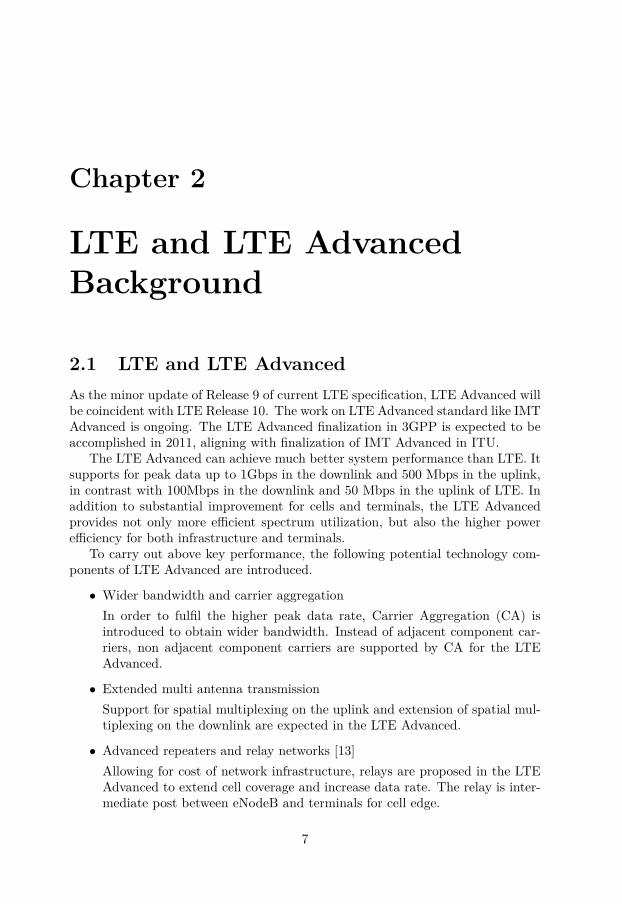
Figure 2.1. LTE protocol architecture for the downlink [11]
2.2 LTE Protocol ArchitectureThe protocol architecture is a little different between the downlink and the up-link. This thesis is focused on the downlink scheduling, so only LTE radio interfacearchitecture for the downlink is introduced. The overview of LTE protocol archi-tecture is shown in Figure 2.1.
2.2.1 LTE Protocol Architecture for the Downlink• RRC layerRadio Resource Control (RRC) handles control plane signaling. In additionto security and Quality of Service (QoS) management, RRC is in chargeof establishment, maintenance, releasing of RRC connection and mobilitymanagement.
• PDCP layerCore network sends data to eNodeB in the form of IP packets. In order toreduce the number of bits transmitted in radio interface, eNodeB uses Pack-age Data Convergence Protocol (PDCP) to compress IP header and cipherthe transmitted data at the transmitters side. At the receivers side, PDCPperforms decompression and deciphering corresponding to transmitters.

2.2 LTE Protocol Architecture 9
Figure 2.2. Physical channel, transport channel and logical channel
• RLC layer
Data is transmitted to Radio Link Control (RLC) Service Data Unit (SDU)buffer from PDCP layer. RLC is responsible for segmentation or concate-nating data selected from SDU buffer and creating the RLC Protocol DataUnit (PDU), according to scheduler’s command. In addition, retransmissionmechanism is supported by RLC to assure delivering error free data to upperlevel.
• MAC layer
Medium Access Control (MAC) offers service to RLC in the form of logicalchannels. It is shown in Figure 2.2. Several types’ logical channels are definedin MAC for different types of information carried by RLC. In general, logicalchannels are classified into control channels and traffic channels. Control andconfiguration information is transmitted via control channels and terminals’data is transmitted via traffic channels. Furthermore, MAC deals with logicalchannel multiplexing for the purpose of making full use of resources andhandles hybrid Automatic Repeat-reQuest (ARQ) retransmission. Uplinkand downlink scheduling is supported by MAC as well. It will be particularlyintroduced in Section 2.2.2.
• Physical layer
Physical layer (PHY) offers service to MAC in the form of transport channels.There are certain rules on how to map the logical channels to transportchannels regarding of types of information. Mapping of the logical channelsto transport channels is implemented in MAC, by following above rules.The PHY is used to handle coding/decoding, modulation/demodulation,multi antenna mapping and other typical physical layer functions. Finally,the signals are mapped to physical channels and transmitted over the radiointerface.
10 LTE and LTE Advanced Background
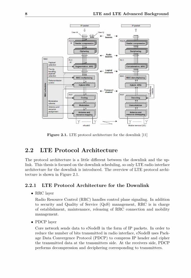
Figure 2.3. LTE frame structure and physical resource [11]
2.2.2 SchedulerThe scheduler is in the MAC layer, but it controls MAC layer and Physical layerat the same time. Scheduler can be divided into downlink scheduler for downlinkscheduling and uplink scheduler for uplink scheduling.
• Downlink schedulerThe eNodeB periodically receives Channel State Information (CSI) reports,which are the feedback from terminal to report the downlink channel condi-tions. For channel-dependent scheduling, downlink scheduler takes channelstate, buffer status and priorities into account. Then it decides resourceblocks allocation, the modulation scheme, and antenna mapping for termi-nals. As a result, downlink scheduler decision controls RLC segmentation,MAC multiplexing and Hybrid ARQ, PHY channel coding, PHY modulationand antenna mapping.
• Uplink schedulerSimilar to downlink, eNodeB uplink scheduler decides resource blocks allo-cation. However, logical channel multiplexing is controlled by terminals andchannel state estimation is done for channel-dependent scheduling by eN-odeB with reference signals transmitted from each terminal covered by thiseNodeB. With the knowledge of channel conditions, uplink scheduler makesdecisions to control channel coding and modulation scheme of terminals.
2.3 LTE Physical Layer2.3.1 Frame StructureThe LTE frame structure is illustrated in Figure 2.3. Each LTE frame is 10milliseconds in duration. It consists of ten subframes of length 1 millisecond with

2.3 LTE Physical Layer 11
Figure 2.4. Resource block [11]
equal size. Two slots of equal size constitute a subframe. Each slot consists ofseveral Orthogonal Frequency Division Multiplexing (OFDM) symbols includingcyclic prefix.
In LTE, Physical Resource Block (PRB) is the minimum resource unit thatcan be allocated by scheduler. In contrast with 48 subcarriers per slot in WiMAX,PRB consists of 12 consecutive subcarriers for one slot in duration [17] and oneslot is constituted by seven or six symbols depending on the cyclic prefix length(normal or extended), seen in Figure 2.4.
2.3.2 Resource Allocation for SignalsThe subframe is divided into control region and data region. Control signalingis allocated to the control region. Terminals’ data and uplink control signalingare allocated to data region. Reference signals are allocated to control region anddata region. The size of control region can be adjusted according to the amount ofcontrol signaling which is used to maintain communication between eNodeB andterminals, more specifically one, two, or three symbols.
2.3.2.1 Downlink Reference Signals
The eNodeB inserts reference symbols that are known by the receivers and thetransmitters into resource blocks with a constant power so that terminals canestimate instantaneous downlink channel conditions. Information about instanta-neous downlink channel conditions that can be used for coherent demodulation isreported to eNodeB for scheduling.
• Cell specific downlink reference signals
12 LTE and LTE Advanced Background
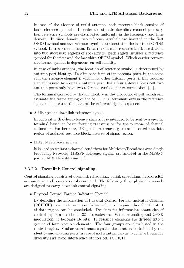
In case of the absence of multi antenna, each resource block consists offour reference symbols. In order to estimate downlink channel precisely,four reference symbols are distributed uniformly in the frequency and timedomain. In time domain, two reference symbols are inserted in the firstOFDM symbol and two reference symbols are located in the last third OFDMsymbol. In frequency domain, 12 carriers of each resource block are dividedinto two successive regions of six carriers. Each region includes a referencesymbol for the first and the last third OFDM symbol. Which carrier conveysa reference symbol is dependent on cell identity.In case of multi antenna, the location of reference symbol is determined byantenna port identity. To eliminate from other antenna ports in the samecell, the resource element is vacant for other antenna ports, if this resourceelement is used by a certain antenna port. For a four antenna ports cell, twoantenna ports only have two reference symbols per resource block [11].The terminal can receive the cell identity in the procedure of cell search andestimate the frame timing of the cell. Thus, terminals obtain the referencesignal sequence and the start of the reference signal sequence.
• A UE specific downlink reference signalsIn contrast with other reference signals, it is intended to be sent to a specificterminal based on beam forming transmission for the purpose of channelestimation. Furthermore, UE specific reference signals are inserted into dataregion of assigned resource block, instead of signal region.
• MBSFN reference signalsIt is used to estimate channel conditions for Multicast/Broadcast over SingleFrequency Network. MBSFN reference signals are inserted in the MBSFNpart of MBSFN subframe [11].
2.3.2.2 Downlink Control signaling
Control signaling consists of downlink scheduling, uplink scheduling, hybrid ARQacknowledge and power control command. The following three physical channelsare designed to carry downlink control signaling.
• Physical Control Format Indicator ChannelBy decoding the information of Physical Control Format Indicator Channel(PCFICH), terminals can know the size of control region, therefore the startof data region can be concluded. Two bits for information about size ofcontrol region are coded in 32 bits codeword. With scrambling and QPSKmodulation, it becomes 16 bits. 16 resource elements are divided into 4groups of four resource elements. The four groups are distributed in thecontrol region. Similar to reference signals, the location is decided by cellidentity and antenna ports in case of multi antenna so as to achieve frequencydiversity and avoid interference of inter cell PCFICH.
2.3 LTE Physical Layer 13
Type 0
Type Bitmap
Type 1
Type Subset L/R Bitmap
Type 2
Start Length
Figure 2.5. Resource allocation type 0, 1 and 2
• Physical Hybrid ARQ Indicator ChannelIt is used to response uplink UL-SCH transmission with Hybrid ARQ ac-knowledgement. The Physical Hybrid ARQ Indicator Channel (PHICH)are mapped to resource elements in the first symbol of control region, afterfinishing PCFICH allocation.
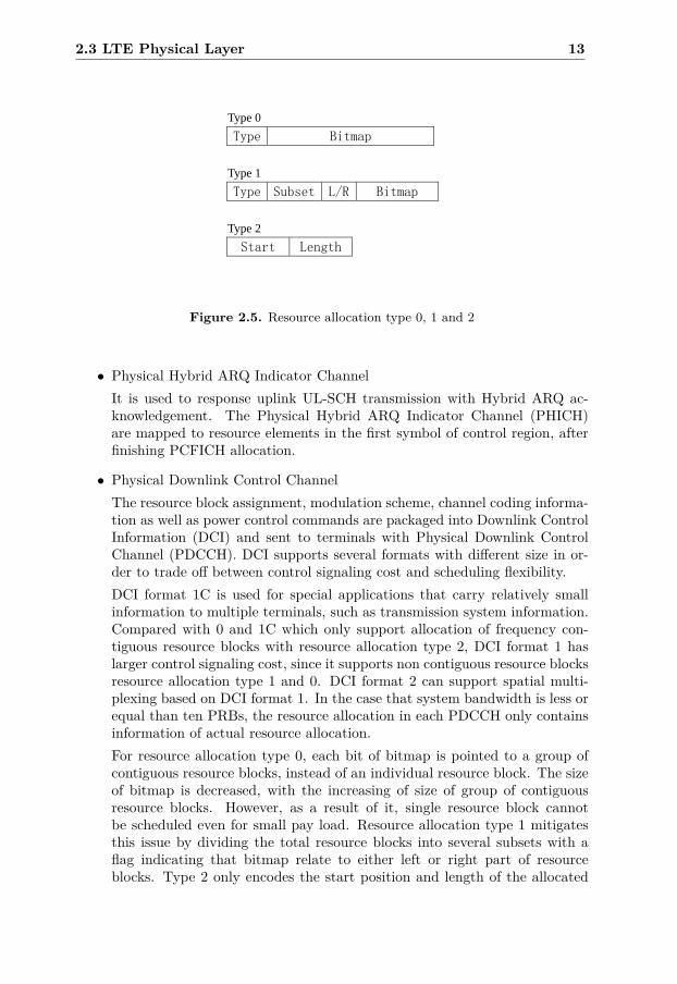
• Physical Downlink Control ChannelThe resource block assignment, modulation scheme, channel coding informa-tion as well as power control commands are packaged into Downlink ControlInformation (DCI) and sent to terminals with Physical Downlink ControlChannel (PDCCH). DCI supports several formats with different size in or-der to trade off between control signaling cost and scheduling flexibility.DCI format 1C is used for special applications that carry relatively smallinformation to multiple terminals, such as transmission system information.Compared with 0 and 1C which only support allocation of frequency con-tiguous resource blocks with resource allocation type 2, DCI format 1 haslarger control signaling cost, since it supports non contiguous resource blocksresource allocation type 1 and 0. DCI format 2 can support spatial multi-plexing based on DCI format 1. In the case that system bandwidth is less orequal than ten PRBs, the resource allocation in each PDCCH only containsinformation of actual resource allocation.For resource allocation type 0, each bit of bitmap is pointed to a group ofcontiguous resource blocks, instead of an individual resource block. The sizeof bitmap is decreased, with the increasing of size of group of contiguousresource blocks. However, as a result of it, single resource block cannotbe scheduled even for small pay load. Resource allocation type 1 mitigatesthis issue by dividing the total resource blocks into several subsets with aflag indicating that bitmap relate to either left or right part of resourceblocks. Type 2 only encodes the start position and length of the allocated

14 LTE and LTE Advanced Background
Figure 2.6. Overlapping spectrum of an OFDM signal
resource block. The illustration of resource block allocation types is shownin Figure 2.5. Although these resource allocation types mitigate the cost ofcontrol signaling, they are still not optimal. One of the main objectives ofthis thesis is to further reduce control signaling cost yielded by DownlinkControl Channel, thus to improve system performance. More detail will bediscussed in Section 3.2, 3.3 and 3.4.In this thesis, control signaling overhead only considers delivery schedulingmap cost of Downlink Control Channel due to its large throughput, comparedwith other control signaling cost generated by PCFIC and PHICH.
2.4 Multiple Access Technique for LTE/LTE Ada-vanced
2.4.1 OFDMOFDM is a popular scheme for wideband digital communication, applied in LTE/LTE Advanced network. Its advantage lies in dealing with frequency selectivefading and intersymbol interference with high spectral efficiency, whereas its dis-advantage is high peak to average power ratio as well as sensitivity to Dopplershift and to frequency synchronization.
2.4.1.1 OFDM Principle
The basic idea of OFDM is breaking available bandwidth into several sub-carriers.Based on the fundamental idea that several slow speed streams in parallel areequal to one high speed stream, the data stream is divided into several small datastreams. Each small data stream is mapped to one sub-carrier and modulated bydigital modulation scheme, such as QAM, QPSK.
From the perspective of frequency, OFDM has high spectral efficiency. Eachsub-carrier is closer to each other without guard band, as sub-carriers are orthog-onal. In other words, the peak of one sub-carrier is intersecting with the null of

2.4 Multiple Access Technique for LTE/LTE Adavanced 15
Figure 2.7. OFDM symbol structure [19]
Figure 2.8. OFDMA VS OFDM [31]
neighbour sub-carriers, as illustrated in Figure 2.6. Therefore, OFDM is one ofthe most efficient spectrum modulation in wideband wireless communication.
2.4.1.2 Cyclic Prefix
Under the principle of OFDM, high speed data stream is divided into several lowerspeed narrow band streams. The advantage of longer duration of lower speedstreams is utilized for eliminating Inter Symbol Interference (ISI), since symbolduration of lower speed streams is much larger than the maximum delay spreadin general.
In wireless telecommunication, transmission suffers multipath. Multipath causeslost of orthogonality between sub-carriers. Meanwhile lost of orthogonality be-tween sub-carriers can result in Inter Carrier Interference (ICI). In order to over-come ICI, the cyclic code is introduced to relieve issue in Figure 2.7. The contentof OFDM information consists of cyclic prefix and OFDM symbol. The cyclicprefix is a copy of the end part of OFDM symbol. It plays two roles here. Oneof them is to convert linear convolution into circular convolution in order to keepsub-carriers orthogonal in multipath conditions. The other is to prevent ISI as aguard space between successive symbols. On one hand, the period of cyclic prefixshould be selected as long as anticipated degree of delay spread at least for over-coming ICI/ISI. On the other hand, the period of cyclic prefix should be limited,because it reduces the data rate up to R((T − Tcp)/T ).

16 LTE and LTE Advanced Background
Figure 2.9. OFDMA model [16]
2.4.2 OFDMAOrthogonal Frequency Division Multiple Access (OFDMA) is a combination ofOFDM and FDMA. OFDM assigns all sub-carriers to one terminal in a symbol inthe time domain (see Figure 2.8). In OFDMA, sub-carriers are divided into groupsnamed sub-channels. Next, OFDMA assigns sub-channels with proper power todifferent terminals based on channel knowledge from CSI intending to maximizethe system throughput, seen in Figure 2.9.
Chapter 3
Scheduling Algorithms
The key to achieve optimal performance of base station is dynamically schedulinglimited resources like power and bandwidth to offer the best service for termi-nals with the lowest cost. For scheduling based on OFDMA, it balances maximumthroughput and fairness by scheduling time slots, sub-channels, modulation schemeand power with frequency diversity and multiuser diversity. Frequency diversityis done by utilizing the fact that each sub-channel suffers different attenuation indifferent time and frequency, due to shadowing, fast fading, multipath and so on.In a similar way, multiuser diversity is obtained by opportunistic user scheduling,since different users locate different places leading to different channel gains of anidentical sub-channel for different users. By analyzing CSI, base station recog-nizes variation of time, frequency, space and adjusts scheduling to keep optimalperformance.
In order to follow variation of channel conditions, scheduling should be donewithin the coherent time, so it requires that allocation algorithms must be fast,especially time varying channel. As mentioned in Section 2.3.1, PRB is formedfrom 12 consecutive sub-carriers in the frequency domain and seven or six consec-utive symbols in the time domain. The smallest resource unit which is allowed tobe assigned to one terminal is Schedule Block (SB) constituted by two successivePRBs. The fastest scheduling is required to be done within 1ms according to thesymbol length of SB. After scheduling, scheduling map will be sent to all termi-nals. Individual terminal only decodes received data in certain particular time andfrequency based on scheduling map.
3.1 Scheduling Algorithms ClassificationGenerally, scheduling can be divided into two classes: channel-independent schedul-ing and channel-dependent scheduling. Channel-independent scheduling does nottake channel conditions into account. Therefore the performance of this kind ofscheduling can never be optimal. On the contrary, channel-dependent schedulingcan achieve better performance by allocating resources based on channel conditionswith optimal algorithms. The following discussion about scheduling will focus on
17

18 Scheduling Algorithms
channel-dependent scheduling.Furthermore scheduling can be classified in the light of application scenarios,
since the performance of scheduling algorithms highly relies on the type of incomingflows. In order to implement maximum performance of system, it is important toselect suitable algorithms according to flows, in term of applications. The flowscan be divided into Real-Time flows, Non-Real-Time flows and mixture of Real-Time as well as Non-Real-Time flows due to the consideration of main services ofLTE, including voice service, data service, and live video service [22].
3.2 Scheduling Algorithms for Non-Real-Time FlowsThe problem of scheduling for Non-Real-Time flows can be considered as a con-cave optimization problem with utility functions on the basis of Proportional Fairalgorithm, which will be presented later. The optimization problem can be statedas objective function and constraints in mathematics [7]. Objective function ismaximizing utility function. Constraints are limitations of bandwidth and power.Scheduler pursues the optimal or suboptimal solution of above functions, whiletakes computation overhead into account.
The most popular scheduling algorithms for Non-Real-Time flows are Max-Rate, Round Robin, and Proportional Fair. The performance of Non-Real-Timealgorithms is measured with throughput and fairness.
3.2.1 Max RateAs a channel dependant scheduling, Max Rate takes advantage of multiuser di-versity to carry out maximum system throughput. First, scheduler analyzes CSIfrom terminals to obtain data rate of an identical sub-channel for different termi-nals. Then scheduler assigns this sub-channel to the terminal which can achievethe highest data rate in this sub-channel based on SNR. The Max Rate can bedescribed as
i = arg maxk
Rk,n(t)
Rk,n(t) is the data rate of terminal k for one sub-channel n in time slot t. Max-Rate algorithm causes starving terminals while it obtains maximum throughout.Terminals in bad channel conditions are never considered by scheduler, so it is nota fair algorithm. However, it can be considered as a good reference to measuretotal throughput. In Section 4.4, Max Rate is referred in order to compare withour algorithms.
3.2.2 Round RobinRound Robin is one of the simplest resources scheduling algorithms. It is com-monly applied in operating systems and computer networks. In the beginning,terminals are ordered randomly in a queue. The new terminals are inserted atthe end of the queue. The first terminal of this queue is assigned all the availableresources by scheduler, and then put it at the rear of the queue. The rest of steps

3.2 Scheduling Algorithms for Non-Real-Time Flows 19
Assign resource block according to
priority and update all users’_
kR
All resources are
assigned || All users’
requirements are satisfied
Yes
Calculate priority based on priority
function
Timer is out. Next time
slot for scheduling
No
Figure 3.1. Proportional Fair
follow the same way, until no terminal applies for resources. On one hand, it isa fair scheduling, since every terminal is given the same amount of resources. Onthe other hand, it neglects the fact that terminals in bad channel conditions needmore resources to carry out the same rate, so it is not absolutely fair. However, itis much fairer than Max Rate. Although Round Robin gives every terminal equalchance to obtain resources, the overall throughput is much lower than Max Rate,because scheduler does not consider channel conditions.
In LTE, different terminals have different service with different QoS require-ments. It is impossible to allow every terminal to take up the same resources inthe same possibility, because it will decrease efficiency of resources. Nevertheless,Round Robin is a good reference to measure the fairness of scheduling for LTE,as we did in Chapter 6.
3.2.3 Proportional FairProportional Fair is a compromise between Maximum Rate and Round Robin[27]. It pursues the maximum rate, and meanwhile assure that none of terminalsis starving. The terminals are ranked according to the priority function. Thenscheduler assigns resources to terminal with highest priority. Repeat the lasttwo steps until all the resources are used up or all the resources requirements ofterminals are satisfied. It is shown in Figure 3.1. The priority function is following
i = arg maxk
Rk,n(m)Rk(m)
Rk,n(m) is the estimation of supported data rate of terminal k for the resourceblock n. Rk(m) is the average data rate of terminal k over a windows in the past.

20 Scheduling Algorithms
TPF is the windows size of average throughput and can be adjusted to maintainfairness. Normally TPF should be limited in a reasonable range so that terminalscannot notice the quality variation of the channels.
Rk(m+ 1) ={
(1− 1TPF
)Rk(m) + 1TPF
Rk,n(m), if user k is selected(1− 1
TPF)Rk(m), if user k is not selected
In LTE, two strategies are considered for Rk update. The one is that Rk is updatedafter all resource blocks are allocated. The other is that Rk is updated after eachresource block allocation. Because of its better performance [26], this thesis onlyintroduces the second one, which also will be used in Chapter 6 as a referencealgorithm.
3.3 Scheduling Algorithms for Real-Time FlowsReal-Time flows have more strict delay restraint than Non-Real-Time flows result-ing in the reduction of influence of error correction. In wireless communication,Real-Time flows can be modeled as arrival process of independent packets to re-spective queues, under a delay target constraint. For different wireless networkmodels, there are several stabilizing policies to satisfy different delay target con-straints [22]. For example, the stabilizing policy of system whose delay target isthe maximum delay deadline is to make sure that the length of queues is in acertain bound.
The most popular scheduling algorithms for Real-Time flows are Largest DelayFirst, Modified Largest Weighted Delay First. Delay experience, packet loss rateand fairness are main performance metrics for Real-Time flows.
3.3.1 Largest Delay FirstThe first package received by base station will be sent out in the first place.
i = arg maxk
Wk(t)
Wk(t) is the time that package of terminal k has spent at the base station waitingfor scheduling [24]. Similar to Round Robin, neglecting channel conditions leadsto poor throughput. Even so, it is still a good reference for delay experienceevaluation.
3.3.2 Modified Largest Weighted Delay FirstMLWDF attempts to balance the weighted delays of packets, while tries to makeuse of channel resource efficiently. In the mathematic expression, the delay pos-sibility should satisfy Pr{Wk > τk} ≤ ρk and the requirement of throughput isRk > rk. The definition of Wk(t) is the same as Largest Delay First and τk isthe threshold of delay for terminal k. ρk is the maximum allowable possibility ofexceeding τk. Rk is average throughput of terminal k. rk is a predefined minimum
3.4 Scheduling Algorithms for Mixture of Real-Time and Non-Real-Time Flows 21
throughput for terminal k. In each time slot t, terminal i is selected according tofollowing priority function.
i = arg maxk
γkRk(t)Wk(t)
Where delay factor γk = akRk(t)
is an arbitrary constant. ak is characterizing thedesired QOS for terminal k [8].
Although this thesis has not had enough time to extend our algorithms forReal-Time applications, MLWDF are studied here to prepare for the future workin Chapter 8.
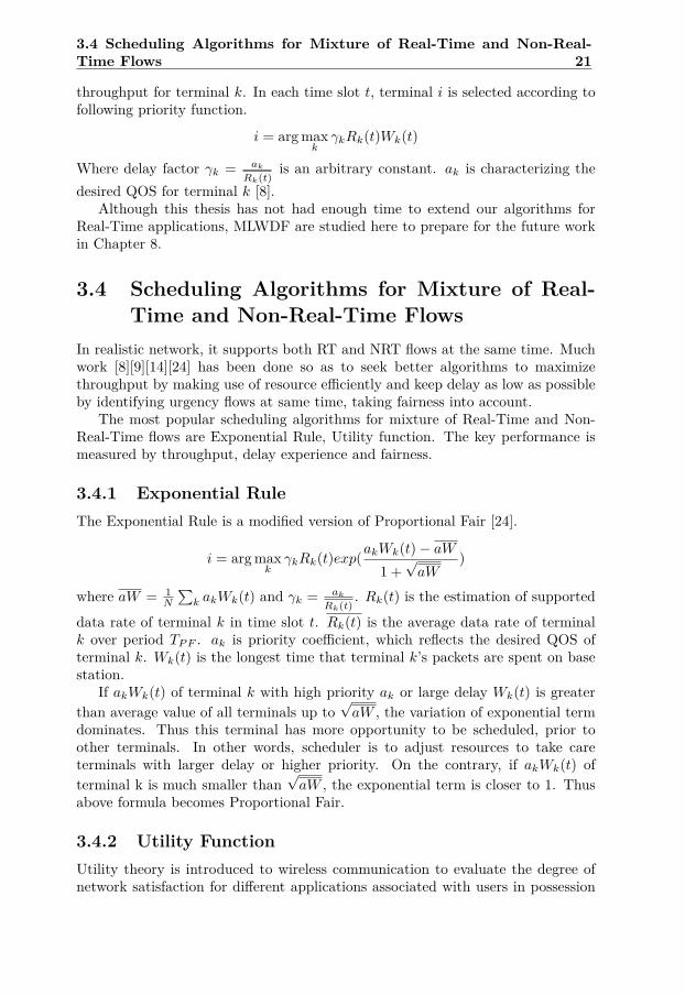
3.4 Scheduling Algorithms for Mixture of Real-Time and Non-Real-Time Flows
In realistic network, it supports both RT and NRT flows at the same time. Muchwork [8][9][14][24] has been done so as to seek better algorithms to maximizethroughput by making use of resource efficiently and keep delay as low as possibleby identifying urgency flows at same time, taking fairness into account.
The most popular scheduling algorithms for mixture of Real-Time and Non-Real-Time flows are Exponential Rule, Utility function. The key performance ismeasured by throughput, delay experience and fairness.
3.4.1 Exponential RuleThe Exponential Rule is a modified version of Proportional Fair [24].
i = arg maxk
γkRk(t)exp(akWk(t)− aW1 +√aW
)
where aW = 1N
∑k akWk(t) and γk = ak
Rk(t). Rk(t) is the estimation of supported
data rate of terminal k in time slot t. Rk(t) is the average data rate of terminalk over period TPF . ak is priority coefficient, which reflects the desired QOS ofterminal k. Wk(t) is the longest time that terminal k’s packets are spent on basestation.
If akWk(t) of terminal k with high priority ak or large delay Wk(t) is greaterthan average value of all terminals up to
√aW , the variation of exponential term
dominates. Thus this terminal has more opportunity to be scheduled, prior toother terminals. In other words, scheduler is to adjust resources to take careterminals with larger delay or higher priority. On the contrary, if akWk(t) ofterminal k is much smaller than
√aW , the exponential term is closer to 1. Thus
above formula becomes Proportional Fair.
3.4.2 Utility FunctionUtility theory is introduced to wireless communication to evaluate the degree ofnetwork satisfaction for different applications associated with users in possession
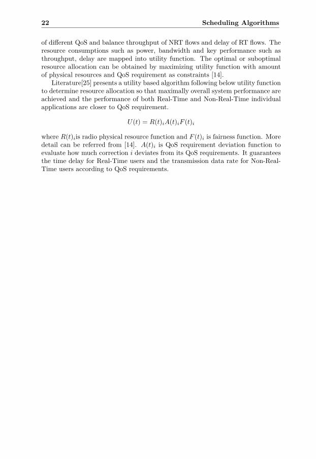
22 Scheduling Algorithms
of different QoS and balance throughput of NRT flows and delay of RT flows. Theresource consumptions such as power, bandwidth and key performance such asthroughput, delay are mapped into utility function. The optimal or suboptimalresource allocation can be obtained by maximizing utility function with amountof physical resources and QoS requirement as constraints [14].
Literature[25] presents a utility based algorithm following below utility functionto determine resource allocation so that maximally overall system performance areachieved and the performance of both Real-Time and Non-Real-Time individualapplications are closer to QoS requirement.
U(t) = R(t)iA(t)iF (t)i
where R(t)iis radio physical resource function and F (t)i is fairness function. Moredetail can be referred from [14]. A(t)i is QoS requirement deviation function toevaluate how much correction i deviates from its QoS requirements. It guaranteesthe time delay for Real-Time users and the transmission data rate for Non-Real-Time users according to QoS requirements.
Chapter 4
Scheduling Under a ControlSignaling Cost Constraint
4.1 BackgroundChapter 3 brings in several classic scheduling algorithms that make fully use oftime, frequency and space diversity to achieve the best performance. These al-gorithms are widely used in narrowband systems, but they cannot be applied towideband systems directly. One of the reasons is that these algorithms ignorethe signaling overhead caused by periodic scheduling map transmissions. In realapplications, terminals must exactly know which carrier conveys their data in cer-tain particular time slot for decoding. This information is packaged into schedul-ing map and transmitted to terminals via Physical Downlink Control Channel ofLTE. As discussed in Section 1.2, the control signaling overhead associated withthe scheduling maps can be significant, if the number of terminals or carriers islarge.
Much prior work has been done in order to mitigate the influence of signal-ing overhead on the overall system performance. It can be classified into threeapproaches. The first approach is to reduce the amount of control signaling bymerging contiguous resources into large blocks. As Section 2.3.2.2 said, 3GPPLong Term Evolution is implementing this technique to reduce the size of schedul-ing map [1], thus smaller signaling overhead is achieved. However, it causes thatsingle resource block cannot be scheduled even for small payload.
To avoid the influence of reduction of control signaling overhead on scheduling,the second approach is brought in. The reduction of control signaling overheadis carried out by making use of correlation and source coding. Reference [28]uses data compression technique to encode the control signaling. The compressionscheme composes of a run length coding, followed by a universal variable lengthcode. Reference [18] utilizes correlation of scheduling assignments for differentusers. The main idea is allowing a user with high SNR to overhear the schedulinginformation sent to other users with weaker SNR. Thus this user can deduce which
23

24 Scheduling Under a Control Signaling Cost Constraint
resource this user will not be scheduled based on the fact that no two users canshare the same resource at the same time. As a result, the cost of control signalingtransmitted to that user with high SNR can be avoided. The correlation betweenscheduling decision and CSI report is utilized in reference [21]. In the proposalof [21], mobiles make tentative scheduling decision and send to base station, andthen base station sends "agreement maps" to mobiles. As a result of correlationbetween tentative scheduling decision and agreement map, the signaling overheadcan be decreased with the help of source coding scheme.
For the last two approaches, the overall performance is increased after signaloverhead local optimization. To pursue global optimization, the third approachis exploited. In addition to encoding control signaling with compression scheme,signaling overhead as well as throughput is taken into account by scheduler. It ismodeled as nonlinear integer programming problem in reference [15]. Objectivefunction is maximizing net throughput instead of gross throughput. There are twoconstraints. The former one is the maximum number of subcarriers each terminalis allowed to have. The latter one is an objective fact that each subcarrier canbe assigned to a terminal at most. The optimal solution for above model resultsin huge computation. In order to simplify the computation, an approximationmodel is also proposed in [15], but the objective function value is not net through-put anymore. Even so, it is still hard to compute. Reference [12] formulates itas a combination problem, which is resolved by dynamic programming approachViterbi algorithm. The algorithm proposed by [12] is much flexible and closer topractical applications, compared with [15]. In [12], the number of subcarriers eachterminal can have is not fixed and the set of terminals selected for transmission aredepending on CSI and control signaling overhead. The most important advantageis that the optimal scheduling can be computed efficiently.
4.2 Proposed Scheduling Algorithm Under a Con-trol Signaling Cost Constraint for LTE/LTEAdvanced
4.2.1 NotationA subframe is a set of consecutively transmitted OFDM symbols, i.e. 7 × 2 = 14symbols. Referring to the introduction part of Chapter 3, the smallest resourceunit allowed to be assigned to one terminal is the schedule block, which is con-stituted by two successive PRBs. For convenience, this thesis still use resourceblock instead of schedule block as a unit for scheduling so that each resource blockconsists of 12 carriers for one subframe in duration. N is the amount of resourceblocks in one subframe.
K is the largest number of users that are allowed to be scheduled in a subframe.
U represents the set of users that will be scheduled in the subframe. u is thenumber of users in set U .
4.2 Proposed Scheduling Algorithm Under a Control Signaling CostConstraint for LTE/LTE Advanced 25
S stands for resource block assignment in one subframe based on U . Sn denotesthe index of user assigned to resource block n.
Cn(k) is the gross capacity of resource block n, if this resource block is assignedto terminal k.
ρ represents the set of control signaling coefficient ρi. ρi is control signaling coef-ficient for user i (i ∈ [1,K]). The value of ρi depends on service type. ρmax is themaximum value of control signaling coefficient of scheduled users set U .
A is control signaling cost penalty coefficient. The intention of introducing Ais to evaluate the influence of changing overall control signaling cost on through-put.
External water-filling represents the algorithm presented in Section 4.3.2, usedto find the optimal power assignment P for a given optimal resouce block assign-ment S.
Internal water-filling represents the algorithm introduced in Section 4.3.3, usedfor obtaining the optimal resource block assignment S and optimal power alloca-tion P for a given user set U .
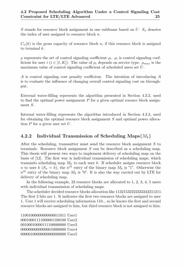
4.2.2 Individual Transmission of Scheduling Maps{Mk}After the scheduling, transmitter must send the resource block assignment S toterminals. Resource block assignment S can be described as a scheduling map.This thesis will present two ways to implement delivery of scheduling map on thebasis of [12]. The first way is individual transmission of scheduling maps, whichtransmits scheduling map Mk to each user k. If scheduler assigns resource blockn to user k (Sn = k), the nth entry of the binary map Mk is "1". Otherwise thenth entry of the binary map Mk is "0". It is also the way carried out by LTE fordelivery of scheduling map.
In the following example, 23 resource blocks are allocated to 1, 2, 3, 4, 5 userswith individual transmission of scheduling maps.
The scheduler decided resource blocks allocation like 11321532222333342211211.The first 2 bits are 1. It indicates the first two resource blocks are assigned to user1. User 1 will receive scheduling information 110.., so he knows the first and secondresource blocks are assigned to him, but third resource block is not assigned to him.
11001000000000000011011 User100010001111000001100100 User200100010000111100000000 User300000000000000010000000 User400000100000000000000000 User5
26 Scheduling Under a Control Signaling Cost Constraint
a) dlog2(N)e bits are assigned to each user and used for expressing the first intervallength. Since it is a constant value, add it to R. The initial value of n is equal to 0.
b) n=n+1.
c) Assign bits for the next interval length to each user, until n is equal to N .
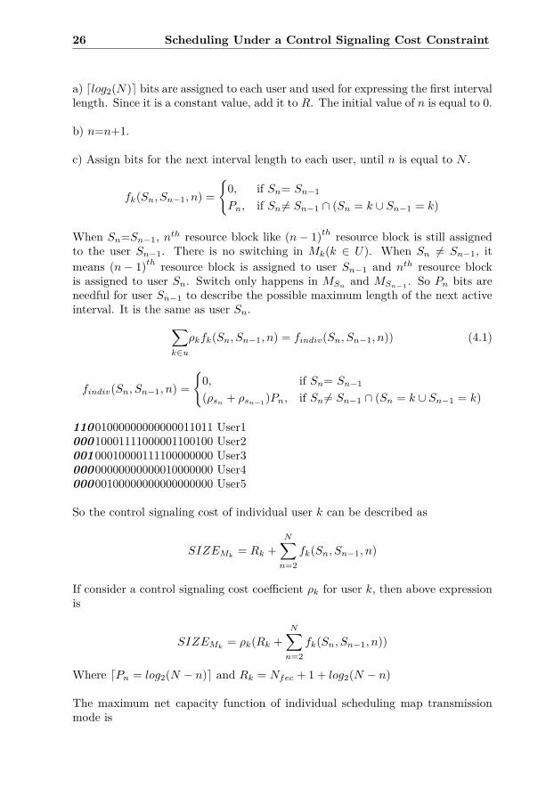
fk(Sn, Sn−1, n) ={
0, if Sn= Sn−1
Pn, if Sn 6= Sn−1 ∩ (Sn = k ∪ Sn−1 = k)
When Sn=Sn−1, nth resource block like (n− 1)th resource block is still assignedto the user Sn−1. There is no switching in Mk(k ∈ U). When Sn 6= Sn−1, itmeans (n− 1)th resource block is assigned to user Sn−1 and nth resource blockis assigned to user Sn. Switch only happens in MSn and MSn−1 . So Pn bits areneedful for user Sn−1 to describe the possible maximum length of the next activeinterval. It is the same as user Sn.∑
k∈u
ρkfk(Sn, Sn−1, n) = findiv(Sn, Sn−1, n)) (4.1)
findiv(Sn, Sn−1, n) ={
0, if Sn= Sn−1
(ρsn + ρsn−1)Pn, if Sn 6= Sn−1 ∩ (Sn = k ∪ Sn−1 = k)
11001000000000000011011 User100010001111000001100100 User200100010000111100000000 User300000000000000010000000 User400000100000000000000000 User5
So the control signaling cost of individual user k can be described as
SIZEMk= Rk +
N∑n=2
fk(Sn, Sn−1, n)
If consider a control signaling cost coefficient ρk for user k, then above expressionis
SIZEMk= ρk(Rk +
N∑n=2
fk(Sn, Sn−1, n))
Where dPn = log2(N − n)e and Rk = Nfec + 1 + log2(N − n)
The maximum net capacity function of individual scheduling map transmissionmode is

4.2 Proposed Scheduling Algorithm Under a Control Signaling CostConstraint for LTE/LTE Advanced 27
maxS
Cindiv(S) (4.2)
Where
Cindiv(S) =N∑n=1
Cn(Sn)−∑k∈u
ρk(Rk +N∑n=2
fk(Sn, Sn−1, n)) (4.3)
=N∑n=1
Cn(Sn)− (∑k∈u
ρkRk +∑k∈u
N∑n=2
ρkfk(Sn, Sn−1, n)) (4.4)
Since all Rk(k ∈ u) are equal, it can be replaced by R. The second term ofCindiv(S) is simplified with function (4.1).
Cindiv(S) =N∑n=1
Cn(Sn)− (R∑k∈u
ρk +∑k∈u
N∑n=2
ρkfk(Sn, Sn−1, n)) (4.5)
=N∑n=1
Cn(Sn)− (R∑k∈u
ρk +N∑n=2
findiv(Sn, Sn−1, n)) (4.6)
Insert a control signaling cost penalty A for all the users.
Cindiv(S) =N∑n=1
Cn(Sn)− (AR∑k∈u
ρk +A
N∑n=2
findiv(Sn, Sn−1, n)) (4.7)
4.2.3 Broadcasting of Joint Scheduling Map M
The entire resource block assignment S can also be represented with one jointscheduling map. This joint scheduling map is broadcasted to all the users.
Using the same example as 4.2.2, 23 resource blocks are allocated to 1, 2, 3, 4,5 users with broadcasting of joint scheduling map. The scheduler decided resourceblock allocation like 11321532222333342211211. After run length encoding, run-lengths of above example is [2, 1, 1, 1, 1, 1, 4, 4, 1, 2, 2, 1, 2] and indices of theusers that are assigned to the corresponding resource blocks is [1, 3, 2, 1, 5, 3, 2,3, 4, 2, 1, 2, 1].
a) Assign dlog2(N)e bits to each user for expressing the first interval length. Sinceit is a constant value, add it to R. The initial value of n is equal to 0.
R = |u|Lid +Nfec + dlog2(K)e+ dlog2(N)e
b) If n is not equal to N , increase n by 1. If yes, bits allocation is end.
28 Scheduling Under a Control Signaling Cost Constraint
c) If Sn = Sn−1 , go back b). Otherwise, implement d) and e).
d) Assign Pn bits to represent the possible maximum length of the next activeinterval when switching between two users in the map occurs.
dPn = log2(N − n)e
e) Assign Q bits to identify which user is being assigned to the resource blocks.
dQ = log2 |u|e
f) Repeat from b).The control signaling cost of all the users can be concluded as
SIZEM = R+N∑n=2
fbro(Sn, Sn−1, n)
where
fbro(Sn, Sn−1, n) ={
0, if Sn= Sn−1
Pn +Q, if Sn 6= Sn−1
Consider that the same network offers different service for different users, differ-ent service has different QoS requirement. It is more realistic to assign a specific ρkto a particular user k based on his service type. In broadcast mode, one schedul-ing map may include more than one user. The maximum ρ among users U inscheduling map is selected as a control signaling coefficient to measure how muchit costs to transmit one bit of control information in this map.The maximum net capacity function of broadcast scheduling map transmissionmode is
maxS
Cbro(S) (4.8)
Where
Cbro(S) =N∑n=1
Cn(Sn)− ρmax(R+N∑n=2
fbro(Sn, Sn−1, n)) (4.9)
Insert control signaling cost penalty A
Cbro(S) =N∑n=1
Cn(Sn)−Aρmax(R+N∑n=2
fbro(Sn, Sn−1, n)) (4.10)
4.2 Proposed Scheduling Algorithm Under a Control Signaling CostConstraint for LTE/LTE Advanced 29
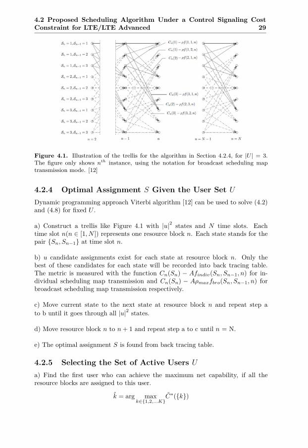
Figure 4.1. Illustration of the trellis for the algorithm in Section 4.2.4, for |U | = 3.The figure only shows nth instance, using the notation for broadcast scheduling maptransmission mode. [12]
4.2.4 Optimal Assignment S Given the User Set U
Dynamic programming approach Viterbi algorithm [12] can be used to solve (4.2)and (4.8) for fixed U .
a) Construct a trellis like Figure 4.1 with |u|2 states and N time slots. Eachtime slot n(n ∈ [1, N ]) represents one resource block n. Each state stands for thepair {Sn, Sn−1} at time slot n.
b) u candidate assignments exist for each state at resource block n. Only thebest of these candidates for each state will be recorded into back tracing table.The metric is measured with the function Cn(Sn) − Afindiv(Sn, Sn−1, n) for in-dividual scheduling map transmission and Cn(Sn) − Aρmaxfbro(Sn, Sn−1, n) forbroadcast scheduling map transmission respectively.
c) Move current state to the next state at resource block n and repeat step ato b until it goes through all |u|2 states.
d) Move resource block n to n+ 1 and repeat step a to c until n = N.
e) The optimal assignment S is found from back tracing table.
4.2.5 Selecting the Set of Active Users U
a) Find the first user who can achieve the maximum net capability, if all theresource blocks are assigned to this user.
k = arg maxk∈{1,2,...K}
C∗({k})

30 Scheduling Under a Control Signaling Cost Constraint
Set m = 1 and U (1) ={k}
b) Calculate possible overall capacity of u + 1 users, if one particular user inthe rest user list is added into U . Find the next user who would contribute themost to the overall capacity.
k = arg maxk∈{1,2,...K},k/∈U(m)
C∗(U (m) ∪ k)
c) Check if C∗(U (m) ∪ k) > C∗(U (m))If it is true, then user k will be added into U and m is increased by 1. Repeatfrom step b). Otherwise, return(U (m), S∗(U (m)), C∗(U (m))) [12].
4.3 Power OptimizationLet us assume an extreme situation. There is a resource block that causes ex-tremely low data rate for any user. According to the strategy of Section 4.2, thatresource block must be allocated to one user in U . Is it possible to ignore thatresource block? The answer is yes. We can save the power of certain resourceblocks, which yield low data rate due to some reason like distortion, and allocatethese power to other resource block which can bring higher data rate. Thus thetotal throughput can be increased, especially at low average power.
4.3.1 Water-fillingThe philosophy of water-filling algorithm is to allocate more power to sub-channelwith higher Signal to Noise Ratio (SNR) in order to maximize total throughputof all sub-channels, in the case of constant overall power.
Water-filling is the optimal algorithm for power allocation. It can be verifiedwith following mathematic derivative process. For OFDM transmission, a channelis divided into Nc independent sub-channels. Each sub-channel is corrupted byindependent white noise N0. Pn is the power allocated to nth sub-channel. hnis the channel impulse response between nth sub-channel and the terminal. Thebelow throughput expression of OFDM can be obtained with Shannon capacitybound formula.∑Nc−1n=0 log2(1 + Pn|hn|
N0
2) bits/OFDM symbol
Considering that the total power is fixed and hn is known from CSI, the maxi-mum throughput can be achieved by choosing proper Pn. This is a optimizationproblem. Objective function is (4.11), which subjects to (4.12).
CNc = maxp0...pNc−1
Nc−1∑n=0
log2(1 +Pn∣∣hn∣∣N0
2
) (4.11)
4.3 Power Optimization 31
Nc−1∑n=0
Pn = NcP, Pn ≥ 0, n = 0, ...Nc − 1 (4.12)
Since objective function is a jointly concave function. It can be solved withLagrangian method.
L(λ, P0, ..., PNc−1) =Nc−1∑n=0
log2(1 +Pn∣∣hn∣∣N0
2
)− λNc−1∑n=0
Pn (4.13)
Where λ is Lagrange multiplier.
P ∗n = ( 1λ− N0∣∣hn∣∣2 )
+(4.14)
P ∗n is the optimal power allocation of (4.11). If P ∗n < 0, P ∗n is assigned with 0,since power is impossible to be negative.
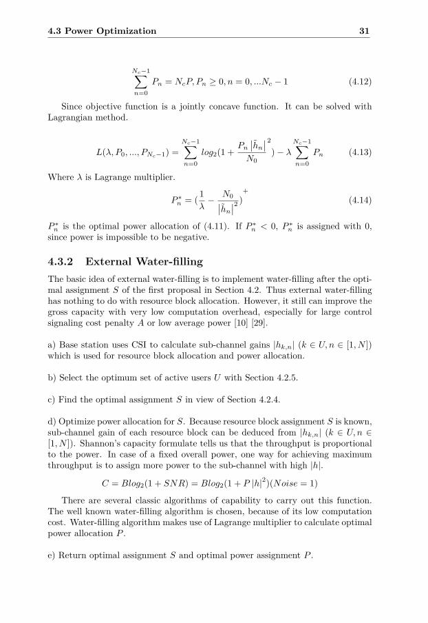
4.3.2 External Water-fillingThe basic idea of external water-filling is to implement water-filling after the opti-mal assignment S of the first proposal in Section 4.2. Thus external water-fillinghas nothing to do with resource block allocation. However, it still can improve thegross capacity with very low computation overhead, especially for large controlsignaling cost penalty A or low average power [10] [29].
a) Base station uses CSI to calculate sub-channel gains |hk,n| (k ∈ U, n ∈ [1, N ])which is used for resource block allocation and power allocation.
b) Select the optimum set of active users U with Section 4.2.5.
c) Find the optimal assignment S in view of Section 4.2.4.
d) Optimize power allocation for S. Because resource block assignment S is known,sub-channel gain of each resource block can be deduced from |hk,n| (k ∈ U, n ∈[1, N ]). Shannon’s capacity formulate tells us that the throughput is proportionalto the power. In case of a fixed overall power, one way for achieving maximumthroughput is to assign more power to the sub-channel with high |h|.
C = Blog2(1 + SNR) = Blog2(1 + P |h|2)(Noise = 1)
There are several classic algorithms of capability to carry out this function.The well known water-filling algorithm is chosen, because of its low computationcost. Water-filling algorithm makes use of Lagrange multiplier to calculate optimalpower allocation P .
e) Return optimal assignment S and optimal power assignment P .

32 Scheduling Under a Control Signaling Cost Constraint
4.3.3 Internal Water-fillingThe key factors of the scheduling in the first proposal are the data rate of eachuser achieved in a particular resource block and control signaling cost caused byassigning this particular resource block to a certain user. This is a two dimen-sions mathematic model. Internal water-filling is the upgraded version of the firstproposal. It extends mathematic model from two dimensions to three dimensions.Power control is the third dimension, besides channel condition and control sig-naling cost. Complexity mathematic model leads to huge computation cost. Evenso, it is still suboptimal solution due to mix integer programming problem.
a) Construct a trellis with |u|2 states and N time slots. Each time slot n′(n′ ∈[1, N ]) is corresponded to one resource block n′. Each state represents the pair{Sn, Sn−1} at time slot n′.
b) At the resource block n(n ∈ (1, N ]), each state has u candidate assignments.The best one is picked with the below metric functions and recorded into backtracing table.
Cindiv(S) =N∑n=1
Cn(Sn)− (AR∑k∈u
ρk +A∑k∈u
N∑n=2
ρkfk(Sn, Sn−1, n))
=N∑n=1
Cn(Sn)− (AR∑k∈u
ρk +A
N∑n=2
findiv(Sn, Sn−1, n))
=N∑n=1
Cn(Sn)−AR∑k∈u
ρk −AN∑n=2
findiv(Sn, Sn−1, n)
=N∑n=2
Cn(Sn)−AN∑n=2
findiv(Sn, Sn−1, n) + Cn(S1)−AR∑k∈u
ρk
Cbro(S) =N∑n=1
Cn(Sn)−Aρmax(R+N∑n=2
fbro(Sn, Sn−1, n))
=N∑n=1
Cn(Sn)−AρmaxR−AρmaxN∑n=2
fbro(Sn, Sn−1, n))
=N∑n=2
Cn(Sn)−AρmaxN∑n=2
fbro(Sn, Sn−1, n))−AρmaxR+ Cn(S1)
The metric associated with each branch is
n′∑n=2
(Cn(Sn)−Afindiv(Sn, Sn−1, n)) + Cn(S1)

4.4 Simulation Results 33
for individual scheduling map transmission mode and
n′∑n=2
(Cn(Sn)−Aρmaxfbro(Sn, Sn−1, n)) + Cn(S1)
for broadcast scheduling map transmission mode.
c) Find resource block assignment Si(i ∈ [1, n′]).Sn′ is the user occupying thecurrent resource block. Si(i ∈ [1, n′)). Sn′ is obtained with back tracing table.
d) Water-filling is implemented to optimize power allocation for Si(i ∈ [1, n′]).Sn′ .After power optimization, the gross capacity is obtained. The control signalingcost is calculated with f(Sn, Sn−1, n) and Si(i ∈ [1, n′]). Gross capacity minuscontrol signaling cost is net capacity. Fill net capacity into Viterbi table. If n isthe last resource block (n = N), power allocation scheme is recorded in the powertable.
e) Move current state to the next state at resource block n′ and repeat step a) tod) until current state is equal to |u|2.
f) Move resource block n′ to n′ + 1 and repeat step a) to e) until n = N .
g) Deduct extra bits for map initialization from net capacity. Extra bits areAR
∑k∈u
ρk for individual scheduling map transmission mode and AρmaxR for broad-
cast scheduling map transmission mode.
4.4 Simulation Results
4.4.1 Individual and Broadcast Scheduling Map Transmis-sion
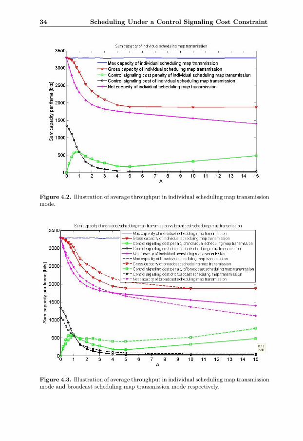
The algorithms of individual scheduling map transmission and broadcast schedul-ing map transmission are designed for LTE OFDMA system. Figure 4.2 illus-trates the operation of resource block assignment for a LTE OFDMA system with18 MHz bandwidth using the proposed algorithm of individual scheduling maptransmission. The bandwidth per resource block is 180kHz and each frame hasten OFDM symbols. The independent and identically distributed (i.i.d.) Rayleighfading channel is chosen for this simulation. When A is near zero, scheduler selectsthe users with slightly better channel conditions due to negligible control signalingcost. It leads to high gross capacity and high control signaling cost at the sametime, as shown in Figure 4.2. As A increasing, control signaling cost becomesthe primary factor for scheduler. It indicates that the scheduler prefers to assignresource block to the owner of the last resource block in order to avoid the costof control signaling. That is why the control signaling cost is decreasing instead
34 Scheduling Under a Control Signaling Cost Constraint
Figure 4.2. Illustration of average throughput in individual scheduling map transmissionmode.
Figure 4.3. Illustration of average throughput in individual scheduling map transmissionmode and broadcast scheduling map transmission mode respectively.
4.4 Simulation Results 35
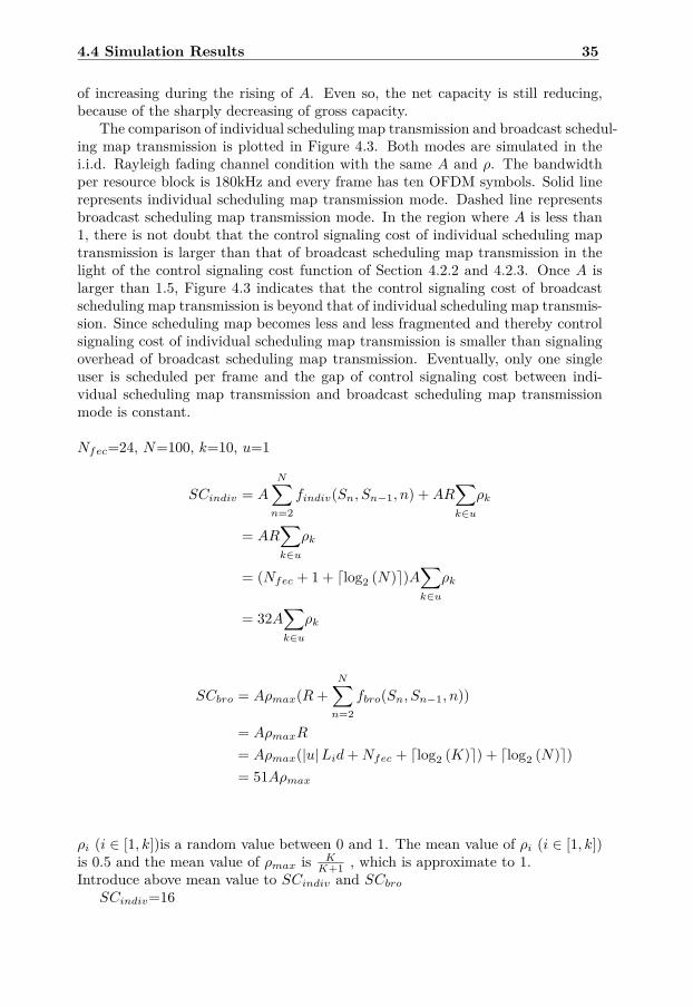
of increasing during the rising of A. Even so, the net capacity is still reducing,because of the sharply decreasing of gross capacity.
The comparison of individual scheduling map transmission and broadcast schedul-ing map transmission is plotted in Figure 4.3. Both modes are simulated in thei.i.d. Rayleigh fading channel condition with the same A and ρ. The bandwidthper resource block is 180kHz and every frame has ten OFDM symbols. Solid linerepresents individual scheduling map transmission mode. Dashed line representsbroadcast scheduling map transmission mode. In the region where A is less than1, there is not doubt that the control signaling cost of individual scheduling maptransmission is larger than that of broadcast scheduling map transmission in thelight of the control signaling cost function of Section 4.2.2 and 4.2.3. Once A islarger than 1.5, Figure 4.3 indicates that the control signaling cost of broadcastscheduling map transmission is beyond that of individual scheduling map transmis-sion. Since scheduling map becomes less and less fragmented and thereby controlsignaling cost of individual scheduling map transmission is smaller than signalingoverhead of broadcast scheduling map transmission. Eventually, only one singleuser is scheduled per frame and the gap of control signaling cost between indi-vidual scheduling map transmission and broadcast scheduling map transmissionmode is constant.
Nfec=24, N=100, k=10, u=1
SCindiv = A
N∑n=2
findiv(Sn, Sn−1, n) +AR∑k∈u
ρk
= AR∑k∈u
ρk
= (Nfec + 1 + dlog2 (N)e)A∑k∈u
ρk
= 32A∑k∈u
ρk
SCbro = Aρmax(R+N∑n=2
fbro(Sn, Sn−1, n))
= AρmaxR
= Aρmax(|u|Lid+Nfec + dlog2 (K)e) + dlog2 (N)e)= 51Aρmax
ρi (i ∈ [1, k])is a random value between 0 and 1. The mean value of ρi (i ∈ [1, k])is 0.5 and the mean value of ρmax is K
K+1 , which is approximate to 1.Introduce above mean value to SCindiv and SCbro
SCindiv=16

36 Scheduling Under a Control Signaling Cost Constraint
Figure 4.4. Illustration of average throughput in individual scheduling map transmis-sion mode and broadcast scheduling map transmission mode based on individual subcar-riers. Solid line represents individual scheduling map transmission mode. Dashed linerepresents broadcast scheduling map transmission mode.
SCbro=51When only one signal user is scheduled per frame, the control signaling cost of in-dividual scheduling map transmission and broadcast scheduling map transmissionare 16 and 51 respectively. These derivations can be proven by Figure 4.3
The similar configuration as Figure 4.3 is implemented in Figure 4.4. The onlydifference is that scheduling is based on individual subcarriers, instead of resourceblock, which consists of 12 subcarriers. It is natural that the control signaling costis much larger. Comparing with 4.3, the net capacity of both modes fall downsharply, when A is small. That is because of large control signaling overhead.
The simulation environment of Figure 4.5 likes Figure 4.3, except the param-eters of Rayleigh fading channel. The 3GPP Extended Vehicular A power delayprofile is set for the Rayleigh fading channels of the simulation. Figure 4.5 pointsout that its gross capacity and net capacity outperform those of Figure 4.3. It prof-its from the correlation between channel and frequency. The correlation makes theusers have an opportunity to have high channel gains at numerous frequencies.
4.4.2 External Water-fillingThe reason why we present plots of gross capacity instead of net capacity is thatexternal water-filling does not bring any additional control signaling cost so thatincreased gross capacity can be consider as increased net capacity. From Figure

4.4 Simulation Results 37
Figure 4.5. Illustration of average throughput of individual scheduling map transmissionmode and broadcast scheduling map mode in the Rayleigh fading channel following the3GPP Extended Vehicular A power delay profile.
Figure 4.6. Illustration of increased gross capacity ratio of external water-filling inindividual scheduling map transmission mode, referring to gross capacity of equal powerassignment. The bandwidth per resource block is 180kHz and every frame has ten OFDMsymbols. The channel condition is Rayleigh fading channel.

38 Scheduling Under a Control Signaling Cost Constraint
4.6, we can see that the gross capacity of individual scheduling map transmission isimproved apparently by using external water-filling algorithm. The plots of Figure4.6 is obtained by the below function.
GIncreased [%] = G2−G1G1
where G1 is the gross capacity of the first proposal without power optimization,G2 is the gross capacity of external water-filling.
It is obvious that as the average power is increasing, the increased gross capacityis decreasing. Finally, the increased gross capacity is close to 0 due to the fact thatthe individual power is increasing corresponding to the rising of the overall averagepower. Thus power optimization has less and less impact on gross capacity. Onthe contrary, the external water-filling generates large gain for the case of lowaverage power.
Furthermore, increased gross capacity relies on the control signaling cost, sincecontrol signaling cost affects scheduling. The control signaling cost is relating tocontrol signaling cost coefficient ρ and control signaling cost penalty coefficient A.With the growing of ρ and A, the control signaling cost due to switching betweenusers may be larger than increased data rate caused by switching users. In thissituation, scheduler prefers to select the same user as the last resource block ratherthan switching to another user with the higher data rate. It changes resourceblock assignment S, which results in variation in sub-channel gain distributionof S. The intention of external water-filling is to make use of this variation toachieve higher gross capacity. When the most sub-channels of S are located inlower gain in distribution, external water-filling can have excellent performance.The sub-channel gain distribution will be discussed in the Figure 4.7.
Figure 4.6 concludes that external water-filling can contribute more extra gainby optimizing power distribution. It can be explained with Figure 4.7. For A=0,control signaling cost is for free. Scheduler chooses the user who can achievemaximum data rate in that resource block. Data rate is determined by C =Blog2(1 + SNR) = Blog2(1 + P |h|2) where B, P is fixed for each user, so the userwith the higher sub-channel gain |h|2 in that resource block will be chosen. It isverified by Figure 4.7. When A=0, the most sub-channel gains of S are distributedin the high level. It leads to a very slight improvement of gross capacity for A=0in Figure 4.6.
For A =12, control signaling penalty is significant. Scheduler selects users toobtain maximum net capacity, which is gross capacity minus control signaling cost.The most sub-channel gains of S are distributed in the low level in order to avoidswitching in view of control signaling cost. Hence, there is a large space to improvegross capacity by optimizing power allocation. However, Figure 4.6 shows that itis merely a slight raise for increased data rate with the increasing of A from 3to 12. It can be explained easily with Figure 4.7. Sub-channel gain distributionis almost not changing, when A reaches the threshold value that the first factorconsidered by scheduler is switched from data rate of individual resource block tocontrol signaling cost.
The increased gross capacity of external water-filling and sub-channel gain

4.4 Simulation Results 39
Figure 4.7. Illustration of sub-channel gain distribution of optimal assignment S inindividual scheduling map transmission mode. Figure 4.7 is simulated in the same con-figuration as Figure 4.6, but sub-channel gains are measured before optimizing power.
Figure 4.8. Illustration of increased gross capacity of external water-filling in broadcastscheduling map transmission mode.
40 Scheduling Under a Control Signaling Cost Constraint
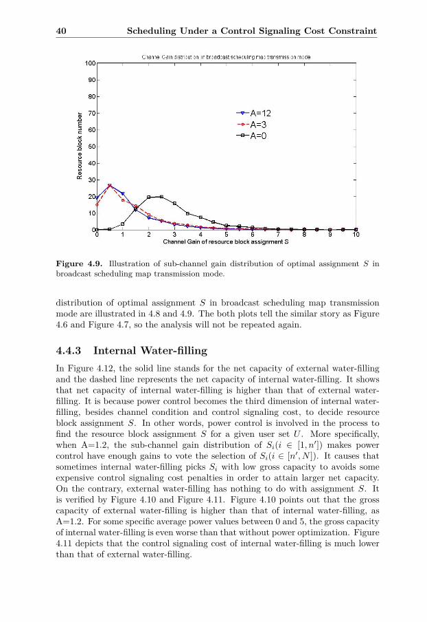
Figure 4.9. Illustration of sub-channel gain distribution of optimal assignment S inbroadcast scheduling map transmission mode.
distribution of optimal assignment S in broadcast scheduling map transmissionmode are illustrated in 4.8 and 4.9. The both plots tell the similar story as Figure4.6 and Figure 4.7, so the analysis will not be repeated again.
4.4.3 Internal Water-fillingIn Figure 4.12, the solid line stands for the net capacity of external water-fillingand the dashed line represents the net capacity of internal water-filling. It showsthat net capacity of internal water-filling is higher than that of external water-filling. It is because power control becomes the third dimension of internal water-filling, besides channel condition and control signaling cost, to decide resourceblock assignment S. In other words, power control is involved in the process tofind the resource block assignment S for a given user set U . More specifically,when A=1.2, the sub-channel gain distribution of Si(i ∈ [1, n′]) makes powercontrol have enough gains to vote the selection of Si(i ∈ [n′, N ]). It causes thatsometimes internal water-filling picks Si with low gross capacity to avoids someexpensive control signaling cost penalties in order to attain larger net capacity.On the contrary, external water-filling has nothing to do with assignment S. Itis verified by Figure 4.10 and Figure 4.11. Figure 4.10 points out that the grosscapacity of external water-filling is higher than that of internal water-filling, asA=1.2. For some specific average power values between 0 and 5, the gross capacityof internal water-filling is even worse than that without power optimization. Figure4.11 depicts that the control signaling cost of internal water-filling is much lowerthan that of external water-filling.
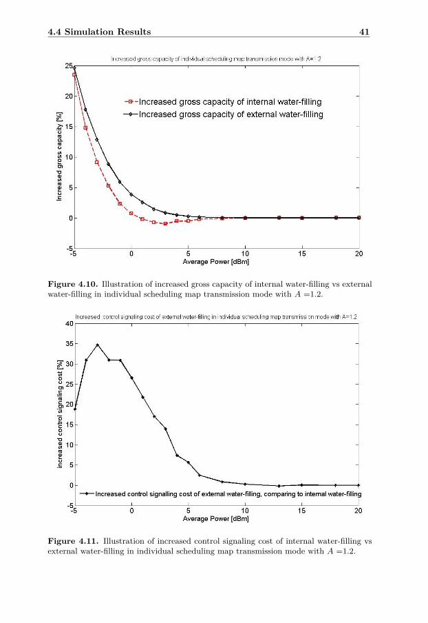
4.4 Simulation Results 41
Figure 4.10. Illustration of increased gross capacity of internal water-filling vs externalwater-filling in individual scheduling map transmission mode with A =1.2.
Figure 4.11. Illustration of increased control signaling cost of internal water-filling vsexternal water-filling in individual scheduling map transmission mode with A =1.2.
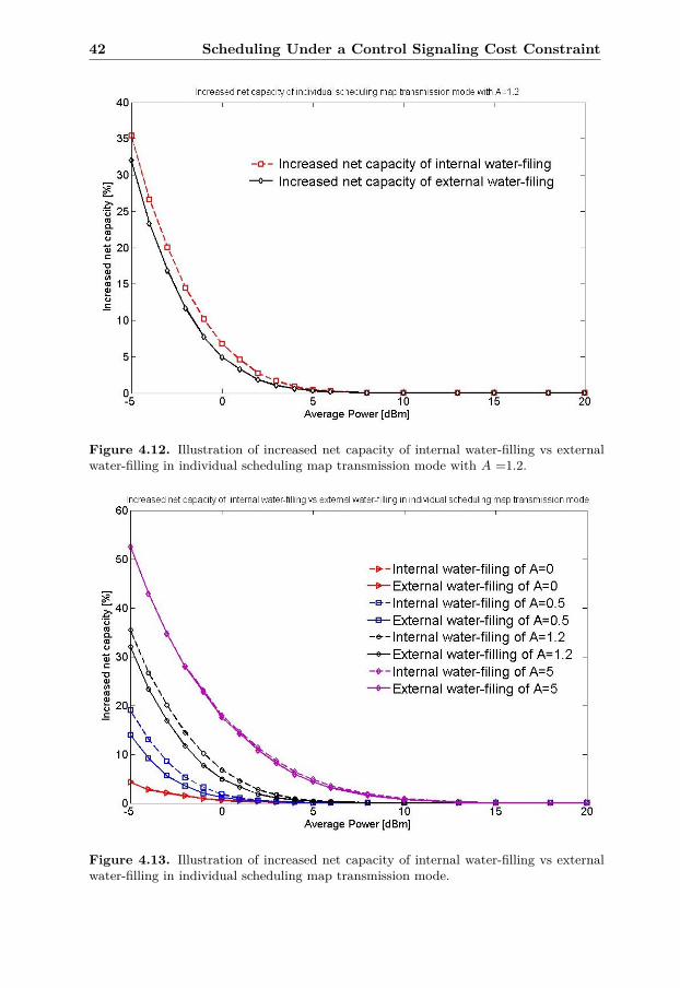
42 Scheduling Under a Control Signaling Cost Constraint
Figure 4.12. Illustration of increased net capacity of internal water-filling vs externalwater-filling in individual scheduling map transmission mode with A =1.2.
Figure 4.13. Illustration of increased net capacity of internal water-filling vs externalwater-filling in individual scheduling map transmission mode.
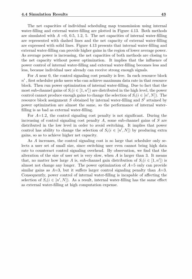
4.4 Simulation Results 43
The net capacities of individual scheduling map transmission using internalwater-filling and external water-filling are plotted in Figure 4.13. Both methodsare simulated with A =0, 0.5, 1.2, 5. The net capacities of internal water-fillingare represented with dashed lines and the net capacity of external water-fillingare expressed with solid lines. Figure 4.13 presents that internal water-filling andexternal water-filling can provide higher gains in the region of lower average power.As average power is increasing, the net capacities of both methods are closing tothe net capacity without power optimization. It implies that the influence ofpower control of internal water-filling and external water-filling becomes less andless, because individual user already can receive strong enough signals.
For A near 0, the control signaling cost penalty is free. In each resource blockn′ , first scheduler picks users who can achieve maximum data rate in that resourceblock. Then run power optimization of internal water-filling. Due to fact that themost sub-channel gains of Si(i ∈ [1, n′]) are distributed in the high level, the powercontrol cannot produce enough gains to change the selection of Si(i ∈ [n′, N ]). Theresource block assignment S obtained by internal water-filling and S′ attained bypower optimization are almost the same, so the performance of internal water-filling is as bad as external water-filling.
For A=1.2, the control signaling cost penalty is not significant. During theincreasing of control signaling cost penalty A, some sub-channel gains of S aredistributed in the low level in order to avoid switching. It implies that powercontrol has ability to change the selection of Si(i ∈ [n′, N ]) by producing extragains, so as to achieve higher net capacity.
As A increases, the control signaling cost is so large that scheduler only se-lects a user set of small size, since switching user even cannot bring high datarate to counteract control signaling overhead. By observation, we find that thealteration of the size of user set is very slow, when A is larger than 3. It meansthat, no matter how large A is, sub-channel gain distribution of Si(i ∈ [1, n′]) isalmost not change any longer. The power optimization of A=5 only can providesimilar gains as A=3, but it suffers larger control signaling penalty than A=3.Consequently, power control of internal water-filling is incapable of affecting theselection of Si(i ∈ [n′, N ]). As a result, internal water-filling has the same effectas external water-filling at high computation expense.
44 Scheduling Under a Control Signaling Cost Constraint

Chapter 5
Adaptive Length Subframe
5.1 Rayleigh Fading ChannelRayleigh fading channel model is a suitable model for urban area where thereis no line of sight propagation between transmitters and receivers. Transmittedsignals suffer attenuation, reflection, refraction and diffraction, before reaching thereceivers. If the number of reflections is large, the channel impulse response can beconsidered as Gaussian process according to the central limit theorem. Since thereis no direct signal component in Rayleigh fading channel model, the process haszero mean and evenly distributed phase between 0 and 2π. Therefore, the envelopeof channel response is distributed corresponding to Rayleigh distribution.
There are many approaches to model and simulate Rayleigh fading channel.In this thesis, an improved sum-of-sinusoids simulation model [30] is used to sim-ulate Rayleigh fading channel. The improved sum-of-sinusoids simulation modelproposes a new way to simplify the Clark’s reference model.
The reference nonselective fading of Clark’s reference model is expressed by
g(t) =√
2N
N∑n=1
e[j(wdtcosαn+φn)] (5.1)
where αn is the angle of incoming wave, φn is the initial phase for nth propagationpath, and wd is the maximum angular Doppler frequency.
(5.1) can be transformed to (5.2) by reasonable assumptions and algebraicmanipulation [30].
g(t) =√
2N
{M∑n=1
2cos(wdtcosαn + φn) + j
M∑n=1
2cos(wdtsinαn + φn)}
(5.2)
Except N = 4M , other parameters of (5.2) have the same meaning as those of(5.1). For simplification, the real part and imaginary part of (5.2) are expressedwith Zc and Zs in (5.3)respectively.
45
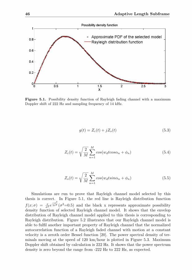
46 Adaptive Length Subframe
Figure 5.1. Possibility density function of Rayleigh fading channel with a maximumDoppler shift of 222 Hz and sampling frequency of 14 kHz.
g(t) = Zc(t) + jZs(t) (5.3)
Zc(t) =√
2M
M∑n=1
cos(wdtcosαn + φn) (5.4)
Zs(t) =√
2M
M∑n=1
cos(wdtsinαn + φn) (5.5)
Simulations are run to prove that Rayleigh channel model selected by thisthesis is correct. In Figure 5.1, the red line is Rayleigh distribution functionf(x;σ) = x
σ2 e−x2
2σ2 (σ2=0.5) and the black x represents approximate possibilitydensity function of selected Rayleigh channel model. It shows that the envelopdistribution of Rayleigh channel model applied to this thesis is corresponding toRayleigh distribution. Figure 5.2 illustrates that our Rayleigh channel model isable to fulfil another important property of Rayleigh channel that the normalizedautocorrelation function of a Rayleigh faded channel with motion at a constantvelocity is a zeroth order Bessel function [20]. The power spectral density of ter-minals moving at the speed of 120 km/hour is plotted in Figure 5.3. MaximumDoppler shift obtained by calculation is 222 Hz. It shows that the power spectrumdensity is zero beyond the range from -222 Hz to 222 Hz, as expected.
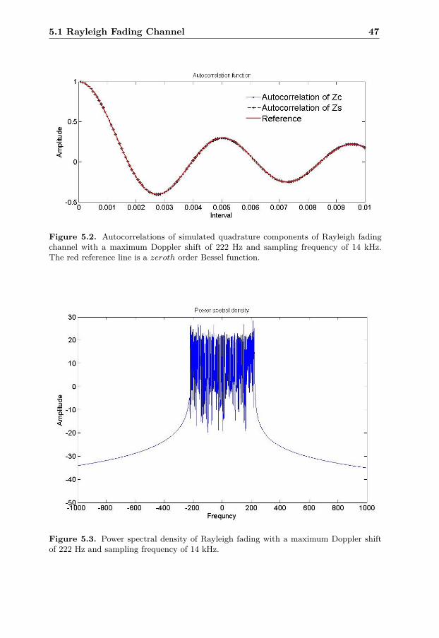
5.1 Rayleigh Fading Channel 47
Figure 5.2. Autocorrelations of simulated quadrature components of Rayleigh fadingchannel with a maximum Doppler shift of 222 Hz and sampling frequency of 14 kHz.The red reference line is a zeroth order Bessel function.
Figure 5.3. Power spectral density of Rayleigh fading with a maximum Doppler shiftof 222 Hz and sampling frequency of 14 kHz.
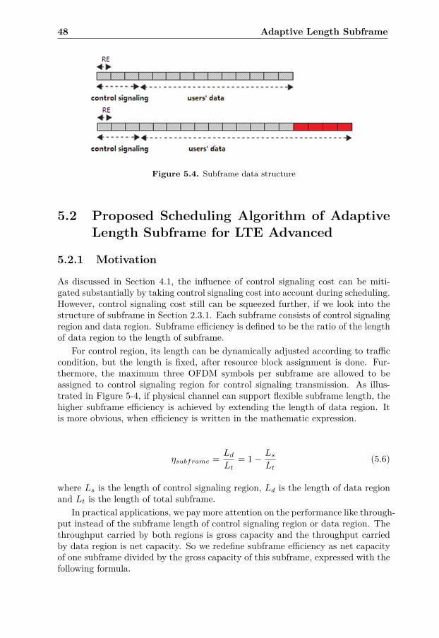
48 Adaptive Length Subframe
Figure 5.4. Subframe data structure
5.2 Proposed Scheduling Algorithm of AdaptiveLength Subframe for LTE Advanced
5.2.1 Motivation
As discussed in Section 4.1, the influence of control signaling cost can be miti-gated substantially by taking control signaling cost into account during scheduling.However, control signaling cost still can be squeezed further, if we look into thestructure of subframe in Section 2.3.1. Each subframe consists of control signalingregion and data region. Subframe efficiency is defined to be the ratio of the lengthof data region to the length of subframe.
For control region, its length can be dynamically adjusted according to trafficcondition, but the length is fixed, after resource block assignment is done. Fur-thermore, the maximum three OFDM symbols per subframe are allowed to beassigned to control signaling region for control signaling transmission. As illus-trated in Figure 5-4, if physical channel can support flexible subframe length, thehigher subframe efficiency is achieved by extending the length of data region. Itis more obvious, when efficiency is written in the mathematic expression.
ηsubframe = LdLt
= 1− LsLt
(5.6)
where Ls is the length of control signaling region, Ld is the length of data regionand Lt is the length of total subframe.
In practical applications, we pay more attention on the performance like through-put instead of the subframe length of control signaling region or data region. Thethroughput carried by both regions is gross capacity and the throughput carriedby data region is net capacity. So we redefine subframe efficiency as net capacityof one subframe divided by the gross capacity of this subframe, expressed with thefollowing formula.

5.2 Proposed Scheduling Algorithm of Adaptive Length Subframe forLTE Advanced 49
ηsubframe = Cg(l)− CsCg(l)
= 1− CsCg(l)
(5.7)
where l is the length of subframe, Cg(l) and Cn(l) denotes the gross capacity andnet capacity of this subframe respectively, and Cs(l) is the control signaling cost.
With the increasing of subframe length, the subframe efficiency is infinitelyapproaching to 1. On one hand, the overall control signaling cost is further re-ducing with the help of extending subframe length. On the other hand, overlongsubframe can result in large latency and low average data rate (bits/symbol). Anew algorithm to pursue optimal tradeoff between subframe efficiency and averagedata rate is proposed in this chapter.
5.2.2 Subframe Length Optimization AlgorithmThe purpose of this algorithm is to find the optimal subframe length so that thesystem can achieve as high subframe efficiency as possible, while keeping the max-imum average data rate. The subframe length optimization algorithm can bedescribed as the following steps.
a) Assume the channels between base station and terminals are Rayleigh fadingchannels, following the 3GPP Extended Vehicular A power delay profile. Thereare K users in the target base station. Each subframe has N resource blocks likeSection 4.2.1. i is the index of OFDM symbol, of which initial value is 1. Csumis the system gross capacity and is initialled by 0. Cave is the system average netcapacity (bits/symbol). Its initial value is 0.
b) Terminals feedback channel conditions with CSI, after receiving reference sig-nal. The base station uses CSI to estimate channel gain function |hk,n| (t)(k ∈[1,K] , n ∈ [1, N ]) which will be used to determine scheduling and subframe length.
c) Gross capacity matrix of all the users and resource blocks within the i symbolcan be counted like this.Ck,n(i− 1) = Blog2(1 + P |hk,n|2)(Noise = 1, k ∈ [1,K] , n ∈ [1, N ] , i ∈ [1, 140])If i is equal to 1, execute d) and e). Otherwise, jump to f) directly.
d) Select the optimal set U of active users based on Ck,n(0), referring to Sec-tion 4.2.4.
e) Find the optimal assignment S with Ck,n(0), using the method in the Sec-tion 4.2.5.
f) Csum=Csum+Cs(i)where Cs(i) is the gross capacity within symbol i and obtained with the help ofoptimal assignment S and Ck,n(i− 1).If i is equal to 1, Csum=Csum - Ccs.

50 Adaptive Length Subframe
Figure 5.5. Average data rate of broadcast scheduling map and individual schedulingmap transmission modes as function of subframe length, with control signaling costpenalty coefficient A=1. The channel is Rayleigh fading channel, following the 3GPPExtended Vehicular A power delay profile.
where Ccs is control signaling cost and computed with the optimal assignment S.
g) System average net capacity can be calculated by Cave(i) = Csumi
If Cave(i)>=Cave(i − 1) , then i will be increased by 1 and repeat from c). Oth-erwise, return {U, S, i− 1}
5.3 Simulation Results
5.3.1 Optimal Subframe Length for Individual and Broad-cast Scheduling Map Transmission Modes
Figure 5.5 shows that the Cave(bits per symbol) of broadcast scheduling maptransmission and individual scheduling map transmission reach maximum, whensubframe length is 9 and 10 respectively in the case of control signaling cost penaltyA=1. The reasons why average data rate of broadcast scheduling map transmissionis beyond average data rate of individual scheduling map transmission are thatthe gross capacity of broadcast scheduling map transmission is higher than thatof individual scheduling map mode and the control signaling cost of broadcastscheduling map mode is lower than that of individual scheduling map transmissionin the case of control signaling cost penalty A=1, as illustrated in Figure 5.6. In
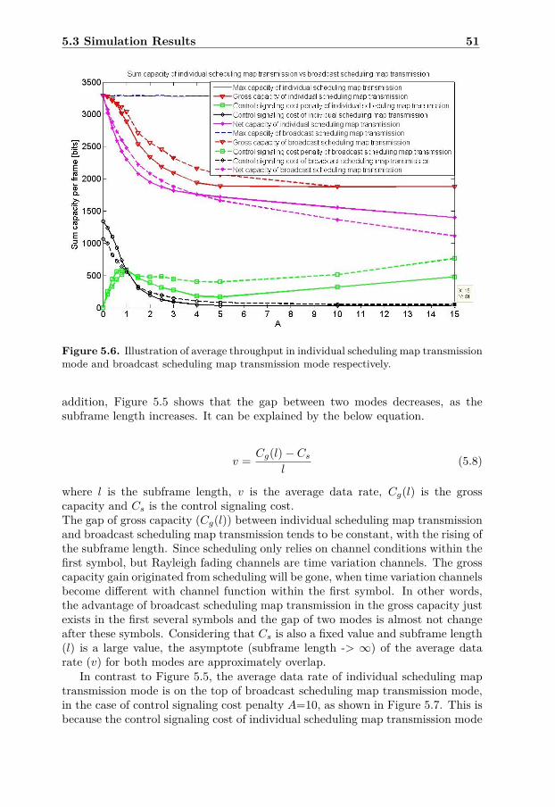
5.3 Simulation Results 51
Figure 5.6. Illustration of average throughput in individual scheduling map transmissionmode and broadcast scheduling map transmission mode respectively.
addition, Figure 5.5 shows that the gap between two modes decreases, as thesubframe length increases. It can be explained by the below equation.
v = Cg(l)− Csl
(5.8)
where l is the subframe length, v is the average data rate, Cg(l) is the grosscapacity and Cs is the control signaling cost.The gap of gross capacity (Cg(l)) between individual scheduling map transmissionand broadcast scheduling map transmission tends to be constant, with the rising ofthe subframe length. Since scheduling only relies on channel conditions within thefirst symbol, but Rayleigh fading channels are time variation channels. The grosscapacity gain originated from scheduling will be gone, when time variation channelsbecome different with channel function within the first symbol. In other words,the advantage of broadcast scheduling map transmission in the gross capacity justexists in the first several symbols and the gap of two modes is almost not changeafter these symbols. Considering that Cs is also a fixed value and subframe length(l) is a large value, the asymptote (subframe length -> ∞) of the average datarate (v) for both modes are approximately overlap.
In contrast to Figure 5.5, the average data rate of individual scheduling maptransmission mode is on the top of broadcast scheduling map transmission mode,in the case of control signaling cost penalty A=10, as shown in Figure 5.7. This isbecause the control signaling cost of individual scheduling map transmission mode
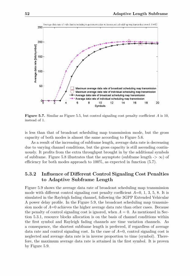
52 Adaptive Length Subframe
Figure 5.7. Similar as Figure 5.5, but control signaling cost penalty coefficient A is 10,instead of 1.
is less than that of broadcast scheduling map transmission mode, but the grosscapacity of both modes is almost the same according to Figure 5.6.
As a result of the increasing of subframe length, average data rate is decreasingdue to varying channel conditions, but the gross capacity is still ascending contin-uously. It profits from the extra throughput brought in by the additional symbolsof subframe. Figure 5.8 illustrates that the asymptote (subframe length -> ∞) ofefficiency for both modes approach to 100%, as expected in function (5.7).
5.3.2 Influence of Different Control Signaling Cost Penaltiesto Adaptive Subframe Length
Figure 5.9 shows the average data rate of broadcast scheduling map transmissionmode with different control signaling cost penalty coefficient A=0, 1, 3, 5, 8. It issimulated in the Rayleigh fading channel, following the 3GPP Extended VehicularA power delay profile. In the Figure 5.9, the broadcast scheduling map transmis-sion mode of A=0 achieves the higher average data rate than other cases. Becausethe penalty of control signaling cost is ignored, when A = 0. As mentioned in Sec-tion 5.3.1, resource blocks allocation is on the basis of channel conditions withinthe first symbol and Rayleigh fading channels are time variation channels. Asa consequence, the shortest subframe length is preferred, if regardless of averagedata rate and control signaling cost. In the case of A=0, control signaling cost isneglected and average data rate is in inverse proportion to time (symbol). There-fore, the maximum average data rate is attained in the first symbol. It is provenby Figure 5.9.
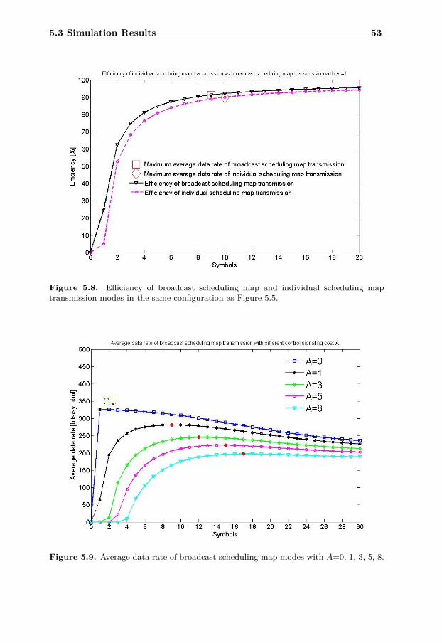
5.3 Simulation Results 53
Figure 5.8. Efficiency of broadcast scheduling map and individual scheduling maptransmission modes in the same configuration as Figure 5.5.
Figure 5.9. Average data rate of broadcast scheduling map modes with A=0, 1, 3, 5, 8.
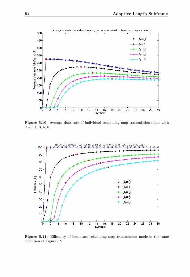
54 Adaptive Length Subframe
Figure 5.10. Average data rate of individual scheduling map transmission mode withA=0, 1, 3, 5, 8.
Figure 5.11. Efficiency of broadcast scheduling map transmission mode in the samecondition of Figure 5.9.

5.3 Simulation Results 55
Figure 5.12. Efficiency of individual scheduling map transmission mode in the samecondition of Figure 5.10.
The average data rate of individual scheduling map transmission mode withcontrol signaling cost penalty coefficient A=0, 1, 3, 5, 8 is plotted in Figure 5.10.Similar to broadcast scheduling map transmission mode, the higher average datarate is in the case of A=0 and the first symbol of A=0 reaches the maximumaverage data rate.
Figure 5.11 and Figure 5.12 illustrate the efficiency of broadcast and individualscheduling map transmission modes in the case of control signaling cost penaltyA=0, 1, 3, 5, 8, via the Rayleigh fading channels. It is apparent that the asymptote(subframe length ->∞) of efficiency for both modes approach to 100%. The reasonis discussed in the Section 5.3.1.
5.3.3 Influence of Doppler Frequency to Adaptive SubframeLength
Figure 5.13 shows that the average data rate of terminals are moving with the speedof V=1, 5, 25, 120, 300 km/h. The channel is Rayleigh fading channel, followingthe 3GPP Extended Vehicular A power delay profile. For terminals whose averagespeed is less than 1 km/h, they can be considered stillness under the base station.The rest moving speeds of terminals in simulation (V=5, 25, 120, 300 km/h) referto average human walking speed, bicycle, vehicle, high speed train. We can seethat the higher speed terminals move, the shorter optimal subframe length it is.In other words, the optimal subframe length is inversely proportion to the speed.
The aforementioned phenomenon is caused by the variation of channel condi-tions. The higher speed terminals are moving, the severer fading the channel willbe. When terminals are still, the channels between terminals and base station can
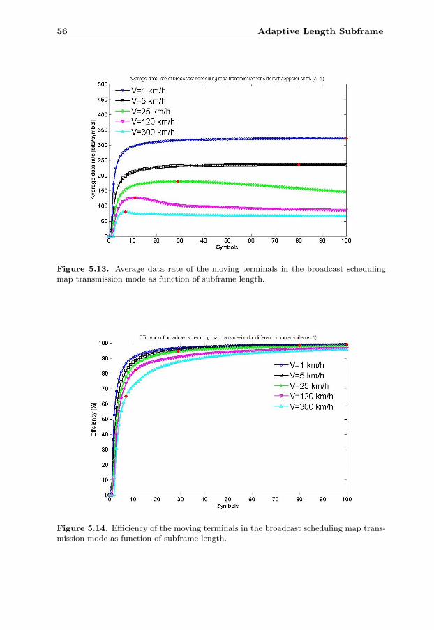
56 Adaptive Length Subframe
Figure 5.13. Average data rate of the moving terminals in the broadcast schedulingmap transmission mode as function of subframe length.
Figure 5.14. Efficiency of the moving terminals in the broadcast scheduling map trans-mission mode as function of subframe length.
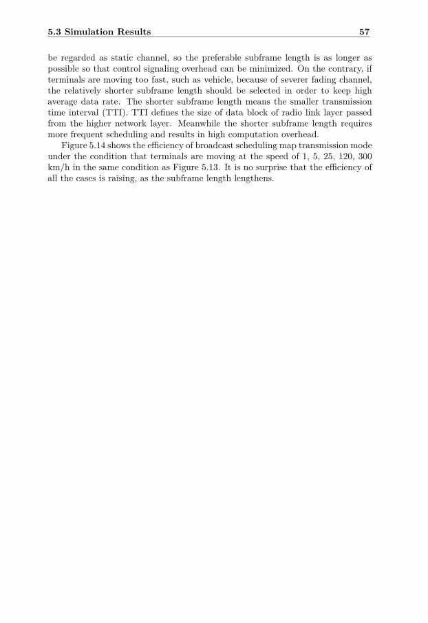
5.3 Simulation Results 57
be regarded as static channel, so the preferable subframe length is as longer aspossible so that control signaling overhead can be minimized. On the contrary, ifterminals are moving too fast, such as vehicle, because of severer fading channel,the relatively shorter subframe length should be selected in order to keep highaverage data rate. The shorter subframe length means the smaller transmissiontime interval (TTI). TTI defines the size of data block of radio link layer passedfrom the higher network layer. Meanwhile the shorter subframe length requiresmore frequent scheduling and results in high computation overhead.
Figure 5.14 shows the efficiency of broadcast scheduling map transmission modeunder the condition that terminals are moving at the speed of 1, 5, 25, 120, 300km/h in the same condition as Figure 5.13. It is no surprise that the efficiency ofall the cases is raising, as the subframe length lengthens.

Chapter 6
Fairness Evaluation
This thesis places great emphasis on diversity gain of joint time and frequencydomain scheduling as well as power optimization with a control signaling overheadconstraint, but it overlooks the fairness. As mentioned in Section 3.2, the metricto measure scheduling for Non-Real-Time flows is not only throughput but alsofairness. The algorithms in Chapter 4 pursue the highest throughput regardlessof fairness. However, if we want to take fairness into account on the basis of thosealgorithms, the mathematic model needs to be recreated. The new mathematicmodel intends to cover channel condition, control signaling cost, power control andfairness. It needs much time to figure out how to construct this new model. Be-cause of time limitation, this thesis only evaluates the fairness of the first proposal,introduced in Section 4.2.
Round Robin, Dynamic Allocation and Proportional Fair [26] are selected asreference scheduling algorithms, because they are well known for their fairness.Proportional Fair scheduling algorithm provides a good tradeoff between through-put and fairness, but it does not care about control signaling overhead. It is thesame as Dynamic Allocation. For comparing with our algorithms, the improvedversion of above algorithms that considers the control signaling cost is presentedhere.
6.1 Proportional FairProportional Fair is a compromise between Maximum Rate and Round Robin. Itpursues maximum rate, while assuring that none of users are starving. The usersare ranked according to the priority function. The average throughput for eachuser is updated, after each resource block is allocated. In the beginning, schedulerassigns the first resource block to a user randomly. Then scheduler assigns the nextresource blocks to the user with the highest priority. Repeat the same procedureas the last step, until all the resource blocks are used up or all the requirementsof users are satisfied. Eventually it causes K kinds of resource block assignments,because of K kinds of allocations for the first resource block. The assignment withthe maximum throughput is the optimal assignment.
59
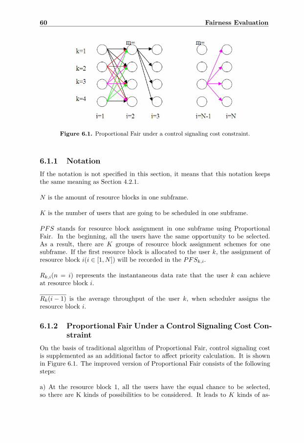
60 Fairness Evaluation
Figure 6.1. Proportional Fair under a control signaling cost constraint.
6.1.1 NotationIf the notation is not specified in this section, it means that this notation keepsthe same meaning as Section 4.2.1.
N is the amount of resource blocks in one subframe.
K is the number of users that are going to be scheduled in one subframe.
PFS stands for resource block assignment in one subframe using ProportionalFair. In the beginning, all the users have the same opportunity to be selected.As a result, there are K groups of resource block assignment schemes for onesubframe. If the first resource block is allocated to the user k, the assignment ofresource block i(i ∈ [1, N ]) will be recorded in the PFSk,i.
Rk,i(n = i) represents the instantaneous data rate that the user k can achieveat resource block i.
Rk(i− 1) is the average throughput of the user k, when scheduler assigns theresource block i.
6.1.2 Proportional Fair Under a Control Signaling Cost Con-straint
On the basis of traditional algorithm of Proportional Fair, control signaling costis supplemented as an additional factor to affect priority calculation. It is shownin Figure 6.1. The improved version of Proportional Fair consists of the followingsteps:
a) At the resource block 1, all the users have the equal chance to be selected,so there are K kinds of possibilities to be considered. It leads to K kinds of as-

6.2 Dynamic Allocation 61
signment S. The user k(k ∈ [1,K]) is assumed to hold the first resource block.The initial value of k is 1.
b) The resource block assignment of the first resource block in the subframe isrecorded in PFSk,1 and Rk(0) is equal to Rk,1(1).
c) At the resource block i(i ∈ [2, N ]), Proportional Fairness is done by assigningresource block i to the user m with the highest priority. The user m is recorded inassignment PFSk,i. The user m with the maximum priority is selected from theusers j(j ∈ [1,K])
mindiv = arg maxj
(Rj,i(i)−Afindiv(Sk,i, Sk,i−1, i)Rj(i− 1)
)
in the individual scheduling map transmission mode and
mbro = arg maxj
(Rj,i(i)−Aρmaxfbro(Sk,i, Sk,i−1, i)Rj(i− 1)
)
in the broadcast scheduling map transmission mode. The second component ofnumerator is the control signaling cost caused by assigning resource block i to theuser j. Rj(i− 1) is the average throughput of the user j, when scheduler assignsthe resource block i. After the completion of allocation of resource block i, itsvalue updates to Rj(i), which depends on Rj(i− 1) and Rj,i(i). It is calculatedby the following formula.
Rj(i) ={
(1− 1tc
)Rj(i− 1) + 1tcRj,i(i), if user j is selected at resource block i
(1− 1tc
)Rj(i− 1), if user j is not selected
where tc is the windows size of average throughput. Here is set to 500. If it is thefirst time to assign resource block to user k for the current subframe, R(k − 1) isassigned with Rk,i(i).
d) Increase k by 1. If k is no bigger than K, then repeat from step b).
e) There are K kinds of resource block assignments PFSk(k ∈ [1,K]). Cal-culate net capacity for each resource block assignment PFSk(k ∈ [1,K]). ThePFSk(k ∈ [1,K]) of the maximum net capacity is optimal assignment S.
6.2 Dynamic AllocationContrast with Proportional Fair, Dynamic Allocation is not only much fairer thanProportional Fair, but also consuming the less computation. It has good perfor-mance for lower signaling cost penalty A. The results will be shown in Section6.4.
The improved version of Dynamic Allocation is implemented by the belowsteps:
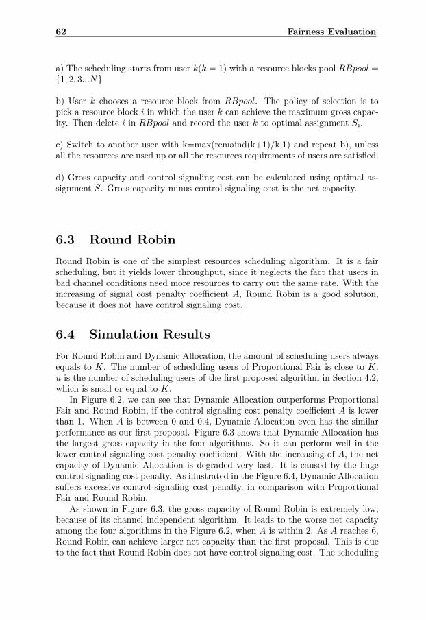
62 Fairness Evaluation
a) The scheduling starts from user k(k = 1) with a resource blocks pool RBpool ={1, 2, 3...N}
b) User k chooses a resource block from RBpool. The policy of selection is topick a resource block i in which the user k can achieve the maximum gross capac-ity. Then delete i in RBpool and record the user k to optimal assignment Si.
c) Switch to another user with k=max(remaind(k+1)/k,1) and repeat b), unlessall the resources are used up or all the resources requirements of users are satisfied.
d) Gross capacity and control signaling cost can be calculated using optimal as-signment S. Gross capacity minus control signaling cost is the net capacity.
6.3 Round RobinRound Robin is one of the simplest resources scheduling algorithm. It is a fairscheduling, but it yields lower throughput, since it neglects the fact that users inbad channel conditions need more resources to carry out the same rate. With theincreasing of signal cost penalty coefficient A, Round Robin is a good solution,because it does not have control signaling cost.
6.4 Simulation ResultsFor Round Robin and Dynamic Allocation, the amount of scheduling users alwaysequals to K. The number of scheduling users of Proportional Fair is close to K.u is the number of scheduling users of the first proposed algorithm in Section 4.2,which is small or equal to K.
In Figure 6.2, we can see that Dynamic Allocation outperforms ProportionalFair and Round Robin, if the control signaling cost penalty coefficient A is lowerthan 1. When A is between 0 and 0.4, Dynamic Allocation even has the similarperformance as our first proposal. Figure 6.3 shows that Dynamic Allocation hasthe largest gross capacity in the four algorithms. So it can perform well in thelower control signaling cost penalty coefficient. With the increasing of A, the netcapacity of Dynamic Allocation is degraded very fast. It is caused by the hugecontrol signaling cost penalty. As illustrated in the Figure 6.4, Dynamic Allocationsuffers excessive control signaling cost penalty, in comparison with ProportionalFair and Round Robin.
As shown in Figure 6.3, the gross capacity of Round Robin is extremely low,because of its channel independent algorithm. It leads to the worse net capacityamong the four algorithms in the Figure 6.2, when A is within 2. As A reaches 6,Round Robin can achieve larger net capacity than the first proposal. This is dueto the fact that Round Robin does not have control signaling cost. The scheduling
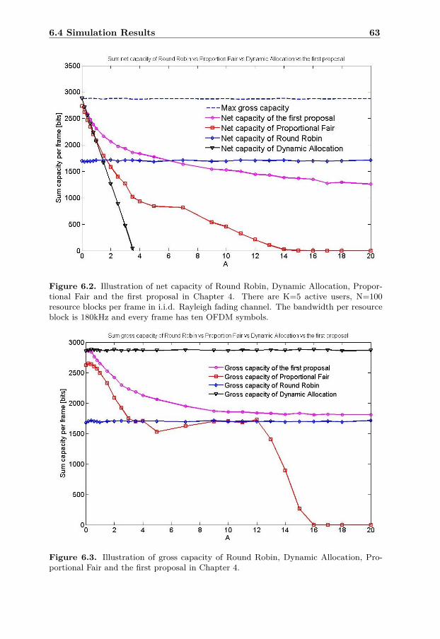
6.4 Simulation Results 63
Figure 6.2. Illustration of net capacity of Round Robin, Dynamic Allocation, Propor-tional Fair and the first proposal in Chapter 4. There are K=5 active users, N=100resource blocks per frame in i.i.d. Rayleigh fading channel. The bandwidth per resourceblock is 180kHz and every frame has ten OFDM symbols.
Figure 6.3. Illustration of gross capacity of Round Robin, Dynamic Allocation, Pro-portional Fair and the first proposal in Chapter 4.
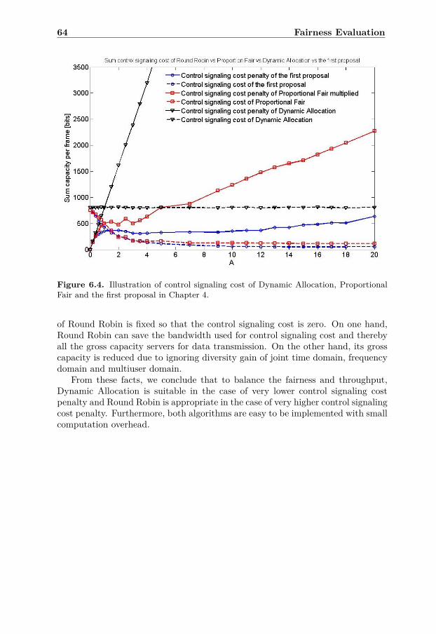
64 Fairness Evaluation
Figure 6.4. Illustration of control signaling cost of Dynamic Allocation, ProportionalFair and the first proposal in Chapter 4.
of Round Robin is fixed so that the control signaling cost is zero. On one hand,Round Robin can save the bandwidth used for control signaling cost and therebyall the gross capacity servers for data transmission. On the other hand, its grosscapacity is reduced due to ignoring diversity gain of joint time domain, frequencydomain and multiuser domain.
From these facts, we conclude that to balance the fairness and throughput,Dynamic Allocation is suitable in the case of very lower control signaling costpenalty and Round Robin is appropriate in the case of very higher control signalingcost penalty. Furthermore, both algorithms are easy to be implemented with smallcomputation overhead.
Chapter 7
Conclusion
This thesis proposes new algorithms for downlink scheduling in LTE/LTE Ad-vanced system. The purposes of the first two proposals are to increase grossthroughput and decrease control signaling cost by finding optimal schedulingscheme so as to maximize the overall net capacity. The third proposal aims atachieving a tradeoff between subframe efficiency and average data rate by seekingan optimal subframe length.
The first proposal demonstrates how to schedule resource blocks under a controlsignaling cost constraint. In this thesis, the channel is modeled as an independentand identically distributed Rayleigh fading channel and the perfect channel stateinformation is assumed at the base station. The gross capacity Gk,n of a particularresource block n for any user k can be estimated with the perfect CSI. The indi-vidual scheduling map transmission and broadcast scheduling map transmissionmodels are proposed to quantize the control signaling cost caused by schedulingmaps. The control signaling cost CSk,n due to assign a particular resource blockn to a certain user k can be evaluated with the proposed models. With the knowl-edge of gross capacity Gk,n and control signaling cost CSk,n, we need to allocateall the resource blocks to the most suitable users in order to maximize the over-all net capacity. A combinatorial problem is formulated and solved via Viterbialgorithm [12] in the first proposal.
By simulations, we find that individual scheduling map transmission modeyields larger net capacity in the case of high control signaling penalty coefficient A,comparing to the broadcast scheduling map transmission mode. Simulation resultsalso show that the net capacity of broadcast scheduling map transmission mode isslightly better, when A is low. In fact, the broadcast scheduling map transmissionmode needs excessive error code to make sure that all the users including theuser with the weakest SNR are able to decode scheduling map correctly, thereforethe net capacity is not really high for broadcast scheduling map transmission.That is the reason why only individual scheduling map transmission is used in thecommercial LTE networks.
The second proposal is derived from the first proposal. It expands the mathe-matic model from two dimensions to three dimensions. Power control is considered
65

66 Conclusion
as the third dimension, in addition to channel condition and control signaling cost.In terms of computation complexity, internal water-filling and external water-fillingmethods are described in the second proposal. The philosophy of external water-filling is to implement water-filling after scheduling as shown in the first proposal.Although external water-filling has no influence on resource blocks assignment S, itstill generates impressive power optimization gain with very low additional compu-tation cost. In contrast with external water-filing, internal water-filling performsbetter, because it considers power control in addition to channel condition of usersand control signaling cost, during the scheduling. However, the disadvantage ofinternal water-filling lies in that it results in heavy computation overhead.
The third scheduling proposal studied in this thesis is adaptive length subframe.The extension of subframe length by adding extra symbols in data region canimprove the subframe efficiency. However, it also leads to the decrease of overallaverage data rate, because the scheduling interval is expanded corresponding tothe extended subframe length and the correlation of Rayleigh fading channel isinversely proportional to the time. The adaptive length subframe is employed torealize a tradeoff between subframe efficiency and average data rate. The optimalsubframe length is found to achieve subframe efficiency as high as possible andmaintain the maximum average data rate at same time. This novel proposal isbeyond the 3GPP LTE standard. However, it can be a potential solution forM2M application in LTE Advanced system and it may be extended in the futureprojects.
In the end, for comparing the fairness of the first proposal, improved versionsof Round Robin, Dynamic Allocation and Proportional Fair are referred. In thecase of very low A, Dynamic Allocation is a good choice for scheduling, sinceDynamic Allocation can produce a large net capacity close to the first proposaland it is one of the fairest algorithms. Under the condition of very high A, RoundRobin is the best algorithm, for the reason that it does not have control signalingoverhead. Furthermore, Dynamic Allocation and Round Robin are relatively easyto be carried out with very small computation overhead. Both algorithms haveobvious limitation and they have extremely poor performance, if A is changed.
Chapter 8
Future Work
From Section 3.2, we learn that the performance of scheduling algorithms for Non-Real-Time is measured by throughput and fairness. The simulation results provedthat the first two proposals can produce a net capacity. However, both algorithmsneglect fairness. As discussed in Chapter 6, if fairness is also taken into account,the mathematic models of the first two proposals need to be recreated and morecomputation overhead has to be brought in scheduling. If the two proposals areintended to be promoted to commercial application, fairness should be one part ofconstraints for scheduling. It will be a four-dimensional mathematic model. Thismodel covers channel condition, control signaling cost, power control and fairness.The most attention should be paid to computation cost. The complexity of thecomputation should remain on a reasonable level, since resource block schedulingmust be done within 1ms.
The three proposals are designed for scheduling Non-Real-Time flows, so thefactor of delay is not considered in this thesis. As mentioned in Section 3.3 andSection 3.4, realistic network must support both Real-Time and Non-Real-Timeflows at the same time. The keys to measure the performance of scheduling algo-rithms for mixture of Real-Time and Non-Real-Time flows are throughput, delayexperience and fairness. The idea of the adaptive length subframe structure inChapter 5 can be borrowed to design a scheduling algorithm for mixture flows. Insuch an approach, the length of subframe is determined not only by channel condi-tion, control signaling cost, maximum Doppler shift but also by delay requirement.The biggest difficulty for the future work is to figure out how to control complexityof the computation of scheduling.
67


Bibliography
[1] 3rd Generation Patnership Project, Technical Specification Group 36.213V8.3.0.
[2] SEVENTH FRAMEWORK PROGRAMME THEME ICT-2009-1.1.
[3] Wikipedia,"2G," http://en.wikipedia.org/wiki/2G, 21 Aug, 2010.
[4] Wikipedia,"3G," http://en.wikipedia.org/wiki/3G, 21 Aug, 2010.
[5] Wikipedia,"4G," http://en.wikipedia.org/wiki/4G, 21 Aug, 2010.
[6] Thales Communications SA "Target Application Scenarios V1.0," 2010.
[7] Matthias Malkowski, Andreas Kemper and Xiaohua Wang, "Performance ofScheduling Algorithms for HSDPA," Second International Conference, Com-munications and Networking in China, 2007.
[8] Seungwan Ryu, Byung-Han Ryu and Hyunhwa Seo, "Wireless Packet Schedul-ing Algorithm for OFDMA System Based on Time-Utility and ChannelState," ETRI Journal. vol. 27, no. 6, pp. 777-787, Dec. 2005.
[9] C.Kalyana Chakravarthy and P.V.G.D. Prasad Reddy, "Modified Queue-based Exponential Rule Scheduler for Improved QOS in OFDMA Systems,"International Journal of UbiComp (IJU), vol.1, no.2, pp. 34-43, April 2010 R.
[10] David Tse and Pramod Viswanath, "Fundamentals of Wireless Communica-tion," Cambridge University Press, 2005.
[11] Erik Dahlman et, "3G Evolution - HSPA and LTE for Mobile Broadband,"Acad. Press, 2008.
[12] Erik G. Larsson, "Optimal Scheduling in OFDMA Under a Control SignalingCost Constraint," IEEE Transactions on Communications, vol. 58, no. 10, pp.2776-2781, Oct. 2010.
[13] Stefan Roth, "Frame Allocation and Scheduling for Relay Networks in theLTE Advanced Standard," Ericsson Research, Beijing, China, 2010.
69

70 Bibliography
[14] Guocong Song, "Utility-Based Resource Allocation and Scheduling in OFDM-Based Wireless Broadband Networks," IEEE Communications Magazine, vol.43, no. 12, pp. 127-135, Dec. 2005.
[15] James Gross, Hans-Florian Geerdes, Holger Karl and Adam Wolisz, "Perfor-mance Analysis of Dynamic OFDMA Systems With Inband Signaling," IEEECommunications Magazine, vol. 24, no. 3, pp. 427-436, March 2006.
[16] Ian Wong and Brian Evans, "Resource Allocation in Multiuser MulticarrierWireless Systems," Springer Press, 2009.
[17] Jim Zyren and Wes McCoy "Overview of the 3GPP Long Term EvolutionPhysical Layer," Freescale Semiconductor, 2007.
[18] Reza Mosssavi, Jonas Eriksson and Erik G. Larsson, "Differential Signalingof Scheduling Information in Wireless Multiple Access Systems," Proceedingsof the IEEE Global Communications Conference, 2010.
[19] Marc Engles, "WIRELESS OFDM SYSTEMS How to Make Them Work?"IMEC, Belgium, Kluwer Academic Publishers, 2002.
[20] R. H. Clarke, "A Statistical Theory of Mobile Radio Reception," Bell SystemsTechnical Journal, vol. 47, no. 6, pp. 957-1000, 1968.
[21] Reza Moosavi and Erik G. Larsson, "Reducing Downlink Signaling Trafficin Wireless Systems Using Mobile-Assisted Scheduling," Proceedings of theIEEE Global Communications Conference, 2010.
[22] Bilal Sadiq, Ritesh Madan and Ashwin Sampath, "Downlink Scheduling forMulticlass Traffic in LTE," EURASIP Journal on Wireless Communicationsand Networking, vol. 2009, Article ID 510617, pp. 18, 2009.
[23] Roger Field, "Research indicates 226 million LTE users by 2015,"http://www.itp.net/580443-research-indicates-226-million-lte-users-by-2015,25 May, 2010.
[24] Sanjay Shakkottai and Alexander L. Stolyar, "Scheduling Algorithm for aMixture of Real-Time and Non-Real-Time Data in HDR," Proceedings of17th International Teletraffic Congress (ITC-17), 2001.
[25] Scott Shen and Chung Ju Chang, "A Cellular Neural Network and Utility-based Scheduler for Multimedia CDMA Cellular Networks," InternationalConference, Wireless Networks, Communications and Mobile Computing, vol.1, pp. 768-773, June 2005.
[26] Kian Chung Beh, Simon Armour and Angela Doufexi, "Joint Time-FrequencyDomain Proportional Fair Scheduler with HARQ for 3GPP LTE Systems," inProc. IEEE Vehicular Technology Conference, pp. 1-5, Oct. 2008.
[27] Hans Jorgen Bang, Torbjorn Ekman and David Gesbert, "A Channel Pre-dictive Proportional Fair Scheduling Algorithm," IEEE 6th Workshop, SignalProcessing Advances in Wireless Communications, pp. 620-624, Sep. 2005.
Bibliography 71
[28] Hang Nguyen, Jerome Brouet, Vinod Kumar and Thierry Lestable, "Com-pression of Associated Signaling for Adaptive Multi-Carrier Systems," Proc.of IEEE 59th Vehicular Technology Conference, vol. 4, pp. 1916-1919, Feb.2004.
[29] Wei Yu and John M. Cioffi, "On Constant Power Water-filling," Proc. IEEEInt. Conf. Communications (ICC), vol. 6, pp. 1665–1669, Helnsinki, Finland,June 2001.
[30] Yahong R. Zheng and Chengshan Xiao, "Improved Models for the Generationof Multiple Uncorrelated Rayleigh Fading Waveforms," IEEE Communica-tions Letters, vol. 6, no. 6, pp. 256-258, Jun. 2002.
[31] Zahid Ghadialy, "OFDM and OFDMA: The Difference," http://3g4g.blogspot.com/2007/06/ofdm-and-ofdma-difference.html, 2010.