1

Modelling of Crushing Operations in the Aggregates Industry

by

Tom Bennett

A thesis submitted to the University of Birmingham for the degree of Master of Research in Chemical Engineering Science

School of Chemical Engineering

University of Birmingham

University of Birmingham Research Archive

e-theses repository This unpublished thesis/dissertation is copyright of the author and/or third parties. The intellectual property rights of the author or third parties in respect of this work are as defined by The Copyright Designs and Patents Act 1988 or as modified by any successor legislation. Any use made of information contained in this thesis/dissertation must be in accordance with that legislation and must be properly acknowledged. Further distribution or reproduction in any format is prohibited without the permission of the copyright holder.

2

Abstract

The aggregate industry is a very important part of the UK economy. Aggregates are used in a variety of different applications from rail ballast to building material. It is therefore important that the production of aggregates is as efficient and cost effective as possible.

This MRes research project was based at the School of Chemical Engineering at the University of Birmingham. The software package JKSimMet was used to model processes at MountSorrel Granite quarry in Leicestershire. The project aimed to show whether there were functional relationshipsbetween the input data in the primary crushing phase (gap size (mm), feed size distribution, throughput (t/hr) and ore type) with the output data (product size distribution and power draw).

The effect that changing the gap size has on the product size distribution was investigated for the gyratory crusher using the software package JKSimMet. Various simulations were run so that product size distributions were given for different values of CSS (close side setting). The percentage of granite passing various sizes in the product size distribution was plotted against the gap size using Matlab. Using the curve fitting software package GnuPlot, functions were ascertained that fit the data from JKSimMet. It was found that these functions were based on the Rosin-Rammler distribution for large enough values of CSS.

The effect of changing the feed size distribution was investigated for the gyratory crusher. The feed size distributions were generated artificially using the Rosin-Rammler distribution on Matlab. It was found that feed size distribution has a direct effect on product size distribution on JKSimMet but the relationship was not a smooth one as between gap size and product size distribution. There was no real relationship between feed size distribution and power draw.

Changing the throughput of the gyratory and cone crusher was investigated using JKSimMet. It was found that the throughput has no effect on the product size distribution on JKSimMet as is consistent with the literature, but did have a linear effect on the power draw.

The ore type has no effect in the primary crushing stage, but a large effect in the blasting phase, so using the Kuz-Ram distribution a different feed size distribution was used to represent each ore type from the same blasting conditions.

It was shown that there is a relationship between the value of the constant representing the ore type in the Kuznetsov equation and the value of d50 in the product size distribution of the gyratory crusher. This shows that the blasting phase has a measurable effect on the product of the primary crusher.

3

Acknowledgements

I would like to express my gratitude to my supervisor Dr Neil Rowson and to my secondary supervisor Dr Phil Robbins from the School of Chemical Engineering at the University of Birmingham for all of the help and guidance that they have given me during this project and for the seemingly endless patience that they have both shown whenever I made mistakes or got stuck. Thanks also to Dr Richard Greenwood from the University of Birmingham for the help he has given me during the year. I would also like to thank Jon Aumônier, from MIRO for his help and support throughout the year. Sincere thanks also go to the European Union and MIRO for providing me with the funding to carry out this research project.

4

Contents

Chapter 1: Introduction 9

Project Objectives

Chapter 2: Fracture Mechanics and Granite Properties 11

X-Ray Fluorescence Drop Weight Testing Laws of Comminution Granite Microstructure Comminution of Granite

Chapter 3: Mountsorrel Granite Quarry 23

Chapter 4: Review of Comminution Simulation Software 24

USimPac JKSimMet Comparitive Review Between UsimPac and JKSimMet

Chapter 5: Modelling of the Blasting Process 34

Definitions Blast Hole Design Kuz-Ram Model of Blasting

Chapter 6: Previous Models of Crushing Processes 39

Whiten Crusher Model Uses

Chapter 7: Changing Gap Size 43

Procedure Results and Discussion

Chapter 8: Changing Feed Size Distribution 49

Procedure Results and Discussion

5

Chapter 9: Changing Throughput 53

Procedure Results and Discussion

Chapter 10: Changing Ore Type 56

Procedure Results and Discussion

Chapter 11: Conclusions 62

Future Work

References 64

Appendix 1: Matlab Codes 66

Appendix 2: JKSimMet Flowsheets 81

Appendix 3: Appearance Functions for Different Ore Types 83

Appendix 4: Size Distributions for Gyratory Crusher 85

6

Table of Figures

Figure 1: Schematic of equipment used for X-Ray Fluorescence. 12

Figure 2: XRF spectrum for Mountsorrel granite 15

Figure 3: Schematic of a drop weight testing machine. 16

Figure 4: Image showing grain boundary between a region of quartz and a region of K-

feldspar in a granite. 18

Figure 5: Mechanisms of the propogation of a fracture in a material . 18

Figure 6: Image showing differences between different types of porosity. 19

Figure 7: JKSimMet flowsheet for Mountsorrel granite quarry 25

Figure 8: JKSimMet screen shot. Unit processes selected from drop down box and

placed on screen. 26

Figure 9: JKSimMet screen shot. Add solids handling and stockpiles. 27

Figure 10: JKSimMet screen shot. Input the flow rates to crusher. 28

Figure 11: JKSimMet screen shot. Input particle distribution to the crusher. 28

Figure 12: JKSimMet screen shot. Setting the crusher parameters. 29

Figure 13: JKSimMet screen shot. Enter drop weight test data from granite. 30

Figure 14: JKSimMet screen shot. Data on the power draw and crusher energy

is entered. 31

Figure 15: JKSimMet screen shot. Comparison of plant and JKSimMet

generated data. 32

Figure 16: Diagram to illustrate decking in blastholes. 36

Figure 17: Cross section of a gyratory crusher. 40

Figure 18: Cross section of a jaw crusher. 40

Figure 19: Simple flowsheet diagram for crushing process. 41

Figure 20: Plot showing how the percentage of rock passing 50 mm

changes with gap size. 45

Figure 21: Plot showing percentage of rock in feed size distribution

from gyratory crusher passing sizes from 10 mm to 90 mm. 46

Figure 22: Plot showing data points of percentage of rock bigger than 50 mm

with chaging gap size with curve fitted to data points by Gnuplot. 47

Figure 23: Values of constants in equation 20 changing with d values. 48

7

Figure 24: Plot of the artificial particle size distributions generated using

log normal distribution and a Rosin–Rammler distribution 50

Figure 25: Plot showing how d values change in feed size distribution

with changing d80 in the feed size distribution. 52

Figure 26: Power Draw plotted against throughput. 54

Figure 27: Pendulum Power plotted against throughput. 54

Figure 28: Plot of the product size distributions for different rock types

from Gyratory crusher. 57

Figure 29: Plot of the power Draw of gyratory crusher compared to

d50 value for each ore type. 58

Figure 30: Plot of Kuz-Ram distribution generated in Matlab. 60

Figure 31: Plot of d50 of product size distribution varying with parameter

A in Kuznetsov equation. 61

8

List of Tables

Table 1: Elemental analysis of different types of granite from paper by El-Taher. 14 Table 2: Rock fracture data for Barrasford basalt generated by drop weight

testing. 17 Table 3: Rock fracture data for Mountsorrel granite generated by drop weight

testing. 17 Table 4: Example of simulation of a product size distribution for CSS value of 100 mm

produced JKSimMet. 44 Table 5: Constant values in equation modelling how d values vary with

gap size. 48 Table 6: Example of an artificial product size distribution produced on Matlab

using Rosin-Rammler equation with a d80 value of 160 mm. 51 Table 7: Power draw values and pendulum power for different values of

throughput in a gyratory crusher. 53 Table 8: Data for power draw and d50 values for different ore types

on JKSimMet. 57 Table 9: Parameters used in the Kuz-Ram distribution 59

9

Chapter 1: Introduction

1.1 Scope of project

This MRes thesis is part of an EU funded study in Energy Reduction in aggregate quarry operations. (EE Quarry). The overall aim of the European partners is to monitor and reduce energy wastage and create more environmental friendly quarry operations. Two major issues in quarry operations are:

1. Energy Wastage due to inefficient flowsheet development of the quarry processing operations

2. Generation of fines from crushing (nominally -4 mm) which cannot be utilised and sold. These sometimes have to be stored and stockpiled on site. This represents a waste of energy due to over crushing and costs money in terms of storage space and environmental control.

This thesis looks at the possibility of producing an easy to operate simulator for plant operators which can predict plant crushing behaviour in primary crushers. Data generated from this may allow operators to gain better control of the plant, reducing the generation of minus 4 mm material. It would also act as a training tool- allowing non graduate operators to better understand key variables(e.g. Crusher gap setting) in the mineral processing of aggregate products ( in this case granite from MountSorrel Quarry).

1.2 UK Aggregate Industry

The aggregate industry is worth £3 billion per annum to the UK economy (Lafarge Aggregates 2006).This study will centre on granite production at MountSorrel Quarry owned by Lafarge/Tarmac.Granite aggregates are used extensively in a number of applications including use on roads, use as rail ballast and also as a building material. The physical properties of granite such as its hardness and chemical inertness are conducive to it being used in this way as a filler in civil engineering operations.

1.3 Efficient Plant Operations

It is therefore important that the production of this aggregate is as efficient as possible in terms of energy consumption and particle size distribution to meet the customers’ specification. Key to this is the elimination of unwanted fines during comminution processes on site. Fines are defined as being particles smaller than a certain diameter (4 mm) in the Mine-to-Mill Process Report produced by Tarmac Limited and Partners (2011), they are valueless and cannot be sold-hence they are stockpiled on site creating space and environmental issues. All fines that are produced are a potential waste of comminution energy and cost money to Lafarge/Tarmac the MountSorrel operating company. It is therefore important to try and reduce the amount of fines that are produced and optimise the whole comminution process. A relatively small percentage reduction in the amount of fines produced can result in a large financial gain over time due to the size of the industry (In terms of annual production rates from Europe’s largest granite quarry). There is also the question of energy use, the aggregates industry uses a significant proportion of the total energy consumed in the UK. So decreasing energy use by a relatively small amount (1 or 2%) will also result in a large saving in

10

operating costs per annum. This is particularly relevant as granite aggregate is a low cost product per tonne and profit margins are small for Lafarge/Tarmac in a very competitive marketplace that is often controlled by transport costs.

1.4 Research Project Objectives

The ultimate aim of this 120 credit MRes research project carried out in the School of Chemical Engineering at the University of Birmingham is to begin the development of a spreadsheet based simulation package that is easy to use and understand at the user interface, the ultimate aim is to test this at MountSorrel quarry.

It is hoped to start to understand the functional relationships between input and output data from JKSimMet, a modelling package that has previously been used to predict crusher performance at Mountsorrel. It will be useful to be able to quantify how changing one of the inputs (such as crusher throughput (tonnes per hour of granite), crusher open gap setting (mm) and rock hardness (defined by drop weight testing)) will affect the resulting size distribution for each of the crushing unit processes on site.

This increased understanding will hopefully help the plant operators to reduce the amount of fines produced and also to optimise the energy consumption per tonne of saleable granite produced. It will be useful to see whether the functional relationships that we find from JKSimMet will match functional relationships that are found from experimental data that has been produced from an onsite sampling campaign, this will hopefully add more evidence that JKSimMet is generally an accurate software package for quarry aggregate production applications that can be used in place of expensive experiments and real time plant modifications that will affect plant production due to plant downtime.

The ultimate aim of the EE Quarry project is to combine all quarry site operations (haulage, blasting,mineral processing, drying, screening) into one functional package that is easy to use by plant operators (that are not trained engineers) .This MRes project is a small part of this process and will link into parallel studies being carried out in Poland, the UK, Spain and Greece.

11

Chapter 2: Fracture Mechanics and Properties of Granite

For comminution processes to be as efficient and profitable as possible it is important to understand how the rock that is being processed will behave under an applied force so that the various stages of the comminution process can be designed to be as efficient as possible. There are a number of techniques that can be used to measure physical properties of granite and some of these are described in the following section. The drop weight test in particular is very important in that it gives the kinetic energy required to fracture the rock and also the size distribution of the resulting fragments of the granite when subjected to an impact force.

2.1 X-Ray Fluorescence

X-ray fluorescence is a non destructive measurement technique that is used to measure the elemental composition of a sample. It can be used on solids in powder form and also used on liquids. This technique makes use of X-rays which are a form of electromagnetic radiation at the high energy end of the electromagnetic spectrum. The wavelength of an X-ray is typically somewhere between 0.01nm and 10nm. Any lower than this and the radiation would be at the gamma end of the spectrum.

The basic procedure is that an X-ray is shone onto the sample that to be measured. The fluorescent X-rays that are emitted from the sample are detected and the energy or wavelength can be measured depending on whether the technique being used is energy dispersive X-ray fluorescence or wavelength dispersive X-ray fluorescence (hereafter referred to as EDXF and WDXF respectively).

An electric current is passed through a filament; this causes electrons to be emitted. These electrons are then accelerated by a potential difference towards an anode. When the electrons hit the anode they decelerate causing them to lose energy which is emitted as X-ray radiation. These X-rays are then shone out of a thin window made of beryllium, and towards the sample.

This technique involves the use of the photoelectric effect. When an X-ray is shone onto the sample, a photon will be absorbed by an electron in the sample, the energy from the absorbed photon will either cause the electron to jump up to a higher energy level or, if the X-ray has a high enough frequency, the electron will have enough kinetic energy to completely leave the atom. This will cause a gap to have appeared in one of the electron shells of the atom that will then be filled by an electron jumping down from a higher energy level. When this happens this electron will emit a photon of energy (of different frequency to the source X-ray). This photon can then be detected and the energy or wavelength measured. Each element has unique energy levels, so the energies of the X-rays that are emitted for electrons jumping down an energy level will be unique for each element. Each element has its own fingerprint, so the element can be easily identified by the frequencies of the X-rays that are emitted.

For an electron to be emitted from an inner shell the photon of energy that it absorbs has to have energy greater than the work function of that electron. This work function is the binding energy between the electron and the nucleus of the atom. The energy of a photon is given by Plank’s Law:

E = hf (1)

12

where E is the energy of the photon, f is the frequency of the electromagnetic radiation and h is Plank’s constant. Therefore the energy of a photon is proportional to the frequency; this means that for the energy of the photon to be higher than the work function it has to have a high frequency. This is why X-rays have to be used for this measuring technique and why lower frequency electromagnetic radiation like visible light cannot be used. It is however, important that the energy of the X-ray is not too high. If it is too high then the photon will not bind with the electron, it will not be absorbed and will just pass through the sample. Therefore it is best if the energy of the X-ray is just above the work function energy. This is difficult if the sample has many different elements in it all with different work functions. The fluorescence yield is defined as the intensity of the fluorescent X-rays over the intensity of the incident X-ray. Figure 1 shows a schematic of an X-Ray Fluorescence wavelength dispersive unit.

Figure 1: Schematic of equipment used for X-ray fluorescence, specifically the wave-length dispersive technique (http://archaeometry.missouri.edu/xrf_overview.html)

The differences between wavelength dispersive and energy dispersive X-ray fluorescence are mainly in how the fluorescent X-rays are detected. In the EDXF technique the energies of the fluorescent X-rays are measured directly. The X-rays hit the detector and are absorbed by it; this then causes electron-hole pairs to form. The number of these pairs that form is equal to the energy of the fluorescent X-ray over the fixed energy needed to form an electron-hole pair for the detector material. The resulting current of electrons is proportional to the number of electron-hole pairs that have been formed so the energy of the fluorescent X-ray can be directly calculated from the resulting current. This analysis is repeated at a very high rate, the calculated energies are presented as energy channels on a graph.

The WDXF method uses a crystal to diffract the fluorescent X-rays. This will occur according to Bragg’s Law. The Fluorescent X-rays will be diffracted at slightly different angles according to their wavelengths, and the detector will be placed at a known angle to the crystal so that all the X-rays detected at that point will have a specific wavelength. The detector can then be moved through the different angles to the crystal and the X-rays at each wavelength can then be easily detected. The spectrum of the fluorescent X-rays can then be gradually built up. A schematic of the equipment for

13

WDXF is given in figure 1, which has been taken from the University of Missouri Research Centre website.

There are a number of advantages and disadvantages that the EDXF and the WDXF have over each other. The main advantage that the WDXF technique has is that it can provide a much higher resolution than the EDXF technique. This makes it easier for samples that are quite complicated in their elemental composition to be analysed more precisely. However the EDXF technique is more efficient than the WDXF, this is because of the diffraction of the X-rays by a crystal in the WDXF technique. Another difference is that the WDXF technique is clearly going to be a much more time consuming technique than EDXF. This is because in EDXF the spectral lines are known almost instantly but in WDXF the spectral picture has to be built one wavelength at a time, unless we have multiple detectors which will be very expensive.

An advantage of the XF measurement technique is that it can be used for a very quick qualitative analysis; it can tell us the elements that are contained in a sample very quickly. However it is difficult to use this technique to detect the very lightest elements. Lithium, helium and hydrogen cannot be easily detected, but all elements heavier than this right up to uranium can be easily detected.

A disadvantage of the technique is how easy it is to interpret the results incorrectly. This is because not all the X-rays that are detected will be fluorescent X-rays, some of the incident rays will not have been absorbed by the sample or even have passed through it. Some of the X-rays will have been scattered by Compton scattering and if these are detected and thought to be fluorescent X-rays it will seriously skew the results. These results will give erroneous spectral peaks which will not tell us anything about the elemental composition of the sample but could in fact make it appear that there are elements in the sample that are not there at all. Another factor that requires care to be taken is the fact that some elements in the sample can interact with each other. A fluorescent X-ray emitted by one element might be of high enough energy to be absorbed by another element in the sample, thereby removing the original fluorescent X-ray from the results and making the peak height for that element lower than it should be, and making the peak height for the second element higher than it should be.

Another disadvantage of this technique is the fact that it cannot detect the differences between different isotopes of an element. An isotope will have the same number of protons in the nucleus and electrons in the outer shell, but will have a different number of neutrons in the nucleus. As this technique utilises the fluorescent X-rays that are emitted from electrons orbiting the nucleus, it cannot detect the number of neutrons in the atom. If this information is required other techniques have to be used (normally mass spectrometry, which will not be discussed here). This technique also cannot detect the ionisation state of an element, it cannot detect whether the element has the same number of electrons as it has protons or not. This also has to be done by other techniques.

This technique is relevant to the aggregates industry. It is important when mining an ore that the elemental composition is known, it is important to know whether any rare trace elements are to be found in the area of interest. Granite can also be a source of valuable by-product minerals. This technique therefore aids understanding as to what the value of the granite that is being quarried may be in terms of trace metals.

14

The preparation of the sample is a very important part of the procedure. How well the sample isprepared will affect the accuracy of the final results. For the rock analysed from Mountsorrel quarry this involved crushing the granite to a powder, mixing with a wax and pressing it into a pellet with a pressure of 20 tons for approximately 20 s.

Composition (ppm) Wadi Allaqi Ibrahim Gebel Pacha El-Shelal Syhail Island

Al2O3 96,500 93,000 91,500 11,100

CaO 40,500 14,500 6500 7500

Fe2O3 110,000 30,500 11,000 12,000

K2O 46,850 29,400 46,550 50,050

MgO 11,500 3000 500 500

MnO 1510 430 2450 760

Na2O 14,500 1500 13,500 20,500

P2O5 7250 1400 550 700

SiO2 594,000 462,000 551,500 585,500

TiO2 17800 4150 1800 1200

F 1500 1000 1000 1000

S 130 90 795 350

Ba 1053 711 142 253

Cl 74 11.5 14.5 13

Co 42 4 ‒ ‒

Cr 91 49 44 38.5

Cu 19 14.5 13.5 14.5

Mo 3.5 3.5 2.5 1.5

Ni 9 7 6.5 8

Pb 12.5 11.5 16.5 19.5

Se 2 ‒ 1 ‒

Sn ‒ ‒ 1 9

Sr 352 132 34 37

Ti 0.1 0.2 0.55 0.55

V 139 22 7 14.5

Zn 128 47 23.5 30.5

Table 1: Elemental Composition of Different types of Granite in parts per million(El-Taher, 2012).

An example of XRF being used to determine the chemical composition of granite is shown in Table 1 (El-Taher, 2012). The four samples of Egyptian granite are seen to have slightly different chemical compositions. The El-Shalal and Seyhel Island are older granites and the El-Allaqi and Geble Ibrahim Pasha are younger granites. These results from El-Taher show that the elemental composition of granite samples vary according to where the samples were taken from. But Si and Al compounds are most abundant in all four samples. However interesting element concentrations of Ti, Mg, V and Zn occur in some of the Egyptian Granite analysed.

Data generated from XRF analysis of Mountsorrel granite are shown in figure (2).

15

Figure 2: XRF spectrum for Mountsorrel granite (Ruszala 2012)

2.2 Determining Granite Rock Fracture Parameters: Drop Weight Testing

A drop weight test has been designed by JKRMC (the Julius Kruttschnitt Mineral Research Centre) to give the breakage characteristics of the rock that can be fed into their simulation packages for primary crushing. It is based on an equation that has been used in a number of papers including Bearman et al. (1996)

t10 = A(1 – e-bEcs) (2)

where t10 is the percentage of rock passing a tenth of the original size, Ecs is the specific breakage energy of the rock and A and b are ore specific characteristics. This equation was proposed by Leung in 1987. From this equation a matrix is created with values of t2, t4, t25, t50 and t75 entered against different values of t10. This information is also given by Hosseinzadeh et al. (2012)

For the drop weight test, a known mass is dropped onto a sample from a known height. The potential energy of the drop weight and then the kinetic energy can be determined from the mass of the weight. The drop weight unit itself is an empty frame that has a mass of around 3kg. Extra weights can be added inside the frame. There is a removable cover plate that can be unscrewed when adding or removing weights from the drop weight. When the required number of weights is inside the drop weight, the cover plates are then bolted back on to the back and the front of the drop weight to ensure that they do not fall out when a test is being carried out. See figure 3 for a schematic of a drop weight tester.

16

The kinetic energy that the weight has when it hits the sample can be very easily calculated by the principle of conservation of energy as the difference between the gravitational potential energies of the weight at the height it is dropped from and when it is resting on top of the sample. This is therefore:

E = mg(hi – hf) (3)

Where m is the mass of the weight, g is acceleration due to gravity and the two h values are the heights of the weight initially and at the end of the test respectively. The kinetic energy of the weight at which the rock fractured can therefore be calculated using the height at which the weight was dropped from that caused the rock to fracture. The velocity at which the drop weight will impact the sample can also be estimated by comparing the kinetic energy with the initial potential energy.

Figure 3: Typical Schematic of drop weight testing machine. (Sabih. A. et al. 2012)

The velocity will be given by the equation:

V = (2g(hi – hf))1/2 (4)

Where all the symbols are the same as in the previous equation.

When the sample has fractured it can then be screened so that the fractured rock can be collected into its different size brackets. The percentage of the sample that has fractured into a size smaller than a certain percentage of the size of the original sample can then be measured.

One of the main disadvantages of the drop weight test is that it does not allow the fraction of the energy from the dropped weight that is actually needed to fracture the rock to be calculated. This is called the comminution energy. The efficiency of energy transfer will be different for different materials, if we want to calculate the comminution energy then we could use the pendulum test. However this is a much less flexible test than the drop weight test.

When the results of drop weight tests on Mountsorrel granite and on Basalt from Barrasford were compared it was found that the Mountsorrel granite had a slightly lower value of t75 than Barrasfordbasalt. The rock fracture data for Barrasford basalt and Mountsorrel granite are given in table 2 and

17

table 3 respectively (Ruszala, 2012). Mountsorrel granite is a very hard rock which behaves similarly to basalt in primary crushing operations. This has been confirmed by plant operators.

Table 2: Rock fracture data for Barrasford basalt generated by drop weight testing (Ruszala, 2012)

Table 3: Drop weight test results for Mountsorrel granite (Ruszala, 2012)

2.3 Microstructure

Granite has certain properties that make it useful in the aggregates industry, and these influence how it may be mined and quarried. One of the most important properties is the grain size. Grain boundaries have an effect on the stress required for breakage of the rock and will define the behaviour of the granite during processing.

Griffith (1924) proposed that the failure of a brittle solid under an external force is caused by cracks that were already in the material, the energy would be absorbed by the new crack surface. Fragmentation occurs when the external work done on the solid is greater than the potential energy of the new crack surface. This theory was based on work done by Inglis (1913), who by looking at an elliptical hole in an infinite plane found that the stress concentrated at the tips of the ellipse was proportional to the radius of the ellipse and the size of the ellipse. Griffith then applied this theory to cracks in a brittle solid, by considering them in the same way. By doing this he managed to define a relationship between the stress required for fracture and the length of a crack in the solid. The compressive stress that is required for fracture as given by Griffith is:

≥ 8 2 (5)

Where σ is the compressive stress for fracture, E is the Young’s Modulus, α is the surface energy per unit area of the crack surfaces and c is the crack half length.

The strength of granite is seen to decrease with increasing grain size as is shown by equation 5. The greater the crack length, the lower the stress required for fracture initiation. It has been suggested

18

that longer grain boundaries give longer paths of weakness, which cracks can propagate along more easily. This would mean that the strength of the rock would decrease. It was also shown however that crack initiation does not really change with increasing grain size, but the Young’s modulus does decrease with increasing grain size. Granite therefore fractures under smaller loads for larger grain sizes. Hence the grain size of the granite (determined by its geological history) is a key factor in defining its performance as an aggregate.

Figure 4: Image showing grain boundary between a region of quartz and a region of K-feldspar in a granite (Eberhardt et al 1999)

As shown in figure 4, taken from the paper by E.Eberhardt et al (1999), the grain size in granite can be of the order of hundreds of micrometers to millimetres. The grain size has been stated as typically being between 0.5 to 3 mm by Chaki et al (2008). In their paper on the influence of thermal damage on physical properties of a granite rock. The grain size will be determined at the time of genesis of the granite by the cooling time of the ore body. In simplistic terms the faster the cooling rate the greater the finer the resultant grain size. The grain boundaries are the areas where the granite is weakest and most likely to break under mechanical stress. Cracks can propogate in different ways, this is discussed in the paper by Chang et al (2002). The three different modes of crack propogation are: the tensile opening mode, in which the crack faces pull away from each other in a direction perpendicular to the crack, plane sliding mode, in which the two faces slide across each other in the direction of the crack and the out of plane mode where the crack faces slide across each other parallel to the front of the crack. These mechanisms are shown in figure 5.

Figure 5: Mechanisms of the propogation of a fracture in a material (Chang et al. 2002)

19

2.4 Porosity of Granite

The total porosity of a solid is simply defined to be the ratio between the volume of the void space inside the rock over the total volume of the rock, typical values of porosity for granite are found to have been 0.36% and 0.52% as given by Chaki et al. (2008) which is also confirmed by David et al. (1999). This was found by measuring the mass of the granite when dry and then measuring again when the granite was saturated with water, using the density of water the porosity could be calculated from the ratio between these two masses. There are also other defined other measures of porosity, such as open porosity, where only the proportion of the pores that are in contact with the surface of the granite are considered, the connected porosity considers void space that is fully interconnected between two opposite ends of the sample. These porositys are all shown and labelled on figure 6 which was taken from the paper by Chaki et al (2008). Typical pore sizes in granite tend to be in the order of micrometres, a typical pore size distribution for granite is given in the paper by Lindqvist et al. (2012) and the vast majority of the pore sizes are less than 150 μm2 in area.

Figure 6: Image showing differences between different types of porosity (Chaki et al. 2008)

The porosity was shown to have a clear impact on the compressive strength of granite by Ludvico-Marques et al. (2012). The more porous the rock, the lower the compressive strength. It has also been shown by Hu et al. (2011) that the smaller the pore size on the surface of granite aggregate, the easier it is for water to be absorbed. The average pore diameter was also shown to have a greater effect on the rate of water absorbtion that the overall porosity. As the granite breaks more easily when saturated with water we can say that if the average pore size on the surface of the granite is smaller, then it will be easier to break the granite when it is wet.

20

2.6 Microcracks in Granite

Micro cracks in rock have been split into 4 different types:

Grain boundary cracks Intragranular cracks (cracks totally contained within a single grain not extending to a grain

boundary) Intergranular cracks (cracks extending from a grain boundary into a grain) Multigranular cracks (cracks across multiple different grains and boundaries)

In crystalline materials it is expected that the most flaws will be grain boundary cracks, so in granite it will be expected that most micro cracks will be along the grain boundaries. However it has been observed from experiment that intragranular cracks also occur in some weaker mineral constituents such as feldspar (especially weathered feldspar).

The geological history of the granite and the blasting history of the granite will control the nature of the microcracks in the ore being processed. Hence this will determine how the granite fractures in the primary and secondary crushing operations and the particle size distributions produced during comminution. The relationship between blasting and primary crushing is key to efficient plant operations by control the particle size distribution entering the primary crushing ,however blasting can also effect the microcracks in the granite and this will effect the crusher performance and energy consumption. It is an overall aim of the EE Quarry project to link these two separate processes together in a common model to better predict (and reduce) energy usage in quarries.

The three laws of comminution that were proposed by Bond, Kick and Von Rittinger are now to be discussed in more detail, and the applicability and accuracy of each of these laws will be considered in turn, as each law has been found to be applicable for different size ranges and therefore different phases in the mine-to-mill operation. The three laws of comminution are given in detail in Donovans Thesis (2003).

The Von Rittinger law is based on the assumption that the energy required to break a particle is dependent on the surface area of the particle before and after it is crushed. So finer particles will take more energy to fragment than coarser particles. The Von Rittinger law is given as follows:

E = K(A2 – A1) (6)

Where E is the breakage energy, A1 is the specific surface area of the particle before fragmentation, A2 is the specific surface area of the final particle after fragmentation and K is a constant. This law can also be expressed in terms of particle diameter as specific surface area is inversely proportional to the particle diameter:

E = K( 1d2 − 1

d1) (7)

Where d1 and d2 are the diameters of the initial and final particles respectively. It has been seen that the Von Rittinger law is more applicable to the fragmentation of finer particles, this is because volume does not have such a large effect for fine particles and the Von Rittinger law does not take volume into account, only surface area.

21

The Kick law assumes that the energy to fragment particle is proportional to the volume of a particle. It is given as follows:

E = K(ln(d1/d2) (8)

where all the symbols are the same as before.

However it does not work very well for the reduction in size of fine particles. This is because it is dependent entirely on the ratio between the volume of the particle before it is fragmented and after it is fragmented, so two fragmentation processes could cause a decrease in volume by the same amount, and it would be predicted that this would require exactly the same fragmentation energy by Kick’s law. However it has been clearly observed that fracturing finer particles requires more energy. Kick’s law does not take this into account.

The Bond law considers the surface area and the volume of the particle. This law was empirically derived by a series of grinding tests. This equation is applicable for finer particles than for Kick’s law and coarser particles than for Von Rittinger’s law. This equation has been modified for use as modelling the power draw of size reduction equipment. It was found that it works reasonably well for grinding and milling processes but not very well for primary crushing. The Bond law is as follows:

= 1 − 1

(9)

again with all symbols the same as before.

It has been suggested by Gongbo et al. (1992) that these three laws of comminution can be combined into one general differential equation using fractal theory. This equation (10) is given below:

dE = -Kdx/xn (10)

with the value n being a different constant for each of the three laws, 2 for the Von Rittinger equation, 2.5 for the Bond equation and 1 for the Kick equation. It can be seen that integrating the above equation with each value of n gives the Von Rittinger, Bond and Kick equations respectively.

However it was proposed that this equation is not valid as a general of comminution, but should be modified in the following way:

dE = -Kdx/xf(x) (11)

where f(x) is a function of the particle fineness. Fractal theory was used to define the function f(x) in the above equation. The concept of fractal dimension was first used to describe structures that were self-similar (i.e. that would have the same appearance no matter how much the structure was magnified.) A fragment of rock cannot be described as a fractal in a mathematical sense, but it can be seen as being statistically self similar, so therefore can be given an approximate fractal dimension.

It was then shown by Gongbo et al. that the comminution equation could be written as:

dE = -Kdx/x4-Ds (12)

22

where Ds is the Fractal dimension. This equation agreed well with experimental observation.

2.7 Effect of Fracture Mechanics of Rock Behaviour

For comminution processes, the characteristics of the rock that is to be mined are very important so that it can be processed as efficiently as possible. As the aim of the comminution process is to break the rock down into a specific size range the most significant characteristic of the rock is how it will break under a load. It is desirable to be able to find a relationship between the energy applied to breaking the rock and the size of the resultant fragments. There are a number of parameters that can be measured and that should have a bearing on the comminution process. These are listed below and are taken from the paper by Bearman et al. (1997)

Specific Gravity Uniaxal Compressive Strength Point Load Strength * Poisson's Ratio * Schmidt Rebound Hardness * Aggregate Impact Value (AIV) * Bulk Modulus * Water Absorption Fracture Toughness Brazilian Tensile Strength Young's Modulus (static and dynamic) P & S wave velocity Aggregate Crushing Value (ACV) 10% Fines Modulus of Rigidity

It was found that the most important characteristics were the fracture toughness, the Brazilian tensile strength and the point load strength. Bearman et al. used experiments to show a correlation between fracture toughness and the ore breakage parameters A and b in the equation for t10 from drop weight testing. This meant that the value of t10 could be estimated for a given energy input per unit mass. Therefore the breakage behaviour of the rock can be modelled if the energy input per unit mass is known.

It has been observed by Kujundzic et al. (2008) that changing the ore type has only a very minor effect on the specific energy of crushing in a jaw crusher. It was suggested that the reason behind this is that there is a different mechanism used for crushing in a jaw crusher than used by a hydraulic hammer. Impact is the main mechanism for a hydraulic hammer, whereas in a jaw crusher the rock is crushed by being ground against the liner of the crusher chamber and the surface of the other rocks in the crusher by the repeated motion of the crusher. As a gyratory crusher works by a similar mechanism to a jaw crusher we can expect that this will be the result for the gyratory crusher on JKSimMet.

23

Chapter 3: Mount Sorrel Granite Quarry (Operated by Tarmac/Lafarge)

At Mountsorrel Granite Quarry Leicestershire a gyratory crusher is used for the primary crushing of the granite extracted after blasting from the quarry. Cone crushers are utilised for the secondary crushing. Various screens are also used to size the granite into stock-piles of controlled size range for shipments.

Lasers are used to find the best places in the rock to place the explosives, this is carried out to minimise the vibration and the noise produced by the blasting operations as the site is situated close to the village of MountSorrel in Leicestershire. Two pneumatic drills then bore holes that are 110mm in diameter and 18 metres deep. A controlled dosage of explosive charge is then placed in theholes and a carefully coordinated blast (in terms of detonation sequence) will take place at 12.30 pmon week days. The blast produces a pile of rock on the floor of the quarry that will have a mass of between 20,000 and 30,000 tonnes. This can then be picked off the floor by the large excavator. At Mountsorrel the excavator has a bucket capacity of 280 tonnes. The blasting has been carefully designed so that the granite boulders produced will be small enough for the primary crusher, but some will still be too large. At this point these a large manganese steel ball is dropped onto these larger rocks to break them up. The rock is then driven up to the primary crusher in large trucks.

The primary crusher used at Mountsorrel quarry is a gyratory crusher, a Nordberg 6104. Approximately 3000 tonnes of rock per hour are crushed by the primary crusher. After this stage the resulting rock is passed over a screen where products under 30 mm in diameter are screened out, this is because particles below this size do not need secondary crushing (as this would generate extra fines). Granite particles coarser than 30 mm are transported to a pile called the ‘Surgepile’ with a capacity of 140,000 tonnes.

The granite rock is carried by conveyor belt from the Surgepile to the secondary crushing stage. At Mountsorrel there are three cone crushers that are used for secondary, tertiary and quaternary crushing. After secondary crushing the granite is passed through 12 vibrating screens which separate all of the crushed rock into 9 different size groups. The rock in these different groups can be used then for different applications such as rail ballast, cement aggregate and roadstone.

24

Chapter 4: Simulation Software Packages

4.1 USim Pac

USim Pac is a software package which is used to optimise hydro-metallurgical plants and mineral processing operations and has an easy to use interface. USimPac has limitations, namely that the user cannot enter the parameters specific to each individual rock type, but can only enter whether the rock is hard, medium or soft.

USim Pac requires no background in modelling or in computing to use, making USim Pac very easy to use. The user can also generate an estimate of the capital cost of an operation, including the costs of individual pieces of equipment and a calculation of the overall cost of the plant.

However researchers (Lowndes, 2007) have indicated that USimPac does not give particulary accurate data when simulating primary and secondary crushing operations. Work on Tunstead Limestone quarry indicated significant deviation of the particle size distributions generated via USimPac from actual plant data sampled under the same operationg conditions.

It was for this reason that (whilst the University of Birmingham hold a license for USimPac) it was not used in this research project.

4.2JKSimMet

JKSimMet was developed by JKTech, the commercial arm of JKMRC, which is part of the University of Queensland Australia. It is used mainly for simulating mineral processing operations.

The software has been developed based on over 30 years of experimental data from research carried out by JKMRC. The models that it uses in the simulations are based on this data and it is also frequently tested and validated experimentally.

JKSimMet has a graphical user interface; the user draws a flowsheet based on the plant that they are simulating. The user can then assign the specific criteria of each machine in the flowsheet and can enter the characteristics of the ore that is to be put through the circuit. This makes it useful for plant design engineers as they can change the operating conditions of the circuit and look for optimum operating conditions without having to do expensive experiments. The flowsheet representing the operations at Mountsorrel Quarry was drawn on JKSImMet and is shown in figure 7. A key defining the symbols in the flowsheet is given in appendix 2.

25

Figure 7: JKSimMet flowsheet for Mountsorrel Quarry

4.3The Functionality of JKSimMet for Mineral Processing Applications

The operation of the JKSimMet simulator is relatively user friendly in terms of the software interface with the engineer. However it must be stressed that the package is design to be used by qualified minerals engineering graduates who understand the significance of the data that is entered. The Mathematics underlying JKSimMet is given in Appendix A of the JKSimMet Manual.

A stage wise example of data entry and flowsheet development follows:

STAGE 1: Select a series of unit processes (crushers, mills, etc.) from the icons and locate on blank flowsheet. (Figure 8).

26

Figure 8: Unit processes selected from drop down box and placed on screen

Stage 2: Connect the feed and unit operation (Jaw Crusher and Screen) with the streams (these represent the flow of solids/liquids ) between individual units (jaw crusher and a screen in this case.This is shown below in figure 9.

27

Figure 9: Add solids handling and stockpiles: flowsheet is drawn

Stage 3: The required data is entered into the drawn flowsheet. Each unit process can then have specific data entered in the system, e.g. the feed throughput in tonne per hour to the jaw crusher or a complete particle size distribution of the jaw crusher feed can be entered manually. See figure 10 for the throughput and figure 11 for the particle size distribution being entered.

28

Figure 10: Input flow rates to crushers and screens

Figure 11: Input feed particle size distribution to the crusher

29

Stage 4: Input the crusher operation settings such as closed side setting (45 mm), eccentric throw, solids throughput in tonnes per hour, percent moisture. These are entered into the drop down box shown in figure 12.

Figure 12: Setting the crusher parameters

30

Stage 5: The Mountsorrel Granite rock parameters such as the appearance function and thebreakage parameters can be entered in the drop down menu. These have been calculated and determined by drop weight testing.

Figure 13: Enter drop weight test data from granite

Once this is completed the process is simulated giving data on the crusher product particle size distribution under these conditions. The power considerations for the crusher can be enteredmanually as shown in figure 14.

31

Figure 14: Data on the power draw and crusher energy is entered.

The model can be now run and the particle size distribution and flow rates from the crusher is calculated- this can then be compared with actual plant data to validate the model and the drop weight test data accuracy.

32

Figure 15: Comparison of plant and JKSimMet generated data.

A comparison of the JKSimMet simulation data for the secondary cone crusher product and experimental plant data (figure 15) was excellent. With the cumulative particle size distributions being a good fit at the coarse end of the size distribution with a slight variation at the fine end.

4.4 Comparative Review Between JKSimMet and USim Pac Packages

A case study was conducted at the Barrasford Quarry to compare the accuracy of JKSimMet and USim Pac (Lowndes 2007). It was found that overall JKSimMet was better than USimPac because it allowed the user to be much more specific in the data entered. JKSimMet has much more functionality than USim Pac particularly in primary and secondary crushing. This is partly because the version of USim Pac that is used is 16 years old and therefore computer models are more advanced now, but also because of the specific rock breakage parameters that can be entered into the JKSimMet programme based on actual experimental data from the drop weight tester.

There is also much more in the available academic literature where JKSimMet has been used to model comminution operations than there is on USim Pac.

Lowndes et al. (2007) also did a case study of the Tunstead Limestone quarry using both JKSimMet and USim Pac and were forced to abandon the use of USim Pac due to a number of unresolved difficulties in the model.

This means that it is more sensible to use JKSimMet for this project than USim Pac.

4.5 Using Gnuplot in Data Processing

33

Gnuplot is an open source software package that can be used to fit curves to data and also to help the user visualise mathematical functions. It has been used in this project to fit curves to data generated by JKSimMet and also from actual plant data and therefore give Mathematical functions that replicate the data from JKSimMet. The version that is used in this study is 4.4 that was released in 2007.

Gnuplot can upload a data file and then plot the data as points, the user can then fit a curve to this data by making an initial estimate as to what the curve should be that would fit the data points. The user also makes an initial estimate as to what the values of the constants in the function might be. Gnuplot then will fit the function to the data points, and the user can plot the function and the datapoints on the same plot to observe how well the function fits.

Gnuplot uses the method of damped least squares regression, also known as the Levenberg-Marquardt algorithm, to fit curves to data points. This method is explained by Roweis and the Mathematical motivations behind the method are reviewed.

34

Chapter 5: Modelling of the Blasting Phase

Blasting is an important phase in the mining of minerals, it is used for fracturing the rock so that it can be easily excavated and transported for further processing. It is very important that the blasting phase is carefully considered and planned so that it is as efficient as possible. The cost of explosives is expensive and the energy that is required to adequately fragment the rock needs to be calculated. Therefore the blast holes need to be designed in such a way that the energy from the explosives spreads out uniformly through the rock to ensure best results. It is not normally best practice to save as much money as possible in the blasting phase (which used to be industry practice- particularly when sub-contracting out this function), the whole mineral extraction operation needs to be considered. If the rock is not fragmented properly during the blasting phase then it will have to be done during the crushing phase, and it is much more expensive to fracture the rocks in this way than it is in the blasting phase. Therefore if not enough resources are spent on explosives and the blasting is not conducted properly a lot more money would need to be spent on the crushing phase. It may be better to spend more money in the blasting phase to save money overall in an integrated process.

5.1 Blasting Definitions

These definitions are given as these terms are used in future discussion of Blast Hole Design. All of the following definitions are given in the National Park Services Handbook (1999).

Powder Factor

The powder factor of the rock is a measure of how much explosive will be needed to fracture a certain amount of rock. It represents the amount of rock that will be fractured in tonnes per pound of explosive required. This number is not used in blast hole design but is a useful of keeping account of how much explosive should be used to remove the required amount of rock. Knowledge of this effects the choice of explosive type at MountSorrel and the quantities utilised on site.

Blast Hole

A hole that is drilled into the top of the rock that is to be excavated and loaded with explosives. The explosive has be placed at the base of the blast hole, the diameter of the explosive must be close the diameter of the blast hole. If there is too much air between the explosive and the rock then the air will absorb a large amount of the shock from the explosion and the resulting fragmentation will be much poorer.

Stemming

The blast hole has to be filled with an inert material on top of the explosive. This prevents all the energy from the explosions simply escaping out of the top of the blast holes and ensures the force of the explosions spread out more evenly.

Sub drilling

This is the depth of the bore hole that is beneath the floor level.

35

Spacing and Burden

The spacing is defined to be the distance between the centres of two blast holes in the same row, and the burden is defined to be the distance between a row and the face of the rock, or between rows if the rows are to be fired in turn.

Delay Pattern and Hole Array

The hole array is how the blast holes are arranged. Examples of different hole arrays include simple rectangular patterns and also staggered patterns where each alternate row is shifted.

The delay pattern is the order the explosives are detonated. This can either be done a row at a time or in a diagonal pattern, depending on what direction is required for the throw of the rock. The time delay between the blasts will have been carefully predetermined. Delay patterns are not always used, sometimes it is best to used instantaneous blasting where all the explosives detonate at the same time.

5.2 Blast Hole Design

The design of the blast holes needs to be considered carefully, to ensure that the rock is fractured as efficiently as possible. The first thing that is important is the correct choice of explosives. High energy explosives are needed for harder rock, like granite.

There are certain rules that should be observed whenever possible when designing blast holes. The first rule is to make sure that the detonation velocity of the explosive that is being used is as close to the sonic velocity of the rock as possible (speed that sound waves travel through the rock). If this rule is observed that the rock will fragment more uniformly and into finer particles. If the detonation velocity is too slow then the rock will fragment into very large and irregular blocks.

Generally as dense an explosive as possible should be used. This is so more of it can be placed into the borehole, and therefore more potential explosive energy inside the borehole.

The characteristics of the rock that is being blasted should be taken into account, it may be that the rock will fragment easily in which case a less dense explosive or one with a lower detonation velocity may be used. These rules appear in chapter 8 of the National Park Service Handbook for the handling of explosives.

5.3 Blasting Models

The Kuz-Ram model is widely used for estimating the mean size of rock fragments from blasting. It is based on the Kuznetsov equation and is modified by the Rosin-Rammler equation (4). The Kuznetsov equation (3) is semi-empirical and is based on field data and data from previous journals. It involves the powder factor, the type of rock and the mass of explosives used:

X50 = A(K)-0.8Q0.167(115/E)0.663 (13)

36

where x50 is the average fragment size, A is the rock factor which is ranges from 7-13 depending on the hardness of the rock, the higher the number the harder the rock. K is the powder factor, Q is the quantity of explosives in one blasthole and E is the relative weight strength of the explosive that is used.

The Rosin-Rammler equation is used as a particle size distribution.

R = exp(-X/Xc)n (14)

where Xc is the critical size (cm), X is the diameter of a fragment (cm), R is the percentage passing the size X and n is the Rosin-Rammler exponent. The two equations are combined to form the Kuz-Ram model. The criticial size used in the Rosin-Rammler distribution will be X50 and will be found from equation 13 and substituted into equation 14 as Xc. This is how the two equations are combined to one model, x50 is found from the Kuznetsov equation and then the whole size distribution is generated by the Rosin-Rammler distribution. The Kuznetsov equation is given in the paper by Hutaverdi et al. (2012) and in the paper by Morin et al. (2006).

Modelling of blasting has been reported in academic literature. A simulator using the Monte Carlo method was built by Morin (2006) using Basic that was able to effectively simulate the particle size distributions using the Kuz-Ram model. It was also run in reverse and was able to simulate the spacing and burden pattern needed to produce a certain size distribution when the powder factor and mass of explosives were known. When compared with real data the simulation was seen to have worked well. This simulator is therefore very useful for designing blast holes and can be used to save money on experiments for finding the burden and spacing for the most effective results when conducting a blast.

Research undertaken by JKMRC has found that the Kuz-Ram model underestimates the proportion of fines in a particle size distribution. It has been suggested that this may because the fines are broken by a different mechanism to the coarser particles. Fines are mainly produced by compressive shear failure around the blast holes during a blast, known as the crush zone. A model has been developed for this area.

Figure 16: Diagram to illustrate decking in blastholes (Ruszala, 2013)

At Mountsorrel quarry a two deck blast is used. The blast holes are stacked with two levels of explosive with an inert material between them. The explosives can then be detonated either together, or one deck before the other. This is shown in figure 16. When this was investigated at the quarry it was found that the order at which the explosives were detonated (in terms of top or

37

bottom deck first) in did not significantly affect the blast stockpiled size distribution, vibration data and noise levels (Ruszala MRes Thesis 2012). Most importantly size distributions of the muck pile that resulted from the explosions were not significantly different to each other hence the feed to the primary crusher at MountSorrel remained the same.

The most energy intensive stage of the mine-to-mill process is by far the grinding phase such as ball and rod mills (if used). It has been noted by Bilodeau et al. (2007) that approximately 3-5% of the processing energy used is in the blasting phase, 5-7% in the crushing phase and the remaining 90% in the grinding phase. This is because the grinding phase is inefficient in terms of energy consumptionand the energy required to break particles increases as the particle size decreases (due to the probability of significant flaws in the particle decreasing). It would be profitable to reduce the need for grinding by spending more money on the much more efficient blasting and crushing operationswhich increased micro fractures in the mineral body and made it behave as a weaker material. This was suggested by Bilodeau et al. at the SME Annual Meeting in 2007.

It has also been observed that the tensile strength of rock is reduced after the blasting phase, but this reduction in tensile strength disappears after the primary crushing phase. This is probably because of the introduction of microcracks in the rock in the blasting phase which increases the breakability of the rock. This will help explain the product size distribution for the gyratory crusher using the modelling package JKSimMet and from real data not being particularly sensitive to ore type which is discussed later in the thesis

Bilodeau et al. (2007) have also proposed a simple model for the blasting phase; that takes into account the hardness of the rock being blasted, and whether the detonator used is electronic or pyrotechnic. It was found that electronic blasting increases fragmentation by up to 15% due to the higher accuracy of the electronic detonators compared to the pyrotechnic detonators. This led to a 10% energy saving at the primary crusher.

5.4 Fragmented Index Model

Another approach to model blasting is the fragmentation index prediction model. This is different to the Kuz-Ram model in that it does not give a mean size of a particle in the muck pile but gives a ratio that compares the mean size of in situ blocks before blasting has taken place and the mean size of rocks in the muck pile. The higher the fragmentation index, the more effective the blasting phase has been.

The factors that affect the size distribution of a muck pile resulting from a blast include the blast design factors including burden, spacing, stemming, bench height, hole diameter and the powder factor. The characteristics of the rock being blasted such as the hardness, the tensile strength and the Young’s Modulus as well as the size of in situ blocks. The characteristics of the explosives used are also a factor.

Hudaverdi et al. (2012) built a model using the mean particle size approach based on the Kuz-Ram approach and also one using the fragmentation index prediction model. They were compared to each other and found to improve the accuracy of predictions when used in conjunction with each other.

38

5.5 Modified Kuz Ram Model

Kanchibotla et al. (1998) at JKMRC proposed modifications to the Kuz-Ram model. Kuz-Ram had been found to have a number of deficiencies; mainly that the Kuz-Ram model predicts less fines than would actually be produced. The JKMRC models that are suggested are known as CZM (crushed zone model) and TCM (Two Component Model).

The CZM model uses a Kuz-Ram model for the coarser particles assuming that they are produced by tensile fracturing. The major difference between this and the regular Kuz-Ram approach is that the assumption is made that the fine particles are generated by a crushing action caused by the explosive. A cylinder of rock around the blast hole is defined as the volume where the crushing takes place. The Rosin-Rammler distribution is modified for the finer particles in the distribution to account for them being produced by compressive fracturing.

There is also the KCO (Kuznetsov-Cunningham-Ouchterlony) model which uses the Kuznetsov equation as the Kuz-Ram model does, but uses the Swebrec function instead of the Rosin-Rammler distribution. This model removes the drawbacks of the Kuz-Ram distribution, which are the under estimation of the amount of fines produced and the upper limit of the block size. This was used by Gheibie et al. (2009)

The affects that optimising the blasting phase has on operations downstream in the comminution process is extremely important and has been considered in detail by Kanchibotla et al. (1998) They noted that the blasting phase affects the digging and hauling stages as well as the crushing and grinding stages later on in the process.

A simulation was run by Kanchibotla et al. (1998) to observe what would happen when blast design was changed, whether this would have major effects on the product size distribution not only of the resultant muck piles but also on the product size distributions of the crushers downstream. It was found that there was a noticeable difference between the different blast designs. The size distributions produced by the 3 different blast designs were then used to simulate what the primary crusher product would be, and the results compared. It was found that was potential for increasing the throughput for SAG mills by modifying the blast design. In this case it was reducing the burden and the spacing, increasing the powder factor and changing the type of explosive that is used.

39

Chapter 6: Crusher Circuits and Models

6.1 Gyratory Crushers and Cone Crushers: Principle of Operation

The rock is fed into the top of the crusher and falls down into the crushing chamber, during the process the rock is crushed between the lining of the crushing chamber and the main shaft until it is small enough to fit through the gap at the bottom of the crusher. The main shaft will move in a circular path but on an off centre axis, this creates the movement that causes the crushing action. Both gyratory crushers and cone crushers work in a similar way, the main difference being that the cone making up the main shaft of the cone crusher is less steep than that inside the gyratory crusher. Typically a gyratory crusher will be used for primary crushing whereas a cone crusher will be used for secondary crushing. A cross section of a cone crusher is shown in figure 17.

The geometry of the crushing chamber of a cone crusher is an important factor affecting the overall performance of the crusher.

An important factor in the lifespan of a crusher is the wear on the liner of the crushing chamber. It has been found that as the liner condition deteriorates as the maximum power draw of the crusher decreases. It also appears that the potential crusher throughput decreases with wearing of the liner. Andersen et al. (1990) quantified the effect that the liner wear has on the crusher operation by incorporating a factor representing the wear into the Whiten Model which is discussed in more detail in section 6.3. This was carried out by modifying the equations for K1 and K2 which are defined in equation 18.

Figure 17: Cross section of a cone crusherengineer.com/mining/cone_crusher.htm

6.2 Jaw Crushers

Jaw crushers are typically used in the primary crushing stage. Rock is fas with the gyratory and cone crushers but the crushing chamber is now between the lining of the crusher and a moving ‘jaw’. The jaw moves in an opening and closing motion repeatedly which causes the rock to be crushed againsrock is small enough it falls through the gap at the bottom of the crusher. crusher is shown in figure 18.

Figure 18: Cross section of a jaw crushermachine.org/news/info/jawdoing.html

40

crusher http://www.mine-engineer.com/mining/cone_crusher.htm

Jaw crushers are typically used in the primary crushing stage. Rock is fed into the top of the crusher as with the gyratory and cone crushers but the crushing chamber is now between the lining of the crusher and a moving ‘jaw’. The jaw moves in an opening and closing motion repeatedly which causes the rock to be crushed against each other and against the lining of the crusher. When the rock is small enough it falls through the gap at the bottom of the crusher. A cross section of a j

ross section of a jaw crusher http://www.crusher-machine.org/news/info/jawdoing.html

ed into the top of the crusher as with the gyratory and cone crushers but the crushing chamber is now between the lining of the crusher and a moving ‘jaw’. The jaw moves in an opening and closing motion repeatedly which

t each other and against the lining of the crusher. When the A cross section of a jaw

41

6.3 Whiten Model For Crushing

The Whiten crusher model is developed from conducting a simple mass balance for the crushing process. This is illustrated in the following flowsheet. This is found in the thesis by Donovan (2003) and in the paper by Kojovic et al (1997).

Figure 19: Simple flowsheet diagram for crushing process

The feed that enters the crusher will either drop straight through or will be fragmented in the crusher as shown in figure 19. Particles that are finer than the Closed Side Setting of the crusher will fall through, particles that are coarser than the Open Side Setting of the crusher will definitely be fragmented in the crusher before they can drop through. Particles that are between these sizes will have a finite probability of being fragmented before they drop through. Mass balance equations can be written that model these processes. The first using the classification matrix, this is a diagonal matrix that describes the proportion of particles that drop are to be fragmented by the crusher. The second uses the breakage matrix which gives the proportion of each size fraction after the breakage event has took place. The two equations are written below:

X = p + Cx (15)

X = f + BCx (16)

where x is the size distribution entering the crusher, C is the classification matrix, B is the breakage matrix, f is a vector representing the feed size distribution and p is a vector representing the product size distribution. These two equations can be very easily combined into one equation eliminating x:

p = (I – C).(I-BC)-1.f (17)

where I is the unit matrix. This equation can be used to determine the product size of a crusher if the feed size distribution is known.

Whiten also used a system of equations to define the classification matrix C. These take into account the fact that there is a certain size of particle below which no particle will be broken, and there is also a certain size of particle above which a particle is guaranteed to be broken.

Classification

Breakage

Feed Product

42

C(s) = 0 if s < K1

C(s) = 1 if s > K2

C(s) = 1 – (s – K2/K1 – K2)2 if K1 < s < K2 (18)

K1 is the size below which no particles will be crushed and K2 is the size above which every particle will be crushed. It has been shown that K1 and K2 are functions of not only the gap size of the crusher, but also the feed size distribution, the through put of the crusher, the crusher throw and the plate liner characteristics. Donovan (2003) has also cited that the exponent in the third equation for C(s) should be approximately 2.3 and not 2 as was originally proposed by Whiten (1972) when he developed the model.

There have also been attempts to model the power draw of both primary crushing equipment and also of milling and grinding equipment. For primary crushers a simple linear equation has been proposed:

Pc = APp + Pn (19)

Where PC is the power drawn by the crusher, Pp is the pendulum power and Pn is the power draw under no load. A is a scaling factor that is specific to the crusher being used. This simple equation is applicable to large crushers used in the primary crushing stage such as jaw crushers and gyratory crushers. For later operations in the comminution process the Bond equation is more applicable.

43

Chapter 7: The effect of crusher Closed Side Setting on crusher performance

The first simulation that was attempted was to model how changing the gap size affected the product size distribution for the Mountsorrel gyratory crusher using JKSimMet. The first flowsheet representing the plant had to be drawn using the JKSimMet package (see appendix 2), then the appropriate feed size data and operating data were entered in. The simulation was then run through the gyratory crusher with the CSS (closed side setting i.e. the gap size) set to 60 mm. This data was then formatted to an Excel spreadsheet. This process was repeated but each time the CSS setting was changed by 20 mm increments up to the highest value of 200 mm. Then using Matlab a script file has been written (see appendix 1) that would import these product size distributions and would, by using interpolation, calculate the percentage of rock that would be larger than selectedsizes. Initially it was designed so that the percentage of rock that was larger than 50 mm in the feed could be calculated. These values could then be plotted against the CSS setting and then again using interpolation the percentage of rock larger than 50 mm in diameter could be estimated for the CSS settings in between the ones already calculated using JKSimMet. It was then possible to check whether the interpolation gives the same results as would be given by JKSimMet. It appeared that the results given by the interpolation were slightly different to the ones given by JKSimMet. It was concluded that a possible method to improve the accuracy of the interpolation plot would be to have more data. So the simulation was then carried out for the gyratory crusher at MountSorrel so that there was data for all the CSS values from 60 mm to 200 mm in step sizes of 10 mm instead of 20 mm. An example is given in Table 4.

After this was carried out all the values for the percentage of granite larger than 50 mm was found for all CSS values from 60 mm to 200 m by interpolation. Another loop was then added to the script file that would do the same except for the percentage of rock larger than 80 mm in the feed. It was found that the shape of the curve that was produced was very similar to the shape of the curve for 50 mm (figure 20).

44

CSS = 100 mm

Size (mm)

Exp Sim

Top Size 200 0 0Size 1 141.4 100 2.718Size 2 100 100 13.32Size 3 70.71 100 32.44Size 4 50 100 52.17Size 5 35.36 100 66.63Size 6 25 100 76.3Size 7 17.68 100 82.74Size 8 12.5 100 87.13Size 9 8.839 100 90.23

Size 10 6.25 100 92.49Size 11 4.419 100 94.18Size 12 3.125 100 95.47Size 13 2.21 100 96.46Size 14 1.563 100 97.22Size 15 1.105 100 97.81Size 16 0.781 100 98.27Size 17 0.552 100 98.63Size 18 0.391 100 98.91Size 19 0.276 100 99.13Size 20 0.195 100 99.3Size 21 0.138 100 99.44Size 22 0.0977 100 99.55Size 23 0.0691 100 99.64Size 24 0.0488 100 99.71Size 25 0.0345 100 99.77Size 26 0.0244 100 99.81Size 27 0.0173 100 99.85Size 28 0.0122 100 99.88Size 29 0.00863 100 99.9Size 30 0 100 100

Table 4: Product size distribution from JKSimMet for CSS value of 100 mm. Middle column shows 100 because JKSimMet has no appropriate experimental data.

45

Figure 20: Plot showing how the percentage of rock passing 50 mm changes with Closed Side Setting (CSS).

A new script file based on the previous one was then written but one that would this time create a structure array of 10 tables, each table giving the percentage of rock bigger than 10 mm up to 90mm in steps of 10 mm for all the values of CSS. A plot was also created that had on the same graph all the curves representing the percentage of rock in the product larger than 10 mm against CSS, up to the percentage of rock larger than 90 mm against CSS, this plot is shown in figure 21. This was quite illuminating, as the curves representing the percentage larger than 10 mm and 20 mm were not the expected shape of the other curves. And the curve representing the percentage passing 90mm was almost flat. The curves representing 10 mm and 20 mm had a minimum at one of the lower values of CSS. This suggested that if lower values of CSS were investigated then perhaps the other curves would behave in a similar way. This would then mean that the d50 was not in fact proportional to the square root of CSS as had originally appeared. Lower values of CSS were investigated on JKSimMet to see if this was the case and it was clearly seen that it was.

Perc

enta

ge o

f roc

k la

rger

than

50

mm

46

Figure 21: Plot showing percentage of rock in feed size distribution from gyratory crusher passing sizes from 10 mm to 90 mm.

To fit the curves GnuPlot software was used. This is open source software that is used mainly to fit functions to data. The data from one of the curves was copied onto an empty spreadsheet as a table of CSS values in one column with the percentage passing 50 mm in the other column. The same was carried out later for the other values between 10 mm and 90 mm. This spreadsheet was then saved as a text file, as it could then be read easily by GnuPlot. To use the curve fitting tool the user needs to make an estimate as to what function will best fit the data and make an initial estimate as to what values the constants will take in that function, the software will then attempt to fit that function to the data by using the Damped Least Squares Method. It will try and find the closest fit the function can make to the data, and will return the values of the constants that will give the best fit. This method is restricted by the quality of the initial estimate by the user. If the function that is given looks nothing like the data then the final fit will be poor because no matter what the value of the constants it cannot change the shape of the function. It posed some problems trying to find a function that fits the data well. There was no polynomial function that looked anything like the curve that goes through the data points. This is also the case when trigonometric, logarithmic and hyperbolic functions are tried. There is no way they can be made to fit the data. The function that was eventually found to be the best was based on the Rossin-Rammler distribution. This was only the case however when the value of CSS was greater than 50 mm. This is because below this gap size the percentage of rock bigger than 10 mm up to 90 mm were all at zero for all values of CSS. This is impossible to fit using GnuPlot, it is impossible to have a function that stays flat at zero for a large number of CSS values before rising steeply to then look like the Rossin-Rammler distribution. CSS values below 50 mm are also unrealistic practically as well because we would wish to have the CSS value large enough that rock would actually be able to fall through the gap once it had been crushed. This distribution is used to generate a particle size distribution, as will be discussed in the next section. The function that provided the best fit was:

Perc

enta

ge o

f pro

duct

larg

er th

an e

ach

size

val

ue

47

f(CSS) = 1 – a.exp(ln(0.2)(CSS/b)c) (20)

where CSS is the changing gap size and a, b and c are the constants that are to be found by GnuPlot. The constants that were initially chosen was a = 1, b = 100 and c = 0.5. GnuPlot then iterated using the Damped Least Squares Method to find the values of a, b and c for which f(CSS) had the closest fit to the data. It was calculated that for 50 mm the best values were a = -76.6362, b = 50.7655 and c = -2.03454. This function fits the data very well. The same was then done for the other values between 10 mm and 90 mm in steps of 10 mm. The fit was very good for each of them. An example of a curve fitted to the data for 50 mm is shown in figure 22.

Figure 22: Plot showing data points of percentage of rock bigger than 50 mm with changing gap size with curve fitted to data points by Gnuplot using equation 6

A function could then be written in Matlab, so that just by using the above equation with different constants that had been found by using GnuPlot, the curves representing how the values of the percentage of rocks larger than 10 mm up to 90 mm changed with CSS values between 50 mm and 200 mm could be accurately reproduced. The curves that are produced in this way could then be compared with the curves that were produced from the data from JKSimMet.

Another point of interest was how the values of the constants that are used in these equations change for each of the curves. The values of a, b and c were entered as vectors into a new Script file in Matlab and were plotted against the size value that they were associated with. It was found that both a and b were monotonically decreasing as the d value increased from 10 mm to 90 mm in a roughly linear way. However the value of c did not change significantly, but there was no discernible relationship between c and the size values, the small changes that did occur were noisy and unpredictable. These values are shown in table 5 and plotted in figure 23. It would be interesting to attempt to determine if there is any theoretical reason as to why the values of a and b are both linearly monotonically decreasing and why c is roughly constant but slightly noisy. It would also be

X – data points __ - fitted curve

CSS(mm)

Perc

enta

ge o

f roc

k la

rger

than

50m

48

interesting to try and see if there is a theoretical reason as to why the function that bests fits the data is this particular one.

a b c-60.1796 83.7717 -1.87593-64.3546 74.7876 -1.91117-68.5709 68.2918 -1.99409-73.4801 57.7564 -1.90378-76.6362 50.7655 -2.03453-81.3669 40.7555 -1.91719-85.907 31.3124 -1.81438

-90.9927 20.414 -1.57255-95.9301 9.62408 -1.26562

Table 5: Values of constants in equation 20 for different d values

Figure 23: Values of constants in equation 20 changing with d values.

49

Chapter 8: The effect of changing the Feed Size Distribution

It was decided to attempt to ascertain how altering the feed size distribution will affect the product size distribution for both the gyratory and the cone crushers at MountSorrel processing the granite. However it proved to be very problematic to alter the feed size distribution in JKSimMet in an ordered way. The only way to change the feed size distribution is to manually change all the percentages in the distribution. This means that it would not be possible to change the value of d50 by a specified amount. This would make finding a functional relationship between the value of d50 for the feed and the value of d50 for the product very difficult. The solution to this problem was to attempt to write a function on Matlab that would generate a reasonably realistic feed size distribution with the user only inputting the value of d50 and the standard deviation of the distribution. A first attempt that was made was to use a lognormal distribution. There is a prewritten Matlab function that generates a lognormal distribution, the user has to enter the range of values that the distribution is going to be over (in our case this is the range of sizes of the particles), the geometric mean, which is the natural logarithm of d50, and the geometric standard deviation. Matlab will then generate a lognormal distribution over the range of values that the user has inputted. There is then the problem of binning the data. It was necessary to have the percentage of the total amount of feed found in each size group. This is more difficult because the groups are not spaced evenly. The solution was to create a vector of all the size groups and then interpolate over all these values to find the cumulative percentage passing all these points. So a function that created a lognormal distribution and gave the cumulative percentage in each size group was created.

Once this distribution was generated it was compared with the feed size distribution that was on JKSimMet to see if the lognormal distribution was comparable to the feed size distribution already known from experimental data. This was done by calculating the value of d50 from this distribution and then entering it as the value of d50 in the Matlab function and comparing the two distributions. After doing this it became clear that the lognormal distribution was not a very good representation of a real feed size distribution, whilst the shape of the distribution was similar, the middle of the distribution was much too steep for the lognormal distribution (figure 24).

50

Figure 24: Artificial particle size distributions generated using a log normal distribution and Rosin-Rammler distribution.

These results indicated that another way had to be found to try and simulate feed size distributions. The distribution that is most commonly used for comminution simulations is the Rossin-Rammler distribution. When a similar Matlab function was written using the Rossin-Rammler distributioninstead of the lognormal distribution it was found that even though it was still slightly steeper than the distribution on JKSimMet it was a much better representation than the lognormal distribution.Both distributions are plotted in figure 24. In this case however the distribution is not generated from the value of d50 as in the lognormal distribution, but is generated from the value of d80. This is the size value which 80% of the rock in the feed will be smaller than. The distributions generated by this function showed how changing the feed size distribution affects the product size distribution. These distributions could then be generated with d80 values from 100 mm to 240 mm and then could be plugged into JKSimMet (Table 6). After running the simulation a similar Matlab functionwas used that was similar to the one written for dealing with changing the value of CSS. Once this was completed it was possible to have a graph that showed the relationship between the value of

51

d50 for the product distribution and the value of d80 for the feed distribution. The graph that was plotted showed a clear relationship between the two. This was then extended to include the values of d16, d30, d70 and d84 in the product size distibutions. The result is shown in figure 25. It is clear from this that all the d values change in the same way as d50 with changing d80 from the feed size distribution. The figure shows systematic steps on the plot when d80 is 140 mm and 200 mm. The cause of this is not understood, but it would be interesting to investigate why this is the case. It is important that it is noted here that any error in the artificial feed size distributions that have been generated will carry forward to the product size distributions that have been simulated using these feed size distributions.

Size (mm)

Exp Sim

Top Size 444.5 100 100Size 1 317.5 98.02 98.12Size 2 254 94.69 94.73Size 3 190.5 86.72 86.72Size 4 127 69.64 69.63Size 5 63.5 38.37 38.37Size 6 38.1 22.06 22.05Size 7 25.4 13.68 13.67Size 8 20.32 10.42 10.41Size 9 15.24 7.292 7.282Size 10 10.16 4.371 4.361Size 11 5.08 1.799 1.789Size 12 2.54 0.734 0.724Size 13 1.905 0.506 0.496Size 14 1.27 0.3 0.29Size 15 0.965 0.209 0.199Size 16 0.635 0.116 0.105Size 17 0.483 0.0754 0.0621Size 18 0.203 0.00438 0.00548Size 19 0 0 0

Table 6: Example of Rossin-Rammler distribution with d80 = 160 mm.

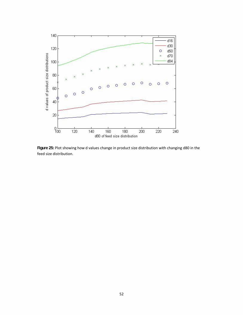
52

Figure 25: Plot showing how d values change in product size distribution with changing d80 in the feed size distribution.

53

Chapter 9: The effect of changing throughput of granite to gyratory crushers

The effect of changing the throughput into the gyratory crusher has also been quantified, and the effect that changing throughput has on both product size distribution and power draw. Using JKSimMet the throughput was varied from zero tonnes per hour up to 1000 tonnes per hour. It was found that the throughput has absolutely no effect on the product size distribution. This is consistent with previous findings using JKSimMet, showing that JKSimMet has no sensitivity at all to the feed throughput when giving product size distributions for a gyratory crusher. (Lowndes, 2007)

Through put (t/hr) Model Calculated Power (kW) Calculated Pendulum Power (kW)1 80.02 0.01885 80.12 0.0939

10 80.24 0.18825 80.61 0.4750 81.22 0.939

100 82.44 1.879200 84.89 3.758300 87.33 5.637400 89.77 7.516500 92.21 9.395600 94.66 11.27700 97.1 13.15800 99.54 15.03900 102 16.91

1000 104.4 18.79Table 7: Calculated power draw and the pendulum power of the gyratory crusher for different throughputs.

54

Figure 26: Power Draw Plotted against Throughput

Figure 27: Pendulum Power plotted against Throughput

55

A linear relationship was observed between the throughput and the power draw, and also between the throughput and the pendulum power (Table 7). The pendulum power is the power that is required to crush to the resultant size distribution in laboratory tests. It is linearly related to the total power draw as shown in equation 19.

It was also noted that the power draw for zero throughput is still quite high (figures 26 and 27). It is exactly the same number as the power draw approached asymptotically when plotting gap size against power draw as the gap size became large enough for all the feed to fall straight through. This is the minimum power draw of the crusher and it shows a considerable amount of the energy used to operate the crusher is not used for the crushing of the rock at all. This is confirmed from observations from site.

56

Chapter 10: Effect of changing ore type on JKSimMet performance

An investigation was conducted as to whether JKSimMet was sensitive to the ore type that was being crushed in the gyratory and cone crushers. This was carried out using the drop weight testing data from Ruszala’s MRes Thesis (appendix 3). This data could be entered directly into JKSimMet, the data that was entered was the appearance functions. Then keeping all the parameters of the crusher constant, the effect of changing the ore type on the product size distribution and also on the power draw could be investigated. The results were somewhat surprising in that it seemed the ore type had very little effect on the product size distribution (figure 28) or on the power draw of the crusher(table 8), (figure 29). It was expected that harder rocks would require more energy to crush effectively. There are a number of reasons why this may have been the case. It may be that JKSimMet is not as sensitive to ore type as it should be, or it may be that this is also the case in real crushing processes. The feed size distribution into the gyratory crusher is directly from the blasting phase and therefore a large proportion of the feed consists of very coarse rock particles. These are large enough to have cracks and structural weaknesses, so the crushing action would cause fracture at these points and the rock hardness would have very little effect on the power draw because of this. The paper on the impact of rock hardness by Kujundzic et al. (2008) also came to the conclusionthat the rock hardness had very little effect on the power draw of the crusher. The rock hardness has a greater effect in the blasting phase and the milling stages (when utilised) than it does in the primary crushing phase. It could be suggested that it is highly unrealistic when trying to model the whole Mine-to-Mill process to use the same feed size distribution for the primary crusher. It wouldbe more realistic to try and use a fragmentation model such as the Kuz-Ram distribution or the JK model with constant blast conditions to generate the different feed size distributions for each ore type. This could then be entered into JKSimMet to see what effect the rock type has on the product size distribution of the primary crusher with the blasting phase having been taken into account.

57

Rock Type Calculated Power Calculated Pendulum Power d50BIF Ore 102.1 16.99 50.92021Copper Carbonatite 103.2 17.83 51.7859Hard Talc 103.4 18.01 52.76697Lead-zinc Ore 102.8 17.52 50.93298Limestone 103 17.72 51.37417Poryphory Copper 102.6 17.38 51.10525Basalt 103.2 17.85 51.55975Granite 103 17.71 51.79715Table 8: Data from JKSimMet for different ore types passing through gyratory crusher

Figure 28: Product size distributions for different rock types from Gyratory crusher under similar operating conditions

Particle size (mm)

Cum

ulat

ive

perc

enta

ge p

assi

ng

58

Figure 29: Power Draw of gyratory crusher compared to d50 value for each ore type.

The Kuz-Ram distribution is known to underestimate the proportion of fine particles produced when blasting occurs.

There are a large number of parameters that are included in the Kuz-Ram model. The characteristics of the rock that is being blasted is noted as being important, with density, Youngs Modulus and rock hardness all being taken into account. There is also a term for the explosives that is included in the model, the mass of the explosive and the relative weight strength of the explosive used compared to ANFO. The blast hole design is also important, with terms for burden, spacing, bench height, hole diameter all included.

The only thing that will be changed in the Kuz-Ram distribution for different ore types therefore will be the characteristics of the rock. The blast design and the explosive parameters will be kept constant. It is expected that the Kuz-Ram model will generate very similar size distributions for rock types of similar hardness, as there will be hardly any changes in most parameters of the model. The only term that will be changing is A, at the front of the Kuznetsov equation.

The Kuz-Ram model has been entered into Matlab (Appendix 1). The parameters that have been entered have been found in various papers. The parameters that are used are shown in table 9. And the equations are written out below.

59

Parameter Value usedQ (size of blast hole charge (kg)) 224Sanfo (weighted strength of explosive) 80q (specific charge of explosive) 0.5RMD (rock mass description) 10RDI (rock density influence (kg/m3)) 0.025*ρ - 50ρ (density (kg/m3)) 3200HF (rock hardness factor) 30B (burden (m)) 4.5S (spacing (m)) 4.25φ (hole diameter (m)) 0.115Lb (length of bottom charge in blast hole (m)) 3Lc (length of column charge (m)) 6Ltot (total charge length (m)) Lb + LcH (bench height (m)) 19SD (standard deviation of drilling accuracy) 0.1Table 9: Parameters used to find Kuz-Ram distribution

X50 = AQ1/6(115/Sanfo)19/30q-4/5 (21)

A = 0.06(RMD + RDI + HF) (22)

P = 1 – exp(-log(2)(x/x50)n) (23)

N = (2.2 – 0.014B/φ)(1-SD/B)1/2(0.5(1+S/B))(abs((Lb-Lc)/Ltot)+0.1)0.1(Ltot/H) (24)

Equation 21 is the Kuznetsov equation for the value of x50, the mean particle size produced in the blast. Equation 22 gives the constant A to be used in the Kuznetsov equation and is the sum of the rock mass description, the rock density index and the rock hardness factor. Equation 23 is the Rosin Rammler distribution; it uses x50 as calculated by the Kuznetsov equation and calculates the percentage of rock passing each size value x. Equation 24 gives the value of n, the exponent in the Rosin-Rammler equation. This equation is in terms of the blast design parameters. A similar set of equations are given by Csoke et al. (1996). It is important to note that these equations for the Kuz-Ram distribution differ from paper to paper and have been modified many times as they are based on empirical observations from blasting experiments, and the results from different experiments will inevitably differ.

60

Figure 30: Kuzram Distribution generated in Matlab

Figure 30 shows a typical Kuz-ram distribution. This has been generated using the parameters shown in table 9. These values were based on the values given by Kanchibotla et al. There is a problem with just using the size distribution generated by the Kuz-ram distribution and putting it straight into JKSimMet to calculate the product size distribution. In reality when rock is blasted there will be some particles in the muckpile that are too coarse to fit into the crusher, these have to be crushed separately so that they fit into the crusher. The Kuz-ram distribution does not reach 100% until the sizes are much larger than the maximum size that can be fed into a gyratory crusher or entered in as a feed size distribution on JKSimMet. Therefore the size distributions that have been generated in this way have had to be skewed slightly

The equations in Matlab generate a cumulative size distribution, and interpolation is used to generate the cumulative percentage passing each size bracket on the list below which can be entered into JKSimMet. It is difficult to change the parameters of the Kuznetsov equation for each rock type. Parameters like rock hardness factor and the rock mass description are not necessarily exact properties that can be measured; only a sensible estimate can be made. As some of the ores looked at previously have similar properties it is therefore very difficult to put in parameters that represent each ore in the Kuznetsov equation. Therefore the parameters have been altered to alter the overall value of the constant A by different amounts, and then the value of d50 from the resulting distributions can be calculated and plotted against the value of A. This will at least show how the size distribution will alter with changing the characteristics of the feed rock. There are still problems with this approach however, as when blast designers are engineering a blast the properties of the rock will obviously alter the other parameters of the blast. So different blast design

61

parameters and explosive parameters will be used for different rock types, whereas in this case all these parameters have been kept constant which is clearly unrealistic. It is still a useful exercise however to see just what effect the rock hardness has on the size distribution with all the other conditions kept the same according to the Kuz-Ram distribution.

Figure 31: d50 of product size distribution varying with parameter A in Kuznetsov equation.

It has been seen that there is a relationship between the value of A in the Kuznetsov equation and the value of d50 for the product size distribution of the gyratory crusher (figure 31). This is as expected as the Kuznetsov equation was clearly sensitive to the parameters describing the physical properties of the rock, and it is already known that there is a relationship between the feed size distribution and the product size distribution of the gyratory crusher. This has therefore shown that even though in the primary crushing stages there is very little sensitivity to the rock type, it is still clearly an important factor to take into account because of the effect that it has in the blasting phase.

62

Chapter 11: Conclusion

The properties of granite have been reviewed and used to consider the mine to mill process at Mountsorrel Granite Quarry in Leicestershire. The microstructure of granite was considered and it was found from the literature that mechanical strength of granite decreases with increasing grain size as the rock tends to fracture along grain boundaries. It was also found that mechanical strength tended to decrease with increasing porosity. Different methods for measuring the physical properties of granite and also the microstructure have been considered including X-ray fluorescence, X-ray diffraction for measuring the elemental composition and also drop weight testing for measuring the mechanical strength. It was found that data found from drop weight testing could be used in the modelling of crushing processes. Drop weight testing provided information for the breakage matrix that could be entered into JKSimMet so that the way different ore types are crushed in a gyratory crusher could be simulated.

Comminution processes at the Mountsorrel Granite Quarry in Leicestershire have been considered. The blasting process has been reviewed as has the primary and secondary crushing stages. The blast design was shown to be very important not only in minimising fines produced in that phase, but also having an effect on downstream operations. It showed that the processes needed to be optimised individually and that the whole mine to mill process needed to be considered as well. Various size distributions were considered from the literature that attempted to model the blasting process.

At Mountsorrel quarry a gyratory crusher is used for the primary crushing stage and a cone crusher is used for the secondary crushing. These can be simulated using JKSimMet, a flowsheet representing the crushing and screening processes that take place at Mountsorrel Quarry has been drawn and is used to simulate the individual processes at the quarry.

Changing the gap size on both the gyratory crusher and the cone crusher were investigated and the effects that this had on the product size distribution and also on the energy imput by the crusher. All other factors were kept constant. Using the curve fitting software Gnuplot it was found that there is a functional relationship between the CSS and the product size distribution for both the gyratory and the cone crusher. This relationship was found to be of the same form as the Rosin-Rammler distribution.

Changing the feed size distribution for the gyratory crusher was also investigated using JKSimMet. It was found that there was a relationship between the feed size distribution and the product size distribution, but that the relationship did not fit to a function easily like the relationship between the CSS and the product size distribution. There was no real relationship between the feed size distribution and the energy input.

Changing the throughput was also investigated; this had no effect whatsoever on the product size distribution as expected. There was a linear effect on the power draw and on the pendulum power draw. It was noted that the power draw when the throughput was zero was exactly the same as the value that the power draw asymptoted to as the CSS increased.

Finally the effect of ore type on the product size distribution and power draw was investigated. It was found that changing the ore type had virtually no effect on the product size distribution on

63

JKSimMet, this was found to be consistent with experimental investigations in the literature. It was also found that there was no discernible effect between the ore type and the power draw of the crusher.

To investigate the effect that ore type has on the whole mine to mill process the effect on the blasting phase was investigated. To do this the Kuz-Ram equation was used. This generated a size distribution for each ore type simulating the blasting of these ores. The other parameters in the Kuznetsov equation were kept constant. It was found in this way that the ore type does have an effect on the blasting phase, and since changing the feed size distribution affects the product size distribution of the crushers, changing the ore type will affect the overall mine to mill process, and must be taken into account in the optimisation process.

11.2 Future Work

It remains to be seen whether these results will match up with experimental data. However it is expected that it will seeing as JKSimMet has already been shown to be a good simulator for comminution processes, notwithstanding the issues with rock throughput and ore type.

The next phase is to try and combine the functional relationships that have so far been found into one easy to use software package that will simulate the whole process at Mountsorrel quarry.

64

References

Andersen, J.S., Napier-Munn, T.J., (1990). The Influence of Liner Condition on Cone Crusher Performance. Minerals Engineering 3(1): 105-116

Bearman, R.A., Briggs, C.A., Kokovic, T., (1997). The Application of Rock Mechanics Parameters to the Prediction of Comminution Behaviour. Minerals Engineering 10(3): 255-264

Bilodeau, M., Labrie, D., Boisclair, M., Beaudoin, R., Roy, D., Caron, G., (2007). Impact of Electronic Blasting Detonators on Downstream Operations of a Quarry. SME Annual Meeting, 25-27 Feb 2007, Denver, Colorado.

Chaki, S., Takarli, M., Agbodjan, W.P., (2008). Influence of Thermal Damage on Physical Properties of a Granite Rock: Porosity, Permeability and Ultrasonic Wave Evaluations. Construction and Building Materials 22: 1456-1461

Chang, S. H., Chung-In, L., Seokwon, J., (2002). Measurement of Rock Fracture Toughness Under Modes I and II and Mixed-mode Conditions by Using Disc-type Specimens. Engineering Geology 60: 79-97

Csöke, B., Pethö, S., Földesi, J., Mészáros, L., (1996). Optimisation of Stone Quarry Technologies. International Journal of Mineral Processing 44-45: 447-459

David, C., Menendez, B., Darot, M., (1999). Influence of Stress-induced and Thermal Cracking on Physical Properties and Microstructure of La Peyrette Granite. International Journal of Rock Mechanics and Mining Sciences 36: 433-448

Donovan, J.G., (2003). Fracture Toughness Based Models for the Prediction of Power Consumption, Product Size, and Capacity of Jaw Crushers. Dissertation submitted to theFaculty of the Virginia Polytechnic Institute and State University.

Eberhardt, E., Stimpson, B., Stead, D., (1999). Effects of Grain Size on the Initiation and Propagation Thresholds of Stress-Induced Brittle Fractures. Rock Mechanics and Rock Engineering, 32(2), 81-99

El-Taher, A., (2012). Elemental Analysis of Granite by Instrumental Neutron Activation Analysis (INAA) and X-Ray Fluorescence. Applied Radiation and Isotopes 70: 350-354

Gheibie, S., Aghababaei, H., Hoseinie, S.H, Pourrahimian, Y., (2009). Modified Kuz-Ram Fragmentation Model and its Use at the Sungen Copper Mine. International Journal of Rock Mechanics and Mining Sciences 46: 967-973

Gongbo, L.I., Xiaohe, X.U., (1993). Experimental Investigation of the Energy Size Reduction Relationship in Comminution Using Fractal Theory. Minerals Engineering 6(2): 163-172

Guthrie, J.M., (2012). Overview of X-Ray Fluoresence. University of Missouri Research Reactor. http://archaeometry.missouri.edu/xrf_overview.html. (accessed 13/09/14)

Hosseinzadeh, H., Ergun, L., (2012). Determination of Breakage Distribution Function of Fine Chromite Ores with Bed Breakage Method. XIII International Mineral Processing Symposium

Hu, H., Xiaolin, S., Zhang, M., (2011). The Influence of Granite Microstructure on the Properties of Pavement Material. International Conference on Electric Technology and Civil Engineering: 6311-6314

Hudaverdi, T., Kuzu, C., Fisne, A., (2012). Investigation of the Blast Fragmentation Using the Mean Fragment Size and Fragmentation Index. International Journal of Rock Mechanics and Mining Sciences 56: 136-145

65

Inglis, C.E. (1913), Stresses in a Plate Due to the Presence of Cracks and Sharp Corners, Read at the Spring Meetings of the Fifty-fourth Session of the Institution of Naval Architects on March 14 1913

JKSimMet (2003). Steady State Mineral Processing Simulator. JKMRC. Kanchibotla, S.S., Morrel, S., Valery, W., O’Loughlin, P., (1998) Exploring the Effect of Blast

Design on SAG Mill Throughput at KCGM. Kojovic, T., Napier-Munn, T.J., Andersen, J.S., (1998).Modelling Cone and Impact Crushers

Using Laboratory Determined Energy Breakage Functions. Comminution Practices: Chapter 8 Kujundžic, T., Bedeković, G., Kuhinek, D., Korman, T., (2008). Impact of Rock Hardness on

Fragmentation by Hydraulic Hammer and Crushing in Jaw Crusher. Rudarsko-geološko-naftni zbornik 20: 83-90

Lafarge Aggregates Ltd (2006). A Guide to Mountsorrel Quarry. Available at: <http://www.lafarge.co.uk/pdf/A_Guide_to_Mountsorrel_Quarry.pdf> (accessed 13/09/14)

Lindqvist, J.E., Malaga, K., Middendorf, B., Savukosi, M., Petursson, P., (2007). Frost Resistance of Natural Stone, the Importance of Micro- and Nano-Porosity. Icelandic Building Research Institute

Lowndes, I., Jeffey, K., (2007). Optimising the Efficiency of Primary Aggregate Production. Available at: <http://www.sustainableaggregates.com/library/docs/mist/l0022_t2b_oepap.pdf>

Ludivico-Marques, M., Chastre, C., Vasconcelos, G., (2012). Modelling the Compressive Mechanical Behaviour of Granite and Sandstone Historical Building Stones. Construction and Building Materials 22: 372-381

Morin, M.A., Ficarazzo, F., (2006). Monte Carlo Simulation as a Tool to Predict Blasting Fragmentation Based on the Kuz-Ram Model. Computers and Geosciences 32(2): 352-359

http://www.niton.com/en/portable-xrf-technology/how-xrf-works/x-ray-fluorescence-(edxrf)-overview (accessed 13/09/14)

Roweis, S., (1996). Levenberg-Marquardt Optimisation. University of Toronto. Ruzsala, M.J.A., (2012). Fines Reduction and Energy Optimisation in Aggregates Reduction.

University of Birmingham. Sabih, A., Nemes, J.A., (2012). Experimental and finite element simulation study of the

adiabatic shear band phenomenon in cold heading process. Journal of Materials ProcessingTechnology 212: 1089-1105.

Tarmac Ltd and Partners, (2011). Towards meeting the challenges of sustainable aggregates production. Mine-to-Mill Process. Final Project Report. Available at: (accessed 13/09/14)http://www.sustainableaggregates.com/library/docs/mist/l0008_ma_7_g_5_004.pdf

Tavares, L.M., (1999). Energy Absorbed in Breakage of Single Particles in Drop Weight Testing. Minerals Engineering 12 (1): 43-50

Whiten, W.J., (1972). The Simulation of Crushing Plants with Models Developed Using Multiple Spline Regression. Journal of the South African Institute of Mining and Metallurgy:257-264

National Park Service Handbook for the Storage, Transportation, Training for Explosives Use, and Handling of Explosives, (1999). Chapter 8, Blast Design. 113-122. Available at: http://www.nps.gov/history/history/online_books/npsg/explosives/Chapter8.pdf (accessed 13/09/14)

66

Appendix 1 – Matlab Codes

A: Gap size of gyratory crusher, percentage passing 50 mm

clcclear all

load('gyratorycrushercssdata.txt'); %Loads the text file with all the data from changing the CSS value of the gyratory crusher.data = gyratorycrushercssdata;ng = length(data(1,:))/3;sdd{1,ng} = [];

for i = 1:ngsdd{1,i} = zeros(31,2); %Preallocated for speedend

for i = 1:ng sdd{1,i}(:,1) = data(1:31,3*i-2); %Size distribution cell array, every cell containing a size sdd{1,i}(:,2) = data(1:31,3*i); %distribution for a different gap size.end

for i = 1:ng

plot(sdd{1}(:,1),sdd{i}(:,2)) %Plot of these different size distributions hold onend

t50 = zeros(1,ng);css = 60:10:200;

for i = 1:ng t50(1,i) = interp1(sdd{i}(:,1),sdd{i}(:,2),50); %Calculates percentage passing 50mm for each size distribution end

figure(2) plot(css,t50) title('percentage of rock in product size distribution passing 50mm against CSS value of gyratory crusher') xlabel('CSS(mm)') ylabel ('% passing 50mm') cssi = 60:1:200; t50i = interp1(css,t50,cssi,'cubic'); %Interpolation used to estimate % what percentage passing 50mm for all gap sizes between 60 and 200mm would be interpolatedd50 = [cssi', t50i']; figure(3) plot(cssi,t50i) title('Interpolated Values of percentage of rock in PSD passing 50mm against CSS value of gyratory crusher')

xlabel('CSS(mm)')ylabel ('% passing 50mm')

67

B: Gap size of Gyratory Crusher, percentage passing 10 mm – 100 mm

clcclear all

load('gyratorycrushercssdatatonill.txt'); %Loads the text file with all the data from changing the CSS value of the gyratory crusher.data = gyratorycrushercssdatatonill;ng = length(data(1,:))/3;sdd{1,ng} = [];

for i = 1:ngsdd{1,i} = zeros(31,2); %Preallocates each cell of the array as a 31x2 matrix of zeroes.end

for i = 1:ng sdd{1,i}(:,1) = data(1:31,3*i-2); %Fills the first column of each ofthe cells with the size ranges sdd{1,i}(:,2) = data(1:31,3*i); %Fills the second column of each of the ceels with the percentage data. This is a size distribution for each value of CSS end %from 0 to 200mm.

for i = 1:ng

plot(sdd{1}(:,1),sdd{i}(:,2)) %Plots all the size distribution curves on the same graph title('Size distributions with different CSS values for each curve') xlabel('Size of rock(mm)') ylabel('cummulative percentage passing of rock that passes that size') hold on

endtx{1,9} = [];

for i = 1:9 tx{i} = zeros(1,ng); end

dy = [10,20,30,40,50,60,70,80,90]; %A vector created so that all the percentage values passing 10mm to 90mm can be calculated. css = 0:10:200;

for i = 1:9 for j = 1:ng tx{i}(1,j) = interp1(sdd{j}(:,1),sdd{j}(:,2),dy(i)); %Finds the values of t10 - t90 for each curve by interpolating over each size distribution. endend

figure(2)for i = 1:length(dy) plot(css,tx{i})hold on

68

title('d values of product size distribution against CSS value of gyratory crusher') xlabel('CSS(mm)') ylabel ('value of dx(mm)')end

txi{1,9} = [];cssi = 0:1:200;

for i = 1:9 txi{i} = interp1(css,tx{i},cssi,'cubic'); %Finds the value of tx for all %values of CSS in between the %ones already given by JKSimMet by interpolating over CSS.end interpolateddx{1,9} = []; for i = 1:9 interpolateddx{i} = [txi{i}',cssi']; %Fills each cell with a table of the data found %by interpolation. Each cell %represents t10 - t100 and in each cell %that value is given for all %the values of CSS that have %been interpolated over. end figure(3) for i = 1:9 plot(cssi,txi{i}) hold on title('Interpolated Values of percentage of rock in PSD passing each size value against CSS value of gyratory crusher') xlabel('CSS(mm)') ylabel ('percentage passing each size value') end

69

C: Functions for percentage passing size values with changing gap size found with GnuPlot

CSS = 50:200;

t90 = 1 + 95.9301*exp(log(0.2).*(CSS/9.62408).^-1.26562); %Uses function calculated by GnuPlot to calculatet80 = 1 + 90.9927*exp(log(0.2).*(CSS/20.414).^-1.57255); %percentage passing 90mm down to 10mm for each CSS valuet70 = 1 + 85.907*exp(log(0.2).*(CSS/31.3124).^-1.81438); %between 50 and 200mm.t60 = 1 + 81.3669*exp(log(0.2).*(CSS/40.7555).^-1.91719);t50 = 1 + 76.6362*exp(log(0.2).*(CSS/50.7655).^-2.03454);t40 = 1 + 73.4801*exp(log(0.2).*(CSS/57.7564).^-1.90378);t30 = 1 + 68.5709*exp(log(0.2).*(CSS/68.2918).^-1.99409);t20 = 1 + 64.3546*exp(log(0.2).*(CSS/74.7876).^-1.91117);t10 = 1 + 60.1796*exp(log(0.2).*(CSS/83.7717).^-1.87593);

plot(CSS,t10,'r',CSS,t20,'b',CSS,t30,'g',CSS,t40,'y',CSS,t50,'o',CSS,t60,'x',CSS,t70,'ro',CSS,t80,'go',CSS,t90,'yo')xlabel('CSS (mm)')ylabel('percentage of rocks passing each size (mm)')legend('10mm','20mm','30mm','40mm','50mm','60mm','70mm','80mm','90mm')

cssfunctiondatat10 = [CSS' t10'];cssfunctiondatat20 = [CSS' t20'];cssfunctiondatat30 = [CSS' t30'];cssfunctiondatat40 = [CSS' t40'];cssfunctiondatat50 = [CSS' t50'];cssfunctiondatat60 = [CSS' t60'];cssfunctiondatat70 = [CSS' t70'];cssfunctiondatat80 = [CSS' t80'];cssfunctiondatat90 = [CSS' t90'];

psdgn{1,length(CSS)} = [];for i = 1:length(CSS)psdgn{1,i} = zeros(9,2);

end

step = 10:10:90;

for i = 1:length(CSS) psdgn{1,i}(1,2) = t10(i); psdgn{1,i}(2,2) = t20(i); psdgn{1,i}(3,2) = t30(i); psdgn{1,i}(4,2) = t40(i); psdgn{1,i}(5,2) = t50(i); psdgn{1,i}(6,2) = t60(i); psdgn{1,i}(7,2) = t70(i); psdgn{1,i}(8,2) = t80(i); psdgn{1,i}(9,2) = t90(i);for j = 1:9 psdgn{1,i}(j,1) = step(j);endfigure(2)hold onplot(psdgn{1,i}(:,1),psdgn{1,i}(:,2));

70

hold offend

psd{1,length(CSS)} = [];

for i = 1:length(CSS) psd{1,i} = zeros(31,2);endload('gyratorycrushercssdatatonill.txt');data = gyratorycrushercssdatatonill;

size = data(1:31,1);

71

D: Power Draw against changing gap size for Gyratory Crusher

clcclear all

load('gappower.txt'); %Loads power draw data found on JKSimMet stored as a spreadsheet.

data = gappower;

plot(data(:,1),data(:,2))xlabel('Closed Side Setting(mm)') %plot power draw against gap sizeylabel('power draw(kW)')

figure(2)plot(data(:,1),data(:,3))xlabel('Closed Side Setting(mm)') %Plot pendulum powerylabel('pendulum power(kW)')

gapi = 20:1:200;datai = interp1(data(:,1),data(:,2),gapi);

figure(3)plot(gapi,datai)

72

E: Lognormal Distribution

d50 = 97.0528;d84 = 196.851;

sd = d84/d50;

x = 1:500;y = logncdf(x,log(d50),1);

figure(1)plot(x,100*y)xlabel('particle size(mm)')ylabel('% passing each size') %Plot of lognormal distribution

data = [x',y'];

z = [444.5 317.5 254.0 190.5 127.0 63.50 38.10 25.40 20.32 15.24 10.16 5.080 2.540 1.905 1.270 0.965 0.635 0.483 0.203 0.000]; %Size values for size distributionsdd = zeros(1,length(z));

for i=1:length(z)sdd(i) = 100*interp1(x,y,z(i),'cubic');end

psd = [z',sdd']; %Product size distribution generated by log normal distribution

73

F: Rosin-Rammler Distribution

x = 1:444.5;

y = 1 - exp(log(0.2).*(x/180).^1.2); %The Rossin Rammler distribution is closer to what is used on JKSimMet than the Log normal distribution. This is the %cumulative Rossin Rammler distribtuion

plot(x,100*y);xlabel('particle size(mm)')ylabel('% passing each size')

data = [x' y'];

z = [444.5 317.5 254.0 190.5 127.0 63.50 38.10 25.40 20.32 15.24 10.16 5.080 2.540 1.905 1.270 0.965 0.635 0.483 0.203 0.000];sdd = zeros(1,length(z));

for i=1:length(z)sdd(i) = 100*interp1(x,y,z(i),'cubic');end

psd = [z',sdd'];

74

G: Changing Feed Size Distribution with Product Size Distribution

x = 1:444.5;

y = 1 - exp(log(0.2).*(x/180).^1.2); %The Rossin Rammler distribution is closer to what is used on JKSimMet than the Log normal distribution. This is the %cumulative Rossin Rammler distribtuion

plot(x,100*y);xlabel('particle size(mm)')ylabel('% passing each size')

data = [x' y'];

z = [444.5 317.5 254.0 190.5 127.0 63.50 38.10 25.40 20.32 15.24 10.16 5.080 2.540 1.905 1.270 0.965 0.635 0.483 0.203 0.000];sdd = zeros(1,length(z));

for i=1:length(z)sdd(i) = 100*interp1(x,y,z(i),'cubic');end

psd = [z',sdd'];

75

H: Changing Ore Type

clcclear all

load('differentores.txt'); %Loads data for different ore typessizedist = differentores;

ng = length(sizedist(1,:))/3;

for i = 1:ng hold on plot(sizedist(:,3*i-2),sizedist(:,3*i)) % Plots the size distributions for each ore on the same plotlegend('BIF ore','Copper carbonatite','Hard talc','Lead-zinc ore', 'Limestone', 'Porphory copper', 'Basalt', 'Granite')end

d50 = zeros(1,ng);

for i = 1:ng d50(1,i) = interp1(sizedist(:,3*i),sizedist(:,3*i-2),50);end

76

I: Power Draw for Changing Ore Type

clcclear all

load('powerdrawd50.txt');

data = powerdrawd50;

plot(data(:,1),data(:,3),'o');xlabel('d50 of product size distribution')ylabel('power draw (kW)')

77

J: Changing Throughput, pendulum power and power output

clcclear all

load('poweroutput.txt');data = poweroutput;

load('pendulumpower.txt');data2 = pendulumpower;

throughput = data(:,1);calcpower = data(:,2);pendpower = data2(:,2);

plot(throughput,calcpower)xlabel('throughput(t/hr)')ylabel('power draw(kW)')

figure (2)plot(throughput,pendpower)xlabel('throughput(t/hr)')ylabel('pendulum power(kW)')

78

K: Kuz-Ram Distribution

clear allclc

Q = 224; %size of blast hole charge(kg)sanfo = 80; %weight strength of explosive usedq = 0.5; % specific chargeRMD = 10; %rock mass description = JF if vertical jointsJF = 10; %joint factor = JPS + JPA JPS = 50; %joint plate spacingJPA = 50; %joint plate anglerho = 3200;RDI = 0.025*rho - 50; %rock density influenceHF = 30; %hardness factorB = 4.5; %burdenS = 4.25; %spacingphi = 0.115; %hole diameterLb = 3; %length of bottom chargeLc = 6; %length of column chargeLtot = Lb + Lc;H = 19; %bench heightSD = 0.1; %standard deviation of drilling accuracy

n = (2.2-0.014*B/phi)*(1-SD/B).^(1/2)*(0.5*(1+S/B))*(abs(Lb-Lc)/(Ltot) + 0.1).^(0.1)*(Ltot/H); %equation for finding exponent in Rosin-Rammler distribution%in terms of blast design parameters

A = 0.06*(RMD + RDI + HF); %equation for constant in Kuz equation taking rock properties into account

x50 = A*Q^(1/6)*(115/sanfo)^(19/30)*1/(q^(0.8)); %kuznetsov equation

x = zeros(1,1100);

for i = 1:100x(i) = i/100;

end

for i = 101:1100 x(i) = i - 99; %generates size vector so more values given at below 1mm where the percentage rise is steeperend

P = zeros(1,1100);

for i = 1:length(x) P(i) = 1 - exp(-log(2)*(x(i)/x50)^(n)); %Rosin Rammler distribution, using x50 from Kuz equation and exponent n from above equationend

plot(log(x),100*P)title('Kuzram Blast Model Size Distribution')

79

xlabel('log of particle size')ylabel('% passing')

xi = [444.5,317.5,254,190.5,127,63.5,38.1,25.4,20.32,15.24,10.16,5.080,2.540,1.905,1.270,0.965,0.635,0.483,0.203];

Pi = zeros(length(xi),1);for i = 1:length(xi) Pi(i,1) = 100*interp1(x,P,xi(i)); %Using interpolation to get percentage passing size values given in xi.end

figure(2)plot(xi,Pi)

80

L: Changing Size Distribution using Kuz Ram

clear allclc

load('kuzram.txt');

size = kuzram;ng = length(size(1,:))/3;

for i = 1:ng d50(i) = interp1(size(:,3*i),size(:,3*i-2),50); %finds d50 for each size distributionend

A = [3.375,3.975,4.2,4.575,4.8,5.175,5.4,5.775,6,6.6,7.775,8.175,8.4,8.775,9,9.375,9.6,9.975,10.2,10.8]; %different values of A that have been used in Kuzram distribution

plot(A,d50) %plots A against d50 of product size distribution of gyratory crusherxlabel('A, constant describing rock characteristics')ylabel('d50 (mm), mean rock size in product size distribution')

81

Appendix 2: JKSimMet Flowsheets

Feed Gyratory crusher Screen

Cone crusher Stock pile Splitter

82

Complete JKSimMet Flowsheet for Mountsorrel Quarry

83

Appendix 3: Appearance functions for different ore types found by drop weight testing

BIF Ore

Value of t10 t75 t50 t25 t4 t2

10 2.6 3.4 5.2 21.4 51.4 20 5.4 7.0 10.7 43.4 82.1 30 8.7 11.0 16.5 63.8 97.2

Copper Carbonatite

Hard talc

Value of t10 t75 t50 t25 t4 t2

10 3.2 3.9 5.5 23.9 53.2 20 6.5 7.9 11.2 44.8 84.5 30 10.0 12.1 17.0 62.6 99.1

Lead zinc ore

Value of t10 t75 t50 t25 t4 t2

10 2.7 3.3 5.0 23.3 52.7 20 5.7 6.9 10.3 43.3 81.7 30 9.0 10.8 15.9 60.1 94.2

Limestone

Value of t10 t75 t50 t25 t4 t2

10 2.4 3.0 4.9 23.7 59.8 20 4.7 6.0 9.6 45.0 87.9 30 7.2 9.2 14.7 62.8 96.4

Value of t10 t75 t50 t25 t4 t2

10 3.0 3.6 5.4 19.9 50.0 20 5.8 7.3 11.0 39.6 82.0 30 8.8 11.2 16.8 57.5 98.4

84

Value of t10 t75 t50 t25 t4 t2

10 3.1 3.7 5.4 23.3 55.4 20 6.5 7.8 11.2 44.4 85.1 30 10.1 12.2 17.3 62.5 96.9

Poryphory copper

Value of t10 t75 t50 t25 t4 t2

10 2.8 4 5.5 22.2 51.420 5.6 7.2 10.7 43.4 80.830 8.9 11.3 16.4 60.7 93

Basalt

Reference: (Ruszala, 2012)

85

Appendix 4: Size Distributions for Gyratory Crusher with Changing Gap Size

CSS = 60 mm

Size (mm)

Exp Sim

Top Size 200 0 0

Size 1 141.4 100 0.00104

Size 2 100 100 1.243

Size 3 70.71 100 9.317

Size 4 50 100 25.39

Size 5 35.36 100 44.92

Size 6 25 100 61.24

Size 7 17.68 100 72.23

Size 8 12.5 100 79.47

Size 9 8.839 100 84.4

Size 10 6.25 100 87.92

Size 11 4.419 100 90.53

Size 12 3.125 100 92.52

Size 13 2.21 100 94.07

Size 14 1.563 100 95.28

Size 15 1.105 100 96.24

Size 16 0.781 100 97

Size 17 0.552 100 97.6

Size 18 0.391 100 98.08

Size 19 0.276 100 98.46

Size 20 0.195 100 98.76

Size 21 0.138 100 99

Size 22 0.0977 100 99.19

Size 23 0.0691 100 99.35

Size 24 0.0488 100 99.48

Size 25 0.0345 100 99.58

86

Size 26 0.0244 100 99.66

Size 27 0.0173 100 99.73

Size 28 0.0122 100 99.78

Size 29 0.00863 100 99.82

Size 30 0 100 100

87

CSS = 70 mm

Size (mm) Exp Sim

Top Size 200 0 0

Size 1 141.4 100 0.0246

Size 2 100 100 3.462

Size 3 70.71 100 15.22

Size 4 50 100 33.94

Size 5 35.36 100 52.84

Size 6 25 100 66.81

Size 7 17.68 100 76.06

Size 8 12.5 100 82.21

Size 9 8.839 100 86.46

Size 10 6.25 100 89.52

Size 11 4.419 100 91.8

Size 12 3.125 100 93.54

Size 13 2.21 100 94.89

Size 14 1.563 100 95.95

Size 15 1.105 100 96.79

Size 16 0.781 100 97.45

Size 17 0.552 100 97.97

Size 18 0.391 100 98.38

Size 19 0.276 100 98.7

Size 20 0.195 100 98.96

Size 21 0.138 100 99.17

Size 22 0.0977 100 99.34

Size 23 0.0691 100 99.47

Size 24 0.0488 100 99.58

88

Size 25 0.0345 100 99.67

Size 26 0.0244 100 99.74

Size 27 0.0173 100 99.79

Size 28 0.0122 100 99.83

Size 29 0.00863 100 99.87

Size 30 0 100 100

89

CSS = 80 mm

Size (mm)

Exp Sim

Top Size 200 0 0

Size 1 141.4 100 0.539

Size 2 100 100 6.436

Size 3 70.71 100 21.29

Size 4 50 100 41.22

Size 5 35.36 100 58.77

Size 6 25 100 70.92

Size 7 17.68 100 78.92

Size 8 12.5 100 84.3

Size 9 8.839 100 88.04

Size 10 6.25 100 90.76

Size 11 4.419 100 92.79

Size 12 3.125 100 94.34

Size 13 2.21 100 95.54

Size 14 1.563 100 96.47

Size 15 1.105 100 97.21

Size 16 0.781 100 97.79

Size 17 0.552 100 98.24

Size 18 0.391 100 98.6

Size 19 0.276 100 98.88

Size 20 0.195 100 99.1

Size 21 0.138 100 99.28

Size 22 0.0977 100 99.42

Size 23 0.0691 100 99.53

Size 24 0.0488 100 99.62

Size 25 0.0345 100 99.69

Size 26 0.0244 100 99.75

90

Size 27 0.0173 100 99.8

Size 28 0.0122 100 99.84

Size 29 0.00863 100 99.87

Size 30 0 100 100

91

CSS = 90 mm

Size (mm)

Exp Sim

Top Size 200 0 0

Size 1 141.4 100 1.448

Size 2 100 100 9.796

Size 3 70.71 100 27.13

Size 4 50 100 47.27

Size 5 35.36 100 63.21

Size 6 25 100 73.96

Size 7 17.68 100 81.07

Size 8 12.5 100 85.89

Size 9 8.839 100 89.27

Size 10 6.25 100 91.73

Size 11 4.419 100 93.57

Size 12 3.125 100 94.97

Size 13 2.21 100 96.05

Size 14 1.563 100 96.89

Size 15 1.105 100 97.55

Size 16 0.781 100 98.06

Size 17 0.552 100 98.46

Size 18 0.391 100 98.78

Size 19 0.276 100 99.03

Size 20 0.195 100 99.23

Size 21 0.138 100 99.39

Size 22 0.0977 100 99.51

Size 23 0.0691 100 99.61

Size 24 0.0488 100 99.69

Size 25 0.0345 100 99.75

Size 26 0.0244 100 99.8

92

Size 27 0.0173 100 99.84

Size 28 0.0122 100 99.87

Size 29 0.00863 100 99.9

Size 30 0 100 100

93

CSS = 100 mm

Size (mm) Exp Sim

Top Size 200 0 0Size 1 141.4 100 2.718Size 2 100 100 13.32Size 3 70.71 100 32.44Size 4 50 100 52.17Size 5 35.36 100 66.63Size 6 25 100 76.3Size 7 17.68 100 82.74Size 8 12.5 100 87.13Size 9 8.839 100 90.23Size 10 6.25 100 92.49Size 11 4.419 100 94.18Size 12 3.125 100 95.47Size 13 2.21 100 96.46Size 14 1.563 100 97.22Size 15 1.105 100 97.81Size 16 0.781 100 98.27Size 17 0.552 100 98.63Size 18 0.391 100 98.91Size 19 0.276 100 99.13Size 20 0.195 100 99.3Size 21 0.138 100 99.44Size 22 0.0977 100 99.55Size 23 0.0691 100 99.64Size 24 0.0488 100 99.71Size 25 0.0345 100 99.77Size 26 0.0244 100 99.81Size 27 0.0173 100 99.85Size 28 0.0122 100 99.88Size 29 0.00863 100 99.9Size 30 0 100 100

94

CSS = 110 mm

Size (mm) Exp Sim

Top Size 200 0 0Size 1 141.4 100 4.246Size 2 100 100 16.85Size 3 70.71 100 37.08Size 4 50 100 56.08Size 5 35.36 100 69.35Size 6 25 100 78.19Size 7 17.68 100 84.11Size 8 12.5 100 88.17Size 9 8.839 100 91.04Size 10 6.25 100 93.14Size 11 4.419 100 94.71Size 12 3.125 100 95.9Size 13 2.21 100 96.81Size 14 1.563 100 97.5Size 15 1.105 100 98.04Size 16 0.781 100 98.46Size 17 0.552 100 98.79Size 18 0.391 100 99.04Size 19 0.276 100 99.24Size 20 0.195 100 99.4Size 21 0.138 100 99.52Size 22 0.0977 100 99.62Size 23 0.0691 100 99.7Size 24 0.0488 100 99.76Size 25 0.0345 100 99.81Size 26 0.0244 100 99.85Size 27 0.0173 100 99.88Size 28 0.0122 100 99.9Size 29 0.00863 100 99.92Size 30 0 100 100

95

CSS = 120 mm

Size (mm) Exp Sim

Top Size 200 0 0Size 1 141.4 100 6.044Size 2 100 100 20.41Size 3 70.71 100 41.05Size 4 50 100 58.95Size 5 35.36 100 71.25Size 6 25 100 79.51Size 7 17.68 100 85.15Size 8 12.5 100 89.09Size 9 8.839 100 91.81Size 10 6.25 100 93.75Size 11 4.419 100 95.19Size 12 3.125 100 96.29Size 13 2.21 100 97.16Size 14 1.563 100 97.83Size 15 1.105 100 98.35Size 16 0.781 100 98.74Size 17 0.552 100 99.04Size 18 0.391 100 99.27Size 19 0.276 100 99.44Size 20 0.195 100 99.57Size 21 0.138 100 99.67Size 22 0.0977 100 99.75Size 23 0.0691 100 99.81Size 24 0.0488 100 99.86Size 25 0.0345 100 99.89Size 26 0.0244 100 99.92Size 27 0.0173 100 99.94Size 28 0.0122 100 99.96Size 29 0.00863 100 99.97Size 30 0 100 100

96

CSS = 130 mm

Size (mm) Exp Sim

Top Size 200 0 0Size 1 141.4 100 7.668Size 2 100 100 23.53Size 3 70.71 100 44.52Size 4 50 100 61.63Size 5 35.36 100 73.14Size 6 25 100 80.85Size 7 17.68 100 86.06Size 8 12.5 100 89.66Size 9 8.839 100 92.22Size 10 6.25 100 94.09Size 11 4.419 100 95.48Size 12 3.125 100 96.52Size 13 2.21 100 97.31Size 14 1.563 100 97.91Size 15 1.105 100 98.37Size 16 0.781 100 98.73Size 17 0.552 100 99.01Size 18 0.391 100 99.22Size 19 0.276 100 99.38Size 20 0.195 100 99.51Size 21 0.138 100 99.61Size 22 0.0977 100 99.69Size 23 0.0691 100 99.75Size 24 0.0488 100 99.8Size 25 0.0345 100 99.84Size 26 0.0244 100 99.87Size 27 0.0173 100 99.89Size 28 0.0122 100 99.91Size 29 0.00863 100 99.93Size 30 0 100 100

97

CSS = 140 mm

Size (mm) Exp Sim

Top Size 200 0 0Size 1 141.4 100 9.444Size 2 100 100 26.5Size 3 70.71 100 47.4Size 4 50 100 63.64Size 5 35.36 100 74.51Size 6 25 100 81.82Size 7 17.68 100 86.78Size 8 12.5 100 90.22Size 9 8.839 100 92.66Size 10 6.25 100 94.44Size 11 4.419 100 95.76Size 12 3.125 100 96.75Size 13 2.21 100 97.5Size 14 1.563 100 98.06Size 15 1.105 100 98.49Size 16 0.781 100 98.82Size 17 0.552 100 99.08Size 18 0.391 100 99.28Size 19 0.276 100 99.43Size 20 0.195 100 99.55Size 21 0.138 100 99.64Size 22 0.0977 100 99.71Size 23 0.0691 100 99.77Size 24 0.0488 100 99.82Size 25 0.0345 100 99.86Size 26 0.0244 100 99.89Size 27 0.0173 100 99.91Size 28 0.0122 100 99.93Size 29 0.00863 100 99.94Size 30 0 100 100

98

CSS = 150 mm

Size (mm) Exp Sim

Top Size 200 0 0Size 1 141.4 100 11.21Size 2 100 100 29.15Size 3 70.71 100 49.8Size 4 50 100 65.31Size 5 35.36 100 75.66Size 6 25 100 82.65Size 7 17.68 100 87.41Size 8 12.5 100 90.71Size 9 8.839 100 93.05Size 10 6.25 100 94.76Size 11 4.419 100 96.02Size 12 3.125 100 96.96Size 13 2.21 100 97.67Size 14 1.563 100 98.2Size 15 1.105 100 98.61Size 16 0.781 100 98.92Size 17 0.552 100 99.16Size 18 0.391 100 99.34Size 19 0.276 100 99.48Size 20 0.195 100 99.59Size 21 0.138 100 99.68Size 22 0.0977 100 99.75Size 23 0.0691 100 99.8Size 24 0.0488 100 99.84Size 25 0.0345 100 99.87Size 26 0.0244 100 99.9Size 27 0.0173 100 99.92Size 28 0.0122 100 99.94Size 29 0.00863 100 99.95Size 30 0 100 100

99

CSS = 160 mm

Size (mm) Exp Sim

Top Size 200 0 0Size 1 141.4 100 12.93Size 2 100 100 31.51Size 3 70.71 100 51.78Size 4 50 100 66.67Size 5 35.36 100 76.59Size 6 25 100 83.31Size 7 17.68 100 87.9Size 8 12.5 100 91.09Size 9 8.839 100 93.35Size 10 6.25 100 95Size 11 4.419 100 96.22Size 12 3.125 100 97.12Size 13 2.21 100 97.79Size 14 1.563 100 98.29Size 15 1.105 100 98.68Size 16 0.781 100 98.97Size 17 0.552 100 99.2Size 18 0.391 100 99.37Size 19 0.276 100 99.5Size 20 0.195 100 99.6Size 21 0.138 100 99.68Size 22 0.0977 100 99.74Size 23 0.0691 100 99.79Size 24 0.0488 100 99.83Size 25 0.0345 100 99.86Size 26 0.0244 100 99.88Size 27 0.0173 100 99.9Size 28 0.0122 100 99.91Size 29 0.00863 100 99.92Size 30 0 100 100

100

CSS = 170 mm

Size (mm) Exp Sim

Top Size 200 0 0Size 1 141.4 100 14.59Size 2 100 100 33.6Size 3 70.71 100 53.42Size 4 50 100 67.8Size 5 35.36 100 77.38Size 6 25 100 83.89Size 7 17.68 100 88.34Size 8 12.5 100 91.44Size 9 8.839 100 93.64Size 10 6.25 100 95.24Size 11 4.419 100 96.41Size 12 3.125 100 97.28Size 13 2.21 100 97.93Size 14 1.563 100 98.41Size 15 1.105 100 98.78Size 16 0.781 100 99.06Size 17 0.552 100 99.27Size 18 0.391 100 99.43Size 19 0.276 100 99.55Size 20 0.195 100 99.65Size 21 0.138 100 99.72Size 22 0.0977 100 99.78Size 23 0.0691 100 99.83Size 24 0.0488 100 99.87Size 25 0.0345 100 99.9Size 26 0.0244 100 99.92Size 27 0.0173 100 99.94Size 28 0.0122 100 99.95Size 29 0.00863 100 99.96Size 30 0 100 100

101

CSS = 180 mm

Size (mm) Exp Sim

Top Size 200 0 0Size 1 141.4 100 16.17Size 2 100 100 35.44Size 3 70.71 100 54.75Size 4 50 100 68.7Size 5 35.36 100 78.01Size 6 25 100 84.35Size 7 17.68 100 88.7Size 8 12.5 100 91.72Size 9 8.839 100 93.86Size 10 6.25 100 95.41Size 11 4.419 100 96.55Size 12 3.125 100 97.39Size 13 2.21 100 98.01Size 14 1.563 100 98.47Size 15 1.105 100 98.82Size 16 0.781 100 99.09Size 17 0.552 100 99.29Size 18 0.391 100 99.45Size 19 0.276 100 99.57Size 20 0.195 100 99.66Size 21 0.138 100 99.73Size 22 0.0977 100 99.78Size 23 0.0691 100 99.82Size 24 0.0488 100 99.85Size 25 0.0345 100 99.88Size 26 0.0244 100 99.9Size 27 0.0173 100 99.92Size 28 0.0122 100 99.93Size 29 0.00863 100 99.94Size 30 0 100 100

102

CSS = 190 mm

Size (mm) Exp Sim

Top Size 200 0 0Size 1 141.4 100 17.64Size 2 100 100 37.04Size 3 70.71 100 55.87Size 4 50 100 69.45Size 5 35.36 100 78.54Size 6 25 100 84.75Size 7 17.68 100 89.01Size 8 12.5 100 91.97Size 9 8.839 100 94.06Size 10 6.25 100 95.58Size 11 4.419 100 96.69Size 12 3.125 100 97.51Size 13 2.21 100 98.12Size 14 1.563 100 98.57Size 15 1.105 100 98.91Size 16 0.781 100 99.17Size 17 0.552 100 99.37Size 18 0.391 100 99.52Size 19 0.276 100 99.63Size 20 0.195 100 99.72Size 21 0.138 100 99.79Size 22 0.0977 100 99.84Size 23 0.0691 100 99.88Size 24 0.0488 100 99.91Size 25 0.0345 100 99.93Size 26 0.0244 100 99.95Size 27 0.0173 100 99.97Size 28 0.0122 100 99.98Size 29 0.00863 100 99.99Size 30 0 100 100

103

CSS = 200 mm

Size (mm) Exp Sim

Top Size 200 0 0Size 1 141.4 100 18.99Size 2 100 100 38.43Size 3 70.71 100 56.84Size 4 50 100 70.11Size 5 35.36 100 79.01Size 6 25 100 85.1Size 7 17.68 100 89.28Size 8 12.5 100 92.18Size 9 8.839 100 94.23Size 10 6.25 100 95.72Size 11 4.419 100 96.8Size 12 3.125 100 97.59Size 13 2.21 100 98.18Size 14 1.563 100 98.61Size 15 1.105 100 98.94Size 16 0.781 100 99.19Size 17 0.552 100 99.38Size 18 0.391 100 99.52Size 19 0.276 100 99.63Size 20 0.195 100 99.71Size 21 0.138 100 99.77Size 22 0.0977 100 99.82Size 23 0.0691 100 99.86Size 24 0.0488 100 99.89Size 25 0.0345 100 99.91Size 26 0.0244 100 99.93Size 27 0.0173 100 99.94Size 28 0.0122 100 99.95Size 29 0.00863 100 99.96Size 30 0 100 100

104

Feed Size Distribution

Size (mm) Exp Sim

Top Size 444.5 100 100

Size 1 317.5 98.06 98.23

Size 2 254 92.52 92.78

Size 3 190.5 82.75 83.33

Size 4 127 65.24 70.79

Size 5 63.5 32.99 53.41

Size 6 38.1 19.39 28.98

Size 7 25.4 12.84 11.99

Size 8 20.32 10.28 5.9

Size 9 15.24 7.76 1.341

Size 10 10.16 5.27 0.516

Size 11 5.08 2.78 0.203

Size 12 2.54 1.5 0.0946

Size 13 1.905 1.17 0.042

Size 14 1.27 0.83 0.0204

Size 15 0.965 0.65 0.011

Size 16 0.635 0.46 0.00468

Size 17 0.483 0.36 0.0022

Size 18 0.203 0.18 0.00203

Size 19 0 0 0

Operating Data

Liner Length - LLen (mm) 50

Eccentric Throw - ET (mm) 10

Liner Hours - LHr (Hr) 0

Crusher Feed Rate (t/h) 500

Crusher Feed F80 (mm) 177.2

Crusher Product P80 (mm) 138.6

105

Appearance Function

Value of t10 t75 t50 t25 t4 t2

10 2.964 3.749 5.671 21.53 53.2

20 5.828 7.491 11.36 42.73 82.41

30 8.929 11.51 17.29 61.81 94.94