Modelling of a piled raft foundation as a plane strain...
118
Modelling of a piled raft foundation as a plane strain model in PLAXIS 2D A geotechnical case study of Nordstaden 8:27 Master of Science Thesis in the Master’s Programme Infrastructure and Environmental Engineering JOEL ALGULIN BJÖRN PEDERSEN Department of Civil and Environmental Engineering Division of GeoEngineering Geotechnical Engineering Research Group CHALMERS UNIVERSITY OF TECHNOLOGY Göteborg, Sweden 2014 Master’s Thesis 2014:131
Transcript of Modelling of a piled raft foundation as a plane strain...
Modelling of a piled raft foundation as a
plane strain model in PLAXIS 2D
A geotechnical case study of Nordstaden 8:27
Master of Science Thesis in the Master’s Programme Infrastructure and
Environmental Engineering
JOEL ALGULIN
BJÖRN PEDERSEN
Department of Civil and Environmental Engineering
Division of GeoEngineering
Geotechnical Engineering Research Group
CHALMERS UNIVERSITY OF TECHNOLOGY
Göteborg, Sweden 2014
Master’s Thesis 2014:131
joal
Ögonblicksbild

MASTER’S THESIS 2014:131
Modelling of a piled raft foundation as a
plane strain model in PLAXIS 2D
A geotechnical case study of Nordstaden 8:27
Master of Science Thesis in the Master’s Programme Infrastructure and
Environmental Engineering
JOEL ALGULIN
BJÖRN PEDERSEN
Department of Civil and Environmental Engineering
Division of GeoEngineering
Geotechnical Engineering Research Group
CHALMERS UNIVERSITY OF TECHNOLOGY
Göteborg, Sweden 2014

Modelling of a piled raft foundation as a plane strain model in PLAXIS 2D
A geotechnical case study of Nordstaden 8:27
Master of Science Thesis in the Master’s Programme Infrastructure and
Environmental Engineering
JOEL ALGULIN BJÖRN PEDERSEN
© JOEL ALGULIN & BJÖRN PEDERSEN, 2014
Examensarbete / Institutionen för bygg- och miljöteknik,
Chalmers tekniska högskola 2014:131
Department of Civil and Environmental Engineering
Division of GeoEngineering
Geotechnical Engineering Research Group
Chalmers University of Technology
SE-412 96 Göteborg
Sweden
Telephone: + 46 (0)31-772 1000
Cover:
Pore pressure distribution below cross-section K after ten years of consolidation and
an additional construction of two floors.
Chalmers Reproservice
Göteborg, Sweden 2014

I
Modelling of a piled raft foundation as a plane strain model in PLAXIS 2D
– A geotechnical case study of Nordstaden 8:27
Master of Science Thesis in the Master’s Programme Infrastructure and
Environmental Engineering
JOEL ALGULIN
BJÖRN PEDERSEN
Department of Civil and Environmental Engineering
Division of GeoEngineering
Geotechnical Engineering Research Group
Chalmers University of Technology
ABSTRACT
The aim of this report has been to, through a case study, investigate if a composite
foundation, consisting of a piled raft, is possible to model in a satisfying way with the
finite element computer software PLAXIS 2D, as well as investigate if an additional
construction of storeys would be possible on the existing foundation. For the case
study, a building in the shopping centre Nordstan in Gothenburg has been used.
Documentation in form of construction drawings, soil tests and reports regarding the
foundation of Nordstan has been used for the calculations. The soil model Soft Soil
has been used since it is suitable for modeling deformations of clay, like the one
present at the site of the case study. The structural element embedded pile row, which
provides the opportunity to set the out-of-plane distance in spite of the two-
dimensional modelling, has been used to model the piles. Different loading scenarios
have been used in order to predict settlements for addition of different number of
storeys. Comparisons between the soil models Soft Soil and Soft Soil Creep have
been performed as well as comparisons between rafts with and without piles. In the
conclusion it is stated that it seems possible to model the case study in a way that
gives reasonable results regarding settlements, which indicates that a two-dimensional
model can be a good and time efficient way to get a rough estimation of the capacity
of a piled raft foundation. The embedded pile row element has a reasonable behaviour
in the calculations, but comparisons to real testing of piles are needed. For further
studies new soil tests are also needed. The results indicate that construction of
additional storeys meets the demands regarding differential settlements and that
deformations at connections to surrounding streets more likely will set the limits of
design.
Key words: Piled raft, Plaxis 2D, Excavation, Settlements, Vertical soil
deformations, Soft Soil, Gothenburg, Nordstan, Östra Nordstaden,
Embedded pile row
II
Modellering av en samverkansgrundläggning som ”plane strain” model i PLAXIS 2D
– En geoteknisk fallstudie av Nordstaden 8:27
Examensarbete inom masterprogrammet Infrastructure and Environmental
Engineering
JOEL ALGULIN
BJÖRN PEDERSEN
Institutionen för bygg- och miljöteknik
Avdelningen för geologi och geoteknik
Forskargruppen för geoteknik
Chalmers tekniska högskola
SAMMANFATTNING
Denna rapports ändamål har varit att, genom en fallstudie, undersöka huruvida en
samverkansgrundläggning, bestående av en platta på pålar, går att modellera på ett bra
sätt i det finita element-datorprogrammet PLAXIS 2D samt om en eventuell
tillbyggnad av våningar skulle vara möjlig på den befintliga grundläggningen. Som
fallstudie har en byggnad i köpcentret Nordstan i Göteborg använts. Dokumentation i
form av konstruktionsritningar, jordtester samt rapporter om Nordstans grundläggning
har använts för beräkningar. Jordmodellen Soft Soil har använts eftersom den är
lämplig för att modellera sättningsbeteende i lerjordar likt den som finns vid
fallstudien. Konstruktionselementet ”embedded pile row”, vilket ger möjlighet att
ställa in avstånd i djupled trots tvådimensionell modellering, har använts för att
modellera pålarna. Olika lastscenarion har använts i beräkningar för att förutsäga
sättningar för olika antal våningar vid en eventuell tillbyggnad. Jämförelse mellan
jordmodellerna Soft Soil och Soft Soil Creep har utförts liksom en jämförelse mellan
plattor med och utan pålar. I rapportens slutsatser framkommer att fallstudien verkar
gå att modellera på ett sätt som ger rimliga resultat i form av sättningar, vilket
indikerar att en tvådimensionell modell kan vara ett bra och tidseffektivt sätt att få en
grov uppfattning av en samverkansgrundläggnings kapacitet. Pålelementet har ett
rimligt beteende i beräkningarna, men behöver jämföras med verkliga påltester. För
fortsatta studier behövs det även utföras nya jordtester. Resultat indikerar att eventuell
tillbyggnad klarar kraven för differentialsättningar och att sättningar vid förbindelser
med omkringliggande gator snarare kommer bli dimensionerande.
Nyckelord: Samverkansgrundläggning, Plaxis 2D, Schaktning, Sättningar, Vertikala
jorddeformationer, Soft Soil, Göteborg, Nordstan, Östra Nordstaden,
Embedded pile row
CHALMERS Civil and Environmental Engineering, Master’s Thesis 2014:131 III
Contents
ABSTRACT I
SAMMANFATTNING II
CONTENTS III
PREFACE VII
NOTATIONS VIII
1 INTRODUCTION 1
1.1 Background 1
1.2 Aim 1
1.3 Limitations 2
1.4 Methodology 2
2 BUILDING FOUNDATIONS ON SOFT COHESIVE SOIL 3
2.1 Raft foundation 3 Contact pressure and settlements 3 2.1.1
2.2 Compensated foundations 4
2.3 Piled foundations 5 Friction piles 6 2.3.1
Negative skin friction - Down drag 6 2.3.2
Neutral plane 6 2.3.3
Settlements for piled foundations 7 2.3.4
2.4 Composite foundation - Piled raft 9
The creep pile principle 10 2.4.1
2.5 Magnitude of allowable settlements for foundations on soft cohesive soil 11
3 CASE STUDY OF NORDSTADEN 8:27 12
3.1 History of the area 12
3.2 Geotechnical conditions 13
Geology 13 3.2.1
Hydrogeological conditions 14 3.2.2
Soil properties - parameter evaluation 14 3.2.3
3.3 Foundation of Nordstan 22
3.4 Principles behind the foundation method of building 6 26 Bearing capacity of the soil 27 3.4.1
Bearing capacity of the piles 28 3.4.2
Settlements readings 29 3.4.3
3.5 Loads acting on the foundation 29
4 NUMERICAL ANALYSES. MODELLING IN PLAXIS 2D 31
CHALMERS, Civil and Environmental Engineering, Master’s Thesis 2014:131 IV
4.1 Introduction to PLAXIS 2D 31
4.2 Soil models 32 Linear elastic (simplification of top layers) 32 4.2.1
Soft Soil (SS) 32 4.2.2
Soft Soil Creep (SSC) 33 4.2.3
4.3 Structural elements 35 Plate element 35 4.3.1
Embedded pile row element 36 4.3.2
4.4 Loads in PLAXIS 2D 39
5 VERIFICATION OF SOIL PARAMETERS AND SOIL MODELS 40
5.1 Soil tests performed in PLAXIS 2D 40
Axisymmetric model, Stepwise oedometer test 40 5.1.1
Triaxial soil test 41 5.1.2
5.2 Evaluating results 42 Stepwise oedometer simulations 42 5.2.1
Triaxial test simulations 46 5.2.2
6 MODELLING 47
6.1 Geometry and simplifications 47
6.2 Soil Model 50
6.3 Structural elements 51 Embedded pile row element 51 6.3.1
Plate element 52 6.3.2
6.4 Loads 53 Load scenarios 53 6.4.1
6.5 Mesh optimization 54
6.6 Phases 54
6.7 Validation analysis 55
6.8 Sensitivity analysis 55
7 RESULTS 57
7.1 Results from PLAXIS analyses 57 Excess pore water pressure 58 7.1.1
Settlements 60 7.1.2
Pile interaction 69 7.1.3
7.2 Sensitivity analyses results 71
7.3 Hand calculations 78 Stress distribution 78 7.3.1
Design demands 79 7.3.2
8 DISCUSSION 81

CHALMERS Civil and Environmental Engineering, Master’s Thesis 2014:131 V
9 CONCLUSIONS 83
10 REFERENCES 84

CHALMERS, Civil and Environmental Engineering, Master’s Thesis 2014:131 VI
CHALMERS Civil and Environmental Engineering, Master’s Thesis 2014:131 VII
Preface
This Master of Science Thesis has been conducted at the unit for geotechnical
engineering at ELU, Gothenburg, between January 7th
and June 18th
in 2014. The
project was initiated by ELU employees Bo Jansson and Lars Hall.
The authors would like to mention a number of people who have been of great help
and made this project possible:
We would like to thank our supervisor at ELU, Lars Hall, and ELU employee Therese
Hedman for support during the spring in 2014. Furthermore we would like to thank
the rest of the employees at ELU, especially Bo Jansson, Hans Lindewald, Mehras
Shahrestanakizadeh, Fredrik Olsson, Anders Beijer and Anna Iversen.
We would also like to thank Torbjörn Pettersson at Vasakronan, Malin Klarquist at
the Urban Planning Department of Gothenburg and Björn Petersson at WSP for
providing us with useful information about the building Nordstaden 8:27. Likewise
we would like to thank Professor Emeritus Sven Hansbo, responsible for the
foundation of the case study building, for explaining questions regarding his, at the
time unconventional, foundation method.
Lastly we would like to direct our appreciation to Professor Minna Karstunen at
Chalmers Univeristy of Technology for providing us with feedback as well as always
taking time to answer question and discuss different kinds problems encountered
during the process.
Gothenburg, June 2014
Joel Algulin and Björn Pedersen

CHALMERS, Civil and Environmental Engineering, Master’s Thesis 2014:131 VIII
Notations
Roman upper case letters
A cross section area of pile
B width of raft
vC
coefficient of consolidation
cC compression index
sC swelling index
C creep index
D depth of raft below closest adjacent surface
E Young’s modulus
ckE characteristic Young’s modulus for concrete
EA normal stiffness
1EA normal stiffness for plate element in PLAXIS 2D EI flexural rigidity
sG specific gravity
NCK
0 earth pressure coefficient for normally consolidated soil OC
K0 earth pressure coefficient for over consolidated soil
L length of raft
pL length of pile
pileiL length of pile part i in Figure 3.18
spacingL pile spacing perpendicular to the model plane
N bearing capacity of pile toe
O circumference of pile
OCR over consolidation ratio
R bearing capacity of pile
iR bearing capacity of pile part i in Figure 3.18
maxT skin resistance of embedded pile row element
max,topT skin resistance at pile top for embedded pile row element
max,botT skin resistance at pile bottom for embedded pile row element
CHALMERS Civil and Environmental Engineering, Master’s Thesis 2014:131 IX
Roman lower case letters
b width of plate element
'c cohesion for Mohr Coulomb criteria
uc corrected undrained shear strength
eqd equivalent thickness of plate element
id diameter at pile part i in Figure 3.18
piled diameter of pile
e void ratio
0e initial void ratio
h height of plate element
ph depth from +3.5 in Figure 3.18
k permeability
yk vertical permeability
xk horisontal permeability
vm coefficient of volume compressibility
'p mean effective stress '
pp effective preconsolidation pressure
POP over consolidation formulated as POP = '
c -
'
0
oilexcavatedsq weight of excavated soil
groundq bearing capacity of the ground
gnewbuildinq load from new building
pilesq bearing capacity of piles/area per pile
waterq uplifting water pressure
our dry density of timber
ur real density of timber
u moisture content
iu circumference at pile part i in Figure 3.18
pileu expression for circumference of lower pile part in Figure 3.18
platew weight of plate element material
Lw liquid limit
Nw natural water content
x length along raft from left to right
z depth from level y
CHALMERS, Civil and Environmental Engineering, Master’s Thesis 2014:131 X
Greek lower case letters
adhesion factor
rp ratio of load carried by piles for a piled raft
pile unit weight of pile material
soil unit weight of soil
w unit weight of pore water
one-dimensional strain
v0 initial volumetric strain
e
v0 initial volumetric strain during elastic response
v volumetric strain
c
v change of creep rate in time
e
v volumetric strain during elastic response
* modified swelling index
* modified compression index
* modified creep index
correction factor for undrained shear strength
Poisson’s ratio
concrete Poisson’s ratio of concrete
'
0 in-situ effective earth pressure
'
1 effective vertical earth pressure
'
3 effective horisontal earth pressure
'
c effective preconsolidation pressure
'
creep effective creep pressure
m bearing capacity of raft
reference time for oedometer test
fu undrained shear strength of the soil
' friction angle
dilatancy angle
CHALMERS, Civil and Environmental Engineering, Master’s Thesis 2014:131 1
1 Introduction
In 1970’s the shopping centre Nordstan was completed. Professor Sven Hansbo
implemented a new method when designing the foundation of the building. The
foundation method constitutes of a composite foundation with a piled raft, combined
with effects of uplifting water pressure and compensated weight of excavated soil.
Today, about 40 years later, the property owner, Vasakronan, is looking at the
possibility of expanding the building, by adding floors. To investigate if this is
possible, they have hired the consultancy company ELU.
This Master thesis was initiated with the belief that the foundation of Nordstan was
designed according to the creep pile principle. That kind of foundation method is
rather unusual today, which made ELU interested in the design and theory behind the
foundation method as well as whether or not it was possible to construct additional
floors.
1.1 Background
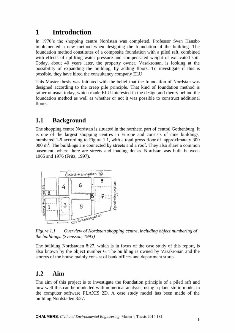
The shopping centre Nordstan is situated in the northern part of central Gothenburg. It
is one of the largest shopping centres in Europe and consists of nine buildings,
numbered 1-9 according to Figure 1.1, with a total gross floor of approximately 300
000 m2. The buildings are connected by streets and a roof. They also share a common
basement, where there are streets and loading docks. Nordstan was built between
1965 and 1976 (Fritz, 1997).
Figure 1.1 Overview of Nordstan shopping centre, including object numbering of
the buildings. (Svensson, 1993)
The building Nordstaden 8:27, which is in focus of the case study of this report, is
also known by the object number 6. The building is owned by Vasakronan and the
storeys of the house mainly consist of bank offices and department stores.
1.2 Aim
The aim of this project is to investigate the foundation principle of a piled raft and
how well this can be modelled with numerical analysis, using a plane strain model in
the computer software PLAXIS 2D. A case study model has been made of the
building Nordstaden 8:27.
CHALMERS, Civil and Environmental Engineering, Master’s Thesis 2014:131 2
The aim of the case study model in PLAXIS 2D, can be divided into the objectives
listed below:
Determine to what extent it is possible to model a piled raft, with the
complexity of Nordstan, as a plane strain problem in PLAXIS 2D.
Determine to what extent the structural element embedded pile row is working
when modelling a piled raft.
Determine what geotechnical effects increasing loads, due to additional
construction, would have in terms of settlements.
1.3 Limitations
When constructing on soft soil, deformations generally sets the limits for how large
loads can be applied to the foundation and is therefore the focus of this thesis.
The numerical calculations have been limited to 2D and only the building itself have
been taken into consideration for the numerical modelling. No consideration has been
taken to for example surrounding streets and buildings.
Construction drawings from before construction have been used as a basis for the
modelling and no consideration has been taken to any reconstruction. The property
owner states that the loads on acting on the foundation should be more or less the
same today as after reconstruction of the building1.
1.4 Methodology
In order to perform this investigation a literature survey regarding foundation
methods, commonly used on soft soil, have been carried out. Also a literature survey
of the foundation of the building, in the case study of Nordstaden 8:27, has been
carried out through articles, construction drawings, existing soil tests and
documentation of the building process. There was little documentation found
regarding the details of the design of building 6. However, such documentation was
found for building 5, which foundation was designed in a similar manner (Hansbo,
Hoffman and Mosesson, 1973).
Numerical analyses, with the finite element computer software PLAXIS 2D, have
been performed with focus on the real case scenario from Nordstan. The soil models
used in the case study model have been calibrated to match with existing soil tests. A
literature survey on different soil models and structural elements in PLAXIS has also
been made.
Elevation values mentioned in this thesis are corresponding to the local coordinate
system of Gothenburg used during the 20th century. In this system the datum line is
situated about 10 m below sea level.
1 Torbjörn Petterson, technical manager at Vasakronan, interviewed 14-02-20
CHALMERS, Civil and Environmental Engineering, Master’s Thesis 2014:131 3
2 Building foundations on soft cohesive soil
This chapter contains information about different foundation methods for constructing
buildings on clay.
The main purpose of a foundation is to transmit loads to the underlying soil. This
results in a soil-structure interaction. The foundation method which is most suitable
depends on the properties of the soil and the functional requirements of the building.
Since structural parts of a building often have higher stiffness and strength than
underlying soil, support is generally done by the use of shallow foundations (Hansbo,
1989). An example of this is enlarged ground plates (or slabs) which distributes the
loads over a larger area. However, if the soil stratum near the surface is not capable to
give sufficient support, deep foundations as piles or caissons may be used to transfer
the loads to larger depths, where the soil often has higher strength and stiffness (Craig
and Knappet, 2012).
2.1 Raft foundation
A large single slab which supports the structure as a whole is called a raft. Raft
foundations are used to distribute structural loads when the bearing capacity of the
underlying soil is low. A slab can cover the entire bottom area of the building or
several smaller ones can be strategically placed below pillars or walls (Hansbo, 1989).
A single raft is preferable in order to reduce differential settlements or when there are
local parts of the soil where the strength deviates. The raft can have an even thickness
or have stiffer parts where structural loads from walls or pillars are transmitted. It can
be designed with a stiffness large enough for the contact pressures to be assumed
equally distributed throughout the plate. Otherwise the distribution will depend on the
relative stiffness between plate and soil (Bergdahl, Malmborg and Ottosson, 1993).
Contact pressure and settlements 2.1.1
The distribution of the contact pressure depends on the mechanical properties of the
soil in combination with the stiffness of the foundation plate. The flexural rigidity of a
slab, resting on soil, is often very large compared to the deformability of the material
below (Hansbo, 1989).
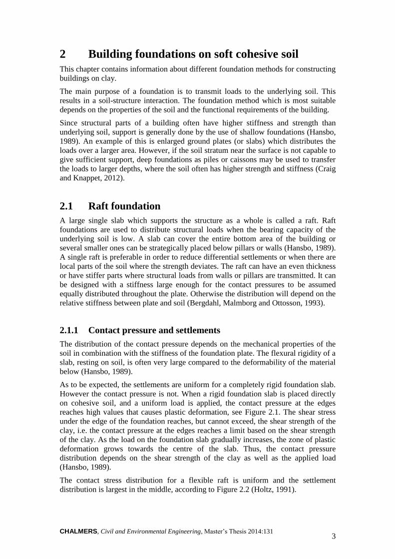
As to be expected, the settlements are uniform for a completely rigid foundation slab.
However the contact pressure is not. When a rigid foundation slab is placed directly
on cohesive soil, and a uniform load is applied, the contact pressure at the edges
reaches high values that causes plastic deformation, see Figure 2.1. The shear stress
under the edge of the foundation reaches, but cannot exceed, the shear strength of the
clay, i.e. the contact pressure at the edges reaches a limit based on the shear strength
of the clay. As the load on the foundation slab gradually increases, the zone of plastic
deformation grows towards the centre of the slab. Thus, the contact pressure
distribution depends on the shear strength of the clay as well as the applied load
(Hansbo, 1989).
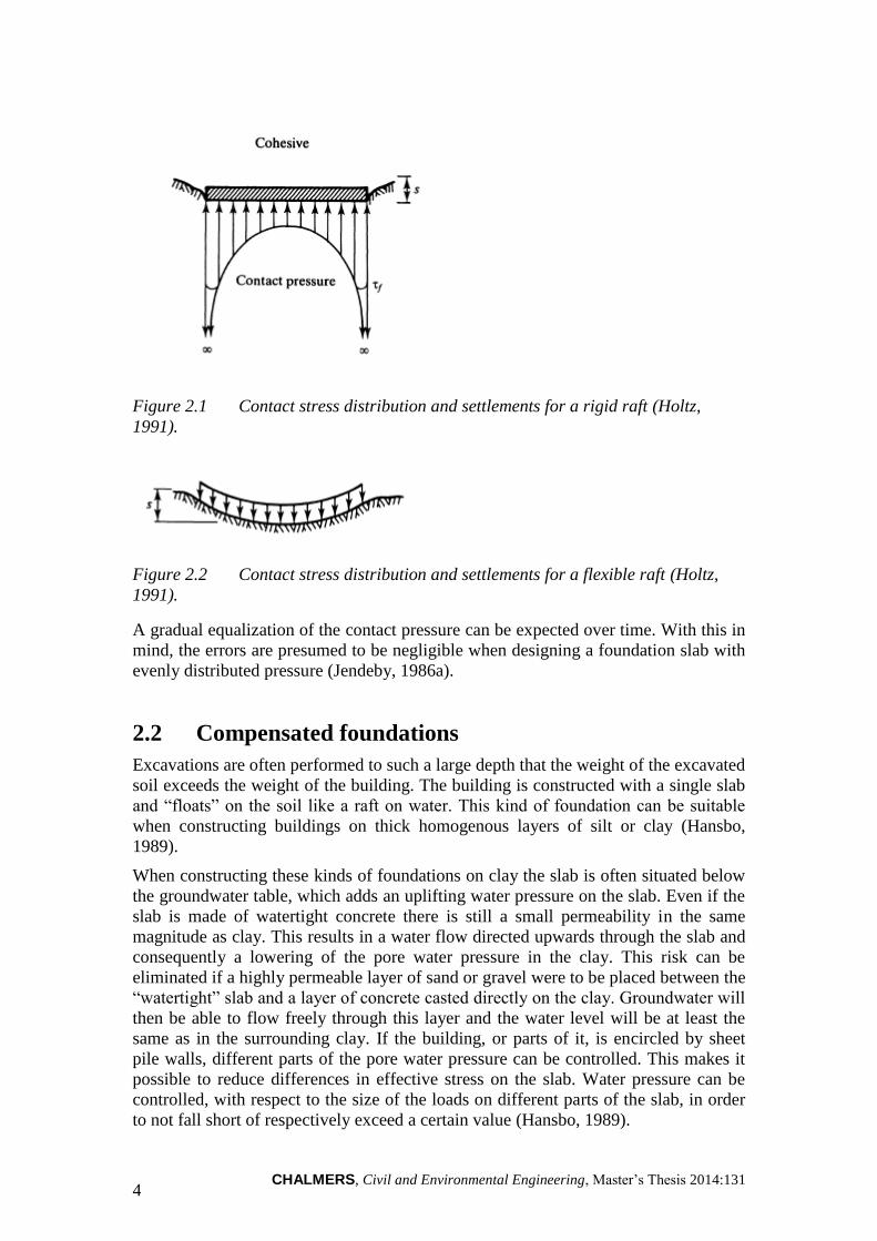
The contact stress distribution for a flexible raft is uniform and the settlement
distribution is largest in the middle, according to Figure 2.2 (Holtz, 1991).
CHALMERS, Civil and Environmental Engineering, Master’s Thesis 2014:131 4
Figure 2.1 Contact stress distribution and settlements for a rigid raft (Holtz,
1991).
Figure 2.2 Contact stress distribution and settlements for a flexible raft (Holtz,
1991).
A gradual equalization of the contact pressure can be expected over time. With this in
mind, the errors are presumed to be negligible when designing a foundation slab with
evenly distributed pressure (Jendeby, 1986a).
2.2 Compensated foundations
Excavations are often performed to such a large depth that the weight of the excavated
soil exceeds the weight of the building. The building is constructed with a single slab
and “floats” on the soil like a raft on water. This kind of foundation can be suitable
when constructing buildings on thick homogenous layers of silt or clay (Hansbo,
1989).
When constructing these kinds of foundations on clay the slab is often situated below
the groundwater table, which adds an uplifting water pressure on the slab. Even if the
slab is made of watertight concrete there is still a small permeability in the same
magnitude as clay. This results in a water flow directed upwards through the slab and
consequently a lowering of the pore water pressure in the clay. This risk can be
eliminated if a highly permeable layer of sand or gravel were to be placed between the
“watertight” slab and a layer of concrete casted directly on the clay. Groundwater will
then be able to flow freely through this layer and the water level will be at least the
same as in the surrounding clay. If the building, or parts of it, is encircled by sheet
pile walls, different parts of the pore water pressure can be controlled. This makes it
possible to reduce differences in effective stress on the slab. Water pressure can be
controlled, with respect to the size of the loads on different parts of the slab, in order
to not fall short of respectively exceed a certain value (Hansbo, 1989).
CHALMERS, Civil and Environmental Engineering, Master’s Thesis 2014:131 5
2.3 Piled foundations
When designing foundations with piles, the two main aspects to take into
consideration are bearing capacity and settlements. For a foundation on clay,
settlements are almost exclusively the limiting factor (Jendeby, 1986a).
The main reason for using piles in a foundation design is to transfer applied loads to a
greater depth of the soil. Deeper layers of the soil, due to their stress history, normally
have higher strength and stiffness compared to more shallow layers and therefore
would have greater resistance to settlement.
When a pile is subjected to a vertical force at the top of the pile, the pile head, shear
stresses are mobilised in the ground that surrounds the pile. If the created shear stress
exceeds the shear strength of the soil, ground failure will occur. Two different
parameters decide the capacity:
1. Shear stress that is developed in the soil around the pile toe
2. Shear stress that is developed at the interface between the shaft and the
surrounding soil.
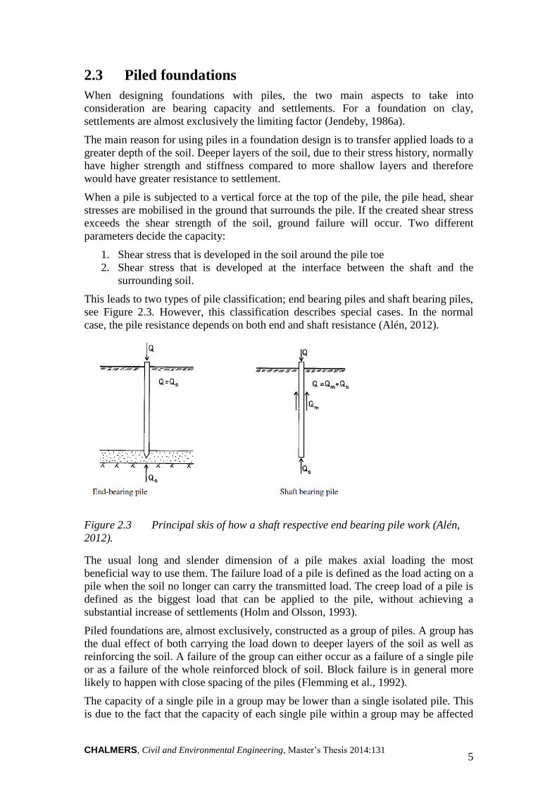
This leads to two types of pile classification; end bearing piles and shaft bearing piles,
see Figure 2.3. However, this classification describes special cases. In the normal
case, the pile resistance depends on both end and shaft resistance (Alén, 2012).
Figure 2.3 Principal skis of how a shaft respective end bearing pile work (Alén,
2012).
The usual long and slender dimension of a pile makes axial loading the most
beneficial way to use them. The failure load of a pile is defined as the load acting on a
pile when the soil no longer can carry the transmitted load. The creep load of a pile is
defined as the biggest load that can be applied to the pile, without achieving a
substantial increase of settlements (Holm and Olsson, 1993).
Piled foundations are, almost exclusively, constructed as a group of piles. A group has
the dual effect of both carrying the load down to deeper layers of the soil as well as
reinforcing the soil. A failure of the group can either occur as a failure of a single pile
or as a failure of the whole reinforced block of soil. Block failure is in general more
likely to happen with close spacing of the piles (Flemming et al., 1992).
The capacity of a single pile in a group may be lower than a single isolated pile. This
is due to the fact that the capacity of each single pile within a group may be affected
CHALMERS, Civil and Environmental Engineering, Master’s Thesis 2014:131 6
by the remoulding of surrounding soil, when other piles are installed in close
proximity (Flemming et al., 1992).
Friction piles 2.3.1
A friction pile utilises the shaft bearing principle, according to Figure 2.3 above. A
foundation which includes friction piles can act differently depending on the duration
of the load. Thus, the bearing capacity should be controlled with regards to both short-
term and long-term loads. For the settlements calculation, only the long-term load is
considered in a normal case (Eriksson et al., 2004).
Negative skin friction - Down drag 2.3.2
Due to settlements, soil surrounding the pile can start to move downward relative the
pile. This creates negative skin friction. The negative skin friction acts as down drag,
an extra load on the pile. Thus, it is the relative movement between the pile and the
soil that determines the size of the additional load. The action effect in the pile equals
the sum of the negative skin friction and the loading at the pile head (Alén, 2012). The
shaft friction is considered to be fully developed with a relative movement of 2-5 mm.
Common practice is to take the effect into consideration along the part of the pile
where the soil settles 5 mm more than the pile (Eriksson et al., 2004).
A simplified evaluation of the risk of down drag can be made by using the same
relationship as when evaluating the risks for long term settlements, creep, described in
equation 3.8. With this approach, negative skin friction is considered along the pile,
where the vertical stress is bigger than the creep limit.
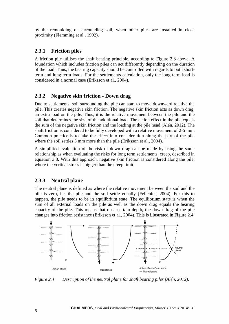
Neutral plane 2.3.3
The neutral plane is defined as where the relative movement between the soil and the
pile is zero, i.e. the pile and the soil settle equally (Fellenius, 2004). For this to
happen, the pile needs to be in equilibrium state. The equilibrium state is when the
sum of all external loads on the pile as well as the down drag equals the bearing
capacity of the pile. This means that on a certain depth, the down drag of the pile
changes into friction resistance (Eriksson et al., 2004). This is illustrated in Figure 2.4.
Figure 2.4 Description of the neutral plane for shaft bearing piles (Alén, 2012).
CHALMERS, Civil and Environmental Engineering, Master’s Thesis 2014:131 7
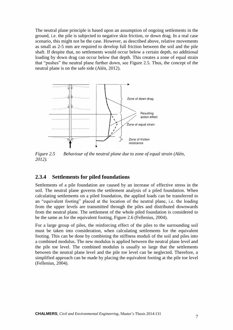
The neutral plane principle is based upon an assumption of ongoing settlements in the
ground, i.e. the pile is subjected to negative skin friction, or down drag. In a real case
scenario, this might not be the case. However, as described above, relative movements
as small as 2-5 mm are required to develop full friction between the soil and the pile
shaft. If despite that, no settlements would occur below a certain depth, no additional
loading by down drag can occur below that depth. This creates a zone of equal strain
that “pushes” the neutral plane further down, see Figure 2.5. Thus, the concept of the
neutral plane is on the safe side (Alén, 2012).
Figure 2.5 Behaviour of the neutral plane due to zone of equal strain (Alén,
2012).
Settlements for piled foundations 2.3.4
Settlements of a pile foundation are caused by an increase of effective stress in the
soil. The neutral plane governs the settlement analysis of a piled foundation. When
calculating settlements on a piled foundation, the applied loads can be transferred to
an “equivalent footing” placed at the location of the neutral plane, i.e. the loading
from the upper levels are transmitted through the piles and distributed downwards
from the neutral plane. The settlement of the whole piled foundation is considered to
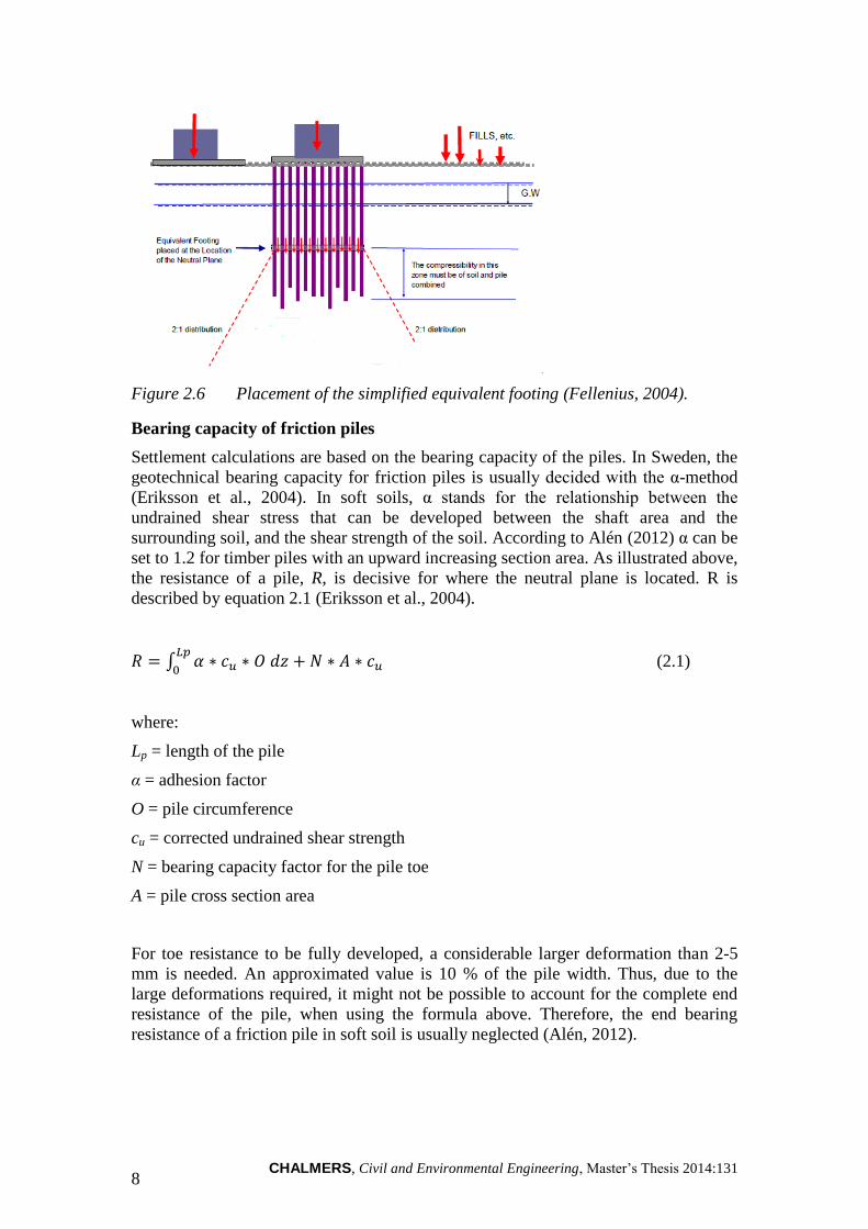
be the same as for the equivalent footing, Figure 2.6 (Fellenius, 2004).
For a large group of piles, the reinforcing effect of the piles to the surrounding soil
must be taken into consideration, when calculating settlements for the equivalent
footing. This can be done by combining the stiffness moduli of the soil and piles into
a combined modulus. The new modulus is applied between the neutral plane level and
the pile toe level. The combined modulus is usually so large that the settlements
between the neutral plane level and the pile toe level can be neglected. Therefore, a
simplified approach can be made by placing the equivalent footing at the pile toe level
(Fellenius, 2004).
CHALMERS, Civil and Environmental Engineering, Master’s Thesis 2014:131 8
Figure 2.6 Placement of the simplified equivalent footing (Fellenius, 2004).
Bearing capacity of friction piles
Settlement calculations are based on the bearing capacity of the piles. In Sweden, the
geotechnical bearing capacity for friction piles is usually decided with the α-method
(Eriksson et al., 2004). In soft soils, α stands for the relationship between the
undrained shear stress that can be developed between the shaft area and the
surrounding soil, and the shear strength of the soil. According to Alén (2012) α can be
set to 1.2 for timber piles with an upward increasing section area. As illustrated above,
the resistance of a pile, R, is decisive for where the neutral plane is located. R is
described by equation 2.1 (Eriksson et al., 2004).
∫
(2.1)
where:
Lp = length of the pile
α = adhesion factor
O = pile circumference
cu = corrected undrained shear strength
N = bearing capacity factor for the pile toe
A = pile cross section area
For toe resistance to be fully developed, a considerable larger deformation than 2-5
mm is needed. An approximated value is 10 % of the pile width. Thus, due to the
large deformations required, it might not be possible to account for the complete end
resistance of the pile, when using the formula above. Therefore, the end bearing
resistance of a friction pile in soft soil is usually neglected (Alén, 2012).

CHALMERS, Civil and Environmental Engineering, Master’s Thesis 2014:131 9
2.4 Composite foundation - Piled raft
According to Eriksson et al. (2004) there are three different design methods for piled
rafts:
The “conventional case”. Foundations where all load is carried by friction
piles. In a case like this, the piles have to acquire sufficient bearing capacity as
well as reduce the settlements.
Foundations where the load distribution is divided between the friction piles
and the contact pressure from the soil on a foundation slab. Used when the
weight of the excavated soil only covers part of the applied load. The piles
main function here is to reduce settlements. The creep pile principle can be
applied for such foundations.
Foundations where all applied load can be carried by the contact pressure
against the foundation slab. In such cases, the friction piles are placed under
concentrated loads and their primary function are to decrease the dimensions
of the overlying constructions, such as the foundation slab. This is suitable
when all applied loads can be compensated by excavating soil.
Most foundations constructed on clay are within the limits from a bearing capacity
perspective without the use of piles (Jedenby, 1986b). The main reason for adding pile
elements to the raft is usually not to carry the major part of the loads but to reduce
average and differential settlements (Kulhawy and Prakoso, 2001). Therefore, the
piles are designed to act both as soil reinforcing and settlement reducing elements, as
well as to take care of concentrated loads acting on the raft. The distribution and
number of piles is decided upon these criteria. This enables the design of the
foundation to be optimized and the number of piles to be reduced, which generally is
the most cost effective approach (Hansbo and Källström, 1983).
The load sharing mechanism of a piled raft, as well as its stiffness and resistance, is
regulated by the soil structure interactions between the load bearing components of
the foundation, i.e. the piles, the raft and the soil (Giretti, 2009). The raft is often
designed to carry loads of the same size as the preconsolidation pressure (Jendeby,
1986a).
As illustrated in Figure 2.7, a piled raft foundation can be assumed to have four kinds
of interactions. Each interaction is governed by the parameters of the three elements,
for example stiffness, shear strength of the soil, pile spacing and pile length. The pile-
soil and pile-raft interactions are described in earlier in this chapter. The pile-pile
interaction can be defined as additional settlements of a pile, caused by a loaded
adjacent pile, and the pile-raft interaction can be defined as additional settlement of
the raft caused by supporting piles (Nguyen, Jo and Kim, 2013).

CHALMERS, Civil and Environmental Engineering, Master’s Thesis 2014:131 10
Figure 2.7 The four different interactions of a piled-raft foundation (Katzenbach,
Gutberlet and Bachmann, 2007).
The creep pile principle 2.4.1
The use of a relatively high safety factor when designing a piled foundation could
result in a scenario where the surrounding soil settles more than the foundation, which
would mean that no contribution from contact pressure between soil and raft could be
accounted for. The principle of a piled raft foundation is to distribute the loads
between the raft and the piles. To achieve this, the design of the factor of safety of the
piles is close to unity, which means that the neutral plane is designed to be located at
or close to the bottom of the raft (Fellenius, 2004). With the piled raft method, the
piles can be designed to make the potential settlements of the foundation be the same
as the settlements of the surrounding soil. This is done through a better utilisation of
the piles, by designing them to be exposed of a load equal to their creep load, causing
a state of creep failure (Fredriksson and Rosén, 1988).
The design should ensure that the contact stress is uniformly distributed across the raft
(Fellenius, 2004). The ability of a construction to distribute forces horisontally is
especially governed by the stiffness of the construction (Eriksson et al., 2004). Since
there is pressure acting on the raft, it will generally have to be thicker and more
reinforced than in a conventional piling case.
The theory behind the principle is to take advantage of the compensation in effective
stress created by the excavated soil. A certain percentage (Q1) of the total applied
load (Q), can be carried without piles, due to the compensation. The remaining part of
the load (Q-Q1) has to be carried by the pile system. For example, if a raft can carry
80% of the load without causing substantial settlements, the piles has to carry the
remaining 20% of the load. Thus, the purpose of using the creep pile principle is to
maximize the pile capacity in order to control that a certain part of the load will be
carried by the raft. The pile spacing is chosen to regulate the amount of load carried
by piles (Hansbo and Jedenby, 1998).

CHALMERS, Civil and Environmental Engineering, Master’s Thesis 2014:131 11
The load-settlement behaviour for different design approaches, concerning a piled
raft, is presented in Figure 2.8. Curve 0 represents the behaviour of a raft acting alone.
Curve 1 represents the conventional design approach. Curve 2 illustrates the “creep
pile principle”, in which the piles are designed with a lower factor of safety. Curve 3
represents the use of full utilization of the piles at the design load, by strategically
placing the piles as settlement reducers. The reduction in number of piles for curve 2
and 3, results in a larger amount of load carried by the raft. Fewer piles results in a
more economical design (Poulos, 2001).
Figure 2.8 Load-settlement behaviour for a piled raft, comparing different design
approaches (Poulos, 2001).
2.5 Magnitude of allowable settlements for foundations on
soft cohesive soil
A settlement analysis should involve more than just an upper boundary. Both total
amount of settlements as well as differential settlements needs to be evaluated. The
magnitude of acceptable settlements varies with the size and type of structure
(Fellenius, 2006).
The differential settlement ratio is calculated as the difference in settlement of two
edges of a section, divided by the length between them. In Appendix E, allowable
settlement limits for structures, according to Holtz (1991), are presented. It underlines
that the settlement demands varies depending on the type of structure and its function.
CHALMERS, Civil and Environmental Engineering, Master’s Thesis 2014:131 12
3 Case study of Nordstaden 8:27
This chapter contains information about the case study building and its surroundings.
It also contains information about geotechnical conditions at the site, in form of
evaluations made from test documentation.
3.1 History of the area
The district Östra Nordstaden is situated north of Stora Hamnkanalen and east of
Östra Hamngatan and was earlier a district of emigrant hotels, storehouses and
brasseries. This is also the place where “Chalmer’s crafting school” once started in the
first half of the 19th century. Most of the buildings were from the late 18th or early
19th century. Since the 1970’s, this area is totally dominated by the shopping centre
Nordstan. (Fritz, 1997).
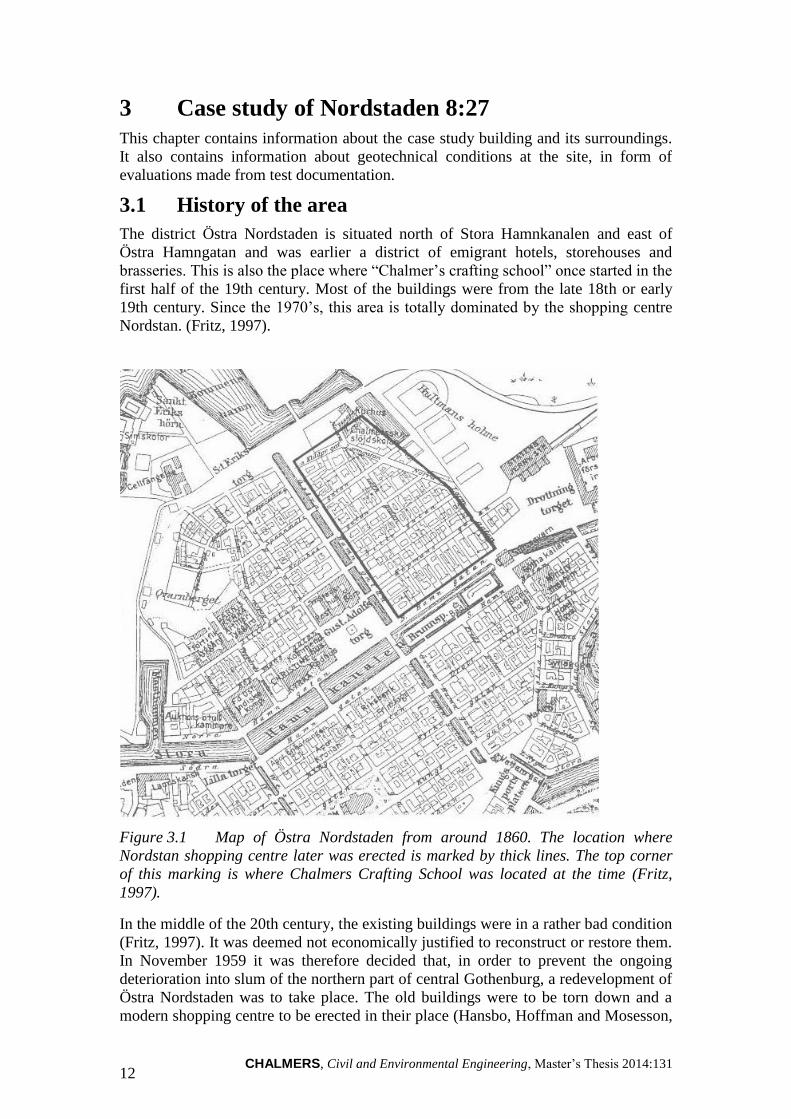
Figure 3.1 Map of Östra Nordstaden from around 1860. The location where
Nordstan shopping centre later was erected is marked by thick lines. The top corner
of this marking is where Chalmers Crafting School was located at the time (Fritz,
1997).
In the middle of the 20th century, the existing buildings were in a rather bad condition
(Fritz, 1997). It was deemed not economically justified to reconstruct or restore them.
In November 1959 it was therefore decided that, in order to prevent the ongoing
deterioration into slum of the northern part of central Gothenburg, a redevelopment of
Östra Nordstaden was to take place. The old buildings were to be torn down and a
modern shopping centre to be erected in their place (Hansbo, Hoffman and Mosesson,
CHALMERS, Civil and Environmental Engineering, Master’s Thesis 2014:131 13
1973). The first buildings, 1 and 2, were constructed during the years 1965-68, while
buildings 3 to 9 were constructed during the years 1970-76.
3.2 Geotechnical conditions
The geological data used for the case study of this thesis come from investigations
performed by AB Flygfältsbyrån and Jacobson & Widmark AB (J&W AB) in 1966,
during planning of the reconstruction. The tests consist of in-situ testings as Field
Vane Tests (FVT) and Cone Penetration Tests (CPT), as well as standard laboratory
tests, consisting of stepwise oedometer tests and fall cone tests. Oedometer tests were
performed on soil from two boreholes, 1 and 17b, in the area and down two a depth of
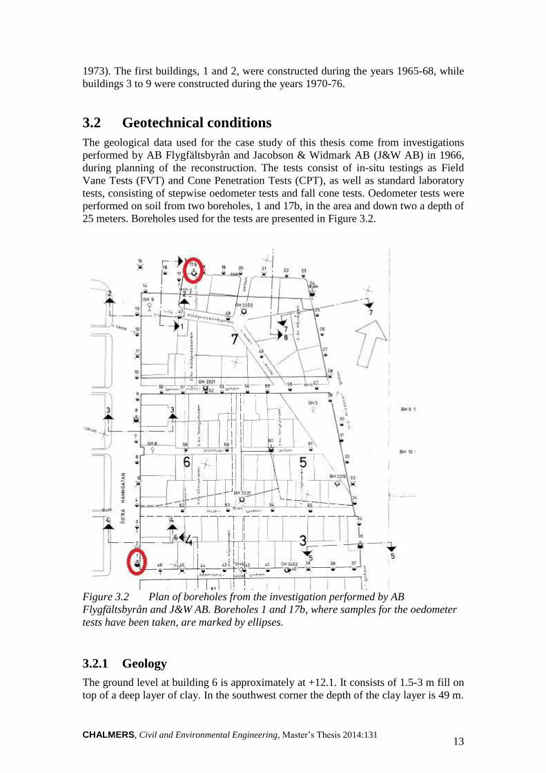
25 meters. Boreholes used for the tests are presented in Figure 3.2.
Figure 3.2 Plan of boreholes from the investigation performed by AB
Flygfältsbyrån and J&W AB. Boreholes 1 and 17b, where samples for the oedometer
tests have been taken, are marked by ellipses.
Geology 3.2.1
The ground level at building 6 is approximately at +12.1. It consists of 1.5-3 m fill on
top of a deep layer of clay. In the southwest corner the depth of the clay layer is 49 m.

CHALMERS, Civil and Environmental Engineering, Master’s Thesis 2014:131 14
Below there is a 2 m thick layer of frictional soil resting on the bedrock. In the other
three corners the clay and friction soil layers has a thickness of approximately 90 and
10 m respectively. Sampling of soil has been made to a depth of 40 m (Svensson,
1993).
Hydrogeological conditions 3.2.2
The mean groundwater level for the area is approximately at level +10.1. There is a
hydrostatic overpressure of 20-30 kPa at a depth of 20 m. There is however no
information on what level this overpressure starts (Svensson, 1993).
Soil properties - parameter evaluation 3.2.3
This chapter presents parameters evaluated from the obtained tests as well as
assumptions made regarding other parameters that will be of importance for this
thesis.
Unit weight - γsoil
The volume weight is uniform with depth and has an approximate value of 1.6 t/m3.
The data is transformed into unit weight, γsoil [kN/m3]. A graph of the unit weight
plotted versus level can be seen in Appendix C.
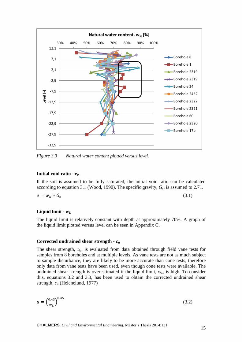
Natural water content - wN
The natural water content, wN, is obtained from standard tests in laboratory, and is
plotted versus level in Figure 3.3. The graph indicates a homogeneous layer of clay,
apart from the highlighted area, which implies that there is a section with higher water
content.
CHALMERS, Civil and Environmental Engineering, Master’s Thesis 2014:131 15
Figure 3.3 Natural water content plotted versus level.
Initial void ratio - e0
If the soil is assumed to be fully saturated, the initial void ratio can be calculated
according to equation 3.1 (Wood, 1990). The specific gravity, Gs, is assumed to 2.71.
(3.1)
Liquid limit - wL
The liquid limit is relatively constant with depth at approximately 70%. A graph of
the liquid limit plotted versus level can be seen in Appendix C.
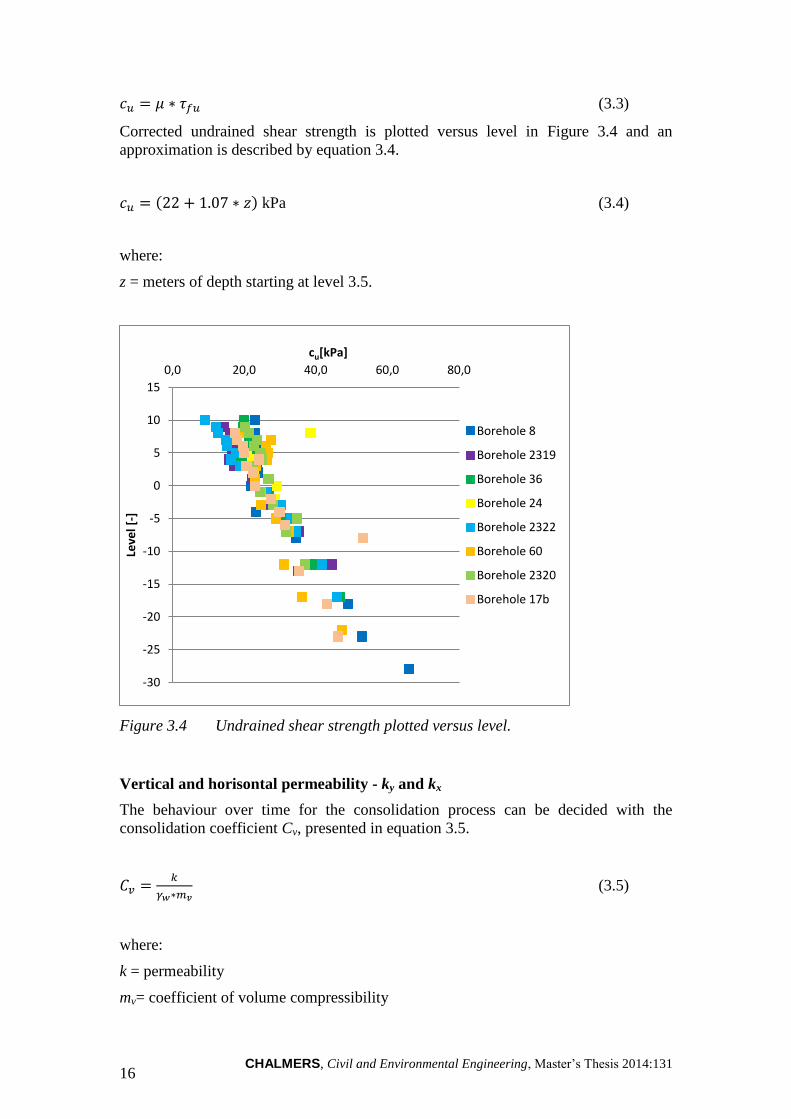
Corrected undrained shear strength - cu
The shear strength, τfu, is evaluated from data obtained through field vane tests for
samples from 8 boreholes and at multiple levels. As vane tests are not as much subject
to sample disturbance, they are likely to be more accurate than cone tests, therefore
only data from vane tests have been used, even though cone tests were available. The
undrained shear strength is overestimated if the liquid limit, wL, is high. To consider
this, equations 3.2 and 3.3, has been used to obtain the corrected undrained shear
strength, cu (Helenelund, 1977).
(
)
(3.2)
-32,9
-27,9
-22,9
-17,9
-12,9
-7,9
-2,9
2,1
7,1
12,1
30% 40% 50% 60% 70% 80% 90% 100%Le
vel [
-]
Natural water content, wN [%]
Borehole 8
Borehole 1
Borehole 2319
Borehole 2319
Borehole 24
Borehole 2452
Borehole 2322
Borehole 2321
Borehole 60
Borehole 2320
Borehole 17b
CHALMERS, Civil and Environmental Engineering, Master’s Thesis 2014:131 16
(3.3)
Corrected undrained shear strength is plotted versus level in Figure 3.4 and an
approximation is described by equation 3.4.
( ) kPa (3.4)
where:
z = meters of depth starting at level 3.5.
Figure 3.4 Undrained shear strength plotted versus level.
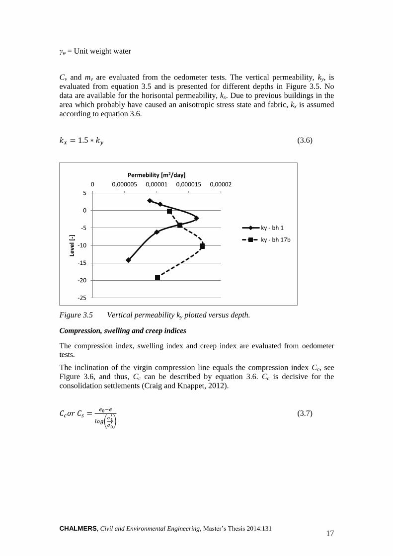
Vertical and horisontal permeability - ky and kx
The behaviour over time for the consolidation process can be decided with the
consolidation coefficient Cv, presented in equation 3.5.
(3.5)
where:
k = permeability
mv= coefficient of volume compressibility
-30
-25
-20
-15
-10
-5
0
5
10
15
0,0 20,0 40,0 60,0 80,0
Leve
l [-]
cu[kPa]
Borehole 8
Borehole 2319
Borehole 36
Borehole 24
Borehole 2322
Borehole 60
Borehole 2320
Borehole 17b
CHALMERS, Civil and Environmental Engineering, Master’s Thesis 2014:131 17
γw = Unit weight water
Cv and mv are evaluated from the oedometer tests. The vertical permeability, ky, is
evaluated from equation 3.5 and is presented for different depths in Figure 3.5. No
data are available for the horisontal permeability, kx. Due to previous buildings in the
area which probably have caused an anisotropic stress state and fabric, kx is assumed
according to equation 3.6.
(3.6)
Figure 3.5 Vertical permeability ky plotted versus depth.
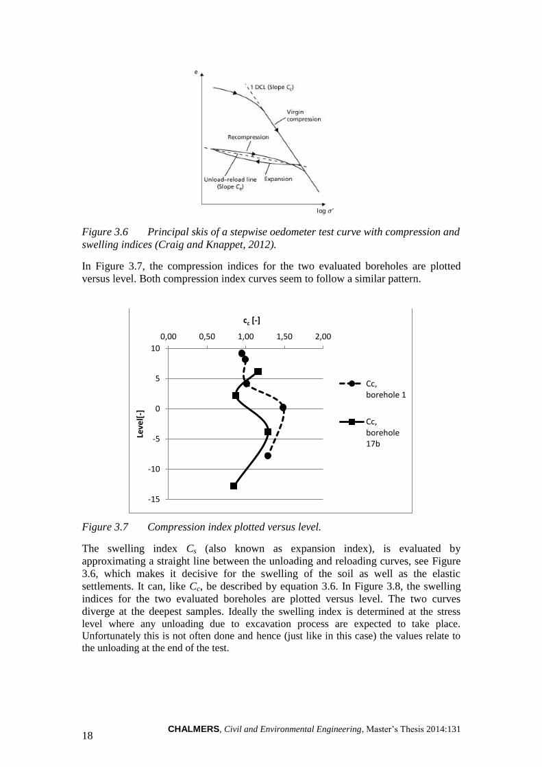
Compression, swelling and creep indices
The compression index, swelling index and creep index are evaluated from oedometer
tests.
The inclination of the virgin compression line equals the compression index Cc, see
Figure 3.6, and thus, Cc can be described by equation 3.6. Cc is decisive for the
consolidation settlements (Craig and Knappet, 2012).
(
)
(3.7)
-25
-20
-15
-10
-5
0
5
0 0,000005 0,00001 0,000015 0,00002
Leve
l [-]
Permebility [m2/day]
ky - bh 1
ky - bh 17b
CHALMERS, Civil and Environmental Engineering, Master’s Thesis 2014:131 18
Figure 3.6 Principal skis of a stepwise oedometer test curve with compression and
swelling indices (Craig and Knappet, 2012).
In Figure 3.7, the compression indices for the two evaluated boreholes are plotted
versus level. Both compression index curves seem to follow a similar pattern.
Figure 3.7 Compression index plotted versus level.
The swelling index Cs (also known as expansion index), is evaluated by
approximating a straight line between the unloading and reloading curves, see Figure
3.6, which makes it decisive for the swelling of the soil as well as the elastic
settlements. It can, like Cc, be described by equation 3.6. In Figure 3.8, the swelling
indices for the two evaluated boreholes are plotted versus level. The two curves
diverge at the deepest samples. Ideally the swelling index is determined at the stress
level where any unloading due to excavation process are expected to take place.
Unfortunately this is not often done and hence (just like in this case) the values relate to
the unloading at the end of the test.
-15
-10
-5
0
5
10
0,00 0,50 1,00 1,50 2,00
Leve
l[-]
cc [-]
Cc,borehole 1
Cc,borehole17b

CHALMERS, Civil and Environmental Engineering, Master’s Thesis 2014:131 19
Figure 3.8 Swelling index plotted versus level
Creep index
The rate of secondary compression, or creep index Cα, is evaluated as the inclination
of the final part of the semi-logarithmic graph in figure Figure 3.9.
Figure 3.9 Oedometer test plotted as logarithmic time versus strain/void ratio
(Olsson, 2010).
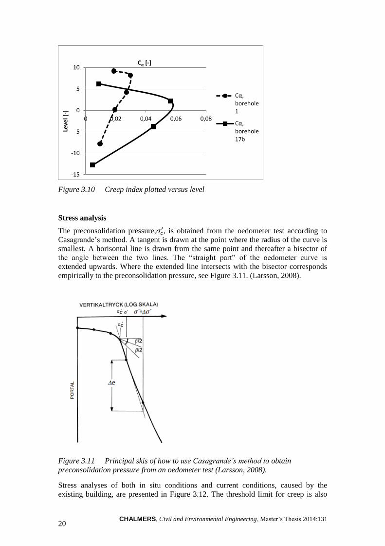
In Figure 3.10 the creep index for the two evaluated boreholes are plotted versus
level. Both creep index curves seem to have similar patterns, but with the data from
borehole 17b reaching higher values.
-15
-10
-5
0
5
10
0 0,05 0,1 0,15
Leve
l [-]
cs [-]
Cs, borehole1
Cs, borehole17b
CHALMERS, Civil and Environmental Engineering, Master’s Thesis 2014:131 20
Figure 3.10 Creep index plotted versus level
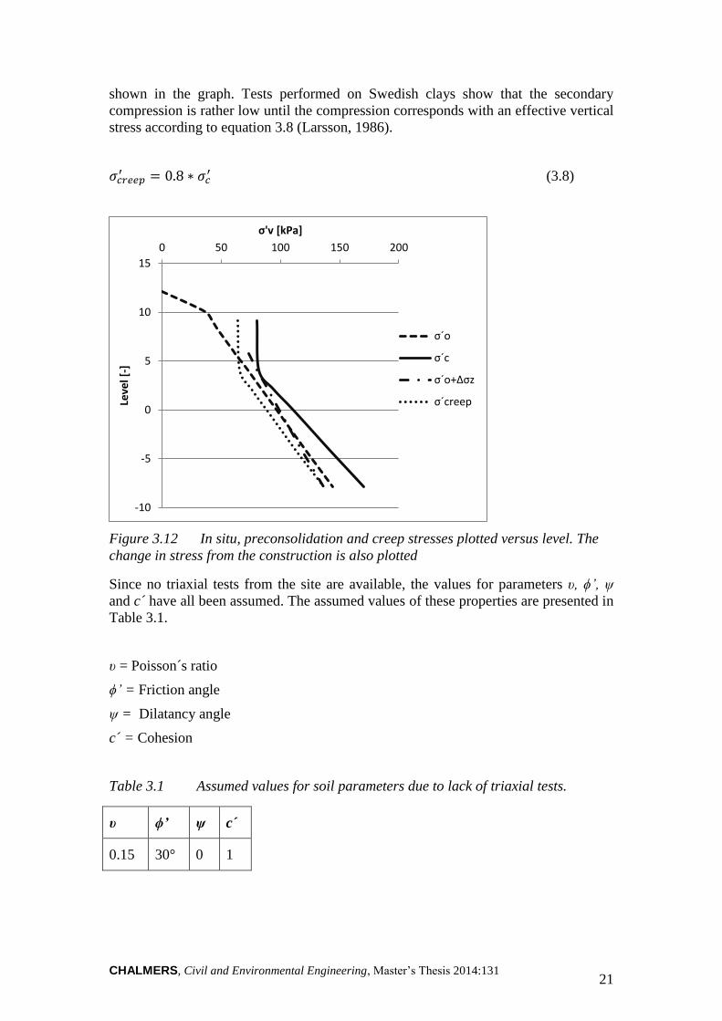
Stress analysis
The preconsolidation pressure, , is obtained from the oedometer test according to
Casagrande’s method. A tangent is drawn at the point where the radius of the curve is
smallest. A horisontal line is drawn from the same point and thereafter a bisector of
the angle between the two lines. The “straight part” of the oedometer curve is
extended upwards. Where the extended line intersects with the bisector corresponds
empirically to the preconsolidation pressure, see Figure 3.11. (Larsson, 2008).
Figure 3.11 Principal skis of how to use Casagrande’s method to obtain
preconsolidation pressure from an oedometer test (Larsson, 2008).
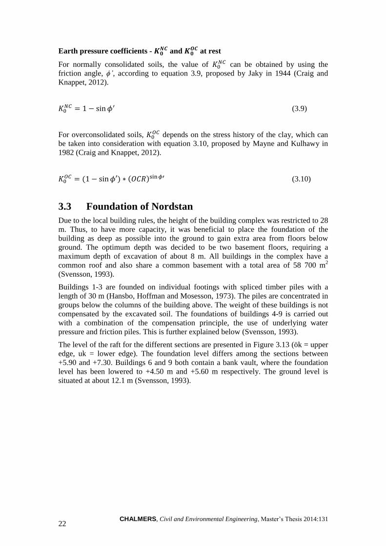
Stress analyses of both in situ conditions and current conditions, caused by the
existing building, are presented in Figure 3.12. The threshold limit for creep is also
-15
-10
-5
0
5
10
0 0,02 0,04 0,06 0,08
Leve
l [-]
Cα [-]
Cα, borehole 1
Cα, borehole 17b
CHALMERS, Civil and Environmental Engineering, Master’s Thesis 2014:131 21
shown in the graph. Tests performed on Swedish clays show that the secondary
compression is rather low until the compression corresponds with an effective vertical
stress according to equation 3.8 (Larsson, 1986).
(3.8)
Figure 3.12 In situ, preconsolidation and creep stresses plotted versus level. The
change in stress from the construction is also plotted
Since no triaxial tests from the site are available, the values for parameters υ, ϕ’, ψ
and c´ have all been assumed. The assumed values of these properties are presented in
Table 3.1.
υ = Poisson´s ratio
ϕ’ = Friction angle
ψ = Dilatancy angle
c´ = Cohesion
Table 3.1 Assumed values for soil parameters due to lack of triaxial tests.
υ ϕ’ ψ c´
0.15 30° 0 1
-10
-5
0
5
10
15
0 50 100 150 200
Leve
l [-]
σ'v [kPa]
σ´o
σ´c
σ´o+Δσz
σ´creep
CHALMERS, Civil and Environmental Engineering, Master’s Thesis 2014:131 22
Earth pressure coefficients - and
at rest
For normally consolidated soils, the value of can be obtained by using the
friction angle, ϕ’, according to equation 3.9, proposed by Jaky in 1944 (Craig and
Knappet, 2012).
(3.9)
For overconsolidated soils, depends on the stress history of the clay, which can
be taken into consideration with equation 3.10, proposed by Mayne and Kulhawy in
1982 (Craig and Knappet, 2012).
( ) ( ) (3.10)
3.3 Foundation of Nordstan
Due to the local building rules, the height of the building complex was restricted to 28
m. Thus, to have more capacity, it was beneficial to place the foundation of the
building as deep as possible into the ground to gain extra area from floors below
ground. The optimum depth was decided to be two basement floors, requiring a
maximum depth of excavation of about 8 m. All buildings in the complex have a
common roof and also share a common basement with a total area of 58 700 m2
(Svensson, 1993).
Buildings 1-3 are founded on individual footings with spliced timber piles with a
length of 30 m (Hansbo, Hoffman and Mosesson, 1973). The piles are concentrated in
groups below the columns of the building above. The weight of these buildings is not
compensated by the excavated soil. The foundations of buildings 4-9 is carried out
with a combination of the compensation principle, the use of underlying water
pressure and friction piles. This is further explained below (Svensson, 1993).
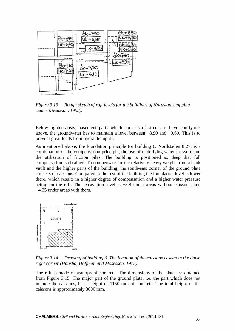
The level of the raft for the different sections are presented in Figure 3.13 (ök = upper
edge, uk = lower edge). The foundation level differs among the sections between
+5.90 and +7.30. Buildings 6 and 9 both contain a bank vault, where the foundation
level has been lowered to +4.50 m and +5.60 m respectively. The ground level is
situated at about 12.1 m (Svensson, 1993).
CHALMERS, Civil and Environmental Engineering, Master’s Thesis 2014:131 23
Figure 3.13 Rough sketch of raft levels for the buildings of Nordstan shopping
centre (Svensson, 1993).
Below lighter areas, basement parts which consists of streets or have courtyards
above, the groundwater has to maintain a level between +8.90 and +9.60. This is to
prevent great loads from hydraulic uplift.
As mentioned above, the foundation principle for building 6, Nordstaden 8:27, is a
combination of the compensation principle, the use of underlying water pressure and
the utilisation of friction piles. The building is positioned so deep that full
compensation is obtained. To compensate for the relatively heavy weight from a bank
vault and the higher parts of the building, the south-east corner of the ground plate
consists of caissons. Compared to the rest of the building the foundation level is lower
there, which results in a higher degree of compensation and a higher water pressure
acting on the raft. The excavation level is +5.8 under areas without caissons, and
+4.25 under areas with them.
Figure 3.14 Drawing of building 6. The location of the caissons is seen in the down
right corner (Hansbo, Hoffman and Mosesson, 1973).
The raft is made of waterproof concrete. The dimensions of the plate are obtained
from Figure 3.15. The major part of the ground plate, i.e. the part which does not
include the caissons, has a height of 1150 mm of concrete. The total height of the
caissons is approximately 3000 mm.

CHALMERS, Civil and Environmental Engineering, Master’s Thesis 2014:131 24
Figure 3.15 Details of the raft including underlying material (concrete K75, plastic
foil, gravel (2 – 20 mm), concrete K75, gravel, clay). All dimensions are given in
[mm].
Since the groundwater level is located above the foundation level, the loads from the
building is partly carried by water pressure, acting on the raft from below. In order to
maintain a high groundwater pressure below heavier parts and reduce it below lighter
parts, groundwater conditions are regulated. Beneath the raft there is a 10 cm thick
permeable layer of gravel. Wooden sheet piles create watertight sections and separate
the ground beneath the object, and even parts within the object itself. Because of this
the level of the groundwater table varies between different areas. Each encircled area
has a regulated water level, controlled by pumps, which automatically handles refill
and overflow when needed. There are four different watertight sections beneath
building 6. Their positions are presented in Figure 3.16.

CHALMERS, Civil and Environmental Engineering, Master’s Thesis 2014:131 25
Figure 3.16 Water reservoirs below building 6. The borders of the four different
reservoirs are marked with thicker red lines and adjacent names.
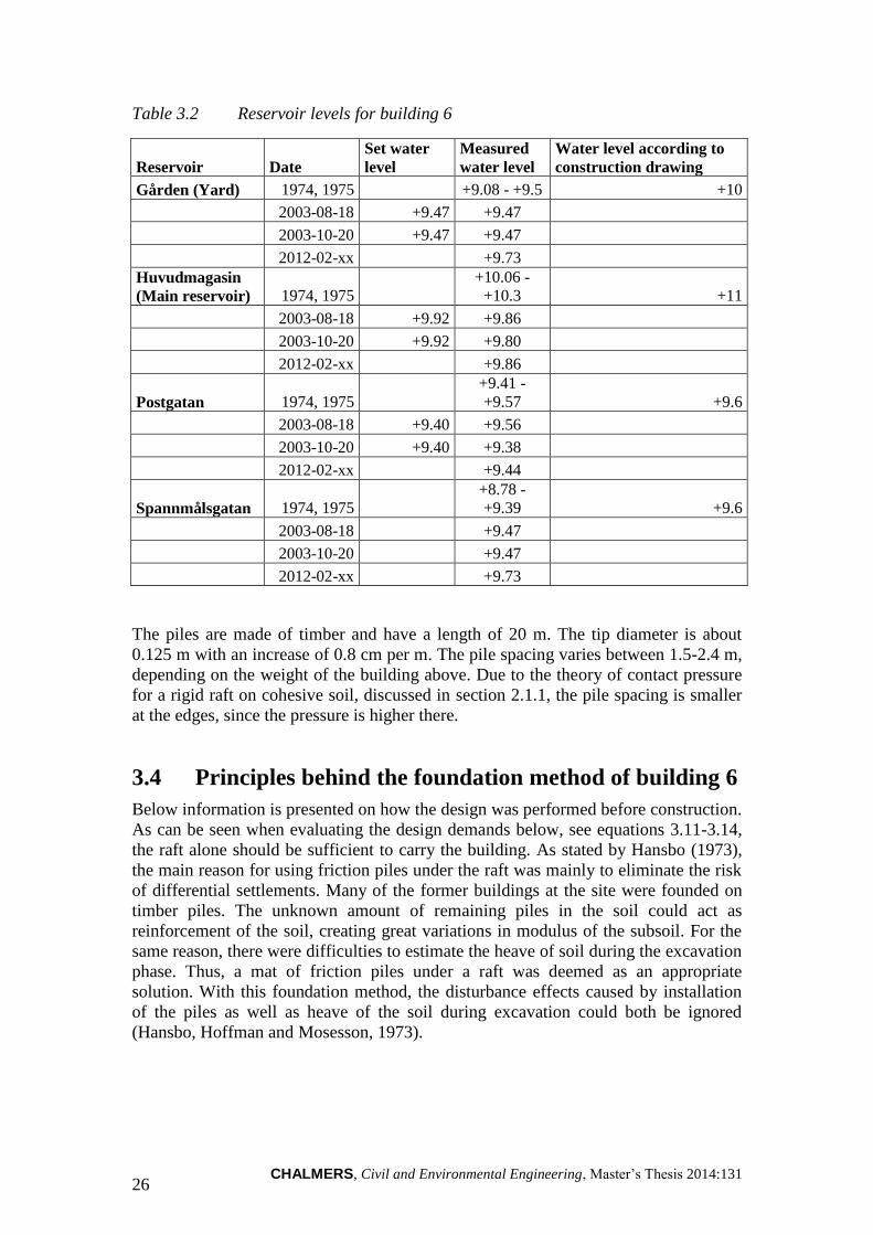
As can be seen in Table 3.2, there is a difference between the level set as a limit in the
design and the measured water level in the main reservoir. This is due to problems in
maintaining the set level. The owners could not tell for how long the level has been
this low2.
2 Torbjörn Petterson, technical manager at Vasakronan, interviewed 14-02-20
CHALMERS, Civil and Environmental Engineering, Master’s Thesis 2014:131 26
Table 3.2 Reservoir levels for building 6
Reservoir Date
Set water
level
Measured
water level
Water level according to
construction drawing
Gården (Yard) 1974, 1975 +9.08 - +9.5 +10
2003-08-18 +9.47 +9.47
2003-10-20 +9.47 +9.47
2012-02-xx +9.73
Huvudmagasin
(Main reservoir) 1974, 1975
+10.06 -
+10.3 +11
2003-08-18 +9.92 +9.86
2003-10-20 +9.92 +9.80
2012-02-xx +9.86
Postgatan 1974, 1975
+9.41 -
+9.57 +9.6
2003-08-18 +9.40 +9.56
2003-10-20 +9.40 +9.38
2012-02-xx +9.44
Spannmålsgatan 1974, 1975
+8.78 -
+9.39 +9.6
2003-08-18 +9.47
2003-10-20 +9.47
2012-02-xx +9.73
The piles are made of timber and have a length of 20 m. The tip diameter is about
0.125 m with an increase of 0.8 cm per m. The pile spacing varies between 1.5-2.4 m,
depending on the weight of the building above. Due to the theory of contact pressure
for a rigid raft on cohesive soil, discussed in section 2.1.1, the pile spacing is smaller
at the edges, since the pressure is higher there.
3.4 Principles behind the foundation method of building 6
Below information is presented on how the design was performed before construction.
As can be seen when evaluating the design demands below, see equations 3.11-3.14,
the raft alone should be sufficient to carry the building. As stated by Hansbo (1973),
the main reason for using friction piles under the raft was mainly to eliminate the risk
of differential settlements. Many of the former buildings at the site were founded on
timber piles. The unknown amount of remaining piles in the soil could act as
reinforcement of the soil, creating great variations in modulus of the subsoil. For the
same reason, there were difficulties to estimate the heave of soil during the excavation
phase. Thus, a mat of friction piles under a raft was deemed as an appropriate
solution. With this foundation method, the disturbance effects caused by installation
of the piles as well as heave of the soil during excavation could both be ignored
(Hansbo, Hoffman and Mosesson, 1973).
CHALMERS, Civil and Environmental Engineering, Master’s Thesis 2014:131 27
The design demands which the foundation were based on are presented below:
1. (3.11)
2.
(3.12)
3.
(3.13)
4.
(3.14)
where:
= load from the new building
= uplifting water pressure
= weight of excavated soil
= bearing capacity for the ground
= bearing capacity of the piles/area per pile
Since the bearing capacity of the piles is divided by the area covered by each pile to
obtain qpiles, the pile spacing was designed to obtain the safety factor of 2.
According to Hansbo, this was the first time foundation design was based on
interactivity between friction piles and pressure against the raft. The safety factor used
against failure according to conventional methods at the time was set to three. In this
case, which can be seen in demands 3 and 4 above, a safety factor of two was used.
Thus, the foundation of Nordstan can be seen as an introduction to the creep pile
principle, implementing a better utilisation of the piles3.
Bearing capacity of the soil 3.4.1
During the design of the foundation the bearing capacity of the soil was calculated
with equation 3.15, according to Svensk Byggnorm 67 (Statens planverk, 1968).
(
) (
) (3.15)
if D/B ≤ 2.5
where:
D = depth of raft below closest adjacent surface
B = width of raft
L = length of raft
= undrained shear strength of the soil
= unit weight of the soil
3 Sven Hansbo, Professor Emeritus, interviewed 14-02-24

CHALMERS, Civil and Environmental Engineering, Master’s Thesis 2014:131 28
D was chosen as zero. was set to its minimum value of 2.5 MP/m2. (2.5 MP/m
2
was the minimum shear strength from the parameter evaluation made in 1966, where
correction factor of shear strength was not considered). The bearing capacity was
calculated to 5.1 MP/m2 (approximately 51 kPa).
Figure 3.17 Definitions of D and B for equation 3.15 (Statens planverk, 1968).
Bearing capacity of the piles 3.4.2
During the design of the foundation the bearing capacity of the piles was calculated
with equations 3.16 – 3.20, according to Pålnormer sbn-n 23:6. The equation only
takes the shaft resistance into consideration and is based on Figure 3.18. It should be
noted that values in the figure does not consider the building in the case study, but the
principle however is accurate.
(3.16)
(3.17)
∫
(3.18)
( ) (3.19)
(3.20)
where:
R = bearing capacity of pile
Ri = bearing capacity of pile part i
di = diameter at pile part i
upile = expression for circumference of lower pile part in Figure 3.18
ui = circumference at pile part i
Lpilei = length of pile part i
= undrained shear strength of the soil
CHALMERS, Civil and Environmental Engineering, Master’s Thesis 2014:131 29
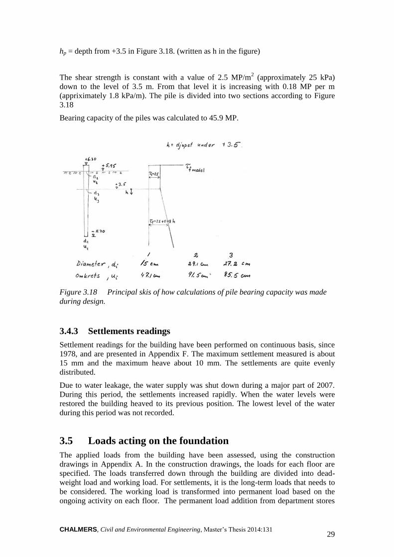
hp = depth from +3.5 in Figure 3.18. (written as h in the figure)
The shear strength is constant with a value of 2.5 MP/m2 (approximately 25 kPa)
down to the level of 3.5 m. From that level it is increasing with 0.18 MP per m
(appriximately 1.8 kPa/m). The pile is divided into two sections according to Figure
3.18
Bearing capacity of the piles was calculated to 45.9 MP.
Figure 3.18 Principal skis of how calculations of pile bearing capacity was made
during design.
Settlements readings 3.4.3
Settlement readings for the building have been performed on continuous basis, since
1978, and are presented in Appendix F. The maximum settlement measured is about
15 mm and the maximum heave about 10 mm. The settlements are quite evenly
distributed.
Due to water leakage, the water supply was shut down during a major part of 2007.
During this period, the settlements increased rapidly. When the water levels were
restored the building heaved to its previous position. The lowest level of the water
during this period was not recorded.
3.5 Loads acting on the foundation
The applied loads from the building have been assessed, using the construction
drawings in Appendix A. In the construction drawings, the loads for each floor are
specified. The loads transferred down through the building are divided into dead-
weight load and working load. For settlements, it is the long-term loads that needs to
be considered. The working load is transformed into permanent load based on the
ongoing activity on each floor. The permanent load addition from department stores
CHALMERS, Civil and Environmental Engineering, Master’s Thesis 2014:131 30
can be approximated as 60% of their working load, whereas 30 % percent of the
office load is considered as permanent load4. When the building was erected, the three
lower floors were used both as department stores and offices, in this thesis, they are
considered as department stores. The rest of the floors were used as offices, which
they also are considered to be in this thesis.
The facade consists of lightweight material (Gustafsson et al., n.d.). Therefore, the
load contribution from the facade is considered to be negligible. The load contribution
from pillars is approximated as 10 kN per floor. This is considered to be included in
the dead weight of each floor. The snow load is neglected due to the long-term
perspective4. The loads are summarized for each pillar, and is presented in Appendix
B.
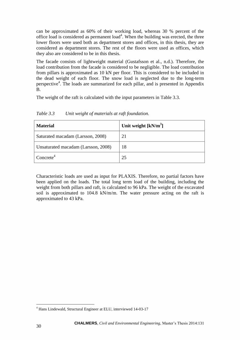
The weight of the raft is calculated with the input parameters in Table 3.3.
Table 3.3 Unit weight of materials at raft foundation.
Material Unit weight [kN/m3]
Saturated macadam (Larsson, 2008) 21
Unsaturated macadam (Larsson, 2008) 18
Concrete4 25
Characteristic loads are used as input for PLAXIS. Therefore, no partial factors have
been applied on the loads. The total long term load of the building, including the
weight from both pillars and raft, is calculated to 96 kPa. The weight of the excavated
soil is approximated to 104.8 kN/m/m. The water pressure acting on the raft is
approximated to 43 kPa.
4 Hans Lindewald, Structural Engineer at ELU, interviewed 14-03-17
CHALMERS, Civil and Environmental Engineering, Master’s Thesis 2014:131 31
4 Numerical analyses. Modelling in PLAXIS 2D
This chapter contains information about the finite element computer software
PLAXIS 2D.
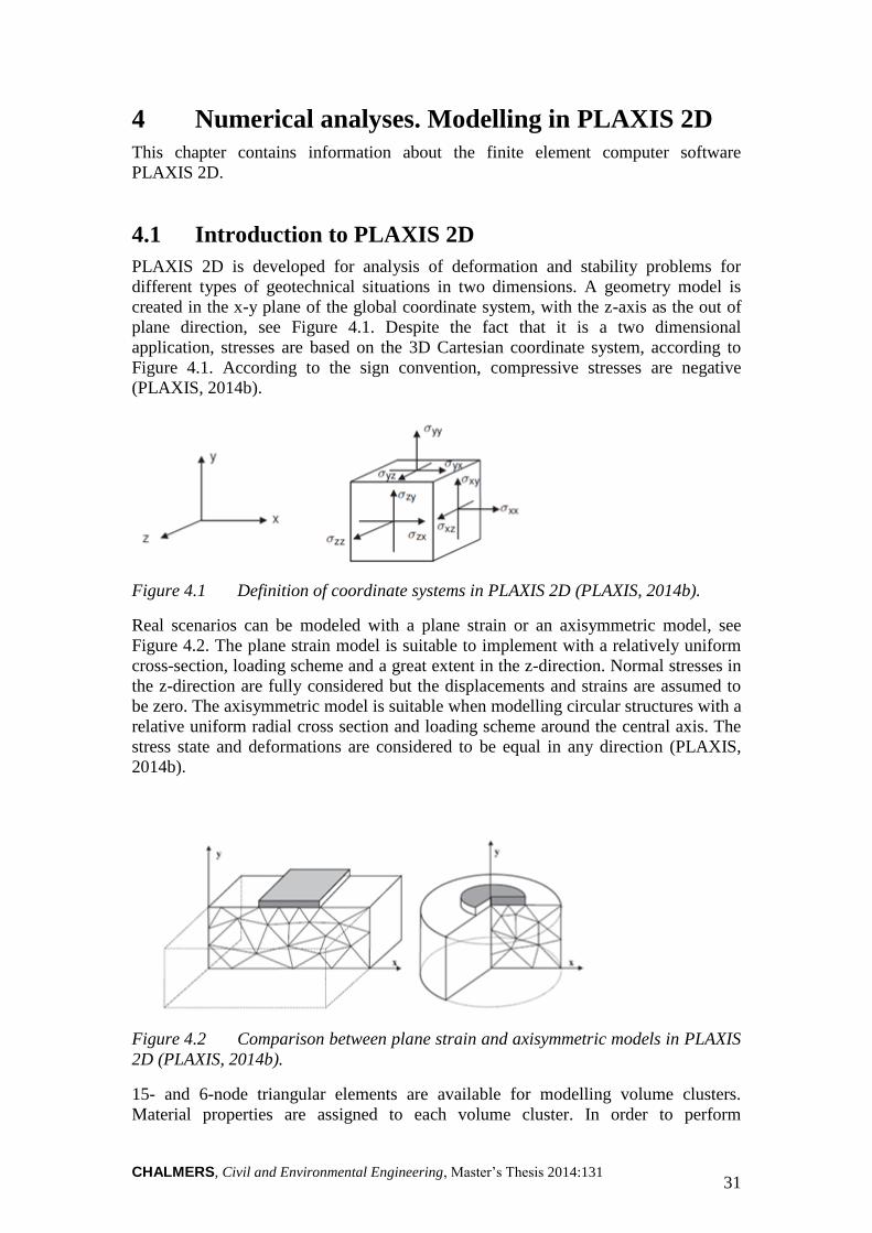
4.1 Introduction to PLAXIS 2D
PLAXIS 2D is developed for analysis of deformation and stability problems for
different types of geotechnical situations in two dimensions. A geometry model is
created in the x-y plane of the global coordinate system, with the z-axis as the out of
plane direction, see Figure 4.1. Despite the fact that it is a two dimensional
application, stresses are based on the 3D Cartesian coordinate system, according to
Figure 4.1. According to the sign convention, compressive stresses are negative
(PLAXIS, 2014b).
Figure 4.1 Definition of coordinate systems in PLAXIS 2D (PLAXIS, 2014b).
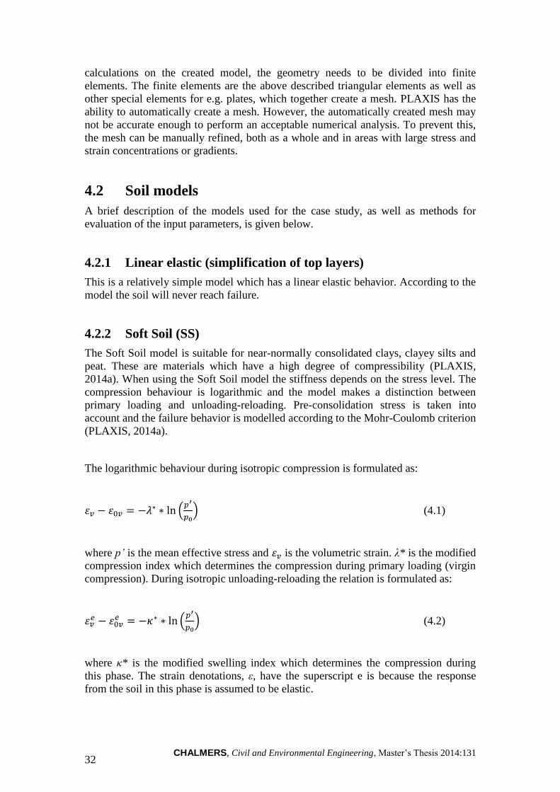
Real scenarios can be modeled with a plane strain or an axisymmetric model, see
Figure 4.2. The plane strain model is suitable to implement with a relatively uniform
cross-section, loading scheme and a great extent in the z-direction. Normal stresses in
the z-direction are fully considered but the displacements and strains are assumed to
be zero. The axisymmetric model is suitable when modelling circular structures with a
relative uniform radial cross section and loading scheme around the central axis. The
stress state and deformations are considered to be equal in any direction (PLAXIS,
2014b).
Figure 4.2 Comparison between plane strain and axisymmetric models in PLAXIS
2D (PLAXIS, 2014b).
15- and 6-node triangular elements are available for modelling volume clusters.
Material properties are assigned to each volume cluster. In order to perform
CHALMERS, Civil and Environmental Engineering, Master’s Thesis 2014:131 32
calculations on the created model, the geometry needs to be divided into finite
elements. The finite elements are the above described triangular elements as well as
other special elements for e.g. plates, which together create a mesh. PLAXIS has the
ability to automatically create a mesh. However, the automatically created mesh may
not be accurate enough to perform an acceptable numerical analysis. To prevent this,
the mesh can be manually refined, both as a whole and in areas with large stress and
strain concentrations or gradients.
4.2 Soil models
A brief description of the models used for the case study, as well as methods for
evaluation of the input parameters, is given below.
Linear elastic (simplification of top layers) 4.2.1
This is a relatively simple model which has a linear elastic behavior. According to the
model the soil will never reach failure.
Soft Soil (SS) 4.2.2
The Soft Soil model is suitable for near-normally consolidated clays, clayey silts and
peat. These are materials which have a high degree of compressibility (PLAXIS,
2014a). When using the Soft Soil model the stiffness depends on the stress level. The
compression behaviour is logarithmic and the model makes a distinction between
primary loading and unloading-reloading. Pre-consolidation stress is taken into
account and the failure behavior is modelled according to the Mohr-Coulomb criterion
(PLAXIS, 2014a).
The logarithmic behaviour during isotropic compression is formulated as:
(
) (4.1)
where p’ is the mean effective stress and is the volumetric strain. λ* is the modified
compression index which determines the compression during primary loading (virgin
compression). During isotropic unloading-reloading the relation is formulated as:
(
) (4.2)
where κ* is the modified swelling index which determines the compression during
this phase. The strain denotations, ε, have the superscript e is because the response
from the soil in this phase is assumed to be elastic.

CHALMERS, Civil and Environmental Engineering, Master’s Thesis 2014:131 33
Soft Soil model parameter evaluation
The modified compression and swelling indices, λ* and κ*, are evaluated from triaxial
tests. The modified compression and swelling indices can be obtained from a plot of
the logarithmic mean effective stress, p’, as a function of the volumetric strain, .
The first as the slope of the primary loading line and the latter as the slope of the
unloading-reloading line, see Figure 4.3.
Figure 4.3 Definitions of indices λ* and κ* (PLAXIS, 2014a).
These parameters can also be obtained from a one-dimensional oedometer test since
there is a relationship between λ*/κ*, and the parameters for one dimensional
compression and recompression Cc/Cs (PLAXIS, 2014a). In PLAXIS either could be
used as input value. Since only oedometer tests were available for this project
parameters Cc and Cs were evaluated and then transformed by using relationships
described below.
Modified compression index, λ*
The modified compression index λ* is obtained from the relationship with the
compression index, Cc, in equation 4.3 (PLAXIS, 2014a).
( ) (4.3)
Modified swelling index, κ*
The modified swelling index, κ*, is obtained from the relationship with the swelling
index, Cs, in equation 4.4 (PLAXIS, 2014a).
( ) (4.4)
Soft Soil Creep (SSC) 4.2.3
While the Soft Soil model is a suitable tool for modeling clays, it does not consider
the secondary compression (creep). The parameters and principles of the both models
CHALMERS, Civil and Environmental Engineering, Master’s Thesis 2014:131 34
coincide well with each other apart from the modified creep index, µ*, which takes
the time aspect into consideration (PLAXIS, 2014a).
Similar to the Soft Soil model, the Soft Soil Creep model distinguish between primary
loading and unloading/reloading. The difference is that for the Soft Soil Creep model,
the limit between the two loading states is not only determined by the maximum stress
state that has been reached in the past, but also by the time aspect (PLAXIS, 2014a).
The Soft Soil Creep model assumes a reference time, τ, of 1 day, which cannot be
altered. This is to be used in conjunction with a preconsolidation pressure
corresponding to 24 hours load step. For other load/strain rates, the input value of
OCR or POP needs to be scaled accordingly (Leoni, Karstunen and Vermeer, 2008).
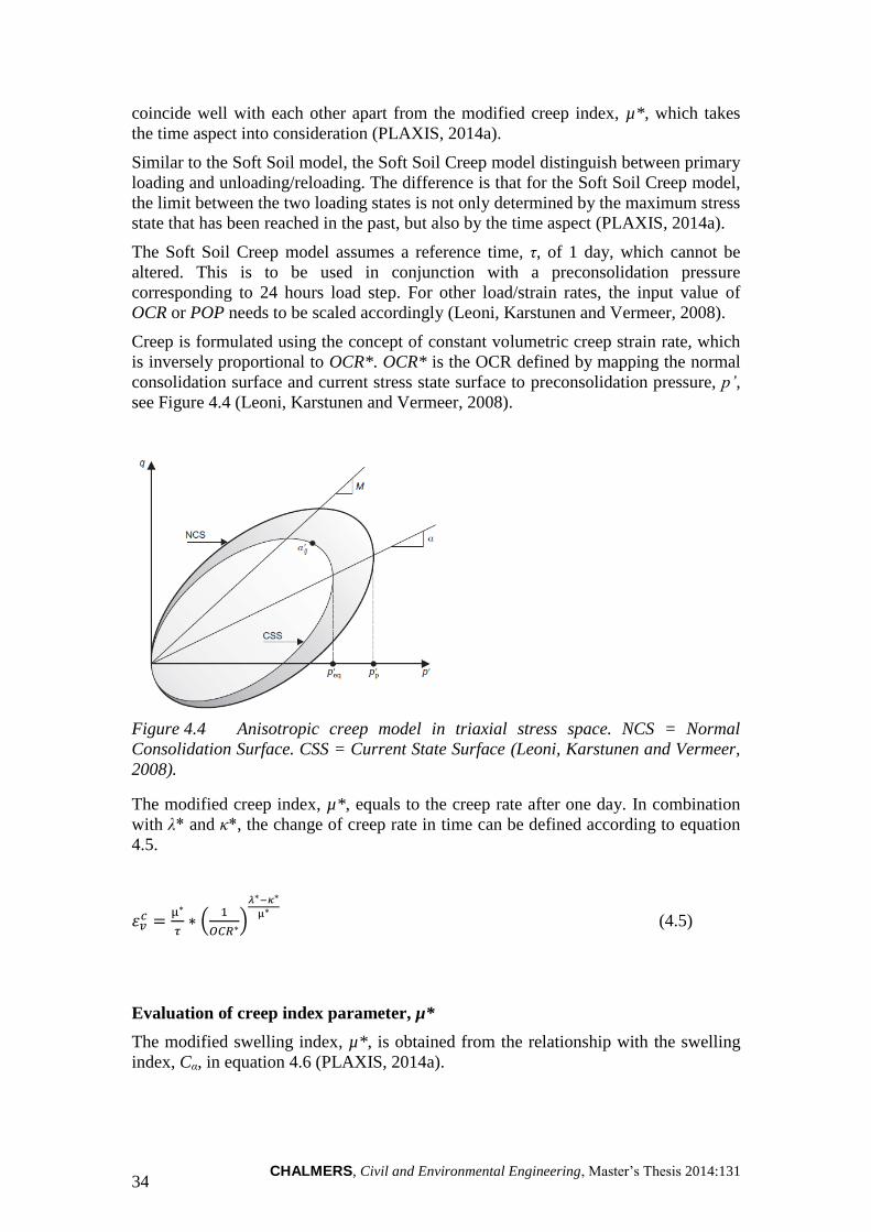
Creep is formulated using the concept of constant volumetric creep strain rate, which
is inversely proportional to OCR*. OCR* is the OCR defined by mapping the normal
consolidation surface and current stress state surface to preconsolidation pressure, p’,
see Figure 4.4 (Leoni, Karstunen and Vermeer, 2008).
Figure 4.4 Anisotropic creep model in triaxial stress space. NCS = Normal
Consolidation Surface. CSS = Current State Surface (Leoni, Karstunen and Vermeer,
2008).
The modified creep index, µ*, equals to the creep rate after one day. In combination
with λ* and κ*, the change of creep rate in time can be defined according to equation
4.5.
(
)
(4.5)
Evaluation of creep index parameter, µ*
The modified swelling index, µ*, is obtained from the relationship with the swelling
index, Cα, in equation 4.6 (PLAXIS, 2014a).
CHALMERS, Civil and Environmental Engineering, Master’s Thesis 2014:131 35
( ) (4.6)
When applying a load step, both consolidation and creep will occur simultaneously.
For a proper parameter evaluation of the creep parameter, µ*, when plotting the strain
versus the natural logarithm of time, the time period needs to be long enough for the
inclination of settlement curve to be straight, i.e. after full consolidation. This makes
the consolidation settlement contribution from µ* minor compared to the contribution
of creep (Waterman and Broere, 2005).
4.3 Structural elements
The structural elements that are used in this thesis are presented below.
Plate element 4.3.1
Plate elements are structural objects used to model slender structures. They are often
suitable to use when simulating the influence of walls or plates. In the plane strain
model the plate extends in the out-of-plane direction.
The plates in the plane strain model have two translational degrees of freedom (ux, uy)
and one rotational degree of freedom (ϕz). The plate elements are based on Mindlin’s
beam theory which allows for deflections due to bending as well as shearing. The
plate element can also change length when axial force is applied. When a prescribed
maximum bending moment or axial force is exceeded the element becomes plastic
(PLAXIS, 2014b).
In order to allow for a proper modeling of soil-structure interaction, an interface can
be applied to a structural element (PLAXIS, 2014b).
Plate element parameters
The general properties are:
deq: Equivalent thickness of the plate. Automatically calculated from
stiffness parameters EA and EI, see Stiffness properties. [m]
wplate: Weight of the plate material per unit of length per unit of width in the
out-of-plane direction [kN/m/m]
The stiffness properties are:
EI: The flexural rigidity, or bending stiffness, for a rectangular cross
section is calculated according to equation 4.8.
CHALMERS, Civil and Environmental Engineering, Master’s Thesis 2014:131 36
(4.8)
EA: The normal stiffness, for a rectangular cross section is calculated
according to equation 4.9.
(4.9)
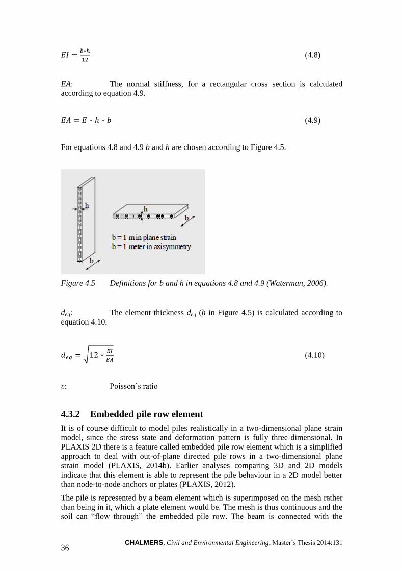
For equations 4.8 and 4.9 b and h are chosen according to Figure 4.5.
Figure 4.5 Definitions for b and h in equations 4.8 and 4.9 (Waterman, 2006).
deq: The element thickness deq (h in Figure 4.5) is calculated according to
equation 4.10.
√
(4.10)
υ: Poisson’s ratio
Embedded pile row element 4.3.2
It is of course difficult to model piles realistically in a two-dimensional plane strain
model, since the stress state and deformation pattern is fully three-dimensional. In
PLAXIS 2D there is a feature called embedded pile row element which is a simplified
approach to deal with out-of-plane directed pile rows in a two-dimensional plane
strain model (PLAXIS, 2014b). Earlier analyses comparing 3D and 2D models
indicate that this element is able to represent the pile behaviour in a 2D model better
than node-to-node anchors or plates (PLAXIS, 2012).
The pile is represented by a beam element which is superimposed on the mesh rather
than being in it, which a plate element would be. The mesh is thus continuous and the
soil can “flow through” the embedded pile row. The beam is connected with the
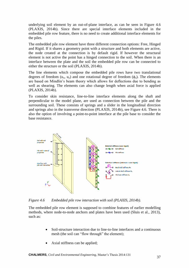
CHALMERS, Civil and Environmental Engineering, Master’s Thesis 2014:131 37
underlying soil element by an out-of-plane interface, as can be seen in Figure 4.6
(PLAXIS, 2014b). Since there are special interface elements included in the
embedded pile row feature, there is no need to create additional interface elements for
the piles.
The embedded pile row element have three different connection options: Free, Hinged
and Rigid. If it shares a geometry point with a structure and both elements are active,
the node created at the connection is by default rigid. If however the structural
element is not active the point has a hinged connection to the soil. When there is an
interface between the plate and the soil the embedded pile row can be connected to
either the structure or the soil (PLAXIS, 2014b).
The line elements which compose the embedded pile rows have two translational
degrees of freedom (ux, uy) and one rotational degree of freedom (ϕz). The elements
are based on Mindlin’s beam theory which allows for deflections due to bending as
well as shearing. The elements can also change length when axial force is applied
(PLAXIS, 2014b).
To consider skin resistance, line-to-line interface elements along the shaft and
perpendicular to the model plane, are used as connection between the pile and the
surrounding soil. These consists of springs and a slider in the longitudinal direction
and springs also in the transverse direction (PLAXIS, 2014b), see Figure 4.6. There is
also the option of involving a point-to-point interface at the pile base to consider the
base resistance.
Figure 4.6 Embedded pile row interaction with soil (PLAXIS, 2014b).
The embedded pile row element is supposed to combine features of earlier modelling
methods, where node-to-node anchors and plates have been used (Sluis et al., 2013),
such as:
Soil-structure interaction due to line-to-line interfaces and a continuous
mesh (the soil can “flow through” the element);
Axial stiffness can be applied;
CHALMERS, Civil and Environmental Engineering, Master’s Thesis 2014:131 38
Bending stiffness can be applied;
Structural forces in piles can be obtained;
Unrealistic shear planes are not introduced.
Embedded pile row element parameters
The embedded pile row feature differs somewhat to most finite element methods since
the bearing capacity (skin friction) is considered to be an input parameter rather than
the result of calculation. The input value of this is preferably based on representative
data from pile load testing. It is advised to compare the behaviour from a calibration
with the results from the pile load test. The group action of the pile row must be taken
into account when defining the pile bearing capacity (PLAXIS, 2014b).
The single pile material properties:
E: Young’s modulus. [kN/m2]
γpile: Unit weight of pile material. [kN/m3]
The geometric properties of the embedded pile row:
Pile type: Predefined or User defined can be chosen
Predefined pile type: Massive circular pile, Circular tube or Massive square pile can
be chosen.
dpile: For Massive circular pile, the pile diameter is defined
and determines the size of the elastic zone where soil behaviour is excluded. [m]
User-defined piles are defined by the pile cross section area, A, and moment of inertia,
I.
Lspacing: Pile spacing perpendicular to the model plane. [m]
The interaction properties of the embedded pile row:
In order to describe the behaviour of the special interface element, an elastic-plastic
model is used. The elastic behaviour accounts for the difference in average soil
displacements and the displacements of piles in the out-of-plane direction and
depends on the pile diameter in relation to Lspacing. The plastic behaviour is regarded
CHALMERS, Civil and Environmental Engineering, Master’s Thesis 2014:131 39
by skin resistance Tmax [kN/m], defined at the pile top and bottom, Ttop,max and Tbot,max,
and Base resistance [kN]. These values are automatically recalculated per unit of
width in the out-of-plane direction (PLAXIS, 2014b).
For the interface to remain elastic the shear force t.s must be lower than Tmax. When it
is exceeded the behaviour is plastic. The pile bearing capacities are automatically
recalculated per unit of width in the out-of-plane direction by using the Lspacing input
(PLAXIS, 2014b).
4.4 Loads in PLAXIS 2D
A point load are created in a similar manner as geometry points and given the input
value in force per unit of width [kN/m] in the direction perpendicular to the model
plane. In the 2D plane strain model the point load thus is a line load. Also in the
axisymmetric model the point load is a line load, in this case on a circle section, if not
located at x = 0, where it is a real point load and the input value is given in the unit of
force [kN] (PLAXIS, 2014b).
Distributed loads are created in a similar manner as geometry lines. Like the point
load, the distributed load extends in the out-of-plane direction and thus has the input
value of force per area [kN/m2]. In the input window for distributed loads the input
values for the two geometry points at each end of the load line can be applied. The
load can be uniform if the same value is given to the two points. If there is a
difference between the input values the load is linear along the line (PLAXIS, 2014b).
Characteristic values of the loads are used as input for PLAXIS.

CHALMERS, Civil and Environmental Engineering, Master’s Thesis 2014:131 40
5 Verification of soil parameters and soil models
This chapter contains information about how evaluated parameters have been adjusted
to give an accurate representation of the soil in the PLAXIS 2D model.
5.1 Soil tests performed in PLAXIS 2D
An important aspect of creating models using numerical software is to be able to
validate that the model is acting as anticipated. In order to verify that the soil model
created in PLAXIS is able to express the actual behaviour of the in situ soil, it is
possible to simulate different kinds of soil tests in PLAXIS. Soil test results from real
laboratory tests can be compared with the results from simulated tests in PLAXIS and
thus show if the model corresponds to the real case in a realistic way. Based on the
comparison, the input parameters could be calibrated to find the optimal input values.
For this thesis the stepwise oedometer tests carried out in 1966, used to evaluate the
soil parameters, have been simulated using an axisymmetric model as described
below. To compare the shear strength, triaxial test simulations have also been carried
out.
The oedometer tests from 1966 were not fully performed according to the
recommended practice, with the time for each loading step set to one day. Several
load steps have been applied for shorter periods. This has been taken into account in
the soil test simulations by using the same length of time steps, as in the oedometer
tests from 1966.
As is described in section 6.1, the clay below the excavation bottom is in this thesis
divided into three different layers. Soil tests simulations, both oedometer and triaxial,
with the Soft Soil model have been performed for each of the three layers. The Soft
Soil Creep model has only been evaluated with an oedometer simulation and only for
Clay 1. The Soft Soil Creep simulation is made as a comparison with the Soft Soil
model. Therefore, the curve of the Soft Soil Creep has not been modified.
Axisymmetric model, Stepwise oedometer test 5.1.1
A stepwise oedometer test is simulated in PLAXIS as an axisymmetric scale model
with a closed consolidation boundary and dimensions according to Figure 5.1. When
performing the soil test simulations by scale modelling rather than the Soil Test
feature in PLAXIS 2D, the possibility to set time is given. This should be the
preferred way to model, especially for Soft Soil Creep which is time dependent.
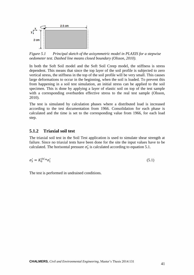
CHALMERS, Civil and Environmental Engineering, Master’s Thesis 2014:131 41
Figure 5.1 Principal sketch of the axisymmetric model in PLAXIS for a stepwise
oedometer test. Dashed line means closed boundary (Olsson, 2010).
In both the Soft Soil model and the Soft Soil Creep model, the stiffness is stress
dependent. This means that since the top layer of the soil profile is subjected to zero
vertical stress, the stiffness in the top of the soil profile will be very small. This causes
large deformations to occur in the beginning, when the soil is loaded. To prevent this
from happening in a soil test simulation, an initial stress can be applied to the soil
specimen. This is done by applying a layer of elastic soil on top of the test sample
with a corresponding overburden effective stress to the real test sample (Olsson,
2010).
The test is simulated by calculation phases where a distributed load is increased
according to the test documentation from 1966. Consolidation for each phase is
calculated and the time is set to the corresponding value from 1966, for each load
step.
Triaxial soil test 5.1.2
The triaxial soil test in the Soil Test application is used to simulate shear strength at
failure. Since no triaxial tests have been done for the site the input values have to be
calculated. The horisontal pressure is calculated according to equation 5.1.
* (5.1)
The test is performed in undrained conditions.
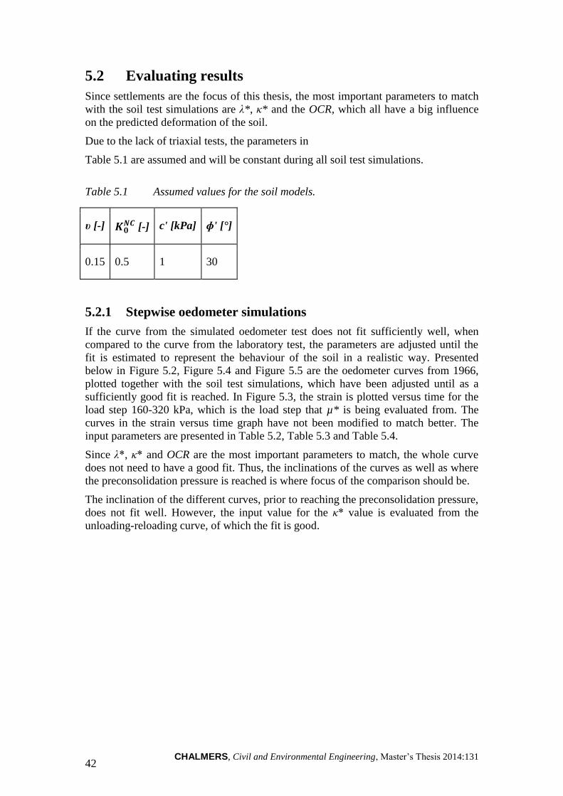
CHALMERS, Civil and Environmental Engineering, Master’s Thesis 2014:131 42
5.2 Evaluating results
Since settlements are the focus of this thesis, the most important parameters to match
with the soil test simulations are λ*, κ* and the OCR, which all have a big influence
on the predicted deformation of the soil.
Due to the lack of triaxial tests, the parameters in
Table 5.1 are assumed and will be constant during all soil test simulations.
Table 5.1 Assumed values for the soil models.
υ [-] [-] c' [kPa] ɸ' [°]
0.15 0.5 1 30
Stepwise oedometer simulations 5.2.1
If the curve from the simulated oedometer test does not fit sufficiently well, when
compared to the curve from the laboratory test, the parameters are adjusted until the
fit is estimated to represent the behaviour of the soil in a realistic way. Presented
below in Figure 5.2, Figure 5.4 and Figure 5.5 are the oedometer curves from 1966,
plotted together with the soil test simulations, which have been adjusted until as a
sufficiently good fit is reached. In Figure 5.3, the strain is plotted versus time for the
load step 160-320 kPa, which is the load step that µ* is being evaluated from. The
curves in the strain versus time graph have not been modified to match better. The
input parameters are presented in Table 5.2, Table 5.3 and Table 5.4.
Since λ*, κ* and OCR are the most important parameters to match, the whole curve
does not need to have a good fit. Thus, the inclinations of the curves as well as where
the preconsolidation pressure is reached is where focus of the comparison should be.
The inclination of the different curves, prior to reaching the preconsolidation pressure,
does not fit well. However, the input value for the κ* value is evaluated from the
unloading-reloading curve, of which the fit is good.
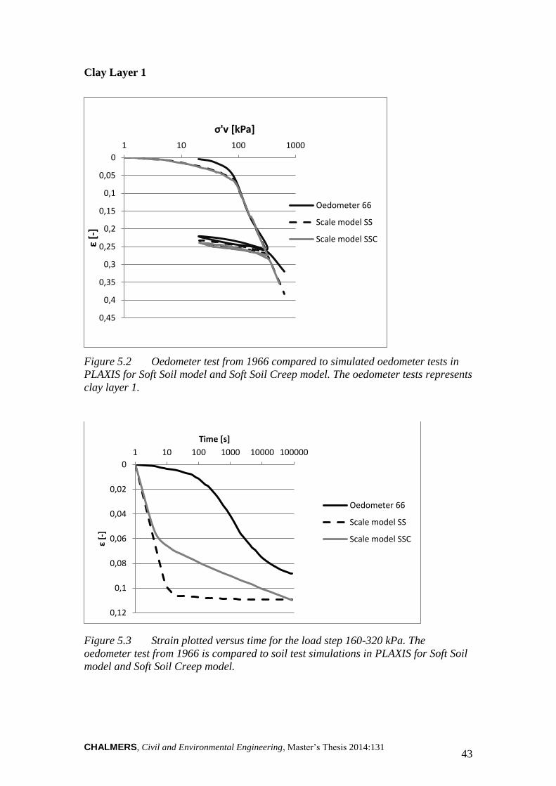
CHALMERS, Civil and Environmental Engineering, Master’s Thesis 2014:131 43
Clay Layer 1
Figure 5.2 Oedometer test from 1966 compared to simulated oedometer tests in
PLAXIS for Soft Soil model and Soft Soil Creep model. The oedometer tests represents
clay layer 1.
Figure 5.3 Strain plotted versus time for the load step 160-320 kPa. The
oedometer test from 1966 is compared to soil test simulations in PLAXIS for Soft Soil
model and Soft Soil Creep model.
0
0,05
0,1
0,15
0,2
0,25
0,3
0,35
0,4
0,45
1 10 100 1000
ε [-
]
σ'v [kPa]
Oedometer 66
Scale model SS
Scale model SSC
0
0,02
0,04
0,06
0,08
0,1
0,12
1 10 100 1000 10000 100000
ε [-
]
Time [s]
Oedometer 66
Scale model SS
Scale model SSC
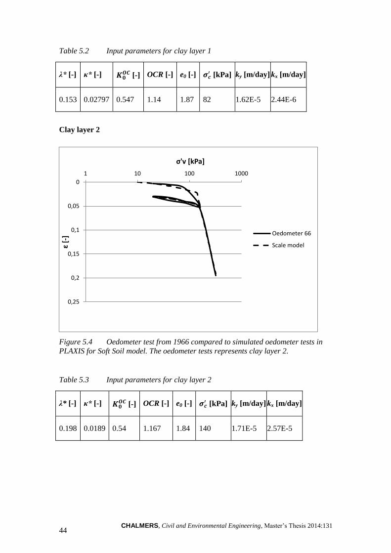
CHALMERS, Civil and Environmental Engineering, Master’s Thesis 2014:131 44
Table 5.2 Input parameters for clay layer 1
λ* [-] κ* [-] [-] OCR [-] e0 [-]
[kPa] ky [m/day] kx [m/day]
0.153 0.02797 0.547 1.14 1.87 82 1.62E-5 2.44E-6
Clay layer 2
Figure 5.4 Oedometer test from 1966 compared to simulated oedometer tests in
PLAXIS for Soft Soil model. The oedometer tests represents clay layer 2.
Table 5.3 Input parameters for clay layer 2
λ* [-] κ* [-] [-] OCR [-] e0 [-]
[kPa] ky [m/day] kx [m/day]
0.198 0.0189 0.54 1.167 1.84 140 1.71E-5 2.57E-5
0
0,05
0,1
0,15
0,2
0,25
1 10 100 1000
ε [-
]
σ'v [kPa]
Oedometer 66
Scale model
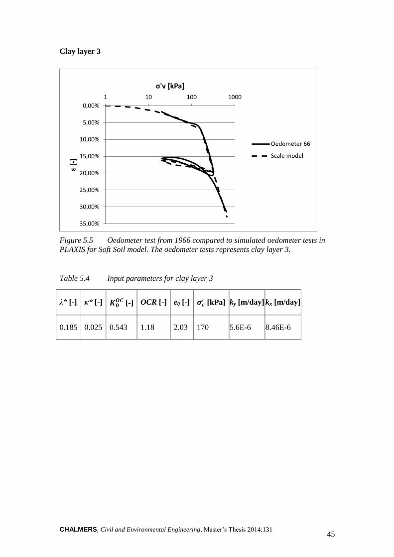
CHALMERS, Civil and Environmental Engineering, Master’s Thesis 2014:131 45
Clay layer 3
Figure 5.5 Oedometer test from 1966 compared to simulated oedometer tests in
PLAXIS for Soft Soil model. The oedometer tests represents clay layer 3.
Table 5.4 Input parameters for clay layer 3
λ* [-] κ* [-] [-] OCR [-] e0 [-]
[kPa] ky [m/day] kx [m/day]
0.185 0.025 0.543 1.18 2.03 170 5.6E-6 8.46E-6
0,00%
5,00%
10,00%
15,00%
20,00%
25,00%
30,00%
35,00%
1 10 100 1000
ε [-
]
σ'v [kPa]
Oedometer 66
Scale model
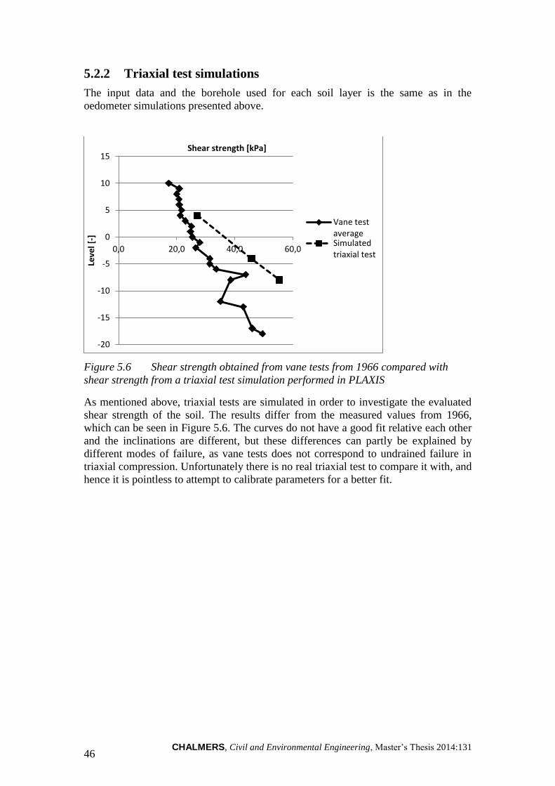
CHALMERS, Civil and Environmental Engineering, Master’s Thesis 2014:131 46
Triaxial test simulations 5.2.2
The input data and the borehole used for each soil layer is the same as in the
oedometer simulations presented above.
Figure 5.6 Shear strength obtained from vane tests from 1966 compared with
shear strength from a triaxial test simulation performed in PLAXIS
As mentioned above, triaxial tests are simulated in order to investigate the evaluated
shear strength of the soil. The results differ from the measured values from 1966,
which can be seen in Figure 5.6. The curves do not have a good fit relative each other
and the inclinations are different, but these differences can partly be explained by
different modes of failure, as vane tests does not correspond to undrained failure in
triaxial compression. Unfortunately there is no real triaxial test to compare it with, and
hence it is pointless to attempt to calibrate parameters for a better fit.
-20
-15
-10
-5
0
5
10
15
0,0 20,0 40,0 60,0
Leve
l [-]
Shear strength [kPa]
Vane testaverageSimulatedtriaxial test
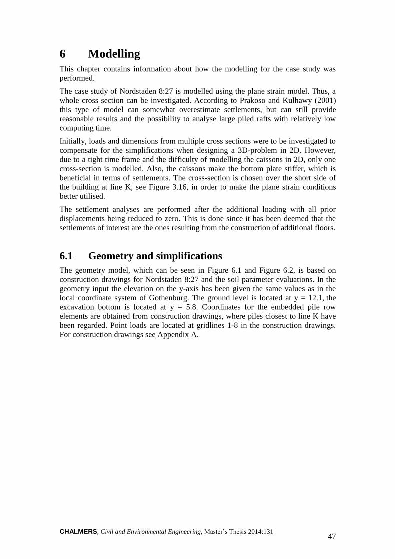
CHALMERS, Civil and Environmental Engineering, Master’s Thesis 2014:131 47
6 Modelling
This chapter contains information about how the modelling for the case study was
performed.
The case study of Nordstaden 8:27 is modelled using the plane strain model. Thus, a
whole cross section can be investigated. According to Prakoso and Kulhawy (2001)
this type of model can somewhat overestimate settlements, but can still provide
reasonable results and the possibility to analyse large piled rafts with relatively low
computing time.
Initially, loads and dimensions from multiple cross sections were to be investigated to
compensate for the simplifications when designing a 3D-problem in 2D. However,
due to a tight time frame and the difficulty of modelling the caissons in 2D, only one
cross-section is modelled. Also, the caissons make the bottom plate stiffer, which is
beneficial in terms of settlements. The cross-section is chosen over the short side of
the building at line K, see Figure 3.16, in order to make the plane strain conditions
better utilised.
The settlement analyses are performed after the additional loading with all prior
displacements being reduced to zero. This is done since it has been deemed that the
settlements of interest are the ones resulting from the construction of additional floors.
6.1 Geometry and simplifications
The geometry model, which can be seen in Figure 6.1 and Figure 6.2, is based on
construction drawings for Nordstaden 8:27 and the soil parameter evaluations. In the
geometry input the elevation on the y-axis has been given the same values as in the
local coordinate system of Gothenburg. The ground level is located at y = 12.1, the
excavation bottom is located at y = 5.8. Coordinates for the embedded pile row
elements are obtained from construction drawings, where piles closest to line K have
been regarded. Point loads are located at gridlines 1-8 in the construction drawings.
For construction drawings see Appendix A.
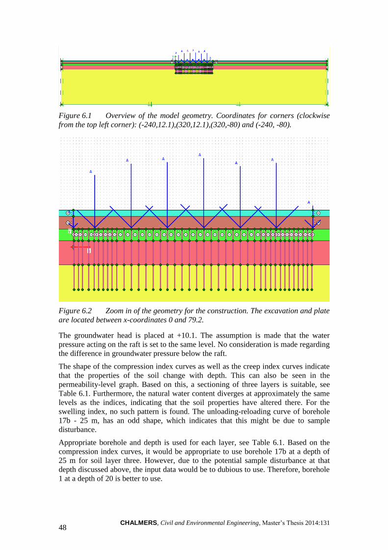
CHALMERS, Civil and Environmental Engineering, Master’s Thesis 2014:131 48
Figure 6.1 Overview of the model geometry. Coordinates for corners (clockwise
from the top left corner): (-240,12.1),(320,12.1),(320,-80) and (-240, -80).
Figure 6.2 Zoom in of the geometry for the construction. The excavation and plate
are located between x-coordinates 0 and 79.2.
The groundwater head is placed at +10.1. The assumption is made that the water
pressure acting on the raft is set to the same level. No consideration is made regarding
the difference in groundwater pressure below the raft.
The shape of the compression index curves as well as the creep index curves indicate
that the properties of the soil change with depth. This can also be seen in the
permeability-level graph. Based on this, a sectioning of three layers is suitable, see
Table 6.1. Furthermore, the natural water content diverges at approximately the same
levels as the indices, indicating that the soil properties have altered there. For the
swelling index, no such pattern is found. The unloading-reloading curve of borehole
17b - 25 m, has an odd shape, which indicates that this might be due to sample
disturbance.
Appropriate borehole and depth is used for each layer, see Table 6.1. Based on the
compression index curves, it would be appropriate to use borehole 17b at a depth of
25 m for soil layer three. However, due to the potential sample disturbance at that
depth discussed above, the input data would be to dubious to use. Therefore, borehole
1 at a depth of 20 is better to use.

CHALMERS, Civil and Environmental Engineering, Master’s Thesis 2014:131 49
Table 6.1 Levels for the layers modelled as Linear Elastic (LE) and Soft Soil and
sample used for the corresponding input parameters for the Soft Soil layers.
Start level, y End level, y Borehole and depth
LE layer 1 (fill) +12.1 +10.1 -
LE layer 2 +10.1 +5.8 -
Clay layer 1 +5.8 +2 Borehole 1, 8m
Clay layer 2 +2 -6 Borehole 17b, 16m
Clay layer 3 -6 -90 Borehole 1, 20 m
The stress-void ratio curves, evaluated from the soil tests, in Figure 6.3, show two
distinct trends. This might imply that there would be sufficient with two layers for the
model. However, only the compression indices for the chosen two deeper layers are
similar. The rest of the parameters differ too much to model it as one layer.
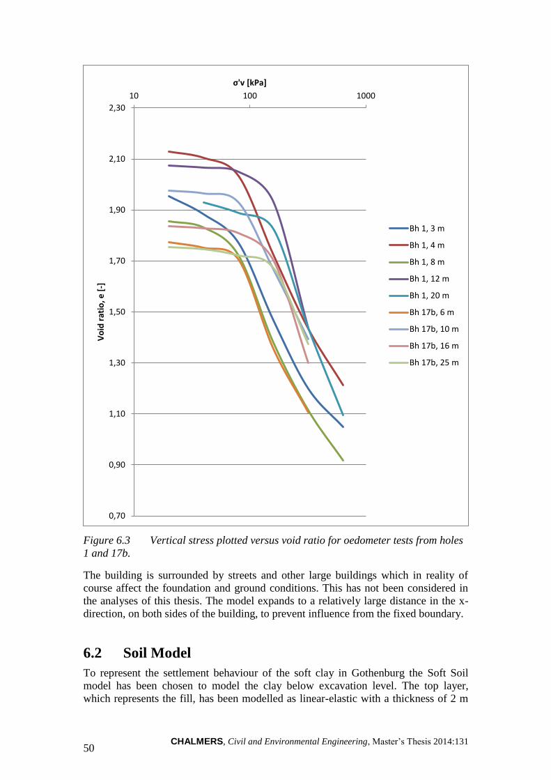
CHALMERS, Civil and Environmental Engineering, Master’s Thesis 2014:131 50
Figure 6.3 Vertical stress plotted versus void ratio for oedometer tests from holes
1 and 17b.
The building is surrounded by streets and other large buildings which in reality of
course affect the foundation and ground conditions. This has not been considered in
the analyses of this thesis. The model expands to a relatively large distance in the x-
direction, on both sides of the building, to prevent influence from the fixed boundary.
6.2 Soil Model
To represent the settlement behaviour of the soft clay in Gothenburg the Soft Soil
model has been chosen to model the clay below excavation level. The top layer,
which represents the fill, has been modelled as linear-elastic with a thickness of 2 m
0,70
0,90
1,10
1,30
1,50
1,70
1,90
2,10
2,30
10 100 1000V
oid
rat
io, e
[-]
σ'v [kPa]
Bh 1, 3 m
Bh 1, 4 m
Bh 1, 8 m
Bh 1, 12 m
Bh 1, 20 m
Bh 17b, 6 m
Bh 17b, 10 m
Bh 17b, 16 m
Bh 17b, 25 m
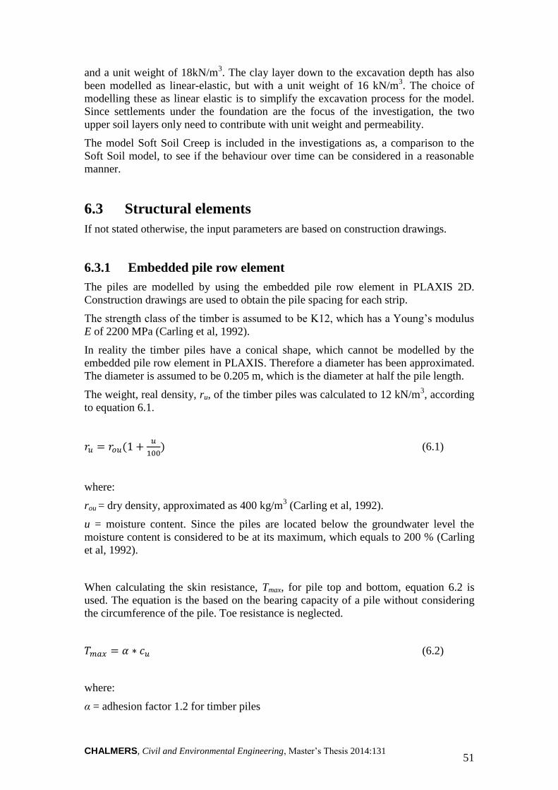
CHALMERS, Civil and Environmental Engineering, Master’s Thesis 2014:131 51
and a unit weight of 18kN/m3. The clay layer down to the excavation depth has also
been modelled as linear-elastic, but with a unit weight of 16 kN/m3. The choice of
modelling these as linear elastic is to simplify the excavation process for the model.
Since settlements under the foundation are the focus of the investigation, the two
upper soil layers only need to contribute with unit weight and permeability.
The model Soft Soil Creep is included in the investigations as, a comparison to the
Soft Soil model, to see if the behaviour over time can be considered in a reasonable
manner.
6.3 Structural elements
If not stated otherwise, the input parameters are based on construction drawings.
Embedded pile row element 6.3.1
The piles are modelled by using the embedded pile row element in PLAXIS 2D.
Construction drawings are used to obtain the pile spacing for each strip.
The strength class of the timber is assumed to be K12, which has a Young’s modulus
E of 2200 MPa (Carling et al, 1992).
In reality the timber piles have a conical shape, which cannot be modelled by the
embedded pile row element in PLAXIS. Therefore a diameter has been approximated.
The diameter is assumed to be 0.205 m, which is the diameter at half the pile length.
The weight, real density, ru, of the timber piles was calculated to 12 kN/m3, according
to equation 6.1.
(
) (6.1)
where:
rou = dry density, approximated as 400 kg/m3 (Carling et al, 1992).
u = moisture content. Since the piles are located below the groundwater level the
moisture content is considered to be at its maximum, which equals to 200 % (Carling
et al, 1992).
When calculating the skin resistance, Tmax, for pile top and bottom, equation 6.2 is
used. The equation is the based on the bearing capacity of a pile without considering
the circumference of the pile. Toe resistance is neglected.
(6.2)
where:
α = adhesion factor 1.2 for timber piles
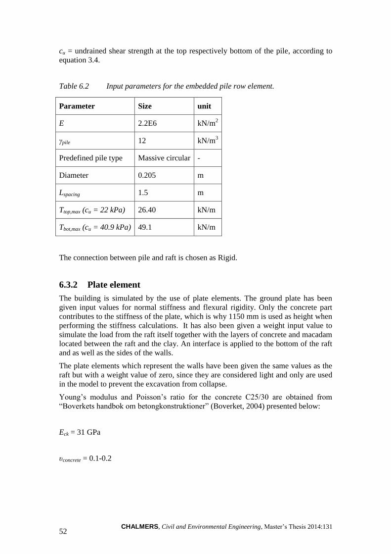
CHALMERS, Civil and Environmental Engineering, Master’s Thesis 2014:131 52
cu = undrained shear strength at the top respectively bottom of the pile, according to
equation 3.4.
Table 6.2 Input parameters for the embedded pile row element.
Parameter Size unit
E 2.2E6 kN/m2
γpile 12 kN/m3
Predefined pile type Massive circular -
Diameter 0.205 m
Lspacing 1.5 m
Ttop,max (cu = 22 kPa) 26.40 kN/m
Tbot,max (cu = 40.9 kPa) 49.1 kN/m
The connection between pile and raft is chosen as Rigid.
Plate element 6.3.2
The building is simulated by the use of plate elements. The ground plate has been
given input values for normal stiffness and flexural rigidity. Only the concrete part
contributes to the stiffness of the plate, which is why 1150 mm is used as height when
performing the stiffness calculations. It has also been given a weight input value to
simulate the load from the raft itself together with the layers of concrete and macadam
located between the raft and the clay. An interface is applied to the bottom of the raft
and as well as the sides of the walls.
The plate elements which represent the walls have been given the same values as the
raft but with a weight value of zero, since they are considered light and only are used
in the model to prevent the excavation from collapse.
Young’s modulus and Poisson’s ratio for the concrete C25/30 are obtained from
“Boverkets handbok om betongkonstruktioner” (Boverket, 2004) presented below:
Eck = 31 GPa
υconcrete = 0.1-0.2
CHALMERS, Civil and Environmental Engineering, Master’s Thesis 2014:131 53
For long-term loads5, Young’s modulus is approximated as 0.5 * Eck.
The input parameters for slab and walls are presented in Table 6.3.
Table 6.3 Input parameters for the plate elements.
Slab Walls [unit]
EA1 17.83E9 17.83E9 kN/m
EI 1.964E9 1.964E9 kNm2/m
w 39.80 0 kN/m/m
υconcrete 0.2 0.2 -
6.4 Loads
To consider the loads from the building, load elements and properties assigned to
structural elements have been used when modelling. Each structural element is
assigned with its corresponding weight.
The remaining load from the structure above the plate is modelled by point load
elements, where the pillars are placed. The loads from the pillars are entered as point
loads in PLAXIS, but since the model is in 2D, the input unit is kN/m. Thus an
approximation is made. A point load is divided by the in plane width between two
pillars, in order to get an average load per meter. The distribution of the loads between
the pillars is based on the theory of continuous beams with uniformly distributed
loads, according to Appendix D.
Load scenarios 6.4.1
In order to simulate different scenarios describing how many floors are added to the
building, five loading scenarios, 10 kPa–50 kPa, have been chosen, with the
assumption that each new floor increases the load with 10 kPa. Since the original
weight of the building is fully compensated by the excavation of soil (104.8 - 96 = 8.8
kPa), the net increment of each load step is 8.8 kPa less than stated.
10 kPa: +10 kPa in total stress = +1.2 kPa in effective stress
20 kPa: +20 kPa in total stress = +11.2 kPa in effective stress
30 kPa: +30 kPa in total stress = +21.2 kPa in effective stress
40 kPa: +40 kPa in total stress = +31.2 kPa in effective stress
50 kPa: +50 kPa in total stress = +41.2 kPa in effective stress
This increment is equally distributed to the point loads by multiplying each point load
with a corresponding factor, see Appendix C.
5 Hans Lindewald, Structural Engineer at ELU, interviewed 14-03-17
CHALMERS, Civil and Environmental Engineering, Master’s Thesis 2014:131 54
6.5 Mesh optimization
A medium coarseness of the grid has been chosen. A finer mesh was tested but the
differences were deemed to be negligible.
6.6 Phases
The different phases are presented below:
1. Initial phase
Represents the ground conditions before the construction of the building begins. A
phreatic level of y = 10.1 is chosen.
2. Piles
The embedded pile row elements are activated. Undrained behaviour is ignored and
displacement are reset to zero.
3. Construction (drained)
The excavation and construction are simulated as an instantaneous event by
deactivating the soil clusters and activating the plate elements and loads. No time
aspect is given to the construction to prevent the sides of the excavation from
collapsing. Undrained behaviour is ignored and replacements are reset to zero.
4. Construction of x number of additional floors (undrained)
Every point load is increased by a factor which corresponds to the total load
increment, depending on which loading scenario that is being tested. No time aspect
of the construction is taken into consideration.
5. Consolidation
A consolidation analysis for the first 10 years is performed.
6. Consolidation
A consolidation analysis for the first 40 years is performed.
7. Consolidation (90%)
A consolidation analysis until 90% of the excess pore water pressure has dissipated is
performed.
To create the current conditions in the model, the time span until today was simulated
in drained conditions. This assumption is based on the settlement readings, which
indicates that there is close to none consolidation occurring today. Also, it is difficult
to model the conditions of today in a realistic way. Since the building is more than
fully compensated, a simulation in PLAXIS will cause the soil to heave. The
settlement readings indicates that some parts do heave, but there has also been
settlement occurring. The assumption of using drained scenario results in a state
where there are no excess pore water pressures in the ground at the time additional
loads are applied.
A model with undrained conditions, for phase 3 (“3. Construction”), with a following
consolidation phase until today, 40 years, will also be simulated. This is done both to
compare the current settlement readings with the results from the PLAXIS model as
well as to analyse what effects the assumption of a drained scenario in phase 3 has.
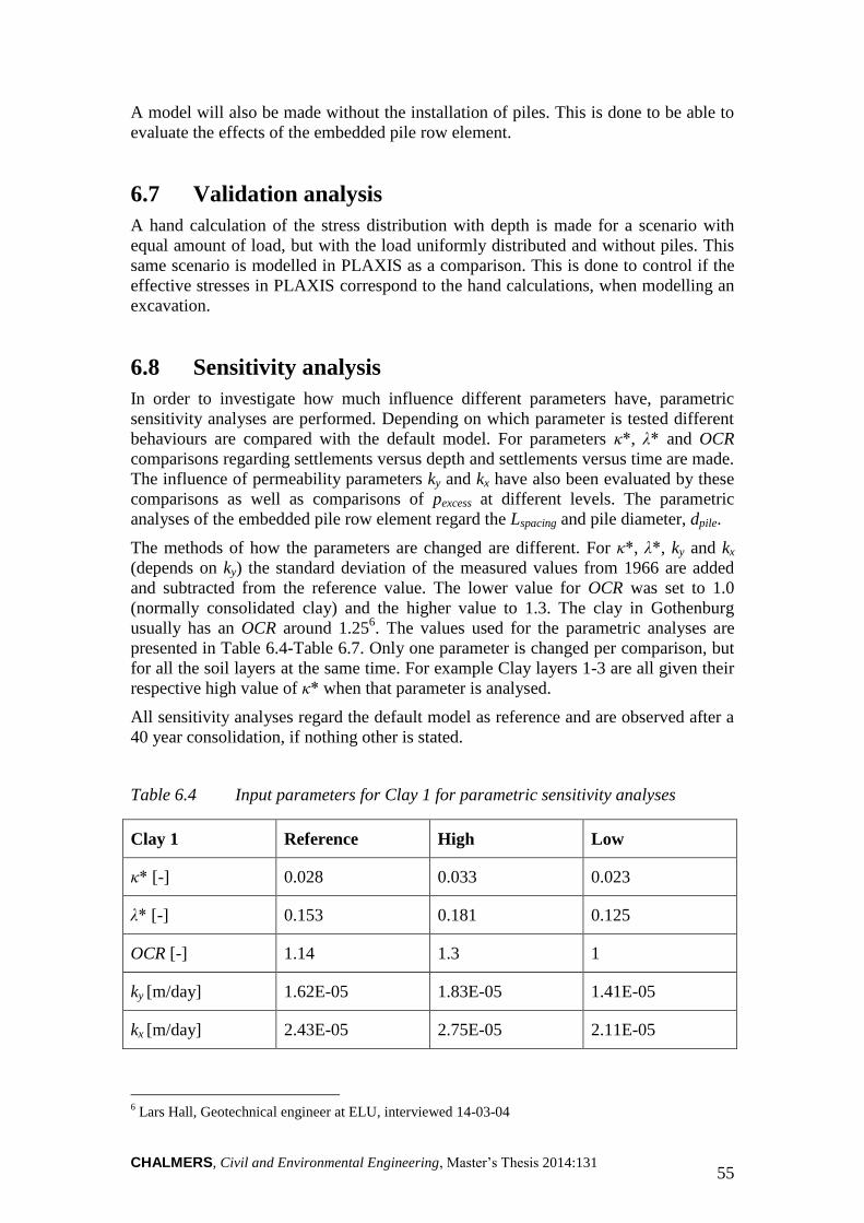
CHALMERS, Civil and Environmental Engineering, Master’s Thesis 2014:131 55
A model will also be made without the installation of piles. This is done to be able to
evaluate the effects of the embedded pile row element.
6.7 Validation analysis
A hand calculation of the stress distribution with depth is made for a scenario with
equal amount of load, but with the load uniformly distributed and without piles. This
same scenario is modelled in PLAXIS as a comparison. This is done to control if the
effective stresses in PLAXIS correspond to the hand calculations, when modelling an
excavation.
6.8 Sensitivity analysis
In order to investigate how much influence different parameters have, parametric
sensitivity analyses are performed. Depending on which parameter is tested different
behaviours are compared with the default model. For parameters κ*, λ* and OCR
comparisons regarding settlements versus depth and settlements versus time are made.
The influence of permeability parameters ky and kx have also been evaluated by these
comparisons as well as comparisons of pexcess at different levels. The parametric
analyses of the embedded pile row element regard the Lspacing and pile diameter, dpile.
The methods of how the parameters are changed are different. For κ*, λ*, ky and kx
(depends on ky) the standard deviation of the measured values from 1966 are added
and subtracted from the reference value. The lower value for OCR was set to 1.0
(normally consolidated clay) and the higher value to 1.3. The clay in Gothenburg
usually has an OCR around 1.256. The values used for the parametric analyses are
presented in Table 6.4-Table 6.7. Only one parameter is changed per comparison, but
for all the soil layers at the same time. For example Clay layers 1-3 are all given their
respective high value of κ* when that parameter is analysed.
All sensitivity analyses regard the default model as reference and are observed after a
40 year consolidation, if nothing other is stated.
Table 6.4 Input parameters for Clay 1 for parametric sensitivity analyses
Clay 1 Reference High Low
κ* [-] 0.028 0.033 0.023
λ* [-] 0.153 0.181 0.125
OCR [-] 1.14 1.3 1
ky [m/day] 1.62E-05 1.83E-05 1.41E-05
kx [m/day] 2.43E-05 2.75E-05 2.11E-05
6 Lars Hall, Geotechnical engineer at ELU, interviewed 14-03-04
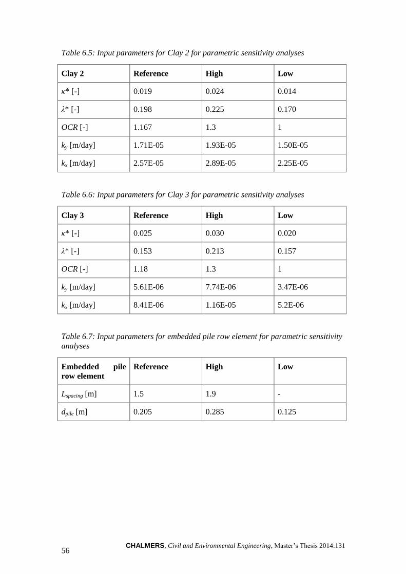
CHALMERS, Civil and Environmental Engineering, Master’s Thesis 2014:131 56
Table 6.5: Input parameters for Clay 2 for parametric sensitivity analyses
Clay 2 Reference High Low
κ* [-] 0.019 0.024 0.014
λ* [-] 0.198 0.225 0.170
OCR [-] 1.167 1.3 1
ky [m/day] 1.71E-05 1.93E-05 1.50E-05
kx [m/day] 2.57E-05 2.89E-05 2.25E-05
Table 6.6: Input parameters for Clay 3 for parametric sensitivity analyses
Clay 3 Reference High Low
κ* [-] 0.025 0.030 0.020
λ* [-] 0.153 0.213 0.157
OCR [-] 1.18 1.3 1
ky [m/day] 5.61E-06 7.74E-06 3.47E-06
kx [m/day] 8.41E-06 1.16E-05 5.2E-06
Table 6.7: Input parameters for embedded pile row element for parametric sensitivity
analyses
Embedded pile
row element
Reference High Low
Lspacing [m] 1.5 1.9 -
dpile [m] 0.205 0.285 0.125

CHALMERS, Civil and Environmental Engineering, Master’s Thesis 2014:131 57
7 Results
Results from the PLAXIS 2D modelling and the hand calculations are presented in
this chapter. Due to the extension of the result chapter, presented in several graphs,
discussion regarding the results has been included in this chapter rather than in a
separate one. This is done in order to make it easier for the reader to comprehend the
discussion.
7.1 Results from PLAXIS analyses
The presented results from the PLAXIS 2D calculations describe the behaviour of the
ground and foundation in form of excess pore water behaviour, pile interaction and
settlements. Relevant loading scenarios and modelling approaches are presented for
each specific comparison. Results from the parametric studies are also presented.
To be able to make comparisons between different models, phases and load scenarios,
a default scenario is chosen. This scenario is labelled as “Piled raft” and has been
chosen according to the following criteria:
The foundation is a piled raft.
The additional load is 20 kPa.
The timespan until today, the first 40 years, has been modelled as a drained
scenario.
Soft Soil is used as soil model.
These criteria apply for “Piled raft” if nothing else is stated. This is also chosen as
“Reference” for the parametric studies.
Note that when it is stated that the data is obtained after a consolidation of 40 years,
this refers to the consolidation after the additional load of 10-50 kPa has been applied.
This should not be confused with the different modelling approaches where the piled
raft either has a drained scenario or a 40 year long consolidation (labelled as “Piled
raft B”) before the additional load is applied. The scenario “Raft only” has the same
criteria as “Piled raft” but with the exception that it considers a raft without piles.
Different load scenarios are presented according to definitions given in section 6.4.1.
Comparisons of the PLAXIS models Soft Soil and Soft Soil Creep are presented as SS
and SSC, respectively.
Combinations of different aspects occur. For example “SSC – 50 kPa” labels a
scenario where the soil model used is Soft Soil Creep and the additional loading is 50
kPa.
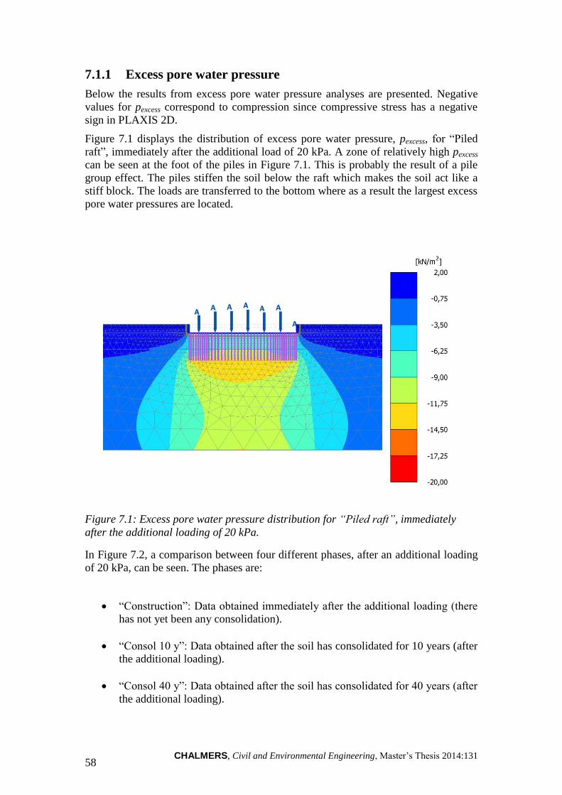
CHALMERS, Civil and Environmental Engineering, Master’s Thesis 2014:131 58
Excess pore water pressure 7.1.1
Below the results from excess pore water pressure analyses are presented. Negative
values for pexcess correspond to compression since compressive stress has a negative
sign in PLAXIS 2D.
Figure 7.1 displays the distribution of excess pore water pressure, pexcess, for “Piled
raft”, immediately after the additional load of 20 kPa. A zone of relatively high pexcess
can be seen at the foot of the piles in Figure 7.1. This is probably the result of a pile
group effect. The piles stiffen the soil below the raft which makes the soil act like a
stiff block. The loads are transferred to the bottom where as a result the largest excess
pore water pressures are located.
Figure 7.1: Excess pore water pressure distribution for “Piled raft”, immediately
after the additional loading of 20 kPa.
In Figure 7.2, a comparison between four different phases, after an additional loading
of 20 kPa, can be seen. The phases are:
“Construction”: Data obtained immediately after the additional loading (there
has not yet been any consolidation).
“Consol 10 y”: Data obtained after the soil has consolidated for 10 years (after
the additional loading).
“Consol 40 y”: Data obtained after the soil has consolidated for 40 years (after
the additional loading).
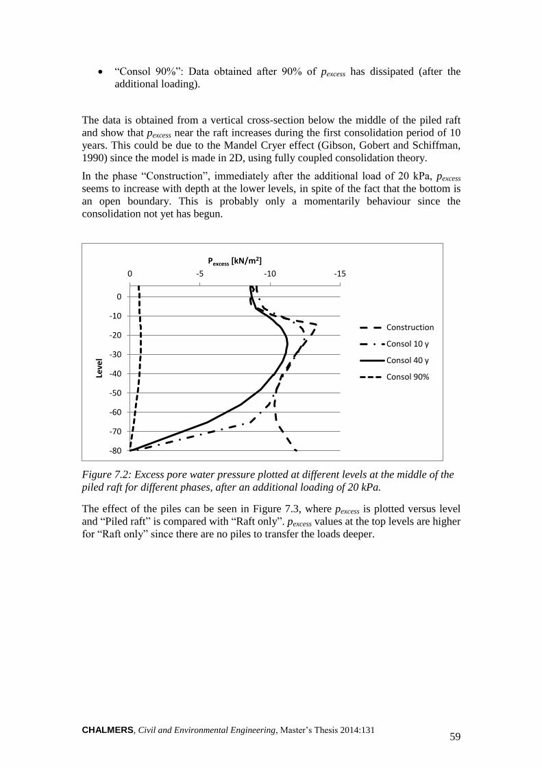
CHALMERS, Civil and Environmental Engineering, Master’s Thesis 2014:131 59
“Consol 90%”: Data obtained after 90% of pexcess has dissipated (after the
additional loading).
The data is obtained from a vertical cross-section below the middle of the piled raft
and show that pexcess near the raft increases during the first consolidation period of 10
years. This could be due to the Mandel Cryer effect (Gibson, Gobert and Schiffman,
1990) since the model is made in 2D, using fully coupled consolidation theory.
In the phase “Construction”, immediately after the additional load of 20 kPa, pexcess
seems to increase with depth at the lower levels, in spite of the fact that the bottom is
an open boundary. This is probably only a momentarily behaviour since the
consolidation not yet has begun.
Figure 7.2: Excess pore water pressure plotted at different levels at the middle of the
piled raft for different phases, after an additional loading of 20 kPa.
The effect of the piles can be seen in Figure 7.3, where pexcess is plotted versus level
and “Piled raft” is compared with “Raft only”. pexcess values at the top levels are higher
for “Raft only” since there are no piles to transfer the loads deeper.
-80
-70
-60
-50
-40
-30
-20
-10
0
-15-10-50
Leve
l
Pexcess [kN/m2]
Construction
Consol 10 y
Consol 40 y
Consol 90%
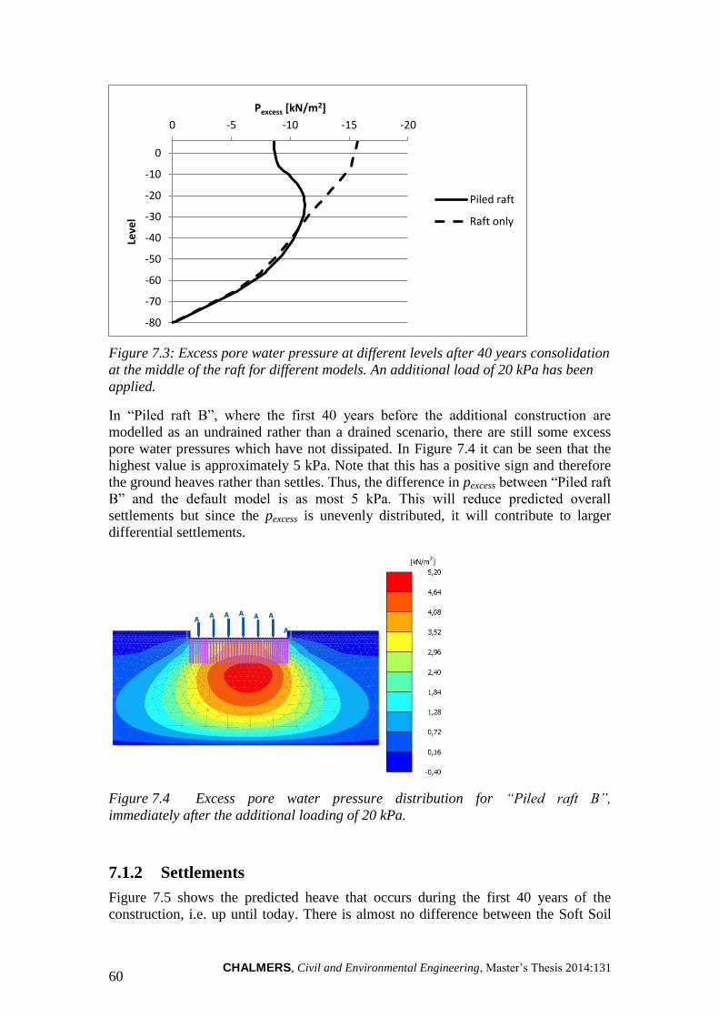
CHALMERS, Civil and Environmental Engineering, Master’s Thesis 2014:131 60
Figure 7.3: Excess pore water pressure at different levels after 40 years consolidation
at the middle of the raft for different models. An additional load of 20 kPa has been
applied.
In “Piled raft B”, where the first 40 years before the additional construction are
modelled as an undrained rather than a drained scenario, there are still some excess
pore water pressures which have not dissipated. In Figure 7.4 it can be seen that the
highest value is approximately 5 kPa. Note that this has a positive sign and therefore
the ground heaves rather than settles. Thus, the difference in pexcess between “Piled raft
B” and the default model is as most 5 kPa. This will reduce predicted overall
settlements but since the pexcess is unevenly distributed, it will contribute to larger
differential settlements.
Figure 7.4 Excess pore water pressure distribution for “Piled raft B”,
immediately after the additional loading of 20 kPa.
Settlements 7.1.2
Figure 7.5 shows the predicted heave that occurs during the first 40 years of the
construction, i.e. up until today. There is almost no difference between the Soft Soil
-80
-70
-60
-50
-40
-30
-20
-10
0
-20-15-10-50Le
vel
Pexcess [kN/m2]
Piled raft
Raft only
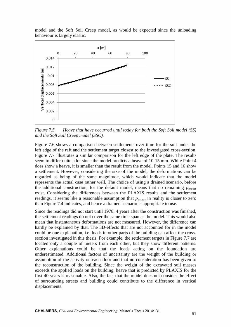
CHALMERS, Civil and Environmental Engineering, Master’s Thesis 2014:131 61
model and the Soft Soil Creep model, as would be expected since the unloading
behaviour is largely elastic.
Figure 7.5 Heave that have occurred until today for both the Soft Soil model (SS)
and the Soft Soil Creep model (SSC).
Figure 7.6 shows a comparison between settlements over time for the soil under the
left edge of the raft and the settlement target closest to the investigated cross-section.
Figure 7.7 illustrates a similar comparison for the left edge of the plate. The results
seem to differ quite a lot since the model predicts a heave of 10-15 mm. While Point 4
does show a heave, it is smaller than the result from the model. Points 15 and 16 show
a settlement. However, considering the size of the model, the deformations can be
regarded as being of the same magnitude, which would indicate that the model
represents the actual case rather well. The choice of using a drained scenario, before
the additional construction, for the default model, means that no remaining pexcess
exist. Considering the differences between the PLAXIS results and the settlement
readings, it seems like a reasonable assumption that pexcess in reality is closer to zero
than Figure 7.4 indicates, and hence a drained scenario is appropriate to use.
Since the readings did not start until 1978, 4 years after the construction was finished,
the settlement readings do not cover the same time span as the model. This would also
mean that instantaneous deformations are not measured. However, the difference can
hardly be explained by that. The 3D-effects that are not accounted for in the model
could be one explanation, i.e. loads in other parts of the building can affect the cross-
section investigated in this thesis. For example, the settlement targets in Figure 7.7 are
located only a couple of meters from each other, but they show different patterns.
Other explanations could be that the loads acting on the foundation are
underestimated. Additional factors of uncertainty are the weight of the building or
assumption of the activity on each floor and that no consideration has been given to
the reconstruction of the building. Since the weight of the excavated soil masses
exceeds the applied loads on the building, heave that is predicted by PLAXIS for the
first 40 years is reasonable. Also, the fact that the model does not consider the effect
of surrounding streets and building could contribute to the difference in vertical
displacements.
0
0,002
0,004
0,006
0,008
0,01
0,012
0,014
0 20 40 60 80 100
Ve
rtic
al d
isp
lace
me
nts
[m
]
x [m]
SS
SSC
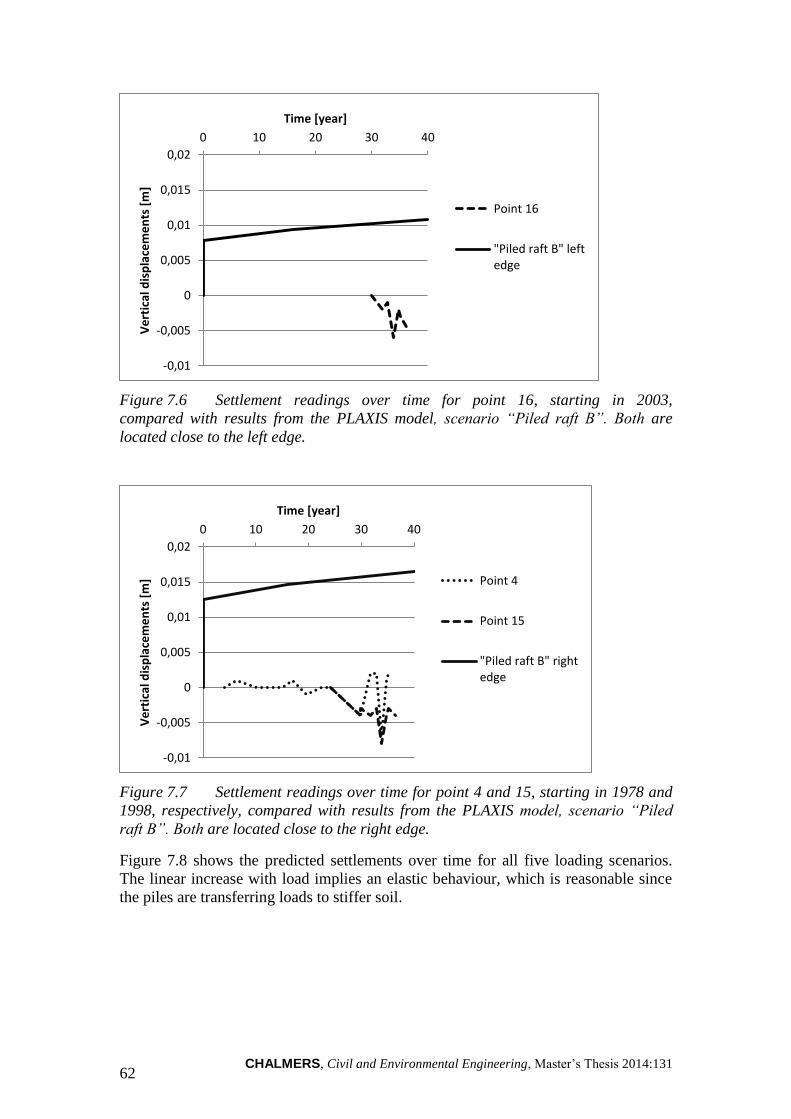
CHALMERS, Civil and Environmental Engineering, Master’s Thesis 2014:131 62
Figure 7.6 Settlement readings over time for point 16, starting in 2003,
compared with results from the PLAXIS model, scenario “Piled raft B”. Both are
located close to the left edge.
Figure 7.7 Settlement readings over time for point 4 and 15, starting in 1978 and
1998, respectively, compared with results from the PLAXIS model, scenario “Piled
raft B”. Both are located close to the right edge.
Figure 7.8 shows the predicted settlements over time for all five loading scenarios.
The linear increase with load implies an elastic behaviour, which is reasonable since
the piles are transferring loads to stiffer soil.
-0,01
-0,005
0
0,005
0,01
0,015
0,02
0 10 20 30 40V
ert
ical
dis
pla
cem
en
ts [
m]
Time [year]
Point 16
"Piled raft B" leftedge
-0,01
-0,005
0
0,005
0,01
0,015
0,02
0 10 20 30 40
Ve
rtic
al d
isp
lace
me
nts
[m
]
Time [year]
Point 4
Point 15
"Piled raft B" rightedge
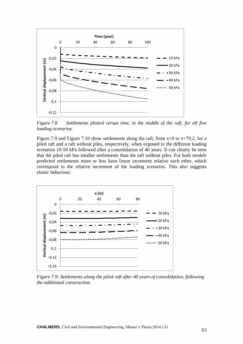
CHALMERS, Civil and Environmental Engineering, Master’s Thesis 2014:131 63
Figure 7.8 Settlements plotted versus time, in the middle of the raft, for all five
loading scenarios.
Figure 7.9 and Figure 7.10 show settlements along the raft, from x=0 to x=79,2, for a
piled raft and a raft without piles, respectively, when exposed to the different loading
scenarios 10-50 kPa followed after a consolidation of 40 years. It can clearly be seen
that the piled raft has smaller settlements than the raft without piles. For both models
predicted settlements more or less have linear increment relative each other, which
correspond to the relative increment of the loading scenarios. This also suggests
elastic behaviour.
Figure 7.9: Settlements along the piled raft after 40 years of consolidation, following
the additional construction.
-0,12
-0,1
-0,08
-0,06
-0,04
-0,02
0
0 20 40 60 80 100V
ert
ical
dis
pla
cem
en
t [m
]
Time [year]
10 kPa
20 kPa
30 kPa
40 kPa
50 kPa
-0,14
-0,12
-0,1
-0,08
-0,06
-0,04
-0,02
0
0 20 40 60 80
Ve
rtic
al d
isp
lace
me
nt
[m]
x [m]
10 kPa
20 kPa
30 kPa
40 kPa
50 kPa
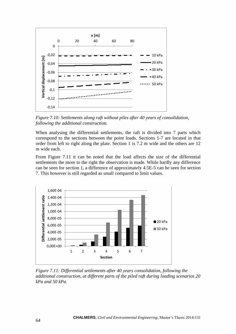
CHALMERS, Civil and Environmental Engineering, Master’s Thesis 2014:131 64
Figure 7.10: Settlements along raft without piles after 40 years of consolidation,
following the additional construction.
When analysing the differential settlements, the raft is divided into 7 parts which
correspond to the sections between the point loads. Sections 1-7 are located in that
order from left to right along the plate. Section 1 is 7.2 m wide and the others are 12
m wide each.
From Figure 7.11 it can be noted that the load affects the size of the differential
settlements the more to the right the observation is made. While hardly any difference
can be seen for section 1, a difference of approximately 4.5E-5 can be seen for section
7. This however is still regarded as small compared to limit values.
Figure 7.11: Differential settlements after 40 years consolidation, following the
additional construction, at different parts of the piled raft during loading scenarios 20
kPa and 50 kPa.
-0,14
-0,12
-0,1
-0,08
-0,06
-0,04
-0,02
0
0 20 40 60 80V
ert
ical
dis
pla
cem
en
t [m
]
x [m]
10 kPa
20 kPa
30 kPa
40 kPa
50 kPa
0,00E+00
2,00E-05
4,00E-05
6,00E-05
8,00E-05
1,00E-04
1,20E-04
1,40E-04
1,60E-04
1 2 3 4 5 6 7
Dif
fere
nti
al s
ett
lem
en
t ra
tio
Section
20 kPa
50 kPa
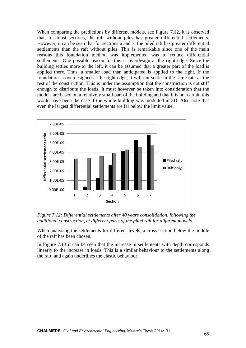
CHALMERS, Civil and Environmental Engineering, Master’s Thesis 2014:131 65
When comparing the predictions by different models, see Figure 7.12, it is observed
that, for most sections, the raft without piles has greater differential settlements.
However, it can be seen that for sections 6 and 7, the piled raft has greater differential
settlements than the raft without piles. This is remarkable since one of the main
reasons this foundation method was implemented was to reduce differential
settlements. One possible reason for this is overdesign at the right edge. Since the
building settles more to the left, it can be assumed that a greater part of the load is
applied there. Thus, a smaller load than anticipated is applied to the right. If the
foundation is overdesigned at the right edge, it will not settle in the same rate as the
rest of the construction. This is under the assumption that the construction is not stiff
enough to distribute the loads. It must however be taken into consideration that the
models are based on a relatively small part of the building and that it is not certain this
would have been the case if the whole building was modelled in 3D. Also note that
even the largest differential settlements are far below the limit value.
Figure 7.12: Differential settlements after 40 years consolidation, following the
additional construction, at different parts of the piled raft for different models.
When analysing the settlements for different levels, a cross-section below the middle
of the raft has been chosen.
In Figure 7.13 it can be seen that the increase in settlements with depth corresponds
linearly to the increase in loads. This is a similar behaviour to the settlements along
the raft, and again underlines the elastic behaviour.
0,00E+00
1,00E-05
2,00E-05
3,00E-05
4,00E-05
5,00E-05
6,00E-05
7,00E-05
1 2 3 4 5 6 7
Dif
fere
nti
al s
ett
lem
en
t ra
tio
Section
Piled raft
Raft only
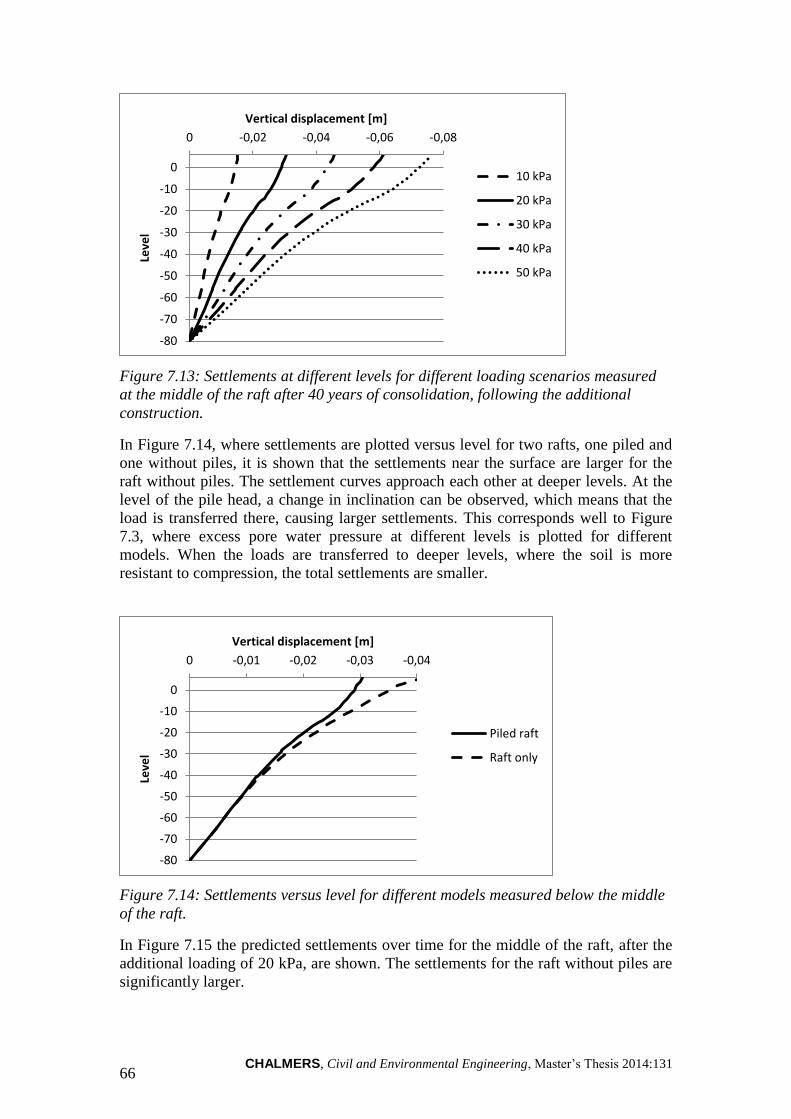
CHALMERS, Civil and Environmental Engineering, Master’s Thesis 2014:131 66
Figure 7.13: Settlements at different levels for different loading scenarios measured
at the middle of the raft after 40 years of consolidation, following the additional
construction.
In Figure 7.14, where settlements are plotted versus level for two rafts, one piled and
one without piles, it is shown that the settlements near the surface are larger for the
raft without piles. The settlement curves approach each other at deeper levels. At the
level of the pile head, a change in inclination can be observed, which means that the
load is transferred there, causing larger settlements. This corresponds well to Figure
7.3, where excess pore water pressure at different levels is plotted for different
models. When the loads are transferred to deeper levels, where the soil is more
resistant to compression, the total settlements are smaller.
Figure 7.14: Settlements versus level for different models measured below the middle
of the raft.
In Figure 7.15 the predicted settlements over time for the middle of the raft, after the
additional loading of 20 kPa, are shown. The settlements for the raft without piles are
significantly larger.
-80
-70
-60
-50
-40
-30
-20
-10
0
-0,08-0,06-0,04-0,020Le
vel
Vertical displacement [m]
10 kPa
20 kPa
30 kPa
40 kPa
50 kPa
-80
-70
-60
-50
-40
-30
-20
-10
0
-0,04-0,03-0,02-0,010
Leve
l
Vertical displacement [m]
Piled raft
Raft only

CHALMERS, Civil and Environmental Engineering, Master’s Thesis 2014:131 67
Figure 7.15: Settlements at different times after the additional load of 20 kPa,
obtained at the middle of the raft. The timespan observed is 0-100 years, since this is
the technical lifespan for buildings.
Soft Soil Creep
Figure 7.16, Figure 7.17 and Figure 7.18 show how settlements by time and level
differ for the two material models Soft soil and Soft Soil Creep.
When evaluating µ* from the oedometer tests, the inclination of the curves might be
too steep to get the proper µ* value. It is important to evaluate the parameter when the
primary consolidation has ended and any effects of structure (for sensitive soils) are
no longer present (i.e. pure creep at hign stress levels). If consolidation is still
occurring, it might overestimate µ* and thus contribute to that larger settlements
being predicted, than will actually happen. Looking at the inclination of the curves in
Appendix C, it is hard to tell if consolidation is still occurring. However, the
settlement over time for the Soft Soil Creep model indicates that it occur very little
creep during the first 100 years. Also, when applying the Soft Soil Creep model on the
time span up until today, the difference in heave is negligible. This is logical for low
loads, since if studying the stress analysis graph, see Figure 7.35, the stress level
should be below the creep limit when the piles are transferring some of the applied
loads to a greater depth. However, it is a bit more remarkable that there is no
significant creep during the first 100 years when applying a load of 50 kPa. The
results above point at elastic response of the soil.
In Figure 7.17 “SSC – control” is plotted. It is a point located at the surface at a
relatively large distance from the raft, and is not exposed to any load elements. As can
be seen the deformation will with time be larger than the ones predicted below the
raft. This is caused by an error in the formulation of the Soft Soil Creep model. Due to
heave at the excavation, the soil located there behaves more elastically than the soil
not located at the excavation. This indicates that the Soft Soil Creep model
overestimates the time dependent settlements and hence the model does not consider
the creep deformations in a realistic way.
-0,06
-0,05
-0,04
-0,03
-0,02
-0,01
0
0 20 40 60 80 100V
ert
ical
dis
pla
cem
en
t [m
]
Time [year]
Piled Raft
Raft only
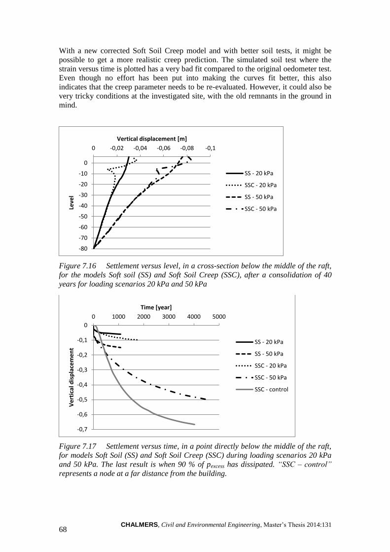
CHALMERS, Civil and Environmental Engineering, Master’s Thesis 2014:131 68
With a new corrected Soft Soil Creep model and with better soil tests, it might be
possible to get a more realistic creep prediction. The simulated soil test where the
strain versus time is plotted has a very bad fit compared to the original oedometer test.
Even though no effort has been put into making the curves fit better, this also
indicates that the creep parameter needs to be re-evaluated. However, it could also be
very tricky conditions at the investigated site, with the old remnants in the ground in
mind.
Figure 7.16 Settlement versus level, in a cross-section below the middle of the raft,
for the models Soft soil (SS) and Soft Soil Creep (SSC), after a consolidation of 40
years for loading scenarios 20 kPa and 50 kPa
Figure 7.17 Settlement versus time, in a point directly below the middle of the raft,
for models Soft Soil (SS) and Soft Soil Creep (SSC) during loading scenarios 20 kPa
and 50 kPa. The last result is when 90 % of pexcess has dissipated. “SSC – control”
represents a node at a far distance from the building.
-80
-70
-60
-50
-40
-30
-20
-10
0
-0,1-0,08-0,06-0,04-0,020
Leve
l
Vertical displacement [m]
SS - 20 kPa
SSC - 20 kPa
SS - 50 kPa
SSC - 50 kPa
-0,7
-0,6
-0,5
-0,4
-0,3
-0,2
-0,1
0
0 1000 2000 3000 4000 5000
Ve
rtic
al d
isp
lace
me
nt
Time [year]
SS - 20 kPa
SS - 50 kPa
SSC - 20 kPa
SSC - 50 kPa
SSC - control
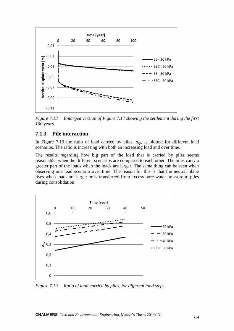
CHALMERS, Civil and Environmental Engineering, Master’s Thesis 2014:131 69
Figure 7.18 Enlarged version of Figure 7.17 showing the settlement during the first
100 years.
Pile interaction 7.1.3
In Figure 7.19 the ratio of load carried by piles, αrp, is plotted for different load
scenarios. The ratio is increasing with both an increasing load and over time.
The results regarding how big part of the load that is carried by piles seems
reasonable, when the different scenarios are compared to each other. The piles carry a
greater part of the loads when the loads are larger. The same thing can be seen when
observing one load scenario over time. The reason for this is that the neutral plane
rises when loads are larger or is transferred from excess pore water pressure to piles
during consolidation.
Figure 7.19 Ratio of load carried by piles, for different load steps
-0,11
-0,09
-0,07
-0,05
-0,03
-0,01
0,01
0 20 40 60 80 100V
ert
ical
dis
pla
cem
en
t [m
]
Time [year]
SS - 20 kPa
SSC - 20 kPa
SS - 50 kPa
SSC - 50 kPa
0
0,1
0,2
0,3
0,4
0,5
0,6
0 10 20 30 40 50
αrp
Time [year]
20 kPa
30 kPa
40 kPa
50 kPa
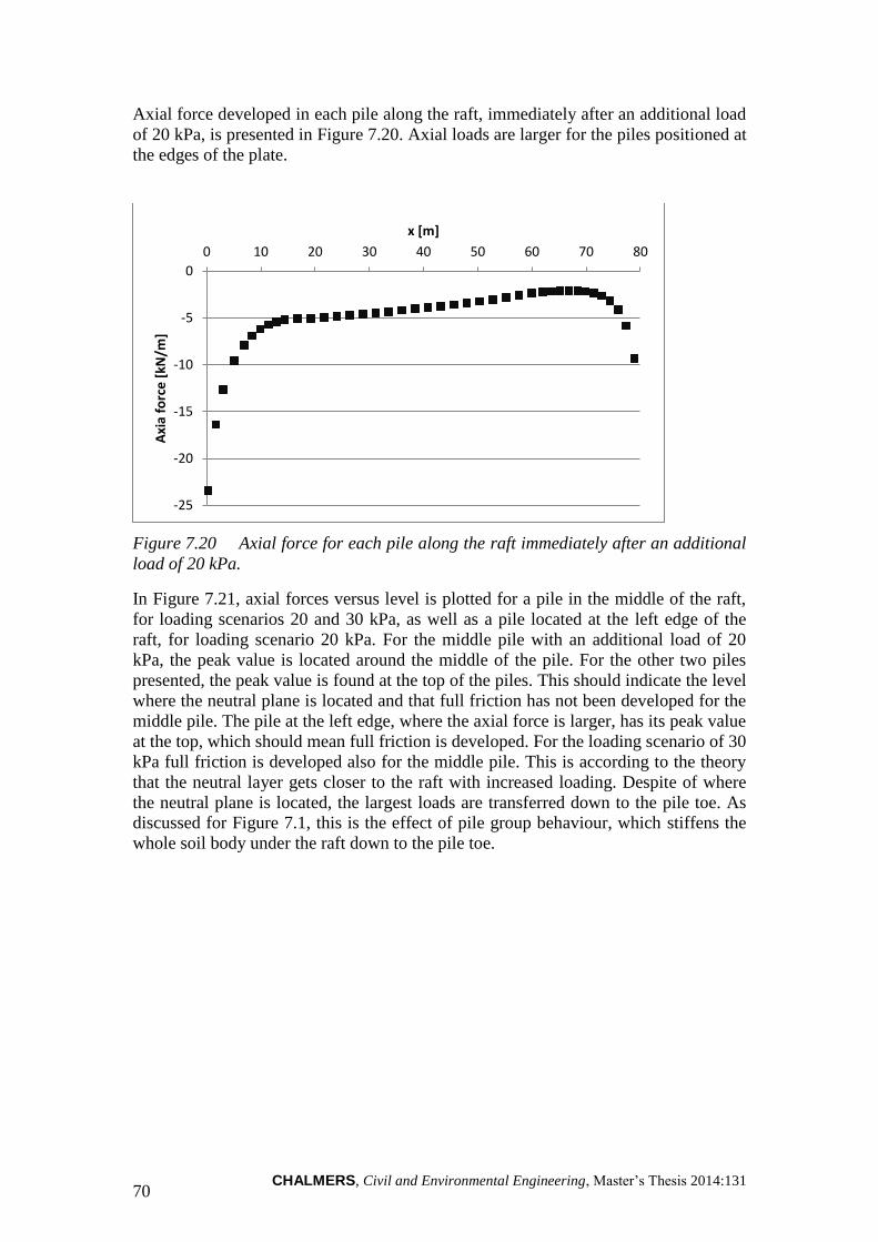
CHALMERS, Civil and Environmental Engineering, Master’s Thesis 2014:131 70
Axial force developed in each pile along the raft, immediately after an additional load
of 20 kPa, is presented in Figure 7.20. Axial loads are larger for the piles positioned at
the edges of the plate.
Figure 7.20 Axial force for each pile along the raft immediately after an additional
load of 20 kPa.
In Figure 7.21, axial forces versus level is plotted for a pile in the middle of the raft,
for loading scenarios 20 and 30 kPa, as well as a pile located at the left edge of the
raft, for loading scenario 20 kPa. For the middle pile with an additional load of 20
kPa, the peak value is located around the middle of the pile. For the other two piles
presented, the peak value is found at the top of the piles. This should indicate the level
where the neutral plane is located and that full friction has not been developed for the
middle pile. The pile at the left edge, where the axial force is larger, has its peak value
at the top, which should mean full friction is developed. For the loading scenario of 30
kPa full friction is developed also for the middle pile. This is according to the theory
that the neutral layer gets closer to the raft with increased loading. Despite of where
the neutral plane is located, the largest loads are transferred down to the pile toe. As
discussed for Figure 7.1, this is the effect of pile group behaviour, which stiffens the
whole soil body under the raft down to the pile toe.
-25
-20
-15
-10
-5
0
0 10 20 30 40 50 60 70 80
Axi
a fo
rce
[kN
/m]
x [m]
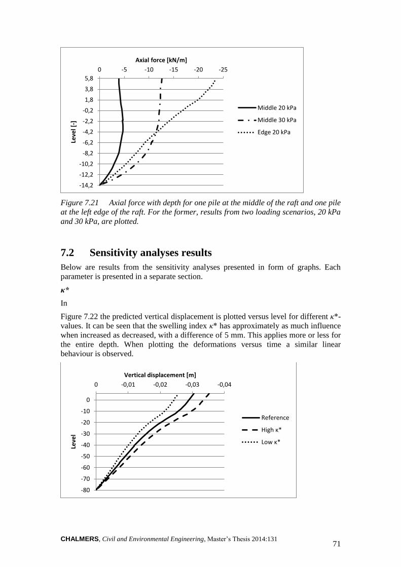
CHALMERS, Civil and Environmental Engineering, Master’s Thesis 2014:131 71
Figure 7.21 Axial force with depth for one pile at the middle of the raft and one pile
at the left edge of the raft. For the former, results from two loading scenarios, 20 kPa
and 30 kPa, are plotted.
7.2 Sensitivity analyses results
Below are results from the sensitivity analyses presented in form of graphs. Each
parameter is presented in a separate section.
κ*
In
Figure 7.22 the predicted vertical displacement is plotted versus level for different κ*-
values. It can be seen that the swelling index κ* has approximately as much influence
when increased as decreased, with a difference of 5 mm. This applies more or less for
the entire depth. When plotting the deformations versus time a similar linear
behaviour is observed.
-14,2
-12,2
-10,2
-8,2
-6,2
-4,2
-2,2
-0,2
1,8
3,8
5,8
-25-20-15-10-50Le
vel [
-]
Axial force [kN/m]
Middle 20 kPa
Middle 30 kPa
Edge 20 kPa
-80
-70
-60
-50
-40
-30
-20
-10
0
-0,04-0,03-0,02-0,010
Leve
l
Vertical displacement [m]
Reference
High κ*
Low κ*
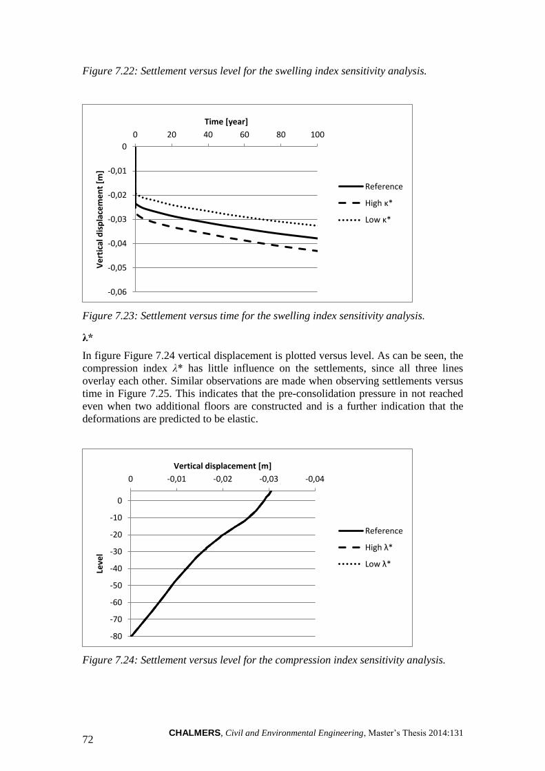
CHALMERS, Civil and Environmental Engineering, Master’s Thesis 2014:131 72
Figure 7.22: Settlement versus level for the swelling index sensitivity analysis.
Figure 7.23: Settlement versus time for the swelling index sensitivity analysis.
λ*
In figure Figure 7.24 vertical displacement is plotted versus level. As can be seen, the
compression index λ* has little influence on the settlements, since all three lines
overlay each other. Similar observations are made when observing settlements versus
time in Figure 7.25. This indicates that the pre-consolidation pressure in not reached
even when two additional floors are constructed and is a further indication that the
deformations are predicted to be elastic.
Figure 7.24: Settlement versus level for the compression index sensitivity analysis.
-0,06
-0,05
-0,04
-0,03
-0,02
-0,01
0
0 20 40 60 80 100
Ve
rtic
al d
isp
lace
me
nt
[m]
Time [year]
Reference
High κ*
Low κ*
-80
-70
-60
-50
-40
-30
-20
-10
0
-0,04-0,03-0,02-0,010
Leve
l
Vertical displacement [m]
Reference
High λ*
Low λ*

CHALMERS, Civil and Environmental Engineering, Master’s Thesis 2014:131 73
Figure 7.25: Settlement versus time for the compression index sensitivity analysis.
OCR
In Figure 7.26 and Figure 7.27 it can be seen that an increase in the value of the over
consolidation ratio has no significant effect on the settlements. When the soil
however, is set to be normal consolidated a difference is relatively large
(approximately 9 mm at the top).
Figure 7.26: Settlement versus level for the over consolidation ratio sensitivity
analysis.
-0,06
-0,05
-0,04
-0,03
-0,02
-0,01
0
0 20 40 60 80 100V
ert
ical
dis
pla
cem
en
t [m
]
Time [year]
Reference
High λ*
Low λ*
-80
-70
-60
-50
-40
-30
-20
-10
0
-0,04-0,03-0,02-0,010
Leve
l
Vertical displacement [m]
Reference
High OCR*
Low OCR*
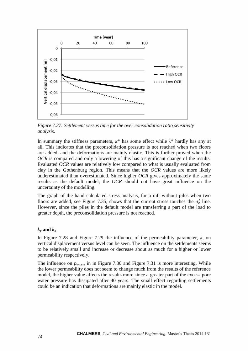
CHALMERS, Civil and Environmental Engineering, Master’s Thesis 2014:131 74
Figure 7.27: Settlement versus time for the over consolidation ratio sensitivity
analysis.
In summary the stiffness parameters, κ* has some effect while λ* hardly has any at
all. This indicates that the preconsolidation pressure is not reached when two floors
are added, and the deformations are mainly elastic. This is further proved when the
OCR is compared and only a lowering of this has a significant change of the results.
Evaluated OCR values are relatively low compared to what is usually evaluated from
clay in the Gothenburg region. This means that the OCR values are more likely
underestimated than overestimated. Since higher OCR gives approximately the same
results as the default model, the OCR should not have great influence on the
uncertainty of the modelling.
The graph of the hand calculated stress analysis, for a raft without piles when two
floors are added, see Figure 7.35, shows that the current stress touches the line.
However, since the piles in the default model are transferring a part of the load to
greater depth, the preconsolidation pressure is not reached.
ky and kx
In Figure 7.28 and Figure 7.29 the influence of the permeability parameter, k, on
vertical displacement versus level can be seen. The influence on the settlements seems
to be relatively small and increase or decrease about as much for a higher or lower
permeability respectively.
The influence on pexcess in in Figure 7.30 and Figure 7.31 is more interesting. While
the lower permeability does not seem to change much from the results of the reference
model, the higher value affects the results more since a greater part of the excess pore
water pressure has dissipated after 40 years. The small effect regarding settlements
could be an indication that deformations are mainly elastic in the model.
-0,06
-0,05
-0,04
-0,03
-0,02
-0,01
0
0 20 40 60 80 100V
ert
ical
dis
pla
cem
en
t [m
]
Time [year]
Reference
High OCR
Low OCR
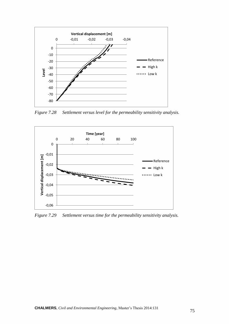
CHALMERS, Civil and Environmental Engineering, Master’s Thesis 2014:131 75
Figure 7.28 Settlement versus level for the permeability sensitivity analysis.
Figure 7.29 Settlement versus time for the permeability sensitivity analysis.
-80
-70
-60
-50
-40
-30
-20
-10
0
-0,04-0,03-0,02-0,010Le
vel
Vertical displacement [m]
Reference
High k
Low k
-0,06
-0,05
-0,04
-0,03
-0,02
-0,01
0
0 20 40 60 80 100
Ve
rtic
al d
isp
lace
me
nt
[m]
Time [year]
Reference
High k
Low k
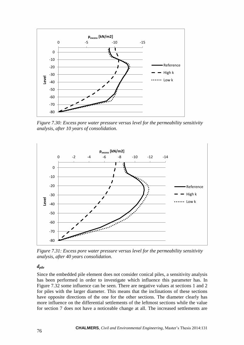
CHALMERS, Civil and Environmental Engineering, Master’s Thesis 2014:131 76
Figure 7.30: Excess pore water pressure versus level for the permeability sensitivity
analysis, after 10 years of consolidation.
Figure 7.31: Excess pore water pressure versus level for the permeability sensitivity
analysis, after 40 years consolidation.
dpile
Since the embedded pile element does not consider conical piles, a sensitivity analysis
has been performed in order to investigate which influence this parameter has. In
Figure 7.32 some influence can be seen. There are negative values at sections 1 and 2
for piles with the larger diameter. This means that the inclinations of these sections
have opposite directions of the one for the other sections. The diameter clearly has
more influence on the differential settlements of the leftmost sections while the value
for section 7 does not have a noticeable change at all. The increased settlements are
-80
-70
-60
-50
-40
-30
-20
-10
0
-15-10-50Le
vel
pexcess [kN/m2]
Reference
High k
Low k
-80
-70
-60
-50
-40
-30
-20
-10
0
-14-12-10-8-6-4-20
Leve
l
pexcess [kN/m2]
Reference
High k
Low k

CHALMERS, Civil and Environmental Engineering, Master’s Thesis 2014:131 77
still very small when compared to the limit values. It is hard to tell which diameter
gives a more correct result without real pile test to compare with. Such tests should be
performed in order to evaluate how to model conical piles with the embedded pile row
element.
Figure 7.32: Differential settlements for different dpile input values.
Lspacing
In Figure 7.33 in can be seen that Lspacing does not have any significant influence on
the differential settlements.
,
Figure 7.33: Differential settlements for different Lspacing input values.
-2,00E-05
-1,00E-05
0,00E+00
1,00E-05
2,00E-05
3,00E-05
4,00E-05
5,00E-05
6,00E-05
7,00E-05
1 2 3 4 5 6 7
Dif
fere
nti
al s
ett
lem
en
t ra
tio
Section
Reference
dpile = 0.125
dpile = 0.285
-2,00E-05
-1,00E-05
0,00E+00
1,00E-05
2,00E-05
3,00E-05
4,00E-05
5,00E-05
6,00E-05
7,00E-05
1 2 3 4 5 6 7
Dif
fere
nti
al s
ett
lem
en
t ra
tio
Section
Reference
Lspacing = 1.7
Lspacing = 1.9
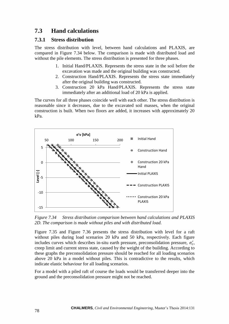
CHALMERS, Civil and Environmental Engineering, Master’s Thesis 2014:131 78
7.3 Hand calculations
Stress distribution 7.3.1
The stress distribution with level, between hand calculations and PLAXIS, are
compared in Figure 7.34 below. The comparison is made with distributed load and
without the pile elements. The stress distribution is presented for three phases.
1. Initial Hand/PLAXIS. Represents the stress state in the soil before the
excavation was made and the original building was constructed.
2. Construction Hand/PLAXIS. Represents the stress state immediately
after the original building was constructed.
3. Construction 20 kPa Hand/PLAXIS. Represents the stress state
immediately after an additional load of 20 kPa is applied.
The curves for all three phases coincide well with each other. The stress distribution is
reasonable since it decreases, due to the excavated soil masses, when the original
construction is built. When two floors are added, it increases with approximately 20
kPa.
Figure 7.34 Stress distribution comparison between hand calculations and PLAXIS
2D. The comparison is made without piles and with distributed load.
Figure 7.35 and Figure 7.36 presents the stress distribution with level for a raft
without piles during load scenarios 20 kPa and 50 kPa, respectively. Each figure
includes curves which describes in-situ earth pressure, preconsolidation pressure, ,
creep limit and current stress state, caused by the weight of the building. According to
these graphs the preconsolidation pressure should be reached for all loading scenarios
above 20 kPa in a model without piles. This is contradictive to the results, which
indicate elastic behaviour for all loading scenarios.
For a model with a piled raft of course the loads would be transferred deeper into the
ground and the preconsolidation pressure might not be reached.
-15
-10
-5
0
5
50 100 150 200
Leve
l [-]
σ'v [kPa] Initial Hand
Construction Hand
Construction 20 kPaHand
Initial PLAXIS
Construction PLAXIS
Construction 20 kPaPLAXIS
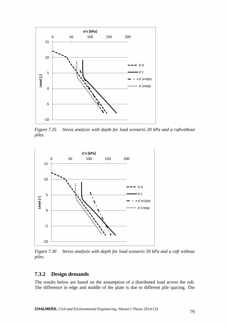
CHALMERS, Civil and Environmental Engineering, Master’s Thesis 2014:131 79
Figure 7.35 Stress analysis with depth for load scenario 20 kPa and a raftwithout
piles.
Figure 7.36 Stress analysis with depth for load scenario 50 kPa and a raft without
piles.
Design demands 7.3.2
The results below are based on the assumption of a distributed load across the raft.
The difference in edge and middle of the plate is due to different pile spacing. The
-10
-5
0
5
10
15
0 50 100 150 200Le
vel [
-]
σ'v [kPa]
σ´o
σ´c
σ´o+Δσz
σ´creep
-10
-5
0
5
10
15
0 50 100 150 200
Leve
l [-]
σ'v [kPa]
σ´o
σ´c
σ´o+Δσz
σ´creep
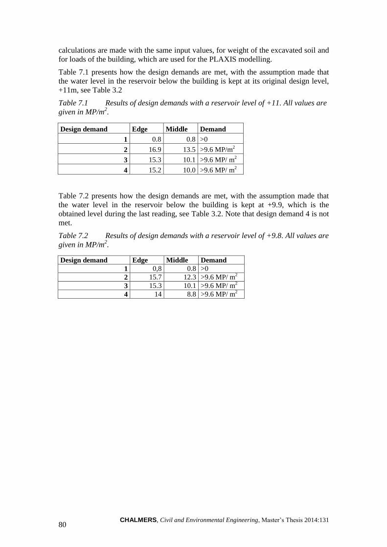
CHALMERS, Civil and Environmental Engineering, Master’s Thesis 2014:131 80
calculations are made with the same input values, for weight of the excavated soil and
for loads of the building, which are used for the PLAXIS modelling.
Table 7.1 presents how the design demands are met, with the assumption made that
the water level in the reservoir below the building is kept at its original design level,
+11m, see Table 3.2
Table 7.1 Results of design demands with a reservoir level of +11. All values are
given in MP/m2.
Design demand Edge Middle Demand
1 0.8 0.8 >0
2 16.9 13.5 >9.6 MP/m2
3 15.3 10.1 >9.6 MP/ m2
4 15.2 10.0 >9.6 MP/ m2
Table 7.2 presents how the design demands are met, with the assumption made that
the water level in the reservoir below the building is kept at +9.9, which is the
obtained level during the last reading, see Table 3.2. Note that design demand 4 is not
met.
Table 7.2 Results of design demands with a reservoir level of +9.8. All values are
given in MP/m2.
Design demand Edge Middle Demand
1 0,8 0.8 >0
2 15.7 12.3 >9.6 MP/ m2
3 15.3 10.1 >9.6 MP/ m2
4 14 8.8 >9.6 MP/ m2
CHALMERS, Civil and Environmental Engineering, Master’s Thesis 2014:131 81
8 Discussion
This chapter contains discussion regarding general aspects of the model and the thesis
as a whole.
No consideration has been taken to the group effect of the piles, when calculating the
input value for the skin friction. It was difficult to know beforehand how the modelled
piles would behave, but since the behavior seems to correspond to a pile group, this
needs to be considered in further analysis. Since the behaviour of a pile element is a
3D problem, it is of course difficult to model it in a 2D model. Since there is little
literature to find regarding the embedded pile row element, it is difficult to interpret
how accurate it is working. Based on our results, the pile elements seem to behave in
reasonable way. However, real pile tests needs to be performed in order to validate
their function.
When observing the comparisons between results from different loading scenarios it
can be seen that total settlements, both by time and depth, seem to correspond to the
increase in loads in a linear manner. The differential settlements at the right most
sections of the piled raft have a greater increase than the left edge. Since these still are
quite small, compared to maximum allowed values, it is likely that total settlements at
connections with the surrounding streets will be decisive for whether further
construction can be made. Since the surroundings have not been considered in this
thesis, only speculation can be made, but of course if the settlements at the
connections are too large, it could lead to problems with for example pipes, cables or
cracking of joints.
In this specific case, it is hard to predict the stiffness of the ground only from soil
tests, since there are old remnants there from old construction, e.g. old timber piles. It
is difficult to predict how this would affect the construction of additional floors. A
logical reasoning would be that it reduces the settlements since the soil gets stiffer.
But irregular stiffness might also cause differential settlements.
There are several uncertainties and simplifications to consider regarding the
evaluations and calculations performed. One of the most obvious is of course the
choice of modelling in 2D. Since a plane strain model would over- rather than
underestimate settlements, there might be more capacity of the foundation than these
calculations indicate.
The data which the geological and hydrological conditions are based on are old and
the equipment used for obtaining them might not be as good as the ones used today.
The lack of triaxial tests has also resulted in the need to assume key parameters. Real
triaxial tests should be performed, since they should give a better foundation than
using relationships to evaluate results from one-dimensional oedometer tests together
with assumptions. The construction drawings are from the 1970’s. It might be needed
to recalculate the loads since there has been some reconstruction of the building and
relocation of former activities.
No parametric study regarding ϕ’ has been performed, but the value used when
modelling is somewhat lower than average for clay in Gothenburg, which means the
calculations are conservative. For further investigation the influence of ϕ’ should be
considered.
A scenario where the water level in the reservoirs below the building would
drastically sink has not been considered. This partly because it is difficult to model
CHALMERS, Civil and Environmental Engineering, Master’s Thesis 2014:131 82
and time is restricted. A simplification of a scenario would be that for each meter the
water level is lowered, 10 kPa is added as an applied load on foundation. Thus, by
simulating a total addition of five floors, we have also simulated a scenario where the
water level drops five meter. For further studies investigations regarding a possible
increase in ground water level should also be carried out.
The model does not include the non-hydrostatic over pressure of pore water, 20-30
kPa at 20 meters depth. This is because there has not been very detailed information
about this, for example how it increases with depth and at which depth it starts.
An error made during simulation was that only embedded pile row elements with
Lspacing = 1.5 m were used. Some piles in the middle should have been given input
value Lspacing = 1.9 m. This was noticed late in the investigations and because of the
time frame there was no time to redo all calculations. However this only affects the
spacing in the out of plane direction. The parametric analysis of Lspacing show that
there was little influence regarding differential settlements. The αrp value would
probably have been slightly reduced if the middle piled would have had the larger
Lspacing value, since fewer piles would increase the contact stress between ground and
raft.
According to our calculations, the design values are not fulfilled today. It should be
noted that they are made with our evaluation of loads, which could differ from the
original, since we have not been able to find the old calculations for building 6.
The analysis does not consider any time aspect for construction phases. This might
lead to prediction of larger instant settlements than if the load from construction
phases would have been applied over time.

CHALMERS, Civil and Environmental Engineering, Master’s Thesis 2014:131 83
9 Conclusions
Below conclusions drawn from the results and the discussion are presented.
The aim of this project has been to investigate the foundation principle of a piled raft
and how well this can be modelled with numerical analysis, using a plane strain model
and the embedded pile row element, in the computer software PLAXIS 2D. A case
study model has been made of the building Nordstaden 8:27, where geotechnical
effects, in terms of settlement caused by additional construction, is investigated.
The model in this case study seems to work in a fairly reasonable manner, considering
the magnitude of settlements. This indicates that a plane strain model in PLAXIS 2D
can be a good and time effective tool to get a first result, before using a more
complicated three-dimensional model.
Using the embedded pile row element to model the behavior of piles seems to give
qualitatively reasonable results in our model. However, real pile tests need to be
performed in order to validate their behavior.
For further investigations, Nordstaden 8:27 should be modeled in 3D. A piled raft is a
very complex foundation method and in 2D there are too many 3D interactions and
factors of uncertainty to be able to fully trust the results. Surrounding buildings and
streets would also have to be taken into consideration. It might also be needed to
make calculations based on newer construction drawings for loads acting on the
foundation.
New soil tests, especially triaxial tests and a new evaluation of the permeability, need
to be performed. The soil tests used in this thesis are from 1966, which makes it hard
to validate their reliability. Due to the lack of a triaxial test, some parameters have
been approximated for this case study, which have added an uncertainty factor to the
model.
The magnitude of the differential settlements is very low compared to the limit values,
for all the modeled loading scenarios. Therefore, differential settlements should not
cause any problems. Since Nordstaden 8:27 is connected to the surrounding streets, it
is instead the settlements at the edges of the raft that will be decisive for how many
floors that can be added. Further studies should investigate how much settlements can
be allowed without causing too much cracking in the connection or any damage to the
reservoirs or sensitive parts below the building.
CHALMERS, Civil and Environmental Engineering, Master’s Thesis 2014:131 84
10 References
Alén, C. (2012) Pile foundations - Short handbook (Educational material in
Geotechnics), Gothenburg: Chalmers University of Technology.
Bergdahl, U., Malmborg, B.S. and Ottosson, E. (1993) Plattgrundläggning, Solna:
AB Svensk Byggtjänst.
Boverket (2004) Boverkets handbok om betongkonstruktioner BBK 04.
Carling et al, O. (1992) Dimensionering av träkonstruktioner, Stockholm: AB Svensk
Byggtjänst and Trätek.
Chai, J.C., Huang, J.Z. and Wu, W.J. (2002) 'Interaction between pile and raft in piled
raft foundation', Advances in Building Technology, Hong Kong, 603-610.
Craig, R.F. and Knappet, J.A. (2012) Craig's soil mechanics, 8th
edition, Abingdon:
Spon Press.
Eriksson, P., Jendeby, L., Olsson, T. and Svensson, T. (2004) Commission on Pile
Research: Report 100 - Cohesion Piles, Linköping: Swedens Geotechnical Institute
(SGI).
Fellenius, B.H. (2004) 'Unified design of piled foundations with emphasis on
settlement analysis', Geo-Institute Geo-TRANS Conference, Los Angeles, 253-275.
Fellenius, B.H. (2006) Basics of Foundation Design, Calgary.
Flemming, W.G.K., Weltman, A.J., Randolph, M.F. and Elson, W.K. (1992) Piling
engineering, 2nd
edition, Glasgow and London: Blackie and Son Ltd.
Fredriksson, A. and Rosén, R. (1988) 'Kryppålar och bottenplatta - Hållbart alternativ
på besvärlig mark', Byggindustrin, No 34.
Fritz, M. (1997) Nordstan - Från gårdagens vision till dagens affärscentrum,
Gothenburg: Tre Böcker Förlag AB.
Gibson, R.E., Gobert, A. and Schiffman, R.L. (1990) 'On Cryer's problem with large
displacements and variable permeability', Géotechnique 40, No. 4, pp. 627-631.
Giretti, D. (2009) Modelling of piled raft foundations in sand, Ferrara: University of
Ferrara.
Gustafsson, L., Gustavsson, T., Lund, R., Lüsch, K., Röine, H., Tauson, S.,
Söderquist, J. and Waldenström, L. (n.d) Objekt 6 i Östra Nordstan, Gothenburg:
Artmen ab.
Hansbo, S. (1989) Grundläggning av byggnader och maskinfundament, 2nd
edition,
Gothenburg: Chalmers University of Technology.
Hansbo, S., Hoffman, E. and Mosesson, J. (1973) 'Östra Nordstaden, Gothenburg.
Experiences concerning a difficult foundation problem and its unorthodox solution',
Procedings ot the eighth international conference on soil mechanics and foundation
engineering, Moscow, 105-110.
Hansbo, S. and Jedenby, L. (1998) 'A follow-up of two different foundation
principles', Fourth International Conference on Case Histories Geotechnical
Engineering, St. Louis, Missouri, 259-264.

CHALMERS, Civil and Environmental Engineering, Master’s Thesis 2014:131 85
Hansbo, S. and Källström, R. (1983) 'Creep piles - a cost-effective alternative to
conventional friction piles', Väg- och vattenbyggaren, No 7-8.
Helenelund, K.V. (1977) Methods for reducing undrained shear strength of clay. SGI
report 3., Linköping: Swedish Geotechnical Institute.
Holm, G. and Olsson, C. (1993) Pålgrundläggning, Solna: AB Svensk Byggtjänst.
Holtz, R.D. (1991) Foundation Engineering Handbook, New York: Van Nostrand
Reinhold.
Jedenby, L. (1986b) 'Grundlägg inte på pålar - utan med hjälp av pålar', Väg- och
vattenbyggaren, No 3, pp. 21-23.
Jendeby, L. (1986a) Friction piled foundations in soft clay - A study of load transfer
and settlements, Gothenburg: Chalmers University of Technology.
Katzenbach, R., Gutberlet, C. and Bachmann, G. (2007) 'Soil-Structure Interaction
aspects for ultimate limit state design of complex foundations', First International
Symposium on Geotechnical Safety & Risk, Shanghai, 585-596.
Kulhawy, F.H. and Prakoso, W.A. (2001) 'Contribution to piles raft foundation
design', Journal of geotechnical and geoenvironmental engineering, January, pp. 17-
24.
Larsson, R. (1986) Consolidation of soft soils, Linköping: Swedish Geotechnical
Institute (SGI).
Larsson, R. (2008) Soil properties, Linköping: Swedish Geotechnical Institute (SGI).
Leoni, M., Karstunen, M. and Vermeer, P.A. (2008) 'Anisotropic creep model for soft
soils', Géotechnique 58, No. 3, pp. 215-226.
Nguyen, D.D.C., Jo, S.-B. and Kim, D.-S. (2013) 'Design method of piled-raft
foundations under vertical load considering interaction effect', Computers and
Geotechnics 47, pp. 16-27.
Olsson, M. (2010) Calculating long-term settlement in soft clays - with special focus
on the Gothenburg region, Linköping: Swedish Geotechnical Institute (SGI).
PLAXIS (2012) Embedded pile row: A case study in PLAXIS 2D, 6 November,
[Online], Available: http://kb.plaxis.nl/sites/kb.plaxis.nl/files/kb-
publications/CaseStudy_embedded_pile_row_nov2012_0.pdf [16 June 2014].
PLAXIS (2014a) Material Models Manual, [Online], Available:
http://www.plaxis.nl/files/files/2DAnniversaryEdition-3-Material-Models.pdf [03 Jun
2014].
PLAXIS (2014b) Reference Manual, [Online], Available:
http://www.plaxis.nl/files/files/2DAnniversaryEdition-2-Reference.pdf [03 Jun 2014].
PLAXIS (2014c) Embedded Pile Row in Plaxis 2D, 16 Jun, [Online], Available:
http://kb.plaxis.nl/sites/kb.plaxis.nl/files/kb-
publications/CaseStudy_embedded_pile_row_nov2012_0.pdf [16 Jun 2014].
Poulos, H.G. (2001) METHODS OF ANALYSIS OF PILED RAFT FOUNDATIONS,
Sydney: Coffey Geosciences Pty. Ltd. & The University of Sydney.
CHALMERS, Civil and Environmental Engineering, Master’s Thesis 2014:131 86
Sluis, J., Besseling, F., Stuurwold, P. and Lengkeek, A. (2013) 'Validation and
Application of the Embedded Pile Row-feature in PLAXIS 2D', Plaxis Bulletin, Issue
34, pp. 10-13.
Statens planverk (1968) Svensk Byggnorm 67 (SBN 1967), Stockholm.
Svensson, L. (1993) Östra Nordstan, Göteborg - Grundvattennivåer och sättningar,
Gothenburg: J&W Bygg & Anläggning AB.
Waterman, D. (2006) Structural elements and excavations, Chile: Plaxis.
Waterman, D. and Broere, W. (2005) Practical application of the Soft Soil Creep
model - Part III, Delft: Delft University of Technology / Plaxis BV.
Wood, D.M. (1990) Soil behaviour and critical state soil mechanics, Cambridge:
Press Syndicate of the University of Cambridge.
CHALMERS, Civil and Environmental Engineering, Master’s Thesis 2014:131 87
Appendices
Appendix A – Construction drawings
Appendix B – Hand calculations
Appendix C- Soil test evaluations
Appendix D – Continous beams with uniformly distributed loads –
Sectional forces
Appendix E – Settlement limits
Appendix F – Settlement readings
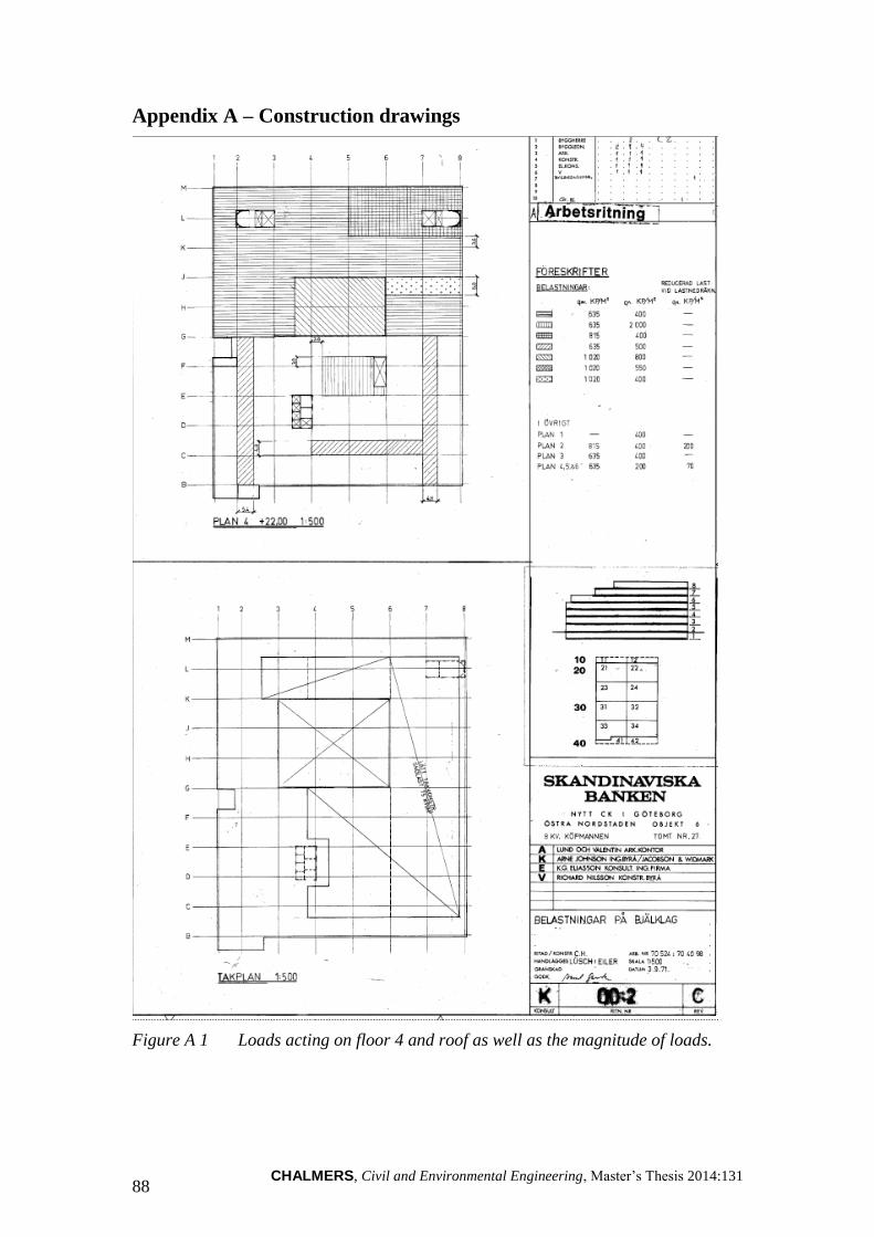
CHALMERS, Civil and Environmental Engineering, Master’s Thesis 2014:131 88
Appendix A – Construction drawings
Figure A 1 Loads acting on floor 4 and roof as well as the magnitude of loads.
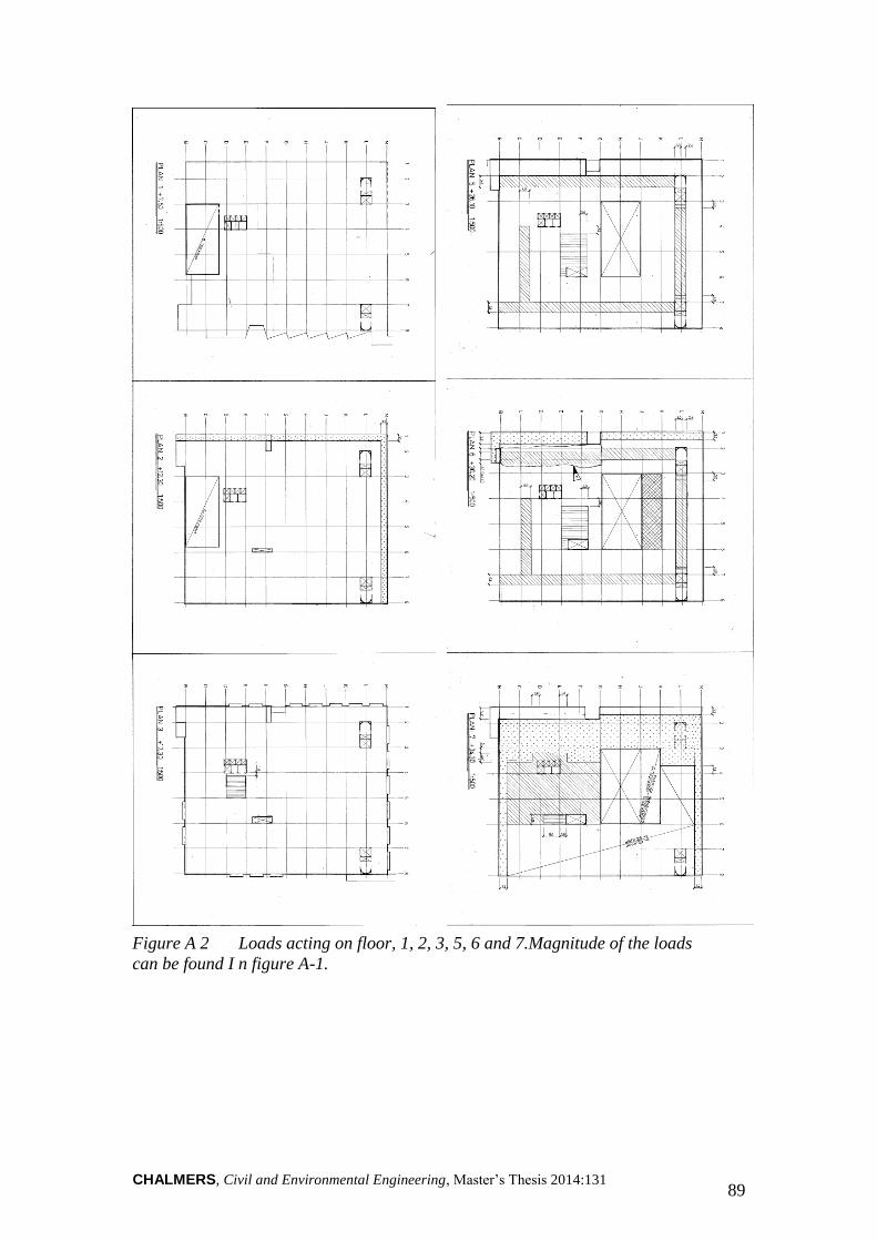
CHALMERS, Civil and Environmental Engineering, Master’s Thesis 2014:131 89
Figure A 2 Loads acting on floor, 1, 2, 3, 5, 6 and 7.Magnitude of the loads
can be found I n figure A-1.

CHALMERS, Civil and Environmental Engineering, Master’s Thesis 2014:131 90
Figure A 3 Construction drawing for location of the piles.

CHALMERS, Civil and Environmental Engineering, Master’s Thesis 2014:131 91
Appendix B – Hand calculations
Each colour represents a load, presented in the construction drawings above.
Figure B 1 Calculation of load acting on each pillar, based on construction
drawings in figures A1-A3.
q e
gq
nytt
[kP/m
2]
635400
Övrigt
q e
gq
nytt
[kP/m
2]
6352000
Plan
10
400-
815400
Plan
2815
400200
635500
Plan
3635
400-
1020800
Plan
4,5,6635
20070
1020550
1020400
1020400
635600
13700
D=D
eae
d w
eigh
t load
01200
W=W
orkin
g load
0
Tot D
[kP]
Tot W
[kP]To
t D [kP
]To
t W [kP
]Tot D
[kP]
Tot W
[kP]To
t D [kP
]To
t W [kP
]Tot D
[kP]
Tot W
[kP]To
t D [kP
]To
t W [kP
]To
t D [kP
]To
t W [kP
]Sn
ow
load
Are
a[m2]
Line
K
Pillar
Floo
r 1Flo
or 2
Floo
r 3Flo
or 4
Floo
r 5Flo
or 6
Floo
r 7R
oo
f
127,648
27,64827,648
27,64827,648
27,648
011059,2
28200,9611059,2
17556,4811059,2
17556,4811059,2
17556,485529,6
28200,9611059,2
241,472
1,15241,472
41,47241,472
3,072
57,640,32
57,657,6
51,8438,4
38,4
57,65,76
51,845,76
57,6
039628,8
80979,8439628,8
62910,7239628,8
62910,7239628,8
62910,7235366,4
64093,4435980,8
9792038400
3115,2
57,6115,2
115,257,6
57,657,6
28,8
57,663,36
34,5628,8
34,5628,8
23,04
046080
9388846080
7315246080
7315246080
76809,624192
90115,236288
123379,248384
0
4115,2
57,6115,2
115,263,36
34,5628,8
10,5623,04
57,663,36
34,5628,8
34,5618,24
23,04
34,5628,8
046080
9388846080
7315246080
7315246080
80467,225344
107078,449536
11114460096
0
5115,2
115,2115,2
57,628,8
28,834,56
28,834,56
28,823,04
50,47,2
34,5634,56
34,5628,8
34,5628,8
23,04
046080
9388846080
7315246080
11602846080
80467,225344
107078,449536
107078,462208
0
6115,2
115,2115,2
50,450,4
63,3634,56
28,834,56
28,823,04
7,27,2
57,657,6
57,623,04
28,8
046080
9388846080
7315246080
7574446080
76809,624192
90115,236288
90115,265664
0
7126,72
126,72126,72
50,460,48
57,657,6
126,7234,56
28,8
7,28,64
46,0846,08
34,5634,56
23,0423,04
050688
103276,850688
80467,250688
83318,450688
80467,239168
80467,239168
80467,276032
0
846,08
46,0846,08
40,3246,08
46,0846,08
14,414,4
5,76
018432
37555,218432
29260,818432
30297,618432
29260,89216
29260,89216
29260,827648
0
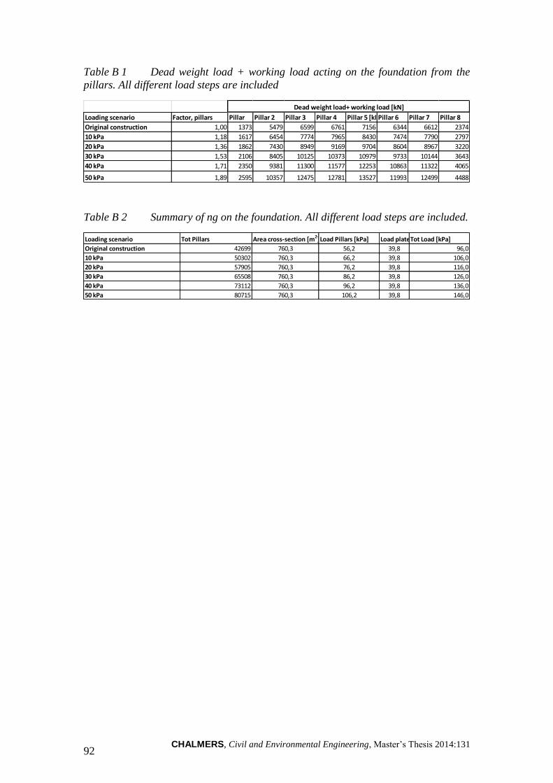
CHALMERS, Civil and Environmental Engineering, Master’s Thesis 2014:131 92
Table B 1 Dead weight load + working load acting on the foundation from the
pillars. All different load steps are included
Table B 2 Summary of ng on the foundation. All different load steps are included.
Loading scenario Factor, pillars Pillar Pillar 2 Pillar 3 Pillar 4 Pillar 5 [kN]Pillar 6 Pillar 7 Pillar 8
Original construction 1,00 1373 5479 6599 6761 7156 6344 6612 2374
10 kPa 1,18 1617 6454 7774 7965 8430 7474 7790 2797
20 kPa 1,36 1862 7430 8949 9169 9704 8604 8967 3220
30 kPa 1,53 2106 8405 10125 10373 10979 9733 10144 3643
40 kPa 1,71 2350 9381 11300 11577 12253 10863 11322 4065
50 kPa 1,89 2595 10357 12475 12781 13527 11993 12499 4488
Dead weight load+ working load [kN]
Loading scenario Tot Pillars Area cross-section [m2]Load Pillars [kPa] Load plate [kPa]Tot Load [kPa]
Original construction 42699 760,3 56,2 39,8 96,0
10 kPa 50302 760,3 66,2 39,8 106,0
20 kPa 57905 760,3 76,2 39,8 116,0
30 kPa 65508 760,3 86,2 39,8 126,0
40 kPa 73112 760,3 96,2 39,8 136,0
50 kPa 80715 760,3 106,2 39,8 146,0
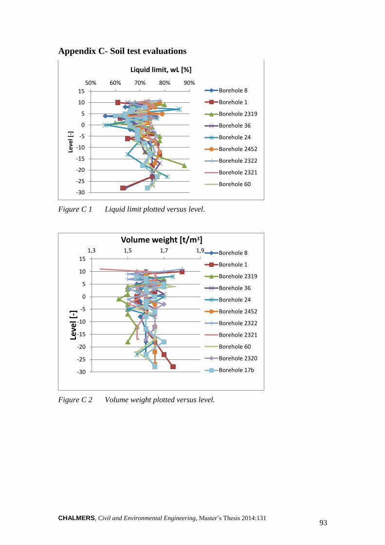
CHALMERS, Civil and Environmental Engineering, Master’s Thesis 2014:131 93
Appendix C- Soil test evaluations
Figure C 1 Liquid limit plotted versus level.
Figure C 2 Volume weight plotted versus level.
-30
-25
-20
-15
-10
-5
0
5
10
15
50% 60% 70% 80% 90%
Leve
l [-]
Liquid limit, wL [%]
Borehole 8
Borehole 1
Borehole 2319
Borehole 36
Borehole 24
Borehole 2452
Borehole 2322
Borehole 2321
Borehole 60
-30
-25
-20
-15
-10
-5
0
5
10
15
1,3 1,5 1,7 1,9
Leve
l [-]
Volume weight [t/m3]
Borehole 8
Borehole 1
Borehole 2319
Borehole 36
Borehole 24
Borehole 2452
Borehole 2322
Borehole 2321
Borehole 60
Borehole 2320
Borehole 17b
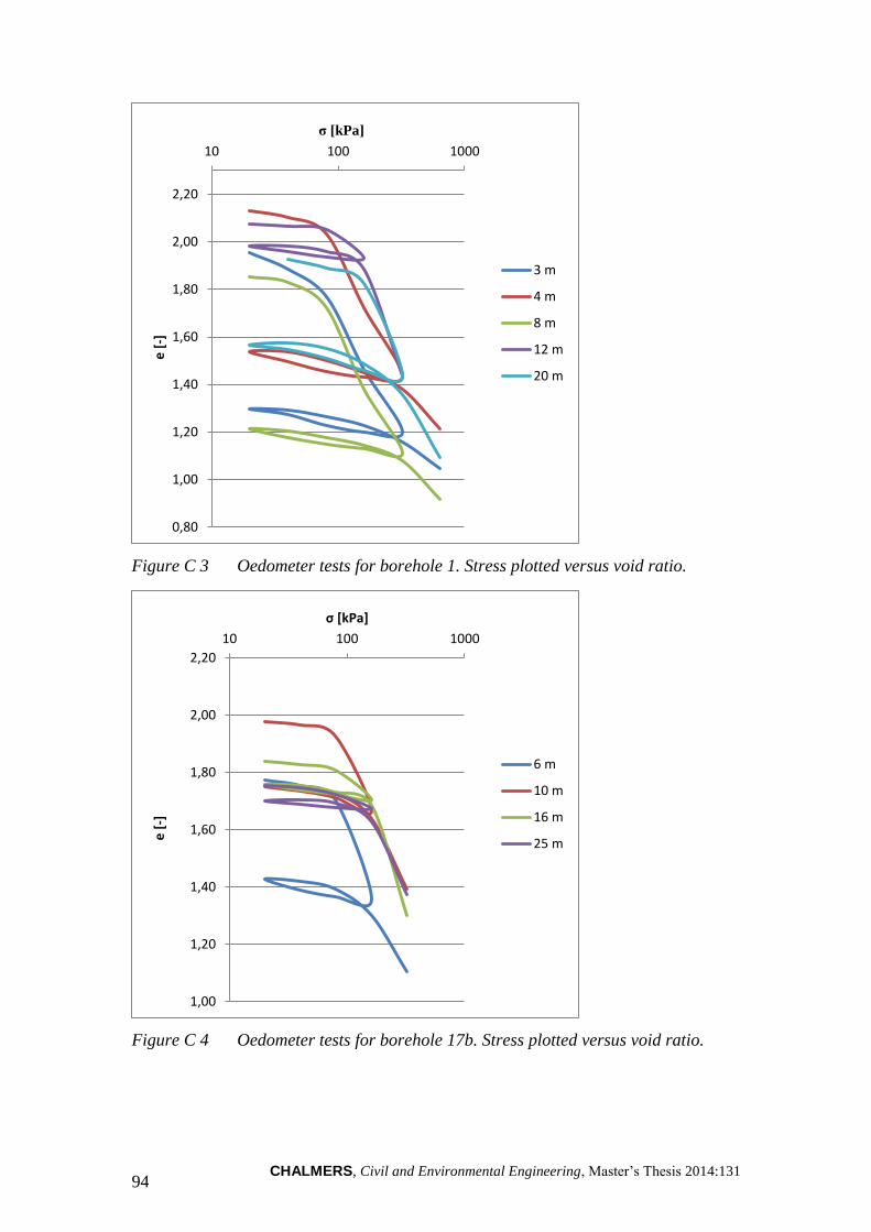
CHALMERS, Civil and Environmental Engineering, Master’s Thesis 2014:131 94
Figure C 3 Oedometer tests for borehole 1. Stress plotted versus void ratio.
Figure C 4 Oedometer tests for borehole 17b. Stress plotted versus void ratio.
0,80
1,00
1,20
1,40
1,60
1,80
2,00
2,20
10 100 1000 e
[-]
σ [kPa]
3 m
4 m
8 m
12 m
20 m
1,00
1,20
1,40
1,60
1,80
2,00
2,20
10 100 1000
e [
-]
σ [kPa]
6 m
10 m
16 m
25 m
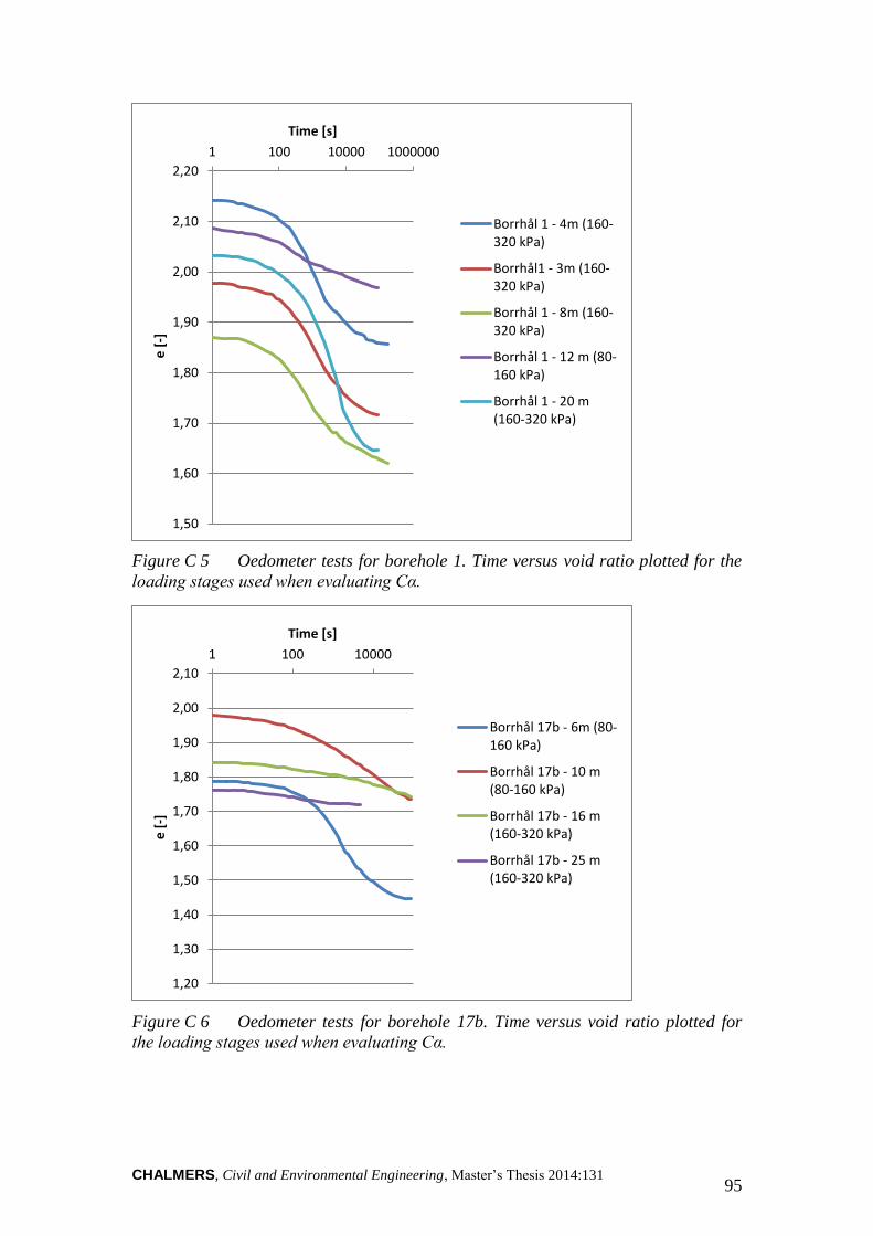
CHALMERS, Civil and Environmental Engineering, Master’s Thesis 2014:131 95
Figure C 5 Oedometer tests for borehole 1. Time versus void ratio plotted for the
loading stages used when evaluating Cα.
Figure C 6 Oedometer tests for borehole 17b. Time versus void ratio plotted for
the loading stages used when evaluating Cα.
1,50
1,60
1,70
1,80
1,90
2,00
2,10
2,20
1 100 10000 1000000 e
[-]
Time [s]
Borrhål 1 - 4m (160-320 kPa)
Borrhål1 - 3m (160-320 kPa)
Borrhål 1 - 8m (160-320 kPa)
Borrhål 1 - 12 m (80-160 kPa)
Borrhål 1 - 20 m(160-320 kPa)
1,20
1,30
1,40
1,50
1,60
1,70
1,80
1,90
2,00
2,10
1 100 10000
e [
-]
Time [s]
Borrhål 17b - 6m (80-160 kPa)
Borrhål 17b - 10 m(80-160 kPa)
Borrhål 17b - 16 m(160-320 kPa)
Borrhål 17b - 25 m(160-320 kPa)
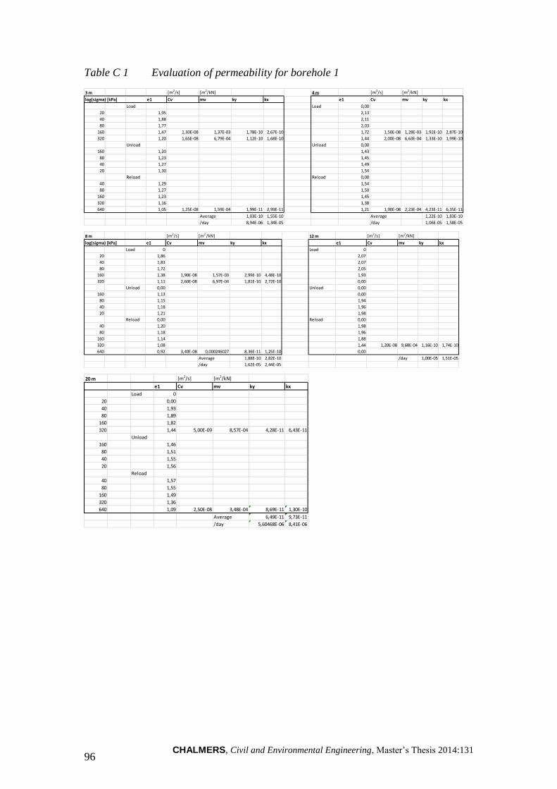
CHALMERS, Civil and Environmental Engineering, Master’s Thesis 2014:131 96
Table C 1 Evaluation of permeability for borehole 1
3 m [m2/s] [m2/kN] 4 m [m2/s] [m2/kN]
log(sigma) [kPa] e1 Cv mv ky kx e1 Cv mv ky kx
Load Load 0,00
20 1,95 2,13
40 1,88 2,11
80 1,77 2,03
160 1,47 1,30E-08 1,37E-03 1,78E-10 2,67E-10 1,72 1,50E-08 1,28E-03 1,91E-10 2,87E-10
320 1,20 1,65E-08 6,79E-04 1,12E-10 1,68E-10 1,44 2,00E-08 6,63E-04 1,33E-10 1,99E-10
Unload Unload 0,00
160 1,20 1,43
80 1,23 1,45
40 1,27 1,49
20 1,30 1,54
Reload Reload 0,00
40 1,29 1,54
80 1,27 1,50
160 1,23 1,45
320 1,16 1,38
640 1,05 1,25E-08 1,59E-04 1,99E-11 2,99E-11 1,21 1,90E-08 2,23E-04 4,23E-11 6,35E-11
Average 1,03E-10 1,55E-10 Average 1,22E-10 1,83E-10
/day 8,94E-06 1,34E-05 /day 1,06E-05 1,58E-05
8 m [m2/s] [m2 /kN] 12 m [m2/s] [m2/kN]
log(sigma) [kPa] e1 Cv mv ky kx e1 Cv mv ky kx
Load 0 Load 0
20 1,86 2,07
40 1,83 2,07
80 1,72 2,05
160 1,38 1,90E-08 1,57E-03 2,99E-10 4,48E-10 1,93
320 1,11 2,60E-08 6,97E-04 1,81E-10 2,72E-10 0,00
Unload 0,00 Unload 0,00
160 1,13 0,00
80 1,15 1,94
40 1,18 1,96
20 1,21 1,98
Reload 0,00 Reload 0,00
40 1,20 1,98
80 1,18 1,96
160 1,14 1,88
320 1,08 1,44 1,20E-08 9,68E-04 1,16E-10 1,74E-10
640 0,92 3,40E-08 0,000246027 8,36E-11 1,25E-10 0,00
Average 1,88E-10 2,82E-10 /day 1,00E-05 1,51E-05
/day 1,62E-05 2,44E-05
20 m [m2/s] [m2/kN]
e1 Cv mv ky kx
Load 0
20 0,00
40 1,93
80 1,89
160 1,82
320 1,44 5,00E-09 8,57E-04 4,28E-11 6,43E-11
Unload
160 1,46
80 1,51
40 1,55
20 1,56
Reload
40 1,57
80 1,55
160 1,49
320 1,36
640 1,09 2,50E-08 3,48E-04 8,69E-11 1,30E-10
Average 6,49E-11 9,73E-11
/day 5,60468E-06 8,41E-06
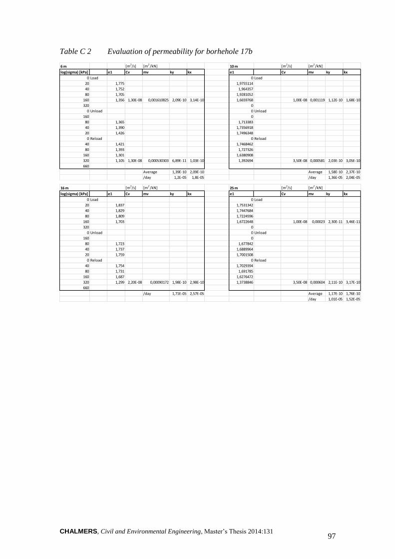
CHALMERS, Civil and Environmental Engineering, Master’s Thesis 2014:131 97
Table C 2 Evaluation of permeability for borhehole 17b
6 m [m2/s] [m2 /kN] 10 m [m2/s] [m2 /kN]
log(sigma) [kPa] e1 Cv mv ky kx e1 Cv mv ky kx
0 Load 0 Load
20 1,775 1,9755114
40 1,752 1,964357
80 1,705 1,9281052
160 1,356 1,30E-08 0,001610825 2,09E-10 3,14E-10 1,6659768 1,00E-08 0,001119 1,12E-10 1,68E-10
320 0
0 Unload 0 Unload
160 0
80 1,365 1,713383
40 1,390 1,7356918
20 1,426 1,7496348
0 Reload 0 Reload
40 1,421 1,7468462
80 1,393 1,727326
160 1,301 1,6380908
320 1,105 1,30E-08 0,000530303 6,89E-11 1,03E-10 1,392694 3,50E-08 0,000581 2,03E-10 3,05E-10
660
Average 1,39E-10 2,09E-10 Average 1,58E-10 2,37E-10
/day 1,2E-05 1,8E-05 /day 1,36E-05 2,04E-05
16 m [m2/s] [m2 /kN] 25 m [m2/s] [m2 /kN]
log(sigma) [kPa] e1 Cv mv ky kx e1 Cv mv ky kx
0 Load 0 Load
20 1,837 1,7531342
40 1,829 1,7447684
80 1,809 1,7224596
160 1,703 1,6722648 1,00E-08 0,00023 2,30E-11 3,46E-11
320 0
0 Unload 0 Unload
160 0
80 1,723 1,677842
40 1,737 1,6889964
20 1,759 1,7001508
0 Reload 0 Reload
40 1,754 1,7029394
80 1,731 1,691785
160 1,687 1,6276472
320 1,299 2,20E-08 0,00090172 1,98E-10 2,98E-10 1,3738846 3,50E-08 0,000604 2,11E-10 3,17E-10
660
/day 1,71E-05 2,57E-05 Average 1,17E-10 1,76E-10
/day 1,01E-05 1,52E-05

CHALMERS, Civil and Environmental Engineering, Master’s Thesis 2014:131 98
Table C 3 Hand calculated stress analysis
Table C 4 Hand calculations for design limits
Nivå Depth [m] z from y=5.8 σv [kPa] u [kPa] σ´o [kPa] σ´c [kPa] OCR KoOC KoNC σ´creep [kPa] σ´z Δσz σ´z+Δσz
12,1 0 0 0 0
10,1 2 36 0 36 0
9,1 3 52 10 42 80 1,90 0,69 0,5 64
8,1 4 68 20 48 90 1,88 0,68 0,5 72
6,1 6 100 40 60 84 1,40 0,59 0,5 67,2
5,8 6,3 0 104,8 43 61,8 75 1,21 0,55 0,5 60 0 53 53
4,1 8 1,7 132 60 72 82 1,14 0,53 0,5 65,6 10,2 51,0 61,2
2,1 10 3,7 164 80 84 94 1,12 0,53 0,5 75,2 22,2 48,8 71,0
0,1 12 5,7 196 100 96 110 1,15 0,54 0,5 88 34,2 46,7 80,9
-3,9 16 9,7 260 140 120 140 1,17 0,54 0,5 112 58,2 42,9 101,1
-7,9 20 13,7 324 180 144 170 1,18 0,54 0,5 136 82,2 39,5 121,7
γclay[kN/m3] 16 width [m] 79,2
γfill[kN/m3] 18 length [m] 96
q [kPa] 96
q' [kPa] 53 (load without uplifting water pressure)
Edge Middle
Length 1,5 2,4 [m]
Width 1,5 1,9 [m]
Area 2,25 4,56 [m2]
q_new_b 9,6 9,6 [MP/m2]
q_ground 5,1 5,1 [MP/m2]
q_pile 45,9 45,9 MP
q_water_now 3,9 3,8 [MP/m2]
q_water_org. Design 5 5 [MP/m2]
q_excavated 10,4 10,4 [MP/m2]
q_piles 20,4 10,1 [MP/m2]
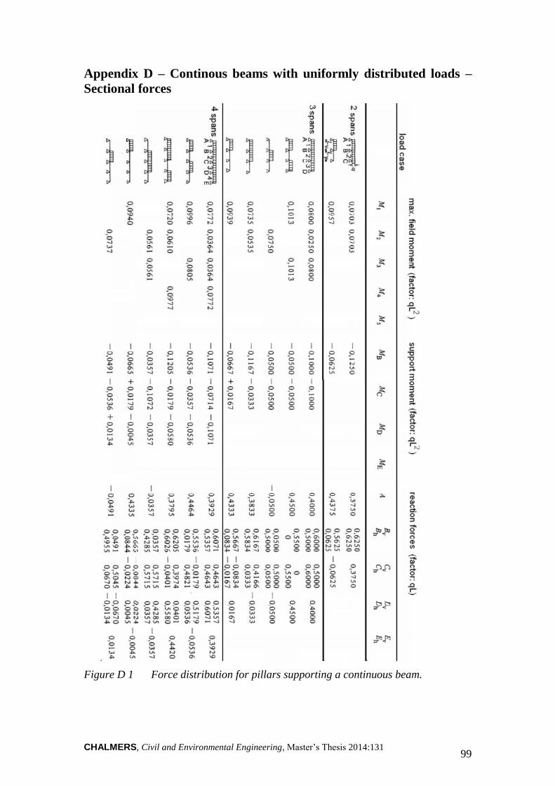
CHALMERS, Civil and Environmental Engineering, Master’s Thesis 2014:131 99
Appendix D – Continous beams with uniformly distributed loads –
Sectional forces
Figure D 1 Force distribution for pillars supporting a continuous beam.
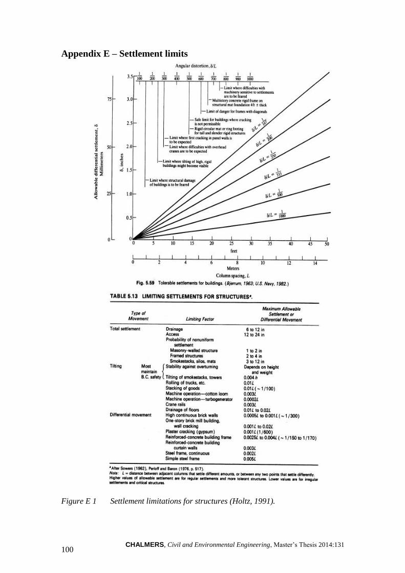
CHALMERS, Civil and Environmental Engineering, Master’s Thesis 2014:131 100
Appendix E – Settlement limits
Figure E 1 Settlement limitations for structures (Holtz, 1991).
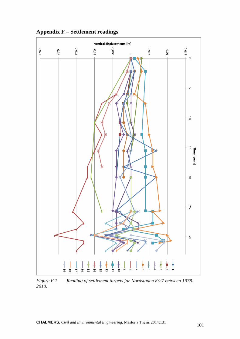
CHALMERS, Civil and Environmental Engineering, Master’s Thesis 2014:131 101
Appendix F – Settlement readings
Figure F 1 Reading of settlement targets for Nordstaden 8:27 between 1978-
2010.
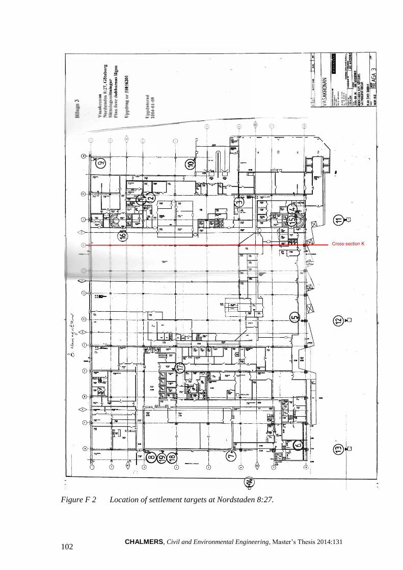
CHALMERS, Civil and Environmental Engineering, Master’s Thesis 2014:131 102
Figure F 2 Location of settlement targets at Nordstaden 8:27.