Modelling European regional FDI flows using a Bayesian ...

Vol.:(0123456789)

The Annals of Regional Science (2021) 67:593–616https://doi.org/10.1007/s00168-021-01058-x

1 3

ORIGINAL PAPER

Modelling European regional FDI flows using a Bayesian spatial Poisson interaction model

Tamás Krisztin1 · Philipp Piribauer2

Received: 28 October 2020 / Accepted: 17 March 2021 / Published online: 1 April 2021 © The Author(s) 2021

AbstractThis paper presents an empirical study of spatial origin and destination effects of European regional FDI dyads. Recent regional studies primarily focus on locational determinants, but ignore bilateral origin- and intervening factors, as well as associ-ated spatial dependence. This paper fills this gap by using observations on inter-regional FDI flows within a spatially augmented Poisson interaction model. We explicitly distinguish FDI activities between three different stages of the value chain. Our results provide important insights on drivers of regional FDI activities, both from origin and destination perspectives. We moreover show that spatial depend-ence plays a key role in both dimensions.

JEL Classification C11 · C21 · F23 · R11

1 Introduction

Recent decades have shown a rapid growth of worldwide foreign direct investment (FDI), which led to increased efforts in research to understand the economic deter-minants of FDI activities. Classical explanations focus on the factors driving firms to become multinational. The Ownership-Localization-Internalization theory (see Dunning 2001) explains firms’ motivation as an effort to internalize transaction costs and reap the benefits of externalities stemming from strategic assets.

A large alternative strand of empirical literature builds on trade theory. In this context the drivers of FDI activity are the need for larger sales markets, cheaper source markets, and the willingness to reach a technological frontier (Markusen 1995). Following empirical international economics literature, FDI flows are usually captured within the context of a bilateral spatial interaction model framework. The

* Tamás Krisztin [email protected]

1 International Institute for Applied Systems Analysis (IIASA), Schlossplatz 1, 2361 Laxenburg, Austria

2 Austrian Institute of Economic Research (WIFO), Arsenal 20, 1030 Vienna, Austria

http://orcid.org/0000-0002-9241-8628

http://crossmark.crossref.org/dialog/?doi=10.1007/s00168-021-01058-x&domain=pdf

594 T. Krisztin, P. Piribauer

1 3

main advantage of this approach is that it specifically accounts for the role of origin- and destination-specific factors, as well as intervening opportunities. For an over-view on the determinants of FDI activities and the location choice of multinationals, see Basile and Kayam (2015), Blonigen and Piger (2014), or Blonigen (2005).

Due to the scarcity of data on FDI activities on a subnational scale, the vast majority of the empirical literature focuses on country-specific FDI patterns. A sub-national perspective, however, would allow for in-depth decomposition of the spatial patterns of FDI flows, since FDI sources and destinations are not uniformly distrib-uted within a country, but tend to be spatially clustered. Multiple studies focusing on regional investment decisions of multinational companies (Crescenzi et al. 2013; Ascani et al. 2016a; Krisztin and Piribauer 2020) emphasize within-country hetero-geneity of FDI decisions, which can exceed cross-country differences. However, a major gap in the literature is that regional level studies only focus on the destina-tion of FDI decisions, and largely neglect to account for origin-specific factors, as well as intervening opportunities in a subnational context. However, a simultane-ous treatment appears particularly important for providing a complete picture on third-regional spatial interrelationships in both source- as well as destination-spe-cific characteristics (Leibrecht and Riedl 2014). Moreover, neglecting to take into account both origin, destination, and third region effects, can lead to biased param-eter estimates (Baltagi et al. 2007).

The present paper aims to fill these gaps by focusing on subnational FDI flows in a European multi-regional framework and explicitly accounting for origin-, des-tination-, as well as third region-specific factors. In this paper, we make use of sub-national data from the fDi Markets database, which reports on bilateral FDI flows, with detailed information on the source and destination city. This can be compiled to multiple dyadic format, that is each region pair appears twice, corresponding to FDI flowing from one region to the other and vice versa. A specific virtue of the database is that it distinguishes FDI flows by their respective business activity. This allows us to contrast the impact of origin, destination, and third region effects across multiple stages of the global values chain.

Origin- and destination-specific third region effects are captured in our empirical model in two ways. First, the model specification contains spatial contextual effects by means of spatially lagged explanatory variables (see Regelink and Elhorst 2015). Second, we moreover employ an econometric framework in the spirit of Koch and LeSage (2015) and LeSage et al. (2007) which captures spatial dependence using spatially-augmented random effects.

When adopting a subnational perspective, it is crucial to control for spatial dependence, as its presence in regional data is well documented (LeSage and Pace 2009). Even national-level empirical applications clearly document the presence of spatial spillovers on FDI activities. An influential example is the work by Bloni-gen et al. (2007), who analyse the determinants of US outbound FDI activities in a cross-country framework, while explicitly accounting for spatial dependence among destinations. Further studies which document the presence of spatial issues amongst bilateral (national) FDI activities include Pintar et al. (2016), Regelink and Elhorst (2015), Chou et al. (2011), Garretsen and Peeters (2009), Poelhekke and van der Ploeg (2009), or Baltagi et al. (2007).

595

1 3

Modelling European regional FDI flows using a Bayesian spatial…

We therefore employ a spatial augmented Bayesian Poisson specification on the pan-European subnational level which aims at dealing with both orgin- and destina-tion-specific characteristics. Estimation is achieved using work by Frühwirth-Schn-atter et al. (2009), allowing us to deal with high-dimensional specifications in a flex-ible and computationally efficient way.

The remainder of the paper is organized as follows. Section 2 presents the pro-posed spatial interaction model, which is augmented by spatial autoregressive ori-gin- and destination-specific random effects, intended to capture spatially depend-encies, as well as so-called third region effects. Section 3 details the FDI data, the considered determinants, as well as our selection of regions. In Sect. 4 we assess the determinants of European interregional FDI flows across different stages of the global value chain. The analysis is performed using information on FDI dyads cov-ering 266 NUTS-2 regions in the period 2003–2011. Section 5 concludes.

2 A spatial interaction model for subnational FDI flows

This section presents the model specification used for the empirical analysis. It is worth noting that the spatial econometric model is similar to work by LeSage et al. (2007), who aimed at modelling regional knowledge spillovers in Europe. An effi-cient Bayesian estimation approach for the employed multiplicative form of the Poisson model with spatial random effects is provided in the Appendix.1

Let y denote an N × 1 vector containing information on the number of FDI flows between n regions.2 In the classic spatial interaction model framework the flows are regressed on correspondingly stacked origin-, destination-, and distance-specific explanatory variables, as well as their spatially lagged counterparts. Xo and Xd denote N × pX origin- and destination-specific matrices of explanatory variables, respectively. Distances and further intervening factors between the n regions are captured by the N × pD matrix D.3 Extending the standard model specification with local spillover effects as well as spatial random effects, we consider a Poisson speci-fication of the form:

where P(⋅) denotes the Poisson distribution and �0 is an intercept parameter. �o , �d , and �D are parameter vectors corresponding to Xo , Xd , and D , respectively.

(2.1)

y ∼ P(�)

� = exp(�0 + Xo�o + Xd�d + D�D +WoXo�o +WdXd�d + Vo�o + Vd�d

),

1 Detailed R codes for running the proposed model are available upon request.2 It is worth noting that in the present study N is of lower dimension than n2 , since FDI dyads by con-struction exhibit no own-regional and no own-country flows.3 Detailed information on the straightforward construction of the origin- and destination-specific matri-ces of explanatory variables Xo and Xd from an n × pX dimensional matrix of explanatory variables is provided in LeSage and Pace (2009). LeSage and Pace (2009) also provide detailed guidelines on the convenient construction of origin- and destination-specific spatial weight matrices.


1 3

The spatial lags of the covariates are captured by WoXo and WdXd , with �o and �d denoting the respective pX × 1 vectors of parameters. Through these spatial lags we explicitly capture the so-called third region effects (Baltagi et al. 2007), that is ori-gin- and destination-specific spillovers from neighbouring regions. Neighbourhood effects are governed by non-negative, row-stochastic spatial weight matrices, which contain information on the spatial connectivity between the regions under scru-tiny. Our Poisson spatial interaction model includes separate spatial weight matri-ces Wo and Wd to account for origin- and destination-specific third regional effects, respectively.

Origin-based random effects are captured by the term Vo�o , where Vo denotes an N × n matrix of origin-specific dummy variables with a corresponding n × 1 vector �o . Similarly, the n × 1 vector �d captures regional effects associated with the des-tination regions’ matrix of dummy variables Vd . We follow work by LeSage et al. (2007) and introduce a further source of spatial dependence via the n × 1 regional effect vectors �o and �d , which are assumed to follow a first-order spatial autoregres-sive process:

where �o and �d denote origin- and destination-specific spatial autoregressive (sca-lar) parameters, respectively. W denotes an n × n row-stochastic spatial weight matrix with known constants and zeros on the main diagonal.

The disturbance error vectors �o and �d are both assumed to be independently and identically normally distributed, with zero mean and �2

o and �2

d variance,

respectively. Note that this assumption implies a one-to-one mapping to origin- and destination-specific normally distributed random effects in the case of �o = 0 and �d = 0 . For a row-stochastic W , a sufficient stability condition may be employed by assuming the spatial autoregressive parameters �o and �d to lie in the interval −1 < 𝜌o, 𝜌d < 1 (see, for example, LeSage and Pace 2009).

3 Bilateral FDI data and regions

Our data set comprises observations on regional FDI dyads for 266 European NUTS-2 regions in the period 2003–2011. A complete list of the regions in our sam-ple is provided in Table 6 in the Appendix.

Observations on regional cross-border greenfield FDI investments stem from the fDi Markets database. This database is maintained by fDi Intelligence, which is a specialist division of the Financial Times Ltd. The provided data draws on media and corporate sources to report on the sources and hosts of FDI flows (detailed by country, region, and city), industry classifications, as well as the level of capi-tal investment. Crescenzi et al. (2013) report several robustness tests and detailed comparisons with official data sources. They confirm the reliability of the fDi

(2.2)�o = �oW�o + �o�o = N(0,�2

oIn)

(2.3)�d = �dW�d + �d�d = N(0,�2

dIn),

597

1 3


Markets data set, especially with regard to the reported spatial distribution of FDI investments.

Our dependent variables are based on the total amount of inflows from European regions in the period 2003 to 2011. Since the fDi Markets data base also contains information on several distinct business activities for both origin and host compa-nies, we follow previous studies by Ascani et al. (2016a) and study the determinants of regional FDI dyads at different stages of the value chain. This information is valu-able as investor companies maximize their utility with respect to their position along the value chain. Since specifics of the investor company, as well as details on the FDI investment are largely unobserved, it is crucial to account for the heterogene-ity in investor decisions by subdividing industry activities relative to their position along the value chain (see, for example, Ascani et al. 2016a). We therefore define three different classifications: Upstream, Downstream, and Production. The classi-fication adopted in this paper builds on general classifications of the value chain by Sturgeon (2008) and closely tracks the ones employed by Crescenzi et al. (2013) and Ascani et al. (2016a).

Specifically, the upstream category comprises conceptual product development including design and testing, as well as management and business administration activities. The downstream category summarizes consumer-related activities such as sales, product delivery, or support. Finally, the production category includes activi-ties related to physical product creation, including extraction, manufacturing, as well as recycling activities. A complete list of the employed global value chain classifica-tion is provided in Table 5 in the Appendix.

Our choices for explanatory variables are motivated by recent literature on (regional) FDI flows as well as regional growth empirics (see, for example, Cre-spo Cuaresma et al. 2018; Blonigen and Piger 2014; Leibrecht and Riedl 2014; or Blonigen 2005). In most gravity-type models, a region’s ability to emit and attract FDI flows is chiefly captured by its economic characteristics. Our main indicator for economic characteristics is the regions’ market size, proxied by regional gross value added. To control for the degree of urbanization both in origin and host regions, we also include regional population densities as an additional covariate. Empirical evidence suggests (Coughlin et al. 1991; Huber et al. 2017) that higher wages have a deterrent effect on investment. We proxy this in our model by including the average compensation of employees per hour worked as an explanatory variable.

We account for the regional industry mix by including the share of employment in manufacturing and construction (NACE classifications B to F), as well as ser-vices (NACE G to U). We moreover include typical supply-side quantities such as regional endowments of human and knowledge capital. To proxy regional human capital endowments, we include two different variables. The first variable measures regional tertiary education attainment shares labelled higher education workers. A second variable labelled lower education workers is proxied by the share of the working age population with lower secondary education levels or less.

We use data on patent numbers to proxy regional knowledge capital endowments. Patent data exhibit particularly desirable characteristics for this purpose, since they can be viewed as a direct result of research and development activities (LeSage and Fischer 2012). In order to construct regional knowledge stocks, we use the perpetual


1 3

inventory method. We follow Fischer and LeSage (2015) and LeSage and Fischer (2012) to construct knowledge capital stocks Kit for region i in period t. Specifically, we define Kit = (1 − rK)Kit−1 + Pit , where rK = 0.10 denotes a constant depreciation rate and Pit denotes the number of patent applications in region i at time t.

The matrix D includes several different distance metrics. First and foremost, we include the geodesic distance between parent and host regions. Recent empirical lit-erature also consider common language as a potential quantity in D (see Krisztin and Fischer 2015, or Blonigen and Piger 2014). We measure whether the same offi-cial language is present in the source and host regions through a dummy variable. Information on official national and minority languages is obtained from the Euro-pean Commission.

Several studies on FDI flows also highlight the importance of corporate tax rates as a potential key quantity to attract FDI inflows (see Blonigen and Piger 2014; Leibrecht and Riedl 2014; Bellak and Leibrecht 2009). Lower corporate income tax rates in the host region as compared to the origin region are thus expected to increase the potential attractiveness of FDI inflows. Matrix D therefore also contains the (country-specific) difference in corporate income tax rates between origin and destination regions. Larger differences are expected to be associated with increasing FDI inflows.

In order to alleviate potential endogeneity problems, we moreover measure all explanatory variables at the beginning of our sample (that is in 2003).4 For speci-fication of the spatial weight matrix, we rely on a row-stochastic seven nearest neighbour specification.5 Data on the variables used stem from the fDi Markets, Cambridge Econometrics, as well as the Eurostat regional databases. Detailed infor-mation on the construction of the dependent and explanatory variables used are pre-sented in Table 1.

4 Empirical results

This subsection presents the empirical results obtained from 15,000 posterior draws after discarding the first 10,000 as burn-ins. Running multiple chains with alternat-ing starting values did not affect the empirical results, which also provides evidence for sampler convergence.

Posterior quantities for upstream-, downstream-, and production-related invest-ment flows are presented in Tables 2, 3, and 4, respectively. Each table reports poste-rior means and posterior standard deviations for the quantities of interest. Statistical significance of the respective posterior mean estimates is based on a 90% credible interval and highlighted in bold. The first block in each table presents origin- and

4 To assess the robustness of the results we also estimated a model where the explanatory variables were averages from 2003 to 2011. Overall the estimated quantities and their statistical significance remained unchanged.5 A series of tests using different number of nearest neighbours for the neighbourhood structure appeared to affect the results in a negligible way.

599

1 3


Tabl

e 1

Var

iabl

es u

sed

in th

e em

piric

al il

lustr

atio

n

ISC

ED a

nd N

AC

E re

fer t

o th

e in

tern

atio

nal s

tand

ard

clas

sific

atio

n of

edu

catio

n an

d th

e se

cond

revi

sion

of t

he s

tatis

tical

cla

ssifi

catio

n of

eco

nom

ic a

ctiv

ities

in th

e Eu

ro-

pean

com

mun

ity, r

espe

ctiv

ely

Varia

ble

Des

crip

tion

yU

pstre

amFD

I infl

ows a

ssoc

iate

d w

ith u

pstre

am a

ctiv

ities

. Sou

rce:

fDi M

arke

tsD

owns

tream

FDI i

nflow

s ass

ocia

ted

with

dow

nstre

am a

ctiv

ities

. Sou

rce:

fDi M

arke

tsPr

oduc

tion

FDI i

nflow

s ass

ocia

ted

with

pro

duct

ion

activ

ities

. Sou

rce:

fDi M

arke

tsX

Mar

ket s

ize

Prox

ied

by m

eans

of r

egio

nal g

ross

val

ue a

dded

, in

log

term

s. So

urce

: Cam

brid

ge E

cono

met

rics

Popu

latio

n de

nsity

Popu

latio

n pe

r squ

are

km, i

n lo

g te

rms.

Sour

ce: C

ambr

idge

Eco

nom

etri

csC

ompe

nsat

ion

per h

our

Com

pens

atio

n of

em

ploy

ees p

er h

ours

wor

ked,

in lo

g te

rms.

Sour

ce: C

ambr

idge

Eco

nom

etri

csEm

ploy

men

t in

indu

stry

Shar

e of

NA

CE

B to

F (i

ndus

try a

nd c

onstr

uctio

n) in

tota

l em

ploy

men

t. So

urce

: Cam

brid

ge E

cono

met

-ri

csEm

ploy

men

t in

serv

ices

Shar

e of

NA

CE

G to

U (s

ervi

ces)

in to

tal e

mpl

oym

ent.

Sour

ce: C

ambr

idge

Eco

nom

etri

csLo

wer

edu

catio

n w

orke

rsSh

are

of p

opul

atio

n (a

ged

25 a

nd o

ver)

with

low

er e

duca

tion

(ISC

ED le

vels

0-2

). So

urce

: Eur

osta

tH

ighe

r edu

catio

n w

orke

rsSh

are

of p

opul

atio

n (a

ged

25 a

nd o

ver)

with

hig

her e

duca

tion

(ISC

ED le

vels

6+

). So

urce

: Eur

osta

tRe

gion

al k

now

ledg

e ca

pita

lK

now

ledg

e sto

ck fo

rmat

ion

mea

sure

d in

term

s of p

aten

t acc

umul

atio

n, in

log

term

s. So

urce

: Eur

osta

tD

Geo

grap

hic

dist

ance

Geo

desi

c di

stan

ce b

etw

een

sour

ce a

nd h

ost r

egio

n. S

ourc

e: E

uros

tat

Diff

eren

ce in

tax

rate

sC

ount

ry-s

peci

fic to

p st

atut

ory

corp

orat

e in

com

e ta

x ra

tes (

incl

udin

g su

rcha

rges

). M

easu

red

by m

eans

of

diffe

renc

e be

twee

n so

urce

and

hos

t reg

ion.

Sou

rce:

Eur

osta

tC

omm

on la

ngua

geD

umm

y va

riabl

e, 1

den

otes

that

the

regi

ons s

hare

a c

omm

on o

ffici

al la

ngua

ge, 0

oth

erw

ise.

Sou

rce:

Eu

rope

an C

omm

issi

on


1 3

destination-specific slope parameter estimates, respectively. These estimates are reported for both own region characteristics as well as their spatial lags or third region characteristics (Baltagi et al. 2007). In the spatial econometrics literature, the former are often referred to as average direct impacts. Third region effects cap-tured by spatially lagged counterparts are typically referred to as average indirect (or spillover) impacts (LeSage and Pace 2009). The second block in each table reports posterior summary metrics for the spatial autoregressive origin and destination ran-dom effects. The third and last block in each table shows posterior inference for the variables used in the distance matrix D.

4.1 Origin‑ and destination‑specific core variables

Table 2 reports posterior parameter estimates for upstream FDI (most notably consisting of business services and headquarters). Starting with the key drivers for regions producing FDI outflows in upstream-related activities, Table 2 shows

Table 2 Posterior parameter estimates for FDI associated with upstream value chains.

The model includes a constant. Results based on 15,000 Markov-chain Monte Carlo iterations, where the first 10,000 were discarded as burn-in. Estimates in bold are statistically significant under a 90% confi-dence interval

Variable Origin Destination

Mean Std. Dev. Mean Std. Dev.

Market size 1.26 0.12 1.32 0.07Population density 0.33 0.12 0.29 0.04Compensation per hour −0.59 0.31 −0.94 0.17Employment in industry −1.93 1.31 −0.03 0.75Employment in services 2.02 1.86 2.08 0.83Lower education workers −0.01 1.05 −1.03 0.81Higher education workers 3.86 0.66 4.14 0.78Regional knowledge capital 0.08 0.03 −0.02 0.05W Market size −2.04 0.18 −0.53 0.10W Population density −0.47 0.10 −0.35 0.06W Compensation per hour −0.14 0.26 −0.63 0.27W Employment in industry −2.04 1.83 0.20 1.31W Employment in services 1.47 1.57 −2.79 1.54W Lower education workers 0.42 0.93 -0.01 1.01W Higher education workers 2.18 1.01 2.44 0.94W Regional knowledge capital −0.94 0.17 0.20 0.10�o , �

d0.58 0.08 0.44 0.09

�2

o , �2

d0.70 0.08 1.28 0.13

Geographic distance −1.01 0.03Difference in tax rates 1.30 0.63Common language 0.51 0.07

601

1 3


particularly strong evidence for the importance of the own-regional market size and population density. In addition, the corresponding third-regional effects are significant and negative. For example, an increase in the market size restricted only to neighbouring regions thus decreases the amount of FDI outflows from a given region. The table also suggests a particularly accentuated importance of a well educated working age population (higher education workers) in the ori-gin region. The estimated impact appears much more pronounced as compared to downstream and production FDI. Moreover, for upstream FDI the third region effect associated with the higher education workers variable also appears to be positive and highly significant. Own-regional knowledge capital endowments appear to be positively associated with the generation of upstream FDI outflows. However, the impacts of regional knowledge capital endowments for upstream FDI outflows appear rather muted as compared to the other types of FDI consid-ered. Interestingly, Table 2 shows negative third-regional impacts for knowledge capital. Unlike other types of FDI under scrutiny, the compensation per hour

Table 3 Posterior parameter estimates for FDI associated with downstream value chains.




Market size 0.65 0.10 1.26 0.06Population density 0.24 0.08 0.17 0.05Compensation per hour −0.43 0.33 −0.92 0.17Employment in industry −1.33 0.98 2.38 1.10Employment in services 0.61 1.13 2.97 0.69Lower education workers −1.03 0.74 −1.10 0.64Higher education workers 2.90 0.64 3.29 0.89Regional knowledge capital 0.38 0.05 −0.06 0.03W Market size −1.34 0.11 −0.55 0.15W Population density −0.63 0.19 −0.13 0.09W Compensation per hour −0.58 0.21 −0.48 0.20W Employment in industry −2.14 1.13 0.92 0.93W Employment in services −1.15 1.68 −1.31 0.98W Lower education workers 1.01 1.01 1.53 0.68W Higher education workers 1.78 1.04 1.24 0.94W Regional knowledge capital −0.92 0.17 0.26 0.10�o , �

d0.42 0.12 0.52 0.08

�2

o , �2

d0.39 0.05 0.75 0.09



1 3

variable only appears to have a significant impact for own-regional upstream FDI outflows.

Inspection of the regional determinants to attract upstream FDI inflows shows some interesting similarities to the origin-specific characteristics. This holds par-ticularly true for the market size and population density variables. Both desti-nation-specific variables show a positive and highly significant own-regional impact, with negative (and significant) spatial lags. Similar to the origin spe-cific determinants of upstream FDI, the corresponding host-specific impacts appear more pronounced as in other activity types. This finding is in line with Henderson and Ono (2008), Defever (2006), or Duranton and Puga (2005), who highlight that the location choice of business services and headquarters related activities are particularly driven by functional aspects (rather than by sectoral aspects) and typically tend to be located in urban agglomerations. Regional FDI inflows associated with upstream investment activities moreover appear to be par-ticularly attracted by regions with a higher specialization in the services sector

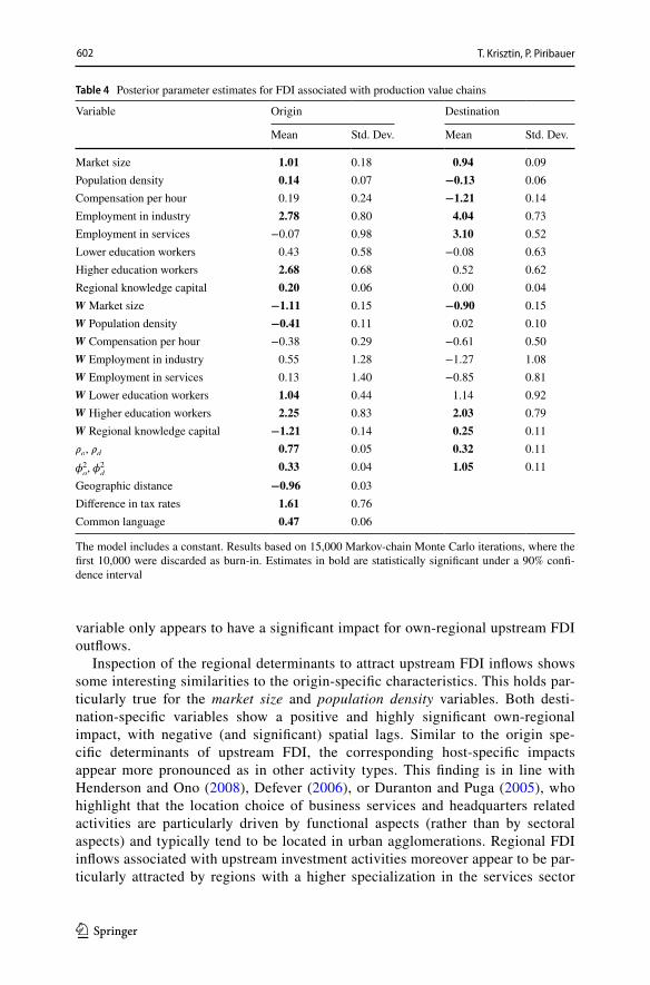
Table 4 Posterior parameter estimates for FDI associated with production value chains




Market size 1.01 0.18 0.94 0.09Population density 0.14 0.07 −0.13 0.06Compensation per hour 0.19 0.24 −1.21 0.14Employment in industry 2.78 0.80 4.04 0.73Employment in services −0.07 0.98 3.10 0.52Lower education workers 0.43 0.58 −0.08 0.63Higher education workers 2.68 0.68 0.52 0.62Regional knowledge capital 0.20 0.06 0.00 0.04W Market size −1.11 0.15 −0.90 0.15W Population density −0.41 0.11 0.02 0.10W Compensation per hour −0.38 0.29 −0.61 0.50W Employment in industry 0.55 1.28 −1.27 1.08W Employment in services 0.13 1.40 −0.85 0.81W Lower education workers 1.04 0.44 1.14 0.92W Higher education workers 2.25 0.83 2.03 0.79W Regional knowledge capital −1.21 0.14 0.25 0.11�o , �

d0.77 0.05 0.32 0.11

�2

o , �2

d0.33 0.04 1.05 0.11


603

1 3


(employment in services), relative to the agriculture sector (which serves as the benchmark in the specifications).

From a theoretical point of view, we would also expect labour costs, measured in terms of compensation per hours, to be an important determinant for attracting FDI inflows. This hypothesis is confirmed by inspecting the destination-specific results across all tables. Significant negative direct impacts of this variable can be observed throughout all stages of the value chain, both concerning the own region, as well as third regions. This corroborates the findings of Ascani et al. (2016b), who study the location determinants of Italian multinational enterprises. Regional knowledge capi-tal as a pull-factor for upstream FDI inflows appears less relevant. Only the respec-tive third-regional impact is significant, however, it appears comparatively muted.

Overall, the results for downstream FDI reported in Table 3 show a strong simi-larity to those of upstream FDI (Table 2). This resemblance can be observed for both origin- and destination-specific spatial determinants. For regions as a source of downstream FDI, Table 3 also highlights the key importance of agglomeration forces, proxied by the variables market size and population density. Both variables show a positive and significant direct impact for the generation of downstream FDI outflows, along with negative third-regional effects. These impacts, however, appear somewhat less pronounced as compared to upstream FDI. Similarly, the impact of regional tertiary education attainment (higher education workers) for downstream FDI outflows appears less accentuated as compared to upstream FDI outflows. As opposed to the results for origin-specific upstream FDIs, the third-regional effects of tertiary education attainment are insignificant. Regional knowledge capital endow-ments, on the other hand, appear somewhat more important for generating down-stream FDI as compared to upstream FDI, with positive direct, and negative third-regional effects.

In line with the prevalent literature (see, among others, Leibrecht and Riedl 2014; Casi and Resmini 2010; or Baltagi et al. 2007), the destination-specific regional determinants for downstream FDI also show a strong importance of the market size and population density variables as a means to attracting downstream-related FDI inflows. Similar to destination-specific upstream FDI, educational attainment (lower and higher education workers) and the compensation per hour variable appear as important pull-factors. Concerning the regional industry mix, Table 3 suggests that higher shares in the industry and service sectors (employment in industry and services) appear to be significantly and positively associated with attracting down-stream-related FDI inflows. An interesting result is given by a negative and statis-tically significant own-regional impact of the regional knowledge capital variable. The estimated impacts, however, appear rather offset by the positive third-regional impacts. Similar results can also be found in work by Dimitropoulou et al. (2013), a study on the location determinants of FDI for UK regions.

Empirical results for production-related FDI are summarized in Table 4. Starting with the origin-specific determinants of generating production FDI outflows, Table 4 shows not surprisingly a pronounced importance of regional market size and popula-tion density. Similar to the other types of FDI, both variables also exhibit significant negative third-regional effects. Interestingly, the source regional industry mix also appears to play a key role. Specifically, the employment in industry variable shows


1 3

a positive and highly significant direct impact of the origin region. The remaining origin-specific drivers are basically in line with those of the other types of FDI, most notably positive impacts of tertiary education attainment (higher education workers) levels and regional knowledge capital endowments.

Inspection of the destination-specific determinants of production-related FDI, however, reveals markedly different patterns as compared to upstream and down-stream FDI. Albeit the market size shows a similar importance, along with nega-tive third-regional effects, the direct impact of the population density variable shows a negative and significant sign. Our estimation results thus show that production-oriented FDI activities are predominantly attracted by smaller regions in proxim-ity to urban agglomerations. For upstream and downstream activities, however, urban agglomerations seem to play a more central role. Moreover, our results imply that regional human capital endowments are particularly important for explaining upstream and downstream-oriented investment decisions. For production activities, the importance of regional human capital endowments appears slightly less pro-nounced. These results corroborate the findings of Strauss-Kahn and Vives (2009), and Defever (2006) by highlighting that industry-related location decisions typically focus on sectoral, rather than on functional aspects. The significant and positive own-regional, destination-specific industry mix (employment in industry and ser-vices) further underpins these findings.

For attracting production-related FDI, Table 4 shows a particularly pronounced negative impact of the compensation per hour variable of the host region. The neg-ative direct impact on inflows is the strongest with a posterior mean of −1.21 for production-related activities. However, it is worth noting that the associated third-regional impacts on inflows are insignificant for production, whereas both down-stream and upstream related FDI flows exhibit significant negative third-regional impacts. Our findings are moreover in line with Fallon and Cook (2014) and Cres-cenzi et al. (2013), who both find that locational drivers for production-related FDI flows differ from those associated with business service activities.

4.2 Spatial‑dependence and distance metrics

This subsection discusses the results for the spatial autoregressive origin and des-tination random effects, as well as the estimates of intervening opportunities from the distance matrix D . Inspection of posterior estimates for the spatial latent random effects provides significant evidence for pronounced spatial dependence patterns in the random effects across all stages of the value chain. This finding holds true for both source- and host-regional heterogeneity in the sample. Posterior estimates for spatially structured origin- and destination-specific random effects for upstream, downstream and production stages of the value chain are illustrated in Fig. 1. Ori-gin-specific effects are depicted in the top row, while destination-specific effects are in the bottom. Positive values are shaded in red, while negative values are shaded in blue. Regions which were not significant under a 95% posterior credible interval are shaded in white.

605

1 3


A comparison of their corresponding posterior means and standard deviations shows that all spatial autoregressive parameters are estimated with a high preci-sion. The intensity of spatial dependence in the upstream- and downstream-spe-cific latent unobservable effects appear similarly pronounced, with values rang-ing from 0.42 to 0.58. For production-related investment activities, the difference between �o and �d appears more pronounced, with the former being particularly sizeable (0.77), while the latter appears more muted.

Rather similar results for upstream, downstream and production are also reported for the distance factors collected in matrix D . As expected, the poste-rior mean estimates for geographical distance are negative and significantly differ from zero for all types of investment activities. Moreover, the posterior standard deviations are comparatively small, indicating that the impact of geographic dis-tance is estimated with a high precision. Higher geographic separation of two regions is thus associated with lower FDI activities, as increased distance often raises transportation, monitoring and thus investment costs. The negative impacts

Fig. 1 Spatially structured origin- and destination-specific random effects across the value chain. Notes Regions that are not statistically significant under 95% credible intervals are shaded in white


1 3

reported in Tables 2, 3, and 4 are in line with recent empirical results in FDI (Lei-brecht and Riedl 2014) and trade literature (Krisztin and Fischer 2015).

Our dummy variable measuring whether a pair of regions shares an official common language proxies the cultural distance between regions in the sample. As expected, the reported posterior means show a positive sign and are significantly dif-ferent from zero. The third distance variable in the matrix D measures the (country-specific) difference in corporate tax rates between source and target regions. In line with theoretical and empirical literature on the location choice of multinationals, the tables report significant and positive impacts to regional FDI flows when corporate tax rates in the target region are lower than in the source region (see Bellak and Leibrecht 2009 and Strauss-Kahn and Vives 2009). The estimated posterior means for the difference in tax rates suggest that a 1% decrease in the tax rate difference between source and destination regions results in a 1.3% and 3.5% increase in the number of FDI flows for downstream and upstream related activities, respectively.

5 Conclusions

This paper presents an empirical study on the spatial determinants of bilateral FDI flows among European regions. Due to data scarcity on the subnational level, previous papers typically adopt a national perspective when analysing FDI dyads (see, for example, Leibrecht and Riedl 2014). This paper thus provides a first spa-tial econometric analysis on the European regional level by explicitly accounting for origin-, destination-, and third region-specific factors in the analysis. The sub-national perspective of our analysis allows us to study the spatial spillover mecha-nisms of regional FDI flows in more detail. Unlike recent studies on the locational determinants of FDI inflows (see, for example, Ascani et al. 2016b; or Crescenzi et al. 2013), we model FDI decision determinants not only across destination regions but also across the origin regional dimension. Moreover, due to the well-known need to control for spatial dependence when modelling regional data (LeSage and Pace 2009), we also capture spatial dependence through spatially structured random effects associated with origin and destination regions.

Our data comes from the fDi Markets database, which contains detailed infor-mation on regional FDI activities using media sources and company data. The data from the fDi Markets database also contains detailed sectoral information on the functional form of the FDI activity, which allows us to explicitly focus on FDI flows across different stages of the value chain. Specifically, the paper studies the origin- and destination-specific determinants of upstream, downstream, and production activities.

Our empirical results clearly indicate that both source and destination spatial dependence plays a key role for all investment activities under scrutiny. In line with recent literature, we find that regional market size, corporate tax rates, as well as third region effects appear to be of particular importance for all stages in the value chain. We moreover find that production-oriented FDI activities are predominantly attracted by smaller regions in proximity to urban agglomerations. For upstream and downstream activities, however, being in the same region as urban agglomerations

607

1 3


seem to play a key role. Moreover, our results imply that regional human capital endowments are particularly important for explaining upstream and downstream-oriented investment decisions. For production activities, the importance of regional human capital endowments are less accentuated. These results corroborate the findings of Strauss-Kahn and Vives (2009), or Defever (2006) by highlighting that industry-related location decisions typically focus on sectoral, rather than on func-tional aspects. From an origin-specific perspective of FDI activities, our empirical results moreover clearly show that regional knowledge capital endowments appear crucial for host regions to produce FDI outflows. Similar to the results on the desti-nation-specific factors for FDI inflows, we also find high education and agglomera-tion forces as particularly important aspects for host regional FDI outflows.

Appendix

Detailed description of the Bayesian Markov‑chain Monte Carlo algorithm

This section provides a detailed description of the employed Bayesian Markov-chain Monte Carlo (MCMC) algorithm. A similar version is employed by LeSage et al. (2007), who use such a modelling strategy for estimation of knowledge spillovers (measured in terms of patenting dyads) in European regions. Specifically, their esti-mation approach relies on work by Frühwirth-Schnatter and Wagner (2006), who introduce a Bayesian auxiliary mixture sampling approach for non-Gaussian distrib-uted data. This approach builds on a hierarchical data augmentation procedure by introducing yi + 1 latent variables for each observation yi , where yi denotes the i-th element of y (with i = 1, ...,N).

In order to alleviate the implied computational burden, we rely on an improved version of this auxiliary mixture sampling algorithm (Frühwirth-Schnatter et al. 2013). The algorithm tremendously reduces the number of latent parameters per observation. Specifically, the required number of latent parameters is reduced from yi + 1 to at most two per observation for Poisson distributed data (Frühwirth-Schnat-ter et al. 2013).

From a statistical point of view, �i from Eq. (2.1) can be interpreted as a param-eter in a Poisson process describing occurring events in a given time interval, where �i denotes the i-th element of the Poisson mean � . For illustration, imagine sorting all unique values of the observed FDI flows from lowest to highest. The Poisson pro-cess can be viewed as modelling – given a specific number of FDI flows – the prob-ability of jumping from one unique value to the next. These two quantities can be characterized as so-called arrival and inter-arrival times. Motivated by this formula-tion, the distribution itself can be described using merely arrival and inter-arrival times, derived from the rate of the process �i . The expected value of arrival time of yi is 1∕�i and it follows a Gamma distribution with shape one and rate equal to yi . The inter-arrival times are by definition independent and arise from an exponential distribution with rate equal to �i . Based on this definition, we can model �i if we


1 3

sample from the inter-arrival time �i1 between yi and yi + 1 , as well as for yi > 0 , the arrival �i2 time for yi . The main contribution of Frühwirth-Schnatter et al. (2009) is that they introduce auxiliary variables for �i1 and �i2 , conditional on yi.

For this purpose let us define the latent variables �i1 and �i2 , based on the proper-ties of arrival and inter-arrival times:

, where E(⋅) denotes the exponential and G(⋅, ⋅) the Gamma distribution. The arrival times �i2 only apply for yi > 0 , since zero values have by definition no arrival time. Eqs. (A.1) and (A.2) can be log-linearized in the following fashion:

(A.1)�i1 =�i1

�i, �i1 ∼ E(1)

(A.2)𝜏i2 =𝜉i2

𝜆i, 𝜉i1 ∼ G(yi, 1) ∀ yi > 0,

(A.3)− ln �i1 = ln �i + �i1, �i1 = − ln �i1

Table 5 Classification of fDi Markets business functions

The last column indicates the percent of industry activities per FDI classification. The values are based on the total observed FDI flows in the fDi Markets database targeting the selected NUTS-2 regions in the period 2003-2011

Classification Business activities % of classifi-cation

Upstream Business Services 64.0Design, Development and Testing 10.8Education and Training 2.5Headquarters 12.1Information and Communication Tech-

nology and Internet Infrastructure4.3

Research and Development 6.3Downstream Customer Contact Centre 4.2

Logistics, Distribution and Transportation 26.9Maintenance and Servicing 3.4Sales, Marketing and Support 62.1Shared Services Centre 2.0Technical Support Centre 1.4

Production Construction 21.0Electricity 5.3Extraction 0.3Manufacturing 72.1Recycling 1.3

609

1 3


Tabl

e 6

List

of r

egio

ns in

the

study

Aus

tria

Fran

ce [c

ontin

ued]

Hun

gary

Pola

nd [c

ontin

ued]

UK

Bur

genl

and

(AT)

Lang

uedo

c-Ro

ussi

llon

Dél

-Alfö

ldLó

dzki

eB

edfo

rdsh

ire a

nd H

ertfo

rdsh

ireK

ärnt

enLi

mou

sin

Dél

-Dun

ántú

lLu

bels

kie

Ber

kshi

re, B

ucki

ngha

msh

ire a

ndN

iede

röste

rrei

chLo

rrai

neÉs

zak-

Alfö

ldLu

busk

ie

Oxf

ords

hire

Obe

röste

rrei

chM

idi-P

yrén

ées

Észa

k-M

agya

rors

zág

Mal

opol

skie

Che

shire

Salz

burg

Nor

d - P

as-d

e-C

alai

sK

özép

-Dun

ántú

lM

azow

ieck

ieC

ornw

all a

nd Is

les o

f Sci

llySt

eier

mar

kPa

ys d

e la

Loi

reK

özép

-Mag

yaro

rszá

gO

pols

kie

Cum

bria

Tiro

lPi

card

ieN

yuga

t-Dun

ántú

lPo

dkar

pack

ieD

erby

shire

and

Not

tingh

amsh

ireVo

rarlb

erg

Poito

u-C

hare

ntes

Irel

and

Podl

aski

eD

evon

Wie

nPr

oven

ce-A

lpes

-Côt

e d’

Azu

rB

orde

r, M

idla

nd a

nd W

este

rnPo

mor

skie

Dor

set a

nd S

omer

set

Belg

ium

Rhô

ne-A

lpes

Sout

hern

and

Eas

tern

Slas

kie

East

Ang

liaPr

ov. A

ntw

erpe

nG

erm

any

Ital

ySw

ieto

krzy

skie

East

Wal

esPr

ov. B

raba

nt W

allo

nA

rnsb

erg

Abr

uzzo

War

min

sko-

Maz

ursk

ieEa

st Yo

rksh

ire a

ndPr

ov. H

aina

utB

erlin

Bas

ilica

taW

ielk

opol

skie

N

orth

ern

Linc

olns

hire

Prov

. Liè

geB

rand

enbu

rgC

alab

riaZa

chod

niop

omor

skie

Easte

rn S

cotla

ndPr

ov. L

imbu

rg (B

E)B

raun

schw

eig

Cam

pani

aPo

rtug

alEs

sex

Prov

. Lux

embo

urg

(BE)

Bre

men

Emili

a-Ro

mag

naA

lent

ejo

Glo

uces

ters

hire

, Wilt

shire

and

Prov

. Nam

urC

hem

nitz

Friu

li-Ve

nezi

a G

iulia

Alg

arve

B

risto

lPr

ov. O

ost-V

laan

dere

nD

arm

stad

tLa

zio

Àre

a M

etro

polit

ana

de L

isbo

aG

reat

er M

anch

este

rPr

ov. V

laam

s-B

raba

ntD

etm

old

Ligu

riaC

entro

(PT)

Ham

pshi

re a

nd Is

le o

f Wig

htPr

ov. W

est-V

laan

dere

nD

resd

enLo

mba

rdia

Nor

teH

eref

ords

hire

, Wor

ceste

rshi

reRé

gion

de

Bru

xelle

s-C

apita

leD

üsse

ldor

fM

arch

eR

oman

ia

and

War

wic

kshi

reBu

lgar

iaFr

eibu

rgM

olis

eB

ucur

esti

- Ilfo

vH

ighl

ands

and

Isla

nds

Seve

ren

tsen

trale

nG

ieße

nPi

emon

teC

entru

Inne

r Lon

don

Seve

roiz

toch

enH

ambu

rgPr

ovin

cia

Aut

onom

a di

Bol

zano

/N

ord-

Est

Ken

tSe

vero

zapa

den

Han

nove

r

Boz

enN

ord-

Vest

Lanc

ashi

reY

ugoi

ztoc

hen

Kar

lsru

hePr

ovin

cia

Aut

onom

a di

Tre

nto

Sud

- Mun

teni

aLe

ices

ters

hire

, Rut

land

and


1 3

Tabl

e 6

(con

tinue

d)

Aus

tria

Fran

ce [c

ontin

ued]

Hun

gary

Pola

nd [c

ontin

ued]

UK

Yug

ozap

aden

Kas

sel

Pugl

iaSu

d-Es

t

Nor

tham

pton

shire

Yuz

hen

tsen

trale

nK

oble

nzSa

rdeg

naSu

d-Ve

st O

lteni

aLi

ncol

nshi

reC

zech

Rep

ublic

Köl

nSi

cilia

Vest

Mer

seys

ide

Jihov

ýcho

dLe

ipzi

gTo

scan

aSl

ovak

iaN

orth

Eas

tern

Sco

tland

Jihoz

ápad

Lüne

burg

Um

bria

Bra

tisla

vský

kra

jN

orth

Yor

kshi

reM

orav

skos

lezs

koM

eckl

enbu

rg-V

orpo

mm

ern

Valle

d’A

osta

/Val

lée

d’A

oste

Stre

dné

Slov

ensk

oN

orth

ern

Irel

and

(UK

)Pr

aha

Mitt

elfr

anke

nVe

neto

Výc

hodn

é Sl

oven

sko

Nor

thum

berla

nd a

nd T

yne

and

Seve

rový

chod

Mün

ster

Latv

iaZá

padn

é Sl

oven

sko

W

ear

Seve

rozá

pad

Nie

derb

ayer

nLa

tvija

Slov

enia

Out

er L

ondo

nSt

redn

í Cec

hyO

berb

ayer

nLi

thua

nia

Vzh

odna

Slo

veni

jaSh

rops

hire

and

Sta

fford

shire

Stre

dní M

orav

aO

berf

rank

enLi

etuv

aZa

hodn

a Sl

oven

ijaSo

uth

Wes

tern

Sco

tland

Den

mar

kO

berp

falz

Luxe

mbu

rgSw

eden

Sout

h Yo

rksh

ireH

oved

stad

enR

hein

hess

en-P

falz

Luxe

mbu

rgM

elle

rsta

Nor

rland

Surr

ey, E

ast a

nd W

est S

usse

xM

idtjy

lland

Saar

land

Net

herl

ands

Nor

ra M

ella

nsve

rige

Tees

Val

ley

and

Dur

ham

Nor

djyl

land

Sach

sen-

Anh

alt

Dre

nthe

Östr

a M

ella

nsve

rige

Wes

t Mid

land

sSj

ælla

ndSc

hles

wig

-Hol

stein

Flev

olan

dÖ

vre

Nor

rland

Wes

t Wal

es a

nd T

he V

alle

ysSy

ddan

mar

kSc

hwab

enFr

iesl

and

(NL)

Smål

and

med

öar

naW

est Y

orks

hire

Esto

nia

Stut

tgar

tG

elde

rland

Stoc

khol

mEe

stiTh

ürin

gen

Gro

ning

enSy

dsve

rige

Finl

and

Trie

rLi

mbu

rg (N

L)V

ästs

verig

eÅ

land

Tübi

ngen

Noo

rd-B

raba

ntSp

ain

Etel

ä-Su

omi

Unt

erfr

anke

nN

oord

-Hol

land

And

aluc

íaH

elsi

nki-U

usim

aaW

eser

-Em

sO

verij

ssel

Ara

gón

Läns

i-Suo

mi

Gre

ece

Utre

cht

Can

tabr

ia

611

1 3


Tabl

e 6

(con

tinue

d)

Aus

tria

Fran

ce [c

ontin

ued]

Hun

gary

Pola

nd [c

ontin

ued]

UK

Pohj

ois-

ja It

ä -S

uom

iA

nato

liki M

aked

onia

, Thr

aki

Zeel

and

Cas

tilla

y L

eón

Fran

ceA

ttiki

Zuid

-Hol

land

Cas

tilla

-la M

anch

aA

lsac

eD

ytik

i Ella

daN

orw

ayC

atal

uña

Aqu

itain

eD

ytik

i Mak

edon

iaA

gder

og

Roga

land

Com

unid

ad d

e M

adrid

Auv

ergn

eIo

nia

Nis

iaH

edm

ark

og O

ppla

ndC

omun

idad

For

al d

e N

avar

raB

asse

-Nor

man

die

Ipei

ros

Nor

d-N

orge

Com

unid

ad V

alen

cian

aB

ourg

ogne

Ken

triki

Mak

edon

iaO

slo

og A

kers

hus

Extre

mad

ura

Bre

tagn

eK

riti

Sør-Ø

stlan

det

Gal

icia

Cen

tre (F

R)

Not

io A

igai

oTr

ønde

lag

Illes

Bal

ears

Cha

mpa

gne-

Ard

enne

Pelo

ponn

isos

Vestl

ande

tLa

Rio

jaC

orsi

caSt

erea

Ella

daPo

land

País

Vas

coFr

anch

e-C

omté

Thes

salia

Dol

nosl

aski

ePr

inci

pado

de

Astu

rias

Hau

te-N

orm

andi

eVo

reio

Aig

aio

Kuj

awsk

o-Po

mor

skie

Regi

ón d

e M

urci

aÎle

de

Fran

ce

The

not-b

old

parts

are

the

subn

atio

nal r

egio

ns b

elon

ging

to a

cou

ntry

, whi

le th

e bo

lded

par

ts a

re c

ount

ry n

ames


1 3

, where for yi = 0 only Eq. (A.3) is defined. Evidently, if �i1 and �i2 would be Gauss-ian this would imply a linear model, which could be easily sampled from. While �i1 and �i2 are not Gaussian per se, the distributions can be approximated by a mix-ture of Gaussians, from which sampling can easily be achieved (Frühwirth-Schnatter et al. 2009).

In order to obtain a model which is conditionally Gaussian, the non-normal density can be approximated by a mixture of Q(�) normal components, where � denotes the shape parameter of a Gamma distribution. For sampling �i1 we can set � = 1 , and in the case of sampling �i1 the rate � would be equal to yi . There-fore, the mixture of normal components can be generalised for both distribu-tions. Thus, the mixture distribution is given by the following:

where wq(�) denotes the weight, mq(�) the mean, and sq(�) the variance. These components, as well as Q(�) directly depend on the choice of � . Values for all these parameters conditional on � are provided in Frühwirth-Schnatter et al. (2009). To approximate the Poisson process through the Gaussian mixture in Eq. (A.5), the additional latent discrete variable �i1 , and additionally in cases of yi > 0 the discrete variable �i2 are introduced.

Given �i1 and �i1 and additionally for the case of yi > 0 �i2 and �i2 , the condi-tional posterior of the Poisson model’s slope parameters are Gaussian:

We can easily sample from the distributions given in Eqs. (A.6) and (A.7) and there-fore construct an efficient Gibbs sampling algorithm (for a detailed description, see Section 1 in the Appendix).

For Bayesian estimation, we have to define prior distributions for all param-eters in the model. We follow the canonical approach and use a Gaussian prior setup for the parameters �0 , �o , �d , �D , �o , and �d with zero mean and a rela-tively large prior variance of 104 . We follow LeSage et al. (2007) in our choice of priors for the spatially structured random effect vectors and set a normal prior structure �o and �d , with with zero mean and �2

x

(AxAx

)−1 variance, where x ∈ [o, d] and Ax = In − �xW . For the variance of the random effects �2

x we

employ an inverse Gamma prior with rate equal to 5 and the shape parameter to 0.05. Following LeSage et al. (2007), we elicit a non-informative uniform prior specification �x ∼ U(−1, 1).

(A.4)− ln 𝜏i2 = ln 𝜆i + 𝜀i2, 𝜀i2 = − ln 𝜉i2 ∀ yi > 0,

(A.5)p�(�|�) ∼Q(�)∑

q=1

wq(�)N[�|mq(�), sq(�)

],

(A.6)− ln �i1 = ln �i + m(1) + �i1, �i1|�i1 ∼ N[0, s(1)]

(A.7)− ln 𝜏i2 = ln 𝜆i + m(𝜈i2) + 𝜀i2, 𝜀i2|𝜈i2 ∼ N[0, s(𝜈i2)

]∀ yi > 0.

613

1 3


The Gibbs sampling scheme

Let us collect the explanatory variables from Eq. (2.1) in an N × P (with P = 1 + 4pX + pD ) matrix Z = [�N ,Xo,Xd,D,WoXo,WdXd] and � = [�0, �

�o, ��

d, ��

D, ��

o, ��

d]� . Thus, � = exp

(Z� + Vo�o + Vd�d

).

Moreover, let us denote the number of non-zero observations in y as Ny>0 . Then, let N+ = N + Ny>0 and let the N+ × 1 vector y+ be y+ = [y�, y�

y>0]� , where yy>0 con-

tains all elements of y which are greater than zero. Moreover, let the N+ × P matrix Z+ be Z+ = [Z�,Z�

y>0]� , where the matrix Zy>0 contains all rows of Z corresponding

to yk > 0 . In a similar fashion, we augment the dummy observation matrices Vo and Vd and denote the resulting N+ × n matrices as V+

o and V+

d.

Accordingly we order the auxiliary variables corresponding to �i1 and �i2 and col-lect them into the following N+ × 1 auxiliary variable vectors as � = [𝜏11, ..., 𝜏N1, 𝜏12, ..., 𝜏Ny>02

] and � = [𝜈11, ..., 𝜈N1, 𝜈12, ..., 𝜈Ny>02] . Based on this, we

define the N+ × N+ variance matrix � . Additionally – based on the definition of the Gaussian mixtures in Eqs. (A.6, A.7) – an N+ × 1 vector of working responses y can be obtained conditional on � and � , so that y = m(�) − ln �.

Given appropriate starting values the following Gibbs sampling algorithm can be devised:

I. Sample � from its conditional Gaussian distribution p(�|⋅) ∼ N(�� ,��) , where

�� denotes the P × P prior variance matrix and �

� the P × 1 matrix of prior

means. II. Sample �x from their conditional distributions p(�x|⋅) ∼ N(��x

��x,��x

) , where

III. We sample �2x from the conditional posterior, which is inverse Gamma distrib-

uted and given as p(�2x|⋅) ∼ IG(sx, 1∕vx) , where

sx and v

x denote the prior rate and shape parameters of the inverse gamma

distribution IG(⋅, ⋅). IV. For �x the conditional posterior distribution is:

Unfortunately, this is not a well-known distribution, thus – as is standard in the spatial econometric literature – we resort to a griddy Gibbs step (Ritter

�� =(Z�+�

−1Z+ + �−1�

)−1

�� = Z�+�

−1(y − V+o�o − V+

d�d) + �

−1��.

��x=(𝜙−2xAx

�Ax + V+�

x�

−1V+x

)−1

��x= V+�

x�

−1(y − Z+� − V+

x�x

).

sx = (n + sx)∕2vx =

(��xA�xAx�x + s

xvx

)∕2.

p(�x|⋅) ∝ |Ax| exp(−

1

2�2x

��xA�xAx�x

).


1 3

and Tanner 1992) in order to sample from the conditional posterior for �x.6 For this purpose candidate values �∗

x are sampled from �∗

x= N(�x,��x ) , where

��x is the proposal density variance, which is adaptively adjusted using the

procedure from LeSage and Pace (2009) and thus is constrained to a desired interval by the means of rejection sampling. The candidate values are evalu-ated using their full posterior distributions7.

V. For i = 1, ...,N we sample �i1 from �i1 ∼ Ex(�i) and set �i1 = 1 + �i1 . If yk > 0 then we additionally sample �i2 from B(yi, 1) (where B(⋅) denotes the Beta distribution) and set �i1 = 1 − �i2 + �i1.

VI. For i = 1, ...,N we sample �i1 from the discrete distribution involving the mix-ture of normal distributions with r = 1, ...,Q(1) :

and for yi > 1 we additionally sample �i2 from the discrete distribution (with r = 1, ...,Q(yi) ):

With the sampled values for � and � , we update y = ln � − m(�) and �.This concludes the Gibbs sampling algorithm. The Markov-chain Monte Carlo algo-rithm cycles through steps I. to VI. B times and excludes the initial B0 draws as burn-ins. Inference regarding the parameters is subsequently conducted using the remaining B − B0 draws.8

Acknowledgements The research carried out in this paper was supported by funds of the Oesterreichische Nationalbank (Jubilaeumsfond project number: 18116), and of the Austrian Science Fund (FWF): ZK 35.

Funding Open access funding provided by International Institute for Applied Systems Analysis (IIASA).

Open Access This article is licensed under a Creative Commons Attribution 4.0 International License, which permits use, sharing, adaptation, distribution and reproduction in any medium or format, as long as you give appropriate credit to the original author(s) and the source, provide a link to the Creative Com-mons licence, and indicate if changes were made. The images or other third party material in this article are included in the article’s Creative Commons licence, unless indicated otherwise in a credit line to the material. If material is not included in the article’s Creative Commons licence and your intended use is not permitted by statutory regulation or exceeds the permitted use, you will need to obtain permission directly from the copyright holder. To view a copy of this licence, visit http:// creat iveco mmons. org/ licen ses/ by/4. 0/.

p(�i1 = r|⋅) ∝ wr(1)N[− ln �i1 − ln �i|mr(1), sr(1)

]

p(�i2 = r|⋅) ∝ wr(yi)N[− ln �i2 − ln �i|mr(yi), sr(yi)

].

8 Whether the MCMC algorithm converged can be easily verified using convergence diagnostics by Geweke (1991) or Raftery and Lewis (1992). For the present application we utilised an implementation of these convergence diagnostics from the R coda package.

6 An alternative, however, computationally more intensive approach also frequently used in the spatial econometric literature involves a Metropolis-Hastings step for the spatial autoregressive parameter (see, for example, LeSage and Pace 2009).7 In practice it is costly to evaluate the log-determinant directly. Instead we use an adapted version of the log-determinant approximation by Pace and Barry (1997) for pre-calculation.

http://creativecommons.org/licenses/by/4.0/

http://creativecommons.org/licenses/by/4.0/

615

1 3


References

Ascani A, Crescenzi R, Iammarino S (2016a) Economic institutions and the location strategies of Euro-pean multinationals in their geographic neighborhood. Econ Geogr 92(4):401–429

Ascani A, Crescenzi R, Iammarino S (2016b) What drives European multinationals to the European Union neighbouring countries? A mixed-methods analysis of Italian investment strategies. Environ Plan C: Gov Policy 34(4):656–675

Baltagi BH, Egger P, Pfaffermayr M (2007) Estimating models of complex FDI: are there third-country effects? J Econom 140(1):260–281

Basile R, Kayam S (2015) Empirical literature on location choice of multinationals. In: Commendatore P, Kayam S, Kubin I (eds) Complexity and geographical economics. Springer, Cham, pp 325–351

Bellak C, Leibrecht M (2009) Do low corporate income tax rates attract FDI? Evidence from Central- and East European countries. Appl Econ 41(21):2691–2703

Blonigen BA (2005) A review of the empirical literature on FDI determinants. Atl Econ J 33(4):383–403Blonigen BA, Davies RB, Waddell GR, Naughton HT (2007) FDI in space: spatial autoregressive rela-

tionships in foreign direct investment. Eur Econ Rev 51(5):1303–1325Blonigen BA, Piger J (2014) Determinants of foreign direct investment. Can J Econ 47(3):775–812Casi L, Resmini L (2010) Evidence on the determinants of foreign direct investment: the case of EU

regions. East J Eur Stud 1(2):93–118Chou KH, Chen CH, Mai CC (2011) The impact of third-country effects and economic integration on

China’s outward FDI. Econ Model 28(5):2154–2163Coughlin CC, Terza JV, Arromdee V (1991) State characteristics and the location of foreign direct invest-

ment within the United States. Revi Econ Stat 73(4):675–683Crescenzi R, Pietrobelli C, Rabellotti R (2013) Innovation drivers, value chains and the geography of

multinational corporations in Europe. J Econ Geogr 14(6):1053–1086Crespo Cuaresma J, Doppelhofer G, Huber F, Piribauer P (2018) Human capital accumulation and long-

term income growth projections for European regions. J Reg Sci 58(1):81–99Defever F (2006) Functional fragmentation and the location of multinational firms in the enlarged

Europe. Reg Sci Urban Econ 36(5):658–677Dimitropoulou D, McCann P, Burke SP (2013) The determinants of the location of foreign direct invest-

ment in UK regions. Appl Econ 45(27):3853–3862Dunning JH (2001) The eclectic (OLI) paradigm of international production: past, present and future. Int

J Econ Bus 8(2):173–190Duranton G, Puga D (2005) From sectoral to functional urban specialisation. J Urban Econ 57(2):343–370Fallon G, Cook M (2014) Explaining manufacturing and non-manufacturing inbound FDI location in five

UK regions. Tijdschrift voor Economische en Sociale Geografie 105(3):331–348Fischer MM, LeSage JP (2015) A Bayesian space-time approach to identifying and interpreting regional

convergence clubs in Europe. Pap Reg Sci 94(4):677–702Frühwirth-Schnatter S, Frühwirth R, Held L, Rue H (2009) Improved auxiliary mixture sampling for

hierarchical models of non-Gaussian data. Stat Comput 19(4):479–492Frühwirth-Schnatter S, Halla M, Posekany A, Pruckner G and Schober T (2013) Applying standard and

semiparametric Bayesian IV on health economic data. In: Bayesian Young statisticians meeting (BAYSM). pp. 1–4

Frühwirth-Schnatter S, Wagner H (2006) Auxiliary mixture sampling for parameter-driven models of time series of counts with applications to state space modelling. Biometrika 93(4):827–841

Garretsen H, Peeters J (2009) FDI and the relevance of spatial linkages: do third-country effects matter for Dutch FDI? Rev World Econ 145(2):319–338

Geweke J (1991) Evaluating the accuracy of sampling-based approaches to the calculation of posterior moments, vol 196. Federal Reserve Bank of Minneapolis, Research Department Minneapolis, MN, USA

Henderson JV, Ono Y (2008) Where do manufacturing firms locate their headquarters? J Urban Econ 63(2):431–450

Huber F, Fischer MM, Piribauer P (2017) The role of US based FDI flows for global output dynamics. Macroecon Dyn 23(3):943–973

Koch W, LeSage JP (2015) Latent multilateral trade resistance indices: theory and evidence. Scott J Pol Econ 62(3):264–290


1 3

Krisztin T, Fischer MM (2015) The gravity model for international trade: specification and estimation issues. Sp Econ Anal 10(4):451–470

Krisztin T, Piribauer P (2020) A Bayesian spatial autoregressive logit model with an empirical appli-cation to European regional FDI flows. Empir Econ (forthcoming). https:// doi. org/ 10. 1007/ s00181- 020- 01856-w

Leibrecht M, Riedl A (2014) Modeling FDI based on a spatially augmented gravity model: evidence for Central and Eastern European Countries. J Int Trade Econ Dev 23(8):1206–1237

LeSage JP, Fischer MM (2012) Estimates of the impact of static and dynamic knowledge spillovers on regional factor productivity. Int Reg Sci Rev 35(1):103–127

LeSage JP, Fischer MM, Scherngell T (2007) Knowledge spillovers across Europe: evidence from a Pois-son spatial interaction model with spatial effects. Pap Reg Sci 86(3):393–421

LeSage JP, Pace RK (2009) Introduction to spatial econometrics. CRC Press, Boca RatonMarkusen JR (1995) The boundaries of multinational enterprises and the theory of international trade. J

Econ Perspect 9(2):169–189Pace RK, Barry RP (1997) Quick computation of regressions with a spatially autoregressive dependent

variable. Geogr Anal 29(3):291–297Pintar N, Sargant B, Fischer MM (2016) Austrian outbound foreign direct investment in Europe: a spatial

econometric study. Roman J Reg Sci 10(1):1–22Poelhekke S, van der Ploeg F (2009) Foreign direct investment and urban concentrations: unbundling

spatial lags. J Reg Sci 49(4):749–775Raftery AE, Lewis S (1992) How many iterations in the Gibbs sampler? In: Bernardo JM, Berger J,

Dawid AP, Smith AFM (eds) Bayesian statistics 4. Oxford University Press, Oxford, pp 763–773Regelink M, Elhorst JP (2015) The spatial econometrics of FDI and third country effects. Lett Sp Resour

Sci 8(1):1–13Ritter C, Tanner MA (1992) Facilitating the Gibbs sampler: the Gibbs stopper and the griddy-Gibbs sam-

pler. J Am Stat Assoc 87(419):861–868Strauss-Kahn V, Vives X (2009) Why and where do headquarters move? Reg Sci Urban Econ

39(2):168–186Sturgeon TJ (2008) Mapping integrative trade: conceptualising and measuring global value chains. Int J

Technol Learn, Innov Dev 1(3):237–257

Publisher’s Note Springer Nature remains neutral with regard to jurisdictional claims in published maps and institutional affiliations.

https://doi.org/10.1007/s00181-020-01856-w

https://doi.org/10.1007/s00181-020-01856-w

Modelling European regional FDI flows using a Bayesian ...

Documents

Transcript of Modelling European regional FDI flows using a Bayesian ...