Modelling and Forecasting financial time series of«tick data» by functional analysis and neural

networks

S. DABLEMONT, S. VAN BELLEGEM, M. VERLEYSEN

Université catholique de Louvain, Machine Learning Group, DICE3, Place du Levant, B-1348 Louvain-la-Neuve - BELGIUM

Tel : +32 10 47 25 51 - Fax : +32 10 47 25 98E-mail : {dablemont, verleysen}@dice.ucl.ac.be

vanbellegem@stat.ucl.ac.be

SubjectsFinances , Neural Networks, Forecasting, Nonlinear Time Series Models, Tick Data

AbstractThe analysis of financial time series is of primary importance in the economic world.

This paper deals with a data-driven empirical analysis of financial time series. The goalis to obtain insights into the dynamics of series and out-of-sample forecasting.

In this paper we present a forecasting method based on an empirical functional anal-ysis of the past of series.

An originality of this method is that it does not make the assumption that a singlemodel is able to capture the dynamics of the whole series. On the contrary, it splitsthe past of the series into clusters, and generates a specific local neural model for eachof them. The local models are then combined in a probabilistic way, according to thedistribution of the series in the past.

This forecasting method can be applied to any time series forecasting problem, but isparticularly suited for data showing nonlinear dependencies, cluster effects and observedat irregularly and randomly spaced times like high-frequency financial time series do. Oneway to overcome the irregular and random sampling of "tick-data" is to resample themat low-frequency, as it is done with "Intraday". However, even with optimal resamplingusing say five minute returns when transactions are recorded every second, a vast amountof data is discarded, in contradiction to basic statistical principles. Thus modelling thenoise and using all the data is a better solution, even if one misspecifies the noise distri-bution.

The method is applied to the forecasting of financial time series of «tick data» of assetson a short horizon in order to be useful for speculators

1 IntroductionThe analysis of financial time series is of primary importance in the economic world. Thispaper deals with a data-driven empirical analysis of financial time series, the goal is toobtain insights into the dynamics of series and out-of-sample forecasting.

Forecasting future returns on assets is of obvious interest in empirical finance. If onewere able to forecast tomorrow’s returns on an asset with some degree of precision, onecould use this information in an investment today. Unfortunately, we are seldom able togenerate a very accurate prediction for asset returns.

Financial time series display typical nonlinear characteristics, it exists clusters withinwhich returns and volatility display specific dynamic behavior. For this reason, we con-sider here nonlinear forecasting models, based on local analysis into clusters. Althoughfinancial theory does not provide many motivations for nonlinear models, analyzing databy nonlinear tools seems to be appropriate, and is at least as much informative as ananalysis by more restrictive linear methods.

Time series of asset returns can be characterized as serial dependent. This is revealedby the presence of positive autocorrelation in squared returns, and sometimes in the re-turns too. The increased importance played by risk and uncertainty considerations inmodern economic theory, has necessitated the development of new econometric time se-ries techniques that allow for modelling of time varying means, variances and covariances.

Given the apparent lack of any structural dynamic economic theory explaining thevariation in the second moment, econometricians have thus extended traditional time se-ries tools such as AutoRegressive Moving Average (ARMA) models (Box and Jenkins,1970) for the conditional means and equivalent models for the conditional variance. In-deed, the dynamics observed in the dispersion is clearly the dominating feature in thedata. The most widespread modelling approach to capture these properties is to spec-ify a dynamic model for the conditional means and the conditional variance, such as anARMA-GARCH model or one of its various extensions (Engle, 1982), (Hamilton, 1994).

The Gaussian random walk paradigm - under the form of the diffusion geometricWiener process - is the core of modelling of financial time series. Its robustness mostlysuffices to keep it as the best foundation for any development in financial modelling, inaddition to the fact that, in the long run, and with enough spaced out data, it is almostverified by the facts. Failures in its application are however well admitted on the (very)short term (market microstructure) (Fama, 1991), (Olsen and Dacorogna, 1992), (Frankeet al., 2002). We claim that, to some extent, such failures are actually caused by theuniqueness of the modelling process.

The first breach in such a unique process has appeared with two-regime or switchingprocesses (Diebold et al., 1994), which recognize that a return process could be originatedby two different stochastic differential equations. But in such a case, the switch is gov-erned by an exogenous cause (for example in the case of exchange rates, the occurrenceof a central bank decision to modify its leading interest rate or to organize a huge buyingor selling of its currency through major banks) .

Market practitioners (Engle, 1982), however, have always observed that financial mar-kets can follow different behaviors over time, such as overreaction, mean reversion, etc,which look like succeeding each other with the passing of the time. Such observationswould justify a rather fundamental divergence from the classic modelling foundations.That is, financial markets should not be modeled by a single process, but rather by a suc-cession of different processes, even in absence of the exogenous causes retained by existingswitching process. Such a multiple switching process should imply, first, the determina-tion of a limited number of competitive sub-processes, and secondly, the identification ofthe factor(s) causing the switch from one to another sub-processes. The resulting modelshould not be Markovian, and, without doubt, would be hard to determine.

The aim of this paper is, as a first step, to at least empirically verify, with the helpof functional clustering and neural networks, that a multiple switching process leads tobetter short term forecasting.

In this paper we present a forecasting method based on an empirical functional anal-ysis of the past of series. An originality of this method is that it does not make theassumption that a single model is able to capture the dynamics of the whole series. Onthe contrary, it splits the past of the series into clusters, and generates a specific localneural model for each of them. The local models are then combined in a probabilisticway, according to the distribution of the series in the past.

This forecasting method can be applied to any time series forecasting problem, but isparticularly suited for data showing nonlinear dependencies, cluster effects and observedat irregularly and randomly spaced times like high-frequency financial time series do.

One way to overcome the irregular and random sampling of "tick-data" is to resam-ple them at low frequency, as it is done with "Intraday". However, even with optimalresampling using say five minute returns when transactions are recorded every second,a vast amount of data is discarded, in contradiction to basic statistical principles. Thusmodelling the noise and using all the data is a better solution, even if one misspecifiesthe noise distribution (Ait-Sahalia and Myland, 2003). And, one way to get to this goalis by using Functional Analysis as done in this paper.

Further in this paper, we first describe how Functional Analysis can be applied totime series data (section 2), and briefly introduce the Radial-Basis Functions Networkswe use as nonlinear models (section 3). Then, we describe the forecasting method itself(section 4), and illustrate its results on the IBM series of "tick data" (section 5).

2 Functional Modelling and ClusteringOur purpose is to realize the clustering of the observations into classes having homogenousproperties in order to build nonlinear local forecasting models in each class.

When the observations are sparse, irregularly spaced, or occur at different time pointsfor each subject, as with high-frequency financial series, standards statistical tools cannot be used because we do not have the same number of observations for each series,and the observations are not at the same time-point. In this case it will be necessary to

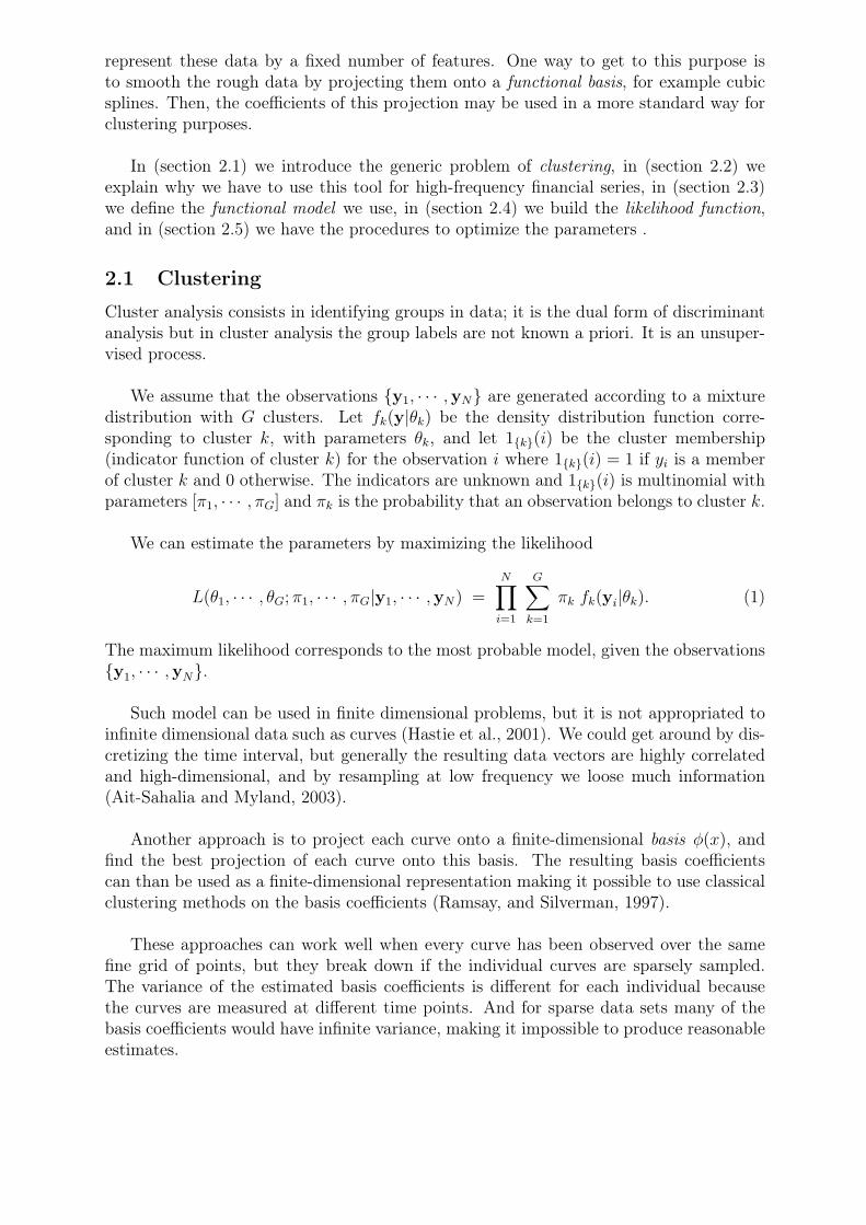
represent these data by a fixed number of features. One way to get to this purpose isto smooth the rough data by projecting them onto a functional basis, for example cubicsplines. Then, the coefficients of this projection may be used in a more standard way forclustering purposes.

In (section 2.1) we introduce the generic problem of clustering, in (section 2.2) weexplain why we have to use this tool for high-frequency financial series, in (section 2.3)we define the functional model we use, in (section 2.4) we build the likelihood function,and in (section 2.5) we have the procedures to optimize the parameters .

2.1 Clustering

Cluster analysis consists in identifying groups in data; it is the dual form of discriminantanalysis but in cluster analysis the group labels are not known a priori. It is an unsuper-vised process.

We assume that the observations {y1, · · · ,yN} are generated according to a mixturedistribution with G clusters. Let fk(y|θk) be the density distribution function corre-sponding to cluster k, with parameters θk, and let 1{k}(i) be the cluster membership(indicator function of cluster k) for the observation i where 1{k}(i) = 1 if yi is a memberof cluster k and 0 otherwise. The indicators are unknown and 1{k}(i) is multinomial withparameters [π1, · · · , πG] and πk is the probability that an observation belongs to cluster k.

We can estimate the parameters by maximizing the likelihood

L(θ1, · · · , θG; π1, · · · , πG|y1, · · · ,yN) =N∏

i=1

G∑

k=1

πk fk(yi|θk). (1)

The maximum likelihood corresponds to the most probable model, given the observations{y1, · · · ,yN}.

Such model can be used in finite dimensional problems, but it is not appropriated toinfinite dimensional data such as curves (Hastie et al., 2001). We could get around by dis-cretizing the time interval, but generally the resulting data vectors are highly correlatedand high-dimensional, and by resampling at low frequency we loose much information(Ait-Sahalia and Myland, 2003).

Another approach is to project each curve onto a finite-dimensional basis φ(x), andfind the best projection of each curve onto this basis. The resulting basis coefficientscan than be used as a finite-dimensional representation making it possible to use classicalclustering methods on the basis coefficients (Ramsay, and Silverman, 1997).

These approaches can work well when every curve has been observed over the samefine grid of points, but they break down if the individual curves are sparsely sampled.The variance of the estimated basis coefficients is different for each individual becausethe curves are measured at different time points. And for sparse data sets many of thebasis coefficients would have infinite variance, making it impossible to produce reasonableestimates.

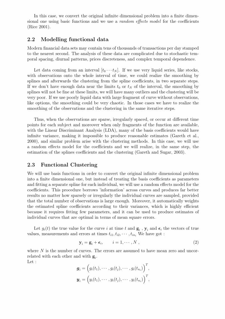
In this case, we convert the original infinite dimensional problem into a finite dimen-sional one using basic functions and we use a random effects model for the coefficients(Rice 2001).

2.2 Modelling functional data

Modern financial data sets may contain tens of thousands of transactions per day stampedto the nearest second. The analysis of these data are complicated due to stochastic tem-poral spacing, diurnal patterns, prices discreteness, and complex temporal dependence.

Let data coming from an interval [t0 · · · tN ]. If we use very liquid series, like stocks,with observations onto the whole interval of time, we could realize the smoothing bysplines and afterwards the clustering from the spline coefficients, in two separate steps.If we don’t have enough data near the limits t0 or tN of the interval, the smoothing bysplines will not be fine at these limits, we will have many outliers and the clustering will bevery poor. If we use poorly liquid data with large fragment of curve without observations,like options, the smoothing could be very chaotic. In those cases we have to realize thesmoothing of the observations and the clustering in the same iterative steps.

Thus, when the observations are sparse, irregularly spaced, or occur at different timepoints for each subject and moreover when only fragments of the function are available,with the Linear Discriminant Analysis (LDA), many of the basis coefficients would haveinfinite variance, making it impossible to produce reasonable estimates (Gareth et al.,2000), and similar problem arise with the clustering methods. In this case, we will usea random effects model for the coefficients and we will realize, in the same step, theestimation of the splines coefficients and the clustering (Gareth and Sugar, 2003).

2.3 Functional Clustering

We will use basis functions in order to convert the original infinite dimensional probleminto a finite dimensional one, but instead of treating the basis coefficients as parametersand fitting a separate spline for each individual, we will use a random effects model for thecoefficients. This procedure borrows ’information’ across curves and produces far betterresults no matter how sparsely or irregularly the individual curves are sampled, providedthat the total number of observations is large enough. Moreover, it automatically weightsthe estimated spline coefficients according to their variances, which is highly efficientbecause it requires fitting few parameters, and it can be used to produce estimates ofindividual curves that are optimal in terms of mean square errors.

Let gi(t) the true value for the curve i at time t and gi , yi and εi the vectors of truevalues, measurements and errors at times ti1, ti2, · · · , tini

We have got :

yi = gi + εi, i = 1, · · · , N , (2)

where N is the number of curves. The errors are assumed to have mean zero and uncor-related with each other and with gi.Let :

gi =(gi(t1), · · · , gi(tj), · · · , gi(tni

))T

,

yi =(yi(t1), · · · , yi(tj), · · · , yi(tni

))T

,

εi =(εi(t1), · · · , εi(tj), · · · , εi(tni

))T

,

where tj is the time-point for the observation j and ni is the number of observations forthe curve i.For the true values gi , we use a functional basis for their representation, and we have :

gi(t) = sT (t) ηi , (3)

where s(t) is the spline basis vector with q dimensions, and ηi is a vector of spline coeffi-cients, (ηi is a Gaussian random variable). Let :

s(t) =(s1(t), · · · , sq(t)

)T

,

ηi =(ηi1, · · · , ηiq

)T

,

If we used a "power cubic spline" with 1 knot, then q = 5 and we would have :

s(t) =(s1(t), · · · , s5(t)

)T

,

with : s1(t) = 1, s2(t) = t, s3(t) = t2, s4(t) = t3, s5(t) = (t− τ)3+, where τ is the knot.

For the Gaussian coefficients ηi we have :

ηi = µzi+ γi , γ ∼ N(0,Γ) , (4)

where zi denotes the unknown cluster membership for the curve i, and it will be treatedas missing data,

zki =

{1 if curve i belongs to cluster k,

0 otherwise,

then we have :P

(zki = 1

)= πk|i ,

µzi=

(µi1zi

, · · · , µiqzi

)T

,

µzi=

{(µ(1))

zi1 · · · (µ(k))zik · · · (µ(G))

ziG}

,

γi =(γi1, · · · , γiq

)T

.

We have split ηi into two terms, µzirepresents the centroid of the cluster and γi represents

the curve in its cluster. Also in the same way, we can represent the centroid of the clusterfrom the global mean of the population by :

µk = λ0 + Λαk , (5)

where λ0 is a (q, 1) vector, and αk (h, 1), Λ is (q, h) matrix, with h ≤ min(q,G− 1).

λ0 =(λ01, · · · , λ0q

)T

,

αk =(αk1, · · · , αkh

)T

,

Λ =

Γ11 · · · Γ1h... . . . ...

Γp1 · · · Γqh

,

With this formulation, the functional clustering model can be written as :

yi = Si(λ0 + Λαzi+ γi) + εi , i = 1, · · · , N , (6)

εi ∼ N(0,R) , γi,∼ N(0,Γ) ,

where Si =[s(ti1), · · · , s(tini

)]T

is the splines basis matrix for the individual i.

Si =

s1(t1) · · · sq(t1)... . . . ...

s1(tni) · · · sq(tni

)

,

αzi=

{(α(1))

zi1 · · · (α(k))zik · · · (α(G))

ziG}

,

but λ0, αk, and Λ could be confounded if no constraints were imposed : Hastie et al.(2001), Therefore we require that :

∑

k

αk = 0 , (7)

that means that s(t)T λ0 may be interpreted as the overall mean curve, and

ΛTSTΣ−1SΛ = I , (8)

with :Σ = σ2I + SΓST ,

where S is the splines basis matrix on a fine grid of time points over the full range of thedata, and we will put R = σ2I, and with Γ the same for every cluster.

Then we have :

• s(t)T λ0 the representation of the global mean curve,

• s(t)T (λ0 + Λαk) the global representation of the centroid of cluster k,

• s(t)TΛαk the local representation of the centroid of cluster k in connection with theglobal mean curve,

• s(t)T γi the local representation of the curve i in connection with the centroid of itscluster k.

2.3.1 Example : Equations for curve i

Let the curve i with ni observations at times {ti1, ti2, · · · , tini}, with gi(t) the unknown

true value, yi(t) the measurement, and εi(t) the measurement error, at time t, and G thenumber of clusters. We have :

yi(t1)...

yi(tni)

=

gi(t1)...

gi(tni)

+

εi(t1)...

εi(tni)

. (9)

We represent the value gi(t) at time t on a spline basis vector s(t), with q dimensions,and ηi the random spline coefficients vector. Then we have :

gi(t) =(s1(t) · · · sq(t)

)

ηi1...

ηiq

, (10)

and an exhaustive description :

gi(t1)...

gi(tni)

=

s1(t1) · · · sq(t1)... . . . ...

s1(tni) · · · sq(tni

)

ηi1...

ηiq

. (11)

We split the random spline coefficients vector ηi into a deterministic coefficients vectorµzi

if the curve i is part of the cluster k defined by the cluster membership zik = 1 andzil = 0 for l 6= k, l = 1 · · ·G, and a random coefficients vector γi :

ηi1...

ηiq

=

µ1...

µq

zi

+

γi1...

γiq

. (12)

We also split the deterministic spline coefficients vector µi into a deterministic coefficientsvector λ0 which represents the coefficients of the global mean curve of all curves, and Λαk

which represents the centroid coefficients of the cluster k from the coefficients of the globalmean curve of the population :

µk1...

µkq

=

λ01...

λ0q

+

λ11 · · · λ1h... . . . ...

λq1 · · · λqh

αk1...

αkh

, (13)

With all these representations, we have got :

yi(t1)...

yi(tni)

=

s1(t1) · · · sq(t1)... . . . ...

s1(tni) · · · sq(tni

)

λ01...

λ0q

+

λ11 · · · λ1h... . . . ...

λq1 · · · λqh

αk1...

αkh

+

γi1...

γiq

+

εi(t1)...

εi(tni)

(14)

2.4 Parametric Identification

Now, we have to estimate the parameters λ0 , Λ , αk , Γ , σ2 et πk by maximization ofa likelihood function.For yi we have a conditional distribution :

yi ∼ N(Si(λ0 + Λαzi

),Σi

),

whereΣi = σ2I + SiΓST

i .

Since the observations of the different curves are independent, the joint distribution of y,and z is given by :

f(y, z) =G∑

k=1

πk1

(2π)n2 |Σ| 12

exp[− 1

2

(y− S(λ0 + Λαz)

)TΣ−1

(y− S(λ0 + Λαz)

)],

(15)

and the likelihood for the parameters πk,λ0,Λ, αk,Γ, σ2, given the observations yi, zi is :

L(πk,λ0,Λ,αk,Γ, σ2|yi, zi) =N∏

i=1

G∑

k=1

πk1

(2π)ni2 |Σi| 12

exp[− 1

2

(yi − Si(λ0 + Λαzi

))T

Σ−1i

(yi − Si(λ0 + Λαzi

))]

.

(16)

Maximizing this likelihood would give us the parameters λ0 , Λ , αk , πk , Γ and σ2 butunfortunately, a direct maximization of this likelihood is a difficult non-convex optimiza-tion problem. If the γi had been observed, then the joint likelihood of yi, zi and γi wouldsimplify, and like zi and γi are independent, the joint distribution can be written as :

f(y, z, γ) = f(y|z,γ)f(z)f(γ) ,

where zi are multinomial (πk), γi are N(0,Γ), and yi are conditional N(Si(λ0+Λαk+

γi); σ2I

).

The joint distribution is now written as :

f(y, z, γ) =1

(2π)n+q

2 |Γ| 12exp

(− 1

2γTΓ−1γ

) G∏

k=1

{πk exp{−1

2n log(σ2)}

exp[− 1

2σ2

(y− S(λ0 + Λαk + γ)

)T (y− S(λ0 + Λαk + γ)

)]}zk

, (17)

and the likelihood of the parameters is given by :

L(πk,λ0,Λ,αk,Γ, σ2|yi, zi,γi) =N∏

i=1

1

(2π)ni+q

2 |Γ| 12exp

(− 1

2γT

i Γ−1γi

) G∏

k=1

{πk exp{−1

2ni log(σ2)}

exp[− 1

2σ2

(yi − Si(λ0 + Λαk + γi)

)T (yi − Si(λ0 + Λαk + γi)

)]}zik

.

(18)

In the paper, we will use the log likelihood :

l(πk,λ0,Λ,αk,Γ, σ2|yi, zi,γi) =

−1

2

N∑i=1

(ni + q) log(2π)

+N∑

i=1

G∑

k=1

zik log(πk) (19)

−1

2

N∑i=1

[log(|Γ|) + γT

i Γ−1γi

](20)

−1

2

N∑i=1

G∑

k=1

zik

[ni log(σ2) +

1

σ2

∥∥yi − Si(λ0 + Λαk + γi)∥∥2

]. (21)

2.5 EM algorithm

The EM algorithm consists of iteratively maximizing the expected values of (19), (20) and(21) given yi and the current parameters estimates. As these three parts involve separateparameters, we can optimize them separately :

2.5.1 E step

The E step is realized from :

γ̂i = E{

γi|yi, λ0,Λ,α,Γ, σ2, zik

}.

For the curve i we have the model :

yi = Si(λ0 + Λαk + γi) + εi .

Let :ui = yi − Si(λ0 + Λαk) ,

then, the joint distribution of ui and of γi is written as :(ui

γi

)∼ N

([00

],

[SΓST + σ2I SΓ

ΓST Γ

]),

and the conditional distribution of γi given ui is :

γi|ui = N(γ̃i;Σγi

),

where :γ̃i =

(ST

i Si + σ2Γ−1)−1

STi ui ,

and :Σγi

= σ2(ST

i Si + σ2Γ−1)−1

.

Then, we have got the conditional distribution for (γ̂i|yi, zik = 1) :

(γ̂i|yi, zik = 1) ∼ N(γ̃i;Σγ̂i

), (22)

with :

γ̃i =(ST

i Si + σ2Γ−1)−1

STi

(yi − Siλ0 − SiΛαk

), (23)

Σγ̂i= σ2

(ST

i Si + σ2Γ−1)−1

. (24)

2.5.2 M step

The M step involve maximizing :

Q = E{

l(πk, λ0,Λ, αk,Γ, σ2|yi, zi, γi)}

,

holding γi fixed

2.5.3 Estimation of π̂k

The expected value of (19) is maximized by setting :

π̂k =1

N

N∑i=1

πk|i , (25)

with :

πk|i = P(zik = 1|yi

),

=f(y|zik = 1)πk∑Gj=1 f(y|zij = 1)πj

,

with : f(y|zik = 1) given by :

yi ∼ N(Si(λ0 + Λαzi),Σi) ,

whereΣi = σ2I + SiΓST

i .

2.5.4 Estimation of Γ̂

The expected value of (20) is maximized by setting :

Γ̂ =1

N

N∑i=1

E[γ̂iγ̂

Ti |Yi

],

=1

N

N∑i=1

G∑

k=1

E[γ̂iγ̂

Ti |yi, zik = 1

], (26)

with (γ̂i|yi, zik = 1) given by the E step.

2.5.5 Estimation of λ0, αk, Λ

To maximize (21), we need an iterative procedure where λ0, αk, and the columns of Λare repeatedly optimized while holding all other parameters fixed.

2.5.6 Estimation of λ0

From the functional model :

yi = Si(λ0 + Λαzi+ γi) + εi , i = 1, · · · , N ,

we have got, by Generalized Least Squares (GLS) :

λ̂0 =( N∑

i=1

STi Si

)−1 N∑i=1

STi

[yi −

G∑

k=1

πk|iSi(Λαk + γ̂ik)]

, (27)

with γ̂ik = E{

γik|zik = 1,yi

}given by the E step.

2.5.7 Estimation of αk

The α̂k are estimated from :

α̂k =( N∑

i=1

πk|iΛTST

i SiΛ)−1

N∑i=1

πk|iΛTST

i

[yi − Siλ̂0 − Siγ̂ik

]. (28)

2.5.8 Estimation of Λ

By GLS, we only have the possibility of estimating vectors and no matrix, thus we willhave to optimize each column of Λ separately, holding all other fixed using :

Λm =( N∑

i=1

G∑

k=1

πk|iα̂2kmST

i Si

)−1

N∑i=1

G∑

k=1

πk|iα̂kmSTi

(yi −

G∑

l 6=m

α̂kmSiΛ̂l − Siγ̂ik

), (29)

where :

• Λm is the column m of Λ

• α̂km is the component m of α̂k

• yi = yi − Siλ̂0

We iterate through (27) (28) (29) until all parameters have converged , then we canoptimize σ2 .

2.5.9 Estimation of σ2

We have got :

σ̂2 =1

N

N∑i=1

G∑

k=1

πkE[(

yi − SiΛαk − Siγi

)T (yi − SiΛαk − Siγi

)|yi, zik = 1]

. (30)

Let :

σ̂2 =1

N

N∑i=1

G∑

k=1

πk

{(yi − SiΛαk − Siγi

)T (yi − SiΛαk − Siγi

)

+Si Cov[γi|yi, zik = 1]STi

}. (31)

The algorithm iterates until all the parameters have converged.

3 Radial Basis Function NetworksRadial Basis Function Networks (RBFN) are neural networks used in approximation andclassification tasks. They share with Multi-Layer Perceptrons the universal approximationproperty (Haykin, 1999). Classical RBF networks have their inputs fully connected tonon-linear units in a single hidden layer. The output of a RBFN is a linear combinationof the hidden units outputs. More precisely, the output is a weighted sum of Gaussianfunctions or kernels (i.e. the nonlinearities) applied to the inputs :

y =I∑

i=1

λi exp{− || x− ci ||2

σi

}, (32)

where x is the input vector, y is the scalar output of the RBFN, ci, 1 ≤ i ≤ I, are thecenters of the I Gaussian kernels, σi, 1 ≤ i ≤ I, are their widths, and λi, 1 ≤ i ≤ I,their weights. Intuitively those last λi parameters represent the relative importance ofeach kernel in the output y. As shown in equation (32), the RBF network has three sets ofparameters ci, σi, λi, 1 ≤ i ≤ I. One advantage of RBFN networks compared to otherapproximation models is that these three sets can be learned separately with suitableperformances. Moreover the learning of the λi weights results from a linear system. Adescription of learning algorithms for RBF networks can be found in (Benoudjit andVerleysen, 2003).

4 The Forecasting MethodIn this section we present a detailed model-based approach for clustering functional dataand a time series forecasting method. This method will first be sketched to give anintuition of how the forecasting is performed. Then each step of the method will bedetailed.

4.1 Method Description

The forecasting method is based on the "looking in the past" principle.

Let’s the observations on the time interval [t0, T ]. To perform a functional predictionof the curve for the time interval [t, t +4tout], we create two functional spaces.A first functional space IN is built with past observations for the time interval [t−4tin, t],the "regressors" and a similar second functional space OUT is built with observations forthe time interval [t−4tin, t+4tout]. These two spaces are built with all data correspond-ing to times t ∈ [t0 +4tin, T −4tin −4tout].

These functional spaces are combined into a probabilistic way to build the functionalprediction for the time interval [t, t+4tout] and are quantized using the functional cluster-ing algorithm. The relationship between the first and the second functional spaces issuedfrom the clustering algorithms is encoded into a probability transition table constructedempirically on the datasets.

In each of the clusters determined by the second clustering OUT , a local RBFN modelis built to approximate the relationship between the functional output (the local predic-

tion) and the functional input (the regressor).

Finally, the global functional prediction at time t for the interval [t, t + 4tout] isperformed by combining the local models results associated to clusters OUT , accordingto their frequencies with respect to the class considered in the cluster IN .

4.2 Quantizing the « inputs »

Consider a scalar time series X, where x(t) is the value at time t, t ∈ [t0, T ]. This originalseries is transformed into an array of observations Xin for the time intervals [t, t +4tin],for all t ∈ [t0, t0 +4tin, t0 + 24tin, · · · , T −4tin −4tout].Then the clustering algorithm is applied to the input array Xin; after convergence it givesan IN map of Kin codewords and the spline coefficients for the curves of each cluster inthis IN map .

4.3 Quantizing the « outputs »

At each input vector of the matrix Xin we aggregate the next observations to get anew array Yout for the time interval [t, t + 4tin + 4tout] for all t ∈ [t0, t0 + 4tin, t0 +24tin, · · · , T −4tin −4tout].The clustering algorithm is applied to the new array Yout; after convergence it gives anOUT map of Kout codewords and the spline coefficients for the curves of each cluster inthis OUT map.Note that, by construction, there is a one-to-one relationship between each input and eachoutput vector of spline coefficients.

4.4 Probability transition table

Both sets of codewords from maps IN and OUT only contain a static information. Thisinformation does not reflect completely the evolution of the time series.The idea is thus to create a data structure that represents the dynamics of the time series,i.e. how each class of output vectors of spline coefficients (including the values for thetime interval [t, t+4tout]) is associated to each class of input vectors of spline coefficientsfor the time interval [t−4tin, t].This structure is the probability transition table T (i, j), with 1 ≤ i ≤ Nin, 1 ≤ j ≤ Nout.

Each element T (i, j) of this table represents the proportion of output vectors thatbelongs to the jth class of the OUT map while their corresponding input vectors belong toclass i of the IN map. Those proportions are computed empirically for the given datasetand sum to one on each line of the table.Intuitively the probability transition table represents all the possible evolutions at a giventime t together with the probability that they effectively happen.

4.5 Local RBFN models

When applied to the « outputs », the functional clustering algorithm provides Nout classesand the spline coefficients of the curves for the intervals [t, t + 4tout]. In each of theseclasses a RBFN model is learned.Each RBFN model has p inputs (the spline’s coefficients of the regressors) and q outputs

(the spline coefficients of the prediction curve).

These models represent the local evolution of the time series, restricted to a specificclass of regressors. The local information provided by these models will be used whenpredicting the future evolution of the time series.

4.6 Forecasting

The relevant information has been extracted from the time series through both maps, theprobability transition table and the local RBFN models detailed in the previous sections.Having this information, it is now possible to perform the forecasting itself.

At each time t, the goal is to estimate the functional curve for the time interval[t, t +4tout] denoted x̂([t, t +4tout]).

First the input at time t is built, leading to X(t). This vector is presented to the INmap, and the nearest codeword Xk(t) is identified (1 ≤ k(t) ≤ Nin).

In the frequency table, in the k(t)th line, there are some columns corresponding toclasses of the OUT map for which the proportions are non zero. This means that thosecolumns represent possible evolutions for the considered data X(t), since X(t) has thesame shape than data in the k(t)th class.

For each of those potential evolutions, the respective RBFN models are considered(one RBFN model has been built for each class in the OUT map).For each of them, a local prediction x̂j([t, t +4tout]) is obtained (1 ≤ j ≤ Nout).

The final prediction is a weighted sum of the different local predictions, the weightsbeing the proportions recorded in the probability transition table.

The final prediction is thus :

x̂([t, t +4tout]) =Nout∑j=1

T (k, j)x̂j([t, t +4tout]). (33)

5 Experimental ResultsThe examples presented here deal with the IBM stock time series of "tick data" for theperiod starting on January 02, 1997 and ending on may 08, 1997 with more than 3000transactions per day, on the New York Stock Exchange (NYSE).

The pricing model will use as inputs, inhomogeneous and high-frequency time se-ries of bid and ask prices and also implied volatility. Such volatility time series can beobtained from market data, derived from option market prices(from eight call and putnear-the-money, nearby and secondary nearby option contracts on the underlying asset)orcomputed from diverse model assumptions.

On Fig. 1 we can see the evolution of the Prices (top) and Volumes (bottom) on oneday.

On Fig. 2 we see the distribution of transactions for the same day. Each point is atransaction, with more transactions at the opening and closing of the NYSE.The transactions are sampled discretely in time and like it is often the case with financialdata the time separating successive observations is itself random.On Fig. 3 we can see two successive days of the stock IBM with a fine smoothing of the"tick data" by splines.

10:00 11:00 12:00 13:00 14:00 15:00 16:00163.5

164

164.5

165

165.5

166

Time of the Day

Pric

es U

S $

TRANSACTIONS on Day 12

10:00 11:00 12:00 13:00 14:00 15:00 16:00

0

5

10

15

x 104

Time of the Day

Vol

umes

Figure 1: Prices (Top) et Volumes (Bottom)

09.30__

TRANSACTIONS between 09.30 hr and 16.00 hr on Day 12

10.00__

10.30__

11.00__

11.30__

12.00__

12.30__

13.00__

13.30__

14.00__

14.30__

15.00__

15.30 16:00

15.30__

Time of the Day

Figure 2: Distributions of transactions

0.2 0.4 0.6 0.8 1 1.2 1.4 1.6 1.8 2 2.2

x 104

163

164

165

166

167

168

169

170

Time of the day in Secondes

Pric

es U

S $

Transactions on Day 10

0.2 0.4 0.6 0.8 1 1.2 1.4 1.6 1.8 2 2.2

x 104

163

163.5

164

164.5

165

165.5

166

166.5

167

167.5

168

Time of the day in Secondes

Pric

es U

S $

Transactions on Day 11

Figure 3: Two days of transactions for IBM (dashed curve),with smoothing splines (solid curve)

5.1 Prediction

We forecast the future transactions splines for three hours of day J between 10.30Hr. and13.30 Hr. (4tout = 3.0Hr), from the past transactions (days J − 2 and J − 1 and half anhour of day J between 10.00 Hr. and 10.30 Hr.), in this case (4tin = 11.30Hr).We have eliminated the transactions at the opening and closing of the NYSE, which are"outliers" without any correlation with the next hours.

On Fig. 4 we can see four out-of-sample forecasting days superposed with the obser-vations and smoothing splines (not known by the model). There is a good correlation

between the out-of-sample forecasting and the observations.

11:00 11:30 12:00 12:30 13:00

151.5

152

152.5

153

153.5

154

Pric

es

Observations, Spline and Prediction

11:00 11:30 12:00 12:30 13:00

152.5

153

153.5

154

154.5

155

Pric

es

Observations, Spline and Prediction

11:00 11:30 12:00 12:30 13:00

148

148.5

149

149.5

150

150.5

Pric

es

Observations, Spline and Prediction

11:00 11:30 12:00 12:30 13:00

152

152.5

153

153.5

154

154.5

Pric

es

Observations, Spline and Prediction

Figure 4: Four forecasting days for IBM stock price. Observations (Points); Smoothing splines(solid curve); Out-of-sample forecasting by the model (dashed curve)

6 ConclusionWe have presented a functional method for the clustering, modelling and forecasting oftime series by functional analysis and neural networks. This method can be applied toany types of time series but is particularly effective when the observations are sparse,irregularly spaced, occur at different time points for each curve, or when only fragmentsof the curves are observed; standard methods completely fail in these circumstances.By the functional clustering, we can also realize the forecasting of multiple dynamicprocesses.

ReferencesAit-Sahalia, Y. and P.A. Myland,(March, 2003),”The effects of random and discrete sam-

pling when estimating continuous-time diffusions”,Econometrica, Vol. 71, pp. 483-549.

Benoudjit, N. and M. Verleysen, ”On the kernel widths in Radial-Basis Function Net-works”, Neural Processing Letters, Kluwer academic pub., vol. 18, no. 2, pp. 139-154,October 2003.

Box, G. and G.M. Jenkins,(1970), ” Time series Forecasting and Control ”, Holden-Day ,

de Boor, C. (1978), ” A Practical Guide to Splines ”, New York : Springer ,

Dempster,A.P., N.M. Laird, and D.B. Rubin,(1977), ”Maximum likelihood from incom-plete data via the EM algorithm ”, Jounal of the Royal Statistical Society, Ser. B , Vol.39, pp. 1-22.

Diebold, F., J.H. Lee and G.Weinbach, ”Regime switching with time-varying transitionprobabilities, in non stationary time series analysis and cointegration”, ed. by C. Har-greaves, 1994, pp 283-302, Oxford University Press.

Engel, R.F., ”Autoregressive Conditional Heteroscedasticity with Estimates of the Vari-ance of United Kingdom Inflation”,Econometrica, Vol. 50, pp. 987-1007, 1982.

Fama, E.F., ”Efficient Capital Markets : II”,The Journal of Finance, Vol. XLVI, N◦ 5, pp.1515-1617, 1991.

Hamilton, J.D.,(1994), ” Time Series Analysis ”, Princeton University Press ,

Hastie, T., R. Tibshirani, and J. Friedman ,(2001), ’ ” The Elements of Statistical Learn-ing. dta Mining, Inference, and prediction ”, Springer ,

Haykin, S.,(1999), ” Neural Networks - A comprehensive foundation ”, Prentice Hall,

Franke, G., R. Olsen and W. Pohlmeier,(June 2002), ”Overview of Forecasting Mod-els”,University of Konstanz, Seminar on High Frequency Finance, paper SS 2002.

James, G.M., T.H. Hastie and C.A. Sugar,(2000), ”Principal component models for sparsefunctional data”, Biometrika, Vol. 87, pp. 587-602.

James, G.M., C.A. Sugar,(2003), ”Clustering for sparcely sampled functional data”, Jour-nal of the Americal Association, Vol. 98, pp. 397-408.

Ramsay, J.O., and B.W. Silverman,(1997), ” Functional Data Analysis ”, Springer Seriesin Statistics,

Rice, J.A. and C.O. Wu,(March 2001), ”Nonpoarametric Mixed Effects models for Un-equally Sampled Noisy Curves”,Biometrics, Vol. 57, pp. 253-259.

Olsen, R.B. and M.M. Dacorogna,(December 1992), ”going Back to the Basics - RethinkingMarket Efficiency”,Olsen and Associates research Group, Paper RBO.1992-09-07.