
Modelling and Forecasting Demand for Nepali Tourism · Modelling and Forecasting Demand for Nepali...
32
Modelling and Forecasting Demand for Nepali Tourism Shoora B. Paudyal, Ph.D. * Abstract In this paper international demand for Nepali tourism from the selected major markets has been estimated using time series data of number of tourist arrivals, per capita income, own price and prices of related goods. Autoregressive distributive lagged (ARDL) models are applied as a tool of estimation. This study confirms that tourism demand for Nepal is the composite function of disposable income, own price, cross price, lags of these variables, word of mouth of the visitors and qualitative factors captured by dummies. The most important policy implication can be derived from the words of mouth of the visitors. This manifests that only the good impression on the visitors can generates better words of mounth in favour of destination which underscores the up-gradation of the tourist products for the better image of the destination. The best performed models are used for forecasting the growth rates of tourist arrivals from the eight major markets for 2010 to 2020. The forecasted growth rates of tourist arrivals from major eight market are found very close to the actual average annual growth rates for 2006 to 2010. Key Words: Demand, Modelling, ARDL Model, Diagnostic Tests, Restrictive Models, Wickens-Bruesch ECM, Johansen Maximum Likelihood ECM, Forecasts. JEL Classification: C13, C22, L83, O47 * Dr Paudyal is associated with Central Department of Economics, Tribhuvan University, Kathmandu. Email: [email protected] The author acknowledges the valuable comments and suggestions given by Dr. Min B. Shrestha and other members of editorial board as well as by the external reviewers. However, the author is solely responsible for the errors.
Transcript of Modelling and Forecasting Demand for Nepali Tourism · Modelling and Forecasting Demand for Nepali...

Modelling and Forecasting Demand for Nepali Tourism
Shoora B. Paudyal, Ph.D.*
Abstract In this paper international demand for Nepali tourism from the selected major markets has been estimated using time series data of number of tourist arrivals, per capita income, own price and prices of related goods. Autoregressive distributive lagged (ARDL) models are applied as a tool of estimation. This study confirms that tourism demand for Nepal is the composite function of disposable income, own price, cross price, lags of these variables, word of mouth of the visitors and qualitative factors captured by dummies. The most important policy implication can be derived from the words of mouth of the visitors. This manifests that only the good impression on the visitors can generates better words of mounth in favour of destination which underscores the up-gradation of the tourist products for the better image of the destination. The best performed models are used for forecasting the growth rates of tourist arrivals from the eight major markets for 2010 to 2020. The forecasted growth rates of tourist arrivals from major eight market are found very close to the actual average annual growth rates for 2006 to 2010.
Key Words: Demand, Modelling, ARDL Model, Diagnostic Tests, Restrictive Models, Wickens-Bruesch ECM, Johansen Maximum Likelihood ECM, Forecasts. JEL Classification: C13, C22, L83, O47
* Dr Paudyal is associated with Central Department of Economics, Tribhuvan University,
Kathmandu. Email: [email protected]
The author acknowledges the valuable comments and suggestions given by Dr. Min B. Shrestha and other members of editorial board as well as by the external reviewers. However, the author is solely responsible for the errors.
Modelling and Forecasting Demand for Nepali Tourism
59
I. INTRODUCTION Tourism can play a greater role in economic growth of an developing landlocked country like Nepal. With its higher potentialities in tourism development, Nepal is often considered that it can make a headway in development with a greater emphasis on the development of tourism. However, its contribution so far has been inadequate as compared to its development potentialities. In this context, this paper aims to examine the demand aspect of Nepali tourism in the international markets and try to provide feed back to the government policy interventions.
II. THE CONCEPTUAL FRAMEWORK According to the standard Marshallian analysis, demand for a commodity is a function of its own price, prices of close substitutes, disposable income, tastes and so on. In the Marshallian theory of consumer demand, a tourist is a consumer who derives utilities from the consumption of a basket of goods. Travelling is one of the items in his/her basket. With a given budget and prices, a consumer has to distribute his/her income across various purchases of goods so as to maximize total utility. Symbolically,
Max U (T, Qo) Subject to the budget constraint PoQo + PtT = I ………. (1) where U = utility function, T= quantity of tourism products, Qo = other goods in the basket, Po = price of other goods, Pt = price of tourism products and I = income or consumer's budget. By solving the Lagrangian Multiplier, we can derive the tourism demand function for a consumer as follows: L = U (T, Qo) - λ(PoQo + PtT-I ………. (2) From this we can derive the following tourism demand function: T = F(PtT, PoQo, I) ………. (3) In the simplest case, demand for any particular good including travelling depends on disposable income of the consumer and relative prices. It is noteworthy here that a visit or trip is one of the many commodities in the consumer's market basket. The demands for non-tourism consumer goods such as food, clothing and shelter are more fundamental and are the basic means for survival and to live a decent life for people. A household or individual is more likely to forego a vacation than to be deprived of these essential things. Hence, during

NRB ECONOMIC REVIEW
60
a time of economic instability and economic recession, households are more likely to reduce the consumption of an expensive commodity such as tourism. Thus travelling does not come under the category of basic necessary goods. The high income elasticity of tourism demand suggests that travel depends strongly on the consumption climate and economic expectation (Smeral,1988: 38) which implies income elasticity of travel demand is greater than one.
Allocation model (Smeral, 1988: 39) states that private consumption depends on the demand for non-tourism consumer goods in generating countries, domestic consumption of tourism services by the country, tourism consumption abroad, prices of non-tourism consumer goods in tourist generating country (expressed as units of homogeneous currency), prices of foreign tourism goods and services in units of a homogeneous currency, disposable income in units of a homogeneous international currency. He shows in that model that demand for every consumer good, including tourism, is a function of disposable income and prices (own price and related prices). Saving is regarded as future consumption.
According to the travel cost demand model, the cost of a tourism trip varies with distance between market and destination, and per capita income, which is considered to be a good measure to determine the budget of a tourist going abroad. In addition, relative prices of goods and services in a destination and an alternative destination also affect the visits of people. Linguistic affinity and cultural proximity also attract more visitors along with safety and security in the destination. Based on these theories and data limitations we can rewrite equation (iii) as follows:
V = v(P, Pr, I) ………. (4)
where, V is tourism demand or visitors’ demand in the host country. As it is not possible here to seggregate the price of tourism products and that of other products. So consumer’s price index ratio between destination country and the country of tourist origin measure relative consumer’s price, Pt+Po = P in the destination country. So P stands as a relative price index in the destination country, Pr as relative price index in the alternative destination and I is the per capita income in visitors’ country. From the theoretical framework, one can hypothesize for the purpose of tourism demand modelling as follows:
dV/dI > 0; dV/dP < 0; dV/dPr>0; if the related destination is substitute dV/dPr<0; if the related destination is complement ………. (5)
A tourist is a temporary visitor to the host country. The word tourist is derived from the word “tour”. A tour is the visit. The WTO (Holloway, 1998:2) defines tourists as “any person visiting a country other than that in which he has his usual residence; for any reason other than following an occupation remunerated from within the country visited." Demand is defined as a schedule or measure of the quantity of any good or service which consumers are willing to purchase and are able to buy at specific price during a specific time period. However, demand can be categorised as actual or effective demand,as well as

Modelling and Forecasting Demand for Nepali Tourism
61
potential demand and deferred demand. The most important factors governing demand are disposable income and the prices of own and related goods and services. The distribution of income, value of currency, tax policy, population, etc. are other variables in the demand function. Demand for travelling, thus, is a composite function of the disposable income, taste, fashion, own price, prices of close substitutes and monetary and opportunity costs of the traveller. Moreover, tourism demand is highly sensitive to socio-political changes and seasonality as well as social factors such as attitudes and behaviour of natives toward foreigners (Kaul, 1994). Friendly behaviour of natives toward the foreign visitors promotes the destination on the international market. Likewise, political stability and peace as well as the safety of visitors are taken as the prerequisites to attract more international visitors to the destination. If all other things remain the same, own price is negatively related with the amount of goods and services demanded by the individual consumer. This specific relationship between price and quantity demanded is called as the “law of demand”. So far as tourism economics is concerned, the actual number of visitors is the active participants in tourism who visit the destinations where they can demand the local goods and services. For this reason, consumers or visitors need to be present physically to consume tourism services in the host countries. The number of visitors is easily measured and thus, it is commonly used as a proxy measure of demand for tourism in the host countries. Demand for travel primarily depends on the willingness to travel and ability to pay for travelling. However, willingness to travel can be explained partly in terms of the distance, since the longer the distance the higher the time and money costs involved (Paudyal, 1993; 1998). However, this is now considered as a less influencing factor in the face of increasingly competitive cheaper airfares. In spite of this, regional tourism with short time holidays is on the rise in the Europe and the Americas. There are other motivational factors that generate the willingness to travel of the people, such as sun, sand and sex (English, 1986), desire to explore diverse culture and places with different tastes and flavours. Above all, a rise in real wage and paid holidays have raised the ability of the individuals to pay for luxurious goods like tourism. Becker theory (1965) reveals how the importance of leisure time has increased with the rise in wage level. Ability to pay for tourism is thus a function of price and income variables. A visit or trip is one of the many “commodities” in the individual consumer's basket. Hence, a tour is itself a consumer's commodity which can be supplied and demanded, i.e., a tour offer from destination is supply and decision to travel to a specific destination is demand. The number of tourists to a country, thus, expresses the demand for tourism in the tourist receiving country. The visit of people to the destination is the demand for that destination. The visitors are the consumers of the tourism services offered in the destination. The price paid for a tour or visit is the airfare to get to the destination country plus the tourist's expenditure on hotel, food and beverages, local touring and travel, transport, souvenirs and some others. The tourism market is a monopolistic one and therefore, individuals are assumed to have an imperfect knowledge about the market. This gives rise to the importance of advertisement in
NRB ECONOMIC REVIEW
62
the tourism business. Informative advertisement and promotional activities are always desirable in the tourism business so as to create temptation and desire, thus affecting the individuals’ travel motivation to go for holidays into a particular destination among many alternatives and thereby make the upward shift in the individual demand curve for travel and tourism in a specific destination. The demand for Nepal’s tourism is a part of the South Asian tourism demand and a small fraction world tourism demand. The demand for tourism in the world tourism market has grown with the rapid growth of economies in the West. Hence, the growth in demand for tourism and the tourism market can be primarily attributed to the great success of the capitalist economy during the 1950s and 1960s. Moreover, a faster spread of air linkages and speedy jet aero planes contributed to an increase in the demand for tourism in far distant destinations such as Nepal.
III. MODELLING TOURISM DEMAND Even though econometric modelling for tourism demand is a complicated work, it has become general practice in many countries. It has been used in many countries for the analysis of past trends and for the prediction of future pattern of tourist arrivals in the country so as to contribute to state’s tourism policies. The research studies on tourism demand with future prediction have helped the government enormously in policy formulation for the development of tourism sector. A review of the tourism demand modelling in the past gives some glimpses that tourism modelling traditionally can be categorised as a ‘simple to general model’, because, modellers have often formulated multi-variable single equation models including demand determinants based on demand theory. However, they frequently have dropped some variables and replaced them by new variables to get better results, especially when the results from the initial regressions found to have suffered from multicolinearity or heteroskedasticity or serial correlation, etc. In such cases they, most often, pay little attention to the theoretical and conceptual framework. As a result tourism demand modelling has switched off from a specific model (to economic theory) to a general demand model (Hendry, 1995; Song et al. 2003). Modellers are now well aware that the economic time series such as GDP, price, and saving contain a unit root; a test for this is imperative before such series are used for a regression (Gujrati 2007 and Pindyck et al 1991). Modelling demand for tourism varies from writer to writer. As Morley (1991:40) writes:
Multiple regression is used widely as a tool for the estimation of tourism demand functions. Problems of heteroskedasticity, multicolinearity, and autocorrelation are well recognized by modellers, but questions of model specifications are less widely understood. Misspecification of the model, such as failure to include an important explanatory variable or a wrong functional form, can have significant impacts on the model estimated.

Modelling and Forecasting Demand for Nepali Tourism
63
However, the most widely used model is one in which the explanatory variables are multiplicative and a logarithmic transformation linear equation. We refer this here as log-log model. Johnson and et al (1990:147) writes:
Virtually all the studies utilize a log linear model form, which has the convenient property that coefficients represents estimates of a constant elasticity value. Some investigators (Kliman, 1981; Uysal and Crompton, 1984) report trying the linear form, but obtaining inferior results to log linear form.
This might be the reason that most of the modellers use a lagged model for demand studies. Most of the OLS regressions are run on a double log model (Bwire, 1987; Woo, 1992; NRB, 1988; Paudyal 1993, 1998, 2013, Pye and Lin, 1983; Krause and Jude, 1973). Some authors have used an input-output analysis (Burger, 1978), others a benefit-cost model (Mitchell, 1971; Mathematica, 1970). Pye and Lin (1983) estimate the demand for tourism in Hong Kong. The demand for tourism is estimated for Hong Kong covering 1962-78. They find both tourist expenditure and arrival demand highly income elastic. Unlike the time-series analysis, they find both tourist arrival and tourist expenditure income inelastic in cross section estimation. They reveal that merchandise trade is an important variable in tourism demand for Hong Kong. Krause et al (1973) estimate tourism demand for 17 Latin American countries. They find that income variable is an important variable for 11 countries but the price variable not significant one. The first study on Nepali tourism uses an input-output model (Burger, 1978). It tries to measure the economic impact of tourism. The other studies (NRB, 1989; Paudyal 1993) carry out an econometric study using cross-section and time series data. NRB (1989) study finds that tourism demand is income inelastic in case of both dependent variables (tourist arrival and tourist expenditure). Tourist expenditure is found to be highly sensitive with respect to exchange rate but the least with tourist arrival. The sign of the exchange rate variable is found as a priori expectation. Paudyal (1993) finds that demand is income elastic in case of tourist arrivals. Ordinary least square is the most popular tool and procedure for the estimation of tourism demand and its elasticity. A double log model is widely used for tourism demand. Recently in this decade, tourism demand modelling witnesses a land mark paradigm shift in its methodology, popularly known as ‘general to specific’ modelling method. The specification of such model starts with including all possible variables permitted by economic theory as independent variables to explain tourism demand and then the lagged forms of all independent variables and that of dependent variable are also incorporated in this model as explanatory variables. This is popularly known as an autoregressive distributive lagged model or ARDL model of general form. The merit of ARDL model is that the estimation of an equation helps further proceed to a more efficient specific model with more degree of freedom.
NRB ECONOMIC REVIEW
64
In the recent years for the time series time ARDL model has been popular. From the estimation of a general ARDL model, one can get the idea to go for estimating several types of restricted models including reduced ARDL model. Restricted specific models are tested to find out whether they are valid. Only in the case a specific model passes its validity test gives a green signal for estimation of tourism demand using that model. Various diagnostic tests are needed to be carried out to examine the performance of the various specific models for best fit, such as the White chi-square test for heteroskedasticity, the Lagrange multiplier (LM) test for serial correlation, the Chow test for predictive failure, the Ramsey reset test for misspecification, and the J-B chi-square test for non-normality.
IV. METHODOLOGY For the econometric modelling for tourism demand, data are collected from publications of international institutions and from government agencies in Nepal. The data on the number of visitors are collected from various issues of Nepal Tourism Statistics, published by Ministry of Tourism and Civil Aviation (MoTCA,G/N). Because of data limitation, Indian demand for Nepali tourism is estimated using data from 1974 to 2009, while data from 1962 to 2009 are utilised for rest of market demand. Tourist data on the consumer price index, population, gross domestic product and exchange rate are obtained from the various issues of the IMF publication, International Financial Statistics Yearbook. The data are processed using Eviews 5. The empirical study on demand for Nepali tourism from eight countries of origin are analysed. These markets are as follows: Australia, France, Germany, India, Japan, Spain, UK and USA. These markets together make over 50% of the total arrivals in 2009. Many of them are included in the list of top 15 outbound tourism markets in the world. Estimating tourism demand for each individual market, general ARDL modelling is used . This is a multi-variable single equation model with lag variables of both dependent and independent variables. Besides, this model incorporates several dummies to capture the instabilities that occurs due to political and social disturbances. The general ARDL model takes the following form (Hendry, 1995; Song et al. 2003):
tit
l
jiijt
k
j
l
i ji dummiesYbXaaY ε++++= −=
−= = ∑∑ ∑1
1 00 ………. (6)
Where Y is a dependent variable, that is tourism demand, and Xs are explanatory or independent variables, l is lag length and k is the number of explanatory or independent variables. a0 is intercept and as and bs are slope coefficient parameters to be estimated from the equation. Based on tourism demand theory, the demand for Nepali tourism from various markets (countries of tourist origin) is modelled by the estimation. Now, dependent variable Y is replaced by visit, i.e. quantity of tourism demanded i.e. number of tourist arrivals and independent variables Xs are replaced by own price, price of related goods, and real percapita income.

Modelling and Forecasting Demand for Nepali Tourism
65
lvt = β0 + β1lvt-1 + µ0lpcit + µ1lpcit-1+ φ0lcpit + φ1lcpit-1 + α0lcpiit + α1lcpiit-1 + dummies + εt ………. (7)
This means that tourism demand (lvt) is a function of the log lagged dependent variable i.e., visitors (lvt-1), the log of per capita real gross domestic income in the tourist generating country (lpcit), the log lagged income variable (lpcit-1), the log of relative consumer price index in host country as compared to country of origin (lcpit) that is a price variable, the log lagged consumer price index (lcpit-1), the log of relative consumer price index of substitute or complementary destination (lcpiit), the log of lagged relative consumer price index of related destination (lcpiit-1), and dummies. The number of tourist arrivals is a proxy variable for the demand for tourism in Nepal. Demand is positively related to disposable income. Likewise, per capita real GDP in country of origin measured in national currency is taken as a proxy variable for disposable income. As disposable income increases, demand for all normal goods including travel and tourism also increases. A foreign trip is assumed to be a normal commodity in a rational consumer’s demand basket. Another variable is the price in the demand function. This variable is defined as the consumer price index in tourist receiving country divided by the consumer price index in the visitor's country. The law of demand says that the higher the relative price of that commodity in the market the lower is the demand for that commodity. Visitors are assumed to compare prices of the commodities in the host country with that of their own country. Hence, it is assumed here that the tourist inflow is inversely related to the relative consumer price index in the tourist receiving countries. The relative price index is adjusted with the real exchange rate between sending and destination countries. The real exchange rate is the ratio of nominal exchange rate divided by the consumer price index in the tourist receiving country multiplied by the consumer price index in the United States. Furthermore, cross price variable is considered in the demand function. The related goods can be either complementary or substitute. India as a destination for overseas visitors may be a substitute or complementary destination for Nepal. So, the consumer price index in India is divided by the consumer price index in the tourism market, which is taken as the prices of related goods and services in the Nepal destination and adjusted with real exchange rate between country of origin and India. Aforementioned Indian tourism can be either a complementary or substitute destination for Nepali tourism. If former is the case, higher prices of commodity in India as compared to Nepal reduces demand for Nepali tourism, i.e., there will be less tourist arrivals in Nepal and India. In other words, there will be an inverse relationship between relative price index in India and demand for Nepali tourism. So this variable will have a negative expected sign. Nepal and India can jointly promote the tourism of both countries in the country of origin. On the other hand, if latter is the case there will be positive relationship between tourism demand in Nepal and relative price in India. So, cross price variable will have negative expected sign. Higher relative prices in India will bring an increase in demand for Nepali
NRB ECONOMIC REVIEW
66
tourism, i.e. there will be a positive relationship between the relative price index in India and demand for Nepali tourism. In this case, India is a competitor to the Nepali tourism, it will be more challenging to the Nepali tourism. Dummy variables are considered to capture the effects of political and other instabilities that impact on the arrivals. Dummy variable considered here are as follows: Oil crisis in 1974 and in 1979: (dum74) and (dum79); Political disturbance and referendum in 1979,1980 (dum80), Middle east crisis in 1981(dum81), Assassination of Indira Gandhi in 1984 (dum84), 31 October; Trade embargo of India in 1989 (dum89), Gulf war in 1990 and 1991(dum90) and (dum91); Demolition of Babari Mosque in 1992 December (dum92); Visit Nepal Year 1998, (Dum98), Indian airline hijack from Kathmandu in 1999 December (Dum00); Asian crisis 1998 and 1999 to capture the effects of Asian financial crisis; Ritik Roshan riot in Kathmandu in 2000 December (Dum00), Royal massacre/September 11, 2001 (Dum01), Strikes for republic in Nepal, 2005 (Dum05), Great recession in 2008 (Dum 08). Among these some of the dummy is India specific, such as a trade embargo in India. Unit root tests are carried out to detect whether various time series are non-stationary. Almost all time series in different markets are found to be non stationary at I (0) and stationary at I (1). However, when these time series are combined for the regression estimates, they are found to be stationary with ARDL and specific models. The regression results for tourism demand, using the auto regressive distributive lagged (ARDL) general model are given in table 1 (Annex). The results show that among estimated coefficients for all independent and lagged visitor variables, the latter is found highly significant even at a 5% level, indicating that word of mouth is a very influential factor in tourism demand. It insists that the demand for the Nepali tourism features a stable behaviourial pattern or is habit persistent. Dummy80 is significant only for Australia, Spain and the USA, i.e., referendum and political disturbance did not disturb arrivals from other countries except Australia and the USA. Dummy84 is found significant for Australia and Japan implies that disturbances created by the assassination of Indira Gandhi are influential variables for those markets. Dummy89 and Dummy00, which stand for trade embargo and Indian plan hijacked from Kathmandu respectively, are the most influential events in the case of the tourist arrivals from India. Dummy01 (September 11/Royal massacre) is significant for all markets considered in this study, and dummy05 (strikes for the republic) is found significant for Australia, France, Japan and the USA. Moreover, the models for majority markets explain more than 90% of the variation in tourist arrivals in the country and DW statistics are close to 2 indicating models are not suffered from positive and native serial correlation. However, a higher adjusted R2 with a few significant t-statistics in almost all models is the indication that these models mgih have suffered from the multicolinearity problems. In the last, the best performed models are used for forecasting the growth rates of tourist arrivals from the eight major markets for 2010 to 2020. Various independent variables are forecasted by using Hodrick-Prescot Filter, a smoothing method. Different measures for forecasting error magnitudes have been available for the evaluations of forecasting tourism demand. The lower the forecasting magnitudes of the models the higher the fitness of data for the country specific models. Among various measures, the predominantly used measures are Theil U, Root Mean Square Error, Mean
Modelling and Forecasting Demand for Nepali Tourism
67
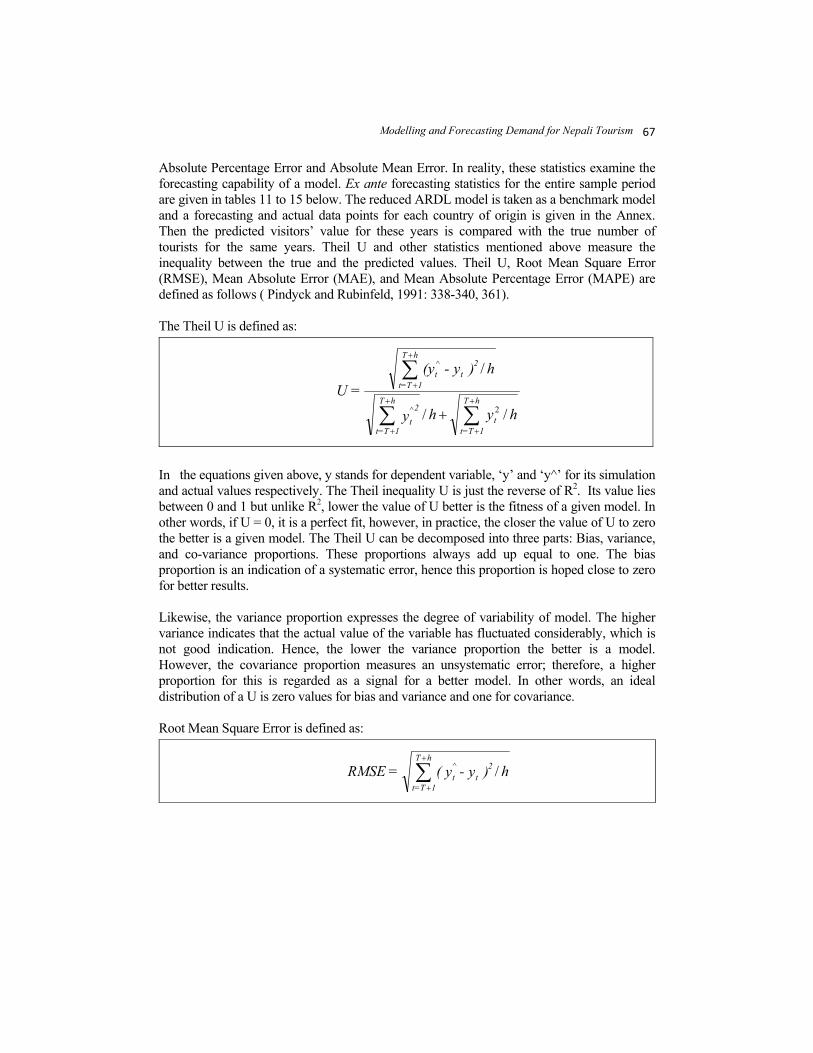
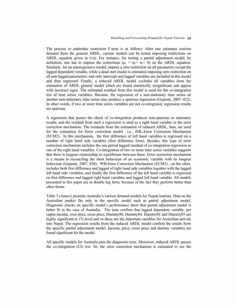
Absolute Percentage Error and Absolute Mean Error. In reality, these statistics examine the forecasting capability of a model. Ex ante forecasting statistics for the entire sample period are given in tables 11 to 15 below. The reduced ARDL model is taken as a benchmark model and a forecasting and actual data points for each country of origin is given in the Annex. Then the predicted visitors’ value for these years is compared with the true number of tourists for the same years. Theil U and other statistics mentioned above measure the inequality between the true and the predicted values. Theil U, Root Mean Square Error (RMSE), Mean Absolute Error (MAE), and Mean Absolute Percentage Error (MAPE) are defined as follows ( Pindyck and Rubinfeld, 1991: 338-340, 361). The Theil U is defined as:
In the equations given above, y stands for dependent variable, ‘y’ and ‘y^’ for its simulation and actual values respectively. The Theil inequality U is just the reverse of R2. Its value lies between 0 and 1 but unlike R2, lower the value of U better is the fitness of a given model. In other words, if U = 0, it is a perfect fit, however, in practice, the closer the value of U to zero the better is a given model. The Theil U can be decomposed into three parts: Bias, variance, and co-variance proportions. These proportions always add up equal to one. The bias proportion is an indication of a systematic error, hence this proportion is hoped close to zero for better results. Likewise, the variance proportion expresses the degree of variability of model. The higher variance indicates that the actual value of the variable has fluctuated considerably, which is not good indication. Hence, the lower the variance proportion the better is a model. However, the covariance proportion measures an unsystematic error; therefore, a higher proportion for this is regarded as a signal for a better model. In other words, an ideal distribution of a U is zero values for bias and variance and one for covariance. Root Mean Square Error is defined as:
hyhy
h)y-(y=U
t
hT
1T=tt
2hT
1T=t
2tt
hT
1T=t
//
/
2^
^
∑∑
∑+
+
+
+
+
+
+
h)y-y(=RMSE 2tt
hT
1T=t
/^∑+
+

NRB ECONOMIC REVIEW
68
Mean Absolute Error is defined as:
Mean Absolute Percentage Error is defined as:
Root mean square error and mean absolute error statistics depend on the scale of the dependent variable, thus, it is necessary to cautiously examine these statistics for the comparison of forecast performance across different models. However, the remaining two statistics, Theil inequality coefficient (U) and Mean absolute percentage error are scale invariant; and thus, these statistics from different models are comparable without adjustment. However, all four forecast statistics state the same that the smaller the errors, the better the forecasting ability of that model for the future.
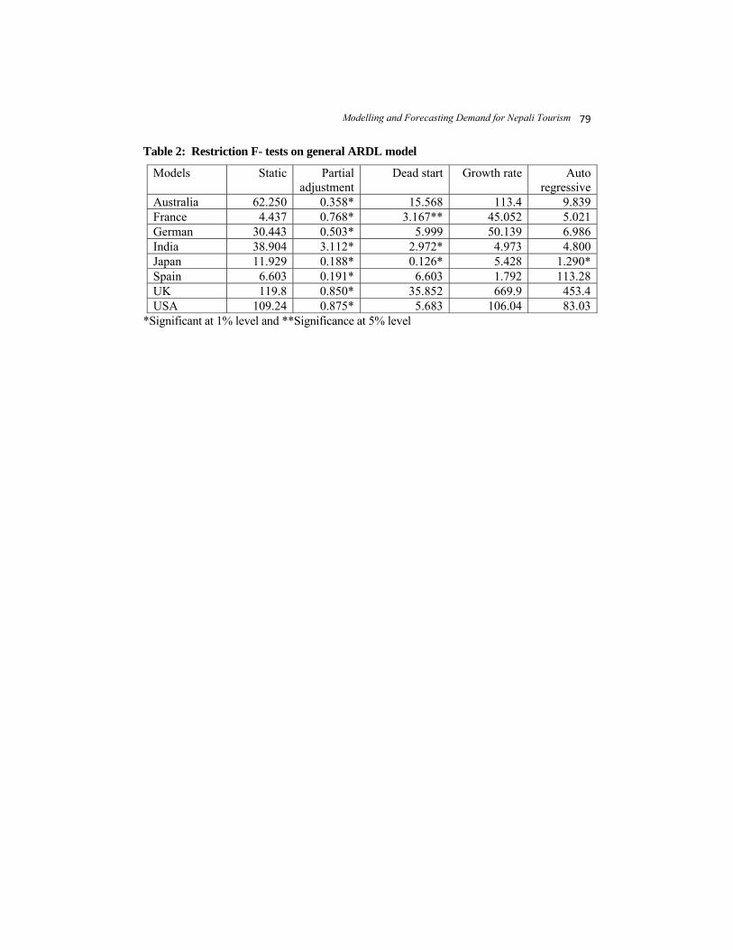
V. DIAGNOSTIC TESTS OF RESTRICTIVE MODELS The general ARDL includes all variables justified by the conceptual framework and economic theory and thus it is general model. However, all variables cannot be significant and appear with the correct sign. The reduced ARDL models can be derived from the general ARDL model by dropping statistically insignificant variables with an incorrect sign. So, this method filters the variables from the general ARDL equation estimation. By dropping out the variables with an incorrect sign and insignificant coefficients again the regressions are run on restrictive models. This reduces the number of independent variables from the ARDL and this type of ARDL is called as the reduced ARDL. With several rounds of trials and errors, one can come up with the correct form of the equation all with significant coefficients and the correct sign. Besides reduced model, there are a number of restricted models which are specific models such as static, partial adjustment, dead start, growth rate and autoregressive models. In this paper all these models are tried in the case of all major markets so as to find out to which models fit the best for the Nepali tourism data. However, only those models that pass the restriction F test on general ARDL are estimated. The results of the restriction F-tests on general model appear in table 2 (Annex). Almost all models are accepted at least at 5 percent level of restrictive F-tests and a very few ones are rejected. Some of the estimated models, although passed F-tests are found to be suffered from serial correlation and heteroskedasticity problems.
h
|Y-Y|=MAE tthT
1T=t
^
∑+
+
hy
y-y
t
tt=MAPEhT
1T=t
/^
100 ∑+
+
Modelling and Forecasting Demand for Nepali Tourism
69
The process to undertake restriction F-tests is as follows: After one estimates tourism demand from the general ARDL, various models can be tested imposing restrictions on ARDL equation given in (vii). For instance, for testing a partial adjustment model, by definition, one has to impose the restrictions (µ1 = φ1= α1= 0) on the ARDL equation. Similarly, for an autoregressive model, impose a zero restriction on all parameters except the lagged dependent variable, while a dead start model is estimated imposing zero restriction on all non-lagged parameters; and only intercept and lagged variables are included in this model and then regressed. Finally, a reduced ARDL model excludes all variables from the estimation of ARDL general model which are found statistically insignificant and appear with incorrect signs. The estimated residual from this model is used for the co-integration test of time series variables. Because, the regression of a non-stationary time series on another non-stationary time series may produce a spurious regression (Gujarati, 2007: 822). In other words, if two or more time series variables are not co-integrated, regression results are spurious. A regression that passes the check of co-integration produces non-spurious or stationary results, and the residual from such a regression is used as a right hand variable in the error correction mechanism. The residuals from the estimation of reduced ARDL, thus, are used for the estimation for Error correction model i.e., JML-Error Correction Mechanism (ECM2). In this mechanism, the first difference of left hand variables is regressed on a number of right hand side variables (first difference form). Besides, this type of error correction mechanism includes the one period lagged residual of co-integration regression as one of the right hand variables. Co-integration of two or more time series variables suggests that there is longrun relationship or equilibrium between them. Error correction mechanism is a means to reconciling the short behaviour of an economic variable with its longrun behaviour (Gujarati, 2007: 830). WB-Error Correction Mechanism (ECM1) , on the other, includes both first difference and lagged of right hand side variables together with the lagged left hand side variables; and finally the first difference of the left hand variable is regressed on first difference and lagged right hand variables and lagged left hand variable. All models presented in this paper are in double log form, because of the fact they perform better than other forms. Table 3 (Annex) presents Australia’s various demand models for Nepali tourism. Data on the Australian market fits only in the specific model such as partial adjustment model. Diagnostic checks on specific model’s performance show that partial adjustment model is better fit in the case of Australia. The tests confirm that lagged dependent variable, per capita income, own price, cross price, Dummy80, Dummy84, Dummy01 and Dummy05 are highly significant at 1% level and so these are the important variables for Australian arrivals into Nepal. The regression results from the reduced ARDL model confirm the results from the specific partial adjustment model. Income, price, cross price and dummy variables are found significant for the model. All specific models for Australia pass the diagnostic tests. Moreover, reduced ARDL passes the co-integration (CI) test. So, the error correction mechanism is estimated to see the

NRB ECONOMIC REVIEW
70
shortrun and longrun relationship between economic variables. The regresion results from error correction mechanism, ECM2, suggest that there is a fluctuation in number of visitor arrivals in the shortrun i.e., there exists shortrun deviation from the long term equilibrium level. As it is a short term phenomenon, it will restore up to its longrun equilibrium path. One period lagged residual variable appears with an expected negative sign in case of the Australian market and is statistically insignificant indicates that this shortrun fluctuation is insignificant so it will be adjusted quickly within this year. Most of the variables included in the model are found significant with the correct sign. Partial model shows a better fit since almost all visitors are found significant at the 1 percent level. In short, a number of variables such as lagged dependent variable, income, price, and cross price are responsible for attracting visitors from Australia. Among these, the word of mouth measured in terms of the lagged dependent variable is the most important variable. Moreover, the domestic and international events that affected adversely the tourist arrivals to Nepal from Australian market are captured by the dummies included the models. Table 4 (Annex) presents statistics on France’s demand for Nepali tourism, which shows that the data on France could fit on the specific models such as partial adjustment and dead start models. Almost all specific models failed the restrictive F tests. Only the reduced model passes the restriction test; this model is derived from the general ARDL model, dropping the variables with incorrect sign and insignificant t statistics. The reduced ARDL model passes all diagnostics checks and this model shows that lagged dependent, per capita income, and own price variables are found to be highly significant. More importantly, Dummy01 (September 11/Royal massacre) and Dummy 05(strike for republic) are found to have been key affecting factors in account of tourist arrivals from France. All variables including cross price variable appear with the expected sign and all variables except cross price are found statistically significant. Moreover, the CI test on residuals from reduced ARDL estimates confirms that time series dependent and independent variables are co-integrated to each other. ECM2 and ECM1 models are estimated to examine the linkage between shortrun deviation and longrun equilibrium. One period lagged residual variable appears with an expected negative sign and is found statistically significant at 1% level. This suggests that the shortrun swing will take more time to adjust to longrun equilibrium path. . Table 5 (Annex) displays regression results from German demand models for Nepali tourism. Germany remains another important market for Nepal from the very beginning. Almost all specific models fail the restriction tests but partial adjustment model passes the restriction F tests. In other words, all other specific models could not fit the tourist arrivals data from Germany. Lagged dependent variable, income, price, and cross price variables are the important variables for this market. Among the dummies, Dummy01 (September 11/Royal massacre) is found significant. ECM1 and ECM2 models are estimated because demand variables in the reduced model are found to be co-integrated. The important variables found statistically significant are lagged dependent and dummy01 variable for the error correction model. Table 6 (Annex) shows the regression results from the demand variables for India. Partial adjustment and dead start models pass the restrictive F-test. Also, almost all models pass the

Modelling and Forecasting Demand for Nepali Tourism
71
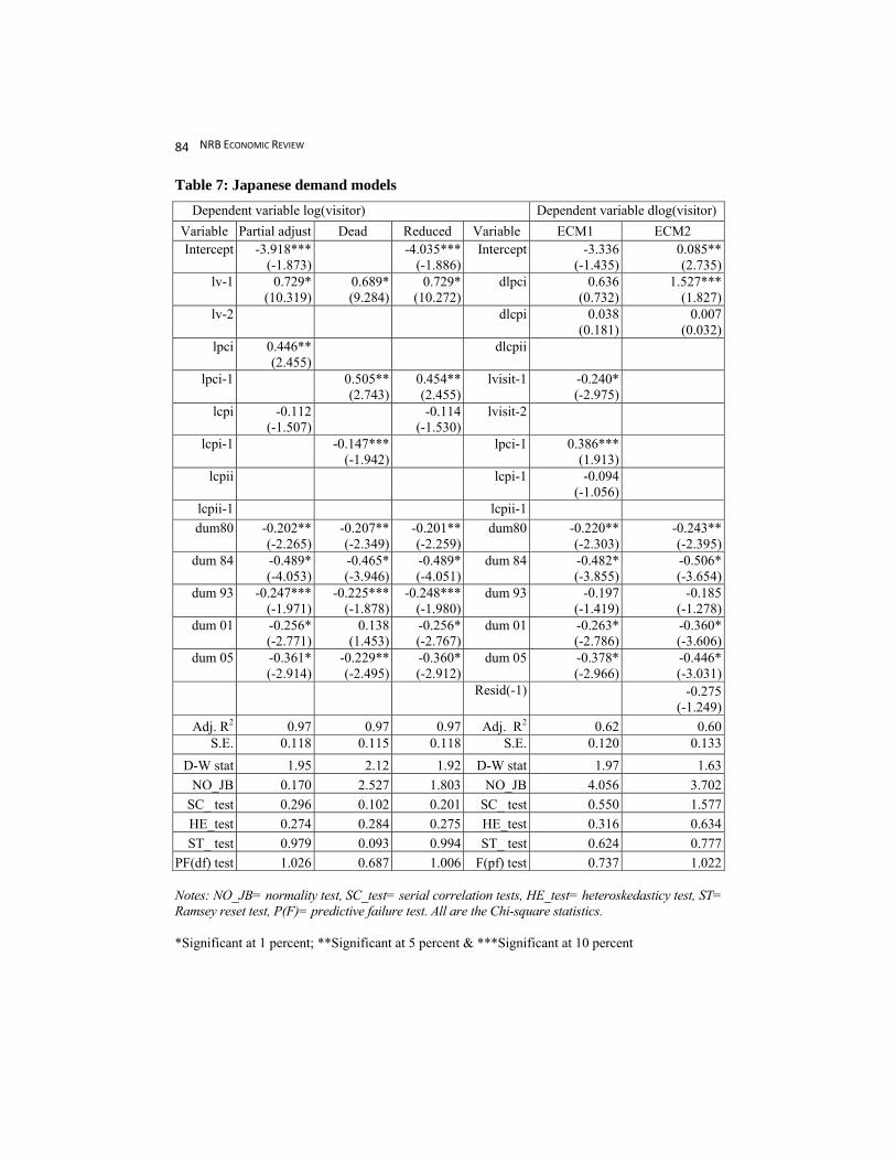
diagnostic tests. Key variables for Indian demand for Nepali tourism are the lagged dependent variable. India is a close neighbour with an open border to Nepal, and the purposes of the visit of most Indian visitors are pilgrim, official and business reasons. Indian tourists are mostly motivated by the positive information about Nepal from their friends and relatives or from newspapers or TVs. The income and price variables are found highly significant but both appear with incorrect sign. This can be indicative that a rise in the per capita income of Indian nationals diverts their destination from Nepal to relatively better/expensive destinations such as Thailand, Malaysia and Singapore. Among these Dummy89 and Dummy00 are most influential followed by Dum01 since those variables are found highly significant at the 1% level for all models considered for the Indian market. Lagged residual variable is found to be insignificant in ECM2 model but appears with the expected negative sign. Table 7 (Annex) presents the regression results from the demand variables for Japan. Japan is another prime market for Nepal. Specific models for Japan that pass F-tests are partial and dead models. Nepal is among the good choices for the Japanese, and favourite destinations in Nepal are Kathmandu and Pokhara. In case of Japan, the partial, dead start and reduced ARDL pass the restriction tests. Lagged dependent variable and per capita income are found as key demand variables in Japan Model. Besides, Dummy80, Dummy84, Dummy01and Dummy05 have reduced the number of arrivals from Japan significantly. Reduced ARDL estimation also confirms that above mentioned variables are vital for Japanese demand for Nepali tourism. CI tests on the residuals from the reduced model estimation show that times series data used in the model are co-integrated in a few cases. Thus, an error correction mechanism is applied using the lagged residual variable. Table 8 (Annex) shows regression results from Spain’s demand for Nepali tourism. This is another key and old tourism market for Nepal. The data on this market fit for partial adjustment specific model. This model passes the restriction test and the estimated statistics for this model are given in table 2. Accordingly, the lagged dependent variable, per capita income variable, own price variable, Dum80, Dum93 and Dum01 are found to be influential variables for Spain. The lagged residual variable in ECM2 model is also found statistically significant at the 1% level, indicating that short term fluctuation from the long term growth path is large, which takes the demand variable longer time to return to its equilibrium path. Specific model such as the partial adjustment model fit the UK demand data best, as this model passes the restriction test. As is presented by table 9 (Annex), the partial adjustment model shows that lagged dependent, per capita income, own price and cross price variables are highly significant. Dummy01 has created a severe adverse impact on the influx of UK visitors to Nepal. This is confirmed by partial, reduced, ECM1 and ECM2 models. So, the UK data fit the best on almost all models; and produce a relatively better result. Another important variable considered is the lagged dependent variable, which is found to be highly significant and has impacted positively on tourist arrivals from the UK, as priori expectation, lagged own price and lagged cross price variables have adversely and positively affected arrivals respectively. The lagged residual in ECM2 model appears with a negative sign but
NRB ECONOMIC REVIEW
72
statistically insignificant; implying that the shortrun fluctuation is small in magnitude and will soon return to the longrun equilibrium level. Data on the USA market fit best on specific models (Annex Table 10) such as the partial adjustment model. Functional forms of all specific models shown in the table have passed restrictive F-tests. Diagnostic tests on different models indicate that specific models on USA data perform better as compared to other markets. A number of variables considered in the models are found to be significant mostly at 1% level. Income, own price and cross price variables are found to be significant. Likewise, lagged forms of own and cross price variables are highly significant. But the lagged of income variable is found as insignificant. This implies that there exists a short-run (but not long-run) behavioural impact of income variable on tourist arrivals from the USA. The influential events that affected tourist arrivals from this market are Dummy74 Dummy80 Dummy84, Dummy93, Dummy01 and Dummy05. All dummies are found significant at 1% level. Almost all ECM models, except French and Spanish markets show that the lagged residual variable (from co-integrating equation, which exhibits the longrun equilibrium) is found to be insignificant statistically confirms the existence of shortrun disequilibrium in the market. Furthermore, almost all lagged residual variables appear statistically insignificant indicate that deviation in the shortrun is very short and disequilibrium will be corrected and longrun equilibrium will be restored within very short span of time. However, in the cases of France and Spain shortrun disequilibrium is found statistically significant suggests that this will take more time to restore to equilibrium path. In addition to these findings, given the CI relationship being assured by statistical tests, long-run and short-run tourism demand elasticity can be calculated from the double log form of CI equation and the ECM respectively. With regard to the income elasticity, lower coefficient of income variable in ECMs than those in the CI models implies that income is influential variable in the longrun compare to the shortrun. It is, to some extent, consistent with Friedman’s permanent income hypothesis, which claims that consumption depends on people’s expectation of future earnings over a considerable period of time. Several empirical studies show that the values of both the income and own-price elasticity in the longrun are greater than their short-run counterparts, suggesting that tourists are more sensitive to income and price changes in the longrun than in the shortrun. These findings are in line with demand theory and other empirical studies carried out for other countries. A significant substitution effect indicates the presence of the strong competitors; and different degrees of substitution between the competing destinations show their competitive positions in the tourism markets. The sign of cross price variable indicates that India is a competitor for Nepal in relation to many tourism markets and complement in a few market cases. In view of this, it is necessary to adopt appropriate strategies based on the specific attributes the destinations possess. Nepal has to focus on differentiated markets segments to make optimum use of own competitive and comparative advantages. The forecasting power varies across different forecasting horizons. In general, uncertainty increases with the longer forecasting time horizon for the specific models; and so, the less accurate is the prediction. For this reason, predictive F-test or P(F) test has been
Modelling and Forecasting Demand for Nepali Tourism
73
performed for the period 2006 to 2009 to examine the predictive power of all models considered for specific markets. In short, the lagged dependent variable is the single most important variable that has influenced positively to the tourist arrivals from all tourism markets. It underscores the predominant role of the ‘word of mouth’ in the current status of tourism development. Nepal is well-known for her smiling people, natural beauty, mountains and landscapes that attract and motivate tourists overwhelmingly for trekking. A significant number of the repeated visitors substantiate that lagged the dependent variable is extremely important to the country. It is important to note that their likeness and willingness to repeat visits for self also influence their friends and family members; and their recommendations to others to visit Nepal motivate and generate more tourists for the country. They should be recognized as the best friends of Nepal and honoured as unpaid promoters of Nepali tourism in international tourism markets. This is all related to the lagged dependent variable. Dummy01 and Dummy05 have largely affected tourist arrivals in the country. Besides, per capita incomes of the visitors has positively affected tourist arrivals into Nepal while an increase in own price (rcpi), a decrease in cross price (i.e., tourism price in substitute destination) and dummy variables, such as, September 11, oil price hike and demolition of the Barbari mosque have affected tourist arrivals adversely.
VI. FORECASTING TOURISM DEMAND The number of tourist arrivals from eight major markets is forecated for 2010-2020 using multivariate regression models that are considered the appropriate based on the diagnostic tests widely used by econometricians. For this purpose, various independent variables are forecasted using Hodrick-Prescot Filter, a smoothing method. Table 11 (Annex) presents forecasting statistics of the partial adjustment models for eight tourism markets of Nepal. Almost all countries considered pass the restriction tests for partial adjustment models and for this reason all markets are presented in the table. Forecasting statistics are supposed to exhibit the performance of the specific model. On this count, the forecast statistics presented in the table for the partial adjustment model exhibit perfect fitness of the data and so, the estimated coefficients for demand variables using this model are reliable. Bias and variance proportions of Theil U exhibit excellent results and confirm the better forecasting power of the partial adjustment models for all markets. Comparatively, the variance proportion is rather small for Australia, UK, USA, India and Germany. MAPE is overwhelmingly used in forecast statistics and in our case all MAPE statistics for partial adjustment models also show the good predictive power of the models. Comparatively MAPE statistics for Spain is larger as compare to those for other markets. In terms of MAE statistics also the adjustment models for all market perform with better statistics. Comparatively again, the UK, USA, India, and Australia perform better than others giving relatively smaller values. RMSE is another important forecasting statistic to examine the

NRB ECONOMIC REVIEW
74
predictive power of the models. On this statistics count also, the partial adjustment model shows a better fit. Table 12 (Annex) presents the magnitudes of the forecasting errors for the dead start regression model. Forecast statistics in French, Indian and Japanese markets are presented in the table because of the fact only these three markets could pass the restrictive tests (see table 6). All types of forecasting errors are smaller, which exhibit an excellent performance of the dead start model for all markets. MAPE statistics for India is less than one. The RMSE and MAE statistics in the case of these markets are found less than one. Theil U is close to zero for all markets for which the bias component is zero and almost the same is the variance component. These all indicate the good fitness of the data for this specific model. Table 13 (Annex) presents the magnitudes of the forecasting errors for the reduced regression model for all eight major tourism markets considered in the study. Forecast statistics for almost all markets except Spanish show smaller predictive errors which implies that the ARDL model fits well for Nepali tourism data. Table 14 (Annex) presents the magnitudes of forecasting errors for Wickens-Bruesch Error Correction Mechanism. Forecast statistics for all markets are presented in the table. This mechanism shows MAPE statistics to be higher for all markets. The rest of the statistics are comparable with specific models such as partial adjustment, dead start and reduced ARDL models. Table 15 (Annex) presents the magnitudes of the forecasting errors for Johansen Maximum Likelihood ECM. Forecast statistics except MAPE for almost all markets presented in the table are comparable with those from other models. Across the markets, MAPE for Japan, Australia, USA, Spain, India and the UK are relatively higher as compare to those for other markets. However, this statistics for France is surprisingly low as compare to others. The statistics shown in tables 11 to 15 measure the forecasting performance of the specific models. In almost all equations, bias and variance proportions of Theil-U are reported small indicating that the models considered are good enough to forecast the future demand behaviour of the tourism in the country. In addition, the variance proportion is close to one for most of the models. Table 16 (Annex) displays the forecasted growth rates of tourist arrivals from major eight markets for 2010 to 2020 using best performed models. The forecasted number of tourists is compared with the actual average annual growth rates for three periods. The forecasted growth rates for various markets are found very close to actual growth rates for the period 2006 to 2010 which are used as a benchmark for the analysis of the forecasted growth rates. The forecasted growth rates from ECM2 for Australia, France, UK and USA are comparable with the actual growth rates for the period 2006 to 2010, while those from reduced model for Germany and India and dead start model for Japan are comparable with the same period. Table 17 (Annex) presented the forecasted number of tourist arrivals in Nepal from major eight markets during 2010 to 2020. The forecasted number of the tourist arrivals gives the
Modelling and Forecasting Demand for Nepali Tourism
75
growth rates shown in the last row of table 16, which is comparable with the growth rates for the last decade (2000 to 2010). It is based on the assumption that past trend will continue for the next eleven years. The projected figures of tourist arrivals from the major markets can provide a guideline for the policy makers.
VII. CONCLUSION AND POLICY IMPLICATION The demand for Nepali tourism is a part of world tourism demand. Moreover, it is a small fraction of the South Asian tourism demand. The global demand for tourism has grown with the rapid growth of economies in the west. Travelling becomes one of the items in consumers’ consumption basket. Data on tourist arrivals from all major markets are found to be fitted into the given models. This study confirms that the demand for Nepal is the composite function of almost all variables considered. Of these, the lagged dependent variable, income, own price and dummies like Dummy89, Dummy01 and Dummy05 are found highly significant. This indicates that tourism demand in Nepal is highly governed by short run social and political events within the country and in en route countries like India and South East Asia. In addition to these, words of mouth, income, and price variables are influencial variables in determing the demand for Nepali tourism. Among the major eight markets, majority are found to be at longrun equilibrium path since the shortrun fluctuations are found the least influencial. Only in two markets -France and Spain -such fluctuations are found to be significant in the shortrun. This indicates that it will take longer time to adjust in the longrun equilibrium path in case of these markets. The most important policy implication is the words of mouth which can prove to be an important marketing and promotion strategy. This can be done through the up-gradation of the tourist products for the better image of the destination. Good words of mouth can result in the increased influx of repeated visitors and their recommended number of first time visitors. Furthermore, it also manifests that there is no such urgent need for spending scarce resource on the tourism advertisement through the international media such as CNN and BBC. Another important policy implication is that India as a destination is a substitute destination to Nepal. It can be seen that majority of visitors from overseas come to Nepal independently rather than in conjunction to India. Thus, Nepal has to focus on differentiated market segments to make optimum use of the competitive and comparative advantages. The estimated higher coefficients for the longrun income, own price and cross elasticity of demand as compared to those of shortrun clearly indicates the higher elasticities for the longrun ones. Now, it can be concluded that although income, price and cross price variables are important ones, they are less important in the shortrun. The relatively higher elasticity of the lagged dependent variable and dummies in the ECM model is indicative that the words of mouth and political stability in the country as well as in the region are more relevant variables implies that they influence much to the shortrun tourist arrivals in Nepal. Note that

NRB ECONOMIC REVIEW
76
both in shortrun and longrun words of mouth variable is the most influential variable for all major markets. In majority cases, statistically insignificant coefficient of the lagged of residuals in ECM2 models suggest that there are minor departure from the path of longrun equilibrium and thus tourism demand would adjust to the changes in its determinants within the same period. Only in a few other cases it would take more time to adjust. The best performed models are used for forecasting the growth rates of tourist arrivals from the eight major markets for 2010 to 2020. The forecasted growth rates of tourist arrivals are compared with the actual average annual growth rates for three periods, 2006-10, 2005-2009, and 2000-10. Of these the forecasted growth rates are found very close to 2006 to 2010.
*****
REFERENCES Becker, Gary S. 1965. "A Theory of the Allocation of Time." The Economic Journal 75: 493-517.
Macmillan Limited, London.
Burger,Veit. 1978. The Economic Impact of the Tourism in Nepal: An Input Output Analysis. Ph.D dissertation. Cornell University, Ann Arbor, University Micro films, Michigan.
Bwire, B.M. 1987. International Tourist Flows to Keyna. Master in Economics Thesis. Department of Economics. Dalhousie University. Halifax Canada.
English, E. Philip. 1986. The Great Escape: an examination of North-South Tourism. The North South Institute, Ottawa.
Gujrati,D.N. 2007. Basic Econometrics. McGraw-Hill Publishing Company, New York.
Hendry, D.F. 1995. Dynamic Econometrics. Oxford University Press, Oxford.
Holloway, J Christopher (1998): The Business of Tourism. Addison Longman Limited, London, UK.
IMF. Various issues. International Financial Statistics Yearbook. International Monetary Fund, Washinton DC.
Johnson, Peter and John Ashworth. 1990. “Modelling Tourism Demand: A Summary Review.” Leisure Studies 9(1):145-151.
Kaul, V. 1994. Tourism and Economy. Har-Anand Publications, New Delhi.
Kmenta,Jan. 1971. Elements of Econometrics. Macmillan Publishing Co.,Inc., New York.
Krause and Jude (1973), "Latin America", in Econometric Models and Economic Impact. Singapore University Press, Ottawa.
Mathematica (1970): "The Visitors Industry and Hawaii's Economy: A Cost Benefits Analysis." in Mathematica Princeton, New Jersey.
Mitchell, F. (1971): The Economic Value of Tourism In Kenya. Ph.D dissertation, University of California.

Modelling and Forecasting Demand for Nepali Tourism
77
Morley, Clive. 1991. “Modelling International Tourism Demand: Model Specification and Structure.” Journal of Travel Research 30: 40-44.
MoTCA.Various issues. Nepal Tourism Statistics. GoN, Ministry of Tourism and Civil Aviation, Kathmandu.
NRB.1989. Income and Employment Generation from Tourism in Nepal. Nepal Rastra Bank, Kathmandu, Nepal.
Paudyal, Shoora B. 2013. Economic Analysis of SAARC Tourism: Analysis of Demand and Supply. LAP Lambert Academic Publishing AG & Co., Germany.
------------. 2012. Tourism in Nepal: Economic Perspectives. Buddha Academic Publishers and Distributors Pvt. Ltd, Kathmandu, Nepal.
--------- .1998. “International Demand for Tourism in Nepal.” Economic Review 10. Nepal Rastra Bank, Kathmandu.
--------- .1993. An Econometric Model of Demand for Tourism in Nepal, MA thesis. Department of Economics. Dalhousie University, Halifax, Canada.
Pindyck, R.C. and Daniel L. Rubinfeld.1991. Econometric Models and Economic Forecasts. McGraw-Hill Inc, New York.
Pye, Elwood A. and Tzong-biau Lin (1983). Tourism in Asia: The Economic Impact. Singapore University Press, Ottawa.
QMS. 2004. Eviews 5 User’s Guide. Quantitative Micro Software, LLC, Irvine CA.
Song, H. Aiyan, Stephen F. Witt and Gang Li. 2003. “Modelling and forecasting the demand for Thai tourism.” Journal Tourism Economics 9(4), 363-387.
Smeral, Egon. 1988. “Tourism Demand, Economic Theory and Econometrics: An Integrated Approach.” Journal of Travel Research 26.
Smith, Valene L. 1977. Hosts and Guests: the Anthropology of Tourism. University of Pennsylvania Press Inc., USA.
Studenmund, AH and Henry J. Cassidy.1987. Using Econometrics, a Practical Guide. Little Brown and Company Boston, Toronto.
Witt, Stephen F. and Christine A. Witt. 1992. Modelling and Forecasting Demand in Tourism. Academic Press Ltd, U.K.
Woo, Art zen . 1992. Canada’s International Tourism Exports: An Econometric Study of the Determinants of Demand. MA thesis. Economics Department, Dalhousie University. Halifax Canada.

NRB ECONOMIC REVIEW
78
Annex
Table 1: ARDL general model for selected tourist generating markets
Dependent variable (log of visitors) Variable Australia France Germany India Japan Spain UK USA
C -28.288* (-5.748)
-18.731*(-4.086)
-34.652*(-5.455)
2.686*(3.252)
-5.324(-1.385)
-25.962*(-3.596)
-13.150* (-3.833)
-7.506*(-2.831)
lv-1 0.707* (6.313)
0.381**(2.374)
0.945*(6.162)
0.765*(10.633)
0.662*(6.741)
0.267**(2.474)
0.860* (6.000)
0.899*(18.314)
lv-2 0.139
(1.212) 0.030
(0.239)-0.153
(-0.974)0.624
(0.305)0.456*(5.086)
0.015 (0.113)
lpci 5.337
(0.857) 8.755
(0.761)3.705*(3.652)
-13.117**(-2.433)
-0.0426(-0.021)
-7.082(-0.582)
15.310 (1.506)
2.384*(3.519)
lpci-1 -1.816
(-0.291) -6.256
(-0.543)0.711
(0.969)12.816**
(2.374)-0.276
(-0.556)9.209
(0.759)-12.955 (-1.292)
-0.653(-1.123)
lcpi -2.788* (-6.801)
-1.0479**(-2.147)
-0.588***(-1.946871)
-0.224(-0.607)
0.044(0.101)
-1.542*(-2.967)
-2.433* (-4.579)
-0.430(-1.461)
lcpi-1 0.054
(0.173) -0.483
(-1.230)0.004
(0.012)0.606
(1.585)0.246
(0.527)0.127
(0.247)0.380
(0.994) -0.037
(-0.135)
Lcpii 0.854** (2.479)
0.328(0.698)
-0.159(-0.465)
-0.172(-0.449)
0.197(0.595)
0.814** (2.519)
0.249(1.086)
lcpii-1 -0.243
(-0.795) 0.195
(0.501)-0.893**(-2.725)
-5.324(-1.385)
-0.045(-0.112)
-0.185 (-0.735)
0.199(1.083)
dum74 -0.080
(-0.542) -0.237*(-4.364)
dum80 -0.276** (-2.342)
-0.125(-0.851)
-0.124(-0.743)
-0.188(-1.839
-0.661**(-2.276)
-0.027 (-0.192)
-0.190*(-3.461)
dum84 -0.724* (-4.615)
-0.222(-1.559)
-0.144(-1.225)
-0.493*(-3.662)
-0.236(-1.146)
-0.117 (-0.960)
dum89 -0.629*(-5.653)
dum91 -0.229
(-1.464) 0.002
(0.015)
dum93 -0.208
(-1.394)-0.214
(-1.459)-0.342
(-1.625) -0.111*(-3.023)
dum98 0.129
(1.442)0.101
(0.858)-0.227
(-1.34d)0.155
(1.445)0.007
(0.029)0.078
(0.848)
dum00 -0.414*(-3.559)
dum01 -0.415* (-3.267)
-0.253**(-2.252)
-0.119(-1.021)
-0.498*(-4.487)
-0.226**(-2.259)
-0.546**(-2.050)
-0.522** (-4.234)
-0.504*(-2.865)
dum05 -0.462* (-2.820)
-0.437*(-3.097)
-0.190(-1.182)
-0.353**(-2.601)
-0.331(-1.205)
-0.035 (-0.263)
-0.270*(-3.681)
dum08
0.014(0.042)
Adj. R2 0.98 0.90 0.96 0.96 0.97 0.970 0.98 0.96S.E. 0.147 0.125 150 104 0.123 0.246 0.115 0.106D-W stat 1.74 2.49 2.11 1.88 2.12 1.68 2.077 2.28 F-stat 174 26.31 88.19 98.31 98.35 108.2 208.1 86.49F(pf) 0.96 2.59*** 1.91 0.079 0.608 0.670 2.021 2.033N
46(1964-09) 40(1970-
09)44(1966-
09)35(1975-
09)40(1970-
09)43(1967-
09)47(1963-09) 47(1963-09)
*Significant at 1 percent; **Significant at 5 percent & ***Significant at 10 percent
Modelling and Forecasting Demand for Nepali Tourism
79
Table 2: Restriction F- tests on general ARDL model
Models Static Partial adjustment
Dead start Growth rate Auto regressive
Australia 62.250 0.358* 15.568 113.4 9.839France 4.437 0.768* 3.167** 45.052 5.021German 30.443 0.503* 5.999 50.139 6.986India 38.904 3.112* 2.972* 4.973 4.800Japan 11.929 0.188* 0.126* 5.428 1.290*Spain 6.603 0.191* 6.603 1.792 113.28UK 119.8 0.850* 35.852 669.9 453.4USA 109.24 0.875* 5.683 106.04 83.03
*Significant at 1% level and **Significance at 5% level

NRB ECONOMIC REVIEW
80
Table 3: Australian demand models
Dependent variable log(visitor) Dependent variable dlog(visitor)Variable Partial adjust Reduced Variable ECM1 ECM2Intercept -28.256*
(-5.967) -27.971*(-5.813)
Intercept 9.044***(1.819)
0.105**(2.068)
lv-1 0.704* (6.380)
0.688(6.223)*
dlpci 0.949(0.848)
2.077(1.239)
lv-2 0.145 (1.294)
0.161(0.160)
dlcpi 0.184927(0.458)
-0.350(-1.288)
lpci 3.500* (6.170)
dlcpii 0.905**(2.645)
0.434(1.302)
lpci-1
3.454*(6.012)
lvisit-1 -0.277**(-2.468)
lcpi -2.760* (-7.328)
-2.707*(-7.168)
lvisit-2 0.132(1.151)
lcpi-1
lpci-1 -1.037***(-1.752)
lcpii 0.739* (2.786)
0.722**(2.675)
lpi-1 0.208(0.495)
lcpii-1 0.144 (1.294)
lpii-1 0.686**(2.341)
dum80 -0.254** (-2.217)
-0.254**(0.036)
dum80 -0.253**(-2.141)
-0.246*(-4.398)
dum84 -0.699* (-4.589)
-0.686*(-4.444)
dum84 -0.744*(-4.624)
-0.844*(-8.033)
dum01 -0.439* (-3.603)
-0.439*(-3.561)
dum02 -0.420*(-3.289)
-0.428*(-5.924)
dum05 -0.471* (-2.972)
-0.472(-2.940)*
dum05 -0.454*(-2.754)
-0.439*(-8.699)
Resid(-1) -0.044(-0.194)
Adj. R2 0.98 0.98 Adj. R2 0.65 0.39S.E. 0.145 0.147 S.E. 0.148 0.187
D-W stat 1.70 1.70 D-W stat 1.70 0.974NO_JB 5.66*** 3.32 NO_JB 8.27** 5.56***
SC_ test 1.01 1.07 SC_ test 1.07 19.03*HE_test 1.07 1.06 HE_test 1.20 0.82ST_ test 1.61 1.34 ST_ test 1.79 0.98P(F) test 0.93 0.96 0.97 0.32
Notes: NO_JB= normality test, SC_test= serial correlation tests, HE_test= heteroskedasticy test, ST= Ramsey reset test, P(F)= predictive failure test. All are the Chi-square statistics. *Significant at 1 percent; **Significant at 5 percent & ***Significant at 10 percent

Modelling and Forecasting Demand for Nepali Tourism
81
Table 4: French demand models Dependent variable log(visitor) Dependent variable dlog(visitor)
Variable Partial adjust Dead Reduced Variable ECM1 ECM2 Intercept -18.922*
(-4.459) -10.311*(-2.893)
-17.323*(-4.273)
Intercept 8.509* (3.286)
0.075* (2.969)
lv-1 0.458* (3.191)
0.073(0.655)
0.443*(2.890)
dlpci 0.381 (0.268)
0.387 (0.364)
lv-2 0.063 (0.526)
0.291**(2.672)
0.096(0.813)
dlcpi 1.016** (2.627)
-0.388** (-2.672)
lpci 2.486* (5.373)
dlcpii -0.613 (-1.481)
lpci-1
1.515371*(3.957)
2.325*(5.195)
lvisit-1 -0.513* (-4.546)
lpi -1.242* (-3.364)
-0.985*(-3.892)
lvisit-2
lcpi-1
-0.899**(-2.424)
lpci-1 -0.730* (-3.395)
lcpii 0.306 (1.074)
lcpi-1 0.567 (1.616)
lcpii-1
0.352361(1.107)
0.097(0.564)
lcpii-1 -0.332 (-1.022)
dum80 dum80 dum84 -0.245***
(-1.795) -0.247
(-1.579)-0.242***
(-1.735)dum84 -0.227
(-1.631) -0.338*
(-10.364) dum93 -0.263***
(-1.823) -0.133
(-0.854)-0.300**(-2.120)
dum93 -0.239 (-1.557)
-0.300* (-7.458)
dum01 -0.307* (-2.899)
-0.369*(-3.046)
-0.318*(-2.903)
dum01 -0.274** (-2.658)
-0.330 (-1.476)
dum05 -0.409* (-3.064)
-0.479*(-3.030)
-0.391*(-2.890)
dum05 -0.460* (-3.325)
-0.346* (-13.861)
Resid(-1) -0.644* (-3.360)
Adj. R2 0.91 0.87 90 Adj. R2 0.57 0.51 S.E. 0.124 0.142 0.127 S.E. 0.124 0.128
D-W stat 2.210 2.00 2.06 D-W stat 2.42 1.81 F-stat 44.02 11.92 41.95 F-stat 5.85 6.67
NO_JB 1.44 0.249 1.21 NO_JB 1.67 0.17 SC_ test 1.32 0.912 0.76 SC_ test 1.70 2.03 HE_test 1.127 1.686 1.08 HE_test 0.54 4.5* ST_ test 0.05 3.595 0.103 ST_ test 1.12 0.20
PF(df) test 1.39 0.87 1.40 F(pf) test 1.46 0.40 Notes: NO_JB= normality test, SC_test= serial correlation tests, HE_test= heteroskedasticy test, ST= Ramsey reset test, P(F)= predictive failure test. All are the Chi-square statistics. *Significant at 1 percent; **Significant at 5 percent & ***Significant at 10 percent

NRB ECONOMIC REVIEW
82
Table 5: German demand models
Dependent variable log(visitor) Dependent variable dlog(visitor) Variable Partial adjust Reduced Variable ECM1 ECM2Intercept -28.154*
(-4.691) -36.198*(-6.353)
Intercept 0.917(0.308)
0.101*(3.224)
lv-1 0.831* (5.466)
0.991(6.949)*
dlpci 0.762(1.062)
-0.589(-0.891)
lv-2 0.058 (0.420)
-0.204(-1.512)
dlcpi 0.309(1.170)
-0.268(-0.681)
lpci 3.590* (5.173)
3.733*(4.000)
dlcpii -0.207(-0.728)
-0.037(-0.093)
lpci-1
0.876(1.255)
lvisit-1 -0.0278(-0.311)
lcpi -0.308 (-1.226)
-0.654*(-3.557)
lvisit-2 -0.130**(-2.137)
lcpi-1
lpci-1 0.036(0.109)
lcpii -0.894* (-3.270)
lcpi-1
lcpii-1
-1.072770*(-5.267245)
lcpii-1
dum80 dum80dum84 dum84dum93 dum93dum01 -0.271**
(-2.455) dum01 -0.163
(-1.662)-0.307*(-2.726)
dum05 -0.158 (-0.907)
dum05 -0.172(-0.910)
Resid(-1) -0.029(-0.141)
Adj. R2 0.95 0.96 Adj. R2 0.41 0.06S.E. 0.165 0.149 S.E. 0.150 0.183
D-W stat 2.00 1.98 D-W stat 1.948 1.571NO_JB 0.563 2.155 NO_JB 2.787 0.405
SC_ test 2.83** 1.191 SC_ test 1.168 2.447HE_test 1.079 1.259 HE_test 0.787 0.930ST_ test 1.838 1.209 ST_ test 0.67 0.148
PF(df) test 1.708 1.995 F(pf) test 1.90 1.323 Notes: NO_JB= normality test, SC_test= serial correlation tests, HE_test= heteroskedasticy test, ST= Ramsey reset test, P(F)= predictive failure test. All are the Chi-square statistics. *Significant at 1 percent; **Significant at 5 percent & ***Significant at 10 percent

Modelling and Forecasting Demand for Nepali Tourism
83
Table 6: Indian demand models
Dependent variable log(visitor) Dependent variable dlog(visitor)
Variable Partial adjust
Dead start Reduced Variable ECM1 ECM2
Intercept 3.336* (3.979)
3.297*(4.064)
3.330*(3.941)
Intercept 3.393* (3.808)
0.104* (3.335)
lv-1 0.751* (9.774)
0.763*(10.642)
0.752*(9.756)
dlpci 0.062 (0.329)
-0.109 (-0.513)
lpci -0.298* (-3.331)
dlcpi 0.003 (0.006)
-0.162 (-0.360)
lci-1
-0.317*(-3.389)
-0.296*(-3.288)
lvisit-1 -0.243* (-3.041)
Lcpi 0.305** (2.767)
0.301**(2.730)
lpci-1 -0.325* (-3.213)
lcpi-1
0.313*(2.833)
lcpi-1 0.316** (2.742)
-0.228 (-0.935)
dum89 -0.661* (-5.580)
-0.665*(-5.639)
-0.661*(-5.559)
dum89 -0.664* (-5.427)
-0.601* (-4.199)
dum98 0.078 (0.662)
0.084*(0.481)
0.085(0.715)
dum98 0.088 (0.720)
0.001 (0.005)
dum00 -0.359* (-3.024)
-0.391*(-3.327)
-0.360*(-3.017)
dum00 -0.386* (-3.006)
-0.489* (-3.370)
dum01 -0.459* (-3.976)
-0.483*(-4.172)
-0.459*(-3.963)
dum01 -0.481* (-3.908)
-0.503* (-3.483)
Resid(-1) -0.228 (-0.935)
Adj. R2 95 0.95 0.95 Adj. R2 0.65 0.50 S.E. 0.112 0.111 0.112 S.E. 0.115 0.139
D-W stat 1.884 1.94 1.887 D-W stat 1.878 1.513 NO_JB 4.505 3.983 4.312 NO_JB 4.158 1.997
SC_ test 0.062 0.075 0.064 SC_ test 0.081 3.44** HE_test 0.401 0.498 0.404 HE_test 0.495 1.297 ST_ test 0.273 2.274 0.271 ST_ test 0.259 2.292
PF(df) test 0.121 0.056 0.120 F(pf) test 0.050 0.515
Notes: NO_JB= normality test, SC_test= serial correlation tests, HE_test= heteroskedasticy test, ST= Ramsey reset test, P(F)= predictive failure test. All are the Chi-square statistics. *Significant at 1 percent; **Significant at 5 percent & ***Significant at 10 percent
NRB ECONOMIC REVIEW
84
Table 7: Japanese demand models
Dependent variable log(visitor) Dependent variable dlog(visitor) Variable Partial adjust Dead Reduced Variable ECM1 ECM2 Intercept -3.918***
(-1.873) -4.035***
(-1.886)Intercept -3.336
(-1.435)0.085**(2.735)
lv-1 0.729* (10.319)
0.689*(9.284)
0.729*(10.272)
dlpci 0.636(0.732)
1.527***(1.827)
lv-2
dlcpi 0.038(0.181)
0.007(0.032)
lpci 0.446** (2.455)
dlcpii
lpci-1
0.505**(2.743)
0.454**(2.455)
lvisit-1 -0.240*(-2.975)
lcpi -0.112 (-1.507)
-0.114(-1.530)
lvisit-2
lcpi-1
-0.147***(-1.942)
lpci-1 0.386***(1.913)
lcpii
lcpi-1 -0.094(-1.056)
lcpii-1 lcpii-1 dum80 -0.202**
(-2.265) -0.207**(-2.349)
-0.201**(-2.259)
dum80 -0.220**(-2.303)
-0.243**(-2.395)
dum 84 -0.489* (-4.053)
-0.465*(-3.946)
-0.489*(-4.051)
dum 84 -0.482*(-3.855)
-0.506*(-3.654)
dum 93 -0.247*** (-1.971)
-0.225***(-1.878)
-0.248***(-1.980)
dum 93 -0.197(-1.419)
-0.185(-1.278)
dum 01 -0.256* (-2.771)
0.138(1.453)
-0.256*(-2.767)
dum 01 -0.263*(-2.786)
-0.360*(-3.606)
dum 05 -0.361* (-2.914)
-0.229**(-2.495)
-0.360*(-2.912)
dum 05 -0.378*(-2.966)
-0.446*(-3.031)
Resid(-1) -0.275(-1.249)
Adj. R2 0.97 0.97 0.97 Adj. R2 0.62 0.60S.E. 0.118 0.115 0.118 S.E. 0.120 0.133
D-W stat 1.95 2.12 1.92 D-W stat 1.97 1.63NO_JB 0.170 2.527 1.803 NO_JB 4.056 3.702
SC_ test 0.296 0.102 0.201 SC_ test 0.550 1.577HE_test 0.274 0.284 0.275 HE_test 0.316 0.634ST_ test 0.979 0.093 0.994 ST_ test 0.624 0.777
PF(df) test 1.026 0.687 1.006 F(pf) test 0.737 1.022 Notes: NO_JB= normality test, SC_test= serial correlation tests, HE_test= heteroskedasticy test, ST= Ramsey reset test, P(F)= predictive failure test. All are the Chi-square statistics. *Significant at 1 percent; **Significant at 5 percent & ***Significant at 10 percent

Modelling and Forecasting Demand for Nepali Tourism
85
Table 8: Spanish demand models
Dependent variable log(visitor) Dependent variable dlog(visitor) Variable Partial adjust Reduced Variable ECM1 ECM2 Intercept -27.358*
(-4.774) -25.867*(-4.581)
Intercept 38.706*(6.383)
0.149*(3.298)
lv-1 0.215** (2.408)
0.216**(2.387)
dlpci -0.385(-0.256)
1.141(0.719)
lv-2 0.411* (5.329)
0.425*(5.554)
dlcpi 1.853*(3.969)
0.665**(2.681)
lpci 2.261* (5.142)
dlcpii -0.104(-0.654)
lpci-1
2.148*(4.958)
lvisit-1 -0.787*(-7.887)
lcpi -1.435* (-4.737)
-1.410*(-4.628)
lvisit-2 0.410*(4.833)
lcpi-1
lpci-1 -2.912*(-6.242)
lcpii
lcpi-1 1.872*(5.474)
dum80 -0.588** (-2.369)
-0.603**(-2.411)
dum80 -0.583**(-2.070)
-0.658*(-10.376)
dum 93 -0.354*** (-2.033)
-0.342***(-1.951)
dum 93 -0.306(-1.547)
-0.272*(4.521)
dum 01 -0.607** (-3.367)
-0.579*(-3.197)
dum 01 -0.336(-1.658)
-0.496*(-3.663)
dum 05 -0.332 (-1.347)
dum 05
0.454*(10.006)
Resid(-1) -0.631*(-6.055)
Adj. R2 0.97 0.97 Adj. R2 0.72 0.37S.E. 0.233 0.235 S.E. 0.249 0.276
D-W stat 1.569 1.569 D-W stat 1.618 1.809NO_JB 1.00 0.239 NO_JB 0.083 0.354
SC_ test 2.143 2.861 SC_ test 3.277 0.094HE_test 0.565 0.621 HE_test 0.932 0.513ST_ test 1.276 1.189 ST_ test 6.848 3.287
PF(df) test 0.614 0.671 F(pf) test 0.539 0.170 Notes: NO_JB= normality test, SC_test= serial correlation tests, HE_test= heteroskedasticy test, ST= Ramsey reset test, P(F)= predictive failure test. All are the Chi-square statistics. *Significant at 1 percent; **Significant at 5 percent & ***Significant at 10 percent

NRB ECONOMIC REVIEW
86
Table 9: UK demand models
Dependent variable log(visitor) Dependent variable dlog(visitor) Variable Partial adjust Reduced Variable ECM1 ECM2
Intercept -11.086* (-3.831)
-17.094*(-15.102)
Intercept 0.090**(2.151)
0.067**(2.381)
lv-1 0.897* (6.865)
0.904*(20.340)
dlpci 0.497(0.706)
0.884(1.422)
lv-2 0.004 (0.030)
dlcpi -0.396(-1.055)
lpci 2.151* (5.513)
dlcpii 0.111(1.046)
0.336(1.282)
lpci-1
2.768*(24.146)
lvisit-1 -0.096**(-2.536)
lcpi -2.443* (-5.690)
-1.595*(-12.231)
lvisit-2
lcpi-1 lpci-1lcpii 0.827*
(4.180) lcpi-1 0.441*
(3.962)lcpii-1
0.313*(3.735)
lcpii-1 -0.151*(-3.454)
dum 01 -0.519* (-4.498)
-0.513*(-13.758)
dum 01 -0.529*(-4.691)
-0.592*(-13.353)
dum 05 dum05
Resid(-1) -0.158
(-0.782)Adj. R2 0.98 0.98 Adj. R2 0.52 0.28
S.E. 0.110 0.123 S.E. 0.108 0.128D-W stat 2.089 1.944 D-W stat 2.127 1.468
NO_JB 5.331*** 1.423 NO_JB 5.802*** 3.263SC_ test 1.319 1.267 SC_ test 2.044 3.048HE_test 1.256 1.520 HE_test 1.162 1.812ST_ test 0.945 0.957 ST_ test 0.062 2.447
PF(df) test 2.498*** 1.872 F(pf) test 2.314*** 1.491 Notes: NO_JB= normality test, SC_test= serial correlation tests, HE_test= heteroskedasticy test, ST= Ramsey reset test, P(F)= predictive failure test. All are the Chi-square statistics. *Significant at 1 percent; **Significant at 5 percent & ***Significant at 10 percent
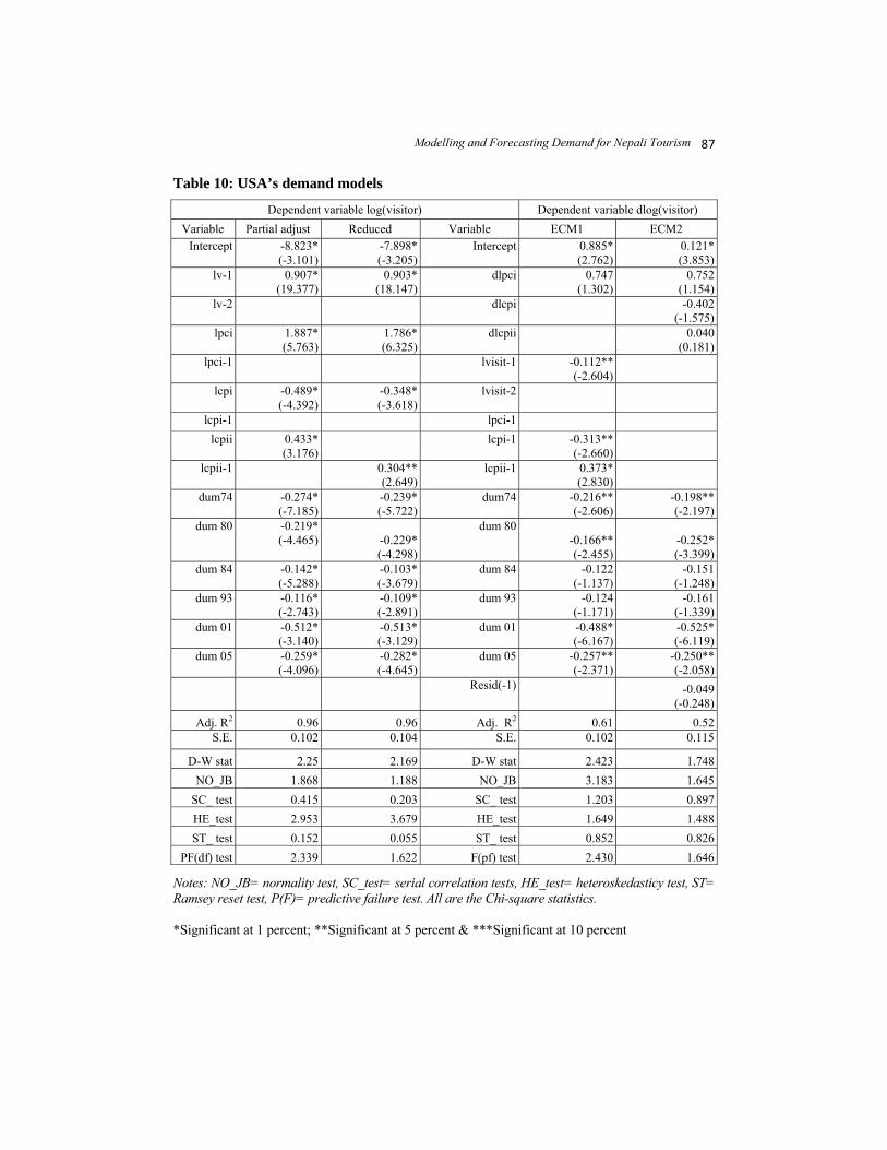
Modelling and Forecasting Demand for Nepali Tourism
87
Table 10: USA’s demand models
Dependent variable log(visitor) Dependent variable dlog(visitor) Variable Partial adjust Reduced Variable ECM1 ECM2
Intercept -8.823* (-3.101)
-7.898*(-3.205)
Intercept 0.885*(2.762)
0.121*(3.853)
lv-1 0.907* (19.377)
0.903*(18.147)
dlpci 0.747(1.302)
0.752(1.154)
lv-2
dlcpi -0.402(-1.575)
lpci 1.887* (5.763)
1.786*(6.325)
dlcpii 0.040(0.181)
lpci-1
lvisit-1 -0.112**(-2.604)
lcpi -0.489* (-4.392)
-0.348*(-3.618)
lvisit-2
lcpi-1 lpci-1lcpii 0.433*
(3.176) lcpi-1 -0.313**
(-2.660)lcpii-1
0.304**(2.649)
lcpii-1 0.373*(2.830)
dum74 -0.274* (-7.185)
-0.239*(-5.722)
dum74 -0.216**(-2.606)
-0.198**(-2.197)
dum 80 -0.219* (-4.465)
-0.229*(-4.298)
dum 80-0.166**(-2.455)
-0.252*(-3.399)
dum 84 -0.142* (-5.288)
-0.103*(-3.679)
dum 84 -0.122(-1.137)
-0.151(-1.248)
dum 93 -0.116* (-2.743)
-0.109*(-2.891)
dum 93 -0.124(-1.171)
-0.161(-1.339)
dum 01 -0.512* (-3.140)
-0.513*(-3.129)
dum 01 -0.488*(-6.167)
-0.525*(-6.119)
dum 05 -0.259* (-4.096)
-0.282*(-4.645)
dum 05 -0.257**(-2.371)
-0.250**(-2.058)
Resid(-1) -0.049(-0.248)
Adj. R2 0.96 0.96 Adj. R2 0.61 0.52S.E. 0.102 0.104 S.E. 0.102 0.115
D-W stat 2.25 2.169 D-W stat 2.423 1.748NO_JB 1.868 1.188 NO_JB 3.183 1.645
SC_ test 0.415 0.203 SC_ test 1.203 0.897HE_test 2.953 3.679 HE_test 1.649 1.488ST_ test 0.152 0.055 ST_ test 0.852 0.826
PF(df) test 2.339 1.622 F(pf) test 2.430 1.646
Notes: NO_JB= normality test, SC_test= serial correlation tests, HE_test= heteroskedasticy test, ST= Ramsey reset test, P(F)= predictive failure test. All are the Chi-square statistics. *Significant at 1 percent; **Significant at 5 percent & ***Significant at 10 percent
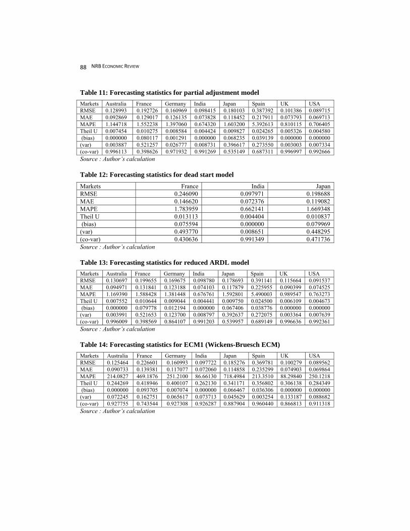
NRB ECONOMIC REVIEW
88
Table 11: Forecasting statistics for partial adjustment model Markets Australia France Germany India Japan Spain UK USA RMSE 0.128993 0.192726 0.160969 0.098415 0.180103 0.387392 0.101386 0.089715 MAE 0.092869 0.129017 0.126135 0.073828 0.118452 0.217911 0.073793 0.069713 MAPE 1.144718 1.552238 1.397060 0.674320 1.603200 5.392613 0.810115 0.706405 Theil U 0.007454 0.010275 0.008584 0.004424 0.009827 0.024265 0.005326 0.004580 (bias) 0.000000 0.080117 0.001291 0.000000 0.068235 0.039139 0.000000 0.000000 (var) 0.003887 0.521257 0.026777 0.008731 0.396617 0.273550 0.003003 0.007334(co-var) 0.996113 0.398626 0.971932 0.991269 0.535149 0.687311 0.996997 0.992666 Source : Author’s calculation Table 12: Forecasting statistics for dead start model
Markets France India Japan RMSE 0.246090 0.097971 0.198688MAE 0.146620 0.072376 0.119082 MAPE 1.783959 0.662141 1.669348 Theil U 0.013113 0.004404 0.010837 (bias) 0.075594 0.000000 0.079969 (var) 0.493770 0.008651 0.448295 (co-var) 0.430636 0.991349 0.471736Source : Author’s calculation Table 13: Forecasting statistics for reduced ARDL model Markets Australia France Germany India Japan Spain UK USA RMSE 0.130697 0.199655 0.169675 0.098780 0.178693 0.391141 0.115664 0.091537 MAE 0.094971 0.131841 0.123188 0.074103 0.117879 0.225955 0.090399 0.074525 MAPE 1.169390 1.588428 1.381448 0.676761 1.592801 5.490003 0.989547 0.763273 Theil U 0.007552 0.010644 0.009044 0.004441 0.009750 0.024500 0.006109 0.004673 (bias) 0.000000 0.079778 0.012194 0.000000 0.067406 0.038776 0.000000 0.000000 (var) 0.003991 0.521653 0.123700 0.008797 0.392637 0.272075 0.003364 0.007639 (co-var) 0.996009 0.398569 0.864107 0.991203 0.539957 0.689149 0.996636 0.992361 Source : Author’s calculation Table 14: Forecasting statistics for ECM1 (Wickens-Bruesch ECM) Markets Australia France Germany India Japan Spain UK USA RMSE 0.125464 0.226601 0.160993 0.097722 0.185276 0.369781 0.100279 0.089562 MAE 0.090733 0.139381 0.117077 0.072060 0.114858 0.235299 0.074903 0.069864 MAPE 214.0827 469.1876 251.2100 86.66130 718.4984 213.3510 88.29840 250.1218 Theil U 0.244269 0.418946 0.400107 0.262130 0.341171 0.356802 0.306138 0.284349 (bias) 0.000000 0.093705 0.007074 0.000000 0.066467 0.036306 0.000000 0.000000 (var) 0.072245 0.162751 0.065617 0.073713 0.045629 0.003254 0.133187 0.088682 (co-var) 0.927755 0.743544 0.927308 0.926287 0.887904 0.960440 0.866813 0.911318 Source : Author’s calculation

Modelling and Forecasting Demand for Nepali Tourism
89
Table 15: Forecast statistics for ECM2 (Johansen Maximum Likelihood ECM) Markets Australia France Germany India Japan Spain UK USA RMSE 0.167722 0.262373 0.167956 0.122109 0.117247 0.252196 0.119498 0.100439MAE 0.130389 0.189467 0.129272 0.089293 0.086708 0.197224 0.088681 0.079010 MAPE 580.3780 2.236396 296.2185 116.9032 1078.136 173.6339 116.6144 267.4820 Theil U 0.374097 0.014184 0.547063 0.336429 0.334530 0.399932 0.407904 0.322724 (bias) 0.000000 0.000000 0.000000 0.000000 0.000000 0.000000 0.000000 0.000000 (var) 0.170777 0.016329 0.379645 0.122130 0.126040 0.190945 0.246221 0.113014 (co-var) 0.829223 0.983671 0.620355 0.877870 0.873960 0.809055 0.753779 0.886986 Source : Author’s calculation Table 16: Forecasted growth rates for major markets for 2010 to 2020
Year Australia France Germany India Japan Spain UK USA Partial adjustment 9.77 11.08 16.24 3.75 9.63 17.94 12.49 11.63 Dead start 0.00 14.40 0.00 2.35 6.93 0.00 0.00 0.00 Reduced ARDL 10.30 11.27 12.78 3.86 9.50 17.47 13.85 9.75 ECM1 14.51 16.68 8.39 2.03 7.75 16.57 8.41 11.58 EcM2 17.02 12.68 8.69 27.24 8.85 9.25 8.40 13.55
2006-10(actual) 19.77 12.51 12.26 4.44 5.94 11.78 8.48 16.08 2005-2009 (actual) 12.65 5.13 5.77 0.85 0.26 5.12 8.78 10.86
2000-10(actual) 5.92 2.46 0.81 3.30 -3.79 8.95 1.26 2.13 2010-20(forecast) 2.56 2.39 2.81 3.55 1.99 1.23 1.83 2.28
Table 17: Forecasted number of the tourists from major markets for 2010 to 2020
Year Australia France Germany India Japan Spain UK USA Total
2010 15918 22838 19882 98847 22944 13562 36098 32875 519004
2011 17295 25028 24109 121284 23771 14107 36255 37917 611903
2012 17753 25636 24745 126247 24271 14283 36972 38749 620951
2013 18210 26244 25381 131211 24770 14459 37688 39581 629999
2014 18667 26852 26017 136174 25270 14635 38404 40414 639047
2015 19124 27460 26653 141137 25769 14810 39120 41246 648095
2016 19582 28068 27289 146100 26269 14986 39837 42078 657143
2017 20039 28676 27924 151063 26768 15162 40553 42910 666191
2018 20496 29283 28560 156026 27267 15338 41269 43742 675239
2019 20954 29891 29196 160990 27767 15514 41985 44574 684287
2020 21411 30499 29832 165953 28266 15689 42702 45406 693335 Source: Author’s calculation