University of Wollongong University of Wollongong

Research Online Research Online

University of Wollongong Thesis Collection 1954-2016 University of Wollongong Thesis Collections

2016

Modelling and control of electric vehicles with individually actuated in-Modelling and control of electric vehicles with individually actuated in-

wheel motors wheel motors

Sean Christifor McTrustry University of Wollongong

Follow this and additional works at: https://ro.uow.edu.au/theses

University of Wollongong University of Wollongong

Copyright Warning Copyright Warning

You may print or download ONE copy of this document for the purpose of your own research or study. The University

does not authorise you to copy, communicate or otherwise make available electronically to any other person any

copyright material contained on this site.

You are reminded of the following: This work is copyright. Apart from any use permitted under the Copyright Act

1968, no part of this work may be reproduced by any process, nor may any other exclusive right be exercised,

without the permission of the author. Copyright owners are entitled to take legal action against persons who infringe

their copyright. A reproduction of material that is protected by copyright may be a copyright infringement. A court

may impose penalties and award damages in relation to offences and infringements relating to copyright material.

Higher penalties may apply, and higher damages may be awarded, for offences and infringements involving the

conversion of material into digital or electronic form.

Unless otherwise indicated, the views expressed in this thesis are those of the author and do not necessarily Unless otherwise indicated, the views expressed in this thesis are those of the author and do not necessarily

represent the views of the University of Wollongong. represent the views of the University of Wollongong.

Recommended Citation Recommended Citation McTrustry, Sean Christifor, Modelling and control of electric vehicles with individually actuated in-wheel motors, Master of Philosophy thesis, School of Mechanical, Materials and Mechatronic Engineering, University of Wollongong, 2016. https://ro.uow.edu.au/theses/4737

Research Online is the open access institutional repository for the University of Wollongong. For further information contact the UOW Library: research-pubs@uow.edu.au

Modelling and Control of Electric Vehicles withIndividually Actuated In-Wheel Motors

Sean Christifor McTrustry

Supervisors:

Haiping Du, Phillip Commins

This thesis is presented as part of the requirements for the conferral of the degree:

Master of Philosophy (Mechatronic Engineering)

The University of Wollongong

School of Engineering and Information Sciences

March 2016

Declaration

I, Sean Christifor McTrustry, declare that this thesis submitted in partial ful-

filment of the requirements for the conferral of the degree Master of Philosophy

(Mechatronic Engineering), from the University of Wollongong, is wholly my own

work unless otherwise referenced or acknowledged. This document has not been

submitted for qualifications at any other academic institution.

Sean Christifor McTrustry

September 27, 2016

Abstract

Torque vectoring in electric ground vehicles (EGV) with individually

actuated in-wheel motors (IAIWM) presents the opportunity to imple-

ment a wide range of control strategies for controlling vehicle yaw rate

to improve vehicle stability and performance. The use of IAIWMs allows

for alternative vehicle layout configurations which previously would have

been unavailable to conventional internal combustion engine vehicles. The

use of higher level control architectures to distribute torque amongst the

two front wheel-drive, rear wheel-drive or four wheel-drive in-wheel mo-

tors of an electric ground vehicle has presented the opportunity to design

characteristics of electric ground vehicles through active control of power

trains. Previously in internal combustion engine vehicles, these character-

istics have been indirectly tuned via common chassis parameters. The use

of modern components such as in-wheel motors in electric ground vehicles

also provides additional benefits such as precise torque generation, fast mo-

tor response and the capability to produce forward and reverse torque as

well as regenerative braking to improve energy efficiency, and enabling the

estimation or measurement of useful feedback information. This feedback

information can be applied to direct yaw-moment control (DYC) strategies

which can be used to improve vehicle performance. The application of these

new vehicle configurations can allow for differential torque output to the

left and right hand side of vehicles, generating a yaw moment, and hence

directly affecting the yaw rate of the vehicle in a practice known as direct

yaw-moment control. In addition to the potential electric ground vehicles

possess for superior vehicle stability and performance, they are also a vi-

able solution for the environmental concerns pertaining to transport needs

and meeting lower emissions targets. In this thesis the process of convert-

ing an internal combustion engine vehicle to a fully electric vehicle with

IAIWM will be presented. The first aim of this thesis is to conduct a lit-

erature review in which control strategies available for allocating torque to

i

individually actuated in-wheel motors on an electric ground vehicle are in-

vestigated, with the objectives of improving vehicle dynamics performance

through control of yaw rate response. Secondly, this thesis will present the

development of a simulation framework which models vehicle behaviour

and addresses the major performance indicators relevant to evaluating ve-

hicle dynamics performance with regards to torque vectoring(TV)/DYC

strategies. Next, this thesis aims to show the effects of a traction control

strategy, developed for active differentials, when adapted and extended for

use as a direct yaw-moment control strategy on an electric ground vehicle

with individually actuated in-wheel motors. This torque vectoring control

strategy’s effect on a vehicle’s dynamic performance will be validated and

analysed through use of simulations, using the platform developed as part

of the work involved in this thesis. The simulation platform presented in

this thesis is also intended for use as tool for investigation on future projects

pertaining to the experimental electric vehicle. The next objective of this

thesis is to establish the measurement and estimation techniques available

and how they could be implemented through suitable hardware to measure

and record the relevant performance indicators of vehicle dynamics in re-

lation to a DYC strategy. Finally, this thesis aims to prove the accuracy of

the simulation platform developed using experimental data acquired from

sensors implemented on the experimental vehicle. The simulation platform

is validated experimentally as an accurate representation of the experi-

mental system and its performance in terms of realistic vehicle dynamics.

Experimental data is used to recreate real-life driving manoeuvres in the

simulation platform, and verify its performance by comparing results.

ii

Acknowledgements

• Phil Commins

• Haiping Du

• Uow & Innovation Campus Technical Staff

iii

Contents

1 Introduction 1

2 Literature Review 4

2.1 Background and Context . . . . . . . . . . . . . . . . . . . . . . . 4

2.1.1 Torque Vectoring and DYC Background . . . . . . . . . . 5

2.1.2 Important Performance Indicators . . . . . . . . . . . . . . 11

2.2 Estimation Based Techniques for Vehicle Control . . . . . . . . . 16

2.3 Longitudinal Wheel Slip Based Techniques for Yaw Rate Control . 18

2.4 Vehicle Side-slip Angle DYC Strategies . . . . . . . . . . . . . . . 21

2.5 Yaw Rate DYC Strategies . . . . . . . . . . . . . . . . . . . . . . 23

2.6 Integrated Control Systems . . . . . . . . . . . . . . . . . . . . . 26

3 Vehicle Dynamics and Modelling 30

3.1 Experimental Vehicle Properties . . . . . . . . . . . . . . . . . . . 30

3.2 Tyre and Wheel Model . . . . . . . . . . . . . . . . . . . . . . . . 32

3.3 Vehicle Model and Equations of Motion . . . . . . . . . . . . . . . 33

4 Research Design and Methodology 36

4.1 Electric Vehicle Conversion . . . . . . . . . . . . . . . . . . . . . . 36

4.2 Modelling of the System . . . . . . . . . . . . . . . . . . . . . . . 38

4.2.1 SimDriveLine . . . . . . . . . . . . . . . . . . . . . . . . . 39

4.2.2 Simscape/SimMechanics . . . . . . . . . . . . . . . . . . . 42

4.3 Data Acquisition and Estimation Techniques . . . . . . . . . . . . 49

4.3.1 VBOX . . . . . . . . . . . . . . . . . . . . . . . . . . . . . 49

4.3.2 Android/iOS Accelerometer and Gyroscopic Sensor Sup-

port from MATLAB . . . . . . . . . . . . . . . . . . . . . 53

iv

4.3.3 Motor Controller . . . . . . . . . . . . . . . . . . . . . . . 55

4.3.4 Encoder . . . . . . . . . . . . . . . . . . . . . . . . . . . . 55

4.3.5 Controller Area Network (CAN) Bus . . . . . . . . . . . . 56

4.4 Summary . . . . . . . . . . . . . . . . . . . . . . . . . . . . . . . 57

5 Controller Definitions and Simulated Results 58

5.1 Longitudinal Wheel Slip Regulation DYC for Front-Wheel Drive

Electric Vehicle Controller Definition . . . . . . . . . . . . . . . . 58

5.1.1 Simulated Results . . . . . . . . . . . . . . . . . . . . . . . 62

5.2 Longitudinal Wheel Slip Regulation for Electric Vehicle with Four

IAIWM Controller Definition . . . . . . . . . . . . . . . . . . . . 63

5.2.1 Simulated Results . . . . . . . . . . . . . . . . . . . . . . . 67

5.3 Longitudinal Wheel Slip Regulation with PI Controller for Electric

Vehicle with Four IAIWM Controller Definition . . . . . . . . . . 68

5.3.1 Simulated Results . . . . . . . . . . . . . . . . . . . . . . . 68

5.3.2 Summary . . . . . . . . . . . . . . . . . . . . . . . . . . . 70

5.4 Longitudinal Performance Control . . . . . . . . . . . . . . . . . . 73

5.4.1 Simulated Results . . . . . . . . . . . . . . . . . . . . . . . 75

5.5 Summary of Simulated Results . . . . . . . . . . . . . . . . . . . 77

6 Experimentally Acquired Results and Validation 80

6.1 Validation of Simulation Platform . . . . . . . . . . . . . . . . . . 80

6.1.1 Experimentally Verified Results . . . . . . . . . . . . . . . 84

7 Future Work and Conclusions 95

7.1 Future Work and Applications . . . . . . . . . . . . . . . . . . . . 95

7.2 Conclusions . . . . . . . . . . . . . . . . . . . . . . . . . . . . . . 97

v

List of Tables

1 Vehicle Properties . . . . . . . . . . . . . . . . . . . . . . . . . . . 30

vi

List of Figures

1 Controller layout for design proposed by Doniselli et. al. [1]. . . . 24

2 Diagram detailing the layout of a typical Ackerman steering mech-

anism. . . . . . . . . . . . . . . . . . . . . . . . . . . . . . . . . . 31

3 Motor fitting to vehicle assembly modelled in CREO Parametric. . 38

4 Top level of SimDriveLine model of an electric ground vehicle with

four in-wheel motors. . . . . . . . . . . . . . . . . . . . . . . . . . 40

5 Base level of SimDriveLine model of an electric vehicle with four

in-wheel motors. . . . . . . . . . . . . . . . . . . . . . . . . . . . . 41

6 Comparison of the modelled vehicle in simulation and the experi-

mental vehicle. . . . . . . . . . . . . . . . . . . . . . . . . . . . . 42

7 Simulink model of the electric vehicle with sensing and torque

distribution control. . . . . . . . . . . . . . . . . . . . . . . . . . . 44

8 Flow diagram detailing the layout of the Simulink model of the

electric vehicle. . . . . . . . . . . . . . . . . . . . . . . . . . . . . 45

9 Low fidelity implementation of Ackerman steering mechanism for

performing a J-turn manoeuvre. . . . . . . . . . . . . . . . . . . . 47

10 Tikz diagrams of vehicle components. . . . . . . . . . . . . . . . . 48

11 Tikz diagram of the layout of the vehicle’s front suspension system. 49

12 Tikz diagram of the layout of the vehicle’s rear suspension system. 50

13 Modified mask for tyre models to extend vehicle testing to acco-

modate split and instantaneous split slippery surface conditions. 51

14 VBOX20SL Dual Antenna Module. Image courtesy of [2]. . . . . 52

15 Standard layout of measurable axes on a mobile device. Image

courtesy of [3]. . . . . . . . . . . . . . . . . . . . . . . . . . . . . . 53

16 Graphical user interface for Android/iOs Sensor Support on MAT-

LAB Mobile. Image courtesy of [3]. . . . . . . . . . . . . . . . . . 54

vii

17 Rotary encoder employed for measuring steering wheel angle in

the experimental vehicle. . . . . . . . . . . . . . . . . . . . . . . . 56

18 Simulink diagram of subsystem for generating a reference torque

signal to simulate the driver’s input from the acceleration pedal. . 61

19 Simulink model of Doniselli et. al. control law adapted for vehicles

with in-wheel motors. . . . . . . . . . . . . . . . . . . . . . . . . . 62

20 Yaw rate response of uncontrolled front-wheel-drive EV performing

J-turn manoeuvre. . . . . . . . . . . . . . . . . . . . . . . . . . . 62

21 Yaw rate response of longitudinal wheel slip regulation algorithm

adapted for front-wheel-drive EV with in-wheel motors performing

a J-turn manoeuvre. . . . . . . . . . . . . . . . . . . . . . . . . . 63

22 Uncontrolled longitudinal wheel-slip for front-wheel-drive EV (sim-

ulated). . . . . . . . . . . . . . . . . . . . . . . . . . . . . . . . . 64

23 Controlled longitudinal wheel-slip for front-wheel-drive EV (simu-

lated). . . . . . . . . . . . . . . . . . . . . . . . . . . . . . . . . . 65

24 Simulink model of longitudinal slip ratio (Doniselli et. al.) control

law extended to vehicles with four in-wheel motors. . . . . . . . . 67

25 Simulated yaw rate response of an uncontrolled vehicle performing

a J-turn manoeuvre. . . . . . . . . . . . . . . . . . . . . . . . . . 68

26 Simulated yaw rate response of vehicle with four IAIWM and lon-

gitudinal slip ratio control performing a J-turn manoeuvre . . . . 69

27 Simulink model of longitudinal slip ratio control law including pro-

portional and integral gain terms. . . . . . . . . . . . . . . . . . . 70

28 Simulated yaw rate response of system performing a J-turn ma-

noeuvre with proportional and integreal gain terms included. . . . 71

29 Longitudinal wheel slip of each tyre for uncontrolled EV with four

IAIWM performing J-turn manoeuvre. . . . . . . . . . . . . . . . 71

viii

30 Longitudinal wheel slip of each tyre for controlled EV with four

IAIWM performing J-turn manoeuvre. . . . . . . . . . . . . . . . 72

31 Simulated yaw rate response of uncontrolled system performing a

line change manoeuvre. . . . . . . . . . . . . . . . . . . . . . . . . 72

32 Simulated yaw rate response of system performing a line change

manoeuvre with proportional and integreal gain terms included. . 73

33 Application of control law expressed as a Simulink model. . . . . . 74

34 Comparison of uncontrolled vehicle velocity under split-slippery

surface conditions and controlled vehicle velocity under split-slippery

surface conditions. . . . . . . . . . . . . . . . . . . . . . . . . . . 76

35 Comparison of the effect on vehicle yaw rate on split slippery sur-

face conditions for straight line driving for uncontrolled and con-

trolled systems. . . . . . . . . . . . . . . . . . . . . . . . . . . . 77

36 Simulated yaw rate response to J-turn manoeuvre for an uncon-

trolled, front-wheel drive vehicle. . . . . . . . . . . . . . . . . . . 78

37 Simulated yaw rate response to J-turn manoeuvre for an uncon-

trolled vehicle with four IAIWM. . . . . . . . . . . . . . . . . . . 78

38 Simulated yaw rate response to J-turn manoeuvre for a vehicle

with four IAIWM and longitudinal slip ratio controller implemented. 79

39 Simulated system response of displacement over time to even torque

distribution. . . . . . . . . . . . . . . . . . . . . . . . . . . . . . . 81

40 Simulated system response of displacement over time to a biased

torque distribution. . . . . . . . . . . . . . . . . . . . . . . . . . . 81

41 Simulated and theoretically calculated forward velocity of the sim-

ulated vehicle model. . . . . . . . . . . . . . . . . . . . . . . . . . 82

42 Comparison of simulated wheel slip acquired with unaltered and

quantized data for wheel angular velocity. . . . . . . . . . . . . . 83

ix

43 Steering wheel angle measured from encoder on experimental vehi-

cle steering shaft and replicated signal built on Simulink for input

to simulated vehicle. . . . . . . . . . . . . . . . . . . . . . . . . . 85

44 Torque output measured from experimental vehicle and replicated

signal built on Simulink for input to simulated vehicle. . . . . . . 86

45 Comparison of simulated and measured yaw rate response of the

vehicle whilst performing the same maneouver. . . . . . . . . . . . 86

46 Comparison of absolute vehicle speed for the experimental and

simulated vehicles. . . . . . . . . . . . . . . . . . . . . . . . . . . 88

47 Comparison of simulated and experimentally acquired values for

longitudinal wheel slip of the front-left tyre. . . . . . . . . . . . . 90

48 Experimentally measured sideslip measured from the vehicle centre

of gravity. . . . . . . . . . . . . . . . . . . . . . . . . . . . . . . . 92

49 Simulated vehicle sideslip front left and front right tyres. . . . . . 93

50 Desired and actual yaw rate of line change manoeuvre. . . . . . . 94

x

List of Abbreviations and Symbols

CAD Computer Aided Design

CAN Control Area Network

DYC Direct Yaw-moment Control

EGV Electric Ground Vehicle

EV Electric Vehicle

GPS Global Positioning System

GUI Graphical User Interface

IAIWM Independently Actuated In-Wheel Motors

OAEGV Over-Actuated Electric Ground Vehicle

PI Proportional-Integral

PID Proportional-Integral-Derivative

PMSM Permanent Magnet Synchronous Machine

TV Torque Vectoring

xi

1 Introduction

The motivation for this project lies in the increasing demand for low environ-

mental impact vehicles with adequate performance characteristics [4]. Internal

combustion engine vehicles are a major contributor to greenhouse gas emissions,

airborne pollution, carbon monoxide and air toxins [4]. With a significantly less

profound impact on the environment than internal combustion engine vehicles [5],

electric ground vehicles are identified as a potential technology for meeting the

demand for low environmental impact vehicle [6]. Research and development

on electric ground vehicles has been increasing and as a result, improvements in

energy usage and control technology has been achieved [7].

The majority of passenger vehicles available on the market today make use of a

single engine drivetrain, which distributes power to two or four wheels through

a gearbox and differentials [8]. Electric ground vehicles may use different con-

figurations, which can have a profound effect on the vehicle’s performance and

efficiency characteristics. One configuration of electric ground vehicles which has

shown improved results in vehicle performance characteristics is the use of four

individually actuated in-wheel motors [9]. This setup features either a direct

drive or reduction drivetrain on each wheel. These in-wheel motors allow for

improved vehicle control, as they are part of the vehicles unsprung mass, and

are used to actively design performance characteristics, as opposed to indirectly

tuning them via the common chassis system [8]. Use of electric motors at each

wheel also allows for improved accuracy in measuring vehicle characteristics, as

each motor can be used as a measuring device for individual wheel speed. The

major contributions of in-wheel motor technology to electric vehicle perfomance

can be categorised into precise and fast torque generation, efficient feedback in-

formation on motor torque and speed output and ease of producing torque in

both forward and reverse directions [10]. These characteristics allow for more

accurate measurements and estimations to be made regarding vehicle dynamics

1

behaviour and road surface conditions to allow the vehicle to adjust its torque

allocation to improve performance.

The benefits of in-wheel motor technology as outlined above can be applied to the

design of a control architecture with the purpose of distributing torque amongst

the driving wheels of the electric vehicle. The measured and estimated data which

can be acquired from this vehicle layout configuration allows for the design of a

a more effective torque vectoring control strategy. The practice of using differen-

tial torque outputs to generate a yaw moment for directly altering the vehicle’s

motion about the vertical axis and improving vehicle stability is oftern referred

to as direct yaw-moment control (DYC) [11]. An effective means of improving a

vehicle’s dynamic performance is through the measurement and control of vehicle

yaw rate. This strategy invovles a controller which is designed with the objective

of bringing the vehicle’s measured yaw rate into conformity with the optimal yaw

rate by calculating and producing a corrective yaw moment via torque vectoring

control [12]. Use of in-wheel motor technology in conjunction with direct yaw-

moment control is a growing area of research in both academia and commercial

research and development which has produced significant improvements in the

handling and stability of passenger vehicles [13].

The first aim of this project is to convert an internal combustion engine vehicle,

into an electric ground vehicle with individually actuated in-wheel motors. The

objective being to function as a useful platform for future projects performing

research into optimal energy efficiency and vehicle performance via higher level

control. Secondly, this project aims to create a simulation model to function

as an accurate representation of the experimental vehicle, serving as a robust

and versatile platform for inspecting higher level vehicle control functions and

their effect on vehicle performance. This project also aims to experimentally val-

idate this model by measuring and comparing the key performance indicators of

the simulation with experimentally obtained results on the experimental vehicle.

2

Thirdly, this project aims to establish a feasible strategy for the acquistion of

useful data in real time which can be implemented into vehicle control, such as

a torque vectoring control strategy. Finally, this project performs research into

the current state of the art in torque vectoring control applications, with the

aim to explore the practicality of developing a suitable torque vectoring control

strategy, based on direct yaw-moment control (DYC) to improve vehicle yaw rate

response and the handling and stability of the vehicle. The effectiveness of this

strategy will be proved through simulations and its feasibility evaluated based on

the resources required and process involved in implementing this strategy on a

real system. The findings of this research, along with the results of simulations

and experimental work performed will be detailed in this thesis, to establish a

strategy and validate its feasibility in achieving this objective.

3

2 Literature Review

In recent years, in response to demand for commercial vehicles with reduced en-

vironmental impact [5], there has been an increased devotion of time and effort

into the research and development of new configurations, technological devel-

opments and control strategies for electric ground vehicles [14]. The concept

of using individually actuated in-wheel motors in electric ground vehicles has

been explored by a number of institutions [13] the world over in pursuit of im-

proving vehicle dynamics performance through torque vectoring and yaw rate

control. In this chapter a review of the various methods of direct yaw-moment

control via torque vectoring for electric vehicles is presented. Torque vectoring

is based on the strategic distribution of torque to the driving wheels of a vehi-

cle to improve the vehicle’s dynamic performance. Methods of torque vectoring

and direct yaw-moment control in electric vehicles varies based on the configura-

tion of vehicle hardware and the control variables in use . The vehicle hardware

configuration may consist of active differentials, drivetrains with individual mo-

tors, or in-wheel motors to deliver the controlled torque to the vehicle’s driving

wheels. Various torque vectoring strategies can be categorised depending on the

control variable each utilises. This chapter will provide some background con-

text on direct yaw-moment control via torque vectoring, review the important

performance indicators relevant to applying an effective control strategy and re-

view direct yaw-moment control strategies based on feedback of yaw rate, vehicle

side-slip angle, and longitudinal slip ratio.

2.1 Background and Context

This section will provide background information and context relevant to the

project. Concepts such as applications of torque vectoring and introducing feed-

back loops to yaw rate control helped to shape the current state of the art for

DYC. Some examples which have been documented in literature will be discussed

4

in this section, along with important performance indicators relevant to the de-

sign of a DYC strategy.

2.1.1 Torque Vectoring and DYC Background

Torque vectoring refers to the distribution of torque from the engine to the wheels

of a ground vehicle. Conventionally, torque vectoring in an internal combustion

engine vehicle uses a differential to distribute torque from the engine to the axles

of the vehicle. The research and application of torque vectoring control as a tech-

nique for the improvement of a vehicle’s dynamic performance is a growing area of

interest in research and development in both industry and academia [15]. Active

torque distribution is a relatively new concept, as the majority of literature on the

subject has been published within the last ten years, but has progressed in both

complexity and quality of results produced in recent years with the development

of new technology such as hub motors (in-wheel motors).

Previously, applications of in-wheel motor technology were primarily for the use

of vehicles such as bicycles and electric scooters [16] but this technology has seen

significant development in recent years and as such their usefulness in passen-

ger vehicle technology has been utilised [13]. The application of active torque

vectoring control evolved from using a differential to distribute torque, to the

use of active drive devices such as electronic limited slip differentials, on-demand

centre couplings [17], front or rear electric axels with distributed torque [18] to

the current state of the art which makes use of in-wheel motors in conjunction

with a control architecture to distribute torque to each wheel. The application

of in-wheel motors as a means of active torque distribution allows for the hub

motors to be part of the vehicle’s unsprung mass, and allows for the active con-

trol of the distribution of torque, as opposed to indirectly tuning common chassis

parameters to rely on the distribution of torque [8]. Utilising torque vectoring

methods to deliver a torque differential across the left and right hand wheels of

5

a vehicle can be used to generate a yaw moment, which is used to directly alter

the yaw rate of the vehicle. This practise is known as direct yaw-moment control

(DYC) [11].

Prior to the use of in-wheel motors, active drive components have been utilised

in electric vehicles to apply torque vectoring control techniques which produced

improvements to vehicle handling and stability [18,19] due to the advantage pro-

vided by active differentials as they do not require brake or throttle intervention

when compared to previously implemented yaw rate control strategies [20]. Work

performed by Hancock et. al. [21] and Ikushima and Sawase [22] both developed

direct yaw-moment control strategies based on the use of actively controlled me-

chanical differentials. Osborn et. al. performed studies into independent wheel

actuation to explore its effectiveness in improving vehicle stability during criti-

cal steering manoeuvres whilst the vehicle is under acceleration. A straegy was

adopted using a proportional-integral controller to apply yaw feedback to dis-

tribute torque to the front-rear wheels, and lateral acceleration feedback was used

to adjust the torque distribution from the left and right hand driving wheels of

the vehicle. A similar approach was adopted by De Novellis et. al. comparing

feedback control techniques for a front-wheel-drive electric vehicle, with two in-

dividual power trains, one for each of the front wheels [9]. Yaw motion control

through use of active differentials was also explored by Hancock et. al. [20] in

which an active rear wheel drive system was shown to significantly modify a ve-

hicle’s dynamics performance through active control of lateral torque distribution

on the vehicle’s rear axel. Osborn et. al. evaluated system performance by com-

paring a front-wheel-drive, and rear-wheel-drive both with a single open differen-

tial, and an all-wheel-drive model with three open differentials to the model with

fully independent torque distribution, and front-rear torque distribution control

implemented. These configurations were tested under a standard manoeuvre;

response to steering input of 5 degrees. The results showed that of all the mod-

els evaluated, the model with independent torque control maintained the closest

6

conformity to the desired path of the vehicle, without affecting the acceleration

of the vehicle. The limitations of this work performed include simplifications that

were made to the vehicle model. The model is based on Newtonian equations

and the Pacejka Magic Tyre Formula, however the model ignores heave, roll and

pitch motion, has no suspension included, assumes the exact torque requested

can be applied instantaneously to each wheel and assumes steering angles of each

wheel are identical. Results were obtained using a seven degree of freedom vehicle

model developed in Simulink using the Pacejka Magic Tyre Formula [23].

Another typical method of DYC is a control technique based on the Ackerman

steering geometry. This technique involves calculating the desired angular veloc-

ity of each of the driving wheels in a front-wheel driven vehicle with an Ackerman

steering mechanism. The relationship between wheel angular velocity and the

Ackerman steering mechanism can be expressed as follows:

ωL =vLR

=vrR

(1− dr tan δ

2l) (1)

ωR =vRR

=vrR

(1− dr tan δ

2l) (2)

Where R is the radius of the tyre, δ is the average of the front wheel’s steering an-

gles, vLand vR are the velocity of the rear left and rear right wheels respectively,

vr represents the velocity of the rear axle at the centre and ωL and ωR represent

the angular velocities of the front left and front right wheels respectively. Using

this relationship, the angular velocity of the two front driving wheels are con-

trolled based on their optimal values as set out by equations (1) and (2) when

cornering [12]. The effectiveness of this method has been confirmed through

simulated and experimental data for vehicles travelling at low speeds [24, 25].

The system is used to generate a yaw moment when cornering by reducing the

angular velocity of the inner-wheel, and increasing the angular velocity of the

outer-wheel [26]. However, it is important to note that this technique is only ef-

fective at low speeds, when vehicle side-slip does not occur. The effect of vehicle

7

side-slip which occurs during cornering at higher speeds creates lateral motion

which affects the size of the turning radius of the vehicle, therefore making the

equations which govern this control strategy innacurate. This technique does not

utilise feedback control, but it was a method which served to provide foundations

for research into more advanced direct yaw-moment control techniques.

De Novellis et. al. explore the use of feedback control for vehicle yaw rate and

perform an objective comparison of yaw rate control torque alloaction techniques

and compare four different approaches. A PID control with feedforward contri-

bution, adaptive PID control with feedforward contribution, second order sliding

mode control based on the sub-optimal algorithm and second order sliding mode

control based on the twisting algorithm are compared with a baseline (uncon-

trolled) vehicle [9]. Generally vehicle side-slip angle can be maintained within

the vehicle’s stability limits through implementation of a yaw rate controller,

provided that friction coefficient of the the road surface and tyre are accurately

measured/estimated, given a correct reference yaw rate is generated. Estimation

is assumed to be implemented accurately, so as to focus on the comparison of

the yaw rate controllers. Performance of the controller is assessed through a per-

formance weighted function, which has been weighted to prioritise achievement

of the reference yaw rate with respect to the minimisation of the control action

required. Results are attained using a CarMaker vehicle model in which the

front axel has two independently controlled drivetrains. The robustness of each

controller is assessed by testing with two tyre topologies and by varying vehicle

weight and friction coefficient whilst undertaking ramp steer, step steer, tip-in

during cornering and frequency response (sinusoidal steering input) manoeuvres.

The results of these analyses indicate that the PID algorithms produce good

tracking performance and response to variations indicate a robust control sys-

tem. Additionally, the use of the sub-optimal sliding mode has been shown to

further enhance tracking performance. The relevance of this literature served

to establish the potential of using feedback loops as a part of vehicle dynamic

8

control for active drive train technology.

The progression of hub motor technology along with the literature previously

produced on active drive techniques focussing on controlling vehicle yaw rate has

enabled the progression of research in this field and allowed for improvements in

results. The use of electric motors and in-wheel motors’ enable sensing capabil-

ities which provide information to the control system that is implemented into

feedback loops, and offers a fast response to input of torque or speed demands [7].

Direct yaw-moment control is a prominent subject in literature concerned with

improving the stability and peformance of electric vehicles with individually ac-

tuated in-wheel motors. Research has revealed many apporaches that have been

applied to this technique with variations in design of hardware, logic and con-

trollers [11, 13,18,27–30].

Torque vectoring control of individually actuated in-wheel motors has also been

shown to enhance the operational energy usage and efficiency of electric vehi-

cles [31] and maximising their travel range [32]. Wang et. al. [32] obtained ex-

perimental results through use of an electric vehicle equipped with four in-wheel

motors and tested on a dynamometer. The efficiency of the battery to motors,

and efficiency of battery to ground is studied by Wang et. al. [32]. The strategy

adopted essentially involves minimising the use of battery power during driving

mode to reduce power consumption, and maximising battery power during brak-

ing to regenerate maximum power from the wheels at a given braking torque.

Qian et. al. [31] explored an optimal driving torque distribution strategy to min-

imise the use of electrical energy, and validated results through simulation using

Matlab, comparing the four indepdent-wheel drive vehicle with a single-engine

driven electric vehicle, and successfully showed that the use of four independently

actuated motors are more efficient than using one electric motor. Energy savings

were measured from the simulation as high as 27.4% when comparing the opti-

mal torque distribution strategy to a single-engine electric vehicle, however the

9

model explored accounted only for the vehicle under acceleration, and did not

account for any improvements in optimising regenerative braking. The research

performed by Wang et. al. also indiciated there was potential to increase an elec-

tric vehicle’s energy usage through torque distribution strategies not only whilst

under vehicle acceleration but also during regenerative braking.

An alternative to using feedback control of electric vehicles with individually ac-

tuated in-wheel motors to improve vehicle dynamics performance is model based

control. Model based control utilises a mathematical model to predict the torque

demand required to achieve the desired vehicle yaw rate [33]. This approach

calculates a desired yaw rate as a result of steering angle, which is used as input

to the system, and calculates the torque demand to each wheel to achieve the

desired yaw rate to be used as system outputs. This is sometimes referred to

as an inverse model approach. The benefits of applying model based approach

as opposed to feedback approach include a more rapid response, reductions in

time lag and undesired oscillations in response, provided that the model is an

accurate approximation of the inverse of the system. Model based control has

also been applied to improving the range of electric vehicles through optimisation

of the distribution of driving and braking forces between the wheels [34]. The

implications of this research are relevant as the range of electric vehicles when

compared to internal combustion engine vehicles for the use of passenger vehicles

is a limiting factor in their practicality. When applying a model based control

strategy for optimisation of distribution of torque between front and rear wheels

during acceleration and braking for straight line driving, an increase in range

of 2.8 km was recorded. A limitation of this study however is that the model

described in this source assumes that the left-right torque signals are even for

straight line driving and accounts for only straight line driving. There is no solu-

tion proposed for utilising model based control for optimising torque distribution

during driving which requires steering manoeuvres. An absence in literature is

evident on model based systems for improving vehicle dynamics performance,

10

which provides a possible avenue of research to pursue.

2.1.2 Important Performance Indicators

In terms of evaluating an electric ground vehicle’s performance and stability,

there are certain key performance indicators and performance objectives which

are commonly measured and used in controller design [7,8,33]. Depending on the

setup of the vehicle, and the control variables required for the controller, these

values can either be measured, calculated using measured variables or acquired

through use of estimation techniques. There are also other quantities relevant to

the vehicle and its environment which can be useful in evaluating and improving

the performance of an electric vehicle when designing and implementing a DYC

strategy. This section of the paper will detail the relevance of longitudinal wheel-

slip ratio, side-slip angle and yaw rate and how they are related to a vehicle’s

dynamic performance.

Longitudinal Wheel Slip Longitudinal wheel slip represents the relationship

between the tyre-road surface, forward velocity of the tyre, and its angular rota-

tional speed. This relationship is not categorised by a single formula or definition,

there are a number of accepted formulas used to define the longitudinal wheel

slip of a vehicle [35]. One commonly accepted definition of this relationship is

shown by:

κ = −Vx − reΩVx

(3)

Where κ represents longitudinal wheel slip, Vx is the longitudinal component of

the total velocity vector of the wheel centre, re is the effective rolling radius of

the tyre, and Ω is the angular speed of revolution of the tyre [23]. Alternatively,

11

another representation of this relationship is expressed as [36]:

λ =

(ΩRc

V− 1

)∗ 100% (4)

Where in this definition, λ is the slip ratio (expressed as a percentage), Ω is the

wheel’s angular velocity, Rc is the effective radius of the tyre and V is the vehicle

velocity. Both definitions are generally accepted and producde similar results for

evaluating the slip ratio of a given tyre on a vehicle.

Longitudinal wheel slip is an important relationship, as the occurence of signifi-

cant wheel slip is representative of a loss of traction between the tyre and road

surface, which can affect vehicle stability as well as the lateral and longitudinal

dynamic performance of the vehicle. The tyres which are experiencing wheel slip

may not be delivering sufficient torque to the road surface resulting in a loss

of longitudinal acceleration. Similarly, tyres experiencing significant wheel slip

and delivering reduced torque may alter the mangitude and direction of the to-

tal yaw moment generated by the vehicle affecting cornering behaviour, lateral

performance and overall control of the vehicle [37].

Vehicle Side-slip Angle Vehicle side-slip angle is often used as a performance

indicator when measuring a torque vectoring strategy’s effect on the lateral per-

formance of a vehicle, and is often used as the main control variable on which

a controller is based on. If the magnitude of a vehicle’s side-slip angle increases

to a large value, the vehicle loses capability to produce a yaw moment, which is

resultant in the vehicle’s reduced stability. This occurs due to a decrease corner-

ing stiffness in the tyres and yaw moment generated by lateral tyre forces [38].

Conversely, when the magnitude of vehicle side-slip angle is small, a consistency

between vehicle heading and the vehicle’s forward velocity vector is inherent,

which provides the driver with improved control of the vehicle during cornering

manoeuvres [39]. Given these findings, common practice in DYC strategies which

12

employ side-slip angle as a control variable aim to maintain a side-slip angle of

zero, or maintain vehicle side-slip angle within a stable region, to maintain vehi-

cle stability and controllability. Lateral wheel slip is defined as the ratio of the

lateral velocity and the forward velocity of the wheel. This value corresponds to

the negative tangent of the slip angle [23]; hence, the vehicle side-slip angle (α)

is defined in (2) as:

tanα = −VyVx

(5)

where Vx is the longitudinal component of the total velocity vector of the wheel

and Vy is the lateral component of the total velocity vector. Vehicle side-slip angle

is commonly measured when evaluating the dynamic performance of a vehicle

as the torque distribution strategy in place often has an objective to maintain

the side slip as low as possible to ensure lateral stability of the vehicle [9]. The

relationship between vehicle velocity and vehicle side-slip angle has been shown to

have an effect on vehicle turning behaviour, depending on the steering behaviour

of the vehicle i.e. if the vehicle is undergoing oversteer, understeer or neutral

steer behaviour. For understeer, side-slip angle reaches a maximum value at

larger velocities, for oversteer side-slip angle approaches negative infinity, and for

neutral steer, vehicle velocity does not affect the magnitude of side-slip angle [40].

A general expression for obtaining the reference value for desired vehicle side-slip,

in cases where controllers aim to track a desired vehicle side-slip response can be

expressed as follows:

β =

(lr − mlfv

2x

lCαr

)δ

l (1 +Kv2x)(6)

Where β is side-slip angle, lr is distance from centre of gravity to rear axel, lf is

distance from centre of gravity to front axel, vx is vehicle longitudinal velocity,

Cαr is total cornering stiffness of the rear tyres, l is the wheel base and K is the

13

stability factor (which will be explained in the following section).

Yaw Rate Yaw rate is another important performance indicator which reflects

the effectiveness of the torque distribution strategy in place. Yaw rate control is

one of the main aspects of vehicle stability control in modern passenger cars [9]

and is commonly used as the main control variable in vehicles with direct yaw-

moment control. The objective of the controller is to distribute torque to generate

a corrective yaw moment to bring the vehicle’s measured yaw rate into conformity

with the desired yaw rate [27]. Yaw rate control may be based on a number of

properties, including the estimated friction coefficient of the road surface, the

steering wheel angle and the vehicle velocity. A common strategy for yaw rate

control is designing a controller which inspects the error between the measured

yaw rate and reference (desired) yaw rate generated by the control system using

the steady state yaw response derived from the two degree of freedom vehicle

model [41]. A common form for this expression is shown below in equation (7):

rd =Vx

l(1 +KV 2x )δ (7)

Equation (7) is a function of the driver’s steering wheel angle input and vehicle

speed, where Vx is the vehicle longitudinal velocity, l is the length between front

and rear axles, δ is the steering wheel angle and K is the stability factor [27]

derived from the vehicle’s properties of mass, wheel base and cornering stiffness

of front and rear axles. The stability factor is used to adjust the optimal turning

radius to neutral steering behavior, understeer or oversteer [12]. The stability

factor K is defined as:

K =m

l2

(lrCαf− lfCαr

)(8)

Wherem represents vehicle mass, lf and lr represent the distance from the vehicle

centre of gravity to the front and rear axels respectively and Cαf and Cαr represent

the total cornering stiffness of the front and rear tyres respectively. Vehicle

14

turning radius is defined by the relationship:

R =v

r(9)

Where R is the vehicle turn radius, v is the resultant velocity of the vehicle centre

of mass (in cases where vy is very small, this value can be approximated simply

to vx) and r is the vehicle yaw rate. Substituting this relationship into equation

(7) results in the following relationship:

R =l (1 +KV 2

x )

δ(10)

Equation 10 demonstrates the relationship between vehicle velocity and turning

radius, and how the sign of the stability factor is a representation of steering

behaviour. Equation (10) shows that with a postive stability factor, turning ra-

dius increases with increasing vehicle speed, representing understeer behaviour.

As the turning radius is increasing results in the vehicle turning less than ex-

pected. Similarly, a negative value for stability factor shows that turning radius

decreases with vehicle velocity, representing oversteer behaviour, as the turning

radius is decreasing, resulting in a tighter turn in which the vehicle is steering

more than expected. Finally, when the stability factor is equal to zero, it can be

seen in equation 10 that the value for turning radius is not affected by vehicle

speed. The desired yaw rate for a vehicle exhibiting neutral steering behaviour

i.e. when K = 0 is expressed as follows:

rd =Vxlδ (11)

This phenomenon is referred to as neutral steer behaviour, in which the vehi-

cle steers with a constant turning radius, which neither increases or decreases

regardless of vehicle speed. This formula is often utilised when calculating the

desired or reference yaw rate for vehicle control, as neutral steering behaviour is

15

generally conceived by the driver as the most stable cornering behaviour.

2.2 Estimation Based Techniques for Vehicle Control

Acquiring vehicle dynamics information and data in real time is integral in the

process of implementing a controller to improve vehicle yaw rate response. How-

ever there are certain characteristics of vehicle dynamics behaviour which al-

though can be obtained easily through simulations, are difficult or impossible to

directly measured through a hardware implementation on a vehicle in real time.

Techniques can be implemented on the vehicle making use of known or measur-

able quantities to estimate values which are difficult to measure or immeasurable

which can be used in the controller design to improve vehicle’s dynamic perfor-

mance. This section will include a review of DYC strategies implemented based

on estimation based techniques for acquiring useful vehicle dynamics data.

The principles behind torque vectoring control strategies for improving a vehicle’s

dynamic performance via control of yaw rate work on the assumption that the

torque output by the vehicle is working accurately. As such, traction control is

an important aspect of vehicle stability as a means of ensuring the torque output

of the vehicle is reliable and effective [7, 42].

As identified by Yin et. al. maintaining traction control is dependent on con-

trolling wheel slip i.e. anti slip control, as significant slip between the tyre and

road surface is resultant in losses in longitudinal and lateral friction forces, which

affect the acceleration/braking of the vehicle and response to steering input re-

spectively [7]. As information about the tyre/road surface can be difficult or

impractical to obtain in real driving situations, a solution is proposed in which

the torque output of the motor is calculated from the motor current, which is

used to estimate the force between the tyre and road surface in real time to use

the maximum transmissible torque to control the vehicle yaw rate and improve

stability. Hu et. al. also explore a similar technique, using maximum transmis-

16

sible torque estimation to provide information helpful to direct yaw control of

electric vehicles [43]. An experimental vehicle is described by Yin et. al. in which

the proposed control system is implemented and tested to validate results. The

controller design is based on a torque limiter, in which the reference torque sig-

nal is allowed to pass unrestricted under normal conditions, but is constrained

appropriately during low friction conditions. Results of this study verify that the

controller is successful, demonstrating that when compared to an uncontrolled

system, the controlled system maintains a reduced difference between the chassis

velocity and wheel velocity. A limitiation identified is that delays in the control

system are causing differences in wheel and chassis velocity, however this can

be rectified through use of a higher precision encoder. Hu et. al. studied the

effects of a controller based on maximum transmissible torque through simula-

tions tested on Carsim, and found similarly that this technique can be used to

improve longitudinal and lateral friction force, which can be used to improve two-

dimensional motion control. This technique is a useful contribution to be used

in conjunction with additional control techniques for use of improving vehicle

handling and performance.

Maeda et. al. propose a method of improving vehicle control and safety based on

the estimation of values for wheel slip [44]. In this work an estimation method

for wheel slip is presented to ensure traction for the vehicle. The slip estimation

technique is also applied to driving force control, a concept also explored by the

research group in previous works. A solution for improving vehicle safety during

cornering is verified experimentally using slip ratio estimation. The controller

estimates the wheel slip, and allows for permissible driving force via accelera-

tion or braking during cornering manoeuvres to prevent understeer behaviour,

improving the safety of the vehicle.

Similarly, estimation techniques for side-slip angle have been developed such as

by Wang et. al. in which side-slip angle is estimated using an augmented sys-

17

tem of the traditional bicycle model and a simple visual model [45]. The issues

encountered in this research was that the sampling rate for a normal camera is

significantly slower than the sampling rate of the sensors typically used onboard

electric vehicles, and that the image processing causes a delay in sampling time.

This was overcome by designing a multi-rate Kalman Filter with intersample

compensation. Utilising the side-slip estimation data as feedback a two degree of

freedom controller was designed for the purpose of controlling vehicle yaw rate to

improve performance. Simulations as well as results obtained from an experimen-

tal vehicle verified that the use of estimated values for side-slip angle could be

used to improve vehicle performance, as the controller utilising estimated values

via the augmented controller showed better results than using values obtained by

the traditional bicycle model.

Yaw rate and lateral velocity are critical components of vehicle dynamics and as

such are used as control variables in many contributions based on the availability

of these values. In practise however, lateral and longitudinal values for vehicle ve-

locity are generally estimated [46]. Cherouat et. al. propose a nonlinear observer

of side-slip angle and yaw rate and an estimation technique for vehicle velocity.

Geng et. al. propose a fuzzy logic controller based on side-slip angle as the main

control variable for a direct yaw rate control system for an electric vehicle with

individually actuated in-wheel motors [11]. An observer is constructed for the

estimation of side-slip angle in this experiment.

2.3 Longitudinal Wheel Slip Based Techniques for Yaw

Rate Control

As previously stated, the occurence of longitudinal wheel slip reduces driving

efficiency, cornering behaviour and stability of vehicles as a result of a loss of

traction between the tyre/s and road surface [37]. Longitudinal wheel slip occurs

as a result of driving torque exceeding a limit, and is more likely to occur when

18

the coefficient of friction between the tyres and road surface is reduced, such as

on wet road surfaces. Contributions to developing control efforts to eliminate

longitudinal wheel slip from occurring will be discussed in this section of the

paper.

Lam et. al. propose a controller to suppress longitudinal wheel slip under various

road surface conditions. The controller is applicable to vehicles with independent

steering and individually actuated wheels, and uses longitudinal wheel slip as the

main control variable [37]. The controller proposed in this work is a robust,

low-cost and practical controller, requiring only sensing of wheel speed and an

acceleromter and can be applied to vehicles with or without independent steer-

ing configurations and is arbitrary to number of driving wheels on the vehicle.

The controller proposed is evaluated through simulations to determine its effec-

tiveness in various scenarios, subjecting the vehicle to different target torque,

steering command and road surface conditions. The simulation demonstrated an

improvement in performance when compared to a conventional controller. The

vehicle speed was maintained very close to the angular velocity of each wheel dur-

ing the simulation, the slip ratio of each wheel was reduced and kept under 0.2,

which is within the region of adhesion for the tyre. The the torque demands illus-

trated a “chatter” of torque when nearing their saturation limits, demonstrating

the controller taking effect to restrict torque so as to avoid saturation of torque

resulting in increased wheel slip. The proposed method allowed the vehicle to

run faster than previously, without encountering significant slip.

In real life driving situations road surface conditions are not always ideal or con-

sistent, for example if small patches of the road surface are wet or iced over.

In such situations some of the tyres on the vehicle may be exposed to a road

surface with a lower friciton coefficient, causing wheel slip which is distributed

unevenly amongst the four tyres. Such road conditions can be detrimental to

vehicle stabilty and performance. Road surface conditions where short patches

19

of low friction occur which are localised to the wheels on one side of the car

are referred to as split slippery surface conditions [47, 48]. When referring to

road surface patches shorter than the wheel base of the car this is referred to as

instaneous split slippery surface conditions [47, 48]. Driving force control meth-

ods have been proposed to improve the vehicle’s performance during split and

instantaneous split slippery surface conditions utilising anti-slip control. The

controller proposed maintains that on instantaneous split slippery surface con-

ditions (when the slippery patch is shorter than the vehicle’s wheel base) total

driving force is maintained by redistributing driving force from thel wheel ex-

periencing slip to the other three wheels of the vehicle. When the vehicle runs

on extended split slippery surface conditions (when the length of the slippery

patch exceeds of the vehicle’s wheel base) the vehicle yaw rate can be altered

due to the inconsistent transmission of driving force to the road surface. In these

instances the yaw rate is suppressed by setting the left and right driving forces

to be equal. Essentially, the controller functions by maintaining driving force

over instantaneous split slippery surface conditions, and suppressing yaw rate

deviation in split slippery (non-instantaneous) surface conditions [48]. This con-

troller was evaluated on an experimental vehicle and simulated model performing

experiments on both split slippery and instantaneous split slippery surface con-

ditions. The evaluations performed revealed that the controller was effective in

both suppressing yaw rate on split slippery surface conditions and maintaining

total driving force in instantaneous split slippery surface conditions. These re-

sults verified that with a controller such as this in place, electric vehicles can be

driven with improved safety during adverse road conditions. This controller was

developed and implemented using both an optical vehicle velocity observer [48]

and using driving stiffness and slip ratio estimation [47]. Future work identified

by the author group includes extending the strategy to be applicable to cornering

and braking, as currently this method applies only to straight line driving.

20

2.4 Vehicle Side-slip Angle DYC Strategies

Controller design based on the measurement of side-slip angle as the main con-

trol variable will be reviewed in this section. As discussed previously, side-slip

angle is an important performance indicator when inspecting the lateral stability

of a vehicle, as DYC strategies which neglect side-slip are often functioning on

controlling an innacurate representation of the vehicle’s behaviour [12]. As de-

scribed in the work set out by Shibahata et. al. large values for side-slip angle are

resultant in reduced cornering stiffness and lateral forces, decreasing magnitude

of yaw moment generated [38]. The inability to generate yaw moments when

large side-slip angle values are present indicates a loss of vehicle stability under

these conditions. As such, many controllers have been designed based on using

side-slip angle as the main control variable, in which a vehicle side-slip angle is

maintained at zero, to a reference value, or within a stable region. Maintaining

a low value for side-slip angle has the benefit of maintaining consistency of the

vehicle’s heading with the longitudinal velocity vector of the vehicle, which is

indicative of a vehicle stability, and a firm sense of control by the driver. This

section will focus on the review of controller designs which focus on controlling

vehicle sidelip as a means of improving vehicle stability.

Studies have shown that the relationship of turning radius and lateral acceleration

of a vehicle remain linear up to a certain limit but once the lateral acceleration

has increased beyond this limit the relationship becomes nonlinear [49]. In this

nonlinear region, the general case is that accelerating during cornering results

in increased understeer behaviour, and decelerating during cornering decreases

understeer, and at high enough values can result in oversteer. Shibahata et. al.

propose a study to improve vehicle performance characteristics, which involves

developing a new method of analysis for determining vehicle yaw rate, lateral

force and vehicle side-slip within the nonlinear region and a basic yaw moment

controller [38]. The major finding of the study performed into vehicle behaviour

21

analysis was that the side-slip angle taken at the vehicle centre of gravity can

be used to indicate vehicle dynamic stability in all states of motion, i.e. in both

the linear and nonlinear region. Therefore a single model can be used for vehicle

analysis based on side-slip angle for all stages of vehicle motion. Another finding

of this study was that the stabilizing yaw moment to bring about neutral steer

cornering behaviour increases during longitudinal acceleration whilst cornering,

and decreases during braking whilst cornering. By adding a corrective yaw mo-

ment controller, the linear region of cornering behaviour was increased from the

region of approximately 0.1− 0.4g depending on whether acceleration or braking

is occuring during cornering to around 0.7g regardless of acceleration or braking

during cornering.

Chunyun Fu explored the application of using vehicle side-slip as the sole control

variable for improving vehicle turning stability for electric vehicles with indepen-

dently actuated motors [12]. The controller design was based on maintaing a

reference side-slip value of zero (β∗ = 0) to maintain consistent vehicle heading

with the vehicle’s direction of travel to ensure maximum perceived control by

the driver and maintain neutral steer behaviour. The control law implemented

is expressed as follows:

eβ(τ) = β(τ)∗ − β(τ) (12)

Given that the desired side-slip is zero, this control law simplifies to:

eβ(τ) = −β(τ) (13)

This control law was implemented and evaluated using MATLAB/Simulink, using

a model based on a rear-wheel drive electric vehicle with independently actuated

motors, performing step-steer manoeuvres and response to sinusoidal steering

input. A PID controller was utilised with the side-slip error function as input,

and corrective torque to each of the two rear driving wheels as output. The

22

proposed controller was evaluated in simulation, and compared against typical

DYC techniques, such as the Ackerman method, and conventional equal torque

distribution. Results indicated that the proposed method maintained a smaller

error for side-slip angle and yaw rate for all steering manoeuvres. Additionally,

the system indicated the benefit of in-wheel motors, as reverse torque (or braking

torque) was evident on the inner-rear wheel during cornering manoeuvres. This

proved to be beneficial for the purpose of both producing a greater yaw moment to

correct steering behaviour, and allows that particular motor to act in regenerative

braking mode, improving the efficiency of the vehicle.

2.5 Yaw Rate DYC Strategies

In this section, DYC strategies where yaw rate was used as the main control

variable will be reviewed. The basic principal these controller designs are based on

is maintaining a minimal error function between a vehicle’s desired and measured

yaw rates, using a measured vehicle yaw rate feedback as the main control variable

to generate a corrective yaw moment. There are many variations in controller

design and control techniques which can be applied to yaw rate based DYC in

which authors in the field have published results. This section will provide a

review on such approaches.

Motoyama et. al. explored the effect of traction force distribution ratio via a yaw

rate feedback controller using proportional and derivative gain terms [50]. The

controller worked on the principal of controlling the distribution of traction force

between front and rear as well as left and right wheels. The controller algorithm

was based on acheiving neutral steer cornering behaviour, as defined in equation

(7) with a stability factor of zero. The control law employed by this controller is

expressed as:

α = ά+KP (Φ− Φ∗) +KD(Φ̇− Φ̇∗) (14)

Where α is the traction force distribution ratio, ά is the last sampled traction force

23

distribution ratio, KP is the proportional gain term, KD is the differential gain

term, Φ, Φ∗, Φ̇ and Φ̇∗ are the yaw rate and desired yaw rate and their derivatives

respectively. This controller was validated on simulations and an experimental ve-

hicle. Results showed that the method of controlling traction distribution across

the left and right driving wheels in conjunction with yaw rate feedback beared

a significant affect on the vehicle’s cornering behaviour, and improvements in

vehicle performance. Vehicle cornering behaviour under left/right traction force

distribution control behaved close to neutral steer behaviour, along with an im-

proved steering response. This control technique was implemented through use

of limited slip differentials, and it is expected that applying a similar control

law with improved hardware such as individually actuated in-wheel motors could

yield further improved results.

A similar method of yaw rate feedback DYC implemented through use of dif-

ferentials was explored by Doniselli et. al. where a controller was proposed to

limit longitudinal wheel slip and use yaw rate feedback as a control variable to

calculate torque output to generate a corrective yaw moment [1]. The layout for

the controller proposed by Doniselli et. al. is pictured in figure 1.

Figure 1: Controller layout for design proposed by Doniselli et. al. [1].

Similarly, this controller demonstrated an improved performance in vehicle cor-

24

nering behaviour through implementation of a DYC strategy using active differ-

entials to direct torque output. Again it is expected that a further improvement

in results could be obtained through use of individually actuated in-wheel motors

and the benefits they provide while implementing a similar control law [10]. For

further investigation of the effectiveness of this strategy, the control laws set out

by Doniselli et. al. were implemented in Simulink as part of the work presented

in this thesis and compared to an uncontrolled system. Significant improvements

in vehicle cornering behaviour were observed employing the strategy, drastically

reducing the understeer characteristic of the vehicle.

The utilisation of sliding-mode control in DYC strategies is a concept which has

produced some promising results. Sliding-mode control has been identified as

suitable for the application of yaw rate feedback controllers in electric vehicles,

due to robust stability when subject to system disturbances and model uncer-

tainty [9, 51].

The effectiveness of implementing sliding mode control as part of a torque vec-

toring control strategy is demonstrated by De Novelis et. al. in an investigation

comparing the effects of a PID controller with feedforward contribution, adap-

tive PID control with feedfoward contribution and two second order sliding mode

controllers based on the sub optimal algorithm and the twisting algorithm in im-

plementing a DYC strategy using yaw rate as the control variable. The designs

are evaluated based on their performance relative to a baseline (uncontrolled)

vehicle. The investigations were carried out using an experimentally validated

simulation model, of a front-wheel-drive vehicle with two individually actuated

electric motors. The main objective of the study, being to determine if there

was any significant benefit to using adapative PID or sliding mode algorithms as

opposed to traditional PID with constant gains. The PID controller with feedfor-

ward contributions utilises look-up tables for steering wheel angle, acceleration

and coefficient of friction, obtained from [8]. The adaptive PID controller used for

25

vehicle yaw moment control’s design is set out as in [52]. The author also defines a

sub-optimal second order sliding mode controller and twisiting second order slid-

ing mode controller [9]. The comparison revealed that all of the controllers were

capable of significantly changing the understeer characteristic when compared to

the baseline vehicle. The comparison undertaken by the author indicated that

taking into account ease of implementation and yaw rate response to steering ma-

neouvers, that conventional PID controllers are favourable for vehicle yaw rate

control applications. It was shown that the sliding mode controllers could behave

unpredictably, and while they were effective in minimizing variation in yaw rate

acceleration during tip in manoeuvres, they can produce undesirable oscilations

in yaw rate during step steer manoeuvres. A similar concept was also investigated

by Chunyun Fu in which a controller was proposed to minimise the error function

of the vehicle’s measured and desired yaw rate using a PID controller [12]. De-

sired yaw rate was calculated using (11) to maintain neutral steering behaviour.

The controller was implemented in a MATLAB/Simulink simulation model of

rear-wheel drive electric vehicle with independently actuated motors, in which

the simulated vehicle was subject to step-steer maneouvers and sinusoidal steer-

ing input, and compared to other typical DYC techniques such as the Ackerman

control technique and a standard even torque distribution. Results of this simu-

lation indicated that the proposed controller maintained a smaller error function

between desired and measured yaw rate, and also displayed the capability of pro-

ducing reverse (braking) torque during cornering, which as discussed previously

is beneficial to both inducing a greater corrective yaw moment and improving

vehicle efficiency through regenerative braking.

2.6 Integrated Control Systems

This section will review the effectiveness of controller designs which utilise a

number of control variables such as both yaw rate and side-slip angle as a method

26

of yaw rate control for electric vehicles.

Fuzzy logic has been used to implement direct yaw-moment control with promis-

ing results. Author groups Boada et. al. and Tahami et. al. both explored

integrated DYC strategies utilising fuzzy logic controllers to obtain results for

improving vehicle performance and stability. An application of fuzzy logic in

the use of yaw rate control is explored by Boada et. al. who propose a yaw

moment controller based on fuzzy logic to improve vehicle handling and stabil-

ity [27]. Tahami et. al. present a driver-assist stability system for electric vehicles

with independently actuated in-wheel motors to aid with path correction, help

cornering and straight line driving stability and to improve vehicle safety [28].

The system proposed by Boada et. al. generates a target yaw moment based on

the difference of brake forces between the front wheels, and genreates braking

torque to assist the vehicle to maintain target yaw rate and side-slip values. The

target yaw rate is calculated using equation (7) and the target side-slip is equal

to zero at all times. Input to the controller was the error function for both the

side-slip and yaw rate of the vehicle, expressed as:

e(β) = β − βd (15)

e(r) = r − rd (16)

Where e(β) and e(r) represent the error function for vehicle side-slip and yaw rate

respectively, β and βd represent the side-slip and target side-slip respectively and

r and rd represent the vehicle yaw rate and target yaw rate. The controller output

is a corrective yaw moment, acting about the vehicle’s vertical axis, referred to

as Mx. The corrective moment is generated through distribution of brake forces

to induce a yaw moment. Five fuzzy sets are used for the controller inputs, and

seven fuzzy sets are used for the controller outputs, ranging from “Negative Big” to

“Positive Big”. The controller is tested using simulations, and is shown to perform

27

better than the uncontrolled system, showing a closer conformity to target yaw

rate and side-slip angle values. The advantages of fuzzy logic control are their

relative simplicity and good performance in controlling non linear systems [27].

The controller design set out by Tahami et. al. makes use of a yaw rate controller,

slip controller and speed estimator. The yaw rate controller directly controls the

yaw rate, by applying a differential torque input to the left and right side wheels

based on input from a yaw reference generator. The slip controller works on the

principle that the additional torque supplied by the yaw controller may saturate

the tyre force, resulting in wheel slip. There is a fuzzy logic controller for wheel

slip on each wheel, each of which use wheel slip and wheel angular acceleration

of their respective wheel as inputs. The speed estimator is included as a means

for determining wheel slip. This system makes uses of yaw rate control and

estimation techniques to provide a wholistic torque vectoring strategy for yaw

rate control. Tahami et. al. evaluate their system using a simulated model based

approach, which indicates an improved conformity to desired yaw rate and side-

slip values when compared to an uncontrolled model.

As identified by De Novellis et. al. two conditions are necessary allow the side-

slip angle to be in a stable region for yaw rate control; an accurate estimation

of the friction coefficient at the road-tyre surface and the generation of a correct

reference yaw rate. However real life conditions may result in an innacurate

estimation for surface friction or the reference yaw rate may be unsuitable for the

operating conditions, resulting in unstable vehicle behaviour. As such, controlling

the side-slip angle in addition to the yaw rate can prove beneficial in controlling

vehicle behaviour. The yaw moment controller design set out by the author group

uses yaw rate regulation as the primary controller, and a side-slip angle controller

that only operations when the values of side-slip are outside of a threshold defined

by the controller [9]. Simulations have demonstrated that the integrated control

structure of side-slip and yaw rate regulations worked more effectively than the

28

controllers evaluated regulating only yaw rate.

The E-VECTOORC Project (Electric-Vehicle Control of Individual Wheel Torque

for On and Off Road Conditions) was a collaborative research effort with the ob-

jectives of developing side-slip angle and yaw rate control algorithms related to

torque vectoring for the purpose of improving vehicle dynamics performance for

electric vehicles with individually controlled drivetrains, and develop novel strate-

gies of torque vectoring which enhance regenerative braking, anti-skid braking,

and traction control functions [18].

29

3 Vehicle Dynamics and Modelling

This chapter will detail the mathematical vehicle model established to represent

the vehicle dynamics of motion which are to be studied in this project. This

project involves the development of an experimental vehicle, and as a part of this

project, a computer simulation of the experimental vehicle has been developed.

The mathematical model which this simulation is based on and validated by

is presented in this chapter. As such, in this chapter the equations of vehicle

motion, steering geometry and wheel and tyre dynamics are presented.

3.1 Experimental Vehicle Properties

As stated above, this project involves the development of an experimental vehicle.

Relevant parameters of the vehicle’s geometric properties are expressed in table

(1).

Table 1: Vehicle PropertiesVehcile Mass 400kgWheel Base 2mWheel Track 1.165mWheel Radius 0.302m

The vehicle uses an Ackerman steering mechanism, an effect of this is that the

steering behaviour of the vehicle is highly dependent on the vehicle’s geometry.

As such, the vehicle model is designed to calculate steering wheel angles for each

of the front wheels based on Ackerman geometry calculations. Accurate calcu-

lations of steering angles are required in order to implement a simulation which

emulates the steering behaviour of the experimental vehicle accurately. A series

of expressions for the relationships between vehicle turning behaviour, steering

angles and vehicle geometry for vehicles with Ackerman steering mechanisms is

presented by Genta et. al. in their model for a vehicle with Ackerman an steering

mechanism where only the front two wheels steer [53].

30

Figure 2: Diagram detailing the layout of a typical Ackerman steering mechanism.

The radius of the trajectory of the vehicle centre of mass can be expressed in the

following formula [54]:

R =√b2 +R2

1 =√b2 + l2 cot2(δ) (17)

Where R is the radius of the vehicle turning circle from the vehicle centre of

gravity, R1 is the radius of the vehicle turning circle taken from the centre of the

rear axel, b is the distance from the rear axel to the vehicle centre of gravity, l

is the wheel base and δ is the steering angle. After obtaining a value for R, the

tangents of the steering angles for the left and right hand steering angles, δ1 and

δ2 can be calculated using the following:

tan(δ1) =l

R− t2

(18)

tan(δ2) =l

R + t2

(19)

Where t represents the wheel track. Implementing these formulas in Simulink

based on a given input for desired steering angle (δ) to function as the “equivalent”

31

steering angle for the two wheel steering mechanism. As presented by Genta et.

al. although it should be calculated by averaging the cotangents of the angles, it

is very close to the direct average of the angles δ1 and δ2 [53].

3.2 Tyre and Wheel Model

This section presents the tyre and wheel model used in this project for studying

vehicle dynamics response through simulations. The model of the tyre used for

the evaluation of vehicle dynamics in the simulations discussed in this thesis use

the TNO MF-Tyre model. MF-Tyre calculates the longitudinal and lateral tyre

forces (Fx and Fy) and moments (Mx, My and Mz) acting on the tyre as well as

slip conditions between the tyre and road surface. The Magic Formula tyre model

developed by Pacejka et. al. provides a mathematical representation of the forces

and moments acting between the tyre and road surface. The Magic Formula

can be used to calculate an accurate representation of tyre behaviour [55], and

is generally well accepted as a reasonable representation of tyre forces. The

model uses lateral and longitudinal slip, camber and tyre vertical force (Fz) as

inputs [56]. As such, the Magic Formula is utilised in the vehicle model to

calculate the tyre forces for vehicle motion. The Magic Formula is expressed as

follows:

y = D sin{C arctan[Bx− E(Bx− arctanBx)]} (20)

with

Y (X) = y(x) + SV (21)

x = X + SH (22)

Where X is the input variable, being either slip ratio (κ) or wheel/tyre slip angle

(α). Y (X) is the output variable for tyre longitudinal force (Fx) or tyre lateral

force (Fy). SH and SV are horizontal shift and vertical shift, B, C, D and E are

32

the stiffness factor, shape factor, peak value and curvature factor respectively.

The rotational motion of each wheel is expressed in the formula below as:

Jijω̇ij = Tij − Fxijrij (23)

Where J represents wheel inertia, ω̇ represents wheel angular acceleration, T

repsrents the torque delivered, F represents the driving force of the tyre and r

is the effective radius of the wheel, i and j are to be substituted for f and r

(front/rear) and l and r (left/right) respectively to represent which tyre is the

subject of the formula e.g. Tfl to represent the torque delivered to the front left

wheel. The wheel equation above can be used to calculate the driving force (Fxij)

and angular velocity for each tyre, which are utilised in the Magic Tyre Formula,

and also used to form the equations for vehicle motion.

The implementation of the Magic Tyre Formula in the TNO MF-Tyre model, the

simulation model used for evaluating vehicle dynamics is utilised in this thesis to

calculate the forces and slip effects acting on the tyres of the vehicle. From these

values, vehicle motion can be modelled and calculated for further evaluation of

vehicle dynamics effects.

3.3 Vehicle Model and Equations of Motion

The motion of the vehicle is modelled based on the Newtonian relationship of

force being equal to the product of mass and acceleration i.e. Newton’s second

law. This relationship can be used to represent the total longitudinal and lateral

forces acting on the vehicle, expressed as:

∑Fx = mU̇ −mV r (24)

∑Fy = mV̇ +mUr (25)

33

Where Fx and Fy represent the total longitudinal and lateral forces respectively,

U and V represent the longitudinal and lateral velocities respectively and r rep-

resents the yaw rate. Applying the relationship above an expression for vehicle

motion can be obtained. The model for vehicle motion includes the driving forces

of each tyre, vehicle mass, lateral and longitudinal velocity/acceleration, yaw rate

and steering angle of each wheel. As the vehicle model contains an Ackerman

steering geometry the steering angle of each of the wheel will not be identical.

The values for the steering angle of each wheel can be acquired using the Ack-

erman formula outlined in the previous section. Although load distribution as

a result of pitch and roll may affect vehicle traction these are neglected in the

model as they are assumed to be quite small, and control efforts such as rollover

prevention are not the subject of study in this thesis. As such, using the above

relationships and taking into account steering wheel angles, the expression for

total force acting on the vehicle in longitudinal and lateral directions can be

expressed as:

Fx = Fxfl cos(δfl) + Fxfr cos(δfr) + Fxrl cos(δrl) + Fxrr cos(δrr)

− Fyfl sin(δfl)− Fyfr sin(δfr)− Fyrl sin(δrl)− Fyrr sin(δrr) (26)

Fy = Fxfl sin(δfl) + Fxfr sin(δfr) + Fxrl sin(δrl) + Fxrr sin(δrr)

+ Fyfl cos(δfl) + Fyfr cos(δfr) + Fyrl cos(δrl) + Fyrr cos(δrr) (27)

Where the steering angle of each wheel is denoted by δij. Note that for this

project there is currently no implementation of active steering or four wheel

steering. Only the front wheels of the experimental vehicle are controlled with

steering inputs. As such, steering angle is always assumed to be zero for the rear

wheels of the vehicle, therefore the equations of motion for the vehicle model can

34

be simplified and expressed as:

Fx = Fxfl cos(δfl) +Fxfr cos(δfr) +Fxrl +Fxrr−Fyfl sin(δfl)−Fyfr sin(δfr) (28)

Fy = Fxfl sin(δfl) +Fxfr sin(δfr) +Fyfl cos(δfl) +Fyfr cos(δfr) +Fyrl +Fyrr (29)

As such, by obtaining and applying the tyre forces and slip conditions from the

TNOMF-Tyre model, and calculating steering angles from the Ackerman steering

mechanism representation the simulation model has vehicle motion which takes

into account slip conditions, steering angle and force generated between the tyre

and road surface.

35

4 Research Design and Methodology

This chapter will detail contributions to the process involved in the delivery of

the platform discussed in this project. Developing this platform required a rep-

resentation of the system, the implementation of hardware and the acquistion

and analysis of data relevant to the project. A representation of the system was

required to aid in the design process of a control strategy and to observe vehi-

cle behaviour in a simulated environment, as well as analysing spatial qualities

pertinent to the design and implementation of hardware components in the devel-

opment of the vehicle. Development of simulations, design and implementation

of hardware and data acquisition and analysis will be discussed in this chapter.

4.1 Electric Vehicle Conversion

The platform being utilised in this project involves the conversion of a rear wheel

drive internal combustion engine vehicle into an electric ground vehicle with four

independently actuated in-wheel motors. The process of converting an existing

internal combustion engine vehicle into an electric vehicle involves many factors

which must be taken into consideration. Research into previous projects involving

the conversion of an internal combustion engine vehicle into an electric ground

vehicle sought to confirm that there were design considerations which must be

payed attention to ensure the successful delivery of the project.

As previously discussed, the most economically and practically viable configura-

tion for internal combustion engine vehicles is to have one centralised engine sup-

ply the output power to each wheel through use of drive trains and differentials.

However due to the spatial qualities and output performance of electric motors,

as well as developments in battery technology, there is room for re-evaluation in

terms of vehicle layout design [57]. Current motor and battery technology can

allow for anywhere from one to four electric motors to be included in the design

of an electric ground vehicle.

36

Research brought to light certain qualitative issues, such that hub motors are

quite close to the road surface and are exposed to dust and water [57]. Therefore

the design must factor into consideration methods to minimise the risk of damage

from these environmental factors. A conflict of interest in design raised here is

that by sealing the hub motor off to protect it from these environmental effects,

the possibility of convection cooling of the hub motor is no longer an option, but

still retains the possibility for use of a liquid cooling system (water or coolant).

The first design objective encountered was to draft and implement a design con-

cept to connect the motors in a suitable manner onto the vehicle. The objective

was to accomplish a solution which allows for a firm and safe connection of the

motors onto the vehicle that will not affect performance due to unnecessary vi-

brations, and to meet the spatial requirements available. That is, to attach the

motors in the space available on the vehicle in an appropriate manner without

compromising or damaging the structure of the vehicle. To aid in this task the

CAD package CREO Parametric was used in conjunction with measurements

taken of the vehicle to model and visualise a system for which the motors could

be attached. CREO Parametric was very useful in this process, as once the key

measurements of the vehicle had been taken, and a CAD model of the selected

motor had been acquired, it was possible to visualise how the wheel hub and

motor mated, and what was required to ensure a firm and safe connection. Due

to a discrepancy in the outer diameter of the motor hub and the inner diameter

of the vehicle hub, it was necessary to draft and manufacture a collar to house the

motor hub and fit into the vehicle hub. Again, CREO Parametric was used for

this purpose, and the components were manufactured in house by the university

technical staff. The motor was secured to the vehicle via a bushing, put into

place with a pressed fit and key.

After fitting the electric motors to the vehicle body, the conversion of the vehicle

required the removal of obsolete mechanical components to make room for future

37

Figure 3: Motor fitting to vehicle assembly modelled in CREO Parametric.

electronic components. Components such as the engine, radiator, fuel tank, gear

box etc. all had to be removed as they were spatially demanding and provided

additional unneccessary weight. With these components removed, the battery

pack, battery management system and motor controllers were secured to the

vehicle.

With the obsolete mechanical components removed and crucial electrical com-

ponents now fitted to the vehicle, all that was required from this point was to

include suitable sensors and control. These tasks will be discussed in Section 4.3.

4.2 Modelling of the System

This section will describe the process undertaken in which a simulation platform

was developed for the representation of the experimental vehicle and torque vec-

toring control strategy. Developing an accurate representation of the system is

a critical step in developing an accurate simulation framework. Developing a

system representation and simulation aids in the design process and allows for

the inspection and verification of the strategy proposed in this project. As such

developing a system representation provides a platform which can be used for

38

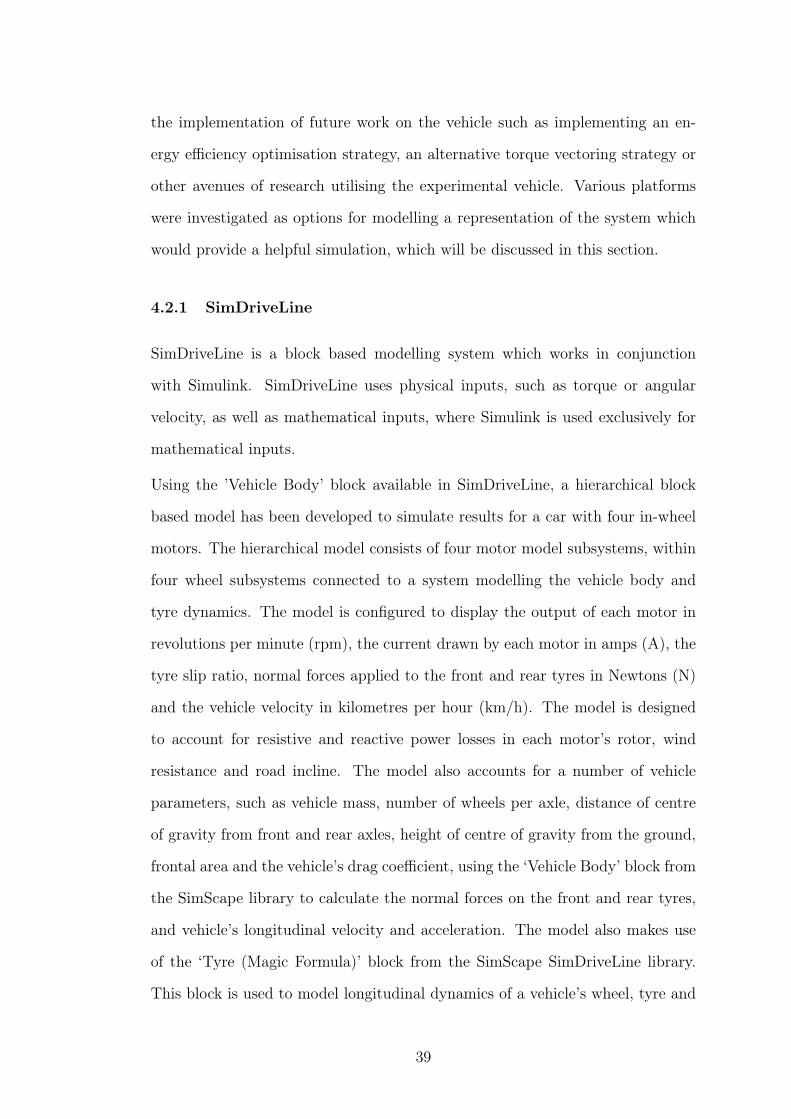
the implementation of future work on the vehicle such as implementing an en-

ergy efficiency optimisation strategy, an alternative torque vectoring strategy or

other avenues of research utilising the experimental vehicle. Various platforms

were investigated as options for modelling a representation of the system which

would provide a helpful simulation, which will be discussed in this section.

4.2.1 SimDriveLine

SimDriveLine is a block based modelling system which works in conjunction

with Simulink. SimDriveLine uses physical inputs, such as torque or angular

velocity, as well as mathematical inputs, where Simulink is used exclusively for

mathematical inputs.

Using the ’Vehicle Body’ block available in SimDriveLine, a hierarchical block

based model has been developed to simulate results for a car with four in-wheel

motors. The hierarchical model consists of four motor model subsystems, within

four wheel subsystems connected to a system modelling the vehicle body and

tyre dynamics. The model is configured to display the output of each motor in

revolutions per minute (rpm), the current drawn by each motor in amps (A), the

tyre slip ratio, normal forces applied to the front and rear tyres in Newtons (N)

and the vehicle velocity in kilometres per hour (km/h). The model is designed

to account for resistive and reactive power losses in each motor’s rotor, wind

resistance and road incline. The model also accounts for a number of vehicle

parameters, such as vehicle mass, number of wheels per axle, distance of centre

of gravity from front and rear axles, height of centre of gravity from the ground,

frontal area and the vehicle’s drag coefficient, using the ‘Vehicle Body’ block from

the SimScape library to calculate the normal forces on the front and rear tyres,

and vehicle’s longitudinal velocity and acceleration. The model also makes use

of the ‘Tyre (Magic Formula)’ block from the SimScape SimDriveLine library.

This block is used to model longitudinal dynamics of a vehicle’s wheel, tyre and

39

axel and road contact using the Magic Formula [23]. Use of this block within the

model allows for measurement of tyre slip and longitudinal vehicle velocity.

Figure 4: Top level of SimDriveLine model of an electric ground vehicle with fourin-wheel motors.

Pictured in figure 4 is the top level of the block based model used to evaluate

the vehicle parameters listed above. Shown in figure 5 is the successive layer of

the model, detailing the relationship between the vehicle body block, Tyre Magic

Formula block, DC Motor models and power supply.

Using the model pictured in figure 5, values may be obtained such as discussed

above. The main limitation of using SimDriveLine to evaluate vehicle dynamics

however, is that it is for one dimensional evaluation i.e. the package can only

40

Figure 5: Base level of SimDriveLine model of an electric vehicle with four in-wheel motors.

account for longitudinal motion. To investigate other vehicle dynamic character-

istics relevant to implementing a DYC control strategy the lateral motion of the

vehicle must be taken into account. Although this package is helpful for evaluat-

ing certain parameters such as acceleration, braking, maximum vehicle velocity

and tyre slip, additional simulation packages are required to evaluate other im-

portant performance indicators such as yaw rate and side-slip angle, and inspect

the lateral performance of the vehicle in a two or three dimensional model.

41

4.2.2 Simscape/SimMechanics

Vehicle For the purpose of evaluating an electric ground vehicle with four in-

dependently actuated in-wheel motors, a vehicle dynamics testing simulation has

been arranged. The blocks available in MATLAB SimMechanics in conjunction

with MF-Tyre using the Delft Tyre standard implementation of the renowned

Pacejka Magic Formula were used to simulate an electric ground vehicle with four

independently actuated motors. The focus of this simulation is on combining the

measurement of key performance indicators relevant to implementing a torque

vectoring control strategy with the benefits of Simulink in testing control archi-

tectures in hardware and programming mode. The work presented in this section

will focus on a simulation platform developed using MATLAB SimMechanics,

with the intended use of investigating the vehicle dynamics of conceptual elec-

tric ground vehicles with individually actuated motors. Simscape/SimMechanics

was utilised to develop a three dimensional simulation for inspecting the relevant

vehicle dynamic properties and behaviour.

Figure 6: Comparison of the modelled vehicle in simulation and the experimentalvehicle.

The simulation platform is developed to provide a baseline electric ground ve-

hicle, in which higher level control-architectures can easily be implemented, in-

terchanged and evaluated for the design of distributed drive systems and torque

vectoring DYC control strategies. The platform allows for a visual representa-

tion of the electric ground vehicle, and inspection of relevant vehicle dynamics

42

through measuring key performance indicators, such as tyre normal force, slip

ratio, side-slip angle, yaw rate and rolling resistance over a series of commonly

used driving manoeuvres such as J-turn and line change manoeuvres.

In the development of this platform, the focus is on measuring the performance

of the vehicle’s response to steering input to evaluate the effectiveness of the

DYC solutions being evaluated. The platform is not intended for the use of

vehicle body design characteristics related to the aerodynamics of the vehicle.

Therefore this platform is not intended for the use of measuring characteristics

related to vehicle body design such as wind resistance and drag coefficient, and

has been simplified to satisfy the requirements involved in developing a torque

distribution or energy efficiency strategy. As such, the model has been simplified

to include a visual representation of the vehicle containing a single point of inertia

taken from the vehicles centre of gravity. However, to maintain robustness of the

platform certain vehicle properties relevant to this area of design and research

remain adjustable. The position of the centre of gravity and the magnitude of the

inertia are both adjustable so that each system can be configured to accurately

reflect the needs of the current project. Similarly, vehicle body parameters which

affect vehicle performance are also adjustable. The vehicle length and wheel base

are also adjustable, in conjunction with the vehicle mass, adjusting these values

can be used to allow for the platform to make accurate calculations pertaining

the performance indicators of a range of vehicles, adding to the robustness of

the platform. All of these parameters are arranged into an accompanying script,

which runs at the startup of the simulation to provide the model with the relevant

vehicle properties and data required to perform.

The model discussed in this project was arranged from blocks available in the Sim-

scape library and the Delft Tyre Model to resemble an OAEGV (Over-Actuated

Electric Ground Vehicle) with in-wheel motors. The torque applied to each wheel

was modelled by a Permanent Magnet Synchronous Machine (PMSM). These

43

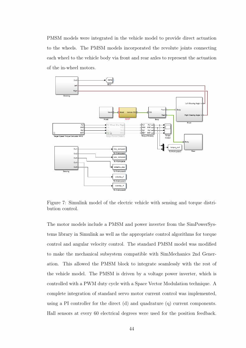
PMSM models were integrated in the vehicle model to provide direct actuation

to the wheels. The PMSM models incorporated the revolute joints connecting

each wheel to the vehicle body via front and rear axles to represent the actuation

of the in-wheel motors.

Figure 7: Simulink model of the electric vehicle with sensing and torque distri-bution control.

The motor models include a PMSM and power inverter from the SimPowerSys-

tems library in Simulink as well as the appropriate control algorithms for torque

control and angular velocity control. The standard PMSM model was modified

to make the mechanical subsystem compatible with SimMechanics 2nd Gener-

ation. This allowed the PMSM block to integrate seamlessly with the rest of

the vehicle model. The PMSM is driven by a voltage power inverter, which is

controlled with a PWM duty cycle with a Space Vector Modulation technique. A

complete integration of standard servo motor current control was implemented,

using a PI controller for the direct (d) and quadrature (q) current components.

Hall sensors at every 60 electrical degrees were used for the position feedback.

44

Figure 8: Flow diagram detailing the layout of the Simulink model of the electricvehicle.

The model also contains a low-fidelity variant of the motor model, which can be

interchanged for examining vehicle properties where the type of motor is not es-

sential to the outcome of the results. This is included for the purpose of reducing

compilation and simulation time to streamline processes of testing where several

iterations of running simulations are required.

As each wheel is powered with an in-wheel motor, the inertia parameter of the

motor and the vehicle body are taken into account to reflect the distribution of

sprung and un-sprung mass in the vehicle.

The end result of this work is a functional model and simulation of an OAEGV.

The model has the capability of inspecting torque demand and response to torque

input and vehicle dynamics response to steering inputs when undertaking perfor-

mance evaluation maneouvers. In addition to this, the developed model serves

as a framework suitable for implementation of OAEGVs with higher-level DYCs

containing control architectures for active drive solutions with hardware in the

loop capabilities.

45

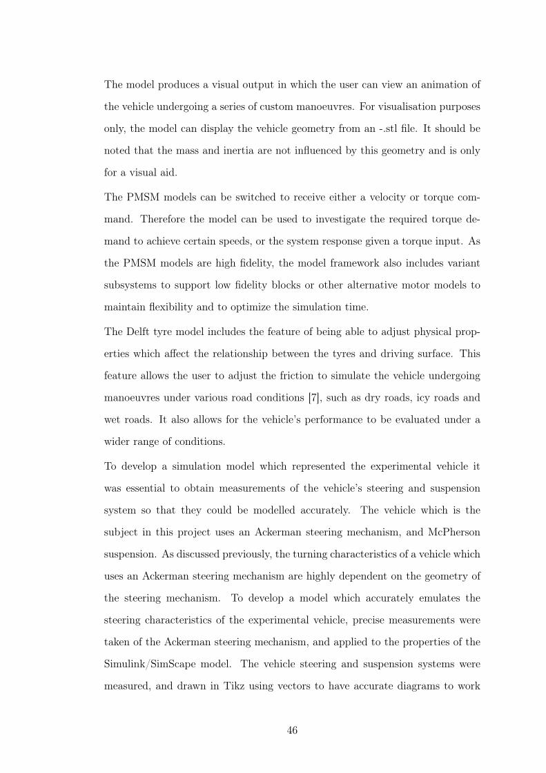
The model produces a visual output in which the user can view an animation of

the vehicle undergoing a series of custom manoeuvres. For visualisation purposes

only, the model can display the vehicle geometry from an -.stl file. It should be

noted that the mass and inertia are not influenced by this geometry and is only

for a visual aid.

The PMSM models can be switched to receive either a velocity or torque com-

mand. Therefore the model can be used to investigate the required torque de-

mand to achieve certain speeds, or the system response given a torque input. As

the PMSM models are high fidelity, the model framework also includes variant

subsystems to support low fidelity blocks or other alternative motor models to

maintain flexibility and to optimize the simulation time.

The Delft tyre model includes the feature of being able to adjust physical prop-

erties which affect the relationship between the tyres and driving surface. This

feature allows the user to adjust the friction to simulate the vehicle undergoing

manoeuvres under various road conditions [7], such as dry roads, icy roads and

wet roads. It also allows for the vehicle’s performance to be evaluated under a

wider range of conditions.

To develop a simulation model which represented the experimental vehicle it

was essential to obtain measurements of the vehicle’s steering and suspension

system so that they could be modelled accurately. The vehicle which is the

subject in this project uses an Ackerman steering mechanism, and McPherson

suspension. As discussed previously, the turning characteristics of a vehicle which

uses an Ackerman steering mechanism are highly dependent on the geometry of

the steering mechanism. To develop a model which accurately emulates the

steering characteristics of the experimental vehicle, precise measurements were

taken of the Ackerman steering mechanism, and applied to the properties of the

Simulink/SimScape model. The vehicle steering and suspension systems were

measured, and drawn in Tikz using vectors to have accurate diagrams to work

46

off of when modelling the system. The components comprising the front and rear

suspension and steering systems when sketched in Tikz appear as in figure 10.

The same concept of a low fidelity variant as applied to the motor model was

applied to the suspension and steering. Pictured in figure 9 is an example of a

low fidelity variant of the Ackerman steering mechanism for performing a J-turn

manoeuvre as modelled in Simulink.

Figure 9: Low fidelity implementation of Ackerman steering mechanism for per-forming a J-turn manoeuvre.

The overall composition of the front and rear suspension and steering systems

can be simplified into the diagrams presented in figures 11 and 12.

These diagrams were used as the basis for modelling the vehicle’s suspension and

steering to acheive an overall model for the vehicle in which vehicle behaviour

and dynamic response could be modelled and simulated.

The vehicle’s overall displacement, slip ratio, side-slip angle, yaw rate, longitudi-

nal, lateral and overall velocity and acceleration can be simulated. As discussed,

these are important results required to inspect the vehicle stability and effective-

ness of an implemented torque vectoring strategy.

Environment To evaluate the vehicle model developed in Simulink, certain

environmental aspects were modelled to provide a more wholistic approach to

investigating vehicle performance in real-life driving situations.

As discussed previously, split slippery surface and instantaneous split slippery

surface conditions are highly applicable to real-life driving situations, in account-

47

350mm

35mm70mm

35mm26mm

290mm

26mm49mm 32mm

350mm

30mm

240mm

19mm

290mm

25mm

25mm

80mm

38mm

xmm

25mm

Figure 10: Tikz diagrams of vehicle components.

ing for inconsistent road surface such as puddles, ice patches etc. on the road

surface where the individual tyres may perform differently. To account for this,

the tyre model was adapted to include split surface and instantaneous split sur-

face conditions. Shown in figure 13 is an example of the Simulink model used to

modify surface conditions to acheive split slippery surface or instantaneous split

slippery surface conditions when required. The longitudinal friction can now be

adjusted in the mask for each tyre to achieve split slippery surface conditions,

and step times are included to extend the model to accomodate instantaneous

split slippery surface conditions.

48

Figure 11: Tikz diagram of the layout of the vehicle’s front suspension system.

4.3 Data Acquisition and Estimation Techniques

The progression of available technology in recent years has allowed for the im-

plementation of measurement devices and estimation techniques to be applied to

receive fast and accurate data pertaining to the vehicle’s dynamic performance.

This data can be applied in real time, based on the controller design for the

vehicle’s torque vectoring control technique to provide feedback information to

actively improve the vehicle’s dynamic performance when compared to control

variables related to important perfomance indicators as mentioned previously.

Based on the design of the controller, feedback information which can be used to

improve vehicle performance can either be directly measured, or calculated using

estimation techniques to provide an indication of how the vehicle is performing

with respect to its target control variables. In this section the options explored

for the acquistion of relevant vehicle dynamics data will be discussed.

4.3.1 VBOX

The VBOX20SL Dual Antenna is a data logging unit which utilises two GPS

antennae to measure vehicle dynamics parameters. The VBOX20SL can be used

to measure and log relevant parameters to implementing a DYC strategy such as

49

Figure 12: Tikz diagram of the layout of the vehicle’s rear suspension system.

slip angle, pitch angle and yaw rate as well as longitudinal and lateral acceleration

and velocity. It is a compact unit, with a small size suited for implementation

on small vehicles such as cars and off road vehicles. The VBOX20SL module

makes use of two GPS signals to measure and calculate vehicle dynamics param-

eters. It is capable of logging at a rate of 20 Hz and has a positional accuracy

of 40 cm (standard) or 20 cm (optimised with a base station). The VBOX20SL

also includes two analogue outputs and two digital outputs, and a CAN Bus

interface [2].

For data logging the VBOX20SL has the option to log data onto an SD card or

connect to a computer via USB or RS232 serial port interface. This is a valuable

and useful tool for acquiring experimental data for evaluating the lateral and

longitudinal performance of the vehicle. The VBOX20SL can also log data in

real time, via analogue and/or digital outputs, as well as a CAN Bus interface

for logging data or use of Vbox input modules. For the purpose of implementing

the VBOX20SL module as a data acquisition device for a torque vectoring DYC

strategy these are useful features, as the output channels can be configured to

50

Figure 13: Modified mask for tyre models to extend vehicle testing to accomodatesplit and instantaneous split slippery surface conditions.

the required control variables for the DYC. For example, if yaw rate and side-

slip angle are to be utilised by the controller as control variables, the output

channels can be configured to yaw rate and side-slip angle, so that the controller

can receive these values in real time at 20 Hz to be utilised in the DYC strategy.

The capabilities of measuring velocity, acceleration and position are useful in the

process of validating the simulated model in the context of this project. This

module will allow for the collection of experimental data of the vehicle’s dynamic

performance, to be compared with that of the performance of the simulated

model. Vehicle performance manoeuvres can be performed on the experimental

vehicle and replicated in simulations to evaluate the consistency of the model.

Parameters such as the vehicle’s acceleration curve, top speed, and uncontrolled

yaw rate response to a given steering angle or steering manoeuvre can be assessed

and compared. As stated previously, it is important to have a realistic and

reliable model when utilising simulations as part of the design process, as such

51

Figure 14: VBOX20SL Dual Antenna Module. Image courtesy of [2].

the VBOX20SL is well suited for this purpose.

Vehicle side-slip angle is measured from a single point based on the positioning of

the antennae. The two antennae are assigned as “Antenna A” and “Antenna B”,

the VBOX20SL measures vehicle side-slip angle from the point where “Antenna

A” is attached to the vehicle. This is a limitation in a sense due to the fact

that the preferred method for some DYC controllers which utilise side-slip angle

as a control variable measure the side-slip angle of each tyre individually so

as to control vehicle side-slip more accurately. To implement a strategy where

side-slip is measured from each tyre, the VBOX20SL would not be suitable,

as it has insufficient antennae inputs to measure four differential GPS signals

simultaneously. However there are also strategies which utilise only one value for

side-slip angle measured from the vehicle’s centre of mass [58] which would only

require two antennae to implement. Using a strategy such as this, the VBOX20SL

module could be implemented into a feedback loop for a controller implementing

a similar DYC strategy.

Due to the capability of the VBOX20SL module to output side-slip angle and yaw

rate simultaneously, theoretically this module could be implemented in the use

of a DYC strategy based on controlling side-slip angle, yaw rate or an integrated

controller utilising both side-slip angle and yaw rate as control variables. The

VBOX20SL is useful for both acquisition of experimental data and for use in

measurement of vehicle dynamics parameters in implementing a DYC strategy.

52

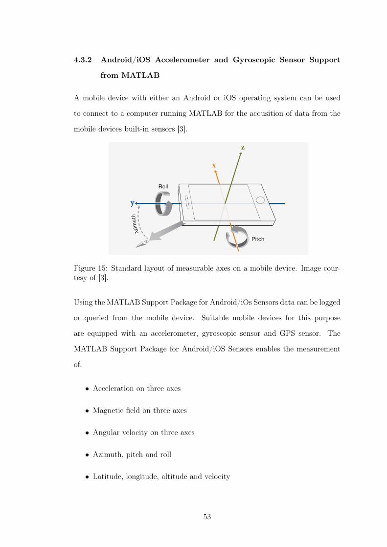
4.3.2 Android/iOS Accelerometer and Gyroscopic Sensor Support

from MATLAB

A mobile device with either an Android or iOS operating system can be used

to connect to a computer running MATLAB for the acqusition of data from the

mobile devices built-in sensors [3].

Figure 15: Standard layout of measurable axes on a mobile device. Image cour-tesy of [3].

Using the MATLAB Support Package for Android/iOs Sensors data can be logged

or queried from the mobile device. Suitable mobile devices for this purpose

are equipped with an accelerometer, gyroscopic sensor and GPS sensor. The

MATLAB Support Package for Android/iOS Sensors enables the measurement

of:

• Acceleration on three axes

• Magnetic field on three axes

• Angular velocity on three axes

• Azimuth, pitch and roll

• Latitude, longitude, altitude and velocity

53

This system operates by transmitting data between a computer running MAT-

LAB and a mobile device running MATLAB Mobile. The values which are to

be recorded can be controlled from either end, either from the MATLAB Mobile

GUI or by sending commands from the MATLAB terminal once a connection has

been established, to enable or disable sensors and logging.

Figure 16: Graphical user interface for Android/iOs Sensor Support on MATLABMobile. Image courtesy of [3].

A limitation is encountered, as this system only accomodates the logging of data

to a computer running MATLAB. There is no simple solution for using any of

the data acquired in real time which would not require the construction of a

custom hardware system, therefore it would be impractical to implement this

system as a means of acquiring data to be used as feedback information for a

controller as part of a DYC strategy. The disadvantages of using the inbuilt

sensors in a mobile device listed here can be overcome however, through use

of a gyroscopic sensor. Gyroscopic sensors can be purchased and integrated

into physical systems as required, and vary in accuracy and sensitivity based on

54

price. However, the usefulness of this system should not be overlooked. This

system is useful for evaluating vehicle performance, and has use in confirming

the accuracy of other measurement systems or validate the performance of the

simulated model. The process of establishing the link and using the mobile device

to log data is a quick and simple means for logging important vehicle dynamics

data. As discussed above, integrating simulations into the design process is only

beneficial if the simulation is an accurate reflection of the real life system, and

as such the MATLAB Support Package for Android/iOs sensors is useful for this

purpose. The accuracy of the sensors is dependent on the specifications of the

mobile device being utilised.

4.3.3 Motor Controller

Certain information, such as the motor’s angular velocity, can be requested using

through the CAN bus. The motor controller can trasmist its angular velocity in

revolutions per minute to within integer accuracy. As such, this is a simple and

effective method for receiving data for the driven wheels of the vehicle’s angular

velocity. As established previously, angular velocity of the wheels is required for

calculating certain performance indicators such as longitudinal wheel slip.

4.3.4 Encoder

If the controller, when implemented is performing undesirably as a result of in-

nacurate values estimated for longitudinal slip, the possibility of installing an

encoder onto the driving wheels can be explored to record higher accuracy values

for the angular velocity of each wheel. A rotary encoder could be utilised to

receive information on the angular position of the driving wheels to determine

the angular velocity of each driving wheel. This data could be used in conjunc-

tion with information acquired through other means measuring the velocity of

the vehicle to estimate values for longitudinal slip. With vehicle velocity and the

55

angular velocity of each driving wheel measured, it is possible to calculate the

longitudinal slip ratio for each wheel of the vehicle using equation (3).

Figure 17: Rotary encoder employed for measuring steering wheel angle in theexperimental vehicle.

Additionally, the rotary encoder is a useful tool for measuring steering wheel

angle. As the steering wheel angle is an important factor in altering the course

of the vehicle’s motion, it is necessary to measure the steering wheel angle when

performing vehicle dynamics testing. Additionally, many DYC strategies require

the measurement of the steering wheel angle as part of their algorithms for vehicle

control. A rotary encoder was included in the vehicle modifications, by securing

it parallel to the steering column with a shaft equal in diameter to the steering

column, and linking with a pulley. To enable real time measurement so as to be

useful for the purpose of both data logging and in the implementation of a DYC

strategy, the encoder is connected to the CAN bus.

4.3.5 Controller Area Network (CAN) Bus

A Controller Area Network (CAN) bus is utilised within this experimental vehicle

for consolodated, real-time transmission of critical data between vehicle systems.

The CAN bus is characterised by a maximum signalling rate of 1 megabit per

second, and unlike networks such as Ethernet or USB a CAN bus sends data in

short messages over the entire network to provide consistent data to the whole

56

system [59]. All of the sensor data acquired from the experimental vehicle is

to be broadcasted over the CAN bus. This is to ensure that all of the data

critical to implementing a torque vectoring control strategy or for inspecting

vehicle dynamics performance can be accessed from a single source and maintain

a consistent time stamp for ease of analysing data.

4.4 Summary

Taking into account all of the data acquistion devices available to the project and

the benefits they could provide, a final setup was decided upon and implemented

on the experimental vehicle. A CAN bus interface was implemented to provide

a single point of data acquistion, to allow for coallated data to be available from

a single unit and consistently timestamped. A laptop running Matlab is utilised

to receive the data on the CAN bus and send commands to request data when

required from the sensors in use. A rotary encoder was used to measure and record

steering wheel angle, as described previously by securing the unit parallel to the

steering column. The VBOX20SL was also implemented due to its versatility and

capability of measuring several important performance indicators, such as vehicle

speed, side-slip angle and yaw rate. The motor controllers in use were utilised

to obtain measurements for the angular velocity of each driven wheel, which

can in turn be used to calculate longitudinal wheel slip. A current sensor was

utilised to measure the current being delivered to the motor. By enabling current

measurement it is possible to calculate the torque transmitted by utilising other

measured variables such as the wheel radius and angular velocity of the wheel.

All of the sensors included are interfaced via the CAN bus.

57

5 Controller Definitions and Simulated Results

In this section the process and methods involved in developing and implementing

appropriate torque vectoring control strategies will be discussed, along with an

evaluation of the effectiveness of the strategies investigated through use of simu-

lations. Torque vectoring strategies will be assessed and compared based on their

feasibility to implement in hardware, potential to improve vehicle performance

and practicality of acquiring required feedback information as well as the poten-

tial to improve vehicle dynamics performance based on their simulated outcome.

The torque vectoring control strategies presented in this chapter are designed for

controlling either yaw rate or longitudinal performance and will be divided into

relevant subsections.

5.1 Longitudinal Wheel Slip Regulation DYC for Front-

Wheel Drive Electric Vehicle Controller Definition

The development of strategies pertaining to improving the lateral performance

via yaw rate control of the vehicle will be discussed in this section of the paper.

Longitudinal wheel slip regulation has been utilised in previous work as a means

of traction control for front-wheel drive internal combustion engine vehicles to

address the issue of traction force distribution between the wheels of a driving

axel [1]. A control algorithm is presented, based on implementation for internal

combustion engine vehicles with non-conventional differentials. The full set of

control algorithms set out by Doniselli et. al. are expressed as follows:

Δλ = λFL − λFR (30)

∆λ∗ = k1(r −vxδ

l) (31)

Mc = k2(∆λ∗ −∆λ) (32)

58

ML =M

2+MckL (33)

MR =M

2−MckR (34)

kL =1

|SL|+ 1(35)

kR =1

|SR|+ 1(36)

Where l is wheel base, r is yaw rate, δ is steering angle, vx is vehicle longitudinal

velocity, λ is the slip ratio, λ∗ is the desired slip ratio, Mcis the corrective torque,

k1and k2 are design parameters, MLand MRrepresent the torque delivered to the

left and right hand side driving wheels respectively, kLand kRare functions of the

slip ratio of the left and right wheels, SL and SR respectively [1]. The layout

for the controller proposed by Doniselli et. al. is as discussed previously in the

literature review.

The wheel slip regulation method proposed by Doniselli et. al. makes uses of dif-

ferentials to distribute torque between the left and right hand side driving wheels

of a two wheel-drive, front wheel-drive vehicle for improved traction control. The

limitation incurred as a result of relying on a single internal combustion engine

to deliver varying torque signals is identified by the author, however technolog-

ical availability at the time did not allow for a solution such as indepdendently

actuated in-wheel motors to deliver differential torque signals to the vehicle’s

driving wheels. Exploring the beneftits of in-wheel motor technology when ap-

plied to this strategy is addressed in this section. In-wheel motors, as opposed

to active differentials offer faster and more precise torque distribution as well as

the capability to deliver torque in forward and reverse directions [7]. As part

of this study, adapting this traction control method and modifying the control

law for use as a DYC strategy for improving vehicle performance of EVs with

IAIWM was undertaken. The controller presented in this section investigates

adapting this traction control method for use as a DYC strategy by modifying

59

the control law to accomodate the use of in-wheel motors and explore the ben-

efits they provide. The controller proposed in this section also investigates the

effects of extending the solution so that the algorithm can be applied to four-

wheel drive vehicles with independently actuated in-wheel motors. Additionally,

further improvement to the controller is investigated by implementing differen-

tial and integral gain terms to the controller. Using the simulation framework

developed as a platform for investigation, the modified control laws are modelled

and implemented using Simulink to investigate the validity of these control laws

as a DYC strategy.

The first step of extending on the control strategy set out by Doniselli et. al. [1]

was to apply the control law to an electric vehicle with independently actuated

in-wheel motors, as opposed to an internal combustion engine vehicle with active

torque distribution. It is expected that the strategy should be more effective

based on the advantages that the use of in-wheel motors offer [7]. For initial

investigation, the control algorithms presented by Doniselli et. al. [1] were imple-

mented in Simulink on the vehicle model for some indication of how effective this

strategy would be on a front-wheel-drive electric vehicle with two independently

actuated in-wheel motors.

The control architecture for the in-wheel motor design required some alterations

to translate the concept set out by Doniselli et. al. from an internal combustion

engine vehicle to an electric vehicle with in-wheel motors. The original controller

makes use of an input torque from the motor, which is divided and delivered to the

two driving wheels via a differential based on the feedback information obtained

from the controller. The baseline vehicle implemented in Simulink consists of a

top level controller to deliver the torque to each of the two motors driving the

front wheels of the vehicle, with a PID feedback loop to simulate the driver’s

throttle command to control velocity.

In this loop, the vehicle’s forward (longitudinal) velocity is used as the control

60

Figure 18: Simulink diagram of subsystem for generating a reference torque signalto simulate the driver’s input from the acceleration pedal.

variable and is used to deliver an even torque signal to each of the vehicles driving

wheels. This controller is not intended as a method of DYC implementation, but

rather as a modelling solution to produce a driving torque signal for basic motion

in place of a throttle command from the acceleration pedal by the driver. As

the original algorithm accounted for the torque delivery from a single source (the

internal combustion engine) and this implementation makes use of two sources for

torque delivery (two in-wheel motors) equations (33) and (34) can be substituted

for:

ML = TL +MckL (37)

MR = TR −MckL (38)

Where all terms are as previously expressed, with the exception of TLand TR

which represent the torque delivered to the front left and front right wheels

respectively by the velocity controller, replacing M2

as the torque split is no

longer required as a result of the driving torque being delivered from independent

sources.

The result of this work was a simulated implementation of the wheel slip regula-

tion control law set out by Doniselli et. al. adapted for use as a DYC strategy on

61

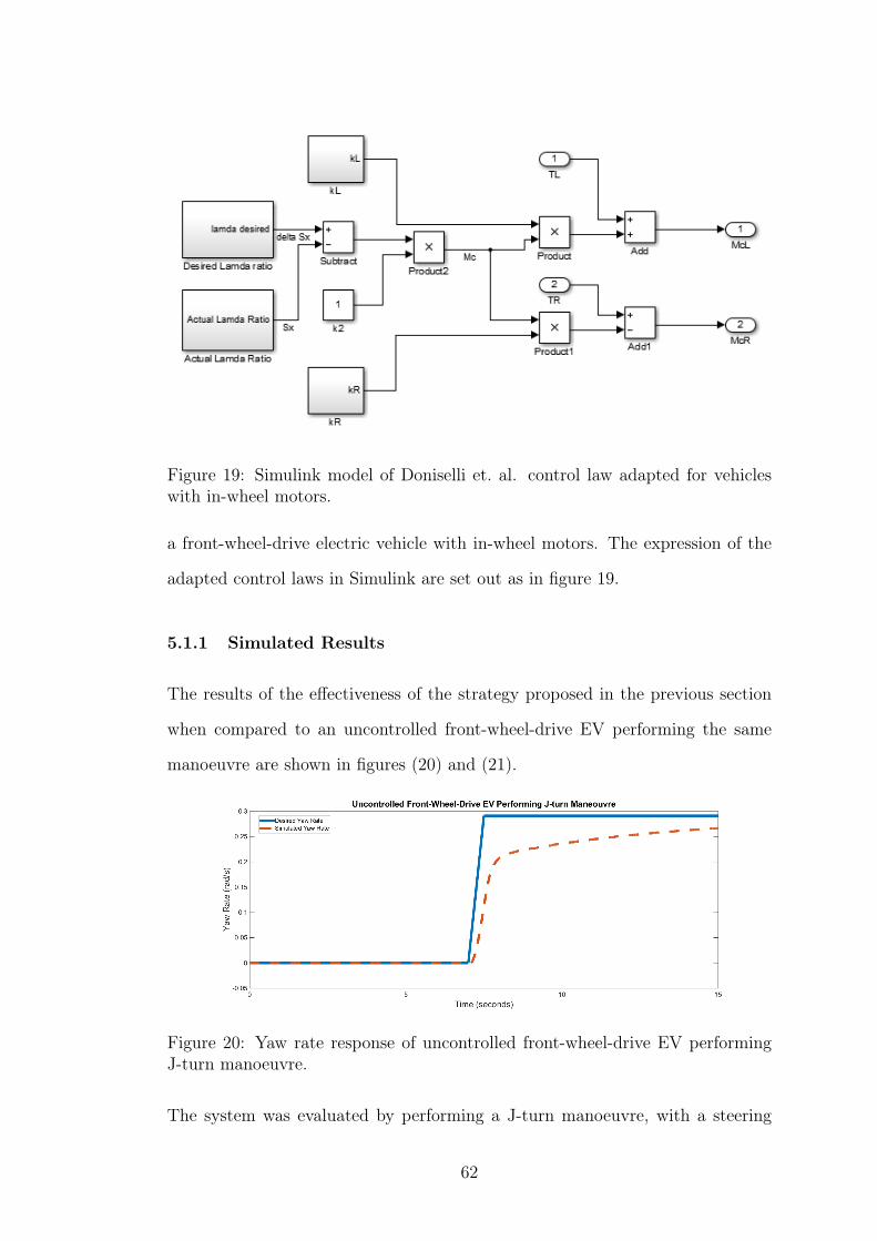
Figure 19: Simulink model of Doniselli et. al. control law adapted for vehicleswith in-wheel motors.

a front-wheel-drive electric vehicle with in-wheel motors. The expression of the

adapted control laws in Simulink are set out as in figure 19.

5.1.1 Simulated Results

The results of the effectiveness of the strategy proposed in the previous section

when compared to an uncontrolled front-wheel-drive EV performing the same

manoeuvre are shown in figures (20) and (21).

Figure 20: Yaw rate response of uncontrolled front-wheel-drive EV performingJ-turn manoeuvre.

The system was evaluated by performing a J-turn manoeuvre, with a steering

62

Figure 21: Yaw rate response of longitudinal wheel slip regulation algorithmadapted for front-wheel-drive EV with in-wheel motors performing a J-turn ma-noeuvre.

angle input of 6 degrees at time t = 6 s. As demonstrated by the results in

figure (20) and figure (21) there is a increased steady state yaw rate error when

compared to the uncontrolled system. Even when tuning the design parameters

(torque scaling and gain) for optimal results for a specific manoeuvre, the system

displays a slow response to steering input and maintains a significant steady state

error. In this case, using this particular method of control, the steering behaviour

is affected negatively. It is noteworthy however that the controller did function to

eliminate wheel slip from occuring on all tyres excluding the front-left tyre, which

still experienced approximately equal wheel slip to the uncontrolled system, as

shown in figures (22) and (23). The reduced wheel slip is indicative of reduced

loss of traciton, which in turn is an indication of improved vehicle stability and

safety. So although in this case there was no improvement in yaw rate response,

the controller did serve to reduce traction loss when performing the manoeuvre

and contribute to the vehicle’s overall stability and safety.

5.2 Longitudinal Wheel Slip Regulation for Electric Vehi-

cle with Four IAIWM Controller Definition

The next step in extending this DYC strategy was to investigate the effects of lon-

gitudinal wheel slip regulation when applied to vehicles with four independently

63

Figure 22: Uncontrolled longitudinal wheel-slip for front-wheel-drive EV (simu-lated).

actuated in-wheel motors. As the original control algorithms set out by Doniselli

et. al. were intended for use on an internal combustion engine vehicle with a

single source of torque delivery, yet again the algorithms had to be modified

to accomodate the four in-wheel motor vehicle system. In the four-wheel-drive

implementation wheel slip on all four wheels can be regulated, and used to gener-

ate corrective yaw moments as opposed to the two-wheel-drive implementations

previously discussed. The control law was modified to accomodate the feedback

information of wheel slip from all four wheels, and to deliver a corrective yaw

moment via delivering torque signals to each of the four driving wheels instead

of two. The comparison of the difference in slip ratio between the left and right

driving wheels was extended to include both driving wheels on the left and right

hand sides of the vehicle, as opposed to only the front two wheels. The adapta-

tion of this control law for a four-wheel drive electric vehicle with independently

actuated in-wheel motors is expressed in the following paragraphs. The measured

longitudinal slip ratio difference is modified to represent the total difference in

wheel slip between all driving wheels on the left and right hand sides of the ve-

hicle. The modified expression for obtaining the measured longitudinal slip ratio

64

Figure 23: Controlled longitudinal wheel-slip for front-wheel-drive EV (simu-lated).

difference is expressed in equation 39:

∆λ = λFL + λRL − λFR − λRR (39)

Where ∆λ represents the longitudinal slip ratio between left and right hand side

driving wheels of the vehicle, λFL, λRL, λFRand λRR represent the longitudinal

wheel slip of the front left, rear left, front right and rear left wheels respectively.

Including this expression as part of the control law adds to the robustness of

the model. As this value scales the magnitude of the error function, it serves as

a rudamental form of adaptively tuning the proportional gain of the controller.

Consequently, the functions kL and kR are extended to represent terms for all

four driving wheels, and become kFL, kFR, kRL and kRR expressed as:

kFL =1

|SFL|+ 1(40)

kFR =1

|SFR|+ 1(41)

kRL =1

|SRL|+ 1(42)

65

kRR =1

|SRR|+ 1(43)

Equations (40)through (43) represent a simple function to limit output torque

delivered to the motors to prevent excessive wheel slip, by multiplying the cor-

rective torque delivered to each wheel by their respective kij value. When wheel

slip for a given wheel, λij is a small value close to zero, kij will be close to one, re-

sulting in minimal compensation to the torque signal. Conversely, if λij happens

to a be a large negative or positive value this will result in a reduced value for kij

resulting in a reduction in torque delivered to that particular wheel. These terms

are extended to include all four wheels in the adapated design which reduce the

torque signal sent to each wheel when longitudinal wheel slip is detected, in an

effort to restrict excessive wheel slip from occurring.

This controller calculates the error between the desired yaw rate, rd, calculated

using equation (11) and the measured yaw rate, r, and scales this error signal

based on the longitudinal slip ratio difference between the left and right hand

side wheels, ∆λ, as expressed by equation (39). The controller design allows for

design factor k1, which serves as a proportional gain factor for scaling the error

signal. As such, the error function is expressed as:

Mc = k1(rd − r)− (∆λ) (44)

The following relationships represent how the system is adapted to an electric

vehicle with four independently actuated in-wheel moments. As shown by the

following expressions, the corrective yaw moment is delivered to the four driving

wheels, via four seperate torque signals. Each signal is a result of the scaled error

function comprised of yaw rate error and slip ratio difference (Mc)

MFL = TFL − k2MckFL (45)

MFR = TFR + k2MckFR (46)

66

MRL = TRL − k2MckRL (47)

MRR = TRR + k2MckRR (48)

The system when modelled in Simulink is pictured in figure 24.

Figure 24: Simulink model of longitudinal slip ratio (Doniselli et. al.) control lawextended to vehicles with four in-wheel motors.

5.2.1 Simulated Results

After extending the strategy to vehicles utilising four independently actuated in-

wheel motors, the system was evaluated. As the main objective of this thesis is

to improve vehicle stability and control, the effectiveness of the controller was

evaluated in terms of minimising yaw rate error. The system was evaluated using

a J-turn manoeuvre initially, and compared against a vehicle without yaw rate

control performing the same manoeuvre. The results of a step steer manoeuvre,

with a steering input of 6 degrees at time t = 7 s and vehicle speed of 20 km/h

for the uncontrolled and controlled vehicle are shown in the figures 25 and 26.

As demonstrated by the results in figure 26, the rise time is reduced in the

controlled system, indicating a system which is more responsive to steering input.

There is no overshoot evident, however there is a steady state error occurring. The

67

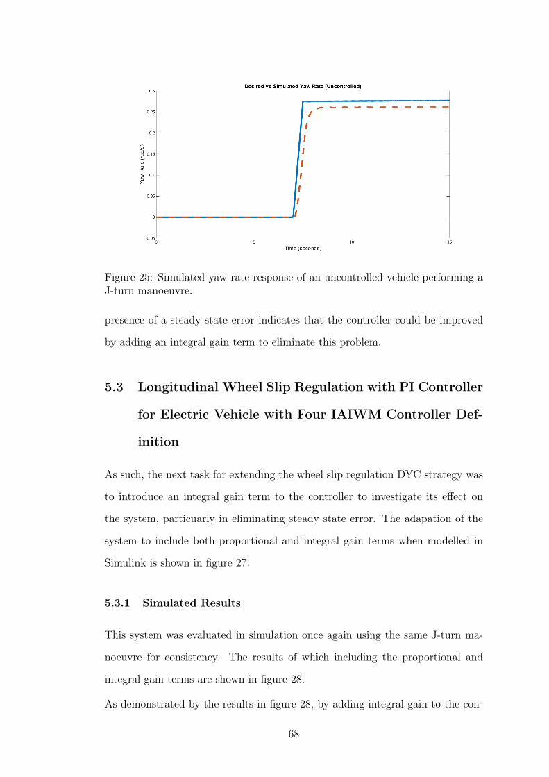
Figure 25: Simulated yaw rate response of an uncontrolled vehicle performing aJ-turn manoeuvre.

presence of a steady state error indicates that the controller could be improved

by adding an integral gain term to eliminate this problem.

5.3 Longitudinal Wheel Slip Regulation with PI Controller

for Electric Vehicle with Four IAIWM Controller Def-

inition

As such, the next task for extending the wheel slip regulation DYC strategy was

to introduce an integral gain term to the controller to investigate its effect on

the system, particuarly in eliminating steady state error. The adapation of the

system to include both proportional and integral gain terms when modelled in

Simulink is shown in figure 27.

5.3.1 Simulated Results

This system was evaluated in simulation once again using the same J-turn ma-

noeuvre for consistency. The results of which including the proportional and

integral gain terms are shown in figure 28.

As demonstrated by the results in figure 28, by adding integral gain to the con-

68

Figure 26: Simulated yaw rate response of vehicle with four IAIWM and longi-tudinal slip ratio control performing a J-turn manoeuvre

troller, the steady state error is eliminated with zero overshoot, and maintains

a reasonable response time. By examining the wheel-slip exhibited by each tyre

in the simulation comparing the controlled and uncontrolled sytem response to a

J-turn manoeuvre, as shown in figures (29) and (30), increased positive wheel-slip

can be observed in the right hand side tyres, and increased negative wheel-slip

can be observed in the left hand side tyres. This is resultant of controller inver-

vention to regulate the wheel-slip difference between the left and right hand sides

to induce a corrective yaw moment for the vehicle.

For further consistency of results, the uncontrolled system was compared against

the PI controller in a lane change manoeuvre to evaluate the yaw rate response

of the system. The results of the uncontrolled system are shown in figure 31.

As shown by figure 31 these results indicate a delayed yaw rate response to

the steering input, lagging by almost 1 second. Additionally, the system is not

acheiving the peak values set out for target yaw rate. This indicates that the

driver’s perception of control of the vehicle in performing such a manoeuvre

would be reduced, resulting in a sluggish and unresponsive steering manoeuvre.

By including the controller proposed in this section with the same PI terms the

results for a line change manoeuvre are demonstrated in figure 32:

69

Figure 27: Simulink model of longitudinal slip ratio control law including pro-portional and integral gain terms.

As demonstrated by the results in figure 32 the system is a lot more responsive

to steering input. There is a significant reduction in lag, indicating a much more

responsive system with an increased sense of perceived control by the driver. The

lag in peak values is reduced from almost 1 second to approximately 0.06 seconds.

Additionally, the peak error values experienced in the line change manoeuvre are

approximately 1.3 rad/s, indicating a significant understeer characteristic during

cornering. This error is reduced in magnitude from approximately 1.3 rad/s to

0.015 rad/s with the controller in place, equating to a reduction of approximately

25% in magnitude of error, and a turning characteristic much closer to neutral

steer behaviour, resulting in improved stability, and perception of control by the

driver.

5.3.2 Summary

The strategy proposed in this section has demonstrated through simulations, us-

ing the framework established in Simscape, an improvement in yaw rate response

and reduction in steady state error when performing standard testing manoeu-

70

Figure 28: Simulated yaw rate response of system performing a J-turn manoeuvrewith proportional and integreal gain terms included.

Figure 29: Longitudinal wheel slip of each tyre for uncontrolled EV with fourIAIWM performing J-turn manoeuvre.

vres such as the J-turn and line change. The control law has been adapted to

compensate for the two or four sources of torque input (in the form of in-wheel

motors), as opposed to utilising a single source of torque input. Additionally, the

control law has been extended to utilise proportional and integral gains for the

further improvement of results as demonstrated in figure 27. Overall the simula-

tions indicate that the adaptation and implementation of these control laws can

be used to improve vehicle performance and stability.

The control strategy outlined in this section requires the measurement of lon-

gitudinal slip ratio and yaw rate to be implemented on a real life vehicle. To

obtain values for longitudinal slip ratio, one method involves calculation using

71

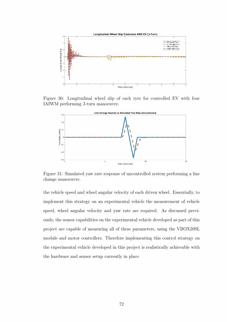
Figure 30: Longitudinal wheel slip of each tyre for controlled EV with fourIAIWM performing J-turn manoeuvre.

Figure 31: Simulated yaw rate response of uncontrolled system performing a linechange manoeuvre.

the vehicle speed and wheel angular velocity of each driven wheel. Essentially, to

implement this strategy on an experimental vehicle the measurement of vehicle

speed, wheel angular velocity and yaw rate are required. As discussed previ-

ously, the sensor capabilities on the experimental vehicle developed as part of this

project are capable of measuring all of these parameters, using the VBOX20SL

module and motor controllers. Therefore implementing this control strategy on

the experimental vehicle developed in this project is realistically achievable with

the hardware and sensor setup currently in place.

72

Figure 32: Simulated yaw rate response of system performing a line change ma-noeuvre with proportional and integreal gain terms included.

5.4 Longitudinal Performance Control

This section of the paper will include contributions made towards a control strat-

egy implemented for the purpose of improving the longitudinal performance of the

vehicle. This section presents a torque vectoring control strategy for an electric

ground vehicle with individually actuated in-wheel motors, and will outline the

investigation of the effects of controlling longitudinal wheel slip as a means for

improving vehicle longitudinal dynamics performance and stability under split

slippery surface conditions. The controller presented here is evaluated using

the simulation framework pertaining to relevant performance indicators used to

benchmark the effectiveness of the control strategy proposed.

The effects of undesired wheel slip can result in a loss of power delivered from

the driving wheels to the road surface, resulting in a loss of longitudinal acceler-

ation and disruptions to vehicle velocity [7]. As such a torque vectoring strategy

for maintaining longitudinal performance of the vehicle will be presented here.

Controller design based on longitudinal performance control is highly applicable

to real life driving situations. As discussed previously, under split slippery sur-

face conditions, road surface conditions are not always consistent and the friction

between each tyre and the road surface is not always the same. Split slippery

surface conditions can prove to be detrimental to vehicle stability due to un-

evenly distributed loss of traction, which may result in producing an undesired

73

yaw moment or loss of longitudinal velocity/acceleration.

The purpose of this controller is to regulate wheel slip to maintain longitudinal

acceleration and velocity by minimising disruptions to performance caused by

undesired wheel slip under slippery and split slippery surface conditions. The

controller proposed uses longitudinal wheel slip (λ) and vehicle longitudinal ve-

locity as the control variables for achieving this purpose. The algorithm for this

controller can be expressed as:

Δλ∗ = k(v∗x − vx) (49)

Where ∆λ∗ is the desired slip ratio, v∗x is the desired longitudinal vehicle velocity,

vx is the measured or actual longitudinal vehicle velocity and k is a proportional

gain term.

Figure 33: Application of control law expressed as a Simulink model.

The relevance of this DYC solution pertains to real life driving situations where

road surface conditions are not always optimal, and as such values for surface

friction coefficient may vary between each tyre and their respective road surface

contact area. For example, split-surface and instantaneous split-surface condi-

74

tions such as isolated puddles or ice patches on a road surface may result in

inconsistent performance of tyres, and varying performance between the tyres of

the vehicle at a given point in time, due to the composite road surface. As the

purpose of this controller is to maintain longitudinal acceleration and velocity and

minimise undesirable oscillations and disturbances to these values, longitudinal

vehicle velocity is adopted as the control variable for this purpose.

5.4.1 Simulated Results

Fig. 34 demonstrated that when travelling on split-slippery surface conditions the

uncontrolled system has a much slower acceleration curve, reaching the target

velocity at time t = 13 s as opposed to the controlled system, which through

redistribution of torque, managed to reach the target velocity at time t = 10 s.

This translates to a difference in average rate of acceleration of approximately

16 m/s2 or an increase of 29%.

Fig. 35 demonstrates that even with no steering angle present the yaw rate re-

sponse of the simulated vehicle under split-slippery surface conditions can affect

vehicle heading and cause undesired fluctuations in vehicle yaw rate. Conse-

quently, utilising the longitudinal slip regulation to maintain driving force, due

to the redistribution of torque being biased towards one side of the vehicle, this

can exasperate the effect on yaw rate that the vehicle experiences. Fig. 35 shows

the yaw rate error increases significantly, from a peak value of approximately

0.018 rad/s to 0.04 rad/s. This increase in yaw rate error is a consequence of the

controller correcting the loss of vehicle velocity due to low friction on some of the

vehicle’s tyres. The trade off exists as the controller can only improve either yaw

rate or velocity at any given point in time. Driver input however can be used to

account for the yaw rate error with steering input.

Fig. 35 demonstrates that even with no steering angle present the yaw rate re-

sponse of the simulated vehicle under split-slippery surface conditions can affect

75

Figure 34: Comparison of uncontrolled vehicle velocity under split-slippery sur-face conditions and controlled vehicle velocity under split-slippery surface condi-tions.

vehicle heading and cause undesired fluctuations in vehicle yaw rate. Conse-

quently, utilising the longitudinal slip regulation to maintain driving force, due

to the redistribution of torque being biased towards one side of the vehicle, this

can exasperate the effect on yaw rate that the vehicle experiences. Fig. 35 shows

the yaw rate error increases significantly, from a peak value of approximately

0.018 rad/s to 0.04 rad/s. This increase in yaw rate error is a consequence of the

controller correcting the loss of vehicle velocity due to low friction on some of the

vehicle’s tyres. The trade off exists as the controller can only improve either yaw

rate or velocity at any given point in time. Driver input however can be used to

account for the yaw rate error with steering input.

76

Figure 35: Comparison of the effect on vehicle yaw rate on split slippery surfaceconditions for straight line driving for uncontrolled and controlled systems.

5.5 Summary of Simulated Results

The DYC strategy based on longitudinal wheel slip ratio regulation was im-

plemented through simulations on the model of the experimental vehicle. The

control law as set out in equation (39) for four in-wheel motors and PI control

was evaluated performing a J-turn and line change manoeuvre to inspect the

system response. Firstly, the yaw rate response of the variations of control strat-

egy of the simulated vehicle will be compared and inspected here. The yaw rate

response of the uncontrolled system with front-wheel drive only can be seen in

figure 36.

By adjusting the system to simulate an electric vehicle with four in-wheel motors,

the results can be observed in figure 37.

As can be seen by figures 36 and 37, the introduction of four-wheel drive as

compared to front-wheel drive does with no control law in place has a minimal

77

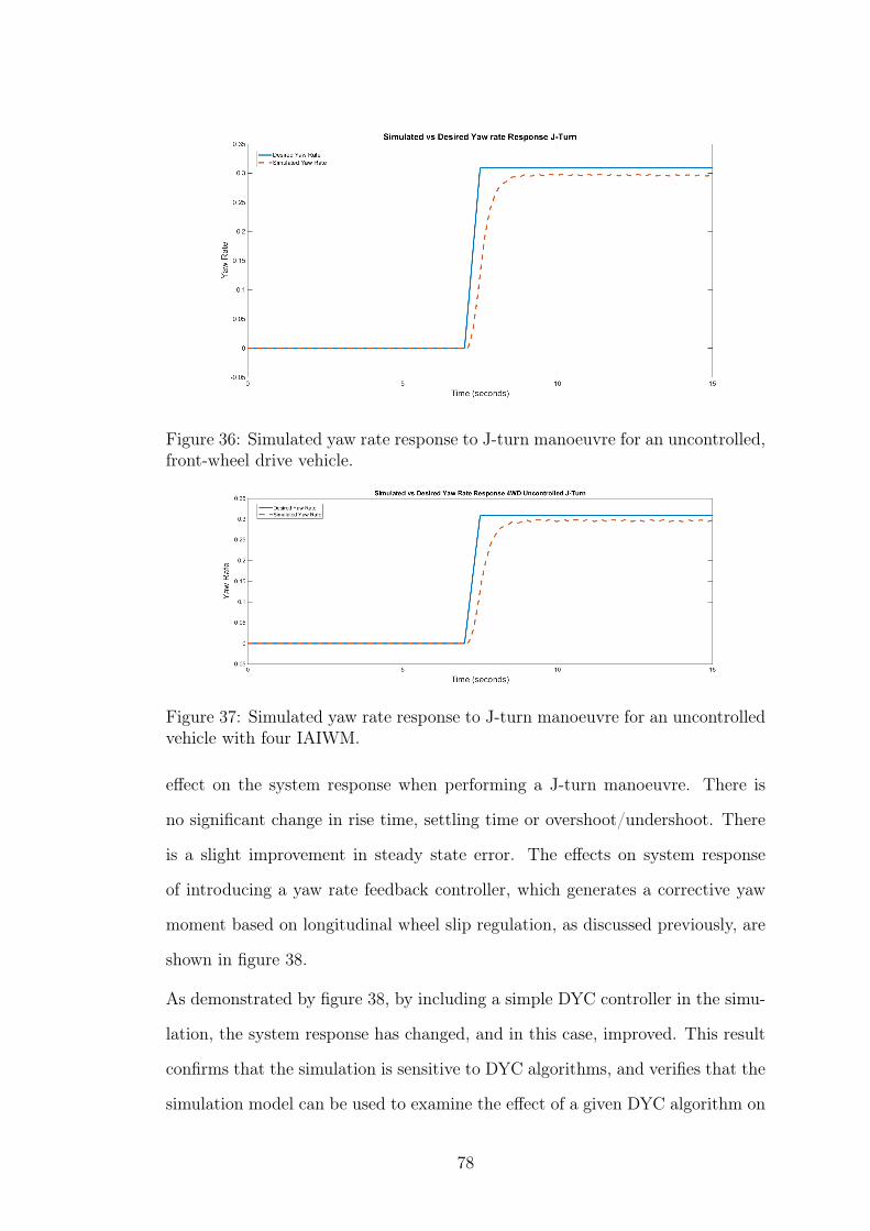
Figure 36: Simulated yaw rate response to J-turn manoeuvre for an uncontrolled,front-wheel drive vehicle.

Figure 37: Simulated yaw rate response to J-turn manoeuvre for an uncontrolledvehicle with four IAIWM.

effect on the system response when performing a J-turn manoeuvre. There is

no significant change in rise time, settling time or overshoot/undershoot. There

is a slight improvement in steady state error. The effects on system response

of introducing a yaw rate feedback controller, which generates a corrective yaw

moment based on longitudinal wheel slip regulation, as discussed previously, are

shown in figure 38.

As demonstrated by figure 38, by including a simple DYC controller in the simu-

lation, the system response has changed, and in this case, improved. This result

confirms that the simulation is sensitive to DYC algorithms, and verifies that the

simulation model can be used to examine the effect of a given DYC algorithm on

78

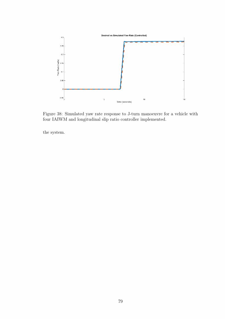
Figure 38: Simulated yaw rate response to J-turn manoeuvre for a vehicle withfour IAIWM and longitudinal slip ratio controller implemented.

the system.

79

6 Experimentally Acquired Results and Valida-

tion

This chapter will include a summary of experimentally obtained results and cal-

culations used for validating the simulated vehicle model. Methods of data acqui-

sition and estimation of useful information will also be included in this chapter.

A discussion of experimental results is included here. This section also includes a

review of the validation process of the simulation platform used to obtain results

and aid in the design process in this project.

6.1 Validation of Simulation Platform

This section will detail the process involved in verifying the validity of the sim-

ulation platform at use in the design and experimental process of this project.

There are many benefits of integrating simulation into the process of design and

experimentation. Simulating results can often be a lot more efficient in the de-

sign process as opposed to obtaining results experimentally. The design process

may call for multiple iterations of the experiment to be run, with varying pa-

rameters and values. As such the use of simulation can streamline this process

and allow for these design parameters to be easily manipulated. Additionally,

there are often inherent risks in performing experiments, especially in a scenario

such as this involving the operation of an electric vehicle performing cornering

manoeuvres. The risk of injury or damage to property can be reduced by running

tests in simulation, and minimising the number of experiments which need to be

performed. However if the simulation platform is an innacurate reflection of the

real life system, the controller design may be based on false or innacurate results

and function inneffectively. Therefore it is important to validate the reliability

and accuracy of the model before relying on it as a tool for design of real system

components.

80

The validity of the simulation output was verified initially through observation, by

inputting values and observing expected results. The simulation results indicate

a functional platform and will be discussed in the following section. A simple

torque vector control algorithm is to deliver different values of torque to either

side of the vehicle, inducing a yaw moment about the vehicle’s vertical axis.

This can assist the vehicle to turn, even when no steering angle is present. A

generic torque input of 150 Nm was applied to the left side wheels and 50 Nm

was applied to the right side wheels in the simulation, for a total of 400 Nm of

torque distributed across the four driving wheels. This was compared to an even

torque distribution of 400 Nm across the four driving wheels, with 100 Nm being

delivered to each wheel. The simulation results of the biased and unbiased torque

distribution are shown in figures 39 and 40.

Figure 39: Simulated system response of displacement over time to even torquedistribution.

Figure 40: Simulated system response of displacement over time to a biasedtorque distribution.

81

The results in figure 39 and figure 40 display the longitudinal and lateral displace-

ment of the vehicle given a steering angle of zero. The results are as expected,

displaying straight line motion for the evenly distributed driving torque, and a

deviation in path towards the right hand side of the vehicle when a torque bias

was induced with increased torque to the left hand side driving wheels, evident

as negative lateral displacement in figure 40.

The simulated results were also compared to theoretically calculated results to

verify the model’s validity. Firstly, the forward velocity (Vx) of each tyre was cal-

culated using the effective rolling radius (re) and angular speed (Ω0) as described

by equation (50) [23].

Vx = Ω0re (50)

Figure 41: Simulated and theoretically calculated forward velocity of the simu-lated vehicle model.

Figure 41 shows the comparison between the calculated results and the simulated

results of the forward velocity of the front left tyre given a constant torque signal.

As demonstrated by the results, the expected forward velocity of the vehicle is a

very close match to the simulation output, which is representative of a reliable

system.

As discussed previously, the CAN bus can be used to request the motor angular

velocity from the motor controller, however only to within 1rpm of accuracy.

82

Longitudinal wheel slip is used as feedback in some DYC strategies, and as such,

it needs to be determined if 1 rpm accuracy is sufficient for use in a feedback

loop to produce an effective result using a DYC controller. This was investigated

by quantizing the data in the simulation model to within 1 rpm accuracy for

wheel angular velocity, and calculating wheel slip. The results calculated were

compared against the results simulated from the MF-Tyre model, and used as

feedback in the proposed DYC strategy.

Figure 42: Comparison of simulated wheel slip acquired with unaltered and quan-tized data for wheel angular velocity.

As such, it was shown that the results calculated with the restrictions on ac-

curacy for measuring wheel angular velocity, did not have a signifcant effect on

the calculation of wheel slip. Both curves were representative of the same tyre

behaviour, and all values had a very small margin of error, to within approxi-

mately 0.02%. As such, the DYC strategy was implemented using both sources

for wheel slip feedback, and it was observed to have no effect on vehicle response

as both yaw rates were identical. As such, it has been validated that the wheel

slip which can be calculated from the measurements of wheel angular velocity

obtained from the motor controllers are within an acceptable range of accuracy

to implement a DYC strategy utilizing longitudinal wheel slip as feedback.

83

6.1.1 Experimentally Verified Results

Experimental data acquired from the various sensors previously discussed were

used to verify the simulation platform’s validity in representing the vehicle as

a real life system. Data acquired from the experimental vehicle’s sensors was

used to create a comparison between the simulated vehicle and the experimental

vehicle’s performance. Sensor data was used to create a torque signal and steer-

ing angle signal to be used as inputs to the simulation, and the outputs of the

simulation were compared to the sensor data acquired from the electric vehicle

to draw a comparison between the performance of the two systems.

As discussed previously, a rotary encoder attached to the steering wheel column

was used to obtain measurements for the steering wheel angle of the experimental

vehicle. The encoder was connected to the CAN bus so as to synchronise the

information registered with the other signals so as to obtain more meaningful

data for creating a wholistic representation of the vehicle manoeuvres completed

and the resultant performance indicators to be measured. The encoder used to

measure the steering wheel angle outputs data in “counts”. To convert this data

into a meaningful measurement the steering wheel angle had to be calibrated. The

steering angle was calibrated by turning the wheel for one or two full rotations,

and adding the number of counts received. The calibration was repeated several

times to ensure accuracy. The result of the calibration showed consistently that

two full revolutions were comprised of 4456 counts, and a single revolution of the

steering wheel was comprised of 2228 counts. Using this information, it could be

determined that 1 degrees was equal to approximately 6.18 counts.

A major performance indicator in investigating and evaluating vehicle control

and stability is the vehicle yaw rate. It is important to the have a means of

accurately measuring the yaw rate of the vehicle when implementing a DYC con-

troller, as many controller designs require the measured yaw rate of the vehicle

as a feedback signal. As such, it is necessary to ensure that the yaw rate response

84

of the simulated vehicle is reasonably consistent with that of the experimental

vehicle, to ensure that the yaw rate response induced by the controller in sim-

ulations is an accurate reflection of how the experimental vehicle will behave.

To validate the model’s yaw rate response was indeed an accurate reflection of

the experimental vehicle, a test was performed, in which both the experimen-

tal and simulated vehicle drove at a constant speed, and were given the same

steering input. Using the experimental vehicle and the method described above,

a line-change manoeuvre was performed with important performance indicators

being measured. Capturing the steering wheel position and torque output the

manoeuvre was recreated on the simulation, and the performance was compared.

The steering wheel angle and torque signals captured from the experiment and

used as inputs to the simulation can be seen in figures 43 and 44.

Figure 43: Steering wheel angle measured from encoder on experimental vehi-cle steering shaft and replicated signal built on Simulink for input to simulatedvehicle.

The vehicle’s yaw rate was the first performance indicator to be compared, be-

cause as established, controlling this variable is the major focus of a DYC con-

troller. As such, the result of the torque and steering signals recreated from

the measured values from the experimental vehicle when used as input to the

simulation can be inspected in figure 45.

After re-creating the torque and steering angles as input signals to the simulation,

the vehicle was observed to perform the line change manoeuvre in the simulation,

as performed earlier in the experimental vehicle. As recorded in figure 45 the

85

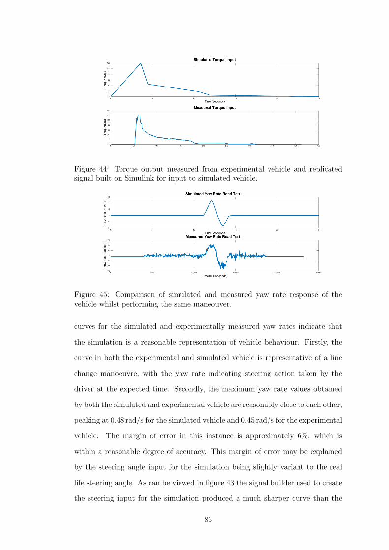
Figure 44: Torque output measured from experimental vehicle and replicatedsignal built on Simulink for input to simulated vehicle.

Figure 45: Comparison of simulated and measured yaw rate response of thevehicle whilst performing the same maneouver.

curves for the simulated and experimentally measured yaw rates indicate that

the simulation is a reasonable representation of vehicle behaviour. Firstly, the

curve in both the experimental and simulated vehicle is representative of a line

change manoeuvre, with the yaw rate indicating steering action taken by the

driver at the expected time. Secondly, the maximum yaw rate values obtained

by both the simulated and experimental vehicle are reasonably close to each other,

peaking at 0.48 rad/s for the simulated vehicle and 0.45 rad/s for the experimental

vehicle. The margin of error in this instance is approximately 6%, which is

within a reasonable degree of accuracy. This margin of error may be explained

by the steering angle input for the simulation being slightly variant to the real

life steering angle. As can be viewed in figure 43 the signal builder used to create

the steering input for the simulation produced a much sharper curve than the

86

steering input measured from the encoder on the experimental vehicle. This was

resultant in a slight variation in yaw rate, but overall still maintained a reasonably

accurate representation of what the steering input was. The simulated response

also produces a much “smoother” curve than the experimentally acquired yaw

rate response. This disturbance in the signal can be explained by the sensor on

the experimental vehicle is sensitive to several small oscillations in the yaw rate

of the vehicle, which the simulation is not subject to. For example, the road

surface in the simulation is evaluated as a smooth road surface, however in real

life experiments the road surface is not perfectly smoothe, so small oscillations

in yaw rate occur as a result of “road noise”. Seconly, there are vibrations within

the experimental vehicle, such as where the VBOX antennae are attached to the

vehicle as a result of the vehicle driving on a road surface which is not completely

smoothe. As a result of these vehicle vibrations, small oscillations in the yaw

rate are a consequence, which are recorded by the VBOX module. Thirdly, the

steering wheel input signal in Simulink allows for a “perfect” signal, i.e. the

output will be exactly what it is programmed to be, whereas in the experimental

vehicle, the steering wheel angle is controlled by human hands, and is therefore

subject to human error, resulting in slight variations to the steering wheel angle.

However as the peak values are within a reasonably close range (error values <

10%) and the curve is representative of the manoeuvre performed, the oscillations

can be disregarded to acquire a reasonably accurate respresentation of the yaw

rate response from the simulated electric vehicle.

The next measurable variable to compare was the vehicle velocity. It is important

that when given a similar torque input, the experimental vehicle and simulated

vehicle achieve a similar rate of acceleration and top speed, to verify that the per-

formance of the simulation is an accurate representation of the vehicle’s response

to torque input. The torque signals displayed in figure 44 represent the torque

delivered to the left front wheel of the experimental vehicle, and the signal used

to deliver torque to the front left wheel of the simulated vehicle. The measured

87

torque signal was calculated from measuring the current delivered from one of

the motor controllers to the front left motor. Due to the availbility of sensors

for the experiment, only one current signal could be measured, and the decision

to measure current on the left hand side motor is arbitrary. As no torque distri-

bution strategy for uneven torque signals is put in place here it is assumed that

both torque signals are equal to a reasonable extent in this experiment, as the

conditions for the simulation verification tests are treated as such, i.e. an identi-

cal torque signal is delivered to both the left and right hand side driving wheels.

The results of this experiment when comparing vehicle speed can be observed in

figure 46.

Figure 46: Comparison of absolute vehicle speed for the experimental and simu-lated vehicles.

As discussed above, a torque signal was created in Simulink signal builder and

distributed to the two front driving wheels of the simulated vehicle, based on the

torque calculated to be delivered to the experimental vehicle based on current

measurements. Examining the velocity of the experimental and simulated vehi-

cle, shown in figure 46 there is significant variation between the two curves during

the decceleration of the vehicle. This can be explained because the experimental

vehicle is at this stage, still equipped with mechanical brakes and there is no

sensor in place for measuring the braking force from the mechanical brakes. As a

result, at this stage the braking force acting on the vehicle cannot accurately be

measured, only the torque being delivered to the electric motors can be measured.

88

Consequently, this allows for a torque signal mapped from the motor current to

be used as torque input for the simulated vehicle, which does not account for

mechanical braking, hence the variation in vehicle speed when the experimen-

tal vehicle begins to deccelerate at approximately time t = 14 seconds. In the

simulation, the torque delivered tapers off, but without the input of a braking

force, the vehicle maintains forward velocity through its momentum. In future

work when recreating this experiment, an idealized brake torque or a model for

regenerative braking could be included. In this case however there was no means

of accurately measuring the braking force and applying it to the model, and as

the deceleration curve was not the focus of this investigation the braking torque

was not considered crucial.

The next aspect of the curve which requires analysis is the vehicle top speed. For

the simulated model to be an accurate representation of the experimental vehicle,

a similar top speed should be attained given a similar torque signal as input to

the motors. Comparing the experimentally obtained and simulated results, the

experimental vehicle reached a top speed of approximately 21 km/h. When given

the same torque input, the simulated vehicle reached a top speed of approximately

21.5 km/h. Comparing these two values, with an difference of 0.5 km/h the error

for top speed is apprximately 2.3%. This is within an reasonably small margin of

error and indicates an accurate representation of the experimental system through

a simulation in terms of top speed.

The final aspect of the curve to analyse is the rate of acceleration. It is important

to determine whether the rate of acceleration of the experimental vehicle and

simulated vehicle are reasonably similar (within ± 10%) given the same input

torque. Examining the curve at the time of acceleration, in this case from time

t = 0 seconds to time t = 10 seconds, the average rate of acceleration for the

experimental and simulated vehicles are calculated to be 1.90 m/s2 and 2.05 m/s2

respectively. This amounts to be a margin of error of approximately 7.9% for

89

average rate of acceleration. Again, this falls within a reasonable margin of

accuracy (within ± 10%) and is therefore determined to be a reasonably accurate

representation of the system. Certain factors may affect the accuracy of the

vehicle speed, such as wind resistance. Wind resistance can be adjusted in the

simulated model, by setting a value for the damping coefficient for the vehicle

centre of gravity in the six degree of freedom block which represents the vehicles

geometric centre of mass. This factor however will not always be completely

representative of the real life driving situation, as on different days, different

conditions are apparent, for example if the vehicle is facing a strong headwind the

acceleration and velocity will be slowed. Additionally, the variation in velocity

and acceleration may also be a result of slightly different sized tyres used on

the experimental vehicle and the simulated vehicle. The tyres available to the

experiment were of a slightly larger radius than those utilised in the simulation,

which is resultant in variant vehicle dynamic performance.

Figure 47: Comparison of simulated and experimentally acquired values for lon-gitudinal wheel slip of the front-left tyre.

As discussed previously, longitudinal wheel slip ratio is an important performance

indicator of vehicle dynamics, as it provides a strong indication of the traction

of the vehicle’s tyres and the road surface. Consequently, it is important to have

some form of sensor capabilities on the experimental vehicle which can allow for

the calculation of the vehicle’s longitudinal wheel slip for both analysing vehicle

performance and in the implementation of torque vectoring or traction control

90

strategies. Shown in figure 47 are the longitudinal wheel slip ratios acquired from

the simulated and experimental vehicles when performing the same manoeuvre.

The wheel slip on the experimental vehicle is obtained by measuring the driven

wheel’s angular velocity from the motor controller, using the radius of the tyre

as a measured constant, and the linear velocity of the vehicle using the VBOX

module. After measuring these values, the longitudinal wheel slip is calculated

using Equation 3. There is some variance between the simulated and measured

values for longitudinal wheel slip, this can be explained by the slight difference

in wheel radius. The simulated vehicle and experimental vehicle are both using

different sized wheels, hence resulting in a different result for wheel slip. Another

source of variance in values is the road surface friction. In the simulation, a

standard friciton coefficient of 1 is used to represent a normal dry road surface.

However, it cannot be determined if the road surface in the experimental trail

is completely consistent and there may be some increased or decreased friciton

at certain parts of the road surface, which will affect the longitudinal slip of the

tyres. Additionally, the motor controllers used on the experimental vehicle are

only capable of outputting angular velocity to integer accuracy (RPM). Tests

performed in the simulation mode in which the slip ratio was calculated using

wheel angular velocity measurements quantised to within integer accuracy were

compared to the default longitudinal wheel slip measurements. Results showed

that the quantisation of angular velocity measurements did not bear a detrimental

effect on the measurement of the wheel slip, or the performance of the control

strategy put in place. Given that, and since the results for wheel slip are relatively

close (maximum margin of error within 0.01%) it is assumed that this is an

acceptable method for obtaining longitudinal wheel slip ratio measurements for

use in a control strategy on the experimental vehicle.

As established, vehicle sideslip is another important performance indicator of ve-

hicle stability and control. Sideslip angle is often controlled as part of a DYC

strategy and as such, it is important that in this platform a means of measuring

91

and simulating vehicle sideslip is established. The VBOX20SL module was used

to obtain experimentally measured values for vehicle sideslip, with the antennae

positioned so that the point of measurement is to be taken from the vehicle cen-

tre of gravity (C.O.G.). Shown in figure 48 and figure 49 are the experimentally

measured and simulated sideslip respectively. The simulation and experimental

test were synchronised as outlined previously, with the torque and steering in-

puts to the simulated vehicle modelled based on the values measured from the

experimental vehicle to recreate the same manoeuvre performed under similar

conditions.

As shown by the results in figures 48 and 49 there appear to be more oscila-

tions in sideslip in the experimentally acquired data in figure 48. This can be

explained similarly to the oscilations in yaw rate, as vibrations which occur in

the experimental system due to vehicle vibrations and road noise are not evident

in the simulated model. The shape of the curve is a close match for both the ex-

perimental and simulated values, both reaching negative maximum and positive

maximum at approximately t = 12.5s and t = 14s for the experimental data and

at approximately t = 12s and t = 13.5s for the simulated model.

Figure 48: Experimentally measured sideslip measured from the vehicle centre ofgravity.

The slight time shift and discrepancy in magnitude is a result of the VBOX20SL

measuring the vehicle sideslip from the vehicle centre of gravity in the experi-

mental results, and in the simulation the sideslip was measured from the front

92

left and front right tyres. Figure 49 shows that the mangitude for sideslip is

greater on the outer wheel (initially the right wheel when turning left, and then

the left wheel when turning right) throughout the simulation. The positioning of

the sensors at different locations on the experimental and simulated vehicle will

result in a time shift due to being at a different displacement at any given time.

The magnitude also varies due to the placement of the sensors, as the same mag-

nitude of sideslip cannot be expected to be identical at different locations of the

vehicle. Examining the desired and actual yaw rate of the vehicle in figure 50 it

is evident that the vehicle is experiencing understeer turning characteristic. This

result maintains consistency with the output of the vehicle sidelip values being

higher in magnitude on the outer wheels during cornering, as this behaviour is

also indicative of understeer behaviour. The differennce in mangitude in vehicle

sideslip could also be explained by differing road surface conditions between the

simulated and experimental environment. Inconsistent road surface friction in

the real life driving situation may result in increased or reduced wheel slip and

this may be reflected in the results.

Figure 49: Simulated vehicle sideslip front left and front right tyres.

However, the the shape of the curve and magnitude of sideslip angle remains

consistent in both the simulation and experimental setup and given that in the

majority of cases, the reference value for vehicle sideslip is zero, for evaluation

in simulation and implementation using hardware both cases are useful. The

93

Figure 50: Desired and actual yaw rate of line change manoeuvre.

controller objective for sideslip control is consistent in both cases by reducing

the error to zero in the same direction and at the same point in time during the

manoeuvre.

94

7 Future Work and Conclusions

7.1 Future Work and Applications

Active steering, in which the angle of the vehicle’s wheels are controlled indepen-

dently of driver input or steering wheel angle is an option for future implemen-

tation on this project. Active steering can be applied to either the front, rear or

front and rear wheels of the vehicle [60, 61]. Active steering can be integrated

into a DYC strategy and has been shown to be a robust solution in terms of

conforming to desired yaw rate and side-slip angles, especially during changes in

road surface conditions and vehicle parameters such as cornering stiffness [62].

As such, the integration of an active steering solution to the DYC strategy is a

possible avenue of future research to pursue on the project which if implemented

correctly, could result in improved vehicle control and stability.

Similarly to active steering, four-wheel steering has been shown to be an effective

measure in eliminating vehicle side-slip, which as previously discussed is a major

contributor to reductions in vehicle stability [63]. As such, four-wheel steering

solutions are also a possible avenue of future research which can be undertaken

on this experimental vehicle to further improve vehicle stability and handling.

The implementation of which would involve extending the capabilities of both

the experimental vehicle and the simulation framework.

Given the environmental benefits of EGVs, improving the energy efficiency of

electric vehicles is a prominent area of research. A major limitation of EGVs

when compared to internal combustion engine vehicles is their range i.e. compar-

ing how far the vehicle can travel on a single charge as opposed to a tank of fuel.

The experimental vehicle and simulation model developed as part of this project

form a platform which can be used in future work applications for investigating,

developing and evaluating range extension technology and improving overall op-

erational efficiency. Improving the the efficiency and range of EGVs is a problem

95

in research which can be approached from a number of angles which provide

opportunities for future work in a number of areas. Solutions which may be ex-

plored in future work using this platform to address this problem include battery

management, improved regenerative braking and energy efficient distribution of

torque.

Another avenue of future research to be explored in relation to this project is

to implement and evaluate the torque vectoring control strategies presented in

this paper on hardware. Utilising the capabilities of Simulink to deploy code

to hardware, the control algorithms presented in this paper could be deployed

to hardware and used in conjunciton with the sensor network set up on the

experimental vehicle to experimentally validate the effectiveness of the strategies

proposed. Similarly, the simulation framework developed and presented in this

paper can be used in future work on the project in the development and testing

of new control laws and control algorithms. In addition to this, future work may

also include utilising the experimental vehicle for the experimental evaluation of

future control strategies.

As demonstrated by the results, when examining vehicle dynamics performance

under split slippery surface conditions, the current vehicle setup as expressed

in the simulations is capable of only improving either the yaw rate or the lon-

gitudinal performance of the vehicle. Hence a “trade off” exists in which one

performance indicator must be favoured over the other. As discussed above,

active steering and four-wheel steering are possible avenues of future research

which may present a solution to this problem which is open to further investi-

gation using the experimental vehicle and simulation framework presented here.

Alternatively, a solution could be developed and implemented in which the con-

troller forms a decision making process to switch automatically between control

variables to optimise vehicle performance.

96

7.2 Conclusions

This thesis presents the development of a robust and parametric simulation frame-

work for modelling the dynamic performance of electric vehicles. The simulation

framework maintains robustness, in the sense that the block-based design en-

ables modifications to be made to the configuration of the vehicle, in terms of its

method of actuation and systems being inspected. In addition to this, the frame-

work maintains the capability for adding additional systems for inspection to the

simulated vehicle, for example battery management systems or an experimental

regenerative braking setup could be modelled, and added into the framework in

their appropriate locations.

Another major outcome of the work presented in this thesis was the development

of a torque vectoring control algorithm, adapted from a traction control strategy

for internal combustion engine vehicles. This traciton control method was origi-

nally developed for regulating longitudinal wheel-slip on an internal combustion

engine vehicle through use of an active differential to “split” the torqe signal from

the engine to the two driven wheels of the front axel. This control strategy was

adapted for use as a direct yaw-moment control strategy for electric vehicles and

extended to include electric vehicles with individually actuated in-wheel motors

and utilise proportional and integral gain terms to further improve results. The

effectiveness of this strategy was validated through simulations in improving yaw

rate response and longitudinal performance under split slippery surface condi-

tions. Simulation results showed an improvement in both the yaw rate resposne

of the vehicle, and a reduction in steady state error to the vehicle’s yaw rate.

Examining the simulated vehicle under split slippery surface conditions showed

an improvement in longitudinal acceleration and maintaining a constnat velocity,

albeit at the cost of magnified errors to yaw rate.

An experimental electric vehicle with front-wheel drive individually actuated in-

wheel motors converted from an internal combustion engine vehicle is another

97

contribution from work performed in this paper. This thesis has established that

the experimental vehicle presented is equipped with sufficient sensor capabilities

for evaluating the dynamic performance of the vehicle, as it is capable of obtain-

ing sufficient data for either the calculation or measurement of the important

performance indicators outlined in this thesis. Also presented in this thesis are

the experimentatal procedures undertaken in validating the simulation frame-

work presented. The experimental data serves to validate that the performance

of the simulation framework is in all cases a reasonably accurate representation of

the performance of the experimental vehicle under similar conditions. Therefore

the simulation framework presented serves as a valid and useful indication for

evaluating the performance of the experimental vehicle presented.

This thesis has presented a torque vectoring direct yaw-moment control strategy

which has been proven through simulations to improve the vehicle’s dynamic per-

formance and stability. Additionally, an experimental test bed serving as a useful

platform for future research in this area has been presented consisting of an ex-

perimental electric vehicle with independently actuated in-wheel motors and full

sensor capabilities and an accurate simulation framework representing said exper-

imental vehicle. The experimental and simulated setup presented in this paper

serves to function as a wholistic and validated platform for continuing research on

electric vehicle technology in the field of torque vectoring and direct yaw-moment

control, and maintains the capability of extending research to additional avenues

of electric vehicle technology related research and development.

98

References

[1] C. Doniselli, G. Mastinu, and R. Cal, “Traction control for front-wheel-drive

vehicles,” Vehicle System Dynamics, vol. 23, no. S1, pp. 87–104, 1994.

[2] [Online]. Available: http://www.vboxaustralia.com.au/

[3] [Online]. Available: http://au.mathworks.com/hardware-support/android-

sensor.html

[4] E. Sher, Handbook of air pollution from internal combustion engines: pollu-

tant formation and control. Academic Press, 1998.

[5] K. Chau, C. Chan, and C. Liu, “Overview of permanent-magnet brushless

drives for electric and hybrid electric vehicles,” Industrial Electronics, IEEE

Transactions on, vol. 55, no. 6, pp. 2246–2257, 2008.

[6] C. Chan, “The state of the art of electric and hybrid vehicles,” Proceedings

of the IEEE, vol. 90, no. 2, pp. 247–275, 2002.

[7] D. Yin and Y. Hori, “Traction control for ev based on maximum transmis-

sible torque estimation,” International Journal of Intelligent Transportation

Systems Research, vol. 8, no. 1, pp. 1–9, 2010.

[8] L. De Novellis, A. Sorniotti, and P. Gruber, “Optimal wheel torque distri-

bution for a four-wheel-drive fully electric vehicle,” SAE Technical Paper,

Tech. Rep., 2013.

[9] L. De Novellis, A. Sorniotti, P. Gruber, and A. Pennycott, “Comparison

of feedback control techniques for torque-vectoring control of fully electric

vehicles,” 2014.

[10] S. Murata, “Innovation by in-wheel-motor drive unit,” Vehicle System Dy-

namics, vol. 50, no. 6, pp. 807–830, 2012.

99

[11] C. Geng, L. Mostefai, M. Denaï, and Y. Hori, “Direct yaw-moment control of

an in-wheel-motored electric vehicle based on body slip angle fuzzy observer,”

Industrial Electronics, IEEE Transactions on, vol. 56, no. 5, pp. 1411–1419,

2009.

[12] C. Fu, “Direct yaw moment control for electric vehicles with independent

motors,” Ph.D. dissertation, RMIT University, 2014.

[13] X. Chen, C. Gu, J. Yin, F. Tang, and X. Wang, “An overview of distributed

drive electric vehicle chassis integration,” in Transportation Electrification

Asia-Pacific (ITEC Asia-Pacific), 2014 IEEE Conference and Expo. IEEE,

2014, pp. 1–5.

[14] A. Affanni, A. Bellini, G. Franceschini, P. Guglielmi, and C. Tassoni, “Bat-

tery choice and management for new-generation electric vehicles,” Industrial

Electronics, IEEE Transactions on, vol. 52, no. 5, pp. 1343–1349, 2005.

[15] Y. Chen and J. Wang, “Fast and global optimal energy-efficient control allo-

cation with applications to over-actuated electric ground vehicles,” Control

Systems Technology, IEEE Transactions on, vol. 20, no. 5, pp. 1202–1211,

2012.

[16] C. R. Vanjani, “Hub motor for a wheeled vehicle,” Nov. 27 2001, uS Patent

6,321,863.

[17] D. Piyabongkarn, J. Y. Lew, R. Rajamani, and J. A. Grogg, “Active driveline

torque-management systems,” Control Systems, IEEE, vol. 30, no. 4, pp. 86–

102, 2010.

[18] L. De Novellis, A. Sorniotti, P. Gruber, L. Shead, V. Ivanov, and K. Hoep-

ping, “Torque vectoring for electric vehicles with individually controlled mo-

tors: state-of-the-art and future developments,” in 26th Electric Vehicle

Symposium 2012, 2012.

100

[19] R. P. Osborn and T. Shim, “Independent control of all-wheel-drive torque

distribution,” Vehicle system dynamics, vol. 44, no. 7, pp. 529–546, 2006.

[20] M. Hancock, R. Williams, E. Fina, and M. C. Best, “Yaw motion control

via active differentials,” Transactions of the Institute of Measurement and

Control, vol. 29, no. 2, pp. 137–157, 2007.

[21] M. Hancock, R. Williams, T. Gordon, and M. C. Best, “A comparison of

braking and differential control of road vehicle yaw-sideslip dynamics,” Pro-

ceedings of the Institution of Mechanical Engineers, Part D: Journal of Au-

tomobile Engineering, vol. 219, no. 3, pp. 309–327, 2005.

[22] Y. Ikushima and K. Sawase, “A study on the effects of the active yaw moment

control,” SAE Technical Paper, Tech. Rep., 1995.

[23] H. Pacejka, Tire and vehicle dynamics. Elsevier, 2005.

[24] B. JIN, X. ZHANG, and Q. YANG, “Low speed steering differential con-

trol model for pure electric vehicle,” Journal of Beijing Jiaotong University,

vol. 4, p. 032, 2013.

[25] H. Yu, M. Huang, and Z. Zhang, “Experimental research of electronic dif-

ferential control for in-wheel motor drive electric vehicle,” Wuhan Ligong

Daxue Xuebao(Journal of Wuhan University of Technology), vol. 33, no. 5,

pp. 147–151, 2011.

[26] A. Cordeiro, D. Foito, and M. Guerreiro, “A sensolrless speed control system

for an electric vehicle without mechanical differential gear,” in Electrotechni-

cal Conference, 2006. MELECON 2006. IEEE Mediterranean. IEEE, 2006,

pp. 1174–1177.

[27] B. Boada, M. Boada, and V. Diaz, “Fuzzy-logic applied to yaw moment

control for vehicle stability,” Vehicle System Dynamics, vol. 43, no. 10, pp.

753–770, 2005.

101

[28] F. Tahami, S. Farhangi, and R. Kazemi, “A fuzzy logic direct yaw-moment

control system for all-wheel-drive electric vehicles,” Vehicle System Dynam-

ics, vol. 41, no. 3, pp. 203–221, 2004.

[29] S.-J. An, K. Yi, G. Jung, K. Lee, and Y.-W. Kim, “Desired yaw rate and

steering control method during cornering for a six-wheeled vehicle,” Inter-

national Journal of Automotive Technology, vol. 9, no. 2, pp. 173–181, 2008.

[30] M. Li and Y. Jia, “Decoupling control in velocity-varying four-wheel steering

vehicles with h infinity performance by longitudinal velocity and yaw rate

feedback,” Vehicle System Dynamics, vol. 52, no. 12, pp. 1563–1583, 2014.

[31] H. Qian, G. Xu, J. Yan, T. L. Lam, Y. Xu, and K. Xu, “Energy management

for four-wheel independent driving vehicle,” in Intelligent Robots and Sys-

tems (IROS), 2010 IEEE/RSJ International Conference on. IEEE, 2010,

pp. 5532–5537.

[32] R. Wang, Y. Chen, D. Feng, X. Huang, and J. Wang, “Development and per-

formance characterization of an electric ground vehicle with independently

actuated in-wheel motors,” Journal of Power Sources, vol. 196, no. 8, pp.

3962–3971, 2011.

[33] M. Burgess, “Torque vectoring,” 2009.

[34] H. Fujimoto and S. Harada, “Model-based range extension control system

for electric vehicles with front and rear driving–braking force distributions,”

Industrial Electronics, IEEE Transactions on, vol. 62, no. 5, pp. 3245–3254,

2015.

[35] W. F. Milliken and D. L. Milliken, Race car vehicle dynamics. Society of

Automotive Engineers Warrendale, 1995, vol. 400.

[36] S. V. D. S.Committee, “Vehicle dynamics terminology,” SAE Vehicle Dy-

namics Standards Committee, 2008.

102

[37] T. L. Lam, H. Qian, and Y. Xu, “Longitudinal wheel-slip control for four

wheel independent steering and drive vehicles,” in Robotics and Automation

(ICRA), 2014 IEEE International Conference on. IEEE, 2014, pp. 5280–

5285.

[38] Y. Shibahata, K. Shimada, and T. Tomari, “Improvement of vehicle maneu-

verability by direct yaw moment control,” Vehicle System Dynamics, vol. 22,

no. 5-6, pp. 465–481, 1993.

[39] C. Fu, R. Hoseinnezhad, R. Jazar, A. Bab-Hadiashar, and S. Watkins, “Elec-

tronic differential design for vehicle side-slip control,” in Control, Automa-

tion and Information Sciences (ICCAIS), 2012 International Conference on.

IEEE, 2012, pp. 306–310.

[40] M. Abe, Vehicle handling dynamics: theory and application. Butterworth-

Heinemann, 2015.

[41] R. N. Jazar, Vehicle dynamics: theory and application. Springer Science &

Business Media, 2013.

[42] D. Yin, S. Oh, and Y. Hori, “A novel traction control for ev based on maxi-

mum transmissible torque estimation,” Industrial Electronics, IEEE Trans-

actions on, vol. 56, no. 6, pp. 2086–2094, 2009.

[43] J.-S. Hu and D. Yin, “Mtte-based motion stabilization control for in-wheel

motor electric vehicles,” in SICE Annual Conference (SICE), 2011 Proceed-

ings of. IEEE, 2011, pp. 312–317.

[44] K. Maeda, H. Fujimoto, and Y. Hori, “Driving force control of electric vehi-

cles with estimation of slip ratio limitation considering tire side slip,” Trans-

actions of the Society of Instrument and Control Engineers, vol. 50, pp.

259–265, 2014.

103

[45] Y. Wang, B. M. Nguyen, H. Fujimoto, and Y. Hori, “Multirate estimation

and control of body slip angle for electric vehicles based on onboard vision

system,” Industrial Electronics, IEEE Transactions on, vol. 61, no. 2, pp.

1133–1143, 2014.

[46] H. Cherouat, M. Braci, and S. Diop, “Vehicle velocity, side slip angles and

yaw rate estimation,” in Industrial Electronics, 2005. ISIE 2005. Proceedings

of the IEEE International Symposium on, vol. 1. IEEE, 2005, pp. 349–354.

[47] K. Maeda, H. Fujimoto, and Y. Hori, “Four-wheel driving-force distribution

method for instantaneous or split slippery roads for electric vehicle with

in-wheel motors,” in 2012 12th IEEE International Workshop on Advanced

Motion Control (AMC). IEEE, 2012, pp. 1–6.

[48] ——, “Four-wheel driving-force distribution method for instantaneous or

split slippery roads for electric vehicle,” Automatika–Journal for Control,

Measurement, Electronics, Computing and Communications, vol. 54, no. 1,

2013.

[49] M. Abe, “A theoretical analysis on vehicle cornering behaviours in braking

and in acceleration,” Vehicle System Dynamics, vol. 14, no. 1-3, pp. 140–143,

1985.

[50] S. Motoyama, H. Uki, K. ISODA Manager, and H. YUASA Manager, “Effect

of traction force distribution control on vehicle dynamics,” Vehicle System

Dynamics, vol. 22, no. 5-6, pp. 455–464, 1993.

[51] M. Canale, L. Fagiano, A. Ferrara, and C. Vecchio, “Vehicle yaw control via

second-order sliding-mode technique,” Industrial Electronics, IEEE Trans-

actions on, vol. 55, no. 11, pp. 3908–3916, 2008.

104

[52] K. El Rifai, “Nonlinearly parameterized adaptive pid control for parallel and

series realizations,” in American Control Conference, 2009. ACC’09. IEEE,

2009, pp. 5150–5155.

[53] G. Genta, Motor vehicle dynamics : modeling and simulation., ser. Series on

advances in mathematics for applied sciences: vol. 43. Singapore : World

Scientific, 1997., 1997.

[54] ——, “Handling of a rigid vehicle,” in Motor Vehicle Dynamics: Modeling

And Simulation. World Scientific, 1997, pp. 205–323.

[55] H. B. Pacejka and E. Bakker, “The magic formula tyre model,” Vehicle sys-

tem dynamics, vol. 21, no. S1, pp. 1–18, 1992.

[56] T. Automotive, “Tyremodels mf-tyre & mf-swift 6.1, user manual 2008, the

netherlands,” 2008.

[57] I. Hooper, “Development of in-wheel motor systems for formula sae electric

vehicles,” University of Western Australia, 2011.

[58] K. R. Buckholtz, “Use of fuzzy logic in wheel slip assignment-part ii: yaw

rate control with sideslip angle limitation,” SAE Technical Paper, Tech. Rep.,

2002.

[59] S. Corrigan, “Introduction to the controller area network (can),” Texas In-

strument, Application Report, 2008.

[60] N. Ando and H. Fujimoto, “Yaw-rate control for electric vehicle with active

front/rear steering and driving/braking force distribution of rear wheels,”

in Advanced Motion Control, 2010 11th IEEE International Workshop on.

IEEE, 2010, pp. 726–731.

[61] M. Nagai, Y. Hirano, and S. Yamanaka, “Integrated robust control of ac-

tive rear wheel steering and direct yaw moment control,” Vehicle System

Dynamics, vol. 29, no. S1, pp. 416–421, 1998.

105

[62] ——, “Integrated control of active rear wheel steering and direct yaw moment

control,” Vehicle System Dynamics, vol. 27, no. 5-6, pp. 357–370, 1997.

[63] M. Abe, N. Ohkubo, and Y. Kano, “A direct yaw moment control for im-

proving limit performance of vehicle handling-comparison and cooperation

with 4ws,” Vehicle System Dynamics, vol. 25, no. S1, pp. 3–23, 1996.

106