C e n t r u m v o o r W i s k u n d e e n I n f o r m a t i c a

Modelling, Analysis and Simulation

Modelling, Analysis and Simulation

Semantics and computability of the evolution of hybrid systems

P.J. Collins

REPORT MAS-R0801 JANUARY 2008

Centrum voor Wiskunde en Informatica (CWI) is the national research institute for Mathematics and Computer Science. It is sponsored by the Netherlands Organisation for Scientific Research (NWO). CWI is a founding member of ERCIM, the European Research Consortium for Informatics and Mathematics. CWI's research has a theme-oriented structure and is grouped into four clusters. Listed below are the names of the clusters and in parentheses their acronyms. Probability, Networks and Algorithms (PNA) Software Engineering (SEN) Modelling, Analysis and Simulation (MAS) Information Systems (INS)

Copyright © 2008, Stichting Centrum voor Wiskunde en InformaticaP.O. Box 94079, 1090 GB Amsterdam (NL)Kruislaan 413, 1098 SJ Amsterdam (NL)Telephone +31 20 592 9333Telefax +31 20 592 4199

ISSN 1386-3703

Semantics and computability of the evolution ofhybrid systems

ABSTRACTIn this paper we consider the semantics for the evolution of hybrid systems, and thecomputability of the evolution with respect to these semantics. We show that with respect tolower semantics, the finite-time reachable sets are lower-semicomputable, and with respect toupper semantics, the finite-time reachable sets are upper-semicomputable. We use theframework of type-two Turing computability theory and computable analysis, which deal withobtaining approximation results with guaranteed error bounds from approximate data. We showthat in general, we cannot find a semantics for which the evolution is both lower- and upper-semicomputable, unless the system is free from tangential and corner contact with the guardsets. We highlight the main points of the theory with simple examples illustrating the subtletiesinvolved.

2000 Mathematics Subject Classification: 93B03; 93-04, 68Q17, 93B40.Keywords and Phrases: Computable analysis; hybrid system; reachable set.Note: This research was supported by Nederlandse Organisatie voor Wetenschappelijk Onderzoek (NWO) Vidi grant639.032.408.

Semantics and Computabilityof the Evolution of Hybrid Systems

Pieter Collins†

†Centrum voor Wiskunde en Informatica,Postbus 94079, 1090 GB Amsterdam, The Netherlands,

Pieter.Collins@cwi.nl ∗

January 29, 2008

Abstract

In this paper we consider the semantics for the evolution of hybrid systems, andthe computability of the evolution with respect to these semantics. We show that withrespect tolower semantics, the finite-time reachable sets are lower-semicomputable,and with respect toupper semantics, the finite-time reachable sets are upper-semicomputable. We use the framework of type-two Turing computability theory andcomputable analysis, which deal with obtaining approximation results with guaran-teed error bounds from approximate data. We show that in general, we cannot find asemantics for which the evolution is both lower- and upper- semicomputable, unlessthe system is free fromtangentialandcornercontact with the guard sets. We highlightthe main points of the theory with simple examples illustrating the subtleties involved.

Key words. Computable analysis; hybrid system; reachable set.AMS subject classifications.93B03; 93-04, 68Q17, 93B40.

1 Introduction

Hybrid systems are dynamic systems in which the evolution has both discrete-time (instan-taneous) and continuous-time elements. Hybrid models are becoming increasingly preva-lent in industry, and there is a need for tools which can perform reliable simulation andverification analysis of hybrid systems. The interplay between the continuous and discretedynamics causes difficulties in the analysis of hybrid systems which do not occur in discrete-or continuous-time systems, and which lend hybrid systems a distinctive character.

Many questions about the behaviour of a hybrid system can be framed in the contextof reachable sets and the reachability relation. It has long been known that the reachabilityrelation for hybrid systems is undecidable [2], except for the class of timedautomata (andslight generalisations), for which reachable sets can be computed exactly[26]. Rather thanconsidering decidability of the reachability relation, it is more natural to consider the com-putability of the reachable set. For more complicated systems, symbolic computations areinfeasible and approximate numerical computations are required. This motivates the study

∗This research was supported by the Nederlandse Organisatie voor Wetenschappelijk Onderzoek (NWO)Vidi grant 639.032.408.

1

of what is possible to compute using approximations to the exact problem data ifit is onlynecessary to compute the result approximately.

In this paper, we base our computability results on the theory of computable analysisof Weihrauch and co-workers [28], which is equivalent to that of [23] based on oracle ma-chines. All computations are performed using ordinary Turing machines, and hence can beimplemented using existing computers. (This is unlike the real-RAM theory of [8], whichcannot be effectively implemented.) In order to allow computation on uncountable sets,we allow computations to run indefinitely, writing an output stream which represents suc-cessively more accurate approximations to the result. We say a quantity is computable ifit can be computed to arbitrary (metric) accuracy, and semicomputable if it is possible tocompute convergent approximations from above or below. We note that uncomputability inthe framework of computable analysis does not necessarily imply uncomputability in somealgebraic framework in which the objects of interest can be specified exactly. The results inthis paper extend those of [16], and provide full proofs. Similar results on the computabilityof reachable sets for discrete-time systems were given in [15].

We will see that computability of the reachable set is strongly related to topologicalproperties of the invariants and guard sets, and continuity properties of the continuous anddiscrete dynamics. In order to separate technical issues relating to the solution of differentialequations and differential inclusions from the intrinsic difficulties of hybridsystems, wedescribe the continuous dynamics directly as a flow, rather than by a differential relation.Upper-semicontinuity of solutions of hybrid systems has been considered in[4, 19]. Lower-semicontinuity of the solutions of Lipschitz differential inclusions and hybrid systems hasbeen studied in [11, 12].

Unlike purely discrete- or continuous-time systems, for which there is a well-definednotion of solution, for hybrid systems we need to use different solution concepts for com-puting lower- and upper-approximations to the reachable set. The upper solution conceptmay necessarily impose nondeterministic (multivalued) solutions to an otherwise determin-istic system, whereas lower solution concepts may impose blocking. Reliable simulationimposes the need to consider multiple possible evolutions, each of a qualitativelydifferentnature.

There are many other tools available for computing reachable sets of hybridsystems,such as d/dt [1], Hy(per)tech [22], VeriShift [9], Checkmate [5] and Phaver [18]. However,these tools are mainly restricted to systems with affine dynamics and guard sets (apart fromCheckMate, which allows nonlinear dynamics), and can only compute over-approximationsto the reachable set. To remedy this situation, a software tool ARIADNE [6] is being devel-oped to implement the computable operations of this paper. Computation of the solution ofhybrid systems using a set-oriented approach using the software package GAIO [17], whichis particularly applicable to the computation of the operators studied in this paper, has beenconsidered in [21].

The paper is structured as follows. In Section 2 we indicate the difficulties encounteredin the study of hybrid systems, and motivate the use of a formal computability theory. InSection 3 we give some technical preliminaries on computability theory for pointsand sets.In Section 4 we present the ways in which the evolution of a hybrid system mayfail tobe continuous. In Section 5 we present the main theorems on semicomputability oftheevolution. In Section 6 we present some modelling frameworks for hybrid systems, anddiscuss reliable simulation and implementation issues. Finally, in Section 7 we state someconclusions and give directions for further research.

2

2 Motivation

2.1 Continuous- and Hybrid-Time Systems

One of the most important results in the theory of continuous-time systems is the existenceand uniqueness result for Lipschitz differential equationsx = f(x). Further, ifΦ : X ×R → X is the solution flow of the differential equation, thenΦ is continuous, and can beeffectively approximated, in the sense that given the functionf , the initial conditionx0 andthe integration timet, we can computeΦ(x0, t) arbitrarily accurately on a digital computer.In many situations, the dataf , x0 andt may not be known exactly. However, even in thiscase, given a sufficiently accurate description off andx0, we can still compute the evolutionΦ.

Compare the situation for differential equations with that for hybrid systems.If wedenote the solution of a hybrid system with initial conditionx at timet by Ψ(t, x), we seethat there are a number of situations in which the solution may vary discontinuously in xandt.

Time discontinuity at discrete transitions Whenever the state of the system is reset dur-ing a discrete transition, a discontinuity in the time evolution occurs.

Figure 1: Time discontinuity at a discrete transition.

Spacial discontinuity at tangencies and corner collisionsIf the continuous evolutiontouches a guard set tangentially nearx, then some points nearx undergo a discretetransition, whereas other points undergo further continuous evolution. The same phe-nomenon may occur of the continuous evolution touches a corner of a guard set.

Spacial discontinuity at switching boundaries If x lies on the boundary of two guardsets, then some points nearx undergo one transition, and others undergo the other.

Spacial discontinuity at instantaneous transitionsSuppose that after a discrete transi-tion, the statex lies on the boundary of the switching set. Then some points nearx immediately undergo a second transition, whereas other points may flow away forthe activation region and do not undergo the transition.

All these situations may occur generically, which means that they persist under small pertur-bations of the parameters defining the system. From the viewpoint of dynamics, it is thesediscontinuities which distinguish hybrid systems from purely discrete-time or continuous-time systems. In many cases, the spacial discontinuities only occur for a “small”(measurezero) set of initial conditions, and might therefore be considered not to be of physical in-terest. However, spacial discontinuities may still occur on a (locally) denseset of initialconditions. If the exact solution passes very near a discontinuity point attime t, then thepresence of even a small numerical error may cause the computed solution after time t to

3

(a) (b)

(c) (d)

Figure 2: Spacial discontinuities. (a) At a tangency; (b) at a corner collision, (c) at aswitching boundary, and (d) at an instantaneous transition.

differ drastically from the exact solution. As we shall see, it is important to handle thesesituations correctly in the development of a sound numerical theory of hybrid systems.

2.2 Computability theory

We have seen that hybrid systems may exhibit discontinuities in the evolution, and intu-itively we expect that the presence of discontinuities will cause difficulties incomputingthe system evolution, even to the extent that it is impossible to compute the evolution toarbitrary accuracy. However, to actually prove that a certain computational task is impos-sible, we need a formal theory of computation, which requires specifying acomputationalmodel, and also the input and output data that the computational model works with. Wecompare this motivation with Turing’s motivation for introducing his computing machines,which was to prove the impossibility of an algorithmic solution of Hilbert’s Entschuldigungproblem. Since we are interested in algorithmic solutions to problems concerninghybridsystems, if our original problem turns out to be unsolvable in general, we want to knowto what extent our problems are solvable, or find related problems which are completelysolvable.

In this paper, we use the theory ofcomputable analysisas developed by Weihrauch [28]and co-workers. In this theory, computation is performed by ordinary Turing machinesacting on streams of data. The data stream encodes a sequence of approximations to somequantity, such as a subset of the state space, or a function describing a system. A functionor operator is computable if given a data stream encoding a sequence of approximationsconverging to the input, it is possible to calculate a data stream encoding a sequence ofapproximations converging to the output. In practice, finite computations can be obtainedby terminating whenever a given accuracy criterion is met. However, it is theoretically veryconvenient to consider the computations to be infinite, since we can talk aboutcomputingthe mathematical objects themselves. Two encodings orrepresentationsof the same classof mathematical object are equivalent if each can be transformed into the other by a Turing

4

machine; this makes it possible to relate results on representations which are easy to workwith theoretically to representations which are efficient to work with in implementations.

The representations used in computable analysis are each related to a topology on theset of objects under consideration, and so give a clean link between approximability, con-tinuity and formal computability. The fundamental theorem is that only continuous func-tions with respect to a given topology can be computable with respect to representationsbased on that topology. Hence if we can prove that a function is discontinuous, then it isuncomputable. For “naturally” defined functions the converse is typically also true, thatcontinuous functions are computable. It is worth emphasising that a functionwhich isuncomputable with respect to one representation may be computable with respect to a rep-resentation based on a different topology. This corresponds to givingmore information inthe input, or requiring less information in the output. We shall see later that the use of thecorrect topology/representation is vital when considering computability forhybrid systems.

Since objects are described by sequences of symbols, we can represent sets of contin-uum cardinality. This includes points in Euclidean space, open, closed andcompact subsets,continuous functions and semicontinuous multivalued functions, but not arbitrary subsets ofspace or arbitrary discontinuous functions. It is also possible to represent Borel probabilitymeasures and measurable functions, though in this article, we only considercomputationsinvolving points and sets. In particular, we will require the data describing our systems tobe in terms of open/closed sets and (semi)continuous functions.

The representations used must allow information about the objects they describe to beobtained from a finite amount of data. Consider a computation whose result issome realnumberx. In traditional numerical analysis, it is usual to compute a sequence of floating-point or rational approximationsxn converging tox. Often some order of convergence isgiven, such as|x−xn| = O(1/nk) for some integerk. Unfortunately, in this model, know-ing some particular approximationxn gives in theoryno informationon the value ofx. Togain information aboutx, we also need to know an error boundǫn for the approximation,such that|x − xn| < ǫn. If ǫn → 0, then we can compute an approximation tox witharbitrary knownaccuracy. We say thatxn converges effectivelyto n. In some problems,especially optimisation problems, we merely seek a sequence of approximationsxn con-verging tox from above (or below). In this case, we cannot give metric bounds onx, butcan still deduce properties ofx, such asx > xn.

In theoretical work, especially when making a link between computation and topology,it is more convenient to work withpropertiesof objects. For example, if(a, b) is an openinterval, thenx ∈ (a, b) is a property ofx. Further, such properties should berobust, in thesense that if some property holds forx, then it holds for ally nearx. Topologically, thismeans that a property corresponds to membership of an open set.

To describe arbitrary objects in some space, we first choose a countablecollectionσ = {I1, I2, . . .} of basic open sets (properties) such thatx is determined uniquely byits properties. For example, if we takeσ to be the collection of all open intervals(a, b) withrational endpoints, then determining whetherx ∈ (a, b) for all (a, b) ∈ σ is sufficient todeterminex. Usually, we only need to know a subset of properties to determinex and all ofits properties uniquely. For example, if we can enumerate a sequence of rational intervals(an, bn) such thatx ∈ (an, bn) for all n andlimn→∞ bn − an = 0, then we can determineall other intervals(a, b) such thatx ∈ (a, b). Notice that the information given by approx-imations is equivalent to the information given by properties. For if we knowx ∈ (a, b),then(a+ b)/2 is an approximation tox with errorǫ = (b− a)/2.

In practice, we cannot determine all properties ofx, or compute an infinite sequence

5

of approximations tox. Instead, we are usually content to compute sufficient informa-tion aboutx to be able to approximatex to some desired accuracy (which can be checkeda-posteriori). However, it is useful to know thatx can be approximated toanydesired accu-racy. Further, by describingx by a list ofall its properties, we can often conceptually workwith the objectx itself rather than with approximations tox, a considerable simplification.

While the model of computation, being based on Turing machines, subsumes ordinary,finite computation, the main purpose of computable analysis theory is to deal with approxi-mations. In particular, the data describing the systems is interpreted as being approximate.This can drastically change the computability properties. Consider the following simpleexample:

Example2.1. Consider the differential equationx = x2 + ǫ with initial conditionx(0) =−1. We wish to determine whether the solution remains bounded. Ifǫ is taken to be arational number which is described exactly, the problem is always solvable; the solutionis bounded if and only ifǫ 6 0. However, if theonly information we have aboutǫ isapproximate (possiblyǫ is an experimental parameter) then ifǫ = 0, then no matter howaccurate the approximation toǫ, we cannot eliminate the possibility thatǫ > 0 and that thesolution is unbounded.

To summarise, boundedness of the solution in the caseǫ = 0 is undecidable when usingapproximate data, but decidable using exact data. Further, ifǫ is very close to0, we needa very accurate approximation toǫ in order to determine boundedness. Even in the exactmodel, ifǫ = 0, then a very small amount of noise in the system will destroy boundedness.

The interested reader is strongly advised to read [28] for more details.

3 Technical preliminaries

3.1 Multivalued Dynamical Systems

In many applications, it is convenient to represent systems by nondeterministic models de-fined by multivalued functions. Further, as we shall see, nondeterminism isunavoidable ifwe are to give a framework for hybrid systems under which we can computethe evolution.

We sayF is amultivalued functionfromX to Y , denotedF : X ⇉ Y , if F associatesto eachx ∈ X, a subsetF (x) of Y . If A ⊂ X, we defineF (A) =

⋃x∈A F (x), and if

F : X ⇉ Y andG : Y ⇉ Z, we defineG ◦ F : X ⇉ Z by G ◦ F (x) := G(F (x)) =⋃y∈F (x)G(y). ThepreimageF−1 : Y ⇉ X of a multivalued functionF : X ⇉ Y is

defined byF−1(B) = {x ∈ X | F (x) ∩ B 6= ∅}. We sayF is lower-semicontinuousif F−1(V ) is open wheneverV is open, andupper-semicontinuousif F−1(B) is closedwheneverB is closed.F is continuousif it is both lower- and upper-semicontinuous. IfF : X ⇉ Y is closed-valued lower-semicontinuous andC is compact, thenF (C) need notbe closed, but for any setA, F (A) ⊂ cl(F (A)).

In control theory, lower-semicontinuous functions are often appropriate to model con-trol input, and upper-semicontinuous functions are appropriate to model disturbances. Forhybrid automata (without inputs), lower-semicontinuous functions are usedif we want tobe sure that a trajectory with some propertyexists, whereas upper-semicontinuous functionsare used if we want to be sure thatall trajectories have some property.

We write f :⊂ X → Y if f is a partial function fromX to Y . Let C(R+ 99K X)be the set of continuous partial functionsη :⊂ R+ → X such thatdom(η) is a nonempty

6

connected interval[0, t] or [0, t[. A multivalued flowis a subsetΦ of C(R+ 99KX) with thefollowing properties:

1. If η1, η2 ∈ Φ andη1(s) = η2(0), then the catenationη = η1 ·η2 given byη(t) = η1(t)for t 6 s andη(t) = η2(t− s) for t > s, t− s ∈ dom(η2) is in Φ.

2. If η ∈ Φ, then the shiftσsη given byσsη(t) = η(t+ s) for t+ s ∈ dom η is in Φ.

3. If η ∈ Φ, then the restriction ofη to an initial subdomain is inΦ.

Given a flowΦ ⊂ C(R+ 99KX), we can define

• a multivalued functionX ⇉ C(R+ 99KX) by x 7→ {η ∈ Φ | η(0) = x}, and

• a multivalued functionX × R+ ⇉ X by (x, t) 7→ {y ∈ X | ∃η ∈ Φ s.t.η(0) =x andη(t) = y}.

We will use Φ interchangeably to denote the flow as a subset ofC(R+ 99K X), as themultivalued functionX ⇉ C(R+ 99KX) or as the multivalued functionsX × R+ ⇉ Xdefined above. The usage will be clear from the context.

We say a flow isupper-semicontinuousif dom(η) is closed for allη ∈ Φ, and the mapΦ : X ⇉ C(R+ 99KX) is upper-semicontinuous, andlower-semicontinuousif dom(η) =[0, t[ is half-open for allη ∈ Φ, andΦ : X ⇉ C(R+ 99KX) is lower-semicontinuous.

A differential inclusionon a manifoldX is a continuous-time evolution equation ofthe form x ∈ F (x) whereF : x ∈ X ⇉ TxX. A solution to the differential inclusionx ∈ F (x) is an absolutely continuous functionξ : [0, T ) → X such thatξ(t) ∈ F (ξ(t))for almost allt ∈ [0, T ). Theflow of a differential inclusion is set of all solutions. In thispaper we work directly with flows and their semicontinuity properties, but lower- Thereis considerable work in the literature on semicontinuity properties of the solutions of adifferential inclusion, see [3] for an overview.

3.2 Hybrid Systems

A minimal definition of a hybrid system is

Definition 3.1. A hybrid system is a tripleH = (X,Φ, R) whereX is the state space,Φ ⊂ C(R+ 99KX) is adynamicsatisfying the flow conditions andR ⊂ X ×X is theresetrelation.

We will typically restrict to single-valued flows in the examples. To representa trajec-tory of a hybrid system, we need to take into account the possibility that more than onediscrete event occurs at a given time. To capture the intermediate states, weuse the follow-ing definition ofhybrid time domain[14, 20], which is based on work of [25]:

Definition 3.2 (Hybrid trajectory). Let (ti)i<∞ be an increasing sequence inR+ ∪ {∞}with t0 = 0. Then theti define ahybrid time domainT ⊂ R+ × Z+ by

T = {(t, n) ∈ R+ × Z+ | tn 6 t 6 tn+1} =∞⋃

n=0

[tn, tn+1] × {n}.

A hybrid trajectoryis a continuous functionξ : T → X for some hybrid time domain. Thisis equivalent to requiring thatt 7→ ξ(t, n) is continuous fort ∈ [tn, tn+1].

The trajectoryξ is Zenoif limn→∞ tn <∞, and has finitely many events if there existsn such thattm = ∞ for all m > n.

7

The evolution of a hybrid system consists of continuous flow interspersedwith discretetransitions.

Definition 3.3 (Solution of a hybrid system). A hybrid trajectory is asolutionor executionof the hybrid systemH = (X,Φ, R) if

1. ξ(·, n) ∈ Φ, and

2. (ξ(tn, n− 1), ξ(tn, n)) ∈ R for all n.

TheevolutionΨ of a hybrid systemH is the functionΨ : X × R+ × Z+ ⇉ X by

Ψ(x, t, n) = {y | ∃ solutionξ of H s.t. ξ(0, 0) = 0 andξ(n, t) = y}. (1)

In later sections, we will consider hybrid systems defined using invariant domains, acti-vation regions and guard sets.

3.3 Computable analysis for sets and functions

We now outline how to describe objects such as points, sets and functions in the frameworkof computable analysis. The material in this section can be found in [28, 15].

Formally, arepresentationof some setX is a partial surjective functionδ :⊂ Σω → Xfor some finite alphabetΣ. We sayw ∈ Σω is aδ-nameof x ∈ X if δ(w) = x.

LetX be a topological space whose topologyτ is generated by a countable collectionof open setsσ = {I0, I1, . . .}. Thenδ is thestandard representationof (X, τ, σ, ν) if aδ-name ofx ∈ X is a binary encoding of an enumeration of{I ∈ σ | x ∈ I}. Informally,we say that aδ-name ofx encodes a list of allI ∈ σ such thatx ∈ I.

We say that a functionf : X1 × · · · × Xk → X0 is (δ1, . . . , δk; δ0)-computable ifthere is a Turing-computable partial functionM :⊂ Σω × · · · × Σω → Σω such thatδ0(M(w1, . . . , wk)) = f(δ1(w1), . . . , δk(xk)) whenever the right-hand side is defined.

We will restrict to hybrid systems such that the state spaceX is a locally-compactsecond-countable Hausdorff space, and letβ be a base forX. For Euclidean spaceX =Rn, we takeβ to be the collection of all open bounded boxes with rational endpoints;(a1, b1) × (a2, b2) × · · · × (an, bn) with ai, bi ∈ Q for i = 1, 2, . . . , n.

We have the following representations of points and sets.

• A ρ-name ofx ∈ X encodes a list of allI ∈ β such thatx ∈ I.

• A θ<-name of openU ⊂ X encodes a list of allI ∈ β such thatI ⊂ U .

• A ψ<-name of closedA ⊂ X encodes a list of allI ∈ β such thatI ∩A 6= ∅.

• A ψ>-name of closedA ⊂ X encodes a list of allI ∈ β such thatI ∩A = ∅.

• A κ>-name of compactC ⊂ X encodes a list of all tuples(I1, . . . , Ik) ∈ β∗ suchthatC ⊂

⋃ki=1 Ij . An equivalent representation encodes aψ>-name ofC together

with anI ∈ β such thatC ⊂ I.

• A κ-name of compactC encodes both aψ<-name and aκ>-name.

8

It is easy to see that each of the properties encoded is robust with respect to a small changein the set being described. For example, ifI is a subset of some open setU , thenI is alsoa subset ofV for any sufficiently small perturbationV of U . The information given byθ<

is sufficient to compute a sequence of sets (described as finite unions of boxes) convergingto U from inside, and the information given byκ> is sufficient to compute a convergentsequence of outer-approximations toC. The information given byκ is sufficient to computeC to arbitrary accuracy in the Hausdorff metric.

Using these representations, the first natural question to ask is which geometric op-erations (union, intersection) are computable. It turns out that the finite union of closedsets is upper-semicomputable i.e.(A,B) 7→ A ∪ B is (ψ>, ψ>;ψ>)-computable,and the countable union of open sets is lower-semicomputable. The countableclosedunion of closed sets is also lower-semicomputable i.e.(A1, A2, . . .) 7→ cl(

⋃∞n=1An) is

(ψ<, ψ<, . . . ;ψ<)-computable. The intersection of two closed sets(A,B) 7→ A ∩ B isupper-semicomputable i.e.(ψ>, ψ>;ψ>)-computable but not lower-semicomputable i.e.not (ψ,ψ;ψ<)-computable. In other words it is not possible to enumerate all basic opensetsI ∈ β such that(A ∩ B) ∩ I 6= ∅ from similar enumerations forA andB. How-ever, the closure of the intersection of an open and a closed set is lower-semicomputable i.e.(U,A) 7→ cl(U ∩A) is (θ<, ψ<;ψ<)-computable.

We now wish to describe continuous functions. The standard way of doingthis is viathe compact-openrepresentation. For iff : X → Y is continuous andJ ⊂ Y is open,thenf−1(Y ) is open. Hence ifI is compact, then the propertyI ⊂ f−1(J) is robust.Alternatively, if I is compact, thenf(I) is compact, so the propertyf(I) ⊂ J is robust, andis equivalent toI ⊂ f−1(J). Hence:

• A γ-name of continuousf : X → Y encodes a list of all(I, J) ∈ βX × βY such thatI ⊂ f−1(J).

With this representation, the operator(f, x) 7→ f(x) is (γ, ρ; ρ)-computable, the oper-ator (f,A) 7→ cl(f(A)) is (γ, ψ<;ψ<)-computable (lower-semicomputable), the operator(f, C) 7→ f(C) is (γ, κ>;κ>)-computable (upper-semicomputable) and(f, U) 7→ f−1(U)is (γ, θ<; θ<)-computable (lower-semicomputable). Further, the solution operator for Lip-schitz differential equations is computable, or in other words, the operator(f, x, t) 7→Φf (t, x) is (γ, ρX , ρR; ρX)-computable, whereΦ(t, x) denotes the flow off satisfyingx(t) = f(x(t)) if x(t) = Φ(t, x0).

We have the following representations of multivalued maps.

• A µ< name of a lower-semicontinuous mapF : X ⇉ Y with closed values encodesa list of all pairs(I, J) ∈ βX × βY such thatI ⊂ F−1(J).

• A µ> name of an upper-semicontinuous mapF : X ⇉ Y with compact valuesencodes a list of all tuples(I, J1, . . . , Jk) ∈ βX × β∗Y such thatF (I) ⊂

⋃ki=1 Ji.

It is easy to show that the closure of the image of a closed set under a closed-valuedlower-semicontinuous function is lower-semicomputable i.e.(F,A) 7→ cl(F (A)) is(µ<, ψ<;ψ<)-computable, and the image of a compact set under a compact-valuedupper-semicontinuous function is upper-semicomputable i.e.(F,C) 7→ cl(F (A)) is(µ>, κ>;κ>)-computable. Further, the information provided by the image of a set, or evena point, under a multivalued functionF , is precisely enough to compute a name ofF . Inother words, if we have a compact-valued upper-semicontinuous multivalued functionF ,

9

and we can computex 7→ F (x) in the sense that given aρ-name ofx we have an algorithmto generate aκ>-name ofF (x), then we can generate aµ>-name ofF .

We have the following representations of multivalued flows.

• A φ<-name of a lower-semicontinuous multivalued flowΦ encodes a list of all(I, T, J) ∈ βX × βR × βX such that for allx ∈ I, there is a solutionξ such thatξ(0) = x andξ(T ) ⊂ J .

• A φ>-name of an upper-semicontinuous multivalued flowΦ encodes a list of all(I, T,J ) ∈ βX × βR × β∗X such that for allx ∈ I, and all solutionsξ such thatξ(0) = x, ξ is defined onT andξ(T ) ⊂ J ; equivalently, for allx ∈ I andt ∈ T ,Φ(x, t) ⊂ J .

Note that the information given by aφ<-name of a lower-semicontinuous multivalued flowΦ is strictly stronger than the information provided by aµ<-name ofΦ considered as amultivalued functionΦ : X ×R+ ⇉ X. The information given by aφ>-name of an upper-semicontinuous multivalued flowΦ is equivalent to the information provided by aµ>-nameof Φ considered as a multivalued functionΦ : X × R+ ⇉ X.

In this paper, we work directly with flows, and do not consider explicitly consider dif-ferentiable formalisms of the continuous dynamics. This is actually no restriction, since wecan effectively compute the solution of differential inclusions under standard conditions.The solution of a general locally Lipschitz continuous differential inclusionwas shown tobe computable (using different terminology) in [27]. We can refine this result and considerlower-semicomputability and upper-semicomputability separately.

Theorem 3.4(Computability of differential inclusions). LetΦ : R+ ×X ⇉ X denote theflow of the differential inclusionx ∈ F (x).

1. If F is upper-semicontinuous with compact convex values and linear growth at in-finity, then the solution operatorF 7→ Φ is upper-semicomputable; more precisely,F 7→ Φ is (µ>;φ>)-computable..

2. If F is locally Lipschitz lower-semicontinuous with closed values, then the solutionoperatorF 7→ Φ is lower-semicomputable; more precisely,F 7→ Φ is (µ<;φ<)-computable.

In this paper, we will usually consider the computability of the solution operatorΨ ofa hybrid systemH. We will sometimes use the terminology “Ψ is computable” or “Ψ iscomputable fromH” instead of the more precise “the operatorH 7→ Ψ is computable”.

4 Discontinuity in the solution of hybrid automata

Let H be a hybrid system,X0 be a set of initial states, andT a set of times. We wish tocompute the set of points reachable under the evolution ofH starting atX0 for times inT .In other words, we wish to compute the operator(H,X0, T ) 7→ ΨH(X0, T ). Note that thisproblem includes the problem of computing simulations, in which case we takeX0 = {x0}andT = {t} to be singleton sets.

10

4.1 Hybrid Automata

A simple class of hybrid system is that ofhybrid automata.

Definition 4.1. A hybrid automaton is a tuple(X,G, f, r) whereX is a space,G ⊂ X is aguard set, f is a vector field onX andr : X → X is areset map.

The evolution of a hybrid automaton proceeds roughly as follows. The solution evolvesaccording to the differential equationx = f(x) as long asx(t) 6∈ G. As soon asx(t) entersG, adiscrete eventoccurs and the state is reset tor(x). If r(x) ∈ G, then a further discreteevent occurs without any prior continuous evolution.

Typically, the state spaceX of a hybrid automaton is of the formX =⋃k

i=1{qi} ×Xi,whereqi is themodeof the system andXi the continuous state spacecorresponding tomodeqi. A state is denoted(q, x) whereq is thediscrete stateof the system, andx is thecontinuous state.

As we shall see, hybrid automata are sufficiently rich to allow us to find discontinuousdynamics.

4.2 Temporal discontinuities

We first give a trivial example to show that the evolution may vary discontinuously in time.

Example4.2. LetH be the hybrid automaton with two modes,q1 andq2, withX1 = R andX2 = R0 = {0}. The dynamics inX1 is constant,x = c. There is a single evente withreset mapr(q1, x) = (q2) which is activated whenx > a.

X1 X2

Figure 3: A hybrid automaton with two discrete modes and piecewise-constantdynamicsexhibiting a temporal discontinuity.

Let the initial condition bex(0) = x0. Then if x0 > a, the evente is immediatelyactivated and the final state is(q2) for all t > 0. If x0 < a andc > 0, then the evente isactivated whent = t1 = (a − x0)/c. Hence fort < t1, then state is(q1, x0 + ct), and fort > t1, the state is(q2). Hence the evolution is discontinuous int.

Of course, time discontinuities are the essence of hybrid automaton dynamics.In Sec-tion 5 we see that temporal discontinuities can be handled as long as they do not occur atthe final evolution time, and are not also associated with spacial discontinuities.

4.3 Spacial discontinuities

We now give several examples to show that the evolved sets varydiscontinuouslywithsystem parameters and initial condition, even when no transition occurs at the final evolutiontime.

Example4.3 (Discontinuity induced by tangency with guard set). Let H be a hybrid au-tomaton with two modesq1 andq2, with X1 = R2 andX2 = R0. The dynamics inX1 isaffine, (x, y) = (2y,−1). There is a single reset map withr(q1, x, y) = (q2, 0) which is

11

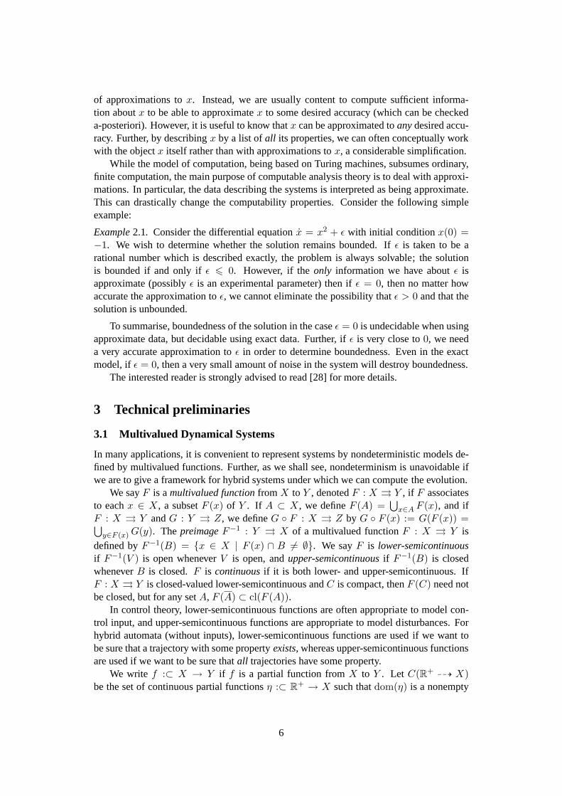
activated when the constraintc1 given byx > a. The solution to the continuous dynamicsin modeq1 is (x(t), y(t)) = (x0 + 2y0t− t2, y0 − t). The maximum value ofx is x0 + y2

0

and is attained whent = y0.

X1

X2

Figure 4: A hybrid automaton with two discrete modes and piecewise-affine dynamics ex-hibiting a grazing discontinuity.

Suppose the initial condition is(q1, x0, y0) with x0 = −1 andy0 = +1. Thenx(t)reaches a maximum value of0 at t = 1. Consider the setΨH((x0, y0), t = 2). Then ifa > 0, the constraintc1 is not satisfied, and the reached state is(q1,−1,−1). However,if a < 0, the constraintc1 is satisfied for somet < 1, and the state at timet = 2 is (q2).Hence the evolution is discontinuous in the parametera.

Now suppose thata is fixed at0, and the initial condition is(x0, 1) with x0 < 0. Thenfor x0 < −1, the maximum value ofx is 1 + x0 which is less thana, so the constraint isnever active and the reached state is(q1, x0,−1). However, ifx0 > −1, the constraintc1 issatisfied for somet < 1 and the reached state is(q2). Hence the evolution is discontinuousin the parametera.

Example4.4 (Discontinuity induced by corner collisions). Let H be a hybrid automatonwith three modesq1, q2 andq3, with X1 = R2 andX2 = X3 = R0. The dynamics inX1

has constant derivative,(x, y) = (1, 1). There are two events,e2 ande3, with reset maps,r2 andr3 with r2(q1, x, y) = (q2) andr3(x, y) = (q3), and activationsc2 which is activatedwhenx > a, andc3 which is activated wheny > b.

X1 X3

X2

Figure 5: A hybrid automaton with three discrete modes, affine guard sets and piecewise-constant dynamics exhibiting a corner discontinuity.

Suppose the initial condition is(q1, x0, y0) with x0 = y0 = 0. Then if0 < a < b < 1,the evente2 is activated beforee3, and the state at timet = 1 is (q2). If 0 < b < a < 1,then evente3 is activated beforee2, and the state at timet = 1 is (q3). Hence the evolutionis discontinuous in the parametersa andb. In a similar way, we can show that the evolutionis discontinuous in the initial state.

Example4.5 (Discontinuity induced by immediately activated events). Let H be a hybridautomaton with three modesq1, q2 andq3, with X1 = R2, X2 = R andX3 = R0. Thedynamics inX1 has constant derivative,(x, y) = (1, 0), and the dynamics inX2 is x = 1.

12

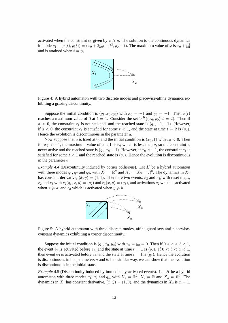
The evente1 is may occur in modeq1, with activationx > a and resetr1(q1, x, y) = (q2, x+y). The evente2 may occur in modeq2, with activationx 6 0 and resetr2(q2, z) = (q3).

X1

X2

X3

Figure 6: A hybrid automaton with three discrete modes, affine guard sets and piecewise-constant dynamics exhibiting a discontinuity caused by an immediately activated event.

Suppose the initial condition is(q1, x0, y0) with x0 = −1 andy0 = 0. Then the evente1 is activated at(q1, a, 0) and the state is reset to(q2, a). If a < 0, evente2 is immediatelyactivated, and a transition occurs to state(q3). If a > 0, then the continuous statez in modeq2 satisfiesz > a > 0, and so evente2 is never activated, and the state at timet for t > 1 is(q2, t− 1). Hence the evolution is discontinuous in the parameters.

If the initial state is(q1,−1, y0), then the evente1 is activated at(q1, a, y0) and the stateis reset to(q2, z) with z = a + y0. If y0 > −a, the state remains in modeq2 whereas ify0 < −a, thenz < 0 and evente2 is immediately activated and the state is reset to(q3).Hence the evolution is discontinuous in the initial state.

4.4 Coherent semantics of evolution

We have seen that the evolution operatorΨ : X×R+ → X of a non-Zeno hybrid automatonmay be discontinuous in both space and time, even for affine systems. By the fundamentaltheorem of computable analysis, this means that the evolution is uncomputable, at leastnear the discontinuity points. This does not in itself rule out the possibility of regularisingthe evolution in some way so that the evolution becomes computable. In Section 5 weshall show that by using appropriately-defined nondeterministic semantics,we can makethe evolution semicomputable. In this subsection we prove that it is impossible to regularisethe evolution near continuity points to make the solution fully computable i.e. both lower-and upper-semicomputable.

Definition 4.6 (Coherent semantics of evolution). Let H = (X,R,Φ) be a hybrid au-tomaton, and letU ⊂ X × R+ be the domain of continuity of the solution operatorΨ : X × R+ → X. We say that a set-valued solution operatorΨ : X × R+ ⇉ Xhascoherent semanticsif Ψ(x, t) = {Ψ(x, t)} for all (x, t) ∈ U .

In other words, away from discontinuities, the solution operatorΨ must be single-valued, with the value given byΨ. This condition eliminates trivial approximations, such astakingΨ(x, t) = X for all x ∈ X, t ∈ R+. For maximum flexibility, we give no restrictionson the discontinuity set.

Theorem 4.7(Uncomputability of the evolution of hybrid automata). LetH be a class ofhybrid automata. Then for any coherent semantics of evolution, the finite-time evolution ofa hybrid system is uncomputable. This result holds even if we restrict to(x, t)-values forwhich no event occurs at timet.

In particular, the operator(X0, t) 7→ ΨH(X0, t) is not (κ, ρ;κ)-computable. Further,even if no event is possible at timet, the operatorx 7→ ΨH(x, t) is not(κ;κ)-computable.

13

The result is immediate from the following general lemma, since we have seen examplesfor which the evolution has non-removable discontinuities, even away fromdiscrete events.

Lemma 4.8. Let f : U → Y be single-valued and continuous on an open, dense subsetUofX, and letY be compact. Supposef has no continuous closed-valued extension overX.Thenf has no continuous multivalued extensionF overX.

Proof. For letx be an essential discontinuity point off , andA =⋂

x∈V cl(f(V ∩U)) overopen setsV . SupposeF (x) ⊂6= A, let y ∈ A \ F (x), and take a closed neighbourhoodBof y such thatA ∩B = ∅. ThenF−1(B) does not containx, but contains points arbitrarilyclose tox, soF would not be upper-semicontinuous. SupposeF (x) ⊃ A andA has twodistinct elementsy andz. LetW be an open neighbourhood ofy such thatcl(W ) is disjointfrom z. ThenF−1(W ) containsx but does not contain points inF−1(X \ cl(W )) whichcome arbitrarily close tox, soF is not lower-semicontinuous.

4.5 Sliding along switching boundaries

A particularly nasty form of discontinuity occurs when a solution slides alongthe boundaryof a guard set before crossing.

Example4.9 (Uncomputability caused by sliding). Consider a hybrid automaton in two-dimensions with a transition which is active fory > 0. Consider the flowx = 1, and

y =

a+ 3x2 − y if x 6 0;

a− y if 0 6 x 6 b;

a+ 3(x− b)2 − y if x > b

.

Fora = 0, and let(x0, y0) be a point withx0 < 0 such that the continuous orbit starting at(x0, y0) exactly reaches the point(0, 0). Then forb > 0, the continuous evolution startingat (x0, y0) slides along the surfacey = 0 for 0 6 x 6 b, and then crosses intoy > 0. Thehybrid orbit therefore undergoes a discrete transition at some point(x, 0) with 0 6 x 6 b,but the exact value ofx at which this transition occurs is undetermined. Fora > 0, we seethaty > 0 wheny = 0, and the orbit starting at(x0, y0) undergoes a discrete transition withx < 0, whereas fora < 0, the orbit starting at(x0, y0) undergoes a discrete transition withx > b. Hence the spacial evolution is discontinuous at the parameter valuea = 0. Since fora lower-approximation to the solution we may only consider solutions which persist underperturbations, the hybrid evolution starting at(x0, y0) cannot be continued past the point(0, 0).

Now consider the casea = 0 and b = 0, which is the limit of the casesa = 0,b > 0. Since the hybrid orbit starting at(x0, y0) is blocked at(0, 0) for b > 0, in the limitb = 0, the orbit cannot be continued past(0, 0) when computing lower-approximations.However, the dynamics in this case is given by the differential equation(x, y) = (1, 3x2 −y), so all solutions which reachy = 0 cross topologically transversely. This implies thattopological transversality of crossing a guard set is not in itself sufficient to ensure that adiscrete transition is enabled at the crossing point.

Now consider the flow(x, y) = (1, 0) the guard setx = y and reset map(x, y, q0) 7→(y, q1). The flow is transverse to the guard set, and if the initial state if(x, c, q0) withx < y, then after the first reset the new state is(c, q1). However, it is possible to makeaC0 perturbation of the guard set, so that the flow is parallel to the guard set for y = a.By the previous discussion, this means that the evolution of the perturbed hybrid system

14

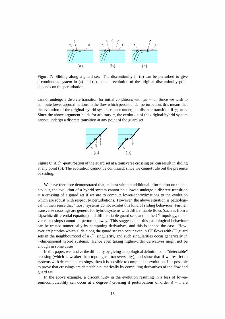
(b)(a) (c)

Figure 7: Sliding along a guard set. The discontinuity in (b) can be perturbed to givea continuous system in (a) and (c), but the evolution of the original discontinuity pointdepends on the perturbation.

cannot undergo a discrete transition for initial conditions withy0 = a. Since we wish tocompute lower approximations to the flow which persist under perturbation, this means thatthe evolution of the original hybrid system cannot undergo a discrete transition if y0 = a.Since the above argument holds for arbitrarya, the evolution of the original hybrid systemcannot undergo a discrete transition at any point of the guard set.

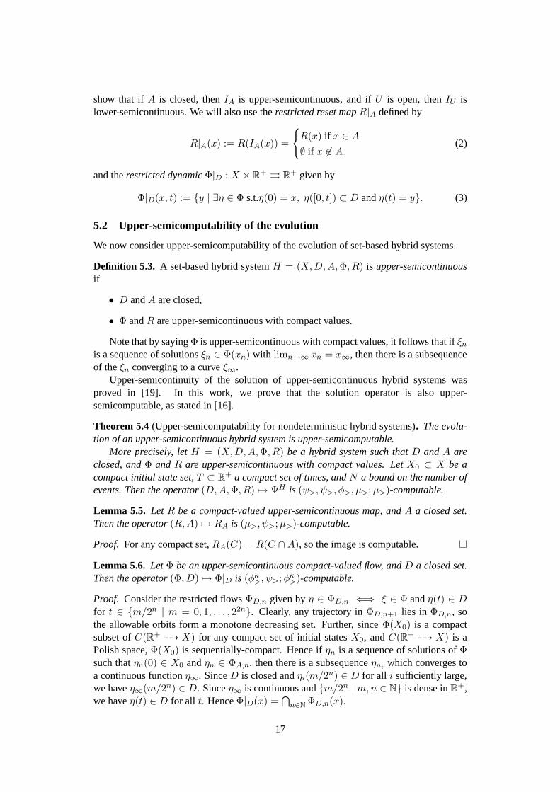
(a) (b)

Figure 8: AC0-perturbation of the guard set at a transverse crossing (a) can result in slidingat any point (b). The evoluition cannot be continued, since we cannot rule out the presenceof sliding.

We have therefore demonstrated that, at least without additional informationon the be-haviour, the evolution of a hybrid system cannot be allowed undergo a discrete transitionat a crossing of a guard set if we are to compute lower-approximations to theevolutionwhich are robust with respect to perturbations. However, the above situation is pathologi-cal, in then sense that “most” systems do not exhibit this kind of sliding behaviour. Further,transverse crossings are generic for hybrid systems with differentiableflows (such as from aLipschitz differential equation) and differentiable guard sets, and in theC1 topology, trans-verse crossings cannot be perturbed away. This suggests that this pathological behaviourcan be treated numerically by computing derivatives, and this is indeed the case. How-ever, trajectories which slide along the guard set can occur even inCr flows withCr guardsets in the neighbourhood of aCr singularity, and such singularities occur generically inr-dimensional hybrid systems. Hence even taking higher-order derivatives might not beenough in some cases.

In this paper, we resolve the difficulty by giving a topological definition of a“detectable”crossing (which is weaker than topological transversality), and show that if we restrict tosystems with detectable crossings, then it is possible to compute the evolution. Itis possibleto prove that crossings are detectable numerically by computing derivatives of the flow andguard set.

In the above example, a discontinuity in the evolution resulting in a loss of lower-semicomputability can occur at a degree-d crossing if perturbations of orderd − 1 are

15

allowed. Hence, a purely topological approach to lower-approximations insystems withcrossings of guard sets is bound to fail.

5 Semicontinuity of evolution of hybrid systems

We now introduce a class of nondeterministic hybrid systems and consider conditions underwhich the evolution is semicomputable.

5.1 Nondeterministic hybrid systems

In this paper, we use the following definition of hybrid system, which slightly extends thatof [4], and is essentially equivalent to that used in [19].

Definition 5.1 (Hybrid system). A hybrid systemis a tupleH = (X,D,A,Φ, R) where

• the state spaceX is a manifold,

• D ⊂ X is thedomainset,

• A ⊂ X is theactivationset.

• Φ : X ⇉ C(R+ 99KX) is a multivaluedflow, and

• R : X ⇉ X defines aresetmapx′ ∈ R(x).

In typical examples, the flow will be defined by a differential equationx = f(x) or differ-ential inclusionx ∈ F (x).

Note that instead of working with differential inclusions, we work directly withflows,since this separates the core hybrid systems theory (e.g. detecting crossings with guardsets) from the technicalities of integrating with differential inclusions. IfA andD form atopological partition ofX (i.e.D ∪A = X andD◦ ∩A◦ = ∅, where◦ denotes the interiorof a set), andΦ is given by the differential inclusionx ∈ F (x) thenH = (X,A, F,R) isan impulse differential inclusionas defined in [4].

Definition 5.2 (Trajectories of hybrid systems). A trajectory or solution of a hybrid systemH = (X,D,A,Φ, R) is a hybrid trajectoryξ : T → X such that

• ξ(t, n) ∈ D whenevertn 6 t 6 tn+1,

• ξ(tn, n− 1) ∈ A,

• ξ(t, n) = η|[0,tn+1−tn](t− tn) for someη ∈ Φ, and

• ξ(tn, n) ∈ R(ξ(tn, n− 1)).

Note that even ifΦ andR are single-valued, then the evolution can still be nondeter-ministic. For if x ∈ D ∩ A, then both continuous evolution and a discrete jump may bepossible starting fromx.

In this section, we will make regular use of the set-valued indicator functionIS : X ⇉X defined byIS(x) = {x} if x ∈ S, andIS(x) = ∅ if x 6∈ S. It is straightforward to

16

show that ifA is closed, thenIA is upper-semicontinuous, and ifU is open, thenIU islower-semicontinuous. We will also use therestricted reset mapR|A defined by

R|A(x) := R(IA(x)) =

{R(x) if x ∈ A

∅ if x 6∈ A.(2)

and therestricted dynamicΦ|D : X × R+ ⇉ R+ given by

Φ|D(x, t) := {y | ∃η ∈ Φ s.t.η(0) = x, η([0, t]) ⊂ D andη(t) = y}. (3)

5.2 Upper-semicomputability of the evolution

We now consider upper-semicomputability of the evolution of set-based hybrid systems.

Definition 5.3. A set-based hybrid systemH = (X,D,A,Φ, R) is upper-semicontinuousif

• D andA are closed,

• Φ andR are upper-semicontinuous with compact values.

Note that by sayingΦ is upper-semicontinuous with compact values, it follows that ifξnis a sequence of solutionsξn ∈ Φ(xn) with limn→∞ xn = x∞, then there is a subsequenceof theξn converging to a curveξ∞.

Upper-semicontinuity of the solution of upper-semicontinuous hybrid systemswasproved in [19]. In this work, we prove that the solution operator is also upper-semicomputable, as stated in [16].

Theorem 5.4(Upper-semicomputability for nondeterministic hybrid systems). The evolu-tion of an upper-semicontinuous hybrid system is upper-semicomputable.

More precisely, letH = (X,D,A,Φ, R) be a hybrid system such thatD andA areclosed, andΦ andR are upper-semicontinuous with compact values. LetX0 ⊂ X be acompact initial state set,T ⊂ R+ a compact set of times, andN a bound on the number ofevents. Then the operator(D,A,Φ, R) 7→ ΨH is (ψ>, ψ>, φ>, µ>;µ>)-computable.

Lemma 5.5. LetR be a compact-valued upper-semicontinuous map, andA a closed set.Then the operator(R,A) 7→ RA is (µ>, ψ>;µ>)-computable.

Proof. For any compact set,RA(C) = R(C ∩A), so the image is computable.

Lemma 5.6. Let Φ be an upper-semicontinuous compact-valued flow, andD a closed set.Then the operator(Φ, D) 7→ Φ|D is (φκ

>, ψ>;φκ>)-computable.

Proof. Consider the restricted flowsΦD,n given byη ∈ ΦD,n ⇐⇒ ξ ∈ Φ andη(t) ∈ Dfor t ∈ {m/2n | m = 0, 1, . . . , 22n}. Clearly, any trajectory inΦD,n+1 lies in ΦD,n, sothe allowable orbits form a monotone decreasing set. Further, sinceΦ(X0) is a compactsubset ofC(R+ 99K X) for any compact set of initial statesX0, andC(R+ 99K X) is aPolish space,Φ(X0) is sequentially-compact. Hence ifηn is a sequence of solutions ofΦsuch thatηn(0) ∈ X0 andηn ∈ ΦA,n, then there is a subsequenceηni

which converges toa continuous functionη∞. SinceD is closed andηi(m/2

n) ∈ D for all i sufficiently large,we haveη∞(m/2n) ∈ D. Sinceη∞ is continuous and{m/2n | m,n ∈ N} is dense inR+,we haveη(t) ∈ D for all t. HenceΦ|D(x) =

⋂n∈N ΦD,n(x).

17

It remains to show that eachΦD,n is computable. It is sufficient to consider{η | ξ(t) ∈D} is a computable closed set inD for all t ∈ R+, since then we can writeΦD,n(x0) =

Φ(x0) ∩⋂22n

m=0{ξ | η(m/2n) ∈ D}. This follows since

{η | η(t) 6∈ D} =⋃

{(T,J)∈βR×βX |J∩D 6=∅ andt∈T}{η | η(T ) ⊂ J}

and{η ∈ Φ | η(T ) ⊂ J} = cl({η ∈ Φ | η(T ) ⊂ J})

Hence{η | η(t) ∈ D} is the complement of⋃

(J,T )|J∩D 6=∅ andt∈T cl({)η | η(T ) ⊂ J},which can be computed fromD.

We can now give the proof of Theorem 5.4.

Proof. By Lemmas 5.5 and 5.6, we can obtain aµ>-name of the restricted resetR|A and aφ>-name of the restricted flowΦ|D. It remains to compute aµ>-name of the evolutionΨ.

Consider the caseD = A = X, soΦ|D = Φ andRA = R. Let Ψh(x) := Φ|D(x, t).Then we can obtain aµ> name of(x, t) 7→ Φ(x, t). Define

Ψ(x, t; t1, . . . , tn) = {y ∈ X | ∃ solutionξ of H with event timest1 6 · · · 6 tn 6 t

s.t. ξ(0, 0) = x andξ(t, n) = y}.

Then since we can write

Ψ(x, t, (t1, . . . , tn)) = Φt−tn ◦R ◦ Φtn−tn−1◦ · · · ◦R ◦ Φt1(x)

we see that the map(x, t, t1, . . . , tn) 7→ Ψ(x, t, (t1, . . . , tn)) is a composition of functionsfor which we haveµ>-names, and hence we can computeµ>-name ofΨ. We can writeΨ(x, t, n) = Ψ(x, t, Tt,n) whereTt,n = {(t1, . . . , tn) ∈ Rn | ∀i, 0 6 ti 6 ti+1 6t}. Sincet 7→ Tt,n is (ρ, κ>)-computable, we can compute aµ>-name of the function(x, t, n) 7→ Ψ(x, t, n). ThenΨ(x, t, [0, N ]) =

⋃∞n=0 Ψ(x, t, n) =

⋃Nn=0 Ψ(x, t, n) is a

finite union ofµ>-computable functions. Hence we can compute aµ>-name ofΨ.

We say a system isuniformly non-Zenoif there exist(T,N) such that in any timeinterval of length at mostT , there occur at mostN discrete events. As shown in [19],any non-Zeno upper-semicontinuous hybrid system with a compact globalattractor mushbe uniformly non-Zeno. For non-Zeno systems, we can drop the bounds on the number ofevents.

Corollary 5.7 (Upper-semicomputability for non-Zeno hybrid systems). Let H =(X,D,A,Φ, R) be a uniformly non-Zeno upper-semicontinuous hybrid system LetX0 ⊂ Xbe a compact initial state set, andT ⊂ R+ a compact set of times. Then the operator(D,A,Φ, R,X0, T ) 7→ ΨH(X0, T ) is (ψ>, ψ>, φ>, µ>;µ>)-computable.

5.3 Lower-semicomputability of evolution

Definition 5.8. A hybrid systemH = (X,D,A,Φ, R) is lower-semicontinuousif

• D andA are open, and

• Φ andR are lower-semicontinuous with closed values.

18

In this situation, we have the following computability result.

Theorem 5.9.The evolution of a lower-semicontinuous domain-activation hybrid system islower-semicomputable.

More precisely, letH = (X,D,A,Φ, R) be a hybrid system, whereD andA are open,Φ is a lower-semicontinuous multivalued flow, andR : X ⇉ X is lower-semicontinuous.LetX0 ⊂ X be closed andT ⊂ R+ be closed. Then the operator(D,A,Φ, R) 7→ clΨH

is (θ<, θ<, θ<, µ<;µ<)-computable. Equivalently, the operator(D,A,Φ, R,X0, T ) 7→clΨH(X0, T ) is (θ<, θ<, θ<, µ<, ψ<, ψ<;ψ<)-computable

The basic idea of the proof is as follows. We leth be a time step, and consider alltrajectories ofH such that discrete events are constrained to occur at timeskh with 0 <kh < t. We show that the evolution defined by this semantics is lower-semicomputable,and that in the limit ash → ∞ we obtain all trajectories. It is important that we do notallow a discrete transition to occur at the initial or final time of the evolution.

Lemma 5.10. Let R be a closed-valued lower-semicontinuous map, andU an open set.Then the operator(R,U) 7→ R|U is (µ<, θ<;µ<)-computable.

Proof. From the definition ofIU , we haveJ ⊂ I−1U (K) iff J ⊂ U ∩ K so the function

U 7→ IU is (θ<;µ<)-computable. The result follows sinceRU = R ◦ IU = cl(R ◦ IU ), andcomposition of functions is a lower-semicomputable operation.

Lemma 5.11. Let Φ be an lower-semicontinuous closed-valued flow, andD an open set.Then the operator(Φ, D) 7→ Φ|D is (φA<, θ<;φA<)-computable.

Proof. We first show that for allt > 0, {η | η([0, t]) ⊂ D} is computable. We see that forfixed η andt ∈ Q thatη([0, t]) ⊂ D ⇐⇒ ∃0 = t0 < t1 < · · · < tk = t, J1, . . . , Jk withJ i ⊂ D such thatη([ti−1, ti]) ⊂ Ji. so we can write

{η | η([0, t]) ⊂ D

}=

⋃{(ti,Ji)∈(Q×β)∗|Ji⊂D}

⋂{η | η([ti−1, ti]) ⊂ Ji}

which is a computable (from aθ<-name ofD) countable union of finite intersections ofbasic open sets.

HenceΦ|D is the closure of the intersection ofΦ with the union of partial trajectoriessuch thatη([0, tn]) ⊂ D, so is computable.

We now present the proof of Theorem 5.9

Proof. First consider the caseD = A = X, so thatΦ = Φ|D andR = R|A. Notethat from aφ<-name ofΦ as a mapX ⇉ C(R+ 99K X), we can compute aµ<-nameof Φ as a mapX × T ⇉ X. DefineΨ(x, t; t1, . . . , tn) andTt,n as in the proof of The-orem 5.4. Then the mapt 7→ Tt,n is lower-semicomputable i.e.(ρ;ψ<)-computable, andsince(x, t, t1, . . . , tn) 7→ Ψ(x, t; t1, . . . , tn) is a composition of maps of the formΦti−ti−1

andR, for which we haveµ<-names, we can compute aµ<-name oft 7→ Ψ(x, t). Hencewe can compute aµ<-name of the closed composition(x, t) 7→ cl(Ψ(x, t)).

The general case follows from the fact that(D,Φ) 7→ Φ|D and (A,R) 7→ R|Aare lower-semicomputable i.e. respectively(θ<, φ<;φ<)-computable and(θ<, µ<;µ <)-computable.

19

The following result will be useful in Section 5.6. It shows that the evolutionofH is thesame as the evolution we obtain by considering only trajectories with distinct event times.Indeed, any solution ofH is the limit of solutions with distinct event times. Formally, letHbe a hybrid system and defineΨ by

Ψ(x, t, n) = {y | ∃ solutionξ of H with event times0 < t1 < t2 < · · · < tn < t

such thatξ(0) = x andξ(t) = y}. (4)

Proposition 5.12. Let Ψ be the evolution of a lower-semicontinuous hybrid systemH,and letΨ be the evolution ofH consisting of trajectories with distinct event times. Thencl(Ψ(x, t)) = cl(Ψ)(x, t).

Proof. Define Ut,n = {(t1, . . . , tn) ∈ Rn | 0 < t1 < · · · < tn < t}. ThenΨ(x, t) = Ψ(x, t, Ut,n) whereΨ(x, t, (t1, . . . , tn)) is as defined previously. SinceΨ : X ×

R+ × (R+)n ⇉ X is lower-semicontinuous, we havecl(Ψ(x, t, n)) = cl(Ψ(x, t, Ut,n)) =cl(Ψ(x, t, U t,n)) = cl(Ψ(x, t, Tt,n)) = cl(Ψ(x, t, n)) as required.

5.4 Closure and interior semantics of evolution

General hybrid systems of the form given by Definition 5.1 need not be upper- or lower-semicontinuous. In order to compute upper- or lower approximations to the solution, weneed to convert the system into either upper- or lower-semicontinuous form. We can do thisbe regularising the guard sets to be open or closed, and

Definition 5.13. LetF : X ⇉ Y be a multivalued function. Define

• F by F =⋃{F | F is upper-semicontinuous andF ⊂ F}, and

• F by F =⋃{F | F is lower-semicontinuous andF ⊂ F}.

An alternative definition ofF is in terms of its graph;Graph(F ) =⋂

ǫ>0Nǫ(GraphF ).It is easy to show that ifF locally takes pre-compact values (i.e.cl(F (I)) is compact for anycompactI) thenF is compact-valued upper-semicontinuous, and thatF is closed-valuedlower-semicontinuous.

Definition 5.14. LetH = (X,D,A, F,R) be a set-based hybrid system. Then

• ξ : T → X is a trajectory ofH usingclosure-semanticsif ξ is a trajectory of theupper-semicontinuous systemH = (X, cl(D), cl(A),Φ, R).

• ξ : T → X is a trajectory ofH using interior-semanticsif ξ is a trajectory of thelower-semicontinuous systemH = (X,D◦, A◦,Φ, R).

From Theorems 5.4 and 5.9, we deduce

Corollary 5.15. LetH = (X,D,A, F,R) be a set-based hybrid system. Then the evolutionofH is upper-semicomputable and the evolution ofH is lower-semicomputable.

We now show thatH is “smallest” hybrid system for which the evolution is upper-semicomputable. In other words,any attempt to compute an over-approximation to theevolved set using approximative methods must necessarily compute an over-approximateionto the evolved set ofH.

20

We letH be the space of hybrid systems, whereD andA are in the space of regularsets with both the lower representationθ< and upper representationψ>, Φ is in the space ofcompact-valued flows with representationφ = φ< ∨ φ>, andR is in the space of compact-valued maps with representationµ< ∨ µ>. In other words,D is a regular set, and we haveaccess to a list of boxes fillingD◦, and a list of boxes fillingX \ cl(D).

Theorem 5.16. LetH = (X,D,A,Φ, R) be a hybrid system, and suppose thatΨ : H ×X × R 7→ K(X) is upper-semicomputable andΨ(x, t) ⊃ ΨH(x, t) for all x, t. ThenΨ(x, t) ⊃ ΨH(x, t).

We have a similar result for lower-semicontinuity.

Theorem 5.17. Let H = (X,D,A,Φ, R) be a hybrid system, and suppose thatΨ :XH× R 7→ A(X) is lower-semicomputable andΨ(x, t) ⊂ cl(ΨH(x, t)) for all x, t. ThenΨ(x, t) ⊂ cl(ΨH(x, t)).

The significance of these results is that, in general, it is impossible to do better thancompute over- or lower- approximations to the evolution which converge to smaller setsthan those given by the upper or lower semantics, as long as only approximate informationis used.

5.5 Deficiencies of interior semantics

Unfortunately, the definition of interior-semantics given causes difficultiesin the modellingof systems with urgent transitions. This is because there is no way in the formalism ofspecifying a coupling between the invariants and activations.

Example5.18 (Uncomputability caused aliasing). Consider a system with dynamicx = 1,invariant x 6 a and activationx > b with a, b > 0. If a < b, then the invariant isviolated before the transition is activated, and further evolution is blocked.If a > b, thenthe transition is activated before the invariant is violated, and a transition may occur at anytime b < x(t) < a. If a = b and we are computing an over-approximation to the evolution,then a transition must occur exactly whenx(t) = a. However, if we are computing a lower-approximation to the evolution, then since equality is undecidable, we need to consider thepossibility thata < b. Hence a lower-approximation to the evolution must block, since thisis the worst-case scenario.

(b)(a) (c)

Figure 9: Discrete transitions are blocked using inner semantics even at a transverse cross-ing. In (a) the domain and activation regions overlap and crossings are possible. In (b) theboundaries of the domain and activation regions touch, and discrete transitions are forcedwith upper semantics, but disallowed using inner semantics. An arbitrarily smallperturba-tion gives (c) in which no transitions are possible.

At first sight, it may seem that the evolution “should” continue fora = b. However,the correct semantics for lower-approximation is to block the evolution. This isbecause

21

if the invariant and activation are determined by independent parameters,then it is onlya coincidence that the transition is activated at exactly the same point as the invariant isviolated, and under a small change in the parameters then the evolution may be blocked. Itis only if we give the additional, combinatorial information that the invariant andactivationboundaries lie exactly at the same point, that we can deduce that the evolutionmay continue.From an implementation standpoint, we see thatx 6 a andx > b are aliases for the sameconstraintx ⋚ c with c = a = b.

5.6 Lower-semicomputability of hybrid systems using crossing semantics

Let H = (X,D,A,Φ, R) be a hybrid system and supposeD andA are regular open setsandΦ is closed-valued lower-semicontinuous. We would like to know when trajectories ofH cross instantaneously fromD toA.

Definition 5.19. A continuous trajectoryξ crosses fromD toA at timet and pointx if forall δ > 0, ξ(t− δ, t)∩D 6= ∅ andξ(t, t+ δ)∩A 6= ∅. We say thatx is acrossing pointforξ.

Note that trivially ifx ∈ D ∩ A, thenx is a crossing point for any trajectory though it.If x 6∈ cl(D) ∩ cl(A), thenx cannot be a crossing point. The real interest is whenx lies in∂D and∂A. By the observations of Example 5.18, ifD andA are disjoint, then by a smallperturbation, we can make their boundaries disjoint, and so any lower approximation to theflow will have blocking. We therefore need more information about the setsD andA, andthe flowΦ than is given by the namesθ< andφ<.

Let us consider the case in whichD andA form a topological partition ofX; that is,D ∩ A = ∅ andcl(D) ∪ cl(A) = X. Supposeξ is a trajectory such thatξ(t1) ∈ D andξ(t2) ∈ A, soξ apparently crosses fromD to A. We would like to be able to deduce thatξ crosses fromD toA in the sense of Definition 5.19. Unfortunately, from Example 4.9, itmay be the case thatξ slides inside∂D ∩ ∂A rather than crossing transversely, and as wehave seen, we cannot handle sliding solutions.

Definition 5.20. LetH be a hybrid system andδ > 0. We sayH hasδ-detectable crossingsif for all trajectoriesξ of Φ such thatξ(0) ∈ D andξ(t) ∈ A for somet < δ, then thereexistsc ∈ R andη ∈ Φ such thatξ([0, c[) ⊂ D, η(0) = ξ(c) andη([0, ǫ[) ∩ A 6= ∅ for allǫ > 0.

In other words, if there is a trajectory which moves fromD to A in time less thanδ, then from the point where the state leavesD, there is a possibly different trajectoryηwhich immediately entersA. Note that the condition of detectable crossings precludes thedegenerate situation in which a solution slides along a common boundary ofD andA fortime less thanδ, and also the case of Example 5.18 in which the solution leavesD brieflybefore enteringA.

In Section 6.3, we will give conditions under which a system has detectable crossings.We now define a new notion of solution for hybrid systems.

Definition 5.21. Let H = (X,D,A,Φ, R) be a hybrid system whereD andA are opensets. Then a hybrid trajectoryξ is a solution ofH usingcrossing semanticsif

• 0 < t1 < t2 < · · · < ti < ti+1 < · · · .

• ξ[t, n) ∈ D for tn 6 t < tn+1.

22

• There existsζn ∈ Φ such thatζn(0) = ξ(tn, n) andζn([0, ǫ[) ∩A 6= ∅ for all ǫ > 0.

• ξ(·, n) ∈ Φ, and

• ξ(tn, n) ∈ R(ξ(tn, n− 1)).

Intuitively, between discrete events, solutions must remain in the interior ofD; thisprevents grazing contact with guard sets. A discrete event may occur atthe boundary ofDif it is possible to continue the trajectory directly intoA. Note that after a reset, we requireeither thatx ∈ D or that another discrete transition occurs immediately. Note that we allowξ(tn, n) 6∈ D if another event occurs exactly at timetn.

Using this notion of solution, we can prove the following result.

Theorem 5.22(Lower-semicomputability of the evolution of hybrid systems with detectiblecrossings). Let H be a lower-semicontinuous hybrid system withδ-detectable crossings.Then the evolutionH 7→ ΨH(x, t) is lower-semicomputable using crossing semantics.

More precisely, letH = (X,D,A,Φ, R) be a hybrid system whereD andA are opensets, andΦ andR are lower-semicontinuous with closed values. Suppose that crossings ofΦ fromD to A are δ-detectable. LetX0 be a closed set of initial states, andT is an openset of times. The the operator(D,A,Φ, R) 7→ ΨH is (θ<, θ<, φ<, µ<;µ<, )-computable.

We use the following lemma, which shows that the crossing times and points can becomputed.

Lemma 5.23. LetD andA be open sets andΦ be a lower-semicontinuous closed-valuedflow. Suppose that the crossings of trajectories ofΦ fromD to A are δ-detectable. Definethe crossing functionΓ : X ⇉ R+ ×X by

Γ(x0) = {(t, x) ∈ R ×X | t > 0 and∃ξ ∈ Φ s.t. ξ([0, t)) ⊂ D and

ξ([0, t+ ǫ[) ∩A 6= ∅ for all ǫ > 0}. (5)

Then the function(D,A,Φ) 7→ Γ is (θ<, θ<, φ<;µ<)-computable.

Proof. Consider the set of trajectories ofΦ which have a first crossing fromD toA at timet ∈]t1, t2[ and pointx ∈ J , and supposet1 < t2 < t1 + δ. If η is such a trajectory, then bythe definition of crossing, we haveη([0, t1]) ⊂ D, η([t1, t2]) ⊂ J andη([t1, t2]) ∩ A 6= ∅.Further, by theδ-detectable crossing condition, this is a sufficient condition for the existenceof a crossing at timet ∈]t1, t2[ and pointx ∈ J . HenceI ⊂ Γ−1(T × J) if and only if

I ⊂ Φ−1({η | η([0, t1]) ⊂ D} ∩ {η | η([t1, t2]) ⊂ J} ∩ {η | η([t1, t2]) ∩A 6= ∅}

)

The set{η | η([0, t1]) ⊂ D} can be lower-semicomputed from aθ< name ofD, and the set{η | η([t1, t2]) ⊂ J} is a basic open set of the flow. The set{η | η([t1, t2]) ∩ A 6= ∅} canbe written as

⋃T⊂[t1,t2]{η | η(T ) ⊂ A}, so is a countable union of lower-semicomputable

sets. Hence we can enumerate all tuples(I, T, J) ∈ βX × βR × βX such that for allx ∈ I,there exists a trajectory ofΦ starting atx such thatΦ has a first crossing fromD to A attime t ∈ T and pointy ∈ J , which means we have aµ<-name ofΓ.

We can now give the proof of Theorem 5.22

23

Proof. DefineΨ : X × R+ × N+ ⇉ X to be the evolution ofH with crossing semantics.Note that this means that all events must occur at distinct times. DefineR : X×R ⇉ X×R

by R(x, t) = R(x) × {t}, andΘ((x, s), t) = Φ(x, t − s) for x ∈ X and0 < s < t. ThenΨ(x, t, 1) = Θ(R(Γ(x)), t). It is clear that we can compute aµ<-name ofR andΘ fromµ<-names ofR andΦ, respectively, and by Lemma 5.23 we can compute aµ<-name ofΓ. Hence we can compute aµ< name of the composition(x, t) 7→ cl(Ψ(x, t, 1)). Theresult by induction sinceΨ(x, t, n+ 1) =

⋃s∈]0,t[ Ψ(Ψ(x, s, b), t− s, 1) andcl(Ψ(x, t)) =

⋃∞n=0 Ψ(x, t, n)

Note that in the case of crossing semantics, it is not true that every trajectory withmultiple events at the same time is a limit of trajectories with distinct event times.

6 Modelling, Simulation and Implementation

6.1 Hybrid Automata with guard sets

The description of hybrid automata introduced in Section 4 is sufficient to define the dy-namic evolution, but is inexpressive as a modelling framework. Many hybridsystem modelsare defined using explicitdiscrete state, anddiscrete eventsand allow forurgent transitionswhen a trajectory first touches aguard set. Guard sets therefore form both the boundaryof the invariant domain of continuous evolution, and of the activation regionof the discreteevent. We should therefore use crossing semantics for determining the activation of eventsgiven by guard sets when computing lower-approximations to the evolution. We can useinterior semantics when determining the activation of non-urgent orpermissivetransitions.

In our definition of hybrid systems we will describe sets in terms ofconstraint functions.A constraint is a continuous functionc : X → R, and we say a constraint isregular if{x ∈ X | c(x) = 0} is a codimension-1 topological manifold. Ifc is differentiable and∇c(x) 6= 0 wheneverc(x) = 0, thenc is regular, and changes sign on a differentiablemanifold.

A constraint defines sets{x ∈ X | c(x) ≶ 0} and{x ∈ X | c(x) ⋚ 0}. The operatorc 7→ {x | c(x) < 0} is (γ; θ<)-computable and the operatorc 7→ {x | c(x) 6 0} is(γ;ψ <)-computable.

We now give a standard definition of hybrid automata. A transition for a constrainthybrid automaton is eitherurgent(sometimes calledjust-in-time), which means that contin-uous evolution is not allowed when the event is active, ornon-blocking, which means thatcontinuous evolution is allowed in addition to a discrete transition, and hence thedynamicsis nondeterministic.

Definition 6.1 (Hybrid automaton). A constraint hybrid systemis a tupleH = (Q,E =EU ∪ EP , γ, {Xq | q ∈ Q}, {Fq | q ∈ Q}, {Dq | q ∈ Q}, {(Rq,e | (q, e) ∈dom γ}, {(Aq,e | (q, e) ∈ dom γ, e ∈ EP }, {(gq,e | (q, e) ∈ dom γ, e ∈ EU})) where

• Q is a finite set ofdiscrete statesandE is a finite set ofdiscrete events, which ispartitioned into subsetsEU of urgent eventsandEP of permissive events.

• γ :⊂ Q× E → Q is a partialdiscrete transition functionwith domaindom γ.

• For eachq, the manifoldXq is thecontinuous state spacefor discrete stateq.

24

• For eachq, Fq : Xq ⇉ TXq is a differential inclusion giving thecontinuous dynam-ics.

• For eachq,Dq ⊂ Xq = is theinvariant domainfor the continuous dynamics.

• For each(q, e) ∈ dom γ,Rq,e : Xq ⇉ Xρ(q,e) is theresetmap.

• For each(q, e) ∈ dom γ with e ∈ EP ,Aq,e ⊂ Xq is anactivationregion.

• For each(q, e) ∈ dom γ with e ∈ EU , gq,e : Xq → R is aguardconstraint.

Notice that we have two types of restrictions on the continuous dynamics, namely thosegiven by the invariants and those given by the guards. We also have two types of restrictionson the discrete dynamics, namely those given by the activations and those given by theguards. When computing lower-approximations to the evolution, it is appropriate to useinterior semantics for invariants and activations, and crossing semantics for guards.

It is straightforward to translate the system to an upper-semicontinuous hybrid systemin the form of Definition 5.1. We takeX =

⋃q∈Q{q} × Xq as the state space. The

invariant domain is constructed from both the explicit invariantsDq and the guardsgq,e

byD =⋃

q∈QDq ∩⋂

e∈EU{x | gq,e(x) 6 0}. We construct the flowΦ by integrating the

differential inclusionsFq, andΦ|D by restricting to the invariant. For the discrete events, weimmediately restrict to the activation regions by taking takeR|A(q, x) =

⋃e∈EP

{γ(q, e)}×Rq,e|Aq,e

(x) whereAq,e := {x | g(x) > 0} for urgent eventse.Computing lower approximations to the evolution is more challenging, since we have

to treat urgent and permissive transitions differently. For each permissive event, we takeRe|A(q, x) = Rq,e|Aq,e

(x) as the restricted reset map. For each urgent evente and eachdiscrete stateq, we can compute the crossing time setΓq,e : Xq 7→ Xq × R+ for therestricted flowΦq|Dq

. We can then compute each urgent transition separately as in theproof of Theorem 5.22. By combining the discrete transitions which can occur for eachindividual event, we can show that the evolutionΨ : X ×R+ ⇉ X isµ<-computable fromthe data describing the system.

6.2 Reliable simulation of hybrid systems

We wish to be able to reliably simulate the trajectory of a deterministic hybrid automatonstarting at some initial pointx. Away from discontinuity points in the spacial dependence ofthe evolution, the meaning of a simulation is clear; there is a unique trajectory, which we cancompute using upper semantics. However, at the discontinuity points, there are at least twopossible choices for how to continue the evolution; at a grazing or external corner collisionpoint, we must choose between carrying on with the continuous dynamics, orapplying adiscrete reset. At a point where multiple events are activated, we must choose betweenwhich of the two or more events occurs. Even near the discontinuity points, we may notbe able to reliably distinguish which of the possible continuations occurs due tonumericalerror.

One way of resolving these different possibilities is to make either a random choice, orrank the possible events in some order and apply the preferred event. However, this runsthe risk of missing qualitatively different evolutions. Another option is to continue with allpossible different evolutions. This is only feasible if the discontinuity set is entered at adiscrete set of time instances.

25

If crossings with the guard setG = ∂D ∩ ∂A areδ-detectable, then we can computethe set of grazing points asG0 = {x ∈ G | Φ(x, [0, δ/2]) ⊂ D}, which isψ<-computablefrom Φ andD. Takinge0 to be the specialgrazing eventwith guardG0, we can computethe discontinuity set as the union of all intersections of pairs of guard sets.Hence thediscontinuity set is

⋃(ei,ej)∈E∪{e0}

Gi ∩Gj , and isψ<-computable from the system data.We can think of simulation as computing the evolutionΨ of the system from a single

initial point. In order to distinguish between the multiple possibilities at branching points,we need only store a list of event labels and times. Since we can compactifyR+ by addingthe point at infinity, the setE× (R+ ∪{∞}) is itself second-countable and locally compactin the product topology. By extending the state variable with the timet, and the reset relationby updating the list of events whenever a reset occurs, we obtain a new hybrid system inwhich the evolution operator stores the sequence of discrete events and the total time usedto reach a particular state, from which the entire trajectory can be completely reconstructed.

Hence by Theorem 5.4, we can compute the set of all possible evolutions distinct evo-lutions from a given initial point for a uniformly non-Zeno hybrid system.

6.3 Implementation issues

Throughout the paper, every effort has been made to present the minimal assumptions neces-sary in order to perform a computation. In particular, no assumptions on thedifferentiabilityof various objects were made. Further, the counterexamples to computability were all basedon simple affine systems, so adding differentiability assumptions makes no difference tothe ability to compute arbitrarily accurate approximations to the evolution. However, ef-ficient numerical methods require differentiability assumptions on the inputs in order toobtain high-order convergence. Therefore, when implementing the operations involved,particularly the algorithms for computing system evolution and crossing of guard sets, it isimportant to use differentiability to obtain efficient algorithms. As an example, thecrossingtime to a transverse guard set can be computed to an order which is the maximum differ-entiability of the guard constraint and the flow. This can allow more efficient stepping overguard constraints than methods relying purely on checking for crossing using set inclusions.

The theory presented in this paper has been implemented in the tool ARIADNE for reach-ability analysis of hybrid systems. Examples of computations performed using ARIADNE

can be found in [6].

7 Concluding Remarks

In this paper, we have considered the computability of the evolution of a hybrid system,in which input and output data are specified by arbitrarily-accurate approximations to theexact values.

The main points are summarised below:

1. It is impossible in general to compute the evolution (simulation, reachable sets) of ahybrid system to arbitrary accuracy, and this holds even for simple classesof hybridsystem, such as piecewise-constant derivative systems.

2. The obstruction to computability is due to discontinuities in the temporal evolutionand in the spacial dependence on the initial conditions. Away from discontinuitypoints, the evolution is computable. Essentially the only hybrid systems for which

26

the evolution can be computed to arbitrary accuracy for any initial condition are thosefor which every trajectory starting in a given mode undergoes the same sequence ofdiscrete events.

3. It is possible to regularise any hybrid system such that it is possible to compute con-vergent approximations to the evolution from above (“closure semantics”)or below(“interior semantics”), but the regularisations admit different solution sets. The reg-ularisation of a deterministic system is necessarily either nondeterministic or admitsblocking.

4. The regularisation using interior semantics cannot handle crossings ofguard setsproperly. Instead, we need to use a different regularisation “crossing semantics”.Under a regularity condition on the crossings of the guard sets, it is possible to com-pute convergent lower-approximations to the evolution; otherwise spurious solutionsmay be introduced.

5. The semicomputability results are valid for general classes of system, including nons-mooth, discontinuous and nondeterministic systems. Restricting to a special subclassof hybrid system does not change what is possible to compute, but may allowformore efficient algorithms.

6. The framework of “computable analysis” is a powerful machinery for discussingcomputational aspects of hybrid systems theory. It provides a clear notionof whatwe should be aiming to compute about a given mathematical object which can be in-terpreted in terms of convergent sequences of approximations. It gives natural topo-logical conditions under which the computation can be proved to be impossible.Italso provides a methodology of proving computability results using natural mathe-matical language without having to resort to the details ofǫ-δ style proofs.

There are many interesting areas for further research, especially in theanalysis of lower-semicomputability. In particular, it would be useful to have generic verifyable conditionsunder which all crossings are detectable. For general systems, it wouldalso be interest-ing to give an exact classification of the computability of the evolution with respect to thearithmetic hierarchy. It would also be interesting to extend this analysis to otherprob-lems, such as verification and control synthesis, and to other classes of systems. There issome evidence to suggest that stochastic systems with a diffusion term [13, 7], may havebetter computability properties than deterministic systems. It would also be interestingto compare decidability of system properties in the framework of computable analysis, inwhich only approximations to the input are considered, with computability in some alge-braic framework in which exact computations are possible. In the light of previous workon piecewise-constant derivative systems [2] and (non) o-minimal affinesystems [24, 10],it seems likely that while there are be specific problem instances which can bedecided us-ing algebraic methods, using exact descriptions does not fundamentally change the class ofsolvable problems. Finally, it is vital to develop more efficient numerical algorithms for thecomputation of upper- and lower-approximations to the system evolution.

References[1] Eugene Asarin, Theo Dang, and Oded Maler. d/dt: A verification toolfor hybrid systems. InProceedings

of the 40th IEEE Conference on Decision and Control, New York, 2001. IEEE Press.

27

[2] Eugene Asarin, Oded Maler, and Amir Pnueli. Reachability analysis ofdynamical systems havingpiecewise-constant derivatives.Theoret. Comput. Sci., 138(1):35—65, 1995.

[3] Jean-Pierre Aubin and Arrigo Cellina.Differential inclusions, volume 264 ofGrundlehren der Mathe-matischen Wissenschaften [Fundamental Principles of Mathematical Sciences]. Springer-Verlag, Berlin,1984. Set-valued maps and viability theory.

[4] Jean-Pierre Aubin, John Lygeros, Marc Quincampoix, and Shankar Sastry. Impulse differential inclusions:A viability approach to hybrid systems.IEEE Trans. Automatic Control, 47(1):2–20, 2002.

[5] Bruce Krogh B. Izaias Silva, Keith Richeson and Alongkrit Chutinan.Modeling and verification of hybriddynamical system using CheckMate. InProceedings of the 4th International Conference on Automationof Mixed Processes, pages 189–194, 2000.

[6] Andrea Balluchi, Alberto Casagrande, Pieter Collins, Alberto Ferrari, Tiziano Villa, and Alberto L.Sangiovanni-Vincentelli. Ariadne: a framework for reachability analysisof hybrid automata. InPro-ceedings of the 17th International Symposium on the Mathematical Theoryof Networks and Systems,Kyoto, Japan, July 24-28, 2006, pages 1269–1267, 2006.

[7] Julien Bect, Hana Baili, and Gilles Fleury. Generalized Fokker-Planckequation for piecewise-diffusionprocesses with boundary hitting resets. InProceedings of the 17th International Symposium on the Math-ematical Theory of Networks and Systems, Kyoto, Japan, July 24-28,2006, 2006.

[8] Lenore Blum, Felipe Cucker, Michael Shub, and Steve Smale.Complexity and real computation.Springer-Verlag, New York, 1998. With a foreword by Richard M. Karp.

[9] Oleg Botchkarev and Stavros Tripakis. Verification of hybrid systems with linear differential inclusionsusing ellipsoidal approximations. In N. Lynch and B. Krogh, editors,Hybrid Systems: Computation andControl, number 1790 in Lecture Notes in Computer Science, pages 73–88, Berlin Heidelberg New York,2000. Springer-Verlag.

[10] Thomas Brihaye and Christian Michaux. On the expressiveness and decidability of o-minimal hybridsystems.J. Complex., 21(4):447–478, 2005.

[11] Mireille Broucke and Ari Arapostathis. Continuous interpolation of solutions of Lipschitz inclusions.J.Math. Anal. Appl., 258(2):565–572, 2001.

[12] Mireille Broucke and Ari Arapostathis. Continuous selections of trajectories of hybrid systems.SystemsControl Lett., 47(2):149–157, 2002.

[13] Manuela L. Bujorianu and John Lygeros. Theoretical foundations of stochastic hybrid systems. InPro-ceedings of the Sixteenth International Symposium on Mathematical Theory of Networks and Systems,2004.

[14] Pieter Collins. A trajectory-space approach to hybrid systems. InProceedings of the International Sym-posium on the Mathematical Theory of Networks and Systems, Katholiek Univ. Leuven, Belgium., August2004, 2004.

[15] Pieter Collins. Continuity and computability of reachable sets.Theoret. Comput. Sci., 341(1-3):162–195,2005.

[16] Pieter Collins and John Lygeros. Computability of finite-time reachablesets for hybrid systems. InProceedings of the 44th IEEE Conference on Decision and Control, pages 4688–4693, 2005.

[17] Michael Dellnitz, Gary Froyland, and Oliver Junge. The algorithmsbehind GAIO-set oriented numer-ical methods for dynamical systems. In Bernold Fiedler, editor,Ergodic theory, analysis, and efficientsimulation of dynamical systems, pages 145–174, 805–807. Springer, Berlin, 2001.

[18] Goran Frehse. Phaver: Algorithmic verification of hybrid systemspast hytech. In Manfred Morari andLothar Thiele, editors,Hybrid Systems: Computation and Control, volume 3414 ofLecture Notes inComputer Science, pages 258–273. Springer, 2005.

[19] R. Goebel and A. R. Teel. Solutions to hybrid inclusions via set and graphical convergence with stabilitytheory applications.Automatica J. IFAC, 42(4):573–587, 2006.

[20] Rafal Goebel, Joao Hespanha, Andrew R. Teel, Chaohong Cai,and Ricardo Sanfelice. Hybrid systems:Generalized solutions and robust stability. InProceedings of the Symposium on Nonlinear Control Sys-tems. Elsevier, 2004.

[21] Lars Grune and Oliver Junge. Optimal stabilization of hybrid systems using a set oriented approach.In Proceedings of the 17th International Symposium on Mathematical Theory of Networks and Systems,pages 2089–2093, 2006.

28

[22] Thomas A. Henzinger, Benjamin Horowitz, Rupak Majumdar, and Howard Wong-Toi. Beyond hytech:Hybrid systems analysis using interval numerical methods. In N. Lynchand B. Krogh, editors,HybridSystems: Computation and Control, number 1790 in Lecture Notes in Computer Science, pages 130–144,Berlin Heidelberg New York, 2000. Springer-Verlag.

[23] Ker-I Ko. Complexity theory of real functions. Progress in Theoretical Computer Science. BirkhauserBoston Inc., Boston, MA, 1991.

[24] Gerardo Lafferiere, George J. Pappas, and Shankar Sastry. O-minimal hybrid systems.Math. ControlSignals Systems, 13:1–21, 2000.

[25] John Lygeros, Karl Henrik Johansson, Shankar Sastry, andMagnus Egerstedt. On the existence of exe-cutions of hybrid automata. InProceedings of the 38th IEEE Conference on Decision and Control, pages2249–2254, New York, 1999. IEEE Press.

[26] A. Puri and P. Varaija. Decidable hybrid systems.Math. Comput. Modelling, 23(11/12):191–202, 1996.

[27] Anuj Puri, Pravin Varaiya, and Vivek Borkar. Epsilon-approximation of differential inclusions. In RajeevAlur, Thomas A. Henzinger, and Eduardo D. Sontag, editors,Hybrid Systems III, volume 1066 ofLNCS,pages 362–376, Berlin, 1996. Springer.

[28] Klaus Weihrauch. Computable analysis. Texts in Theoretical Computer Science. An EATCS Series.Springer-Verlag, Berlin, 2000. An introduction.

29