Modeling for vehicular pollution in urban region; A...
12
Pollution, 2(4): 449-460, Autumn 2016 DOI: 10.7508/pj.2016.04.007 Print ISSN 2383-451X Online ISSN: 2383-4501 Web Page: https://jpoll.ut.ac.ir, Email: [email protected] 449 Modeling for vehicular pollution in urban region; A review Kumar, A. * Centre for Environmental Science and Engineering, Indian Institute of Technology, Bombay, Mumbai-400 076, India Received: 30 Apr. 2016 Accepted: 9 May 2016 ABSTRACT: Air pollution is one of the major threats to environment in the present time. Increase in degree of urbanization is a major cause of this air pollution. Due to urbanization, vehicular activities are continuously increasing at a tremendous rate. Mobile or vehicular pollution is predominantly degrading the air quality worldwide. Thus, air quality management is necessary for dealing with this severe problem. The first step to deal with this air pollution problem is to find out the existing concentration of air pollutants in the atmosphere due to vehicular activities. It is not possible to establish ambient air monitoring stations everywhere, especially in developing countries as it is a costly process. Hence, vehicular air quality models are used to predict the concentration of different pollutants in the atmosphere. This review covers the simulation of vehicular emission by different types of models for estimating the pollutant concentration in ambient air from vehicular emissions. The models predict concentrations of pollutants in time and space and relate it to the dependent variables. These can also be used to predict the concentration of pollutants in the future. These models can be useful for imposing regulations by governments and to test techniques for controlling pollutant emissions. This review also discusses where and how the respective models can be used. Keywords: air pollution, air quality dispersion model, vehicular pollution modeling. INTRODUCTION Development in terms of industrialization and vehicular growth causes severe air pollution (Fenger, 2009). With technological advancement humans have progressed and, hence, the number of vehicles is continuously increasing (Sivacoumar and Thanasekaran, 1999). Vehicles cause various pollutants like dust, fumes, gas, mist, odor, smoke or vapor to enter the atmosphere. These contaminants are emitted in a quantity which is sufficient to affect humans, plants or animals adversely (CPCB, 2001). Many studies reported that air pollution is causing a Corresponding author Email: [email protected], Mobile: +7208246617, Fax: +22-2576-4650 major health impact in urban cities of the world (Brandt et al., 2013; Cassidy et al., 2014; Fridell et al. 2014; Guttikunda and Goel, 2013; Ilyas et al., 2010; Kampa and Castanas, 2008; Kan et al. 2009, 2012; Krewski and Rainham, 2007; Kristiansson et al., 2015; Lai et al., 2012; Maantay, 2007; Mokhtar et al., 2014; Pandey et al., 2005; Patankar and Trivedi, 2011; Rao et al., 2013; Sellier et al., 2014; Spickett et al., 2013; Srivastava and Kumar, 2002; Whitworth et al., 2011). Most of today's cars and trucks use gasoline or other fossil fuels which burn in internal combustion engines. This burning of gasoline or other fossil fuels leads to air pollution as various emissions are released into the atmosphere.
Transcript of Modeling for vehicular pollution in urban region; A...

Pollution, 2(4): 449-460, Autumn 2016
DOI: 10.7508/pj.2016.04.007
Print ISSN 2383-451X Online ISSN: 2383-4501
Web Page: https://jpoll.ut.ac.ir, Email: [email protected]
449
Modeling for vehicular pollution in urban region; A review
Kumar, A.*
Centre for Environmental Science and Engineering, Indian Institute of
Technology, Bombay, Mumbai-400 076, India
Received: 30 Apr. 2016 Accepted: 9 May 2016
ABSTRACT: Air pollution is one of the major threats to environment in the present time. Increase in degree of urbanization is a major cause of this air pollution. Due to urbanization, vehicular activities are continuously increasing at a tremendous rate. Mobile or vehicular pollution is predominantly degrading the air quality worldwide. Thus, air quality management is necessary for dealing with this severe problem. The first step to deal with this air pollution problem is to find out the existing concentration of air pollutants in the atmosphere due to vehicular activities. It is not possible to establish ambient air monitoring stations everywhere, especially in developing countries as it is a costly process. Hence, vehicular air quality models are used to predict the concentration of different pollutants in the atmosphere. This review covers the simulation of vehicular emission by different types of models for estimating the pollutant concentration in ambient air from vehicular emissions. The models predict concentrations of pollutants in time and space and relate it to the dependent variables. These can also be used to predict the concentration of pollutants in the future. These models can be useful for imposing regulations by governments and to test techniques for controlling pollutant emissions. This review also discusses where and how the respective models can be used.
Keywords: air pollution, air quality dispersion model, vehicular pollution modeling.
INTRODUCTION
Development in terms of industrialization
and vehicular growth causes severe air
pollution (Fenger, 2009). With
technological advancement humans have
progressed and, hence, the number of
vehicles is continuously increasing
(Sivacoumar and Thanasekaran, 1999).
Vehicles cause various pollutants like dust,
fumes, gas, mist, odor, smoke or vapor to
enter the atmosphere. These contaminants
are emitted in a quantity which is sufficient
to affect humans, plants or animals
adversely (CPCB, 2001). Many studies
reported that air pollution is causing a
Corresponding author Email: [email protected], Mobile: +7208246617, Fax: +22-2576-4650
major health impact in urban cities of the
world (Brandt et al., 2013; Cassidy et al.,
2014; Fridell et al. 2014; Guttikunda and
Goel, 2013; Ilyas et al., 2010; Kampa and
Castanas, 2008; Kan et al. 2009, 2012;
Krewski and Rainham, 2007; Kristiansson
et al., 2015; Lai et al., 2012; Maantay,
2007; Mokhtar et al., 2014; Pandey et al.,
2005; Patankar and Trivedi, 2011; Rao et
al., 2013; Sellier et al., 2014; Spickett et
al., 2013; Srivastava and Kumar, 2002;
Whitworth et al., 2011). Most of today's
cars and trucks use gasoline or other fossil
fuels which burn in internal combustion
engines. This burning of gasoline or other
fossil fuels leads to air pollution as various
emissions are released into the atmosphere.

Kumar, A.
450
The primary source of vehicular pollution
is the pollutants that are directly released
from the tailpipes of cars and trucks into
the atmosphere.
Air Pollution Control Office of the U.S.
EPA started many programs to lead the
traffic pollution issues after 1960
(Fensterstock et al., 1971). In order to
make assessments related to the extent and
type of the pollutants, modeling is
required. Air quality modeling tool
assesses the present and future air quality
and source contribution (Banerjee et al.,
2011; Coelho et al., 2014; Gulia et al.,
2015; Jiang et al., 2013; Jiménez-guerrero
et al., 2007; Jin and Demerjian, 1993;
Kesarkar et al., 2007; Ma et al., 2013;
Marquez and Smith, 1999; Martins, 2012;
Ozkurt et al., 2013; Ritter et al., 2013;
Syrakov et al., 2015; Zhang et al., 2014).
Vehicular pollution modeling in any region
is the air pollution estimation that is caused
by the vehicular activity. For the purpose
of predicting concentration of pollutants
near roads or highways, various models
have been suggested. These air quality
models can be used for predicting
concentration of pollutants in ambient air
due to point sources like stacks, area
sources like multiple fuel gas stacks or line
sources like roadways (Thaker and
Gokhale, 2015). For modeling vehicular
pollutants in which pollutants are emitted
continuously by vehicles, line source
models are used (Singh and Gokhale,
2015). Other sources like area and/or point
sources are also taken into consideration
for urban environment. However, to find
out the contaminant concentration due to
existing or proposed highways/ roads, the
highway dispersion models are used. These
can find out the impact up to very large
distances. Distance may be from ten meters
to hundreds of meters. For air quality
prediction analysis in the region of
highways and roadways, the effect of
vehicles on ambient air quality is
considered to be of prime importance.
These highway dispersion models are
mostly based on Gaussian dispersion
equation (Briggs et al., 2000; Barratt,
2000). Vehicular pollution model requires
two kinds of input such as emission and
meteorology, to provide concentration
plots for pollutants.
Several studies were conducted to
understand the vehicular emission under
realistic driving conditions and other
purposes where other sources were
minimized (Alves et al., 2014; Brzezinski
and Newell, 2000). Global emission
projection was carried out for dust emission
from exhaust of on-road vehicles under
many programs such as four commonly-used
global fuel use scenarios from 2010 to 2050
and improvements on regional air quality
(Yan et al., 2014; Coelho et al., 2014). In
India, emission inventary is prepared using a
number of vehicles and emission factors
developed by the Automotive Research
Association of India (ARAI, 2007). Source
apportionment and health impact assessment
have also been carried out for vehicular
emission using monitoring data (Cheng et al.,
2013; Guttikunda and Goel, 2013; Fan et al.,
2012).
AIR QUALITY MODELS Pollutants transport and dispersion in the
atmosphere are described mathematically
by models. Models are used to relate the
causes and effects of pollutant levels found
in different areas at different locations
referred to as receptors. The number of
monitors that one could afford to set up is
far less than the number of receptors in a
model. Therefore, models are a cheap way
to analyze the concentration of pollutants
over a wide spatial area. These models take
into account the factors such as
meteorology, topography, and emissions
from nearby sources.
Vehicular pollution model is a
combination of mathematical equations
based on physical principles. These estimate
pollutant concentration for different types of
Pollution, 2(4): 449-460, Autumn 2016
451
emissions and meteorological conditions in
space and time. Vehicular models are called
line source models. These models are very
much effective for finding the concentration
of pollutants at various locations and helpful
for the estimation of the concentration of
pollutants in the future. The available data,
geography of the particular area and types of
the pollution in the area play an important
role in application of these models. These
models are also used for the setting of
emission standards, emission control
techniques and strategies, and rational traffic
management. Above all, these help in
providing a cleaner environment to the living
organisms.
Air quality models can be developed for various purposes like:
I. Determination of air quality
II. Framing of laws and fixing of
emission standards
III. Land use and urban planning
IV. Optimization of control techniques
and programs
V. Selection of sampling sites
VI. Planning for control of air pollution
episodes
Steps Followed for Air Quality Modeling I. Objectives
II. Identification of process/parameters
III. Model structure development and
solution
IV. Calibration, verification and
validation
V. Application of model
VEHICULAR EMISSION DISPERSION MODEL Vehicular dispersion model consists of
many types which are based on box model
or Gaussian Plume model. The discussions
of the models are given below.
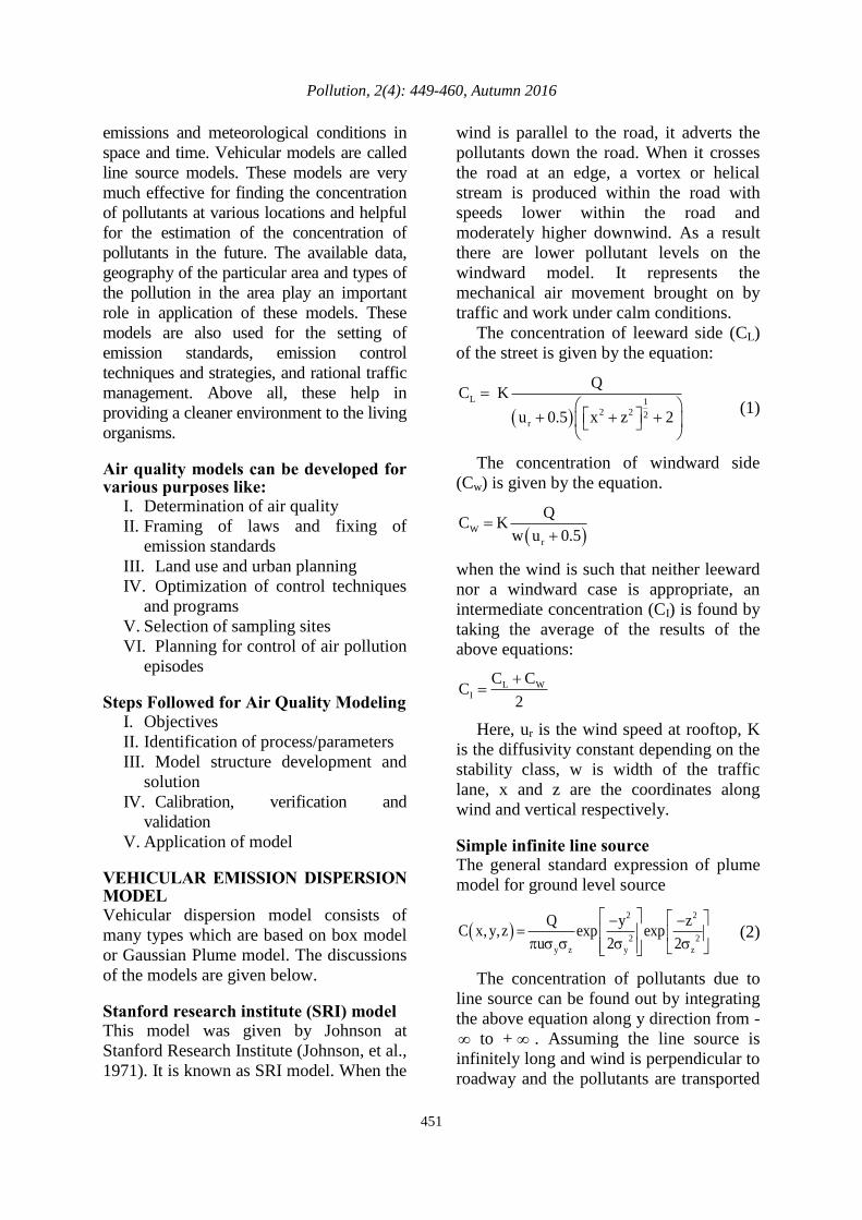
Stanford research institute (SRI) model This model was given by Johnson at
Stanford Research Institute (Johnson, et al.,
1971). It is known as SRI model. When the
wind is parallel to the road, it adverts the
pollutants down the road. When it crosses
the road at an edge, a vortex or helical
stream is produced within the road with
speeds lower within the road and
moderately higher downwind. As a result
there are lower pollutant levels on the
windward model. It represents the
mechanical air movement brought on by
traffic and work under calm conditions.
The concentration of leeward side (CL)
of the street is given by the equation:
r
L 12 2 2
Q
u 0.5 x z
2
C K
(1)
The concentration of windward side
(Cw) is given by the equation.
W
r
Q
w uC K
0.5
when the wind is such that neither leeward
nor a windward case is appropriate, an
intermediate concentration (CI) is found by
taking the average of the results of the
above equations:
LI
WC
2C
C
Here, ur is the wind speed at rooftop, K
is the diffusivity constant depending on the
stability class, w is width of the traffic
lane, x and z are the coordinates along
wind and vertical respectively.
Simple infinite line source The general standard expression of plume
model for ground level source
2 2
2 2
y z y z
C x, y,z exp expQ y z
u 2 2
(2)
The concentration of pollutants due to
line source can be found out by integrating
the above equation along y direction from -
to + . Assuming the line source is
infinitely long and wind is perpendicular to
roadway and the pollutants are transported
Kumar, A.
452
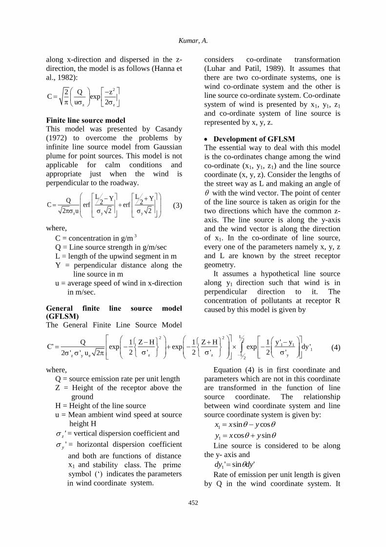
along x-direction and dispersed in the z-
direction, the model is as follows (Hanna et
al., 1982):
2
z z
2 Q zC exp
u 2
Finite line source model This model was presented by Casandy
(1972) to overcome the problems by
infinite line source model from Gaussian
plume for point sources. This model is not
applicable for calm conditions and
appropriate just when the wind is
perpendicular to the roadway.
z y y
L LY YQ 2 2erf erf2 u 2
C2
(3)
where,
C = concentration in g/m 3
Q = Line source strength in g/m/sec
L = length of the upwind segment in m
Y = perpendicular distance along the
line source in m
u = average speed of wind in x-direction
in m/sec.
General finite line source model (GFLSM) The General Finite Line Source Model
considers co-ordinate transformation
(Luhar and Patil, 1989). It assumes that
there are two co-ordinate systems, one is
wind co-ordinate system and the other is
line source co-ordinate system. Co-ordinate
system of wind is presented by x1, y1, z1
and co-ordinate system of line source is
represented by x, y, z.
Development of GFLSM The essential way to deal with this model
is the co-ordinates change among the wind
co-ordinate (x1, y1, z1) and the line source
coordinate (x, y, z). Consider the lengths of
the street way as L and making an angle of
with the wind vector. The point of center
of the line source is taken as origin for the
two directions which have the common z-
axis. The line source is along the y-axis
and the wind vector is along the direction
of x1. In the co-ordinate of line source,
every one of the parameters namely x, y, z
and L are known by the street receptor
geometry.
It assumes a hypothetical line source
along y1 direction such that wind is in
perpendicular direction to it. The
concentration of pollutants at receptor R
caused by this model is given by
L2 22
1 11
Lz z yz y e2
y' yQ 1 Z H 1 Z H 1exp exp exp dy'
2 ' 2 ' 2 '2 'C’
' u 2
(4)
where,
Q = source emission rate per unit length
Z = Height of the receptor above the
ground
H = Height of the line source
u = Mean ambient wind speed at source
height H
'z = vertical dispersion coefficient and
'y = horizontal dispersion coefficient
and both are functions of distance x1 and stability class. The prime
symbol (‘) indicates the parameters
in wind coordinate system.
Equation (4) is in first coordinate and
parameters which are not in this coordinate
are transformed in the function of line
source coordinate. The relationship
between wind coordinate system and line
source coordinate system is given by:
cossin1 yxx sincos1 yxy
Line source is considered to be along
the y- axis and
'sin'1 dydy Rate of emission per unit length is given
by Q in the wind coordinate system. It

Pollution, 2(4): 449-460, Autumn 2016
453
needs to be converted in the coordinate
system of line source where it would
become Q/sinθ because of the
transformation of the length unit, such that
the apparent length of the source Q is
multiplied by the factor 1/ sin because of
the obliquity of the source.
Substituting the value y1’, y1, x1, dy1’,
including the source correction in Equation
(4), the following equation is formed:
2 2
z zz y e
L22
1
2
L y2
Q 1 Z H 1 Z HC' exp exp
2 22 u 2
(y ' sin x cos ysin )exp sin dy '
2
(5)
Here y and z are the downwind
distance functions which are given by
sin/x and stability class. One sided
normal cumulative distribution function is
obtained from error function properties and
definition.
2
1
)exp( 2
f
f
dtt = .)()(2
12 ferfferf
Hence Equation (5) becomes:
2 2
z zz y e
y y
Q 1 Z H 1 Z Hexp exp
2 22 u 2
L Lsin Y x cos s
C
in Y x cos2 2
erf + erf2 2
(6)
where,
ue= usin + uo
uo= accounts for dispersion which is
lateral and concentration divergence when
wind speed coming towards zero (calm
condition, Luhar and Patil, 1989).
General motor (GM) model GM model was developed by Chock
(1978). It is used in line source approach
which is finite and one parameter of
dispersion is mentioned as a distance
function from line source and wind road
oriented angle. Importantly, it considers
plume rise over the roadways which are in
very stable and low wind conditions.
The concentration C at point (x,y) at y =
0 for line source is given by
2 2
0 0
z ze z
z h z hQ 1 1exp exp
2 2C
U 2
(7)
where,
h 0 = height of the plume centre above
the ground
The effective wind speed is given by
Ue = usin + uo
uo= correction factor for speed of wind
due to traffic wake
Ue = effective wind speed in m/sec.
The plume centre height is ho = H + hp
where H is height of line source and hp
is the plume rise.
EPA HIWAY model In EPA HIWAY Model (Petersen, 1980), a
highway is considered in which limited
point sources are assumed. The total
contribution due to all these points is found
out by taking out the integral of the

Kumar, A.
454
equation of point source by Gaussian for a
limited length L and incremental length of
dl, as given by:
fdlu
qlC (8)
If the condition is stable or if the height
of mixing is more than or same as 5000 m
then
2
2
2
2
2
2
2exp
2exp
2exp
2
1
zzyzy
HzHzyf
(9)
As the mechanical mixing is significant
over the street, some beginning estimations
of the vertical scattering and horizontal
scattering parameters are assumed by
displacement of the point source a virtual
separation upwind.
Integral is calculated by approximating
by the trapezoidal rule and gives:
1
1
21
2
n
i
ifff
u
qdlC
where if is evaluated from equation (9) for
l + dl .
California line source model Separate equation for the calculation of
concentrations of pollutants under
crosswind and parallel wind conditions is
used by the California model (Miller and
Clagget, 1978). Pollutant concentration is
calculated by the model in the crosswind
case by considering that the dispersion is
dependent on the atmospheric stability and
turbulent mixing cell is considered above
the highway.
CALINE 3 Model California Line Source Model Version 3
(CALINE-3) is an air quality model for
line source. It is a third generation model
established by California Department of
Transportation (Benson, 1992). It depends
on the equation of diffusion by Gaussian
and utilizes a mixing zone idea to describe
scattering of pollutants over the streets.
Each highway links are joined in a
progression of components and
incremental concentration is calculated.
After that this model adds all to get total
pollutant concentration on a specific
receptor area. The distance of receptor is a
perpendicular distance between receptor
and the highway centerline. Squares of
sides same as that of highway width are
taken as the first element formed at the
very first point.
With the distance from the receptor,
resolution of element becomes less
important. In order to permit efficiency in
computation the element is made larger.
Each component is taken as a "proportionate
limited line source" situated normal to the
direction of wind cantered in the mid-point
of element. A local x, y co-ordinate
framework adjusted to the direction of wind
and beginning at the component mid-point is
characterized for every component. The
emission occurring within the element is
modeled using the cross finite line source
Gaussian equation. The concentration due to
source segment of length dy is
2 22
2 2 2
y z y z z
z H z Hqdy ydc exp exp exp
2 u 2 2 2
(10)
where,
y , z diffusion coefficient in x and y
direction in m.
u the velocity of wind at effective
release height m/sec
he line source strength in µg/m/sec
he effective height of source in m
=
=
q= t
H= t
H= t

Pollution, 2(4): 449-460, Autumn 2016
455
dy he length of source segment in m
dc the concentration of the source
segment dy at receptor (x,y,z) in µg/m3.
In CALINE-3, region directly above the
road is treated as a region where the
emission is uniform. It defines the zone of
mixing as the region above the travelled
path including 3 m (approximately two-
vehicle width) on either side. The initial
horizontal dispersion is accounted by the
additional width imparted to the pollutant
by the vehicular wake. The model
considers pollutants to be inert. So it does
not consider the atmospheric reactions of
NOx (Benson, 1979).
AERMOD The AERMOD air dispersion model is
USEPAs official “Appendix A” air
dispersion model for regulatory use and was
developed by the AERMIC (The American
Meteorological Society/EPA Regulatory
Model Improvement Committee) work
group (Cimorelli et al., 2004). It is a steady-
state plume model. In the stable boundary
layer (SBL), it assumes the concentration
distribution to be Gaussian in both the
vertical and horizontal. In the convective
boundary layer (CBL), the horizontal
distribution is also assumed to be Gaussian,
but the vertical distribution is described with
a bi-Gaussian probability density function
(pdf).
AERMOD aims at modeling short-range
(up to 50 km) dispersion from a variety of
polluting sources (e.g., point, area, and
volume sources) using a number of model
configurations. These configurations
include different sets of urban or rural
dispersion coefficients as well as simple
and complex topography. The model has
the capacity to employ hourly sequential
pre-processed meteorological data to
estimate concentrations of pollutants at
receptor locations at different time scales
ranging from 1 h to 12 months. AERMOD
is an advanced plume model that
incorporates updated treatments of the
boundary layer theory, understanding of
turbulence and dispersion, and includes
handling of terrain interactions.
It has two pre-processors AERMET and
AERMAP. AERMET is a meteorological
pre-processor that calculates
meteorological parameters and passes them
to AERMOD. AERMAP is a terrain pre-
processor that calculates terrain elevations
above mean sea level and passes them to
AERMOD. It requires three kinds of input
data such as emission (vehicles),
geographical and meteorological data
(hourly nine meteorological parameters).
These hourly meteorological parameters
include Wind Speed, Wind Direction,
Ceiling Height, Rain Fall, Pressure,
Humidity, Global Horizontal Radiation,
Cloud Cover and Temperature. AERMOD
has been applied in many case studies for
vehicular pollution modeling (Kumar et al.,
2015; Sonawane et al., 2012).
Operational street pollution model (OSPM) The Operational Street Pollution Model
(OSPM) (Aquilina and Micallef, 2003) was
developed by the National Environmental
Research Institute of Denmark, Department
of Atmospheric Environment. It is an air
pollution model which is used for
foreseeing the scattering pollutants in
ambient air in road canyons. This model
has been utilized by various countries for
more than twenty years for examining level
of pollution due to traffic, performing
investigations of field campaign
estimations, considering effectiveness of
contamination reduction techniques, and
doing assessments of exposure. As
compared to different models OSPM is
cutting edge in traffic pollution modeling.
In OSPM amount of pollution due to
traffic is ascertained utilizing a mix of two
models. One is plume model for the
contribution which is direct. Second is a
box model for portion of pollutants which
is re-circulated in the road. The NO2
fixations are computed considering NO-
= t
=
Kumar, A.
456
NO2-O3 science and the time of residence
of contaminants on the road. This model is
intended to work with the input
information and then it gives one-hour
averages. OSPM has been applied in many
case studies for various purposes such as
source contribution and health impact
assessment in European cities (Aquilina
and Micallef, 2004; Assael et al., 2008;
Berkowicz et al., 2006; Berkowicz, 2000;
Berkowicz et al., 2008; Hvidberg and
Jensen, 2011; Kakosimos et al., 2010;
Ketzel et al., 2012; Kukkonen et al., 2001,
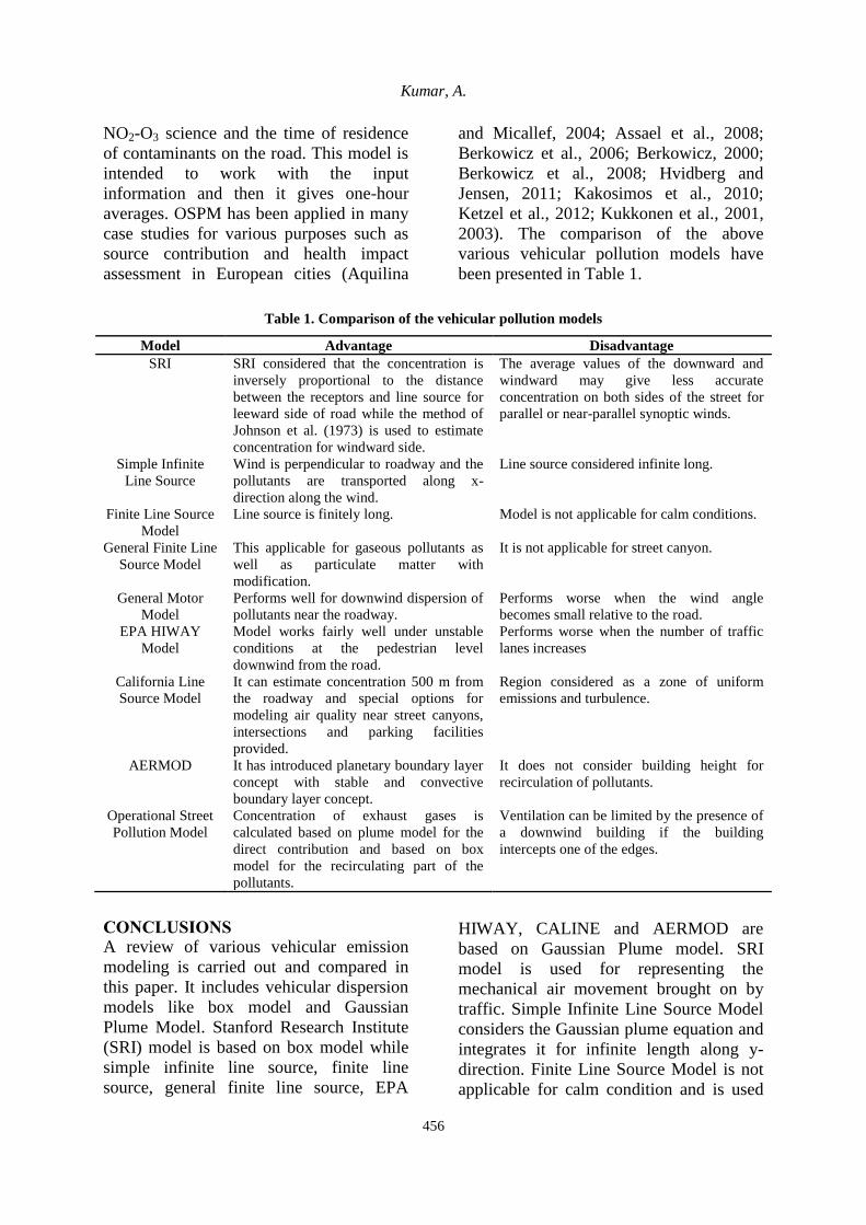
2003). The comparison of the above
various vehicular pollution models have
been presented in Table 1.
Table 1. Comparison of the vehicular pollution models
Model Advantage Disadvantage
SRI SRI considered that the concentration is
inversely proportional to the distance
between the receptors and line source for
leeward side of road while the method of
Johnson et al. (1973) is used to estimate
concentration for windward side.
The average values of the downward and
windward may give less accurate
concentration on both sides of the street for
parallel or near-parallel synoptic winds.
Simple Infinite
Line Source
Wind is perpendicular to roadway and the
pollutants are transported along x-
direction along the wind.
Line source considered infinite long.
Finite Line Source
Model
Line source is finitely long. Model is not applicable for calm conditions.
General Finite Line
Source Model
This applicable for gaseous pollutants as
well as particulate matter with
modification.
It is not applicable for street canyon.
General Motor
Model
Performs well for downwind dispersion of
pollutants near the roadway.
Performs worse when the wind angle
becomes small relative to the road.
EPA HIWAY
Model
Model works fairly well under unstable
conditions at the pedestrian level
downwind from the road.
Performs worse when the number of traffic
lanes increases
California Line
Source Model
It can estimate concentration 500 m from
the roadway and special options for
modeling air quality near street canyons,
intersections and parking facilities
provided.
Region considered as a zone of uniform
emissions and turbulence.
AERMOD It has introduced planetary boundary layer
concept with stable and convective
boundary layer concept.
It does not consider building height for
recirculation of pollutants.
Operational Street
Pollution Model
Concentration of exhaust gases is
calculated based on plume model for the
direct contribution and based on box
model for the recirculating part of the
pollutants.
Ventilation can be limited by the presence of
a downwind building if the building
intercepts one of the edges.
CONCLUSIONS A review of various vehicular emission
modeling is carried out and compared in
this paper. It includes vehicular dispersion
models like box model and Gaussian
Plume Model. Stanford Research Institute
(SRI) model is based on box model while
simple infinite line source, finite line
source, general finite line source, EPA
HIWAY, CALINE and AERMOD are
based on Gaussian Plume model. SRI
model is used for representing the
mechanical air movement brought on by
traffic. Simple Infinite Line Source Model
considers the Gaussian plume equation and
integrates it for infinite length along y-
direction. Finite Line Source Model is not
applicable for calm condition and is used

Pollution, 2(4): 449-460, Autumn 2016
457
only when the wind is perpendicular to the
roadway. However, there is no such
limitation in General Finite Line Source
Model as it considers co-ordinate
transformation. General Motor model
considers plume rise over the roadways
under very stable and low wind conditions.
EPA Highway model is a highway
dispersion model which considers a finite
number of point sources on the highway.
CALINE 3 is used for finding dispersion of
pollutants due to multiple highway links. It
considers diffusion by Gaussian and
utilizes a mixing zone idea to describe
scattering of pollutants over the streets. It
can be run for 8 hours period while
AERMOD where planetary boundary has
been introduced can be run for many years.
OSPM is used for predicting the scattering
of pollutants in road canyons between the
buildings. In OSPM, concentration of
exhaust gases is calculated based on plume
model for the direct contribution and based
on box model for the recirculating part of
the pollutants in the street. Nowadays,
CALINE3 and AERMOD are preferred for
finding dispersion on highways and widely
used for air quality management.
Future scope can be extended in several
ways. Many of them consider chemical
reactions for NOx but not for other
pollutants, so development of the model can
be extended to consider more chemical
reactions. The particulate matter (PM)
emission from tail pipe emission is low while
re-suspension of PM is caused by vehicle
movement. Generally, re-suspension of
particulate matter by vehicles is missed in
vehicular pollution modeling. Therefore, a
module of emission factor for re-suspension
of particulate matter can be developed and
incorporated in modeling. Canyon Street has
recirculation effect of pollutants from the
buildings which is captured by OSPM, but
this feature can also be enhanced in other
models. Meteorological data needed for air
quality modeling can be generated using
Weather Research Forecasting or other
meteorological model.
REFERENCES ARAI (2007). Air quality monitoring project-Indian
clean air programme (ICAP). “Emission Factor
development for Indian Vehicles”, ARAI, Pune,
India.
Aquilina, N. and Micallef, A. (2003). Evaluation of
the Operational Street Pollution Model Using Data
from European Cities. Env. Mont Asses., 95, 75-96.
Assael, M.J.Ã., Delaki, M. & Kakosimos, K.E. (2008).
Applying the OSPM model to the calculation of PM
10 concentration levels in the historical centre of the
city of Thessaloniki. Atmospheric Environment, 42,
65–77. doi:10.1016/j.atmosenv.2007.09.029.
Alves, C.A., Gomes, J., Nunes, T., Duarte, M.,
Calvo, A., Custódio, D., Pio, C., Karanasiou, A. and
Querol, X. (2014). Size-segregated particulate
matter and gaseous emissions from motor vehicles
in a road tunnel. Atmos. Res. 153, 134–144.
doi:10.1016/j.atmosres.2014.08.002.
Banerjee, T., Barman, S.C. and Srivastava, R.K.
(2011). Application of air pollution dispersion
modeling for source-contribution assessment and
model performance evaluation at integrated
industrial estate-Pantnagar. Environmental pollution
(Barking, Essex : 1987), 159(4), 865–75.
doi:10.1016/j.envpol.2010.12.026.
Barratt, R. (2000). Atmospheric dispersion
modeling- An introduction to practical applications,
Business and Environment Practitioner Series,
Earthscan Publications Limited, London (UK).
Berkowicz, R. (2000). OSPM- a parameterised
street pollution model. Environmental monitoring
and assessment, 65, 323–331.
Benson, P.E. (1992). A review of the development
and application of the CALINE 3 and 4 models.
Atmos. Env. 26B (3), 379-390.
Benson, P.E. (1979). CALINE -3: A versatile
dispserion model for prediction air pollutant levels
near highways and arterial roads. Final Report.
FHWA/CA/TL-79/23 California Department of
Transportation, Sacramento, CA.
Berkowicz, R., Ketzel, M., Solvang, S., Hvidberg,
M. and Raaschou-nielsen, O. (2008). Evaluation
and application of OSPM for traffic pollution
assessment for a large number of street locations.
Environmental Modeling & Software, 23, 296–303.
doi:10.1016/j.envsoft.2007.04.007.
Berkowicz, R., Winther, M. and Ketzel, M. (2006).
Traffic pollution modeling and emission data.

Kumar, A.
458
Environmental Modeling & Software, 21(4), 454–
460. doi:10.1016/j.envsoft.2004.06.013.
Brandt, J., Silver, J.D., Christensen, J.H., Andersen,
M.S., Bønløkke, J.H., Sigsgaard, T., et al. (2013).
Assessment of past, present and future health-cost
externalities of air pollution in Europe and the
contribution from international ship traffic using the
EVA model system. Atmospheric Chemistry and
Physics, 13(15), 7747–7764. doi:10.5194/acp-13-
7747-2013.
Briggs, D.J., Hough. D., Gulliver, W., Elliott, P.,
Kingham, S. and Small Bone, K. (2000). A
regression-based method for mapping traffic-related
air pollution: application and testing in four
contrasting urban environments. Sci. of The Tot.
Env., 253(1-3), 151-67.
Brzezinski, D.J. and Newell, T.P. (2000). A
Revised Model for Estimation of Highway Vehicle
Emissions. Air Waste Manag. Assoc. EPA420-S-9,
1–18.
Casandy, G.T. (1972). Crosswind Shear Effect on
Atmospheric Diffusion. Atmos. Env., 6, 221-232.
Cassidy, T., Inglis, G., Wiysonge, C. and
Matzopoulos, R. (2014). Health & Place A systematic
review of the effects of poverty deconcentration and
urban upgrading on youth violence. Health & Place,
26, 78–87. doi:10.1016/j.healthplace.2013.12.009.
Cheng, S., Lang, J., Zhou, Y., Han, L., Wang, G.
and Chen, D. (2013). A new monitoring-simulation-
source apportionment approach for investigating the
vehicular emission contribution to the PM2.5
pollution in Beijing, China. Atmos. Environ. 79,
308–316. doi:10.1016/j.atmosenv.2013.06.043.
Chock, D.P. (1978). A line source model for
dispersion near Roadways. Atmos. Env., 12, 823–829.
Cimorelli, A.J., Perry, S.G., Venkatram, A., Weil,
J.C., Paine, R.J., Wilson, Robert, B., et al. (2004).
AERMOD : Description of Model Formulation.
EPA-454/R-03-004, USEPA, USA.
Coelho, M.C., Fontes, T., Bandeira, J.M., Pereira,
S.R., Tchepel, O., Dias, D., Sá, E., Amorim, J.H. and
Borrego, C. (2014). Assessment of potential
improvements on regional air quality modeling related
with implementation of a detailed methodology for
traffic emission estimation. Sci. Total Environ. 470-
471, 127–137. doi:10.1016/j.scitotenv.2013.09.042.
CPCB (2001). Vehicular Pollution Control in India,
Technical and Non-Technical Measure Policy.
Cent. Pollut. Control Board, Minist. Environemntal
For. Gov. India.
Fan, X., Lam, K.C. and Yu, Q. (2012). Differential
exposure of the urban population to vehicular air
pollution in Hong Kong. Science of the Total
Environment, 426, 211–219.
doi:10.1016/j.scitotenv.2012.03.057.
Fensterstock, J.C., Kurtzweg, J.A. and Ozolins, G.
(1971). Reduction of Air Pollution Potential
through Environmental Planning, Journal of the Air
Pollution Control Association 21(7), 395-399. DOI:
10.1080/00022470.1971.10469547.
Fenger, J. (2009). Air pollution in the last 50 years -
From local to global. Atmos. Env., 43(1), 13–22.
doi:10.1016/j.atmosenv.2008.09.061.
Fridell, E., Haeger-Eugensson, M., Moldanova, J.,
Forsberg, B. and Sjöberg, K. (2014). A modeling
study of the impact on air quality and health due to
the emissions from E85 and petrol fuelled cars in
Sweden. Atmospheric Environment, 82, 1–8.
doi:10.1016/j.atmosenv.2013.10.002.
Gulia, S., Shiva Nagendra, S.M., Khare, M. and
Khanna, I. (2015). Urban air quality management- a
review. Atmospheric Pollution Research, 6(2), 286–
304. doi:10.5094/APR.2015.033.
Guttikunda, S.K. and Goel, R. (2013). Health
impacts of particulate pollution in a megacity-Delhi,
India. Environ. Dev. 6, 8–20.
doi:10.1016/j.envdev.2012.12.002.
Hanna, S.R., Briggs, G.A. and Hosker, P.R. (1982).
Handbook on Atmospheric Diffusion, Technical
information centre USDOE Chapter 9: 59-60.
Hvidberg, M. and Jensen, S.S. (2011). Evaluation of
AirGIS : a GIS-based air pollution and human
exposure modeling system Matthias Ketzel, Ruwim
Berkowicz, Ole Raaschou-Nielsen. International
Journal of Environment and Pollution, 47, 226–238.
Ilyas, Z.S., Khattak, A.I., Nasir, S.M., Qurashi, T. and
Durrani, R. (2010). Air pollution assessment in urban
areas and its impact on human health in the city of
Quetta, Pakistan. Clean Techn Environ Policy, 12,
291–299. doi:10.1007/s10098-009-0209-4.
Jiang, P., Chen, Y., Geng, Y., Dong, W., Xue, B.,
Xu, B. and Li, W. (2013). Analysis of the co-bene fi
ts of climate change mitigation and air pollution
reduction in China. J. of Cleaner Production, 58,
130–137. doi:10.1016/j.jclepro.2013.07.042.
Jiménez-guerrero, P., Jorba, O., Baldasano, J. M. and
Gassó, S. (2007). The use of a modeling system as a
tool for air quality management : Annual high-
resolution simulations and evaluation. Science of the
Total Environment, 390, 323–340.
doi:10.1016/j.scitotenv.2007.10.025.
Jin, S. and Demerjian, K. (1993). A Photochemical
Box Model for Urban Air Quality Study.
Atmospheric Environment, 27B(4), 371–387.

Pollution, 2(4): 449-460, Autumn 2016
459
Johnson, W.B., Ludwig, F.L., Dabbrdt, W.F. and
Allen, R.J. (1971). Field study for an initial
evaluation of an urban diffusion model for carbon
monoxide. Comprehensive Report For Coordinating
Research Institute and EPA Contract. Stanford
Research Institute, Milano park, Calinfornia.
CAPA-3-68, 1-69.
Kakosimos, K.E., Hertel, D.O. and B.C.M.K. (2010).
Operational Street Pollution Model (OSPM)– a review
of performed application and validation studies, and
future prospects. Environmental Chemistry, 7, 485–
503. doi:10.1071/EN10070.
Kampa, M. and Castanas, E. (2008). Human health
effects of air pollution. Environmental Pollution,
151(2), 362–367. doi:10.1016/j.envpol.2007.06.012.
Kan, H., Chen, R. and Tong, S. (2012). Ambient air
pollution, climate change, and population health in
China. Environment international, 42, 10–9.
doi:10.1016/j.envint.2011.03.003.
Kan, H., Huang, W., Chen, B. and Zhao, N. (2009).
Impact of outdoor air pollution on cardiovascular
health in Mainland China. CVD Prevention and
Control, 4(1), 71–78.
doi:10.1016/j.cvdpc.2008.08.004.
Kesarkar, A.P., Dalvi, M., Kaginalkar, A. and Ojha, A.
(2007). Coupling of the Weather Research and
Forecasting Model with AERMOD for pollutant
dispersion modeling. A case study for PM10
dispersion over Pune, India. Atmospheric
Environment, 41(9), 1976–1988.
doi:10.1016/j.atmosenv.2006.10.042.
Ketzel, M., Ss, J., Brandt, J., Ellermann, T., Hr, O.,
Berkowicz, R. and Hertel, O. (2012). Evaluation of
the Street Pollution Model OSPM for
Measurements at 12 Streets Stations Using a Newly
Developed and Freely Available Evaluation Tool.
Civil & Environmental Engineering, S1:004, 1–11.
doi:10.4172/2165-784X.S1-004.
Kukkonen, J., Partanen, L., Karppinen, A. and
Walden, J. (2003). Evaluation of the OSPM model
combined with an urban background model against
the data measured in 1997 in Runeberg Street,
Helsinki. Atmospheric Environment, 37, 1101–
1112. doi:10.1016/S1352-2310(02)00957-3.
Kukkonen, J., Valkonen, E., Walden, J.,
Koskentalo, T., Aarnio, K., Karppinen, A., et al.
(2001). A measurement campaign in a street canyon
in Helsinki and comparison of results with
predictions of the OSPM model. Atmospheric
Environment, 35, 231–243.
Kumar, A., Dikshit, A.K., Fatima, S., Patil, R.S.
(2015). Application of WRF model for vehicular
pollution modeling using AERMOD. Atmos. and
Cli. Sci., 5, 57–62.
Krewski, D. and Rainham, D. (2007). Ambient Air
Pollution and Population Health : Overview.
Journal of Toxicology and Environmental Health,
Part A, 70, 275–283.
doi:10.1080/15287390600884859.
Kristiansson, M., Sörman, K., Tekwe, C. and
Calderón-garcidueñas, L. (2015). Urban air pollution,
poverty, violence and health – Neurological and
immunological aspects as mediating factors.
Environmental Research, 140, 511–513.
doi:10.1016/j.envres.2015.05.013.
Lai, A.C.K., Thatcher, T.L. and Nazaroff, W.W.
(2012). Inhalation Transfer Factors for Air Pollution
Health Risk Assessment. Journal of the Air &
Waste Management Association, 50, 1688–1699.
doi:10.1080/10473289.2000.10464196.
Luhar, A.K. and Patil, R.S. (1989). A General Finite
Line Source Model For Vehicular Pollution
Prediction” Atmos. Env., 23, 555-562.
Maantay, J. (2007). Asthma and air pollution in the
Bronx: methodological and data considerations in
using GIS for environmental justice and health
research. Health & place, 13(1), 32–56.
doi:10.1016/j.healthplace.2005.09.009.
Ma, J., Yi, H., Tang, X., Zhang, Y., Xiang, Y. and Pu,
L. (2013). Application of AERMOD on near future air
quality simulation under the latest national emission
control policy of China: A case study on an industrial
city. Journal of Environmental Sciences, 25(8), 1608–
1617. doi:10.1016/S1001-0742(12)60245-9.
Marquez, L.O. and Smith, N.C. (1999). A
framework for linking urban form and air quality.
Environmental Modeling & Software, 14(6), 541–
548. doi:10.1016/S1364-8152(99)00018-3.
Martins, H. (2012). Urban compaction or
dispersion? An air quality modeling study.
Atmospheric Environment, 54, 60–72.
doi:10.1016/j.atmosenv.2012.02.075.
Miller, T.L. and Clagget, M. (1978). A Comparison
of Three Highway Line Source Dispersion Models.
Atmos. Env., 12, 1323-1329.
Mokhtar, M.M., Hassim, M.H. and Taib, R.M.
(2014). Health risk assessment of emissions from a
coal-fired power plant using AERMOD modeling.
Process Safety and Environmental Protection, 92,
476–485.
Ozkurt, N., Sari, D., Akalin, N. and Hilmioglu, B.
(2013). Evaluation of the impact of SO2 and NO2
emissions on the ambient air-quality in the ??an-
Bayrami?? region of northwest Turkey during
Kumar, A.
460
2007-2008. Science of the Total Environment, 456-
457(2), 254–266.
doi:10.1016/j.scitotenv.2013.03.096.
Pandey, J.S., Kumar, R. and Devotta, S. (2005).
Health risks of NO2, SPM and SO2 in Delhi
(India). Atmospheric Environment, 39(36), 6868–
6874. doi:10.1016/j.atmosenv.2005.08.004.
Patankar, A.M. and Trivedi, P.L. (2011). Monetary
burden of health impacts of air pollution in
Mumbai, India: implications for public health
policy. Public health, 125(3), 157–64.
doi:10.1016/j.puhe.2010.11.009.
Petersen, W. (1980). A Highway Air Pollution Model,
User's guide for HIWAY2, U.S. Environmental
Protection Agency, Research Triangle Park, North
Carolina, EPA-600/8-80-018, 69 p.
Rao, S., Pachauri, S., Dentener, F., Kinney, P.,
Klimont, Z., Riahi, K. and Schoepp, W. (2013).
Better air for better health: Forging synergies in
policies for energy access, climate change and air
pollution. Global Environmental Change, 23(5),
1122–1130. doi:10.1016/j.gloenvcha.2013.05.003.
Ritter, M., Müller, M.D., Tsai, M.Y. and Parlow, E.
(2013). Air pollution modeling over very complex
terrain: An evaluation of WRF-Chem over
Switzerland for two 1-year periods. Atmospheric
Research, 132-133, 209–222.
doi:10.1016/j.atmosres.2013.05.021.
Sellier, Y., Galineau, J., Hulin, A., Caini, F.,
Marquis, N., Navel, V., et al. (2014). Health effects
of ambient air pollution: do different methods for
estimating exposure lead to different results?
Environment international, 66, 165–73.
doi:10.1016/j.envint.2014.02.001.
Sivacoumar, R. and Thanasekaran, K. (1999). Line
source model for vehicular pollution prediction near
roadways and model evaluation through statistical
analysis. Environ. Poll., 104, 389–395.
doi:10.1016/S0269-7491(98)00190-0.
Sonawane, N.V., Patil, R.S. and Sethi, V. (2012).
Health benefit modeling and optimization of vehicular
pollution control strategies. Atmos. Environ. 60, 193–
201. doi:10.1016/j.atmosenv.2012.06.060.
Spickett, J., Katscherian, D. and Harris, P. (2013).
The role of Health Impact Assessment in the setting
of air quality standards : An Australian perspective.
Environmental Impact Assessment Review, 43, 97–
103. doi:10.1016/j.eiar.2013.06.001.
Srivastava, A. and Kumar, R. (2002). Economic
valuation of health impacts of air pollution in mumbai.
Environmental monitoring and assessment, 75, 135–
143.
Singh, N.P. and Gokhale, S. (2015). A method to
estimate spatiotemporal air quality in an urban
traffic corridor. Sci. of the Tot. Env., 538, 458–467.
Syrakov, D., Prodanova, M., Georgieva, E.,
Etropolska, I. and Slavov, K. (2015). Simulation of
European air quality by WRF–CMAQ models using
AQMEII-2 infrastructure. Journal of Computational
and Applied Mathematics.
doi:10.1016/j.cam.2015.01.032.
Thaker, P. and Gokhale, S. (2015). The impact of
traffic- fl ow patterns on air quality in urban street
canyons. Environmental Pollution, in press.
Whitworth, K.W., Symanski, E., Lai, D. and Coker,
A.L. (2011). Kriged and modeled ambient air levels
of benzene in an urban environment : an exposure
assessment study. Environmental Health, 10(1), 21.
doi:10.1186/1476-069X-10-21.
Yan, F., Winijkul, E., Jung, S., Bond, T.C. and
Streets, D.G. (2011). Global emission projections of
particulate matter (PM): I. Exhaust emissions from
on-road vehicles. Atmos. Environ. 45, 4830–4844.
doi:10.1016/j.atmosenv.2011.06.018.
Zhang, H., Chen, G., Hu, J., Chen, S., Wiedinmyer,
C., Kleeman, M. and Ying, Q. (2014). Evaluation of
a seven-year air quality simulation using the
Weather Research and Forecasting (WRF)/
Community Multiscale Air Quality (CMAQ)
models in the eastern United States, Science of the
Total Environment 474, 275–285.
Pollution is licensed under a "Creative Commons Attribution 4.0 International (CC-BY 4.0)"