Vehicular Pollution Control – Concept note

Dr. Vinish Kathuria Associate Professor

vinish@mse.ac.in; vinish67@yahoo.com

Madras School of Economics

Gandhi Mandapam Road Chennai 600 025

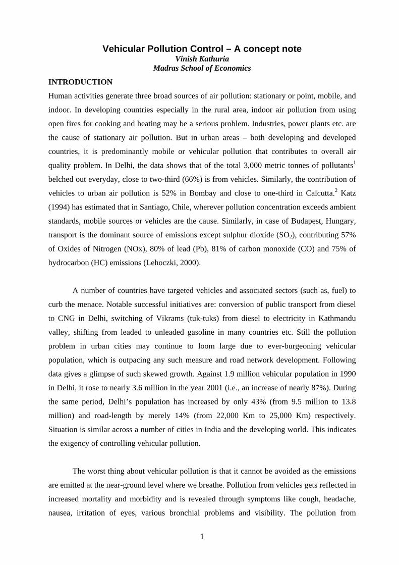
Vehicular Pollution Control – A concept note Vinish Kathuria

Madras School of Economics

INTRODUCTION

Human activities generate three broad sources of air pollution: stationary or point, mobile, and

indoor. In developing countries especially in the rural area, indoor air pollution from using

open fires for cooking and heating may be a serious problem. Industries, power plants etc. are

the cause of stationary air pollution. But in urban areas – both developing and developed

countries, it is predominantly mobile or vehicular pollution that contributes to overall air

quality problem. In Delhi, the data shows that of the total 3,000 metric tonnes of pollutants1

belched out everyday, close to two-third (66%) is from vehicles. Similarly, the contribution of

vehicles to urban air pollution is 52% in Bombay and close to one-third in Calcutta.2 Katz

(1994) has estimated that in Santiago, Chile, wherever pollution concentration exceeds ambient

standards, mobile sources or vehicles are the cause. Similarly, in case of Budapest, Hungary,

transport is the dominant source of emissions except sulphur dioxide (SO2), contributing 57%

of Oxides of Nitrogen (NOx), 80% of lead (Pb), 81% of carbon monoxide (CO) and 75% of

hydrocarbon (HC) emissions (Lehoczki, 2000).

A number of countries have targeted vehicles and associated sectors (such as, fuel) to

curb the menace. Notable successful initiatives are: conversion of public transport from diesel

to CNG in Delhi, switching of Vikrams (tuk-tuks) from diesel to electricity in Kathmandu

valley, shifting from leaded to unleaded gasoline in many countries etc. Still the pollution

problem in urban cities may continue to loom large due to ever-burgeoning vehicular

population, which is outpacing any such measure and road network development. Following

data gives a glimpse of such skewed growth. Against 1.9 million vehicular population in 1990

in Delhi, it rose to nearly 3.6 million in the year 2001 (i.e., an increase of nearly 87%). During

the same period, Delhi’s population has increased by only 43% (from 9.5 million to 13.8

million) and road-length by merely 14% (from 22,000 Km to 25,000 Km) respectively.

Situation is similar across a number of cities in India and the developing world. This indicates

the exigency of controlling vehicular pollution.

The worst thing about vehicular pollution is that it cannot be avoided as the emissions

are emitted at the near-ground level where we breathe. Pollution from vehicles gets reflected in

increased mortality and morbidity and is revealed through symptoms like cough, headache,

nausea, irritation of eyes, various bronchial problems and visibility. The pollution from

1

vehicles are due to discharges like CO, unburned HC, Pb compounds, NOx, soot, suspended

particulate matter (SPM) and aldehydes, among others, mainly from the tail pipes. A recent

study reports that in Delhi one out of every 10 school children suffers from asthma that is

worsening due to vehicular pollution.3 Similarly, two of the three most important health related

problems in Bangkok are caused by air pollution and lead contamination, both of which are

contributed greatly by motor vehicles.4 Situation is same in a number of other mega-cities

across the globe – be it Mexico City, Sao Paulo and Santiago in Latin America or Bangkok,

Jakarta, Manila, Dhaka in Asia or Ibadan and Lagos in Africa or in cities of Eastern Europe,

the erstwhile USSR and the Middle East. According to the World Health Organisation (WHO),

4 to 8% of deaths that occur annually in the world are related to air pollution and of its

constituents, the WHO has identified SPM as the most sinister in terms of its effect on health.

The SPM is not homogeneous. It has a number of constituents. As a result, it is

measured and characterised in various ways: (i) TSP (Total suspended particulates) with

particle diameters < 50-100 µm is the fraction sampled with high-volume samplers. (ii) PM :

Inhalable particles having a diameter <10 µm penetrates through the nose, by breathing. (iii)

Thoracic particles: are approximately equal to PM particles. (iv) PM : ‘Fine fraction’ with a

diameter <2.5 µm penetrates to the lungs; and (v) Black smoke: a measure of the blackness of

a particle sample gives a relative value for the soot content of the sample. Due to their high

health damaging potential

10

10 2.5

recent studies have started paying more attention to PM10 and PM2.5

particles.5

The different air pollutants due to vehicles can have effects at all the three levels – local

(e.g., smoke affecting visibility, ambient air, noise etc.), regional (such as smog, acidification)

and global (i.e., global warming). The vehicles besides being the prominent source of air

pollutants also account for a number of external effects, such as congestion, noise, accidents,

road wear and tear, and ‘barrier effects’.6

Under this background this note investigates what is the economics of vehicular

pollution control and what policy instruments / initiatives can be employed to control the

vehicular pollution. For a prescription to yield desired results, it should hit the right source of

pollution. Section 2 gives in brief the contribution of different sources to vehicular air pollution

problem. This is followed by the economics of vehicular pollution control in Section 3. The

section also explores the instruments that can be applied to control vehicular pollution. The

2

major difference between developing and developed countries lies in the fact that institutions

are in place and information of health impacts are known to the policy makers. For developing

countries, the challenge rests on devising suitable policy instruments that fully take into

account the damage caused by the polluting source. A discussion of complexity involved in

estimating the damage function is given in Section 4. Section 5 gives under what conditions a

particular instrument will be more appropriate, especially in the case of mega cities of

developing world followed by India’s experience in combating vehicular pollution. The

concept note concludes in Section 6. It is to be stated at the outset that the note covers mainly

the environmental consequences of transport and does not investigate the other important

external effects of the sector such as barrier effect, congestion effect etc.

VEHICULAR AIR POLLUTION – CAUSES OF EMISSIONS7

Vehicular pollution sources are not homogenous, as there is a complete range of technological

mix. The mix could be in terms of fuel used – gasoline or diesel or natural gas; or engine type

– 2-stroke or 4-stroke and/or a combination of these.

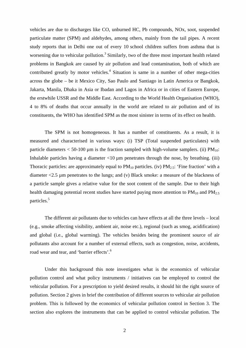
Emissions from Gasoline Vehicles Gasoline-powered engines are of two types: 4-stroke and 2-stroke. Table 1 gives the various

sources of emissions in the two cases. The exhaust emissions from gasoline-run vehicles

consist of CO, HC, NOx, SO2, and partial oxides of aldehydes, besides particulate matters

including lead salts.

Table 1: Emission from Gasoline Vehicles Amount of Emissions (%) Remarks Source 4-stroke 2-stroke

1 Crankase blowby 20 0 Carburreted air-fuel mixture & combustion fuel under pressure escape combustion chamber past engine piston and ring and enter crankbase to be discharged into atmosphere through vents

2 Evaporative Emissions

20 3 Fuel vapours lost to the atmosphere from tanks and carburettor

3 Exhaust Emissions 60 97 Exhaust gases emitted with pollutants through the tailpipe

Source: CPCB (1999)

The incomplete combustion of gasoline due to an imbalance in the air-fuel ratio leads

to emissions of CO and HC especially from 2-stroke engines. The Nox, however, are formed

due to high combustion temperature and availability of oxygen and nitrogen in the combustion

chamber, whereas aldehydes result from the partial oxidation of HC. In cities, majority of the

3

pollution is emitted by vehicles consuming gasoline − especially 2 and 3-wheelers, having

predominantly 2-stroke engine.

The 2-stroke 2- and 3-wheelers require 2 T oil for lubrication of engine, which is

carried out through either premixing mode or oil injection system. In either case it is a total

loss system, as the oil is burnt along with the fuel. Since the burning quality of mineral based

lubricating oil is very poor vis-à-vis gasoline, major fraction of it that enters the engine either

remains unburned or burns only partially. This unburned and partially burned oil comes

through the exhaust and is responsible for smoke and SPM emission. The studies indicate that

2-stroke engine’s exhaust contains almost 15-25% of unburned fuel (Pundir, 2001). In actual

practice, the 2-stroke vehicles require 2% concentration of 2 T oil i.e., 20 ml in a litre of petrol

and even a modest 1% increase of oil, may lead to 15% increase in SPM besides visible smoke

(CPCB, 1999). In most growing cities − Delhi, Kathmandu, Chennai, Dhaka, Pune etc. −

gasoline or petrol driven vehicles comprise over 80% of the total vehicles registered. This

implies controlling pollution from them can have significant pay-offs.

Emissions from Diesel Vehicles

As diesel engines breathe only air, blowby gases from the crankcase (consisting primarily of

air and HC) are rather low. Due to its low volatility, evaporative emissions from the fuel tank

can also be ignored. The low concentration of CO and un-burnt HC in the diesel exhaust are

compensated by high concentration of NOx. Diesel engines also emit smoke particles and

oxygenated HC, including aldehydes and odour-producing compounds having high nuisance

value.

Smoke from diesel engines comes in three different hues – white smoke emitted during

cold start idling and at low loads; blue smoke from the burning of lubricating oil and additives;

and black smoke, a product of incomplete combustion. Black smoke, the most obvious type of

vehicular air pollution, consists of irregular shaped agglomerated fine soot/particulates, the

formation of which depends on injector nozzle parameter and type of combustion chamber

(direct or indirect injection). Black smoke is a particular problem with diesel engines that are

not well tuned, which is often the case in the developing world.

4

Impact of (Gasoline and Diesel) Fuel Quality on emissions

Much of the pollution control depends on the quality of the fuel. So the characteristics that

determine fuel quality also become important. A high Reid pressure8 in the case of gasoline

engine causes a high evaporative emission while an increase in the density results in a

simultaneous increase in CO and HC in the exhausts. Likewise in the case of diesel vehicles, a

higher density causes higher smoke, CO and NOx emissions, while enhancing the cetane

number9 of ignition quality lowers the smoke emission. The sulphur content of diesel has been

observed to have a direct bearing on the SPM and SO2 emissions (CPCB, 1999).

Pollutants from Diesel vis-à-vis CNG Run Engines

The combustion of fuels release SO2, NOx, CO and ozone. The CO is highly noxious gas that

forms when there is not enough oxygen during the combustion. The CO, however, oxidizes

very fast and forms CO2, which though is not noxious but is one of the major contributors of

greenhouse effect. This implies a reduction of CO, hence CO2 emissions, can only be achieved

by improving the engine efficiency or by using fuels containing lower concentration of carbon

such as natural gas.

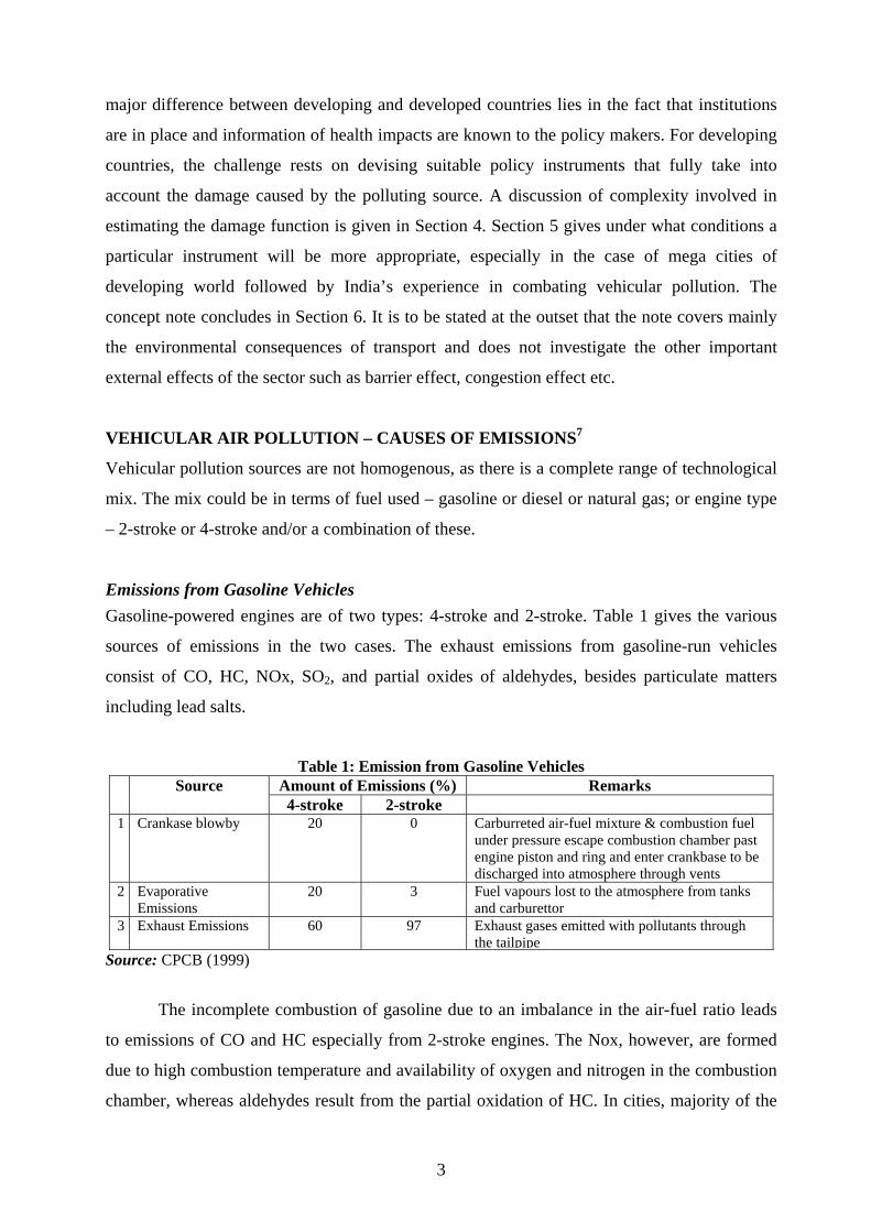
The compressed natural gas (CNG) is a clean-burning alternative fuel for vehicles10

with a significant potential for reducing harmful emissions especially fine particles. Nylund

and Lawson (2000) find that diesel combustion emits 84 grams per kilometer (gms/km) of such

components as compared to only 11 gms/km in CNG. The levels of greenhouse gases emitted

from natural gas exhaust are 12% lower than diesel engine exhaust when the entire life cycle of

the fuel is considered (ibid.). It has also been found that one CNG bus achieves emission

reduction equivalent to removing 85-94 cars from the road. Table 2 gives the emission benefits

of replacing conventional diesel with CNG in buses.

Table 2: Emission Benefits of Replacing Conventional Diesel with CNG in Buses Pollution Parameter Fuel

CO NOx PM Diesel 2.4 g/km 21 g/km 0.38 g/km CNG 0.4 g/km 8.9 g/km 0.012 g/km % Reduction 84 58 97

Source: Frailey et al. (2000) as referred in World Bank (2001b: 2).

Diesel with sulphur content of 10 ppm (also called as ‘clean diesel’) is environmentally

viable only when it is combined with other technology such as the state of the art exhaust

5

treatment devices like continuously regenerating particulate traps (CRTs). Incidentally the

devices are also highly maintenance intensive.

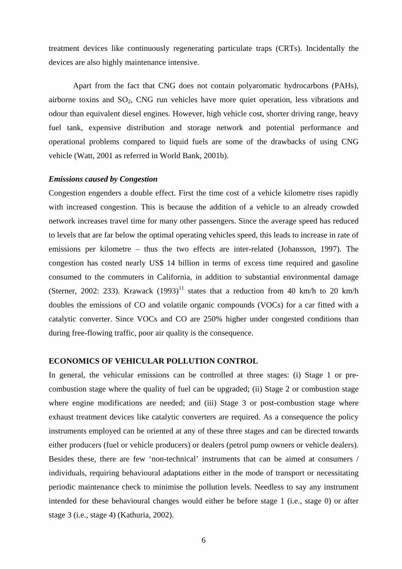
Apart from the fact that CNG does not contain polyaromatic hydrocarbons (PAHs),

airborne toxins and SO2, CNG run vehicles have more quiet operation, less vibrations and

odour than equivalent diesel engines. However, high vehicle cost, shorter driving range, heavy

fuel tank, expensive distribution and storage network and potential performance and

operational problems compared to liquid fuels are some of the drawbacks of using CNG

vehicle (Watt, 2001 as referred in World Bank, 2001b).

Emissions caused by Congestion

Congestion engenders a double effect. First the time cost of a vehicle kilometre rises rapidly

with increased congestion. This is because the addition of a vehicle to an already crowded

network increases travel time for many other passengers. Since the average speed has reduced

to levels that are far below the optimal operating vehicles speed, this leads to increase in rate of

emissions per kilometre – thus the two effects are inter-related (Johansson, 1997). The

congestion has costed nearly US$ 14 billion in terms of excess time required and gasoline

consumed to the commuters in California, in addition to substantial environmental damage

(Sterner, 2002: 233). Krawack (1993)11 states that a reduction from 40 km/h to 20 km/h

doubles the emissions of CO and volatile organic compounds (VOCs) for a car fitted with a

catalytic converter. Since VOCs and CO are 250% higher under congested conditions than

during free-flowing traffic, poor air quality is the consequence.

ECONOMICS OF VEHICULAR POLLUTION CONTROL

In general, the vehicular emissions can be controlled at three stages: (i) Stage 1 or pre-

combustion stage where the quality of fuel can be upgraded; (ii) Stage 2 or combustion stage

where engine modifications are needed; and (iii) Stage 3 or post-combustion stage where

exhaust treatment devices like catalytic converters are required. As a consequence the policy

instruments employed can be oriented at any of these three stages and can be directed towards

either producers (fuel or vehicle producers) or dealers (petrol pump owners or vehicle dealers).

Besides these, there are few ‘non-technical’ instruments that can be aimed at consumers /

individuals, requiring behavioural adaptations either in the mode of transport or necessitating

periodic maintenance check to minimise the pollution levels. Needless to say any instrument

intended for these behavioural changes would either be before stage 1 (i.e., stage 0) or after

stage 3 (i.e., stage 4) (Kathuria, 2002).

6

The standard externality diagram given in Figure 1 provides the intuition how the

various policy options work. The existing / potential users of (polluting) transport (say car or

2-wheelers) will use transport services up to the point where the benefits they derive, as

represented by their demand schedule is equated with the additional costs (called as marginal

costs in economics) they have to incur. This yields an equilibrium traffic volume, Ta. At this

equilibrium traffic volume, users equate only their private costs of running the vehicle with the

benefits they derive from the use of the vehicle (i.e., Pa). However, the users do not take into

account the environmental and other costs they impose on others by increasing the air pollution

or by crowding the roads or by driving poorly maintained vehicles. In other words, there is a

complete divergence between private costs, which users bear and the social costs of driving the

vehicle, i.e. a negative externality given by Po1 – Pa. If the users are forced to internalise this

external cost, the effect will be equivalent to the optimal (limited/reduced) traffic volume, To at

a cost of Po to the individuals. The regulator has a number of ways – called as policy

instruments – to achieve this optimal traffic that internalises this negative externality – by

regulations, subsidies, taxes, incentives etc.

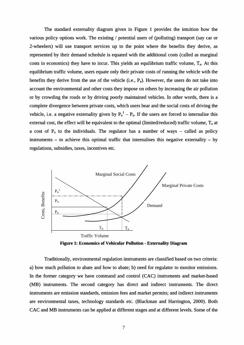
The standard externality diagram given in Figure 1 provides the intuition how the

various policy options work. The existing / potential users of (polluting) transport (say car or

2-wheelers) will use transport services up to the point where the benefits they derive, as

represented by their demand schedule is equated with the additional costs (called as marginal

costs in economics) they have to incur. This yields an equilibrium traffic volume, Ta. At this

equilibrium traffic volume, users equate only their private costs of running the vehicle with the

benefits they derive from the use of the vehicle (i.e., Pa). However, the users do not take into

account the environmental and other costs they impose on others by increasing the air pollution

or by crowding the roads or by driving poorly maintained vehicles. In other words, there is a

complete divergence between private costs, which users bear and the social costs of driving the

vehicle, i.e. a negative externality given by Po1 – Pa. If the users are forced to internalise this

external cost, the effect will be equivalent to the optimal (limited/reduced) traffic volume, To at

a cost of Po to the individuals. The regulator has a number of ways – called as policy

instruments – to achieve this optimal traffic that internalises this negative externality – by

regulations, subsidies, taxes, incentives etc.

Ta

Marginal Private Costs

Marginal Social Costs

Po1

Pa

Po

Figure 1: Economics of Vehicular Pollution - Externality Diagram Figure 1: Economics of Vehicular Pollution - Externality Diagram

Traffic Volume

To

Demand

Cos

ts, B

enef

its

Traditionally, environmental regulation instruments are classified based on two criteria:

a) how much pollution to abate and how to abate; b) need for regulator to monitor emissions.

In the former category we have command and control (CAC) instruments and market-based

(MB) instruments. The second category has direct and indirect instruments. The direct

instruments are emission standards, emission fees and market permits; and indirect instruments

are environmental taxes, technology standards etc. (Blackman and Harrington, 2000). Both

CAC and MB instruments can be applied at different stages and at different levels. Some of the

Traditionally, environmental regulation instruments are classified based on two criteria:

a) how much pollution to abate and how to abate; b) need for regulator to monitor emissions.

In the former category we have command and control (CAC) instruments and market-based

(MB) instruments. The second category has direct and indirect instruments. The direct

instruments are emission standards, emission fees and market permits; and indirect instruments

are environmental taxes, technology standards etc. (Blackman and Harrington, 2000). Both

CAC and MB instruments can be applied at different stages and at different levels. Some of the

7

MB instruments are indirect not only by definition, but also in the motive, as they may not be

intended to reduce pollution in the first place e.g., higher tax on gasoline and diesel.12 Table 3

gives an illustrative list of these instruments along with the stage at which they can be applied

at and the countries, which have implemented them.

From the table, it is clear that a plethora of instruments can be applied at all stages from

0 to 4 and at all levels – customer, dealer and producer. A number of developing countries

including India, Nepal, Bangladesh etc. have relied on extensive use of CAC instruments.13

Countries like Chile, Hungary etc. also have also used CAC instruments. Chile since early

nineties has made use of both regulations like mandatory retirement of old buses; the

introduction of vehicle emission standards, which in practice makes use of the 3-way catalytic

converters mandatory; limits on the operation of vehicles based on the licence plate number for

non-catalytic engines and MB instruments like auctioning of routes for urban buses and

tradable permits especially in Santiago (Motta and Behrem, 2000: 179). Hungary has also used

CAC instruments like 2- and 4-stroke engines programme to retrofit catalytic converters,

alternative fuels like CNG, and acquisition of new vehicles (Lehoczki, 2000: 123).

8

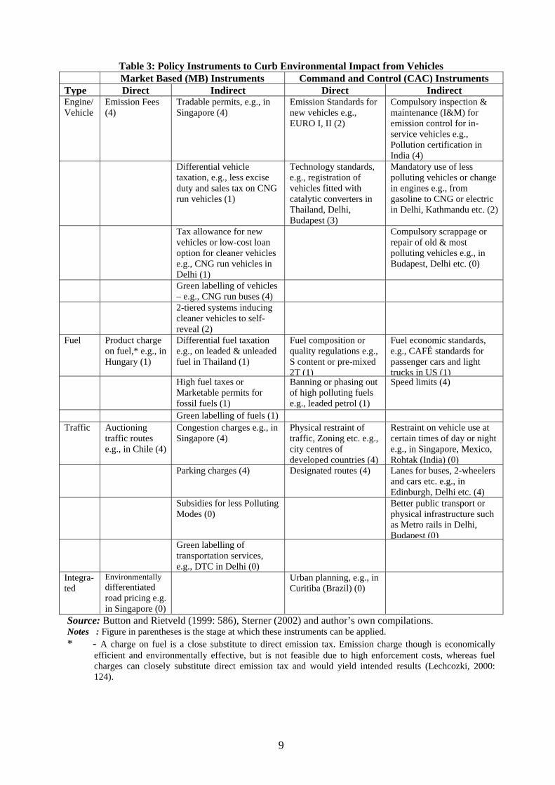
Table 3: Policy Instruments to Curb Environmental Impact from Vehicles Market Based (MB) Instruments Command and Control (CAC) InstrumentsType Direct Indirect Direct IndirectEngine/ Vehicle

Emission Fees (4)

Tradable permits, e.g., in Singapore (4)

Emission Standards for new vehicles e.g., EURO I, II (2)

Compulsory inspection & maintenance (I&M) for emission control for in-service vehicles e.g., Pollution certification in India (4)

Differential vehicle taxation, e.g., less excise duty and sales tax on CNG run vehicles (1)

Technology standards, e.g., registration of vehicles fitted with catalytic converters in Thailand, Delhi, Budapest (3)

Mandatory use of less polluting vehicles or change in engines e.g., from gasoline to CNG or electric in Delhi, Kathmandu etc. (2)

Tax allowance for new vehicles or low-cost loan option for cleaner vehicles e.g., CNG run vehicles in Delhi (1)

Compulsory scrappage or repair of old & most polluting vehicles e.g., in Budapest, Delhi etc. (0)

Green labelling of vehicles – e.g., CNG run buses (4)

2-tiered systems inducing cleaner vehicles to self-reveal (2)

Fuel Product charge on fuel,* e.g., in Hungary (1)

Differential fuel taxation e.g., on leaded & unleaded fuel in Thailand (1)

Fuel composition or quality regulations e.g., S content or pre-mixed 2T (1)

Fuel economic standards, e.g., CAFÉ standards for passenger cars and light trucks in US (1)

High fuel taxes or Marketable permits for fossil fuels (1)

Banning or phasing out of high polluting fuels e.g., leaded petrol (1)

Speed limits (4)

Green labelling of fuels (1) Traffic Auctioning

traffic routes e.g., in Chile (4)

Congestion charges e.g., in Singapore (4)

Physical restraint of traffic, Zoning etc. e.g., city centres of developed countries (4)

Restraint on vehicle use at certain times of day or night e.g., in Singapore, Mexico, Rohtak (India) (0)

Parking charges (4) Designated routes (4) Lanes for buses, 2-wheelers and cars etc. e.g., in Edinburgh, Delhi etc. (4)

Subsidies for less Polluting Modes (0)

Better public transport or physical infrastructure such as Metro rails in Delhi, Budapest (0)

Green labelling of transportation services, e.g., DTC in Delhi (0)

Integra-ted

Environmentally differentiated road pricing e.g. in Singapore (0)

Urban planning, e.g., in Curitiba (Brazil) (0)

Source: Button and Rietveld (1999: 586), Sterner (2002) and author’s own compilations. Notes : Figure in parentheses is the stage at which these instruments can be applied. * - A charge on fuel is a close substitute to direct emission tax. Emission charge though is economically

efficient and environmentally effective, but is not feasible due to high enforcement costs, whereas fuel charges can closely substitute direct emission tax and would yield intended results (Lechcozki, 2000: 124).

9

CORRECTING AN EXTERNALITY – ESTIMATING THE DAMAGE

As mentioned in a distortion free world, an externality can be optimally corrected by imposing

a charge equal to the short-run marginal external or social costs (i.e., imposing a charge

equivalent to Po1–Pa). In reality estimating this short-run marginal costs are extremely difficult.

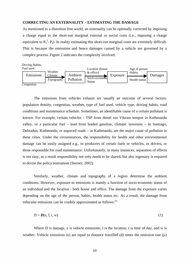
This is because the emissions and hence damages caused by a vehicle are governed by a

complex process. Figure 2 indicates the complexity involved.

Figure 2: Link between emissions to damages

Driving Habits, Fuel used Congestion

Age of person Habits Health status

Location (house & office)

Socio-economic Status

Weather Climate Topography

Ambient Pollution

Exposure DamagesEmissions

The emissions from vehicles exhaust are usually an outcome of several factors:

population density, congestion, weather, type of fuel used, vehicle type, driving habits, road

conditions and maintenance schedule. Sometimes, an identifiable cause of a certain pollutant is

known. For example, certain vehicles - TSP from diesel run Vikram tempos in Kathmandu

valley, or a particular fuel – lead from leaded gasoline, climatic inversion – in Santiago,

Dehradun, Kathmandu, or unpaved roads – in Kathmandu, are the major cause of pollution in

these cities. Under the circumstances, the responsibility for health and other environmental

damage can be easily assigned e.g., to producers of certain fuels or vehicles, or drivers, or

those responsible for road maintenance. Unfortunately, in many instances, separation of effects

is not easy, as a result responsibility not only needs to be shared, but also ingenuity is required

to devise the policy instrument (Sterner, 2002).

Similarly, weather, climate and topography of a region determine the ambient

conditions. However, exposure to emissions is mainly a function of socio-economic status of

an individual and the location - both house and office. The damage from the exposure varies

depending on the age of the person, habits, health status etc. As a result, the damage from

vehicular emissions can be crudely approximated as follows:14

D = D(e, l, t, w) (1)

Where D is damage, e is vehicle emissions, l is the location, t is time of day, and w is

weather. Vehicle emissions (e) are equal to distance travelled (d) times the emission rate (µ)

10

(i.e., e = d*µ). The emission rate µ (= µ(v, f, to, r, z)) is a function of vehicle characteristics (v),

fuel characteristics (f), outside temperature (to), road conditions (r), and a vector of driving

related variables (z = z(s, ad, et, m)) that include speed (s), acceleration and deceleration

patterns (ad), engine temperature (et) and maintenance (m) (Sterner, 2002: 228). The average

speed is again a function of congestion level. Thus,

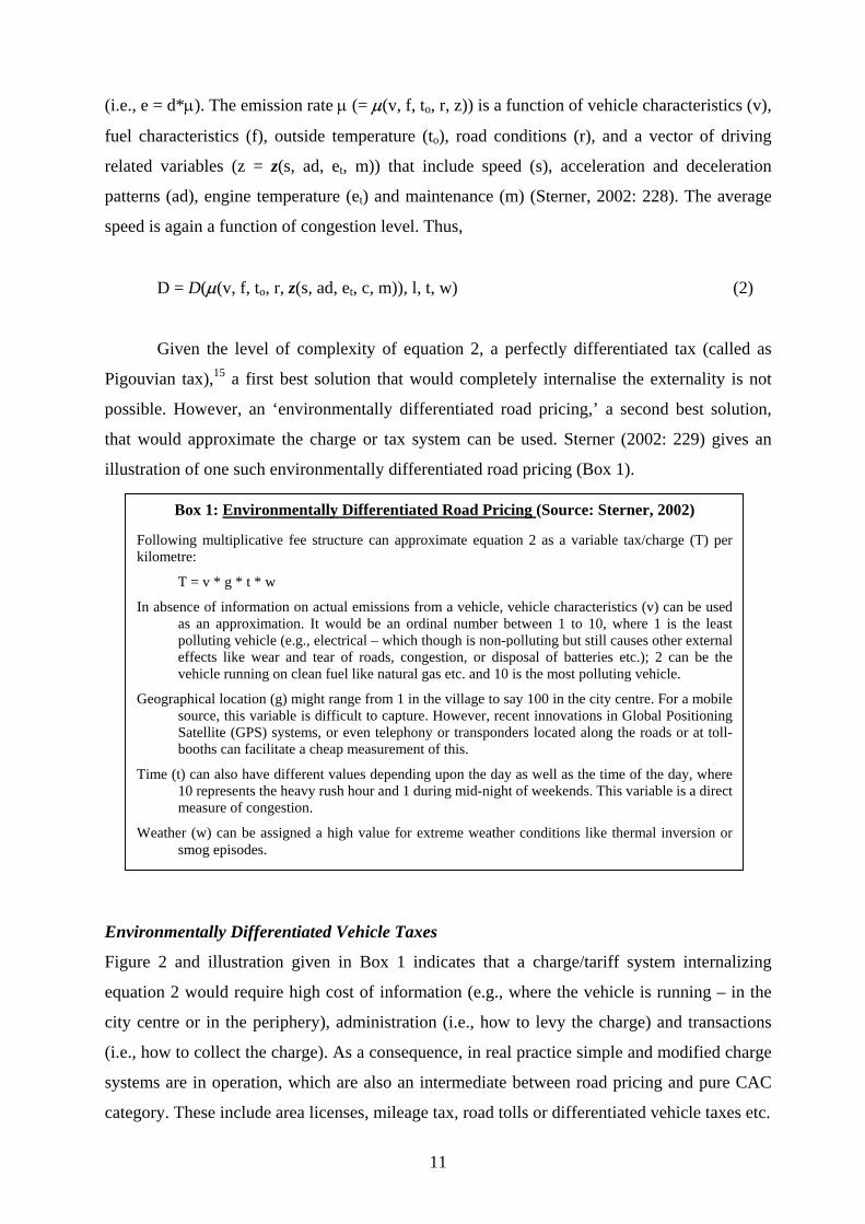
D = D(µ(v, f, to, r, z(s, ad, et, c, m)), l, t, w) (2)

Given the level of complexity of equation 2, a perfectly differentiated tax (called as

Pigouvian tax),15 a first best solution that would completely internalise the externality is not

possible. However, an ‘environmentally differentiated road pricing,’ a second best solution,

that would approximate the charge or tax system can be used. Sterner (2002: 229) gives an

illustration of one such environmentally differentiated road pricing (Box 1).

Box 1: Environmentally Differentiated Road Pricing (Source: Sterner, 2002)

Following multiplicative fee structure can approximate equation 2 as a variable tax/charge (T) perkilometre:

T = v * g * t * w In absence of information on actual emissions from a vehicle, vehicle characteristics (v) can be used

as an approximation. It would be an ordinal number between 1 to 10, where 1 is the leastpolluting vehicle (e.g., electrical – which though is non-polluting but still causes other externaleffects like wear and tear of roads, congestion, or disposal of batteries etc.); 2 can be thevehicle running on clean fuel like natural gas etc. and 10 is the most polluting vehicle.

Geographical location (g) might range from 1 in the village to say 100 in the city centre. For a mobile

source, this variable is difficult to capture. However, recent innovations in Global PositioningSatellite (GPS) systems, or even telephony or transponders located along the roads or at toll-booths can facilitate a cheap measurement of this.

Time (t) can also have different values depending upon the day as well as the time of the day, where

10 represents the heavy rush hour and 1 during mid-night of weekends. This variable is a directmeasure of congestion.

Weather (w) can be assigned a high value for extreme weather conditions like thermal inversion or

smog episodes.

Environmentally Differentiated Vehicle Taxes

Figure 2 and illustration given in Box 1 indicates that a charge/tariff system internalizing

equation 2 would require high cost of information (e.g., where the vehicle is running – in the

city centre or in the periphery), administration (i.e., how to levy the charge) and transactions

(i.e., how to collect the charge). As a consequence, in real practice simple and modified charge

systems are in operation, which are also an intermediate between road pricing and pure CAC

category. These include area licenses, mileage tax, road tolls or differentiated vehicle taxes etc.

11

In Singapore potential car owners are required to purchase a vehicle entitlement at a

monthly auction – an example of area licenses. In Germany, the expressway user charges are

differentiated not only by time but also by exhaust characteristics – as a result trucks or cars

meeting EURO II pay less – an example of mileage taxes. Similarly, in Switzerland, the fee per

unit of load and km driven by heavy vehicles is different depending upon the emission

category in which the truck is falling with the lowest in EURO II and III and highest for EURO

0 compliant trucks (Sterner, 2002). In California (US), Oslo, Trondheim and Bergen (Norway)

and Singapore vehicle owners pay different charges for city centres and on toll roads

depending on the day and time of travel. In many countries differential tax is levied on vehicles

depending on their emission factors. For example, in Sweden from 1986 onwards, cars with

catalytic converters were given tax credits and from 1995 onwards, passenger cars meeting

higher standards were exempt from annual tax on car ownership for five years. A variant of

this has been introduced in Tamil Nadu (India), where from 2004 onwards, vehicles beyond a

certain age have to pay annual tax.

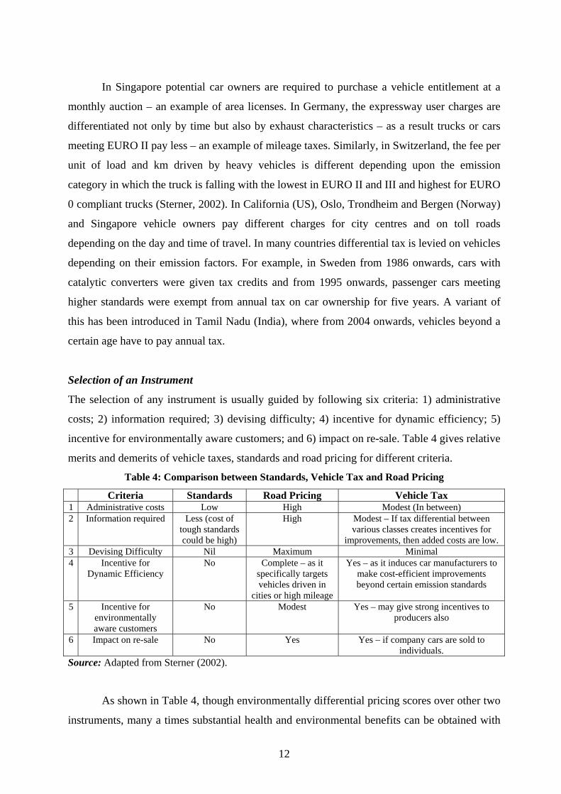
Selection of an Instrument

The selection of any instrument is usually guided by following six criteria: 1) administrative

costs; 2) information required; 3) devising difficulty; 4) incentive for dynamic efficiency; 5)

incentive for environmentally aware customers; and 6) impact on re-sale. Table 4 gives relative

merits and demerits of vehicle taxes, standards and road pricing for different criteria.

Table 4: Comparison between Standards, Vehicle Tax and Road Pricing

Criteria Standards Road Pricing Vehicle Tax 1 Administrative costs Low High Modest (In between) 2 Information required Less (cost of

tough standards could be high)

High Modest – If tax differential between various classes creates incentives for

improvements, then added costs are low. 3 Devising Difficulty Nil Maximum Minimal 4 Incentive for

Dynamic Efficiency No Complete – as it

specifically targets vehicles driven in

cities or high mileage

Yes – as it induces car manufacturers to make cost-efficient improvements beyond certain emission standards

5 Incentive for environmentally aware customers

No Modest Yes – may give strong incentives to producers also

6 Impact on re-sale No Yes Yes – if company cars are sold to individuals.

S

ource: Adapted from Sterner (2002).

As shown in Table 4, though environmentally differential pricing scores over other two

instruments, many a times substantial health and environmental benefits can be obtained with

12

simple regulatory and administrative measures such as zoning, retiring the most polluted

vehicles, paving roads, phasing out leaded gasoline, restoring public transport, managing

traffic or investing in driver education. The situations in which regulatory measures are

warranted include protection of schools, hospitals and residential areas from excessive level of

pollution and night-time noise or a situation involving emissions during cold start, where the

emissions increase manifold due to cold catalyst. In the later case, making electric motor

heaters mandatory and providing the necessary electricity at parking meters will reap more

benefits (Sterner, 2002: 237).

SELECTING POLICY INSTRUMENTS TO CURB POLLUTION IN MEGA CITIES AND INDIA’S EXPERIENCE The choice and selection of policy instruments to curb pollution in mega cities can be dictated

by three main objectives: a) fewer vehicle kilometres to be travelled; b) less fuel used per

kilometre travelled; and c) less emission per unit of fuel used (World Bank, 2001a: 3). The first

objective i.e., aiming to reduce vehicle kilometres can be realised by means such as, giving

priority to public transport through special lanes, parking provisions etc.; discouraging private

transport through high congestion parking, adopting day-of-the-week strategy etc. The second

objective, where the aim is that less fuel is consumed for each kilometre travelled can be

actualised by introducing fuel economy standards, inducing lane driving or by installing timers

at different intersections. The fulfilment of third objective requires improvement in fuel

characteristics, engine specification, shift from polluting fuel to clean fuel etc.

For each objective, there exists three categories of instruments – technological

(requiring technical solution to the pollution problem); administrative (primarily regulation

based); and economic or MB instruments (using market mechanism to change the behaviour).

Table 5 gives a synoptic view of different categories of instruments for each objective.

Depending on the objective in mind, the policy makers can choose a policy instrument.

India’s Experience in Combating Vehicular Air Pollution

The vehicular pollution problem in the urban areas of the country can be characterised by the

following: a) high vehicle density; b) vehicle vintage dominated by older vehicles; c)

heterogeneous traffic mix; d) inadequate I&M facilities; e) predominance of 2-stroke 2-

wheelers; f) adulteration of fuel; g) improper traffic management; h) poor road conditions; i)

high levels of pollution at traffic intersections; j) absence of effective MRTS; and k) various

encumbrances on road such as encroachments, unauthorised construction particularly of

13

religious nature. A high level of urban air pollution with vehicles contributing the most has

resulted in implementation of a number of policy instruments in the country. Table 6 gives a

synoptic view of different categories of instruments implemented for Delhi and other cities.

Since most of the policy instruments – whether it is banning of registration of 2-stroke

engines or switching to CNG by public transport or timers at intersections or lanes for HOVs

etc. – have been implemented in Delhi, it will be interesting to see the impact of these

instruments on the pollution profile. Table 7 gives the average value in the past 5 years for

different pollution parameters at Bahadur Shah Zafar Marg, one of the busiest intersections in

Delhi. The table also compares the average values with the prescribed standards.

14

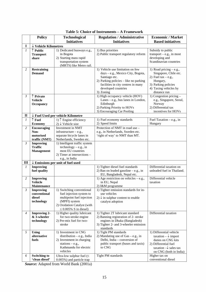
Table 5: Choice of Instruments – A Framework Policy Technological

Initiatives Regulation / Administrative

Initiatives Economic / Market

Based initiatives I ↓ Vehicle Kilometres 1 ↑ Public

Transport share

1) Dedicated busways e.g., in Bogota

2) Starting mass rapid transportation system (MRTS) like Metro rail.

1) Bus priorities 2) Public transport regulatory reform

Subsidy to public transport – e.g., in most developing and Scandinavian countries

2 Restraining Demand

1) Vehicle use limitation on few days – e.g., Mexico City, Bogota, Santiago etc.

2) Parking policies – like no parking facilities in city centres in many developed countries

3) Zoning

1) Road pricing – e.g., Singapore, Chile etc.

2) Fuel tax – e.g., Hungary,

3) Parking policies 4) Taxing vehicles by

distance run 3 ↑ Private

Vehicle Occupancy

1) High occupancy vehicle (HOV) Lanes – e.g., bus lanes in London, Edinburgh

2) Parking Priority to HOVs 3) Encouraging Car Pooling

1) Congestion pricing – e.g., Singapore, Seoul, Norway

2) Differential tax incentives for HOVs

II ↓ Fuel Used per vehicle Kilometre 1 ↑ Fuel

Economy 1) ↑ Engine efficiency 2) ↓ Vehicle size

1) Fuel economy standards 2) Speed limits

Fuel Taxation – e.g., in Hungary

2 Encouraging Non-motorised traffic (NMT)

Investment in NMT infrastructure – e.g., separate bicycle lanes in Netherlands, Sweden etc.

Protection of NMT in road use – e.g., in Netherlands, Sweden etc. ‘right of way’ to NMT than MT.

3 Improving Traffic Management

1) Intelligent traffic system technology – e.g., in most EU countries

2) Timer at intersections – e.g., in India

III ↓ Emissions per unit of fuel used 1 Improving

fuel quality 1) Tighter diesel fuel standards

2) Ban on leaded gasoline – e.g., in EU, Bangladesh, Nepal etc.

Differential taxation on unleaded fuel in Thailand.

2 Improving Vehicle Maintenance

1) Age restriction on vehicles – e.g., in EU, Nepal

2) I&M programme

Differential vehicle taxation

3 Improving conventional diesel technology

1) Switching conventional fuel injection system to multipoint fuel injection (MPFI) system

2) Oxidation Catalyst (with ≤ 0.005% S in diesel)

1) Tighter emission standards for in-use vehicles

2) ↓ in sulphur content to enable catalyst adoption

4 Improving 2- & 3-wheeler technology

1) Higher quality lubricant for two-stroke engine

2) Pre-mix fuel for two-stroke

1) Tighter 2T lubricant standard 2) Banning registration of 2- stroke

engines in Dhaka (Bangladesh) 3) Tighter 2- and 3-wheeler emission

standards

Differential taxation

5 Using alternative fuels

1) Investment in CNG distribution – e.g., India

2) Investment in charging stations – e.g., Kathmandu for electric vehicles

1) Tight PM standards 2) Mandating use of Gas – e.g., in

Delhi, India – conversion of public transport (buses and taxis) to CNG

1) Differential vehicle taxation – ↓ import duties on CNG kits

2) Differential fuel taxation –↓ sales tax on CNG (both in India)

6 Switching to ‘clean diesel’

Ultra-low sulphur fuel (≤ 0.005%) and particle trap

Tight PM standards Higher tax on conventional diesel

Source: Adapted from World Bank (2001a)

15

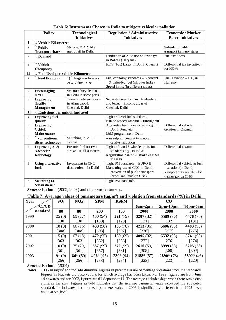
Table 6: Instruments Chosen in India to mitigate vehicular pollution Policy Technological

Initiatives Regulation / Administrative

Initiatives Economic / Market

Based initiatives I ↓ Vehicle Kilometres 1 ↑ Public

Transport share Starting MRTS like metro rail in Delhi

Subsidy to public transport in many states

2 ↓ Demand Limitation of Auto use on few days in Rohtak (Haryana).

Fuel tax / cess

3 ↑ Vehicle Occupancy

HOV (bus) Lanes in Delhi, Chennai Differential tax incentives for HOVs

II ↓ Fuel Used per vehicle Kilometre 1 ↑ Fuel Economy 1) ↑ Engine efficiency

2) ↓ Vehicle size Fuel economy standards – S content

& unleaded fuel (all over India) Speed limits (in different cities)

Fuel Taxation – e.g., in Hungary

2 Encouraging NMT

Separate bicycle lanes in Delhi in some parts.

3 Improving Traffic Management

Timer at intersections – in Ahmedabad, Chennai, Delhi

Separate lanes for cars, 2-wheelers and buses – in some areas of Chennai, Delhi

III ↓ Emissions per unit of fuel used 1 Improving fuel

quality Tighter diesel fuel standards

Ban on leaded gasoline – throughout

2 Improving Vehicle Maintenance

Age restriction on vehicles – e.g., in Delhi, Pune etc.

I&M programme in Delhi

Differential vehicle taxation in Chennai

3 ↑ conventional diesel technology

Switching to MPFI system

↓ in sulphur content to enable catalyst adoption

4 Improving 2- & 3-wheeler technology

Pre-mix fuel for two-stroke - in all 4 metros

Tighter 2- and 3-wheeler emission standards e.g., in India

Registration ban of 2- stroke engines in Delhi

Differential taxation

5 Using alternative fuels

Investment in CNG distribution – in Delhi

Tight PM standards – EURO II Mandating use of CNG in Delhi –

conversion of public transport (buses and taxis) to CNG

Differential vehicle & fuel taxation (in Delhi) –

↓ import duty on CNG kit ↓ sales tax on CNG

6 Switching to ‘clean diesel’

Tight PM standards

Source: Kathuria (2002, 2004) and other varied sources. Table 7: Average values of parameters (µg/m3) and violation from standards (%) in Delhi

CO SO2 NOx SPM RSPM 6am-2pm 2pm-10pm 10pm-6am

Year CPCB

standard 80 80 200 100 2000 2000 2000 1999 25 (0)

[130] 69 (27) [130]

430 (94) [130]

221 (79) [128]

3287 (82) [131]

5589 (96) [132]

4478 (76) [131]

2000 18 (0) [308]

60 (16) [308]

438 (96) [308]

185 (78) [307]

4213 (96) [276]

5606 (98) [277]

4483 (95) [275]

2001 15 (0) [363]

67 (18) [363]

472 (95) [362]

180 (69) [358]

4095 (82) [272]

6532 (93) [276]

5741 (98) [274]

2002 10 (0) [361]

75 (29) [361]

537 (99) [357]

272 (99) [361]

2616 (59) [308]

3999 (83) [308]

3205 (58) [302]

2003 9* (0) [256]

86* (59) [256]

496* (97) [253]

230* (94) [254]

2188* (57) [223]

2890* (73) [223]

2392* (46) [220]

Source: Kathuria (2004) Notes: CO - in mg/m3 and for 8-hr duration. Figures in parenthesis are percentage violations from the standards.

Figures in brackets are observations for which average has been taken. For 1999, figures are from June 14 onwards and for 2003, figures are till September 14. The average excludes days when there was a dust storm in the area. Figures in bold indicates that the average parameter value exceeded the stipulated standard. * - indicates that the mean parameter value in 2003 is significantly different from 2002 mean value at 5% level.

16

It can be seen from Table 7 that barring SO2 all other parameters still exceed the standards by a wide margin. The switching of public transport to CNG on December 2002 has resulted in fall in CO value, whereas the NOx value is on the rise. Surprisingly there is not much decline in SPM and PM10 levels, though one can argue that in absence of policy measures, the values could have been much higher. CONCLUDING REMARKS AND POLICY IMPLICATIONS

This note gives in brief the causes of air pollution in cities and what options do we have to curb the menace. The note also gives a synoptic view of different instruments applied in a number of developing and developed countries. From the instruments employed, it is evident that most developing countries including India have relied primarily on air pollution related regulatory instruments. Recently, in many countries policy makers have initiated a shift from dedicated fuel efficiency and atmospheric pollution regulation to pure transport policies like road pricing, parking and collective transport. The shift has multi-facet benefit as it addresses both the pure transport related externalities like congestion, traffic accidents etc., and has a large beneficial impact on air pollution. Unfortunately, most of the South Asian and other developing countries have not yet resorted to such policies and they still consider the two problems separable.

Given the fact that many developing countries cities are experiencing volcanic growth of vehicular population,16 policy makers need to move away from pure air pollution related measures to transport related instruments, if they want to control pollution. Such a move would take care of pollution from in-service vehicles too, which contribute significantly to the pollution load. The studies indicate that for Indian conditions 20% of bad in-service vehicles contribute as much as 60% of total vehicular emissions (Pundir, 2001).

In fact, the containment of vehicular pollution requires an integrated approach, with

following components: (i) improvement of public transport system; (ii) optimisation of traffic and improvement in traffic management17 (e.g., area traffic control system, timers at intersection, no-traffic zone, green corridors, removal of encroachment on roads, regulation of digging of roads); (iii) comprehensive inspection and certification system for on-road vehicles; (iv) phasing out of grossly polluting units; (v) fuel quality improvement (e.g., benzene and aromatics in petrol, reduction of sulphur in diesel); (vi) tightening of emission norms (e.g., EURO-IV); (vii) improvement in vehicle technology (e.g., restriction on manufacturing of 2-stroke engines, emission warranty, on-board diagnostic system); (viii) checking fuel adulteration; and (ix) checking evaporative emissions from storage tanks and fuel distribution system.

17

REFERENCES Blackman, A. and Harrington, W. (2000) The use of economic incentives in developing

countries: Lessons from international experience with industrial air pollution. The Journal of Environment and Development 9, 5-44.

Button, K.J. and Rietveld, P. (1999) Transport and the environment. In Handbook of Environmental and Resource Economics, ed. J.C.J.M. van den Bergh, pp. 581-89. Edward Elgar, Cheltenham.

Central Pollution Control Board (1999) Parivesh: Newsletter, 6(1), June, CPCB, Ministry of Environment and Forests, Delhi.

Cropper, M.L., Simon, N.B., Alberini, A., Arora, S. and Sharma, P.K. (1997) The health benefits of air pollution control in Delhi. American Journal of Agricultural Economics 79, 1625-29.

da Motta, R.S. and Behrem, M.R. (2000) Air pollution tradable permits in Santiago, Chile. In Economic Instruments for Environmental Management, eds J. Rietbergen-McCracekn and H. Abaza, pp. 178-84. Earthscan, London.

Faiz, A., C.S. Weaver, and M.P. Walsh (1996) Air Pollution from Motor Vehicles, International Bank for Reconstruction and Development/World Bank.

Frailey, M., Norton, P., Clark, N. N., Lyons, D.W. (2000) An evaluation of natural gas versus diesel in medium duty buses, SAE Technical Paper Series 2000-01-2822, Warrendale, Pennsylvania.

Johansson, O. (1997) “Optimal Road Pricing: Simultaneous Treatment of Time Losses, Increased fuel consumption, and Emissions”, Transportation Research – Part D, Vol. 2(2), 77-87.

Kathuria, V. (2004) “Impact of CNG on Vehicular Pollution in Delhi – a note”, Transportation Research – Part D, 9 (5): 409-17.

Kathuria, V. (2002) “Vehicular Pollution Control in Delhi, India”, Transportation Research – Part D, 7(5): 373-87.

Krawack, S. (1993) “Traffic Management and Emissions”, The Science of the Total Environment, 134: 305-14.

Lehoczki, Z. (2000) Product charge on transport fuel in Hungary. In Economic Instruments for Environmental Management, eds J. Rietbergen-McCracekn and H. Abaza, pp. 122-34. Earthscan, London.

Nylund, N.O., Lawson, A. (2000) Exhaust emissions from natural gas vehicles. International Association of natural gas Vehicles, VTT Energy, Finland.

Pundir, B.P. (2001), ‘Vehicular Air Pollution in India: Recent Control Measures and Related Issues’, in India Infrastructure Report 2001, Oxford University Press, Delhi.

18

Sterner, T. (2002), The Selection and Design of Policy Instruments: Applications to Environmental Protection and Natural Resource Management, Resources for Future and the World Bank.

Watt, G.M. (2001) Natural gas vehicle transit bus fleets: The current international experience. IANGV review paper, available <http:/www.iangv.org/html/sources/reports/iangv_bus_report.pdf >.

World Bank (2001a) Vehicular air pollution: setting priorities, South Asian Urban Air Quality Management Briefing Note No. 1, ESMAP, World Bank.

World Bank (2001b) International experience with CNG vehicles, South Asian Urban Air Quality Management Briefing Note No. 1, ESMAP, World Bank.

19

Foot Note

1 The use of data pertaining to total pollutants emitted in tons per year need to be interpreted with caution. This

is because it ignores the varying toxicity of different pollutants, often leading to erroneous conclusion that transport is the major polluter (World Bank, 2001a). Still, it is a useful indicator.

2 Source: www.oneworld.org/cse/html/eyou/eyou222.htm accessed in June 2001. 3 Source: ibid. 4 Source: Faiz, Weaver and Walsh, 1996 as referred in Sterner (2002). 5 In the US since 1999, the measurement of TSP has yielded to that of PM10 and PM2.5. In Kathmandu valley

too, since 2002 instead of measuring TSP, monitoring stations are measuring PM2.5. 6 Highways or large roads when cut through a village or community or a small town create barriers to

communication and movement of both animals and humans. This makes it often difficult for people to socialize, shop or work on the other side of the road. This is called as ‘barrier effect’.

7 A part of this and next section is taken from Kathuria (2002 and 2004). 8 The Reid vapor pressure (RVP) means the absolute vapor pressure of a petroleum product in pounds per

square inch (or kilopascals) at 100 degrees Fahrenheit (37.8 degrees Celsius). 9 The cetane number measures the ignition quality of a diesel fuel. A high cetane number indicates greater fuel

efficiency. 10 Liquefied natural gas (LNG) is another fuel substitute to diesel (and gasoline). However, of the 1.74 million

vehicles running on natural gas, majority are CNG vehicles (World Bank, 2001b: 1). 11 As referred in Johansson (1997). 12 In fact, the effectiveness of tax on gasoline or diesel in controlling pollution is limited due to the price

inelasticity of demand. Still the proceeds can be used to cleanup the environment as in the case of Hungary or for developing road network as in India.

13 Refer Kathuria (2002, 2004) for a list and role of different instruments implemented in Delhi. 14 The remaining section follows from Sterner (2002: 228-40). 15 Pigou was the first person to suggest levying of taxes on polluters as a corrective mechanism for negative

externality. 16 For example, the daily registration in Delhi varies between 370-600. This implies approximately 150,000 to

200,000 new vehicles are added every year (Kathuria, 2002). 17 An earlier study by Central Road Research Institute (CRRI) found that in 1996, 321 kilolitres (KL) of petrol

and 101 KL of diesel was wasted everyday at 466 intersections in Delhi. Thus, causing an annual loss of about Rs. 2,450 million at 1996 prices (Source: Hindustan Times, 14.1.1999). A simple solution that would minimise this loss is by proper synchronization of traffic signals.

Please send your comments to the author at vinish@mse.ac.in

20