Modeling energy consumption and CO2 emissions at the urban ...

Modeling energy consumption and CO2 emissions at the urban scale:Methodological challenges and insights from the United States

Lily Parshall a,!, Kevin Gurney b, Stephen A. Hammer a, Daniel Mendoza b,Yuyu Zhou b, Sarath Geethakumar b

a Center for Energy, Marine Transportation and Public Policy, Columbia University, 514 West 113th Street, New York, NY 10025, United Statesb Department of Atmospheric Sciences, 550 West Stadium Mall Drive, Purdue University, West Lafayette, IN 77907, United States

a r t i c l e i n f o

Article history:Received 23 March 2009Accepted 14 July 2009

Keywords:Urban energyEmissions inventoryUnited states

a b s t r a c t

Local policy makers could benefit from a national, high-resolution inventory of energy consumption andrelated carbon dioxide (CO2) emissions based on the Vulcan data product, which plots emissions on a100 km2 grid. We evaluate the ability of Vulcan to measure energy consumption in urban areas, a scaleof analysis required to support goals established as part of local energy, climate or sustainabilityinitiatives. We highlight the methodological challenges of this type of analytical exercise and reviewalternative approaches. We find that between 37% and 86% of direct fuel consumption in buildings andindustry and between 37% and 77% of on-road gasoline and diesel consumption occurs in urban areas,depending on how these areas are defined. We suggest that a county-based definition of urban ispreferable to other common definitions since counties are the smallest political unit for which energydata are collected. Urban counties, account for 37% of direct energy consumption, or 50% if mixed urbancounties are included. A county-based definition can also improve estimates of per-capita consumption.

& 2009 Elsevier Ltd. All rights reserved.

1. Introduction

While federal and state governments dictate much of USenergy policy, increasingly municipal authorities are engaging onenergy issues, often within the context of local climate orsustainability initiatives. Because of their density of demand,cities can take advantage of a wide array of technology and policyoptions to increase energy efficiency and reduce per-capitaconsumption of fossil fuels. But local planners also face severalchallenges, including inadequate data, decentralized energyplanning, and the difficulty of formulating local policy to addressnational and international problems.

In this paper we suggest that local policy makers could benefitfrom a national, high-resolution inventory of energy consumptionand related carbon dioxide (CO2) emissions. A national inventory,completed at regular intervals, would allow local authorities toestablish baseline energy consumption and monitor changes overtime, compare themselves to other similar localities, set appro-priate energy- and emissions-reduction targets, and support localparticipation in carbon markets. Such an inventory also couldprovide the type of consistent data needed to analyze howdifferent aspects of the urban environment interact with socio-

demographic factors to shape patterns of energy use, informingdebates on smart growth and urban sprawl.

The Vulcan data product is promising as the basis of aninventory because it consolidates data from a wide variety ofpoint, non-point, and mobile sources and quantifies these data intheir ‘‘native’’ resolution (geocoded points, roads, counties) and ona regular 100 km2 (10 km!10km) grid over the conterminousUnited States every hour of the year (Gurney et al., 2008, 2009).Vulcan draws on point source and county-scale non-point sourcedata, the highest resolution at which these data are available.Vulcan was originally conceived of as an inventory of fossil-basedsources of carbon with scientific applications in carbon cyclemodeling, so the results do not cover renewable energy or nuclearpower, which together comprise approximately 28% of electricitysupply. With these exceptions, Vulcan offers complete andsystematic coverage of energy-related CO2 emissions in theresidential, commercial, industrial, transportation, and electricitysectors.1 Since Vulcan categorizes emissions into 50 different sub-fuels, it is relatively straightforward to convert between metrictons of CO2 and gigajoules (GJ) of energy.2 The ability to

ARTICLE IN PRESS

Contents lists available at ScienceDirect

journal homepage: www.elsevier.com/locate/enpol

Energy Policy

0301-4215/$ - see front matter & 2009 Elsevier Ltd. All rights reserved.doi:10.1016/j.enpol.2009.07.006

! Corresponding author. Tel.: +12128540615; fax: +12128540603.E-mail address: [email protected] (L. Parshall).

1 Vulcan also covers carbon emissions associated with agriculture and cementproduction.

2 For clarity, we refer to the detailed fuel breakdown, which distinguishesbetween different types of coal (e.g. bituminous vs. subbituminous), natural gas(e.g. gas vs. LPG), and fuel oil (e.g. distillate vs. residual), as ‘‘sub-fuel’’ data.

Please cite this article as: Parshall, L., et al., Modeling energy consumption and CO2 emissions at the urban scale: Methodologicalchallenges and insights from the United States. Energy Policy (2009), doi:10.1016/j.enpol.2009.07.006

Energy Policy ] (]]]]) ]]]–]]]

mailto:[email protected]

ARTICLE IN PRESS

distinguish between the energy and carbon intensity of differentsectors can help local authorities analyze trade-offs betweenpolicies to reduce energy consumption and policies to reduce thecarbon intensity of fuel use.

Much of the literature on local energy consumption andemissions inventories focuses on urban areas. Interest in urbanenergy consumption stems from the central role that cities play inshaping global energy demand as well as growing urban leader-ship on climate change mitigation. Our research began as part ofan effort by the International Energy Agency (IEA) to quantifyurban energy consumption for the 2008 World Energy Outlook(WEO) (IEA, 2008). The IEA study found that globally, urban areasaccount for 67% of energy consumption and 71% of CO2 emissionsworldwide, figures that are expected to rise in the coming decadesgiven global demographic trends (IEA, 2008).

We used Vulcan to estimate US urban energy consumption forthe IEA study since Vulcan is the only national dataset withsufficient spatial resolution to isolate urban and rural areas.We found that 80% of the United States’ energy consumptionoccurs in urban areas, which have slightly lower per-capitaconsumption than the nation as a whole (IEA, 2008).3 Weused the United Nations’ (UN) definition of urban for the UnitedStates to maintain consistency with estimates for other regionscovered by the IEA analysis (UN, 2009). However, as we showin this paper, the share of energy consumption attributed tourban areas varies widely depending on how urban areas aredefined and bounded in space. We suggest that efforts tocreate local inventories should be mindful of how differentspatial scales and urban thresholds affect perceived patterns ofurban and rural energy consumption. Inventories that canproperly distinguish between localities of different character areneeded to make meaningful comparisons of per-capita energyconsumption and the energy intensity of different local economiesand lifestyles.

A national inventory of local-scale energy use requires the typeof data provided by Vulcan at a spatial resolution appropriate forlocal energy governance. Through our analysis of US urban energyconsumption, we combine an exploration of different urban/ruralclassification systems with an evaluation of Vulcan’s currentability to measure local energy use. We highlight methodologicalchallenges inherent in this type of analytical exercise and reviewalternative approaches. We conclude by recommending improve-ments in future energy and CO2 emissions inventories, which willhelp policy makers at multiple scales make informed decisionsregarding energy supply and demand, fossil fuel consumption,and climate change mitigation.

2. Estimating energy consumption and CO2 emissions atsmall spatial scales

Currently, there is no centralized reporting of local energyconsumption, or related CO2 emissions, in the United States.4 Agrowing number of studies are developing their own estimates atsmall spatial scales. These studies fall into two broad categories:(1) those that inventory local emissions to directly support localpolicy objectives and (2) those that analyze a cross-section

of localities to derive general relationships between energy useand patterns of urban development. Both types of studiesaddress the dearth of local energy statistics by culling data frommultiple sources. They use a combination of downscaling,aggregation, and weighting to estimate consumption at the scaleof interest (e.g. metropolitan areas, urban areas, cities, towns, orcounties).

ICLEI–Local Governments for Sustainability was one of the firstorganizations to help local governments conduct GHG emissionsinventories.5 Local authorities prepare two types of inventories:(1) a ‘‘corporate’’ inventory of emissions associated with govern-ment buildings, streetlights, traffic signals, and the city-operatedvehicle fleet (‘‘organizational boundary’’)6; and (2) a city-wide ‘‘community’’ inventory that covers the residential, com-mercial, industrial, transportation, and waste sectors (‘‘geopoli-tical boundary’’).7 For energy-related CO2 emissions, ICLEI hashistorically focused on accounting for all emissions associatedwith total final consumption (direct fuel consumption andelectricity demand) within a geopolitical boundary. ICLEI hasstandardized the inventory process by commissioning a proprie-tary software package and developing the ‘‘International LocalGovernment GHG Emissions Analysis Protocol’’ (ICLEI, 2008b), butcities complete the inventories themselves; have some latitude intheir choice of data, baseline year, and level of detail; and are freeto decide whether and how to disseminate inventory data andresults.8

Whereas ICLEI’s main objective is to support the emissionsreduction efforts of local governments, cross-sectional studiesseek to provide an analytical underpinning for sustainabledevelopment goals such as reducing urban sprawl and promotingpublic transportation. The majority of cross-sectional studiesdevelop regression models that relate energy consumption tophysical, economic, and social aspects of the urban environment.The dependent variable in these models is typically an energy oremissions indicator such as total or per-capita consumption for aparticular fuel or sector. Independent variables to be tested orcontrolled for might include climate, population density, housingcharacteristics, energy prices, commuting distance, various in-dicators of sprawl, and various economic indicators such as GDP,industry mix, or per-capita income. These exercises often usehousehold surveys or other types of sample data rather thancommunity-wide inventories. Examples of residential-sectorstudies include Moyers et al. (2005) and Ewing and Rong(2008)9; examples of transportation-sector studies include Naesset al. (1996) and Holden and Norland (2005).10 Some of these

3 The IEA methodology for computing US urban energy consumption isavailable on the WEO website. The Vulcan data product was used in the USanalysis, but the methodology was somewhat different from the methodologydescribed in this paper (IEA, 2008).

4 We focus on energy-related CO2 emissions, rather than total GHG emissions.Most urban GHG emissions are associated with the combustion of fossil fuels. Inthe United States, energy-related CO2 emissions account for 82% of total GHGemissions (US DOE, 2008a).

5 Local authorities, with technical assistance from ICLEI’s Cities for ClimateChange Program (CCP), complete an inventory as part of a program that includessetting emissions reduction targets, identifying policy measures, and evaluatingprogress. More than 800 local governments worldwide have participated in CCP,many of which have completed GHG emissions inventories (ICLEI, 2008a).

6 CCP corporate inventories, which typically involve analysis of individualutility bills and fuel purchases, provide a detailed accounting, often at the scale ofindividual buildings or government departments.

7 Community inventories incorporate local data on electricity and fuelconsumption when available, but can also be constructed by combining localCensus data with state and regional electricity and fuel consumption indicatorsavailable from the Energy Information Administration (EIA). In the waste sector,the primary source of GHG emissions is methane from landfills.

8 ICLEI (2008b) contains protocols for conducting local inventories, with theintention of providing an internationally recognized set of standards comparableto standards for national inventories developed by the International Panel onClimate Change (IPCC) (ICLEI, 2008b). The document offers a careful treatment ofboundary issues and energy accounting for local-scale inventories.

9 Ewing and Rong used data from the EIA’s Residential Energy ConsumptionSurvey (RECS). See US DOE (2005). Critiques of Ewing and Rong (2008) can befound in Staley (2008) and Randolph (2008).

10 Schipper (1995) reviews the literature on automobile use and energyconsumption in OECD countries.

L. Parshall et al. / Energy Policy ] (]]]]) ]]]–]]]2


ARTICLE IN PRESS

studies offer nuanced findings. For example, Moyers et al. (2005)found that high-rise buildings in Sydney have higher per-capitaCO2 emissions compared with detached dwellings due to smallerhousehold size. Bento et al. (2005), who found that householdcharacteristics have a stronger influence on commute-modechoice than urban-scale characteristics, do not directly analyzeenergy consumption, but their study is a good example of a carefulstatistical analysis.

Several recent studies have combined elements of bothapproaches to develop cross-sectional local inventories. Thesestudies first derive a set of energy indicators and then scale up tothe geographic extent of interest. Although such studies arephilosophically rooted in the cross-sectional approach, theirmethods are similar to the ICLEI community inventories. Oneexample is a recent Brookings study on energy consumption andCO2 emissions in the 100 largest metropolitan areas in the UnitedStates (Brown et al., 2008). The authors compiled residential andhighway transportation data for each metropolitan area for 2000and 2005, constructing a panel that could be used to analyzevariation in time and space.11 Their methodology and data wereconsistent across all metropolitan areas, allowing them to rankand compare the areas and identify broad patterns of final energyconsumption and associated emissions across the most heavilypopulated parts of the country.

The choice of metropolitan areas as a scale of analysis hasseveral implications. An advantage is the availability of detailedGDP data for each metropolitan area, which can be used tobenchmark the energy and carbon intensity of local economies.12

A disadvantage is that metropolitan areas do not explicitlyseparate urban and rural areas. In fact, the majority of the USrural population lives within metropolitan areas (Isserman, 2005).One study addressed this problem by dividing each metropolitanarea into a central city and suburban regions to examine therelationship between urban form and CO2 emissions within, aswell as across, metropolitan areas (Glaeser and Kahn, 2008).13 Likethe Brookings study, Glaeser and Kahn (2008) developed theirown estimates of residential and personal transportation CO2

emissions for a subset of metropolitan areas, but they useddifferent datasets: the 2001 National Household Travel Survey(NHTS) instead of the Highway Performance Monitoring System(HPMS) for transportation and the 2000 Individual Public UseMicrosample (IPUM) instead of US Department of Energy (DOE)data for the residential sector.14 The lack of standardized datasets

is one of many challenges involved in creating inventories that canmeet the needs of those interested in cross-sectional analysis.Often, dependent variables are constructed from multiple datasources and incorporate factors, such as housing characteristics,that intuitively belong as independent factors in statisticalmodels. Metropolitan-scale data also may bear little relevanceto energy use targeted by local energy policy planning, as thepolicy control powers of local authorities tend to end at theirpolitical boundaries, representing a fraction of the geographic areaencompassed by the metropolitan area designation.

2.1. Local energy accounting

Local inventories make implicit assumptions about theboundaries of the local energy sector. In local energy accountinga number of different types of inventories have been recognized:(1) corporate energy use by municipal governments or otherorganizations (e.g. ICLEI corporate inventory); (2) direct finalconsumption within the local territory, where direct fuel con-sumption is included, but the power sector is not15; (3) total finalconsumption within the local territory, including imported energysuch as heat and electricity generated outside an urban area butexcluding energy lost during generation, transmission, anddistribution; (4) total primary energy supply to meet demand inthe local territory including total fuel consumption associatedwith electricity generation; and (5) energy embodied in infra-structure as well as material goods and services. The last categoryencompasses a continuum that spans from life-cycle analysis oflocal infrastructure to a complete footprint of all goods andservices entering and leaving the local territory.

Most local inventories are situated in the third category,suggesting that energy-related CO2 emissions should be attrib-uted to the point of demand rather than to the point ofproduction. This approach is consistent with national energyinventories, which usually cover total final consumption andprimary energy supply. But, national CO2 emissions inventoriesuse production-based accounting so power-sector emissions, forexample, are attributed to the location where they are emitted.From an energy sector perspective, this means that the portion ofCO2 emissions accounts that cover direct final consumption aregenerally consistent with energy accounts, but other portionsare not.

Satterthwaite (2008) discusses the implications of allocatingresponsibility for local sources of CO2 emissions under differentaccounting frameworks. Along with power generation, produc-tion-driven accounts may be inflated by industrial emissionsassociated with products exported from the urban area andtransport emissions associated with through-travel. Satterthwaitesuggests that demand-driven accounting best captures the role ofmiddle- and upper-income groups in driving consumptionpatterns, particularly when the embodied energy of goods andservices is included (Satterthwaite, 2008). Local accounts thatinclude embodied energy fall within the general framework ofecological footprint analysis, which looks at the impact of alocality’s demand on global environmental resources. Estimatingembodied energy demand for a local territory in this way is atime- and data-intensive endeavor, but can help cities andconsumers understand their role in global supply and demandnetworks and associated implications for sustainable develop-ment.16 Quantifying embodied emissions is difficult, particularly

11 The Brookings study chose to focus on these sectors due to datashortcomings (Brown et al., 2008). To estimate residential fuel consumption,Brookings used a similar approach to ICLEI, but relied solely on the EnergyInformation Administration’s (EIA) state data to derive energy indicators fordifferent types of housing stock in different locations rather than incorporateavailable local data. Brown et al. (2008) provides a brief summary of the study’smethodology, data sources, and data gaps. To estimate highway consumption,Brookings used highway traffic count data from the Highway PerformanceMonitoring System (HPMS) to estimate VMT and associated fuel consumption(Brown et al., 2008). Brown and Logan (2008) and Southworth et al. (2008)describe the residential and transportation sector methodologies in more detail.

12 GDP data for metropolitan areas are available through the Bureau ofEconomic Analysis (US BEA, 2008). This is the smallest spatial scale for which GDPdata are available in the United States.

13 This study builds on Kahn’s earlier work studying the impact ofsuburbanization on energy and land consumption (Kahn, 2000).

14 More information on the NHTS can be found at US DOT (2009). The IPUMdataset, available from the US Census, is a sample of the US population thatincludes household spending on electricity, fuel oil, and natural gas, which theauthors converted to energy consumption using state price indices. The authorsfirst derived average per-capita consumption for each metropolitan area, and thenused housing stock characteristics to downscale these estimates to Census tracts.They acknowledge the ‘‘coarser procedure’’ associated with this process, but itdoes allow them to make a basic comparison between the urban center andsuburbs (Glaeser and Kahn, 2008).

15 In EIA terminology, this is equivalent to delivered energy in the four end-usesectors (residential, commercial, industrial, and transportation).

16 An example of a local-scale GHG emissions inventory that includesembodied energy demand can be found in the Paris Bilan Carbone (City of Paris,2008).

L. Parshall et al. / Energy Policy ] (]]]]) ]]]–]]] 3


ARTICLE IN PRESS

given the globalized nature of the economy; examples of recentstudies include Lenzen et al. (2004) and Weber and Matthews(2007).

Currently, few local inventories attempt to includeembodied energy, but many include electricity demand. Creatingaccounts of final consumption in the electricity sector that areconsistent across energy and CO2 emissions presents twochallenges: (1) estimation of total electricity consumption in alocality and (2) estimation of the fuel mix serving the locality.The Brookings study’s authors solved the first problem byobtaining proprietary data on total demand and customers withineach utility service area (Brown and Logan, 2008). From thisdataset, they derived average electricity consumption perresidential customer for each utility serving each metropolitanarea, multiplied this figure by the number of householdsthe utility serves in the metropolitan area (with some adjust-ments to avoid over-counting landlord electricity payments), andextrapolated across utilities to entire metropolitan areas (Brownand Logan, 2008). This multi-step procedure was required sinceutility service areas tend not to match other types of localboundaries.

Addressing the second problem requires defining which powerplants are serving a particular locality, and in what proportion.17

Since a large number of different power plants generateelectricity, which may then be transmitted over long distancesbefore being distributed to households, and since several differentdistribution network operators may serve a locality, determiningthe local fuel mix is not an easy task. Brookings applied thestatewide average fuel mix to derive emissions, although work onNew York City has shown that the urban fuel mix can differsubstantially from the state fuel mix (NYC OLTPS, 2008).Approximately 57% of the city’s electricity demand is met by in-city power plants, nearly all of which is natural gas, with theremainder imported from fossil, nuclear, and hydro plants inupstate New York, New Jersey, Pennsylvania, and New England(NYC OLTPS, 2008). Using statewide averages obscures differencesin local carbon intensity that might result from municipal effortsto purchase cleaner sources of power or to support localgeneration. Future inventories could be improved by developingmethodologies to systematically derive local-scale fuel mixfactors.

2.2. Local boundaries and urban/rural classification schemes

Local energy and emissions inventories have been completedat many different spatial scales, and, as Satterthwaite (2008)discusses, comparisons across localities can be very sensitive tothese differing scales. The IEA’s recent estimate of global urbanenergy used the UN definition of urban. The UN publishesstatistics on urban and rural population for each country, butthese numbers do not reflect a standard, international definitionof urban. Rather, countries are asked to establish their owndefinitions ‘‘in accordance with their own needs’’ (UN, 2009).18

The UN’s primary interest is in identification of urban and ruralpopulation size, rather than in defining the geographic boundariesof different urban areas. The only international, spatial datasetwith urban boundaries is the Global Rural-Urban MappingProject’s (GRUMP) ‘‘urban extents,’’ but the spatial boundaries of

these extents do not match any of the various definitions of‘‘urban’’ in the United States (CIESIN, 2004).19

Even within the United States, a number of different systemsfor classifying settlements as ‘‘urban’’ or ‘‘rural’’ have beenproposed (Table 1).20 The authoritative urban/rural classificationis the Census Bureau’s urban areas, which are divided between‘‘urbanized areas’’ and smaller, less dense ‘‘urban clusters’’ (USCensus, 2000).21 Urban areas, which are constructed from Censusblocks, are the most accurate representation of where urbanpopulations live, but, like GRUMP urban extents, their spatialboundaries are not necessarily aligned with the jurisdictionalboundaries of ‘‘populated places’’ such as cities, towns, orcounties.22 Creating an energy inventory at this scale wouldrequire data collection for each Census block.

A widely accepted alternative is the Office of Management andBudget’s Metropolitan and Micropolitan Statistical Areas, whichare also available through the Census (US Census, 2000). Each ofthese areas is constructed around an urban core and includesadjacent counties that have a high degree of economic integrationwith the core.23 Metropolitan areas, which sometimes spanseveral states, may play an informal role in governance but arenot recognized as a formal branch of local government, thusreducing the value of metropolitan-scale data to local policymakers. In some cases, such as New York City, the metropolitanarea may cross multiple state boundaries, further exacerbatinggovernance issues. Also, metropolitan areas are not irreducibleunits: they are composed of counties, the highest resolution atwhich much of the nation’s raw energy data are available (Gurneyet al., 2008).

The OMB’s primary indicator for ‘‘level of integration’’ iscommuting patterns between adjacent counties and the urbancore. Morrill et al. (1999) argue that metropolitan areas are toolarge to capture patterns of human settlement and interdepen-dencies revealed by commuting patterns. The authors assign‘‘commuting codes’’ to Census tracts by analyzing journey to workdata and find significant differences between metropolitan areasand interdependent groups of tracts.

In the continental United States, there are approximately65,000 Census tracts, 3100 counties, and 360 metropolitan areas.Since metropolitan areas do not separate urban and rural areas,but Census tracts are smaller than the highest resolution ofavailable energy data, the county scale holds promise as anintermediate resolution for local inventories.

Inventories that use the Census urban boundaries or the OMBmetropolitan area boundaries implicitly group the rural or non-metropolitan parts of the country into a single geographic entity,whereas a county-based classification system can provide cover-age of the entire United States at a relatively small spatial

17 Data on individual power plants, including plant capacity, total production,and CO2 emissions, are available from a number of sources including US EPA(2008), CARMA (2008), and US DOE (2008b). However, information on wherepower generated at these facilities is ultimately consumed is not available. Petronet al. (2008) develop an emissions inventory for the US power sector.

18 National definitions may be based on population size and/or density, or onsocioeconomic structure (UN, 2009).

19 CIESIN analyzed night-time light imagery from remote sensing data sources,built-up land area from the Digital Chart of the World (DCW), and other sources tocreate spatial boundaries for each urban extent (CIESIN, 2004). It has beensuggested that Internet router density may be a better indicator of urbanizationthan night lights. See Lakhina et al. (2003).

20 In the United States, cities are defined on the basis of size. Populated placeswith more than 10,000 people are considered cities. In this paper, we focus onurban/rural classification systems, rather than on cities vs. other settlements.

21 UN statistics on urban and rural population in the United States reflect thisclassification scheme.

22 Isserman (2005) succinctly describes the Census algorithm for constructingurban areas.

23 For Metropolitan Statistical Areas, the urban core is an urbanized area; for aMicropolitan Statistical area, the urban core is an urban cluster. In New England,metropolitan areas may be composed of cities and towns rather than wholecounties. Groups of metropolitan areas with a high degree of economic integrationare designated Combined Statistical areas. In this paper, we analyze onlyMetropolitan areas. We do not analyze Micropolitan areas or Combined Statisticalareas.



ARTICLE IN PRESS

resolution. Most county classification systems attempt to improveon the metro/non-metro division by incorporating additionalattributes such as population size, whether metropolitan countiesare part of the urban core, and whether non-metropolitancounties are adjacent to a metropolitan area (USDA, 2003a, b).However, these systems do not incorporate a key element of theCensus definition of urban: a population density threshold.Isserman (2005) uses the Census definition of urban areas(population density 4500 people per square mile, population inurbanized areas 450,000) as a starting point to classify countiesinto urban, mixed urban, mixed rural, and rural.24 Among thecounty-scale definitions, Isserman’s system provides the clearestdivision between urban and rural areas by requiring that at least50,000 people or more than 90% of the population must live

within an urbanized area in the county to receive a designation ofurban. Isserman’s definition picks up the core portions of majorurban centers in the United States, but excludes smaller cities andsuburban regions. For example, in California only the urban coresof San Francisco and Los Angeles are classified as urban, althoughthe majority of California’s counties are in metropolitan areas.Fig. 1 compares the spatial extent of urban areas based onIsserman’s classification system with Census urban areas, GRUMPurban extents, and OMB metropolitan areas Fig. 2 illustratesvarious boundaries for the urban area around New York City.

3. Estimating urban energy consumption and CO2 emissionsusing Vulcan

We estimate the percentage of direct fuel consumption thatoccurs in urban areas by using a geographic information system(GIS) to overlay urban boundaries on Vulcan data.25 Our analysishas three objectives: (1) to illustrate the benefits of a national,high-resolution energy and emissions inventory, (2) to revisit thequestion of US urban energy consumption, and (3) to uncover

Table 1Selected urban–rural classification systems.

United States Definition Spatial unitsused to constructboundaries

Spatialdata source

Advantages and disadvantages of classification system

aUrban area (Census) Urban cluster or urbanized area Census block Census(2000)

Most accurate representation of where people live, butspatial boundaries are not aligned with administrativeboundaries. Non-urban settlements are not separated fromone another.

Urbanized area 450,000 people, 1000/mi2 (386/km2)Urban cluster 42,500 people, 500/mi2 (193/km2)

aMetropolitan area Core urban center plus adjacentcounties as defined OMB

County Tele Atlas(2005)

Only scale at which GDP data are available, but metropolitanareas include the majority of the rural population and are notirreducible units since they are composed of counties.

aRural–urbancontinuum

Based on metro/non-metro, adjacentto metro, and population

County USDA(2003a)

Improves on metro/non-metro classification of counties, butdoes not explicitly separate urban and rural population.

aRural–urban densitycode (character)

Based on urban–rural density mix andurban agglomeration

County Isserman(2005)

Classifies counties as urban or rural using density andagglomeration thresholds for Census urban areas as astarting point, so has the advantage of separating urban andrural areas at an administrative level, but counties mayinclude multiple cities or towns.

aCommuting area Based on commuting flow andclassification of destination

Census tract Morrillet al.(1999)

More accurate than metropolitan areas at separatingintegrated urban regions, but defined at the Census tractlevel, which is higher resolution than available energy/emissions data.

Urban influence code Based on metro/micro, core/non-core,existence of town, and population

County USDA(2003b)

Improves on urban/rural continuum, but is a somewhatcumbersome classification system and still does notexplicitly separate urban and rural counties.

Populated place Political boundaries for cities, towns,and other incorporated places based onCensus (2000)

Census block Tele Atlas(2006)

Smallest unit for local jurisdictions and appealing from alocal governance standpoint, but does not reflect a consistentdefinition of cities and has a higher resolution than availableenergy/emissions data.

Urban land cover Areas of built-up land where largepopulations exist based on the urbanlayer of the DCW

None NationalAtlas(2006)

Based on land use, but spatial boundaries are not alignedwith administrative boundaries. Data on population, income,etc. do not match spatial boundaries.

International (selected)United Nations Accepts urban definition of each country Non-spatial UN (2009) Authoritative international source for urban and rural

population counts, but does not reflect a standardized,international definition of urban.

GRUMP urban Urban extents identified from nightlights, DCW data, and other sources

Urban extentsdefined by analysis

CIESIN(2004)

Only international, spatial dataset with urban boundaries,but urban extents do not match other types of urbanboundaries in the US.

a These classification systems are included in the analysis shown in Fig. 5.

24 Isserman (2005) describes the classification system. Urban county: Thecounty’s population density is as least 500 people per square mile; 90% of thecounty population lives in urban areas; the county’s population in urbanized areasis at least 50,000 or 90% of the county population. Rural county: The county’spopulation density is less than 500 people per square mile; 90% of the countypopulation is in rural areas or the county has no urban area with a population of10,000 or more. Mixed urban county: The county meets neither the urban nor therural county criteria; its population density is at least 320 people per square mile.Mixed rural county: The county meets neither the urban nor the rural countycriteria; its population density is less than 320 people per square mile.

25 An earlier version of this work appeared in Chapter 8 of the 2008 WorldEnergy Outlook (IEA, 2008).



ARTICLE IN PRESS

limitations in the current iteration of the Vulcan data product thatcould be addressed as part of future efforts to improve its utilityfor policy applications.

The Vulcan United States fossil fuel CO2 emissions inventorycovers the continental United States and contains hourlydata for 2002, although we use aggregate annual data in this

Fig. 1. Spatial extent of selected urban/rural classification systems in the United States. (a) Urban areas defined by the Census and GRUMP. (b) Metropolitan areas defined bythe OMB. (c) Urban and rural counties defined by Isserman (2005). Refer to Table 1 for more information about these classification systems.



ARTICLE IN PRESS

Fig. 2. Spatial boundaries in and around the New York Metropolitan Region. (a) New York City is the core of the New York urbanized area, which is the core of the New YorkMetropolitan Area. Additional counties within commuting distance of New York City are part of the New York Combined Statistical Area. (b) Urban areas and GRUMP urbanextents may be composed of multiple cities and towns. (c) County character. (d) Rural-urban continuum. Refer to Table 1 for more information about these classificationsystems.



ARTICLE IN PRESS

analysis.26 Vulcan relies on publicly reported emissions inventoryand stack monitoring data from facilities statutorily required toreport CO2 or criteria pollutant (CO, O3, NOx, Sox, particulates, Pb)emissions to local, state, and federal authorities. Differingmethodologies may be employed by the reporting facilities andagencies. The Vulcan effort, with few exceptions, incorporates alldata at face value. Criteria pollutant data are used to estimateCO2 emissions in cases where CO2 data are not directly available.Table 2 summarizes key sources of emissions data. Vulcanincludes emissions defined at geocoded points for electricityproduction and the majority of industrial emissions. Vulcandownscales area-based emissions (mostly residential andcommercial) to the 100km2 resolution using building squarefootage estimates from Census tract data. On-road transportationis downscaled from county-level data via a GIS Road Atlas.27 Thecomplete Vulcan methodology and data sources are described inGurney et al. (2009).

Since Vulcan allocates emissions to the point of combustion,the model can be used to estimate direct sources of emissionswithin a local territory but not emissions associated withimported energy such as electricity. To avoid misallocating powersector emissions, we confined our use of Vulcan to direct fuelconsumption by buildings and the transportation sector. Thisapproach is consistent with the accounting approach of direct

final consumption, although the exclusion of electricity under-states total urban demand.

We include direct consumption of coal, natural gas, and fuel oilin residential, commercial, and industrial buildings. These fuelsare used primarily for heating and hot water, though natural gasalso is used for cooking. In industrial buildings, fuel is alsoconsumed in industrial production, processing, and assembly ofgoods.

In the transportation sector, we include gasoline and dieselconsumption associated with vehicle miles traveled (VMT) withinthe local territory.28 Aviation and marine fuel consumption areexcluded because of the difficulty of allocating it to any particularlocality and because regional and international factors play such astrong role in these sub-sectors. Since Vulcan covers only fossilfuels, direct consumption of renewable sources of energy are notcovered.29 Table 3 summarizes the sectors and fuels that wereincluded in our analysis of urban energy consumption.30 Overall,direct consumption of fossil fuels accounts for approximately 95%

Table 2Key data sources for energy-sector CO2 emissions in Vulcan.

Direct fuel consumption in buildings and industry Direct fuel consumption for transportation Electricitya

Data source National emissions inventory (NEI) NEI NMIM NCDc ETS/CEMd

Data type Point Non-point Non-roadb On road Power production

Pollutant utilized CO CO Activity and population VMT & population CO2

Incoming spatial resolution Lat/Lon County County County Lat/Lon

Incoming temporal resolution Annual Annual Monthly Monthly Hourly

Sectors Commercial Commercial Transportation Transportation ElectricResidential ResidentialIndustrial IndustrialElectric Electric

a Electricity sector data from Vulcan were not incorporated into our analysis.b Non-road data were not included in the version of Vulcan used in this analysis. Version 1.1 of Vulcan includes airport emissions based on NEI data and aircraft

emissions based on Aero 2k data.c NMIM NCD ¼ National Mobile Inventory Model County Database.d ETS/CEM ¼ Emissions Tracking System/Continuous Emissions.

Table 3Sectors and fuels covered by our analysis of direct final consumption as a percentage of total national primary energy demand.

Transportation (%) Industrial (%) Residential and commercial (%) Electric power (%) Total (%)

Petroleum 27 9 2 1 39Natural gas 1 8 8 7 24Coal n/a 1 o1 20 22Renewable energy 1 2 1 3 7Nuclear electric power n/a n/a n/a 8 8

Total covered 28 18 #10 0 56Total not covered 1 2 1 40 44

The percentages in this table are estimates based on the total national primary energy demand in 2007 (US DOE, 2008a). Bold sector-fuel combinations were covered by ouranalysis.

26 Vulcan collects data for Alaska and Hawaii, but these data have not beenplotted on the 100 km2 grid, so we exclude these states from our analysis.

27 County-level data on VMT are available through the National MobileInventory Model (NMIM) County Database (NCD), which quantifies VMT in acounty by month, specific to vehicle class and road type. For additional details onVulcan data sources and methods, see Gurney et al. (2009).

28 In the transportation sector, the portion of a trip that takes place within theterritorial boundaries of a particular locality is attributed to that locality,regardless of where the trip originated or ended. This approach was used for bothpersonal transportation and freight. Although the transportation sector consumesa small amount of natural gas, we exclude this from the analysis due to dataconstraints.

29 Vulcan data for the electricity sector do not cover nuclear power orrenewables. Our analysis does not cover the electricity sector.

30 From a greenhouse gas emissions accounting perspective, we cover IPCCScope 1 emissions associated with stationary combustion in the energy sector, butexclude utility-consumed fuel for electricity and heat generation. This approach isconsistent with ICLEI’s community-scale Scope 1, which covers ‘‘all directemissions sources located within the geopolitical boundary of the local govern-ment’’ (ICLEI, 2008).



ARTICLE IN PRESS

of total direct fuel consumption and 56% of total primary energydemand in the United States.31

To convert from metric tons of carbon to GJ of energy, we usedemissions coefficients that can be found in Gurney et al. (2008).The availability of sub-fuel data allowed for reasonably accurateconversion to energy units, but some error may have beenintroduced at this step as a result of varying combustion processesand fuel quality. We next aggregated from sub-fuels to thefollowing major fuel groups: (1) coal, (2) natural gas and LPG, (3)fuel oil and diesel, and (4) gasoline.32 We grouped fuel oiland diesel because there is no difference between distillate fueloil used to heat buildings and diesel fuel used in the transporta-tion sector. The result was a 10 km!10km grid of energyconsumption categorized by fuel type. We also used rawcounty-level data to create an analogous non-gridded file for ouranalyses of urban/rural classification systems that have a countyspatial resolution.

Emissions from Vulcan can be reported by sectoral (residential,commercial, industrial, transportation) and/or fuel divisions(coal, oil, and natural gas). Rather than employ a dataset withsectoral categories, we used a dataset where emissions weredisaggregated by sub-fuel but not by sector. Sub-fuel datawere required to convert from emissions to energy units, butsub-fuel data disaggregated by sector were not available at thetime of our analysis. We were able to broadly group sub-fuel datainto ‘‘on-road transportation’’ and ‘‘buildings and industry’’ byassigning motor gasoline and diesel fuel to ‘‘on-road transporta-tion’’ and all other data to ‘‘buildings and industry.’’ Furtherresearch is required to develop a more complete sector break-down, which is needed to separate the energy and carbonintensity of personal consumption from local economic activity.Separating economic activity from household consumption isimportant since different sets of policy levers may apply to thesedifferent sectors.

3.1. Evaluation of Vulcan fuel consumption estimates

We evaluated our fuel consumption estimates by comparingthem with US Department of Energy data (DOE) available at thestate and national resolution since independent sources of datawere not available for a county-scale evaluation.33 DOE data wereobtained from the Energy Information Administration’s (EIA) StateEnergy Data System (SEDS) (US DOE, 2008c). The goal of theevaluation was to compare the estimates of US final consumptionobtained by converting Vulcan emissions data to EIA statistics,and to identify any differences between Vulcan and the EIA thatmight affect our analysis of urban energy consumption.

Table 4 summarizes the results of the national evaluation.Overall, the Vulcan total was 6% higher than the EIA total afteraveraging over all fuel groups. Differences for individual fuelswere all less than 10%. Gasoline consumption accounts for over athird of direct final consumption, and the Vulcan estimate forgasoline consumption is 10% higher than the EIA estimate. Vulcanused the EPA’s MOBILE6.2 model to directly convert VMT into CO2

emissions and the national average fleet when characterizingvehicle efficiency. Differences between actual fuel efficiency andthe national average explain the bulk of the discrepancy betweenthe EIA and Vulcan gasoline estimates.

Other sources of national differences may be a result of theimperfect process of converting from emissions to energy and/or theimperfect correspondence between the sectors as Vulcan currentlycovers them versus the definitions used by the EIA. Overall, webelieve that the national differences are reasonable given the varietyof different data sources used by Vulcan and the EIA.

At the state level, differences were larger, although the twofuels that account for the majority of total consumption (naturalgas and gasoline) had the highest correlations (Fig. 3).34 EIA stateestimates are based on sales to large suppliers, who often sell thefuel in other locations. It is not uncommon for fuel sold in onestate to be consumed in another. Since the Vulcan project spatiallyallocates emissions based on the point of combustion, fuelconsumption is likely to be allocated to different locations byVulcan than by the EIA. The Vulcan approach to spatial allocationis better aligned with the goals of local inventories, althoughmethods of data assimilation and downscaling are beingimproved.

3.2. Spatial overlays

We divided direct energy consumption between urban andrural areas for the following urban/rural classification systems:

Table 4Comparison of Vulcan and EIA totals for direct final consumption in 2002.

Vulcan(EJa)

EIA(EJ)

Difference(EJ)

Difference(%)

FuelCoal 2.16 2.23 $0.07 $3Natural gas and LPG 21.57 20.84 0.73 4Oil–diesel, distillate,residual

10.13 9.23 0.90 10

Oil–gasoline 18.94 17.28 1.66 10

SectorBuildings and industryb 28.90 26.66 2.24 8On-road transportationc 23.90 22.92 0.98 4

National total 52.80 49.58 3.22 6

a EJ ¼ Exajoule ¼ 1018 Joules.b The total for the EIA buildings and industry category includes the following

sectors and fuels: residential coal, commercial coal, industrial coal, residentialnatural gas, commercial natural gas, industrial natural gas, residential LPG,commercial LPG, industrial LPG, residential distillate, commercial distillate,industrial distillate, commercial residual, industrial residual, and transportationresidual. The total for the Vulcan buildings and industry category includes coal,natural gas, LPG, distillate, and residual fuel oil.

c The total for EIA on-road transportation includes transportation motorgasoline and transportation distillate. The total for Vulcan on-road transportationincludes motor gasoline and diesel.

31 These estimates are based on analysis of total primary energy demand inthe United States and have not been adjusted to account for the exclusion of Alaskaand Hawaii.

32 We incorporated the following Vulcan sub-fuels into each of thesecategories: (1) coal–anthracite, bituminous, bituminoussubbituminous, coal,lignite, subbituminous; (2) natural gas and lpg–gas, lpg, naturalgas, processgas,butane, propane, propanebutane; (3) fuel oil consists of both distillate and residualoil–distillateoil, distillateoildiesel, distillateoilno1and2, distillateoilno2, distilla-teoilno4, oil, wasteoil, dieselkerosene, residualoil, residualoilno5, residualoilno6,crudoil, residualoil, diesel; (4) gasoline–gasoline. The following Vulcan sub-fuelswere not included in the analysis because all values were 0: anthraciteculm,distillate, distillateilno1, ethane, heat, lubeoil, rawcoke, refinedoil, refinerygas,sourgas. The following Vulcan sub-fuels were not included because they wereconsidered outside the local energy sector: coke, cokeovengas, cokeovenorblas-furnacegas, crudeoil, jetafuel, jetfuel, jetkerosene, jetnaphtha, kerosene. Thefollowing Vulcan sub-fuels were not included because emissions are notassociated with fossil fuel combustion: cement, clinker, concrete.

33 For the evaluation, we used the raw county data, which we then aggregatedto states.

34 A small amount of coal is consumed directly (versus used to produce gridelectricity) in the United States. The poor correlation between Vulcan and EIA coaldata is likely related to the difficulty of separating direct coal consumption fromelectricity production.



ARTICLE IN PRESS

Census urban areas, GRUMP urban extents, metropolitan areas,the rural–urban continuum, rural–urban density codes, andcommuting areas (see Table 1). For the three classificationsystems based on counties – metropolitan areas, the rural–urbancontinuum, and rural–urban density codes – we used Vulcancounty-scale data. For other classification systems, we overlaidurban boundaries on the Vulcan 100km2 grid.

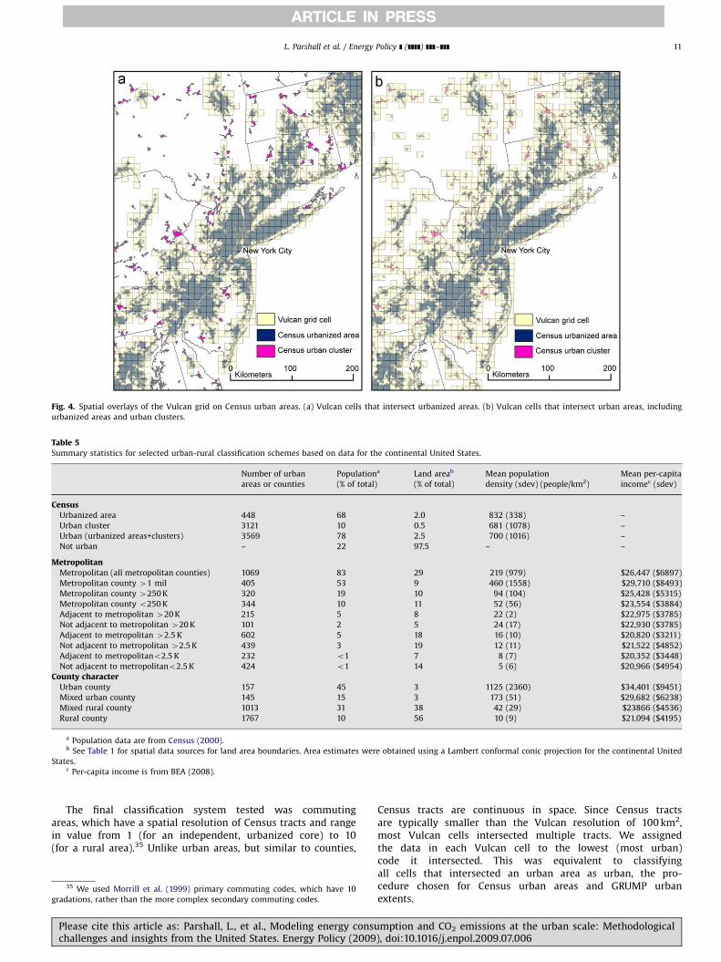
Census urban areas and GRUMP urban extents are notcontinuous in space. In other words, they define the extent ofeach urban area, but blank space in-between is simply ‘‘non-urban.’’ To estimate urban energy consumption, we classified allVulcan grid cells that intersected an urban area as ‘‘urban.’’ In thecase of the Census classification system, this included bothurbanized areas and urban clusters. Fig. 4 illustrates theimperfect match between the Vulcan grid and the Censusboundaries, which is particularly pronounced when small, urbanclusters are included. We considered weighting Vulcan data basedon the percent of the cell inside an urban boundary to avoidoverestimating urban energy consumption, but ultimately

decided against this since it is unlikely that the ‘‘urban’’and ‘‘rural’’ portion of these cells have the same energyconsumption per unit area. We also considered excluding cellsthat were below an overlap threshold—for example, cells thatwere less than 1%, 5%, or 10% urban. We conducted some simplet-tests to determine whether these border cells were significantlydifferent from rural and/or non-border urban cells. Since bordercells that were just 1% urban were significantly different fromrural cells, we chose to include all cells regardless of the extentof overlap.

We did not calculate energy consumption or CO2 emissions forindividual urban areas (as defined by the Census) because of thelimitations of the overlay methodology, which not only introducedpositive bias, but also raised questions about how to allocate data inVulcan cells that intersected more than one urban area. Thesechallenges reinforce the limitations of the Census urban boundariesas an appropriate spatial unit for local inventories as well as thedifficulty of working with the gridded version of the Vulcan dataproduct when dealing with political boundaries.

0

500

1000

1500

2000

2500

3000

500 1000 1500 2000 2500 3000

Correlation: 0.99RMSE: 63 TJ

Vulc

an (T

J)

0

500

1000

1500

2000

2500

3000

500 1000 1500 2000 2500 3000

Correlation: 0.87RMSE: 341 TJ(RMSE is 182 TJ with one outlier,not shown, removed)

Vulc

an (T

J)

0

400

800

1200

1600

2000

2400

400 800 1200 1600 2000 2400


Vulc

an (T

J)

0

200

400

600

800

1000

200 400 600 800 1000


Vulc

an (T

J)

0

400

800

1200

1600

2000

400 800 1200 1600 2000

Correlation: 0.89RMSE: 258 TJ(RMSE is 121 TJ with one outlier, not shown, removed)

Vulc

an (T

J)

0

100

200

300

400

100 200 300 400

Correlation: 0.45

Coal

Oil - diesel, distillate, residual

Buildings & industry

Natural Gas & LPG

Oil - gasoline

On-road transportation

Vulc

an (T

J)

EIA (TJ)

EIA (TJ)

EIA (TJ)

EIA (TJ)

EIA (TJ) EIA (TJ)

RMSE: 58 TJ

Fig. 3. Comparison between Vulcan fuel consumption and EIA fuel consumption in each state in 2002. (a) Coal. (b) Natural gas and LPG. (c) Oil–diesel, distillate, andresidual. (d) Oil–gasoline. (e) Buildings and industry (coal, natural gas, LPG, distillate fuel oil, residual fuel oil). (f) On-road transportation (gasoline, diesel).



ARTICLE IN PRESS

The final classification system tested was commutingareas, which have a spatial resolution of Census tracts and rangein value from 1 (for an independent, urbanized core) to 10(for a rural area).35 Unlike urban areas, but similar to counties,

Census tracts are continuous in space. Since Census tractsare typically smaller than the Vulcan resolution of 100 km2,most Vulcan cells intersected multiple tracts. We assignedthe data in each Vulcan cell to the lowest (most urban)code it intersected. This was equivalent to classifyingall cells that intersected an urban area as urban, the pro-cedure chosen for Census urban areas and GRUMP urbanextents.

Table 5Summary statistics for selected urban-rural classification schemes based on data for the continental United States.

Number of urbanareas or counties

Populationa

(% of total)Land areab

(% of total)Mean populationdensity (sdev) (people/km2)

Mean per-capitaincomec (sdev)

CensusUrbanized area 448 68 2.0 832 (338) –Urban cluster 3121 10 0.5 681 (1078) –Urban (urbanized areas+clusters) 3569 78 2.5 700 (1016) –Not urban – 22 97.5 – –

MetropolitanMetropolitan (all metropolitan counties) 1069 83 29 219 (979) $26,447 ($6897)Metropolitan county 41 mil 405 53 9 460 (1558) $29,710 ($8493)Metropolitan county 4250K 320 19 10 94 (104) $25,428 ($5315)Metropolitan county o250K 344 10 11 52 (56) $23,554 ($3884)Adjacent to metropolitan 420K 215 5 8 22 (2) $22,975 ($3785)Not adjacent to metropolitan 420K 101 2 5 24 (17) $22,930 ($3785)Adjacent to metropolitan 42.5K 602 5 18 16 (10) $20,820 ($3211)Not adjacent to metropolitan 42.5K 439 3 19 12 (11) $21,522 ($4852)Adjacent to metropolitano2.5K 232 o1 7 8 (7) $20,352 ($3448)Not adjacent to metropolitano2.5K 424 o1 14 5 (6) $20,966 ($4954)

County characterUrban county 157 45 3 1125 (2360) $34,401 ($9451)Mixed urban county 145 15 3 173 (51) $29,682 ($6238)Mixed rural county 1013 31 38 42 (29) $23866 ($4536)Rural county 1767 10 56 10 (9) $21,094 ($4195)

a Population data are from Census (2000).b See Table 1 for spatial data sources for land area boundaries. Area estimates were obtained using a Lambert conformal conic projection for the continental United

States.c Per-capita income is from BEA (2008).

Fig. 4. Spatial overlays of the Vulcan grid on Census urban areas. (a) Vulcan cells that intersect urbanized areas. (b) Vulcan cells that intersect urban areas, includingurbanized areas and urban clusters.

35 We used Morrill et al. (1999) primary commuting codes, which have 10gradations, rather than the more complex secondary commuting codes.



ARTICLE IN PRESS

3.3. Comparing localities on the basis of per-capita consumption

A straightforward way to compare localities is on the basis ofper-capita consumption. Population data for each set of spatialboundaries were obtained from the US Census (2000).36

0%

10%

20%

30%

40%

50%

60%

70%

80%

90%

100%

Census GRUMP Metro Continuum Character CommutingAdjacent = adjacent to a metropolitan area

0%

10%

20%

30%

40%

50%

60%

70%

80%

90%

100%

Census GRUMP Metro Continuum Character CommutingHigh = high commutingLow = low commutingLarge = large town coreSmall = small town core

High = high commutingLow = low commutingLarge = large town coreSmall = small town core

Adjacent = adjacent to a metropolitan area

Fig. 5. Percent of direct fuel consumption that occurs in urban areas based on a range of different urban/rural classification systems. (a) Buildings and industryconsumption of coal, natural gas, LPG, distillate fuel oil, and residual fuel oil. (b) Gasoline and diesel consumption on roadways. Refer to Table 1 for more information abouturban/rural classification systems.

36 Although Vulcan data are for 2002, we do not use 2002 estimates availablethrough the Census Bureau’s American Community Survey (ACS) for selected

(footnote continued)spatial boundaries, nor do we adjust the Census data to reflect population changesbetween 2000 and 2002. This was done to avoid introducing error by makingprojections at different spatial scales and/or through mixing ACS sample data withdata from the Decennial Census. Since population grew by just 0.3% between 2000and 2002, and since changes in the spatial distribution of population are likely tohave been equally small, this is not likely to be a large source of error in our per-capita estimates.



ARTICLE IN PRESS

To compare per-capita consumption with per-capita income, weused county-scale data on per-capita income from the Bureau ofEconomic Analysis (US BEA, 2008).37

Table 5 summarizes population and per-capita income data forselected urban/rural classification schemes. The populationdistribution is highly skewed: 68% of the population lives inurbanized areas that span just 2% of the land area, more than halfof whom live in large, urbanized areas with more than 1 millionpeople. Thus, urban/rural classification systems generally showgreater population variance in urban categories than in ruralcategories, which can increase the difficulty of deriving an urbanthreshold that groups localities with similar character.

One classification system that does not exhibit this propertyis Census urban areas: the standard deviation of populationdensity in less dense urban clusters is higher than in denserurbanized areas. Urban areas are constructed block by block,with stricter requirements for urbanized areas than urbanclusters, explaining the lower variance in population density.But classification systems based on jurisdictional boundaries areappealing from the perspective of benchmarking and targetsetting.

4. Results

We find that, depending on the definition of urban, between37% and 86% of direct fuel consumption in buildings and industryand between 37% and 77% of on-road gasoline and dieselconsumption occurs in urban areas (Fig. 5). Results were similarfor both sectors, although we found that the urban share of fuelconsumption tended to be higher for buildings and industrycompared with the transportation sector. We report all results inenergy units, rather than compare energy and CO2 emissions,because the exclusion of electricity means the two are highlycorrelated within each sector.38 A detailed analysis of differencesbetween local energy consumption and CO2 emissions is beyondthe scope of this paper.

Along with metropolitan areas, Census urban areas andGRUMP urban extents were at the upper end of this range.For example, 76% of direct final consumption occurs in Censusurban areas, with 59% occurring in urbanized areas and 17%occurring in urban clusters.39 However, it is likely that urbanenergy consumption was overestimated for the latter two spatialscales due to error introduced by the imperfect match between

Table 6Ratios between direct final consumption per capita in each urban/rural category and average direct final consumption per capita in the United States.

Classification system Buildings and industry On-road transportation Total direct fuel consumption

Natural gas and LPG Fuel oil Gasoline Diesel

CensusUrbanized area 0.95 0.88 0.83 0.70 0.87Urban cluster 1.71 2.15 1.32 1.57 1.63Urban (urbanized areas+clusters) 1.05 1.05 0.89 0.82 0.97Not urban 0.80 0.80 1.41 1.68 1.12

Metropolitan countiesMetropolitan (all metropolitan counties) 0.96 0.91 0.95 0.87 0.94Metropolitan county 41 mil 0.89 0.64 0.91 0.75 0.84Metropolitan county 4250K 1.09 1.23 1.02 1.01 1.08Metropolitan countyo250K 1.09 1.67 1.06 1.26 1.16Adjacent to metropolitan 420K 0.93 1.20 1.14 1.39 1.12Not adjacent to metropolitan 420K 1.31 0.86 1.05 1.27 1.18Adjacent to metropolitan 42.5K 1.45 2.04 1.35 1.84 1.51Not adjacent to metropolitan 42.5K 1.52 1.20 1.28 1.71 1.40Adjacent to metropolitano2.5K 0.69 3.02 1.57 2.17 1.88Not adjacent to metropolitano2.5K 1.19 0.72 1.46 1.95 1.32

County characterUrban county 0.92 0.67 0.88 0.66 0.84Mixed urban county 0.85 0.69 0.98 0.93 0.88Mixed rural county 1.15 1.50 1.08 1.24 1.17Rural county 1.19 1.46 1.40 1.92 1.42

CommutingUrban core 0.99 0.96 0.89 0.77 0.92High commuting to urban core 1.06 0.77 1.76 1.99 1.37Low commuting to urban core 1.06 1.09 2.03 2.47 1.54Large town core 1.19 1.58 0.82 1.01 1.12High commuting to large town core 1.14 1.13 1.56 1.99 1.35Low commuting to large town core 1.42 4.52 1.20 1.48 1.60Small town core 1.12 0.91 1.00 1.37 1.08High commuting to small town core 0.78 0.38 1.24 1.59 0.98Low commuting to small town core 0.34 0.41 0.91 1.08 0.61Rural 0.69 0.98 0.94 1.22 0.94

A value of 0.87 for total direct final consumption in urbanized areas indicates that the typical resident of an urbanized area consumes 13% less energy than the typical USresident.

37 The Census releases estimates of per-capita income based on pre-tax cashincome, but the BEA estimates are more complete. Ruser et al. (2004) describes thedifferences between the two datasets. BEA data are not available at higherresolution than counties. Although per-capita income data are available throughthe Census down to the block scale, aggregating these data to estimate per-capitaincome in each Census urban area was beyond the scope of our analysis.

38 At the county scale, the correlation between buildings and industry energyconsumption and CO2 emissions is 0.99 and the correlation between transporta-tion energy consumption and CO2 emissions is also 0.99.

39 Note that the 76% figure for direct final consumption in US urban areas islower than the 80% figure reported in the IEA analysis. Although Vulcan was usedin both analyses, the methodology was different. Also, unlike the present analysis,the IEA analysis included final consumption of electricity.



ARTICLE IN PRESS

Vulcan grid cells and urban boundaries in the spatial overlays.Therefore, we compared our estimate of metropolitan areaconsumption obtained from Vulcan county-scale data with anestimate obtained by overlaying the Vulcan 100km2 grid onmetropolitan area boundaries. The estimate obtained from thespatial overlay was 15% higher than the estimate obtained fromthe raw county-scale data, a substantial difference, but notsufficient to eliminate the gap between the upper and lower endof the range. This confirms that estimates of urban energyconsumption are sensitive to spatial scale. The relatively largeerror introduced by the overlays also demonstrates that trackingenergy and emissions data by administrative boundaries ispreferable.

Although urban areas are responsible for the majority of directfuel consumption, they tend to consume less fuel per capita(Table 6). The differences are most pronounced for morerestrictive definitions of urban such as counties with urbancharacter, Census urbanized areas, and metropolitan countieswith more than 1 million people. Based on these definitions, per-capita energy consumption in urban areas is 13–16% lowercompared with the national average. Smaller urban clusters andmetropolitan counties with fewer than 1 million people tend toconsume more energy per capita than the US average, so whenthese areas are included, urban residents appear to consume just3–6% less than the average US resident. This suggests that thechoice of urban threshold can have as large an impact on results asthe choice of spatial boundaries.

Fig. 6a and b show that per-capita energy consumption inurban counties varies less than per-capita energy consumption inrural counties, particularly in the transportation sector, suggestinga threshold effect above which urban areas converge on a lower

level of direct fuel consumption per capita. This effect also existsin comparisons between metropolitan and non-metropolitancounties, but to a lesser degree (Fig. 6c and d). Classifyingcounties based on urban/rural character may strengthen theurban signal by picking up urban attributes, such as reduced useof personal transportation, which are obscured by grouping urbanand suburban portions of metropolitan areas. The weaker signalfor buildings and industry compared with transportation is likelyrelated to the strong effect of climate on heating demand inbuildings as well as substantial variation in commercial andindustrial energy use. Fig. 7 confirms that, although urban

0

50

100

150

200

250 500 750 1000

Tota

l (PJ

)

Per capita (GJ/person)

0

50

100

150

200

250 500 750 1000

Tota

l (PJ

)


0

50

100

150

200

250 500 750 1000

Rural Mixed rural Mixed urban Urban

Tota

l (PJ

)


Non-metropolitan Metropolitan Non-metropolitan Metropolitan

0

50

100

150

200

250 500 750 1000

Tota

l (PJ

)


Rural Mixed rural Mixed urban Urban

Fig. 6. County per-capita consumption versus county total consumption. (a) Direct energy consumption in buildings and industry, with counties classified by urban/ruralcharacter. (b) Direct energy consumption for transportation, with counties classified by urban/rural character. (c) Direct energy consumption in buildings and industry, withcounties classified as metropolitan or non-metropolitan. (d) Direct energy consumption for transportation, with counties classified as metropolitan or non-metropolitan.Note that a small number of outliers are not shown on the scatter plots. PJ ¼ Petajoule ¼ 1015 J. GJ ¼ Gigajoule ¼ 109 J.

0

500

1000

1500

2000

10,000 20,000 30,000 40,000 50,000

RuralMixed ruralMixed urbanUrban

Per c

apita

(GJ/

pers

on)

Per-capita income (USD)

Fig. 7. County per-capita income versus county per-capita consumption, withcounties classified by urban/rural character. Note that a small number of outliersare not shown on the scatter plot.



ARTICLE IN PRESS

counties have higher mean per-capita income, there is norelationship between per-capita energy consumption and per-capita income in urban localities.

These findings are not intended to contribute to debates on theunderlying mechanisms through which urbanization affectspatterns of energy consumption and CO2 emissions. Rather, ourintention is to suggest that a national inventory at the local scaleshould allow for meaningful comparisons of localities with similarcharacter, and that this requires choosing a spatial scale and urbandefinition for which the ‘‘urban’’ signal clearly differs from the‘‘rural’’ signal.

5. Toward a national inventory at the local scale

Through our analysis of urban energy consumption in theUnited States, we have shown that the following factors areimportant to the design of a national inventory of local-scaleenergy use and related CO2 emissions: consistency, spatialresolution, accounting framework, and attributes.

5.1. Consistency

The inventory should be built from systematic data collectedfor the entire country. Ideally, all raw data underlying theinventory should be derived from comparable energy-sectordata on location-specific fuel consumption. In practice, compar-able sources of raw data for all sectors and fuels may beimpossible to find, and some data may be derived from emissionsmodels rather than from raw energy data. The consistency of theraw data within each sector is probably more important than theconsistency across sectors. Data sources, and protocols forsynthesizing data into an inventory, should facilitate the releaseof inventories at regular intervals. Responsibility for dataorganization and synthesis should be centralized at a singleinstitution, preferably a government agency, to ensure that dataproducts are recognized as authoritative and are available to thepublic.

5.2. Spatial resolution

The spatial resolution should match the smallest set ofcontinuous administrative boundaries at which energy data areavailable for the entire United States. Examples of continuousboundaries in the country are: states, counties, Census tracts,Census block groups, and Census blocks. Currently, counties arethe highest resolution at which energy data are available.Choosing continuous boundaries, rather than discontinuousboundaries such as Census urban areas or metropolitan areas,allows for complete coverage of the country at a high spatialresolution and allows analysis at multiple spatial scales. Forexample, county-scale data can be aggregated to analyzemetropolitan areas, micropolitan areas, and/or combined statis-tical areas in the United States.

5.3. Accounting framework

The inventory should be constructed according to a clearlydefined accounting framework. The accounting framework shoulddefine the energy system perspective, including whether theinventory will cover direct final consumption, total final con-sumption, or total primary energy supply; how the inventory willallocate point source and non-point source data to localities;which fuels and/or sectors will be covered, and the scope of eachsector; and how the inventory will partition data. For example, the

inventory might categorize data by fuel, sector, sector and fuel, orsector and end use.40

5.4. Attributes

In addition to energy and CO2 emissions data, the inventoryshould include consistent data for each locality on total popula-tion and spatial area. It also should designate the locality as urbanor rural. These are the minimum attributes required to makemeaningful cross-locality comparisons. Linking the inventory toadditional climate, socio-demographic, and economic indicatorswould help facilitate analysis of interactions between thesefactors and energy consumption and emissions.

In Fig. 8, we present maps illustrating various inventory resultsbased on our analysis with the Vulcan data product, the mostconsistent dataset available in the United States. The spatialresolution is counties, which are continuous in space. Theaccounting framework is direct final consumption, and we showresults for the sector-fuel combination of gasoline consumption inthe transportation sector. We compare totals for each county(Fig. 8a) as well as per-capita totals (Fig. 8b). We normalizedresults by dividing by the mean. In Fig. 8a and b, a value of 100%indicates that the county’s consumption is no different from theaverage across all counties in the continental United States. InFig. 8c, we show per-capita results normalized by the mean forcounties with the same character. In this case, a value of 100%for an urban county indicates that the county’s per-capitaconsumption is no different from the average across all urbancounties in the continental United States. Closely comparingFig. 8b and c reveals subtle differences. For example, Fig. 8b showsthat the counties representing the urban core of Los Angelesconsume 50–75% less gasoline per-capita than the nationalaverage, but 75–100% as much gasoline as the average urbancounty. Similar differences can be seen for Miami.

6. Conclusions, policy applications, and recommendations

The number of local authorities interested in addressingenergy and climate concerns has been growing at the same timethat new funding sources for local energy efficiency measures arebecoming available. For example, the 2007 Energy Independenceand Security Act established the Energy Efficiency and Conserva-tion Block Grant Program, a $2 billion per year pool of funds thatcities and counties around the country can use for energyefficiency and conservation plans and programs.41 In early 2009,the US stimulus bill authorized funding for this program.42 Sincefunds can be spent on planning as well as program implementa-tion, baseline studies of energy consumption and CO2 emissionsare likely to proliferate. An established inventory process couldensure that baseline studies are standardized and comparable,helping localities set reasonable targets for different fuels andsectors. High-resolution data made available through inventoriescan also support research on the relationships between energyconsumption, urban form, economic development, and socio-demographic patterns in the United States. Conducting inven-tories at regular intervals could help localities monitor changesover time and evaluate how local policies may be affecting energyand emissions trajectories.

40 Bennett and Newborough (2001) discuss energy audits for cities brokendown by sector and end use.

41 The Energy Efficiency Block Grant program is described in US Conference ofMayors (2008).

42 A statement from the US Conference of Mayors is available in PR Newswire(2009).



ARTICLE IN PRESS

Fig. 8. Patterns of gasoline consumption across US counties. (a) County gasoline consumption compared to US average consumption. A value of 100% indicates that thecounty has the same total gasoline consumption as the average county in the US. (b) County per-capita gasoline consumption compared to country-wide per-capitaconsumption. (c) County per-capita gasoline consumption compared to per-capita average for corresponding character class.



ARTICLE IN PRESS

Carbon markets are another potential source of funds.For example, the Regional Greenhouse Gas Initiative in thenortheastern United States is likely to generate some funding forcity-based energy efficiency initiatives. The city of San Francisco istrying to establish its own voluntary carbon market, throughwhich it would sell emission reduction credits to organizationsand individuals seeking to offset their own carbon emissions anduse the proceeds to support local energy efficiency projects. Well-functioning carbon markets require strict monitoring protocols,reinforcing the need for consistent data and a coherent accountingframework.

While some mayors are emerging as leaders in the local energypolicy arena, there is no federal mandate under which individualcities and towns are required to report their energy consumptionor CO2 emissions. We have proposed counties as the best spatialscale for a local inventory because raw energy data are available atthis scale, counties are a recognized political unit with someauthority to formulate local policy, and some cities are defined bycounty boundaries (e.g. Denver, Colorado) or groups of counties(e.g., New York City is 5 counties). A county-scale inventory wouldmost directly support county-scale initiatives. But since countiesrarely have the same energy policy powers available to localauthorities (e.g., waste, land use, transport planning) or stategovernment (e.g., building codes), elevating the locus of energyplanning efforts to counties is problematic. An alternative is torefine federally mandated reporting requirements so that smallerentities (e.g. individual cities and towns) are required to regularlyreport emissions, a step that would likely require congressionalaction.

In this paper, we excluded the electricity sector from ouranalysis. Inventorying electricity consumption would help local-ities understand where their power comes from and clarify localdifferences in the carbon intensity of energy consumption.Changing the mandatory reporting requirements might enablethis, but would likely require the involvement of the FederalEnergy Regulatory Commission (FERC), state-level electricityregulatory agencies, and Independent System Operators (ISO).The potential costs of pursuing a change in reporting should bebalanced against the capacity of local authorities to influencepower supply mix. For example, a national cap-and-trade programor carbon tax targeting the power sector might leave little spacefor local authorities to influence the local fuel mix.

Moving toward a national inventory at the local scale requiresbetter coordination between Vulcan-type efforts to synthesizeavailable data and local stakeholders. Currently, Vulcan is themost comprehensive and systematic effort to develop a high-resolution CO2 emissions inventory for the United States. Werecommend that Vulcan be used as the starting point for the nextphase of inventory development. Coordination with similar effortsin other countries and/or with efforts to inventory other GHGs athigh resolution could facilitate the development of internationallyrecognized standards for local-scale energy and emissionsinventories, which could help to identify low-energy and low-carbon pathways in a range of different local settings.

Acknowledgements

We gratefully acknowledge the support of the Center forEnergy, Marine Transportation and Public Policy (CEMTPP) at theSchool of International Affairs and Public Affairs (SIPA), ColumbiaUniversity. We thank the International Energy Agency andparticularly Nigel Jollands and Paul Dowling; the Project Vulcanresearch team based at Purdue University including Broc Seib andWilliam Ansley of the Rosen Center for Advanced Computing;Marc Fischer and Stephane de la Rue du Can of Lawrence Berkeley

National Laboratory; Dennis Ojima, Scott Denning, Kathy Corbin,and Steve Knox of Colorado State University; and AndrewIsserman at the University of Illinois at Urbana-Champaign.

References

Bennett, M., Newborough, M., 2001. Auditing energy use in cities. Energy Policy 29,125–134.

Bento, A.M., Cropper, M.L., Mobarak, A.M., Vinha, K., 2005. The effects of urbanspatial structure on travel demand in the United States. The Review ofEconomics and Statistics 87 (3), 466–478.

Brown, M., Southworth, F., Sarzynski, A., 2008. Shrinking the carbon footprint ofmetropolitan America. Brookings Institute Metropolitan Policy Program.Available at: /http://www.brookings.edu/reports/2008/05_carbon_footprint_sarzynski.aspxS, accessed February 2009.

Brown, M., Logan, E., 2008. The residential energy and carbon footprints of the 100largest US metropolitan areas. Georgia Institute of Technology School of PublicPolicy Working Papers, 39. Available at: /http://smartech.gatech.edu/dspace/handle/1853/22228S, accessed February 2009.

CARMA, 2008. Carbon Monitoring for Action. Available at: /www.carma.orgS,accessed September 2008.

Center for International Earth Science Information Network (CIESIN), ColumbiaUniversity; International Food Policy Research Institute (IFPRI), the WorldBank; and Centro Internacional de Agricultura Tropical (CIAT), 2004. GlobalRural–Urban Mapping Project (GRUMP): Urban Extents. Palisades, NY: CIESIN,Columbia University. Data available at: /http://sedac.ciesin.columbia.edu/gpw/global.jspS, accessed September 2008.

City of Paris, 2008. Le bilan carbone. Available at: /http://www.paris.fr/portail/Environnement/Portal.lut?page_id=8414&document_type_id=5&document_id=14612&portlet_id=19612S, accessed February 2009.

Ewing, R., Rong, F., 2008. The impact of urban form on US residential energy use.Housing Policy Debate 19 (1), 1–30.

Glaeser, E.L., Kahn, M.E., 2008. The Greenness of Cities. Rappaport Institute forGreater Boston and Taubman Center for State and Local Government PolicyBriefs. Available at: /www.hks.harvard.edu/rappaport/downloads/policybriefs/greencities_final.pdfS, accessed February 2009.

Gurney, K.R., Seib, B., Ansley, W., Mendoz, D., Miller, C., Fischer, M., 2008. VulcanScience Methods Documentation. Project Vulcan, Purdue University. Alsosee: /http://www.purdue.edu/eas/carbon/vulcan/research.htmlS, accessedOctober 2008.

Gurney, K.R., Mendoza, D., Zhou, Y., Fischer, M., de la Rue du Can, S., Geethakumar,S., Miller, C., 2009. The Vulcan project: high resolution fossil fuel combustionCO2 emissions fluxes for the United States. Environmental Science andTechnology 43 (14), 5535–5541.

Holden, E., Norland, I.T., 2005. Three challenges for the compact city as asustainable urban form: household consumption of energy and transport ineight residential areas in the greater Oslo region. Urban Studies 42 (12),2145–2166.

International Council for Local Environmental Initiatives (ICLEI), 2008a.Regional Membership Lists. /http://www.iclei.org/index.php?id=800S,accessed January 2009.

International Council for Local Environmental Initiatives (ICLEI), 2008b. Interna-tional Local Government GHG Emissions Analysis Protocol Release Version 1.0.Available at: /http://www.iclei.org/index.php?id=8154S, accessed February2009.

International Energy Agency (IEA), 2008. World Energy Outlook 2008. OECD/IEA.578 pages. Also see: /www.worldenergyoutlook.org/docs/weo2008/WEO_2008_Energy_Use_in_Cities_Modelling.pdfS, accessed January 2009.

Isserman, A.M., 2005. In the national interest: defining rural and urban correctly inresearch and public policy. International Regional Science Review 28, 465–499.

Kahn, M.E., 2000. The environmental impact of suburbanization. Journal of PolicyAnalysis and Management 19 (4), 569–586.

Lakhina, A., Byers, J.W., Crovella, M., Matta, I., 2003. On the geographic location ofinternet resources. IEEE Journal on Selected Areas in Communications 21 (6),934–948.

Lenzen, M., Pade, L., Munksgaard, J., 2004. CO2 multipliers in multi-region input-output models. Economic Systems Research 16 (4), 391–412.

Morrill, R., Cromartie, J., Hart, G., 1999. Metropolitan, urban, and rural commutingareas: toward a better depiction of the United States settlement system. UrbanGeography 20 (8), 727–748.

Moyers, P., O’Leary, R., Helstroom, R., 2005. Multi-unit residential building energyand peak demand study. Energy News 23 (4), 113–116.

Naess, P., Sandberg, S.L., Roe, P.G., 1996. Energy use for transportation in 22 Nordictowns. Scandinavian Housing and Planning Research 13, 79–97.

National Atlas of the United States and the United States Geological Survey(National Atlas), 2006. US National Atlas Urbanized Areas Redlands, California,USA: ESRI. Data available at: /https://www1.columbia.edu/sec/acis/eds/dgate/studies/C1301/data/ESRI_2006_usa_urban_dtl.zipS, accessed September 2008.

New York City Office of Long Term Planning and Sustainability (NYC OLTPS), 2008.Personal communication with Jonathan Dickinson, Senior Policy Advisor,New York City Office of Operations, Office of Long Term Planning andSustainability.

Petron, G., Tans, P., Frost, G., Chao, D., Trainer, M., 2008. High-resolution emissionsof CO2 from power generation in the USA. Journal of Geophysical Research 113.



http://www.brookings.edu/reports/2008/05_carbon_footprint_sarzynski.aspx

http://www.brookings.edu/reports/2008/05_carbon_footprint_sarzynski.aspx

http://smartech.gatech.edu/dspace/handle/1853/22228


http://sedac.ciesin.columbia.edu/gpw/global.jsp

http://sedac.ciesin.columbia.edu/gpw/global.jsp

http://www.paris.fr/portail/Environnement/Portal.lut?page_id=8414&document_type_id=5&document_id=14612&portlet_id=19612






http://www.purdue.edu/eas/carbon/vulcan/research.html

http://www.iclei.org/index.php?id=800

http://www.iclei.org/index.php?id=8154

https://www1.columbia.edu/sec/acis/eds/dgate/studies/C1301/data/ESRI_2006_usa_urban_dtl.zip

https://www1.columbia.edu/sec/acis/eds/dgate/studies/C1301/data/ESRI_2006_usa_urban_dtl.zip

ARTICLE IN PRESS

PR Newswire, 2009. US Mayors Commend Final Economic Recovery Bill. Availableat: /http://news.prnewswire.com/DisplayReleaseContent.aspx?ACCT=ind_focus.story&STORY=/www/story/02-13-2009/0004972282&EDATES, accessed March2009.

Randolph, J., 2008. Comment on Reid Ewing and Fang Rong’s ‘‘The impact of urbanform on US residential energy use’’. Housing Policy Debate 19 (1), 45–52.

Ruser, J., Pilot, A., Nelson, C., 2004. Alternative measures of household income: BEApersonal income, CPS money income, and beyond. Available at: /www.bea.gov/about/pdf/AlternativemeasuresHHincomeFESAC121404.pdfS, accessedFebruary 2009.

Satterthwaite, D., 2008. Cities’ contribution to global warming: notes on theallocation of greenhouse gas emissions. Environment and Urbanization 20 (2),539–549.

Schipper, L., 1995. Determinants of automobile use and energy consumptionin OECD countries. Annual Review of Energy and the Environment 20,286–325.

Southworth, F., Sonenberg, A., Brown, M., 2008. The transportation energy andcarbon footprints of the 100 largest US metropolitan areas. Georgia Institute ofTechnology School of Public Policy Working Papers, 37. Available at: /http://smartech.gatech.edu/dspace/handle/1853/22231S, accessed February 2009.

Staley, S.R., 2008. Missing the forest through the trees? Comment on Reid Ewingand Fang Rong’s ‘‘The impact of urban form on US residential energy use’’.Housing Policy Debate 19 (1), 31–43.

Tele Atlas North America, Inc./Geographic Data Technology, Inc. (Tele Atlas), 2005.US Core Based Statistical Areas Redlands, California, USA: ESRI. Data availableat: /http://www1.columbia.edu/sec/acis/eds/dgate/studies/C1301/data/ESRI_2005_united_states_cbsa.zipS, accessed September 2008.

Tele Atlas North America, Inc., 2006. US Populated Place Areas Redlands, California,USA: ESRI. Data available at: /http://www1.columbia.edu/sec/acis/eds/dgate/studies/C1301/data/ESRI_2006_usa_placeply.zipS, accessed September 2008.

United States Conference of Mayors, 2008. The Energy Efficiency and ConservationBlock Grant (EECBG) Handout. Available at: /http://usmayors.org/climateprotection/documents/eecbghandout.pdfS, accessed March 2009.

United Nations Statistics Division (UN), 2009. Population density and urbanization.Available at: /http://unstats.un.org/unsd/demographic/sconcerns/densurb/densurbmethods.htmS, accessed January 2009.

United States Department of Agriculture (USDA), 2003a. Measuring Rurality:Rural–Urban Continuum Codes, 2003 version. USDA Economic ResearchService. Coding scheme originated by D.L. Brown, F.K. Hines, and J.M. Zimmerin Social and Economic Characteristics of the Population in Metro andNonmetro Counties: 1970. Data available at: /http://www.ers.usda.gov/briefing/rurality/ruralurbcon/S, accessed September 2008.

United States Department of Agriculture (USDA), 2003b. Measuring Rurality:Urban Influence Codes, 2003 version. USDA Economic Research Service. Dataavailable at: /http://www.ers.usda.gov/Briefing/Rurality/UrbanInf/S, accessedSeptember 2008.

United States Department of Commerce, Bureau of Economic Analysis (US BEA),2008. Regional Economic Accounts. Available at: /http://www.bea.gov/regionalS accessed November 2008.

United States Department of Commerce, Census Bureau, Geography Division (USCensus), 2000. US Census Urbanized Areas Redlands, California, USA: ESRI.Data available at: US BEA, accessed September 2008.

United States Department of Energy (US DOE), 2005. Residential EnergyConsumption Survey, Energy Information Administration. Available at:/http://www.eia.doe.gov/emeu/recs/S, accessed March 2009.

United States Department of Energy (US DOE), 2008a. Annual Energy Review 2007,Energy Information Administration. Available at: /http://www.eia.doe.gov/aer/S, accessed November 2008.

United States Department of Energy (US DOE), 2008b. Electricity Database Files,Energy Information Administration. Available at: /http://www.eia.doe.gov/cneaf/electricity/page/data.htmlS, accessed March 2009.

United States Department of Energy (US DOE), 2008c. State Energy Data System(SEDS), Energy Information Administration. Available at:/http://www.eia.doe.gov/emeu/states/_seds.htmlS, accessed September 2008.

United States Department of Transportation (US DOT), 2009. National HouseholdTravel Survey. Available at: /http://nhts.ornl.gov/S, accessed February2009.

United States Environmental Protection Agency (US EPA), 2008 eGRID. Available at:/http://www.epa.gov/cleanenergy/energy-resources/egrid/index.htmlS, ac-cessed September 2008.

Weber, C.L., Matthews, H.S., 2007. Quantifying the global and distributional aspectsof American household carbon footprint. Ecological Economics 66, 379–391.



http://news.prnewswire.com/DisplayReleaseContent.aspx?ACCT=ind_focus.story&STORY=/www/story/02-13-2009/0004972282&EDATE






http://www1.columbia.edu/sec/acis/eds/dgate/studies/C1301/data/ESRI_2005_united_states_cbsa.zip

http://www1.columbia.edu/sec/acis/eds/dgate/studies/C1301/data/ESRI_2005_united_states_cbsa.zip

http://www1.columbia.edu/sec/acis/eds/dgate/studies/C1301/data/ESRI_2006_usa_placeply.zip

http://www1.columbia.edu/sec/acis/eds/dgate/studies/C1301/data/ESRI_2006_usa_placeply.zip

http://usmayors.org/climateprotection/documents/eecbghandout.pdf

http://usmayors.org/climateprotection/documents/eecbghandout.pdf

http://unstats.un.org/unsd/demographic/sconcerns/densurb/densurbmethods.htm#B

http://unstats.un.org/unsd/demographic/sconcerns/densurb/densurbmethods.htm#B

http://www.ers.usda.gov/briefing/rurality/ruralurbcon/

http://www.ers.usda.gov/briefing/rurality/ruralurbcon/

http://www.ers.usda.gov/Briefing/Rurality/UrbanInf/

http://www.eia.doe.gov/emeu/recs/



http://www.eia.doe.gov/aer/

http://www.eia.doe.gov/aer/

http://www.eia.doe.gov/cneaf/electricity/page/data.html

http://www.eia.doe.gov/cneaf/electricity/page/data.html

http://www.eia.doe.gov/emeu/states/_seds.html

http://www.eia.doe.gov/emeu/states/_seds.html

http://nhts.ornl.gov/

Modeling energy consumption and CO2 emissions at the urban ...

Documents

Transcript of Modeling energy consumption and CO2 emissions at the urban ...