Modeling Crystallization in CMSMPR: Results of Validation Study on Population Balance Modeling in FLUENT

Bin Wan and Terry A. Ring Dept. Chemical Engineering

University of Utah Salt Lake City, UT 84112

and

Kumar M. Dhanasekharan and Jayanta Sanyal Fluent Inc.

10 Cavendish Court Lebanon, NH 03766

Abstract Fluent’s computational fluid dynamics environment has been enhanced with a population balance capability that operates in conjunction with its multiphase calculations to predict the particle size distribution within the flow field. The population balance is solved by one of the following methods; discrete method, standard method of moments, quadrature method of moments (QMOM). Fluent’s prediction capabilities are tested by using a 2-dimensional analogy of a constant stirred tank reactor with a fluid flow compartment that mixes the fluid quickly and efficiently using wall movements and has a feed stream and a product stream. The results of these Fluent simulations using QMOM population balance solver are compared to steady state analytical solutions for the population balance in a stirred tank where 1) nucleation, 2) growth, 3) aggregation, 4) breakage, take place separately and 5) combined nucleation and growth and combined nucleation, growth and aggregation takes place. The results of these comparisons show that the moments of the population balance are accurately predicted for nucleation, growth, aggregation and breakage when the flow field is turbulent. With laminar flow the mixing is not ideal and as a result the steady state well mixed solutions are not accurately simulated.

1. Introduction The population balance equation (PBE) is a statement of continuity for particulate systems. Cases in which a population balance could apply include crystallization, precipitation, bubble columns, gas sparging, sprays, fluidized bed polymerization, granulation, liquid-liquid dispersions, air classifiers, hydrocyclones, particle classifiers, and aerosol flows. In the case of a continuous mixed-suspension, mixed-product removal (CMSMPR) crystallizer in which aggregation, breakage and growth are occurring the PBE is given by Randolph and Larson (1) as

)()())()(()()( vdvbdv

vnvGdvnvn in −=+−τ

[1]

with the boundary condition, n(0)=no. In the above equation n(v) is the number-based population of particles in the tank which is a function of the particle volume, v. The subscript “in” refers to the inlet population. G(v) is the volume dependent growth rate and b(v) is the volume dependent birth rate and d(v) is the volume dependent death rate. In the case of aggregation the birth and death rate terms are given by Hulburt and Katz (2) as

∫∫∞

−−−=−0

2/

0)(),()()()(),()()( dwwnwvvndwwnwvnwwvvdvb

v

aa ββ [2]

where the aggregation rate constant, β(v,w), is a measure of the frequency of collision of particles of size v with those of size w. In the case of breakage, the birth and death rate terms are given by Prasher (3) as

)()()(),()()()( vnvSdwwnwvwSvdvbvbb −=− ∫∞

ρ [3]

where S(v) is the breakage rate constant that is a function of particle size, v, ρ(v,w) is the daughter distribution function defined as the probability that a fragment of a particle of size w will appear at size v. It is often useful to know the moments of n(v) because of physical significance. The kth volume moment is defined by

∫∞

=0

)( dwwnwm kkv [4]

vmo and vm1 represent the total number and total volume of particles in the system. The PBE can be transformed into a series of moment equations by multiplying equation 1 by vk and integrating with respect to v from zero to infinity. These moment equations are used in place of the PBE to approximate the particle size distribution, see Randolph and Larson (1). QMOM was first proposed by McGraw (4) and further developed by Marchisio, et. al. (5). With the QMOM PBE solver in Fluent, a small number of moments, N, (typically 6) are used. Moments are approximated by a quadrature approximation that uses N/2 weights, Wi, and N/2 sizes, Li, as follows:

∑=

=N

i

kiikL LWm

1 [5]

Upon substitution of these weights and sizes into the N moment equations, we have a series of equations that just equals the number of unknowns, N, allowing for the solution of the system of equations that constitutes an approximation of the PBE. From the moments the particle size distribution can be reconstituted using a moment transformation (1). For more details of this numerical method see the Fluent User’s Guide - Crystallization Sample Case and Data Files.

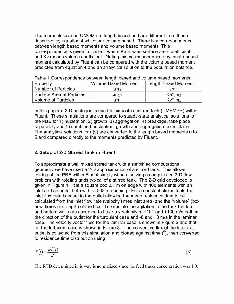
The moments used in QMOM are length based and are different from those described by equation 4 which are volume based. There is a correspondence between length based moments and volume based moments. This correspondence is given in Table I, where Ka means surface area coefficient, and Kv means volume coefficient. Noting this correspondence any length based moment calculated by Fluent can be compared with the volume based moment predicted from equation 4 and an analytical solution to the population balance. Table 1 Correspondence between length based and volume based moments Property Volume Based Moment Length Based Moment Number of Particles vm0 Lm0 Surface Area of Particles vm2/3 Ka*Lm2 Volume of Particles vm1 Kv*Lm3 In this paper a 2-D analogue is used to simulate a stirred tank (CMSMPR) within Fluent. These simulations are compared to steady-state analytical solutions to the PBE for 1) nucleation, 2) growth, 3) aggregation, 4) breakage, take place separately and 5) combined nucleation, growth and aggregation takes place. The analytical solutions for n(v) are converted to the length based moments 0 to 5 and compared directly to the moments predicted by Fluent.

2. Setup of 2-D Stirred Tank in Fluent To approximate a well mixed stirred tank with a simplified computational geometry we have used a 2-D approximation of a stirred tank. This allows testing of the PBE within Fluent simply without solving a complicated 3-D flow problem with rotating grids typical of a stirred tank. The 2-D grid developed is given in Figure 1. It is a square box 0.1 m on edge with 400 elements with an inlet and an outlet both with a 0.02 m opening. For a constant stirred tank, the inlet flow rate is equal to the outlet allowing the mean residence time to be calculated from the inlet flow rate (velocity times inlet area) and the “volume” (box area times unit depth) of the box. To simulate the agitation in the tank the top and bottom walls are assumed to have a y-velocity of +101 and +100 m/s both in the direction of the outlet for the turbulent case and -8 and +8 m/s in the laminar case. The velocity vector field for the laminar case is shown in Figure 2 and that for the turbulent case is shown in Figure 3. The convective flux of the tracer at outlet is collected from this simulation and plotted against time (6), then converted to residence time distribution using:

( )dttdCtE )(= [6]

The RTD determined in is way is normalized since the feed tracer concentration was 1.0.

Figure 1 Grid for 2-D simulation of well mixed stirred tank.

Figure 2 Velocity distribution for laminar flow Fluent simulation.

Figure 3 Velocity distribution for turbulent flow Fluent simulation. To test the accuracy of the well mixed assumption, the residence time distribution was predicted using a unit tracer concentration, a second phase with the properties of water, in the tank that is allowed to displace a first water phase as time progresses. The outlet concentration predicted by the simulation is shown in Figure 4 for the laminar flow and the turbulent flow simulations as well as the ideal curve. Here we see that the laminar flow curve has an initial peak above the ideal curve and a tail that is below the ideal curve. The turbulent simulation is nearly identical to the ideal curve.

0 50 100 1501 .10 3

0.01

0.1

Time (s)

E(t)

on lo

g ax

is

Figure 4 Comparison of Residence Time Distributions for Laminar (black line) and Turbulent (red dots) flow simulations with Ideal well mixed tank (green line). The mean and standard deviation of the various residence time distributions were determined giving the following comparison.

tmean/(V/Q) Error % Std.Deviation/tmean

Error %

Turbulence model 1.001 0.1 1.008 0.8

Laminar model 0.999 0.1 1.058 5.8

Ideal values for both the mean time, tmean, divided by the ratio of tank volume, V, to volumetric flow rate, Q and the standard deviation divided by the mean time should be 1.0. The laminar flow model is clearly worse than the turbulent flow model in approximating an idealized well mixed tank.

3. Numerical Case Studies Numerical cases, discussed below, have been developed to test the PBE capabilities of Fluent. First of all Fluent is used to solve the velocity field to a convergence of 10-5 for either the laminar or turbulent flow. Then the a multiphase calculation is initiated with the PBE solved by QMOM using 6 length based moments 0 to 5 (or more precisely 3 lengths and 3 weights) with the velocity field fixed. The convergence criterion is lowered to 10-7 (or lower) for the multiphase PBE calculation with a relaxation parameter of 0.9 except when otherwise stated. Case 1-Growth: The analytical solution to the PBE, equation [1], for growth alone was obtained by setting the growth rate to a constant (G(v)=G0), the

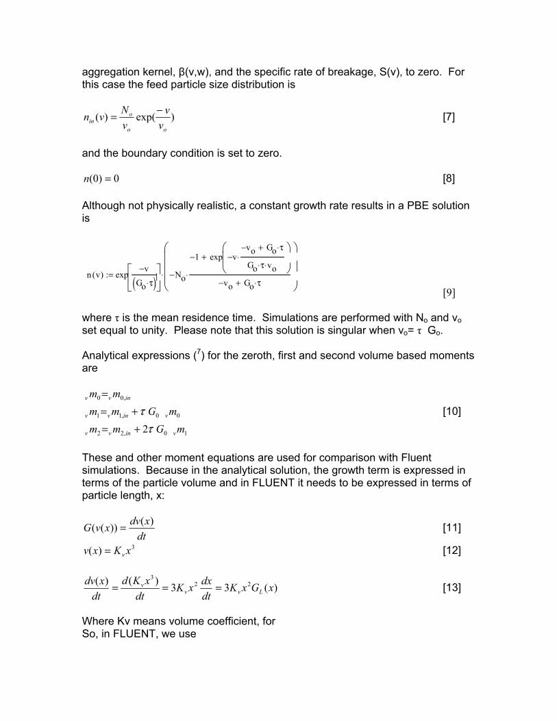
aggregation kernel, β(v,w), and the specific rate of breakage, S(v), to zero. For this case the feed particle size distribution is

)exp()(oo

oin v

vvNvn −= [7]

and the boundary condition is set to zero.

0)0( =n [8] Although not physically realistic, a constant growth rate results in a PBE solution is

n v( ) expv−

Go τ⋅( )

No−

1− exp v−vo− Go τ⋅+

Go τ vo⋅⋅⋅

+

vo− Go τ⋅+⋅

⋅:=

[9] where τ is the mean residence time. Simulations are performed with No and vo set equal to unity. Please note that this solution is singular when vo= τ Go. Analytical expressions (7) for the zeroth, first and second volume based moments are

10,22

00,11

,00

2 mGmmmGmm

mm

vinvv

vinvv

invv

ττ

+=+=

= [10]

These and other moment equations are used for comparison with Fluent simulations. Because in the analytical solution, the growth term is expressed in terms of the particle volume and in FLUENT it needs to be expressed in terms of particle length, x:

dtxdvxvG )())(( = [11]

3)( xKxv v= [12]

)(33)()( 223

xGxKdtdxxK

dtxKd

dtxdv

Lvvv === [13]

Where Kv means volume coefficient, for So, in FLUENT, we use

23))(()(xKxvGxG

vL = [14]

For the Fluent simulation the growth rate of 1 µm/s and the mean residence time of 100s was used with the initial particle size distribution in the tank given by the feed distribution, the simulation took 1600 iterations to achieve a convergence criterion of 10-9 for the turbulent flow simulation with a relaxation factor of 1.0 and 4000 iterations to achieve a convergence criterion of 10-9 for the laminar flow simulation. The results of these simulations are given in Table 2 for both the laminar and turbulent flow simulations with a relaxation factor of 0.9. The turbulent flow case will not converge with a relaxation factor of 1.0. The results of the turbulent flow simulation are accurate to only 0.2% with this convergence criterion. The results of the laminar flow simulation is less accurate – a 3.7% error with the same convergence criterion. Because the laminar flow simulation does not correspond to well-mixed conditions, it does not accurately simulate the analytical solution. Table 2 Moment comparison of PBE for Fluent Simulations with Analytical Solution for Growth

Turbulence Laminar Inlet Outlet

(Analytical) Outlet (Fluent)

Error %

Outlet (Fluent)

Error %

Lm0 1 1 1 0 1 0 Lm1 1.108 5.183 5.1906333 0.147 5.0913844 1.768 Lm2 1.39 30.227 30.251846 0.082 29.813738 1.367 Lm3 1.91 192.896 193.02859 0.069 192.86899 0.014 Lm4 2.821 1.323e3 1325.7223 0.206 1347.62 1.861 Lm5 4.423 9.626e3 9641.8662 0.165 9985.3242 3.733

Case 2-Nucleation and Growth: The analytical solution to the PBE, equation [1], for nucleation and growth was obtained by setting the growth rate to a constant (G(v)=G0), the aggregation kernel, β(v,w), and the specific rate of breakage, S(v), to zero. For this case the feed particle size distribution is set to zero, nin(v)=0 and the boundary condition is

onn =)0( [15] where no is the number density of particles with a zero size. The nucleation rate is given by the product of Go and no. The analytical solution for this case is given by (1)

)exp()(τo

o Gvnvn −= [16]

This analytical solution is converted to length based moments for comparison with the Fluent simulation. The Fluent simulation was run with GL-0=0.01 mm/s noting the above conversion in equations 11 to14 and the nucleation rate is 1#/m3/s, the mean residence time, τ, of 100s with no particles in the feed. The results of this comparison are given in Table 3. Here we see that the laminar flow simulation is in error by as much as ~25% while the turbulent flow simulation is accurate to ~0.01%. Table 3 Moment comparison of PBE for Fluent Simulations with Analytical Solution for Nucleation and Growth.

FLUENT FLUENT Analytical Solution Laminar Error% Turbulence Error%

Lm0 100 99.98 0.02 99.987236 0.013 Lm1 100 105.68 5.68 99.98867 0.011 Lm2 200 223.2 11.6 199.97765 0.011 Lm3 600 702.3 17.5 599.93298 0.012 Lm4 2400 2917.2 21.55 2399.7319 0.011 Lm5 12000 14982 24.85 11998.659 0.011

Case 3-Aggregation: The analytical solution to the PBE, equation [1], for aggregation alone was obtained by setting the growth rate to zero (G(v)=0), the aggregation kernel to a constant, β(v,w)= βo, and the specific rate of breakage, S(v), to zero. For this case the feed particle size distribution is set to an exponential distribution given by equation 7. The analytical solution for this case is given by (8)

n v( )No

vo

Ioβo No⋅ τ⋅( )− v⋅

vo 1 2 βo No⋅ τ⋅( )⋅+ ⋅

I1βo No⋅ τ⋅( )− v⋅

vo 1 2 βo No⋅ τ⋅( )⋅+ ⋅

+

1 2 βo No⋅ τ⋅( )⋅+ exp1 βo No⋅ τ⋅+( ) v⋅

1 2 βo No⋅ τ⋅( )⋅+ vo

⋅

⋅

[17] where Io(z) and I1(z) are modified Bessel Functions of the first kind of zero and first orders. This analytical solution is converted to length based moments for comparison with the Fluent simulation. Analytical expressions (9) for the zeroth, first and second volume based moments are

2,22

,11

,00

1

211

mmm

mm

mm

voinvv

invv

o

invov

βτ

τβτβ

+=

=

++−=

[18]

The Fluent simulation was run for the conditions of βo=1, N0=100, v0=100, and a mean residence time of 100s. The turbulent PBE simulation ran for 5000 iterations to get to a residue of 10-7. The results of this comparison are given in Table 4 for the turbulent flow case only. Here we see that the turbulent flow simulation is accurate to ~0.4% and correctly predicts that the 3rd length based moment is correctly predicted to not change during passage through the reactor. Table 4 Moment Comparison of PBE for Fluent Turbulent Simulations with Analytical Solution for Aggregation Alone.

Inlet Outlet (Analytical)

Outlet (Fluent)

Error %

Lm0 1 0.132 0.1319 0.076 Lm1 1.108 0.225 0.2256 0.267 Lm2 1.39 0.547 0.5490 0.366 Lm3 1.91 1.91 1.91 0 Lm4 2.821 9.073 9.093 0.22 Lm5 4.423 53.797 53.88 0.154

Case 4-Breakage: The analytical solution to the PBE, equation [1], for breakage alone was obtained by setting the growth rate to zero (G(v)=0), the aggregation kernel to zero, β(v,w)= 0, the specific rate of breakage to S(v)=v and the daughter distribution function is set to ρ(v,w)=2/w. For this case the feed particle size distribution is set to an exponential distribution given by equation 7. The analytical solution for the case is given by (7):

nBreakage v τ,( ) No 1 τ v⋅+( )22 τ⋅ vo⋅ 1 τ vo v+( )⋅+ ⋅+

⋅

vo 1 τ v⋅+( )3⋅ exp

vvo

⋅:=

[19] This analytical solution is converted to length based moments for comparison with the Fluent simulation. Analytical expressions of the zeroth and first volume moments can be derived to give

11

,1

mmmmm

vv

inovvov

=+=τ

[20]

which indicate that the volume of particles is conserved. These moments are converted to length based moments for direct comparison with the QMOM Fluent simulation.

The Fluent simulation was run with constants N0 and v0 were set to unity, the mean residence time, τ, of 100s. Comparison the Fluent simulation to the analytical solution for the turbulent flow simulation is given in Table 5. Using a convergence criterion of 10-10 required 22000 iterations using a relaxation factor of 0.9. The results for Lm3 are accurately predicted indicating that mass is conserved, and the error for other moments are within 4.9%. This indicates that Fluent QMOM does accurately simulate breakage. Table 5 Moments Comparison of FLUENT Turbulent Simulation to the Analytical solution for Breakage only

Inlet Outlet (Analytical)

Outlet (Fluent)

Error %

Lm0 1 101 96.074959 4.876 Lm1 1.108 21.758 21.476355 1.294 Lm2 1.39 5.807 5.7282887 1.355 Lm3 1.91 1.91 1.9100003 1.6E-5 Lm4 2.821 0.789 0.79708576 1.025 Lm5 4.423 0.422 0.42062327 0.326

Case 5-Nucleation, Growth and Aggregation Combined: The analytical solution to the PBE, equation [1], for nucleation, growth and aggregation together was obtained by setting the growth rate to a constant (G(v)=G0), the aggregation kernel to a constant, β(v,w)= βo, and the specific rate of breakage, S(v), to zero. For this case the feed particle size distribution is set to zero, nin(v)=0 and the boundary condition is

0)0( nn = [23] where no is the number density of particles with zero size. The nucleation rate is given by the product of Go and no. The analytical solution for this case is given by (10)

n v( ) 2 no⋅

exp 11

2 βo⋅ no⋅ Go⋅ τ2⋅+−

vGo

2 βo⋅ no⋅ Go⋅⋅

⋅

vGo

2 βo⋅ no⋅ Go⋅⋅⋅ I1

vGo

2 βo⋅ no⋅ Go⋅⋅

⋅

[24] where I1(z) is the modified Bessel Function of the first kind of first order. Analytical expressions of the zeroth, first and second volume moments can be derived to give

212

01

0

12

211

mmGmmGm

Gnm

vovov

vov

o

ooov

βτττ

τβτβ

+=

=

++−=

[25]

This analytical solution and the above moment equations are converted to length based moments for comparison with the Fluent simulation. The Fluent simulation was run with Gv-0=0.01 mm3/s and the nucleation rate is 1#/m3/s, the mean residence time, τ, of 100s with no particles in the feed. The solution took 3000 iterations to reach a convergence criterion of 10-7. The results of this comparison are given in Table 6. The largest error is 1.4% in the length moment, Lm1. Table 6 Moments Comparison of FLUENT Turbulent Simulation to the Analytical Solution to the PBE for Nucleation, Growth and Aggregation

Outlet (Analytical)

Outlet (Fluent)

Error %

Lm0 0.358 0.3582 0.056 Lm1 0.346 0.3508 1.387 Lm2 0.434 0.4367 0.622 Lm3 0.684 0.6845 0.073 Lm4 1.305 1.3178 0.981 Lm5 2.904 2.9091 0.176

4. Conclusions The 2-D model of a well-mixed stirred tank is a simple geometry with a small number of grids can be shown to be an accurate model if the flow is turbulent. Using this turbulent model of a well-mixed tank, a two phase model with a PBE for the second, solid phase has been developed and solved with the QMOM option in Fluent. This model has been tested using numerical cases where growth, aggregation, breakage and the combined cases of nucleation and growth and nucleation growth and aggregation. These Fluent simulations are compared with analytical solutions to the PBE for a constant well-mixed tank for these cases. The QMOM option in Fluent accurately predicts each of these cases. To obtain less than 1% accuracy for these cases, different convergence criterion are necessary. Depending upon the case, a convergence criterion between 10-7 to 10-14is required.

References 1 Randolph, A.D. and Larson,M.A., “Theory of Particulate Processes, 2nd ed. 1988.

2 Hulburt, H.M. and Katz, S. “Some Problems in Particle Technology – Statistical Mechanical Formulation,” Chem. Eng. Sci. 19,555,(1964). 3 Prasher, C.L., Crushing and Grinding Process Handbook, Wiley, New York (1987). 4 McGraw, R., “Description of Aerosol Dynamics by Quadrature Method of Moments,” Aerosol Science and Technology, 27,255-265,(1997). 5 Marchisio, D.L., Virgil, R.D. and Fox, R.O., “Quadrature Method of Moments for Aggregation-Breakage Processes,” J. Colloid and Interface Sci. 258,322-334,(2003). 6 Byung S. Choi, Bin Wan, Susan Philyaw, Kumar Dhanasekharan, and Terry A. Ring, “Residence Time Distributions in a Stirred Tank: Comparison of CFD Predictions with Experiment”, Ind. Eng. Chem. Res.; 2004; 43(20) pp 6548 - 6556 7 Nicmanis, M. and Hounslow, M.J., “Finite-element Methods for Steady-State Population Balance Equations,” AIChE J., 44(10),2258-72,(1998). 8 Hounslow, M.J., “A Discrete Population Balance for Continuous Systems at Steady State,” AIChE J. 36(1), 106 (1990). 9 Smit, D. J., M. J. Hounslow, and W. R Paterson, “Aggregation and Gelation 1: Analytical Solutions for CST and Batch Operation”, Chem. Eng. Sci, 49(7), 1025 (1993) 10 Liao, P.F. and Hulburt, H.M., “Agglomeration Processes in Suspension Crystallization,” AICHE Meeting, Chicago (Dec. 1976).