Chemical Engineering and Processing 97 (2015) 213–232

Computational fluid dynamics modeling of mixing effects forcrystallization in coaxial nozzles

Carl Pirkle Jr.a,b, Lucas C. Foguthb, Steven J. Brenekc, Kevin Girardc, Richard D. Braatzb,*aDepartment of Chemical and Biomolecular Engineering, University of Illinois at Urbana-Champaign, United StatesbDepartment of Chemical Engineering, Massachusetts Institute of Technology, United Statesc Pfizer Global Research & Development, Eastern Point Road, Groton, CT 06340, United States

A R T I C L E I N F O

Article history:Received 7 May 2015Received in revised form 1 July 2015Accepted 3 July 2015Available online 16 July 2015

Keywords:MicromixersStatic mixersCoaxial mixersCrystallizationComputational fluid dynamicsPopulation balance models

A B S T R A C T

A leading method for the crystallization of pharmaceutical compounds is to rapidly mix an antisolventwith a solvent saturated with the desired drug. Compared to cross-flow mixers, coaxial nozzles havenegligible buildup of crystalline material on their surfaces and are less likely to plug. Rather thanrequiring moving parts, the inlet velocities of the input solvent and antisolvent streams provide thenecessary mechanical energy for turbulent mixing. Computational fluid dynamics (CFD), micromixingmodeling, and the population balance equation (PBE) are coupled in the simulation of coaxial nozzlecrystallization of lovastatin-saturated methanol by intense mixing with the antisolvent water. Thesimulations show that flow rates of inlet streams have a profound effect on crystal size distribution (CSD),which is caused by different degrees of inhomogeneity in the supersaturation and nucleation and growthrates. Other important process parameters are pipe length of pipe downstream of the injection point andthe inner and outer pipe diameters. To the authors' knowledge, this is the most detailed simulation studyon coaxial crystallizers reported to date. The simulation results show the feasibility of tailoring a specificcrystal size distribution by adjusting the operating conditions (such as inlet stream velocities) of thecoaxial crystallizer.

ã 2015 Elsevier B.V. All rights reserved.

Contents lists available at ScienceDirect

Chemical Engineering and Processing:Process Intensification

journal homepa ge: www.elsev ier .com/locate /cep

1. Introduction

Pharmaceutical crystals should be optimally sized to dissolve atthe proper therapeutic rate. More specifically, controlling thecrystal size distribution (CSD) is necessary to meet productspecifications, such as bioavailability, and to ensure the efficiencyof downstream processes (e.g., filtration and drying) [1–3].Otherwise, additional processes such as milling and granulationare required [4–5].

Antisolvent crystallization refers to addition of a miscible“antisolvent” to the solvent saturated with the desired solute. Sincethe solubility of the solute in the antisolvent is very low,supersaturation is quickly induced, creating a driving force forcrystallization. An advantage of using antisolvent crystallization isits ability to induce the crystallization of thermally sensitivepharmaceuticals without large temperature variations [6–7].However, this method requires rapid and sufficient mixing ofthe antisolvent with the solute dissolved in solvent, which, in turn,

* Corresponding author. Fax: +1 617 258 5042.E-mail address: braatz@mit.edu (R.D. Braatz).

http://dx.doi.org/10.1016/j.cep.2015.07.0060255-2701/ã 2015 Elsevier B.V. All rights reserved.

necessitates the design of an appropriate mixer/crystallizer toaccomplish intense mixing and crystallization on a fine scale.

Several different types of antisolvent mixers have been used forcrystallization. State-of-the-art crystallization units, such as coaxialmixer/crystallizers (Fig. 1), utilize high intensity mixing of theantisolvent and the solution to produce crystals smaller than 25 mm,which improves the bioavailabilityand increases the dissolution rateof the final drug product [1–3]. The ability to obtain such smallcrystals can also allow the elimination of undesirable unit operationssuch as milling [4–5]. Agitated semibatch mixers/crystallizers [38]and impinging jet mixers/crystallizers [9] are two additional types ofcrystallizers commonly used in industry.

Many crystallizer designs have been explored to generate highsupersaturation in such mixtures as an approach for generatingconsistent crystal nuclei that are subsequently grown to a desiredsize [3,10–14]. Compared to cross-flow mixers, coaxial jet mixershave negligible buildup of crystalline material on their surfacesand are less likely to plug. Coaxial mixers can be designed to deliverrapid turbulent mixing using short sections of pipe. As the energyrequired for mixing is provided by the inlet streams, with nomoving metal parts and no bearings, these devices have simplemaintenance and operation. Some experimental and modeling

Fig. 1. Diagram of coaxial nozzle used as a mixer/crystallizer (courtesy of Parkaj Doshi).

214 C. Pirkle et al. / Chemical Engineering and Processing 97 (2015) 213–232

studies of coaxial crystallizers have been published to gain deeperunderstanding and to facilitate more efficient development andoptimization of the coaxial mixer crystallization process [15–18].

Various experimental studies of antisolvent crystallization in anagitated semibatch vessel indicate that the crystal size distribution(CSD) depends strongly on operating conditions such as agitationrate, mode of addition (direct or reverse), addition rate, solventcomposition, and size of the crystallizer [3,19–25,26–31]. Thepolymorphic or pseudopolymorphic form can also depend on theoperating conditions [32–37].

The number of operating conditions that can be investigated islarge, so that investigating these combinations by bench-scaleexperiments can be time consuming and costly. This developmenttime and cost can be reduced by using computer simulation toaugment the experimental approach to mixer/crystallizer investi-gation and design. This article considers important design param-eters for crystallization in coaxial mixers: the length of pipedownstream of the injection point, the velocity and temperatureof the inlet streams, and the inner and outer pipe diameters.

Computer simulation is used throughout industry to gainunderstanding and guidance in development of manufacturingprocesses. These simulation problems usually involve largesystems of algebraic equations (AEs) and ordinary and partialdifferential equations (ODEs, PDEs). In the case of pharmaceuticalcrystallization, a meaningful description of the process requiresPDE/AEs over a multiscale spatial domain. For a dynamic model,the independent variables consist of time (t), spatial location (X–Y–Z) within the crystallizer, and geometric variables for the crystal,such as a characteristic size r. In addition, some critical transportprocesses occur at a subgrid, or sub-cellular level, which can behandled without increasing the number of independent variablesthrough use of probability density functions.

This article describes an effort whose goal is to speed up thedesign of the coaxial crystallizers totailorthe crystal sizedistributionaccording to the bioavailability and drug administration require-ments. Dynamic simulations of a confirmed coaxial crystallizer werecarried out that simultaneously solve partial differential equationsfor macromixing, micromixing, and a population balance for thecrystals. The computational model [38–40] was used,which replacesa quadrature-method-of-moments model used to simulate the timeevolution of the particle size distribution by Rodney Fox [41] with afull spatiallyvarying population balance model implemented using ahigh resolution finite-volume method. This article employs anextension of the model [38–40] to include temperature effects on thecrystallization. Our simulations were used to perform a parametersensitivity analysis (see Varma et al. [42] for background on suchanalyses) to identify the key model parameters and to simulatevariations in their values on the full crystal size distribution (CSD) inthe antisolvent crystallization of lovastatin, using kinetics reportedin the literature [43]. The effects of inlet concentrations and streamflow rates on CSD were numerically investigated and compared withCSDs obtained in a dual-impinging jet crystallizer [40]. As observedin simulations of dual impinging jets, the mean crystal size and thewidth of the distribution are found to decrease with an increase ininlet stream velocity. The simulation results show different degrees

of inhomogeneity in the supersaturation and the nucleation andgrowth rates for different inlet stream flow rates.

2. Model equations

2.1. Multi-scale modeling

A multi-scale system of algebraic and partial differentialequations is solved in order to simulate a pharmaceuticalcrystallizer. For a dynamic system, time (t) is one of theindependent variables, which will range from 0 to a valuesufficiently large to approximate steady state. The axial andtransverse coordinates X–Y–Z represent the location in the mixer/crystallizer. For an axisymmetric mixer such as the coaxial mixer, atwo-dimensional X–Y grid can be used to lower computationalcost. Although modeling the turbulent macromixing processesrequires the use of only these spatial coordinates and time asindependent variables, a higher resolution of the flow field isrequired to model the interactions between hydrodynamics,nucleation, and growth. An additional geometric independentvariable is also introduced, which is associated with the crystal sizerepresented by a single characteristic dimension r.

The approach used here couples a turbulent computationalfluid dynamic (CFD) code with a multienvironment probabilitydensity (PDF) model, which captures the micromixing in thesubgrid scale, and the population balance equation (PBE), whichmodels the evolution of the crystal size distribution.

2.2. Macro-mixing equations (CFD code)

Turbulent transport of mass, momentum, and energy isdiscussed thoroughly in Pope’s definitive textbook [44]. The FluentUser’s Manual summarizes the relevant equations, and Fluent13 was used to obtain solutions to these equations [45]. The versionof Fluent used for the calculations presented in this paper isincluded in Ansys 14.5 [46]. In general form, the equations are:

Continuity equation :@r@t

þ r�ðrvÞ ¼ 0 (1)

Momentum conservation equation :

@@tðrvÞ þ r�ðrvvÞ ¼ �rp þ r�ðtÞ þ r~g

Standard k � e equations :@@t

ðrkÞ þ r�ðrkvÞ ¼ r� m þmt

sk

� �r�k

� �þ Gk � re þ Sk

@@t

ðreÞ þ r�ðrevÞ ¼ r� m þmt

se

� �r � e

� �þ C1e

ekGk � C2er

e2kþ Se

wheremt ¼ rCmk2

e :

(3)

Scalar transport equation :

C. Pirkle et al. / Chemical Engineering and Processing 97 (2015) 213–232 215

@@tðrfkÞ þ r�ðrvfk � rðDm þ DtÞr�fkÞ ¼ Sfk

(4)

where

Dt ¼ mt

rSct; (5)

k is the kinetic energy of the turbulence, e is its dissipation rate, Gk

is the generation of turbulence kinetic energy due to mean velocitygradients, Gb is the generation of turbulence kinetic energy due tobuoyancy, the other symbols are defined in the Nomenclature listand Appendix A, and “5” refers to the del operator with respect tothe spatial coordinates (X,Y). The solution of the above equationsyields the flow field v and the turbulent diffusivity Dt, both ofwhich are functions of the domain (t,X,Y). These quantities areneeded in the solution of the population balance equations. Thescalar transport equations for macromixing provide for species andenergy transport.

2.3. Population balance equations

Spatially inhomogeneous crystallization processes can bedescribed by the population balance equation (PBE) [47,48]

@f@t

þXNi

@½Giðri; c; TÞf �@ri

þX3j

@½vjf �@xj

� @@xj

Dt@f@xj

� �� �

¼ Bðf ; c; TÞYi

dðri � ri0Þ þ hðf ; c; TÞ (6)

where the particle number density function (f) is a function ofexternal coordinates (xi) (X and Y in the axisymmetric case),internal coordinates (ri) (the size dimensions of the crystal), andtime (t); the rates of growth (Gi) and nucleation (B) are functions ofthe vector of solution concentrations (c) and the temperature (T), dis the Dirac delta function, and h describes the creation anddestruction of crystals due to aggregation, agglomeration, andbreakage. For size-dependent growth, the rate of growth Gi alsovaries with ri.

Unlike the PBEs most commonly used in this literature, this PBEdepends on external coordinates (the mixer positions X and Y) andinternal coordinates (a representative set of dimensions of thecrystal that define crystal size). The use of a single dimension r forthe internal coordinate implicitly assumes that the crystals haveuniform shape, with any asymmetry in crystal shape addressed bya shape factor. As the solution concentrations and temperaturevary with spatial position and time, Eq. (6) must be solvedsimultaneously with the bulk transport equations for mass, energy,momentum, and turbulence to obtain f(x,r,t), c(x,t), T(x,t), thevelocity field vðx; tÞ, and the local turbulent diffusivity Dtðx; tÞ. Thissimulation enables the determination of the effects of the localizedsolution environment on the nucleation and growth rates, as wellas on the CSD. The values for v and Dt are obtained by solving themomentum and turbulence conservation equations of the liquidphase, respectively. Equation (6) assumes that the particles followthe streamlines in the flow field [48], which is a good approxima-tion for organic pharmaceutical crystals whose density is close tothe density of the liquid phase, and for primary nucleation in acrystallizer for short times. This approximation becomes lessaccurate as the crystals increase in size.

Due to its hyperbolic structure, the PBE can be solved by thehigh-resolution finite-volume method. Gunawan et al. [49] and Maet al. [50–52] demonstrated the capability of using such methods

to numerically solve multidimensional PBEs that simulate theevolution of crystal size and shape distribution. The mainadvantage of using the high-resolution central scheme todiscretize the growth term is that its second-order accuracyallows the use of a larger Dr, while retaining the same numericalaccuracy obtained by first-order methods (e.g., upwind method).This is important because the number of transport equations thatcan be solved in the CFD algorithm is limited. Moreover, themethod does not produce spurious oscillations in the solution,which are common in second-order methods such as Lax–Wendroff. Another advantage of using the high-resolution centralscheme is that the numerical dissipation depends on Dr, but not 1/Dt. This is essential due to the fact that, in most cases, very smalltime steps, much smaller than that limited by the Courant–Friedrichs–Lewy (CFL) condition, are required to resolve theturbulent flow and concentration field in the CFD computation.Hence, this method avoids any additional numerical dissipationassociated with the time discretization. Although the approachtaken here is applicable to the general PBE, Eq. (6), this paperfocuses on the case of only primary nucleation and size-independent growth along one internal principal axis. Details ofthe high-resolution central scheme are provided in Appendix B.

Focusing first only on the first two terms of Eq. (9), semidiscretePBEs are obtained after integrating over r over each cell andcanceling terms:

ddtf jðtÞ ¼

� 1Dr

Gjþ1=2 f jðtÞ þDr2ðf rÞjðtÞ

� ��

� Gj�1=2 f j�1ðtÞ þDr2ðf rÞj�1ðtÞ

� �);

G > 0 ðDc > 0Þðcrystal growthÞ

� 1Dr

Gjþ1=2 f jþ1ðtÞ �Dr2ðf rÞjþ1ðtÞ

� ��

� Gj�1=2 f jðtÞ �Dr2ðf rÞjðtÞ

� �);

G < 0 ðDc < 0Þðcrystal dissolutionÞ

8>>>>>>>>>>>><>>>>>>>>>>>>:

(7)

where fj is the cell-averaged population density in #/mc-m3, basedon Eq. (B.7) and the derivatives, (fr)j, are approximated by theminmod limiter, defined in Eqs. (B.7) and (B.8). Note that thegrowth rates are evaluated at the end points of each grid cell. Thesupersaturation Dc = c – c*, where c* is the solubility of the solute.

The nucleation term is included in the cell corresponding to thenuclei size by averaging the nucleation rate (the number of nucleiper unit time per unit volume) over the cell width, B/Dr. Thecomputation of the average population density for the first gridcell, f1, requires the values of f0 and f�1, which are fictitious pointswith population densities of zero at all times. The computation offN in the last grid cell assumes that fN+1 = fN+2 = fN at all times, whichis known as the absorbing boundary condition [53].

Because the transport equations solved by the CFD algorithmare already written on a mass basis, Eq. (7) was rewritten on a massbasis to allow for easily coupling between the two sets ofequations. Thus, when this equation is coupled with the transportequations of other species present in the system (solute, solvent,and antisolvent), also written on a mass basis, the overall massbalance of the system is also satisfied. The cell-averaged crystalmass in the jth size bin can be evaluated as

f w;j ¼rckvDr

Z rjþ1=2

rj�1=2

r3f jdr ¼ rckvf j4Dr

ðrjþ1=2Þ4 � ðrj�1=2Þ4�

; (8)

where fw,j has the units kg/mc� m3, and Dr = rj + 1/2� rj � 1/2. Thetransport equation for crystal mass between size rj � 1/2 and rj + 1/2 is

ddtfw;j þ S

3

i

@½nif w;j�@xi

� @@xi

Dt@f w;j

@xi

� �� �¼

rckn4Dr

½ðrjþ1=2Þ4 � ðrj�1=2Þ4� �Gjþ1=2 f j þDr2ðf rÞj

� �þ Gj�1=2 f j�1 þ

Dr2ðf rÞj�1

� �þ B

j¼0

� �; Dc > 0

rckn4Dr

½ðrjþ1=2Þ4 � ðrj�1=2Þ4� �Gjþ1=2 f jþ1 �Dr2ðf rÞjþ1

� �þ Gj�1=2 f j �

Dr2ðf rÞj

� �� �; Dc < 0

8>><>>: (9)

216 C. Pirkle et al. / Chemical Engineering and Processing 97 (2015) 213–232

When micromixing effects are not important, Eq. (9) can bedirectly incorporated into the CFD code as a transport equation bytreating the right-hand side as an additional source term. Acorresponding source term is added to the solute transportequation to account for its depletion due to nucleation and crystalgrowth, or its increment due to crystal dissolution, which is anegative sum of Eq. (9) for j = 1, . . . , N.

2.4. Micro-mixing equations

Finer or subgrid scale mixing of fluids, which must precedecrystallization, requires a joint composition probability distribu-tion function [41]. This PDF will depend on position and time, andits evolution can be followed by solution of the transport equation.Because of the many system variables in the PDF, the transportequation cannot be solved by standard discretization methods andis best solved by Monte Carlo methods [54].

A good alternative to the Monte Carlo solution of the trans-ported PDF is the multienvironment CFD micromixing modelproposed by Fox [41] and applied to crystallization by Fox andassociates [54–58]. This model, also known as the finite-mode PDFmethod, is used to model micromixing effects [38–40]. In thisapproach, each computational cell in the CFD grid is divided into Ne

different probability modes or environments, which correspond toa discretization of the presumed composition PDF into a finite setof delta (d) functions:

ffðc; x; tÞ ¼XNe

n¼1

pnðx; tÞYNs

a¼1

d ca � fah inðx; tÞ �(10)

where f’ is the joint PDF of all scalars, Ns is the total number of scalars(species), pn is the probability of mode n or volume fraction ofenvironment n, and fah in is the mean composition of scalar acorresponding to mode n, and ca is the element of ccorresponding to the scalar a. The weighted concentration isdefined as

sh in � pn fh in (11)

The transport of probability and species in inhomogeneous flows ismodeled by

@p@t

þXi

vih i@p@xi

� @@xi

ðDt@p@xi

Þ� �

¼ GðpÞ þ GsðpÞ (12)

@ sh in@t

þXi

vih i@ sh in@xi

� @@xi

ðDt@ sh in@xi

Þ� �

¼ Mnðp; sh i1; . . . ; sh iNeÞ þ Mn

s ðp; sh i1; . . . ; sh iNeÞ þ pnSð fh inÞ (13)

where G and Mn are the rates of change of p = [p1 p2 ... pN] and sh indue to micromixing, respectively, Gs and Mn

s are additionalmicromixing terms to eliminate the spurious dissipation rate inthe mixture–fraction–variance transport equation (for details seeFox [41]), and S is the chemical source term. The conservation ofprobability requires that

XNn¼1

pn ¼ 1 (14)

and

XNe

n¼1

GnðpÞ ¼ 0: (15)

The mean compositions of the scalars are given by

fh i ¼XNe

n¼1

pn fh in ¼XNe

n¼1

sh in (16)

and, since the means remain unchanged by micromixing,

XNe

n¼1

Mnðp; sh i1; . . . ; sh iNeÞ ¼ 0 (17)

must be satisfied. The simulations in this article utilize a three-environment model, as shown in Fig. 2. This approach was used byMarchisio et al. [55–57] to model precipitation using the method ofmoments to model the average properties of the crystalline phase.They suggested that three environments are sufficient to capture themicromixing effects in non-premixed flows with satisfactoryaccuracy. The extension to a larger number of environments ispossible[41,54,58],butata largercomputationalburden,asonesetofsemidiscrete PBE has to be solved in each mixed environment. Anadvantage of this multienvironment PDF model is that it can bedirectly incorporated into existing CFD codes, in which the transportEqs. (12) and (13) can be computed directly by the CFD solver. Sincethe compositions in Environments 1 and 2 are known from thecompositionof the feed and initial conditions,Eq. (13) will be appliedto all species in Environment 3 only. This third environment includessolute, solvent, antisolvent, and the crystal mass in each grid cell ofthe semidiscrete PBE. Another important variable evaluated byEq. (13) is jh i3, the mixture fraction in Environment 3, whichrepresents the fraction of fluid in Environments 3 that came fromEnvironment 1. The mixture fractions in Environments 1 and 2 arejh i1 ¼ 1 and jh i2 ¼ 0, respectively. With Ne = 3, it is possible tocalculate the mean, variance, and skewness of the mixture fraction.However, this paper will utilize the population balance equations,

Fig. 2. Three-environment micromixing model.

Table 1Micromixing terms.

Model variables G,Mn G; Mns

p1 �gp1ð1 � p1Þ gsp3p2 �gp2ð1 � p2Þ gsp3p3 g p1ð1 � p1Þ þ p2ð1 � p2Þ½ � �2gsp3sh i3 g p1ð1 � p1Þ f

� 1 þ p2ð1 � p2Þ f

� 2

� �gsp3 f�

1 þ f�

2

� �g ¼ ej

p1ð1 � p1Þð1 � jh i3Þ2 þ p2ð1 � p2Þ jh i23gs ¼

2Dt

ð1 � jh i3Þ2 þ jh i23@ jh i3@xi

@ jh i3@xi

j02� ¼ p1ð1 � p1Þ � 2p1p3 jh i3 þ p3ð1 � p3Þ jh i23

C. Pirkle et al. / Chemical Engineering and Processing 97 (2015) 213–232 217

discussed in Section 2, to compute the full crystal size distribution(CSD).

The micromixing terms [41] are summarized below in Table 1,where the values of f

� n = sh in=pn denote the unweighted

variables. The value of p3 can also be determined from Eq. (14),although numerical error may lead to an inaccurate result whenP1 + P2 is close to 1. For a fully-developed scalar spectrum, the scalardissipation rate, ej, is related to the turbulent frequency, e=k, by

ej ¼ C’ j02� e

k(18)

where C’ ¼ 2 (as suggested by Wang and Fox [54]), e and k are theturbulent dissipation rate and kinetic energy, respectively, andj02�

is the mean variance of the mixture fraction jh i3. Thechemical source terms in Eq. (13) for the solute and crystals aresubstituted with the right-hand side of Eq. (9) along with theappropriate nucleation and growth kinetics that are not limited bymicromixing. For unseeded crystallization, the micromixing termsfor the crystals are zero.

Due to the adiabatic operation of the coaxial mixer/crystallizer,a simple calculation can be made to estimate the effect of the heatsof crystallization and mixing on temperature. Heat of mixingresults from mixing the solute-containing fluid with the anti-solvent fluid. This micromixing initially releases heat in Environ-ment 3. Likewise, the crystallization of the solute occurs mostly inEnvironment 3, so the heat of crystallization is released there aswell. If the interphase (or inter-environmental) transport of thisreleased heat is ignored, all of it stays in Environment 3. The heateventually gets distributed to all of the fluid in the mixer asEnvironment 3 grows at the expense of Environments 1 and 2.

c�kgkgof solvents

� �¼ 0:001expð15:45763 1 � 1

u

� � �2:7455 � 10�4W3as þ 3:3716 � 10�2W2

as � 1:6704Was þ 33:089; forWas � 45:67�1:7884 � 10�2Was þ 1:7888; forWas > 45:67

( )

(22)

Under these assumptions, the temperature increase is calculatedby tracking the enthalpy (kJ/m3) in Environment 3 as a scalar usingEq. (13). If the inner and outer input streams are at differenttemperatures, then the enthalpies of Environments 1 and 2 need tobe specified. The value of the enthalpy in Environment 3 resultsfrom the micro-mixing of Environments 1 and 2 (the M terms inEq. (13)), the heat of mixing due to change in the intermolecularneighborhood of each antisolvent molecule, and the heat ofcrystallization of the solute. The latter two are incorporated intothe source term p3S, which for the weighted enthalpy h isexpressed as

p3Sh ¼ p3Sas1� �ð�DHmix;H2O�CH3OHÞ

MWH2Oþ p3

PjSfw;j

� �DHcrys� �

MWsolute(19)

where Sas andP

jSfw;j

� are the rates of increase in concentrations

of antisolvent and total crystal mass in Environment 3, and theother symbols are defined in Appendix A. This calculation ishandled in the UDF file (see below), along with other micromixingphenomena. The subscript as1 denotes the concentration of waterin the antisolvent, �DHmix;H2O�CH3OH is the heat of mixing ofmethanol with water, �DHcrys is the heat of crystallization oflovastatin from a methanol–water mixture, and the other symbolsare defined in Appendix A. The values of DHmix;H2O�CH3OH dependon the mole fraction of methanol in the mixture and are taken fromBertran et al. [59] The heat of crystallization �DHcrys is derivedfrom a van’t Hoff relation used to fit the solubility data (see nextsection). Following Fox [41], the rate of change STof temperature inEnvironment 3 is obtained from

ST ¼ Shr3Cp3

(21)

2.5. Crystallization kinetics of lovastatin

A solubility relation is essential to compute the relativesupersaturation, which represents the driving force for the ratesof nucleation and growth. Solubility data for lovastatin in amethanol/water mixture were used by Woo et al. [40] to computesupersaturation in a confined impinging jet mixer. Solubilities atother temperatures were obtained from Tung et al. [60] and Sunet al. [61] The combined data from all three sources were fitted tothe expression

where Was is the weight percent of antisolvent (H2O) on a solute-free basis and the dimensionless temperature u is

u ¼ TTref;

(23)

where T is the absolute temperature, Tref is the referencetemperature of 296 K, and the coefficient 15.45763 in thetemperature-dependence factor implies a heat of crystallizationvalue of –DHcrys = 38,042.5 kJ/kmol.

Based on the crystallization kinetics [43] of lovastatin from amethanol–water mixture, the dependencies of primary nucleationand growth kinetics upon relative supersaturation S are:

Table 2Scalars calculated using user defined file in fluent.

j Variable Equationused

1 p1 (12)2 p (12)3 p3 (12)4 jh i3 (13)5 p3 jh i3 (13)6–12 p3 sih i3 (13)13–42 fw,j (9)

Methanol/

Water

/Lovastati n

Fig. 3. Entrance zone of coaxial nozzle.

218 C. Pirkle et al. / Chemical Engineering and Processing 97 (2015) 213–232

B ¼ Bhomogeneous þ Bheterogeneous

Bhomogeneous at 23oC =m3s� � ¼ 6:97 � 1014exp

�15:8

½lnS�2 !

Bheterogeneous at 23oC =m3s� � ¼ 2:18 � 108exp

�0:994

½lnS�2 ! (24)

G at 23oCðm=sÞ ¼ 8:33 � 10�30ð2:46 � 103lnSÞ6:7 (25)

According to Mahajan and Kirwan [43], crystal growth for thelovastatin/methanol–water system is surface-integration limited,and the growth rate is size-independent. Woo et al. [40] suggestthat secondary nucleation can be neglected due to the small solidsdensity in impinging jets, and this same assumption is made for thecoaxial mixer/crystallizer.

The simulation was carried out with methanol saturated withlovastatin at 305 K in the outer inlet and liquid H2O at 293 K in theinner inlet. The outer stream is designated as Environment 1 in themicromixing model, while the inner stream is designated asEnvironment 2. In the UDF file linked to Fluent (see Section 3),methanol (MOH) is designated as the solvent, and the antisolventis pure liquid water. The material properties for the two inputstreams and the mixed fluid, designated as Environment 3, arecomputed by Fluent using appropriate mixture rules.

The density of lovastatin is 1273 kg/m3, and the volume shapefactor was assumed to be 0.000625. The population balanceequation was discretized into 30 bins for the longest growth axis,with dr = 8 mm. The use of effective viscosity, as described in Wooet al. [38], was omitted because the solid fraction was too small tosignificantly affect the effective viscosity.

3. Fluent program and scope of calculations

3.1. Fluent

Calculations were performed by the computational fluiddynamic (CFD) code Fluent [45], which is owned by Ansys [46].The axisymmetric geometric design and spatial mesh of the coaxialnozzle was built by Gambit of the pre-Ansys Fluent program,although the DesignModeler feature of Ansys can also be used,which provided the X–Y grid of cells, with X representing the axialposition and Y representing the radial or transverse position. Theproper turbulence model (standard k-epsilon with enhanced walltreatment), the energy equation, and the species transportequation were selected. The physical properties of the enteringfluids, methanol and water, were provided by built-in features ofFluent, and the code also computes properties of the mixed fluid.

User-defined Function (UDF) files are used to link complex sub-systems of equations into the overall FLUENT code. In the mixer/crystallizer application, the PBE, crystallization kinetics, andmicromixing equations are linked to the CFD portion of the codeby a UDF. This portion of the code allows important changes to bemade without going through the lengthy setup steps in Fluent. Upto three solvents and antisolvents can be handled, but thecalculations reported here involve only a single solvent andantisolvent.

3.2. Scalars tracked by calculations

Table 2 lists the variables tracked in the CFD code using UserDefined Scalar (UDS) transport equations. The first three variablesare the volume fractions of the three environments, while thefourth and fifth variables are the mixture fraction in Environment3 and the weighted mixture fraction in Environment 3, respec-tively. Since the UDSs have the ability to handle up to three solvents

and three antisolvents, the next seven UDSs are weightedcompositions of the mixture components (solutes, antisolvents,and solvents). Since this particular study involves only one solute,one antisolvent, and one solvent, only three of these UDSs will everbe nonzero. The final thirty are the mass density functions in the30 size bins.

3.3. Types of calculations

Simulations were performed using a 0.01816 m radius and 1.0 mlong coaxial nozzle. In the inlet zone, which is 0.1 m long, thesolvent/solute mixture was fed into the outer annulus (the methodand the code described in the manuscript are both general enoughto handle the case in which the position of the solvent/solutemixture and antisolvent streams are switched). The inner radius ofthis annulus was 0.007264 m, and the outer radius was 0.01816 m.The antisolvent was fed into the inner tube, which had an innerradius of 0.003911 m. The separation wall in the inlet zone wastapered over the last 0.05 m to provide a small component of radialvelocity to the antisolvent stream. A diagram of the front portion ofthe coaxial nozzle is shown in Fig. 3.

For the antisolvent stream, pure water was used, and the inlettemperature was set 293 K. The temperature of the solvent/solute(methanol/lovastatin) mixture was set at 305 K, which gives asaturated concentration of lovastatin in pure methanol that is0.0237 kg solute/kg solute free solvent higher than that at 293 K.Heat transfer through the inner and outer tubes is neglected in thesimulations.

For the transient model, which can be run to achieve steadystate, the values of the flow variables and user-defined scalarvariables were set initially to describe antisolvent (pure water)flowing through both regions of the nozzle. At time zero, thesolvent/solute stream was then started through the annular inputregion.

Calculations reported in this paper represent two sets ofconditions. The first set of calculations begins with a solvent(methanol) flow rate MFo of 0.707 kg/s and an antisolvent (water)flow rate MFi of 0.368 kg/s. Subsequent calculations are made for0.707 kg/s of methanol and increasing mass inputs of water:MFo = 0.707 kg/s, MFi= 0.53 kg/s; MFo = 0.707 kg/s, MFi = 0.70 kg/s;MFo = 0.707 kg/s, MFi= 0.80 kg/s; and MFo= 0.707 kg/s, MFi = 0.90

Table 3Conditions for variable antisolvent to solvent ratio.

Methanol mass flow (kg/s) Water mass flow (kg/s) Residence time in mixing zone (s) Maximum turbulence Reynolds number % Solutecrystallized at X = 1.0 m

0.707 0.368 0.733 8206 58.110.707 0.510 0.659 12000 78.830.707 0.610 0.616 15287 78.230.707 0.700 0.581 18414 77.780.707 0.800 0.547 21855 77.310.707 0.900 0.516 25250 76.90

C. Pirkle et al. / Chemical Engineering and Processing 97 (2015) 213–232 219

kg/s. The second set of calculations involves holding the ratio ofantisolvent to solvent flow rates at 0.70–0.707. The total mass inputwas changed to examine the effect of turbulence on crystallization.The three pairs of input flow rates are: 0.536 kg/s methanol,0.53 kg/s water; 0.707 kg/s methanol, 0.70 kg/s water; and0.910 kg/s methanol, 0.90 kg/s water.

4. Results for variable antisolvent/solvent flow ratios

The ratio of inner (antisolvent fluid) flow to annular (solvent/solute fluid) flow was increased to examine its effect crystalliza-tion. Table 3 shows the nozzle flow conditions and percentage ofinput solute that was crystallized.

The associated crystal size distributions corresponding tovarious axial locations are plotted in Figs. 4–6. For lower waterto methanol flow ratios (0.368–0.700 kg/s CH3OH to 0.707 kg/sH2O), the crystal size distribution (CSD) is biased toward thesmaller sizes. At higher flow ratios, 0.80–0.90 kg/s H2O to 0.707 kg/s of methanol, the CSD is less dominated by smaller crystals, andthe larger-size ranges increase in population density. This could bedue to the increased turbulence from a higher total flow rate,which provides rigorous mixing and higher concentration ofantisolvent fluid in the crystallization zone. The higher

1.0E+04

1.0E+07

1.0E+10

1.0E+13

1.0E+16

0 50 100

num

berd

ensi

ty,#

/m3-

m

cryst

Fig. 4. Crystal size distribution at axial position X = 0.12 m for methanol (solvent) flow raton a semi-logarithmic scale, and the number density function in the last bin is more thanfraction of crystals that could grow out of the range of 0–240 mm is negligible.

concentration of antisolvent plays a role in accelerating crystalli-zation by decreasing the saturated concentration of lovastatin (seeEq. (22)), thus contributing more to supersaturation. For anantisolvent flow rate of 0.900 kg/s, there is a slight dilution of thesolute concentration by the additional antisolvent, but the neteffect is an increase in relative supersaturation and enhancednucleation and crystallization. The increased flow rate alsocorresponds to a moderately shorter residence time, yieldingslightly less crystallization, as shown in Table 3.

As the antisolvent to solvent/solute ratio changed in addition tothe total fluid flow rate, it is difficult to determine the effect of thelatter on mixing and crystallization. This uncertainty led to thecomputations discussed in Section 5.

5. Results for variable total mass flow rates

5.1. Comparisons

Table 4 gives various total mass flow rates for the solvent andantisolvent flow rates with the antisolvent/solvent ratio heldconstant at 0.99, which ensures adequate antisolvent according toTable 3. The purpose was to show the effect that turbulence had onmixing and crystallization. Contour plots are given for several

150 200 250al size (μm)

MFi = 0.368MFi = 0.53MFi = 0.7MFi = 0.9

e MFo = 0.707 kg/s and various values of water (antisolvent) flow rate MFi. The plot is 6 orders of magnitude smaller than the value of the function in the first bin so the

1.0E+04

1.0E+07

1.0E+10

1.0E+13

1.0E+16

0 50 100 150 200 250

num

ber d

ensi

ty, #

/m3-

m

crystal si ze (μm)

MFi = 0. 368

MFi = 0. 53

MFi = 0. 7

MFi = 0. 8

Fig. 5. Crystal size distribution at axial position X = 0.135 m for methanol (solvent) flow rate MFo= 0.707 kg/s and various values of water (antisolvent) flow rate MFi. The plot ison a semi-logarithmic scale, and the number density function in the last bin is more than 5 orders of magnitude smaller than the value of the function in the first bin so thefraction of crystals that could grow out of the range of 0–240 mm is negligible.

1.0E+04

1.0E+07

1.0E+10

1.0E+13

1.0E+16

0 50 100 150 200 250

num

berd

ensi

ty,#

/m3-

m

crystal size (μm)

MFi = 0. 368

MFi = 0. 53

MFi = 0. 7

MFi = 0. 8

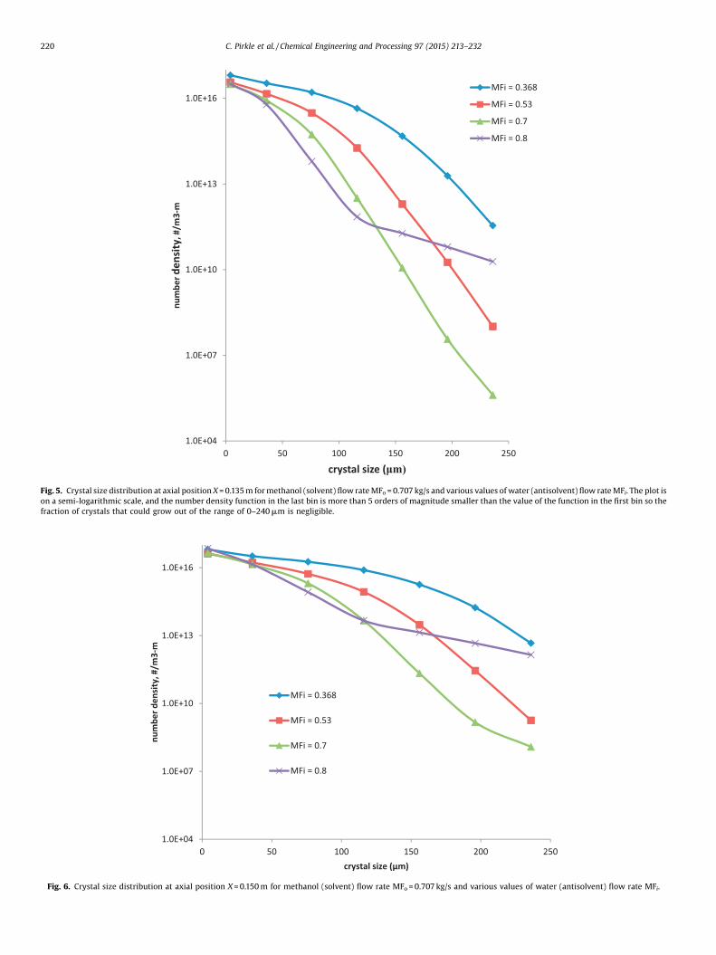
Fig. 6. Crystal size distribution at axial position X = 0.150 m for methanol (solvent) flow rate MFo= 0.707 kg/s and various values of water (antisolvent) flow rate MFi.

220 C. Pirkle et al. / Chemical Engineering and Processing 97 (2015) 213–232

Table 4Conditions for variable total mass flow rate.

Methanol mass flow (kg/s) Water mass flow(kg/s)

Residence time in mixing zone (s) Maximum turbulence Reynolds number % Solutecrystallized atX = 0.1 m

0.536 0.53 0.767 14152 79.470.707 0.70 0.581 18414 77.780.909 0.90 0.452 23947 76.93

Fig. 7. Local turbulent Reynolds number in coaxial nozzle at steady state for different total mass input rates (outer inlet: methanol saturated with lovastatin, inner inlet:water, water to methanol ratio = 0.99). Upper boundary (outer wall). Lower boundary (nozzle axis). Nozzle radius = 0.01816 m, Nozzle length = 1.0 m.

Fig. 8. Mean mixture fraction jh i3 in coaxial nozzle at steady state for different total mass input rates (outer inlet: methanol saturated with lovastatin, inner inlet:water, water to methanol ratio = 0.99). Upper boundary (outer wall). Lower boundary (nozzle axis). Nozzle radius = 0.01816 m, Nozzle length = 1.0 m.

C. Pirkle et al. / Chemical Engineering and Processing 97 (2015) 213–232 221

important variables in Figs. 7–17. For purposes of illustration, the Y(or transverse) dimension has been expanded by a factor of 5 inorder to make the contours more visible to the reader. Also, as thesystem is axisymmetric, only half of the mixer is shown. The centerline of the mixer (Y = 0) is the lower boundary, and the mixer wall

(Y = 0.01816 m) is the upper boundary. The axial length of the mixeris 1.0 m, but the entrance zone for the unmixed streams is 0.1 m,leaving 0.9 m for actual mixing. To compare the effect of input massflow rate, results for two inlet conditions are shown. Theseconditions are: inner mass flow rate = 0.53 kg/s, annular mass flow

Fig. 9. Volume fraction p3 of the mixed environment in coaxial nozzle at steady state for different total mass input rates (outer inlet: methanol saturated with lovastatin, innerinlet: water, water to methanol ratio = 0.99). Upper boundary (outer wall). Lower boundary (nozzle axis). Nozzle radius = 0.01816 m, Nozzle length = 1.0 m.

222 C. Pirkle et al. / Chemical Engineering and Processing 97 (2015) 213–232

rate = 0.536 kg/s; and inner mass flow rate = 0.90 kg/s, annularmass flow rate = 0.909 kg/s. These two sets of flow rates, with aconstant ratio of antisolvent to solvent flow of 0.99, correspond tototal residence times in the mixing zone of the coaxial nozzle of0.767 and 0.452 s, respectively. Thus, any axial position in a contourplot for the higher flow rate will correspond to a shorter residencetime than the same axial position for the lower flow rate. In orderto compare the coaxial nozzle results to the impinging jetcalculations of Woo et al. [40], which involved short residencetimes, key variables were sampled at locations just downstream ofthe mixing junction in the nozzle. The shorter residence timescorresponding to these locations are in the range of those used forthe impinging jet mixer.

Fig. 10. Solute concentration c, (kg/kg solvents), in coaxial nozzle at steady state for diffinlet: water, water to methanol ratio = 0.99). Upper boundary (outer wall). Lower boun

5.2. Mixing

The local turbulent Reynolds number in the coaxial nozzle isshown in Fig. 7, which has the same qualitative trend as impingingjet calculations [40,65,66]. As expected, the magnitude ofturbulence increases with input mass flow, maximizing at aboutX = 0.21 m and Y = 0.0 m in both cases. As the length of the innertube is 0.101 m, X = 0.21 m corresponds to a mixing length of0.109 m and residence times of 0.092 and 0.054 s, respectively, forthe lower and higher mass flow rates. As expected, turbulence isminimal at the tube wall, due to the no-slip condition.

As in the case of impinging jets, micro-mixing of the two inputfluids is rapid. As the mixed fluid, Environment 3, begins to form atthe junction of the inner and outer fluids, the fraction jh i3 of the

erent total mass input rates (outer inlet: methanol saturated with lovastatin, innerdary (nozzle axis). Nozzle radius = 0.01816 m, Nozzle length = 1.0 m.

Fig. 11. Antisolvent concentration as (kg/m33) within environment 3 in coaxial nozzle at steady state for different total mass input rates (outer inlet: methanol saturated with

lovastatin, inner inlet: water, water to methanol ratio = 0.99). Upper boundary (outer wall). Lower boundary (nozzle axis). Nozzle radius = 0.01816 m, Nozzle length = 1.0 m.

C. Pirkle et al. / Chemical Engineering and Processing 97 (2015) 213–232 223

mixed fluid that is formed from Environment 1 is higher in theouter region of the nozzle, as expected (see Fig. 8). For the higherinput flow conditions, the mixing is faster and more extensive,requiring a mixing time of only 0.085 s to achieve the completelymixed value (called the stoichiometric value) of jh i3 ¼ 0:51, ascompared to the 0.112 s required in the low flow case. In either case,less than 0.194 m (or a fifth) of the mixing zone is required forcomplete mixing.

As shown in Fig. 9, the volume fraction p3 of the mixedenvironment, mass-averaged over the cross-section, reaches0.95 at X = 0.31 m for the low input flow case, which correspondsto a residence time of 0.173 s. For the high input flow rate, theresidence time required to achieve a mass-based cross-sectionalaverage of 0.95 for p3 (at X = 0.41 m) is only 0.155 s, thus showingthat increased turbulence enhances micro-mixing.

Fig.12. Saturated solute concentration c* (kg/kg solvents) in coaxial nozzle at steady stateinner inlet: water, water to methanol ratio = 0.99). Upper boundary (outer wall). Lower

5.3. Crystallization dynamics

As shown in Fig. 10, the solute concentration c declines morequickly down the crystallizer for the lesser flow case than thehigher flow case, which is expected because the residence time ishigher for the former condition. The antisolvent concentration ispresented in Fig. 11, while contours for the saturated soluteconcentration c* are illustrated in Fig. 12. Just downstream of thejunction of the two inlets, the antisolvent (Environment 2) issufficiently mixed with the solution (Environment 1), so c* dropsby an order of magnitude, in agreement with Eq. (22). The relativesupersaturation S, shown in Fig. 13, has a contour pattern that isobviously correlated with antisolvent concentration, as does thenucleation rate B (Fig. 14), and the crystal growth rate G (Fig. 15).The latter two correlations are expected due to Eqs. (24) and (25).

for different total mass input rates (outer inlet: methanol saturated with lovastatin, boundary (nozzle axis). Nozzle radius = 0.01816 m, Nozzle length = 1.0 m.

Fig. 13. Supersaturation S (= c/c*) in the coaxial nozzle at steady state for different total mass input rates (outer inlet: methanol saturated with lovastatin, inner inlet: water,water to methanol ratio = 0.99). Upper boundary (outer wall). Lower boundary (nozzle axis). Nozzle radius = 0.01816 m, Nozzle length = 1.0 m.

224 C. Pirkle et al. / Chemical Engineering and Processing 97 (2015) 213–232

All these variables reach their maxima on the nozzle axis (center),and slightly downstream of the mixing junction. At the higherinput mass flow rate, the equivalent residence times are greater atany given axial location X; thus, the maximal regions of B and G aremore spread out spatially.

The total mass density of crystalsPj¼Ncell

j¼1 f w;j is shown in Fig. 16.

Not surprisingly, the distance required to achieve a total massdensity of 24 kg/m3 is larger for the higher input rate. As indicatedin Table 4, only 76.9–79.5% of crystallization is accomplishedwithin X = 1.0 m. In order to achieve more complete crystallization,it is obvious that the nozzle length will need to be increased toprovide more residence time, or the nozzle output should bedischarged into a holding tank.

Fig. 14. Nucleation rate B (#/s m3) in the coaxial nozzle at steady state for different total

water to methanol ratio = 0.99). Upper boundary (outer wall). Lower boundary (nozzle

5.4. Temperature and heats of mixing and crystallization

Temperature contours for the two total flow rates are comparedin Fig. 17. Other than turbulent diffusion, three major phenomenaare responsible for the spatial variation in temperature: (1) mixingof warmer and colder fluids entering the mixing tube; (2) heat ofmixing due to disruption of H2O–H2O intermolecular forces byintruding CH3OH molecules; and (3) heat released by crystalliza-tion of lovastatin from the methanol–water mixture.

Recall that the entrance temperature of the solute-containingfluid is 305 K, while that of the antisolvent-containing fluid is293 K. As the two input fluids mix, the solute is exposed not only toantisolvent but to a lower temperature as well. Both effects lowersolubility of the solute. Heats of mixing and crystallization negate

mass input rates (outer inlet: methanol saturated with lovastatin, inner inlet: water, axis). Nozzle radius = 0.01816 m, Nozzle length = 1.0 m.

Fig. 15. Crystal growth rate G (mm/s) in the coaxial nozzle at steady state for different total mass input rates (outer inlet: methanol saturated with lovastatin, inner inlet:water, water to methanol ratio = 0.99). Upper boundary (outer wall). Lower boundary (nozzle axis). Nozzle radius = 0.01816 m, Nozzle length = 1.0 m.

C. Pirkle et al. / Chemical Engineering and Processing 97 (2015) 213–232 225

some of the lowering of solubility by slightly increasing tempera-ture in Environment 3. The maximum increase of temperature dueto the mixing of methanol with water is 6.5 K, while that due to theheat of crystallization is 0.8 K.

As shown in Fig. 17, a higher maximum temperature occurs forthe higher flow rate, which can be attributed to the greater deliveryof solute, solvent and antisolvent per unit volume. In both cases,however, the region of maximum temperature is small. This resultsfrom the rapid turbulent dispersion of heat near this region whichlimits the effective temperature rise. At the point of initial mixing(X = 0.1 m), the heat of mixing increases the temperature ofEnvironment 3 to just under 309 K. Further equilibration bymixing drops the temperature to 304 K at X = 0.2 m.

Fig. 16. Total mass density of crystalsPj¼Ncell

j¼1 f w;jin the coaxial nozzle at steady stalovastatin, inner inlet: water, water to methanol ratio = 0.99). Upper boundary (length = 1.0 m.

5.5. Effect of mass input rate on crystal size distribution

For three total mass input flow rates, all with an antisolvent tosolvent flow ratio of 0.99, Figs. 18–22 show the cross-sectionallyaveraged crystal size distribution (CSD) at axial locations X = 0.12,0.135, and 0.15 m, respectively, within the coaxial nozzle. Themonotonically decreasing shape of the CSD resembles that of thesimulations by Woo et al. [39] and also the experimental CSD ofMahajan and Kirwan [2] for an unconfined impinging jet. Thelower the mass throughput, the longer is the residence timeavailable for nucleation and crystal growth. Thus, CSD increases inbreadth and magnitude as mass input rates decrease. Of course,crystal enlargement proceeds as the fluid mixture travels throughthe nozzle. As the axial location increases, the difference in CSD

te for different total mass input rates (outer inlet: methanol saturated withouter wall). Lower boundary (nozzle axis). Nozzle radius = 0.01816 m, Nozzle

Fig. 17. Temperature T (K) in coaxial nozzle at steady state for different total mass input rates (outer inlet: methanol saturated with lovastatin, inner inlet: water, water tomethanol ratio = 0.99). Upper boundary (outer wall). Lower boundary (nozzle axis). Nozzle radius = 0.01816 m, Nozzle length = 1.0 m.

226 C. Pirkle et al. / Chemical Engineering and Processing 97 (2015) 213–232

with respect to input flow rate becomes less discernible, especiallyfor lower crystal sizes.

Figs. 21 and 22 compare the crystal size distributions for variousthroughputs for fixed residence times of 0.01 and 0.02, respec-tively, which clearly show how an increase in residence timebroadens the CSD. Also, even at the same residence time, thehigher throughputs yield a sharper CSD, which agrees withexperiments in unconfined impinging jets [2]. Table 4 shows thatthe percentage of solute converted to crystals declines only slightlywith throughput, in spite of much lower residence times, which isdue to the increased turbulent mixing of antisolvent with solvent.

Fig. 18. Crystal size distribution at axial position X = 0.120 m for water (antisolven

6. Effect of mixer diameter upon crystallization

Turbulent transport properties could be affected by increasingthe mixer diameter, all other conditions being equal. By holdinginput mass fluxes (in kg/m2 s) constant and increasing the mixerdiameter 10 and 20 percent from the base-case diameter0.03632 m, calculations were made to determine the effect ofthe transverse dimensions on crystallization. That is, how adequateis transport in the radial direction. Table 5 shows the mixerparameters and the resulting crystallization percentage. Crystalsize distributions corresponding to the three diameters are plottedin Figs. 23 and 24 for X = 0.12 m and X = 1.0 m, respectively.

t) to methanol (solvent) flow ratio of 0.99 and various total mass flow rates.

Fig. 19. Crystal size distribution at axial position X = 0.135 m for water (antisolvent) to methanol (solvent) flow ratio of 0.99 and various total mass flow rates.

C. Pirkle et al. / Chemical Engineering and Processing 97 (2015) 213–232 227

Although there is some difference in CSD with respect to mixerdiameter at X = 0.12 m, there is little difference at X 1.0 m. For theflow conditions in Table 5, the results indicate that the turbulenttransport parameters responsible for transport in the transversedirection are sufficiently high to overcome the effect of transportdistances in the diameter range 3.6320–4.3584 cm.

Fig. 20. Crystal size distribution at axial position X = 0.150 m for water (antisolven

7. Summary and conclusions

The results in this paper on the simulation of mixing andcrystallization within a coaxial mixer are:

1. A simulation algorithm that couples macromixing and micro-mixing models with the solution to the full spatially-varyingpopulation balance equation (PBE) was implemented for a

t) to methanol (solvent) flow ratio of 0.99 and various total mass flow rates.

Fig. 21. Crystal size distribution at axial position tres = 0.01 s for water (antisolvent) to methanol (solvent) flow ratio of 0.99 and various total mass flow rates.

228 C. Pirkle et al. / Chemical Engineering and Processing 97 (2015) 213–232

coaxial mixer via a Fluent user-defined function (UDF) file. TheCFD-micromixing-PBE model computes the crystal size distri-bution throughout the crystallizer while taking into account thedifferent mixing time and length scales. Crystal nucleation,growth, and dissolution kinetics were included in the model. Anenergy equation was incorporated to compute the temperatureat every location and time in the mixer.

2. The UDF file was designed so that the user can readily replacethe model parameters, including physical properties for

Fig. 22. Crystal size distribution at axial position tres = 0.02 s for water (antisolven

antisolvent and solvent components. In the simulation resultspresented in this paper, the solvent was methanol and theantisolvent was liquid water.

3. Steady-state simulations were carried out by integrating thetransient model equations until all of the variables converged totheir steady-state values. Appropriate settings were found for theFluent SETUP code that enabled stable and accurate calculations.

4. Simulation results were presented for the application of theCFD-micromixing-PBE code to antisolvent crystallization within

t) to methanol (solvent) flow ratio of 0.99 and various total mass flow rates.

Table 5Effect of mixer diameter on crystallization.

Base diameter case 10% Larger diameter case 20% Larger diameter case

Mixer length, m 1 1 1Mixer diameter, cm 3.6320 3.9952 4.3584Annular mass flux, kg/m2 s 829 829 829Inner mass flux, kg/m2 s 11626 11626 11626Annular hydraulic diameter, m 0.021079 0.023186 0.025294Inner hydraulic diameter, m 0.008756 0.009631 0.010507Annular turbulent intensity, % 4.379 4.327 4.280Inner turbulent intensity, % 3.787 3.742 3.702Percentage soluteCrystallized at X = 1.0 m

77.78 77.58 77.36

Fig. 23. Crystal size distribution at axial position X = 0.120 m for water (antisolvent) to methanol (solvent) flow ratio of 0.99, annular mass flux = 829 kg/m2 s, inner massflux = 11626 kg/m2 s, and various mixing nozzle diameters.

Fig. 24. Crystal size distribution at axial position X = 1.0 m for water (antisolvent) to methanol (solvent) flow ratio of 0.99, annular mass flux = 829 kg/m2 s, inner massflux = 11626 kg/m2 s, and various mixing nozzle diameters.

C. Pirkle et al. / Chemical Engineering and Processing 97 (2015) 213–232 229

230 C. Pirkle et al. / Chemical Engineering and Processing 97 (2015) 213–232

a coaxial nozzle mixer. The model used solubility andcrystallization kinetics for lovastatin that were available inthe literature.

5. The simulations indicated the effect that operating conditionshad upon total crystallization and crystal size distribution.

This detailed simulation of coaxial crystallizers parallels thatdone for impinging jet crystallizers. The results demonstrate thepossibility of influencing crystal size distribution by adjustingoperating conditions (such as inlet stream velocities) of the coaxialcrystallizer. Such simulations can facilitate development in thepharmaceutical industry by providing a more insight into thecrystallization process, and by reducing the number of experi-ments required to determine optimal operating conditions. This, inturn, reduces the quantity of active pharmaceutical ingredient(API) needed for the experiments. Consequently, the crystallizerprocess design can be performed much earlier during the drugdevelopment process, where a limited quantity of API is available.

Acknowledgements

Financial support from Pfizer, Inc. is acknowledged.

Appendix A.

NomenclatureAc Crystal surface area (m2)

asj Concentration of antisolvent j in Environment 3ðkg=m33Þ

b Nucleation rate exponentB Nucleation rate (#/m3 s)c Concentration of solute (kg/m3 or kg/kg)c* Solubility or saturation concentration (kg/m3 or kg/kg)Dc Supersaturation (kg/m3 or kg/kg)ci Interfacial concentration (kg/m3)Cp,3 Specific heat of Environment 3, kJ/kgCm Constant in turbulent viscosity expressionD,Dm Diffusion coefficient or laminar diffusivity (m2/s)dp Particle size (mc)Dt Turbulent diffusivity (m2/s)f Number density function (#/mcm3)F Target number density function (#/m)fr Derivative of number density function (#/mc

2m3)fw Mass density function (kg/mcm3)f’ Joint probability function of all scalarsg Growth rate exponent~g Gravitational acceleration (m/s2)G Growth rate (m/s)G(p) Rate of change of p = (p1 p2 � � � pNe) due to micromixingGs(p) Term to eliminate spurious dissipation rate in Eq. (12)h Enthalpy per unit volume, kJ/m3

i Exponent for solute integrationk Turbulent kinetic energy (m2/s2) in turbulence and

micromixing equations and Boltzmann’s constant innucleation rate expression

K Tradeoff ratio between growth and nucleation rates((mm/s)/(#/m3 s))

k1, k2 Reaction rate constant (m3/mol s)kb Nucleation rate prefactor (#/m3 s (kg/kg)b)ka Area shape factorkd Mass transfer coefficient (m/s)kg Growth rate prefactor (m/s (kg/kg)g)ki Integration rate constant (m3i�1/kgi�1 s)kv Volume shape factorL Crystal size (mm)

Mn Rate of change of sh in due to micromixingMn

s Term to eliminate spurious dissipation rate in Eq. (13)m Mass (kg)_m Mass flow rate (kg/s)MWH2O Molecular weight of water, kg/kmolMWsolute Molecular weight of solute, kg/kmolNA Avogadro’s numberN Number of particle size cells or binsNe Number of probability modes or environmentsNs Total number of scalars (species)p Pressure (Pa) in momentum conservation equationpn Probability of mode n or volume fraction of Environment

n in micromixing modelr Crystal size (m)r0 Nuclei size (m)Dr Discretized bin size for crystal size (m)Re Reynolds numbersh in Weighted concentration of mean composition of scalars

w in mode nS Relative supersaturation = Dc/c*Sas User-defined source term of antisolvent concentration

(kg/m3 s)Sfw,j User-defined source term of crystal mass density in the

jth bin (kg/mcm3 s)Ss User-defined source term of solvent concentration (kg/

m3 s)Se User-defined source term for dissipation rate of turbu-

lent kinetic energySk User-defined source term for turbulent kinetic energySc Schmidt numberSct Turbulent Schmidt numberSh Sherwood numbert Time (s)T Temperature (C)tI Induction time (s)tM Micromixing time (s)ts Sampling time (s)v Molar volume in nucleation rate expression (m3/mol)V Velocity vector (m/s)V Volume fraction of antisolventw Antisolvent mass percent (%)x Spatial position vector (m)X Reaction conversionXA Fraction of polymorph A

Special unitsm Length unit (meter) in mixer/crystallizermc Length unit (meter) in crystalm3 Length unit (meter) in Environment 3

Symbolsa Scalarb Geometric shape factorDc supersaturation = c – c*e Turbulent kinetic energy dissipation rate (m2/s3)ej Scalar dissipation rate (1/s)f Volume fraction of solids in an effective viscosity expressionfk Scalarfh i Mean composition of a scalar in an environmentr3 Fluid density of Environment 3g Interfacial tension [N/m]lk Kolmogoroff length scalem Viscosity (kg/m s) effective viscosity of suspension (kg/m s)

in effective viscosity expression

C. Pirkle et al. / Chemical Engineering and Processing 97 (2015) 213–232 231

mn nth moment of number density functionms Viscosity of suspending medium (kg/m s)mt Viscosity (kg/m s)u Constant in minmod limiteruj Parameter valuer Density (kg/m3)rc Crystal density (kg/m3)se Turbulent Prandtl number for turbulent kinetic energy

dissipation ratesk Turbulent Prandtl number for turbulent kinetic energyt Stress tensor (kg/m s2)n Kinematic viscosity (m2/s)jh i Mixture fractionj02�

Mixture fraction variancec A dummy variableca An element of c corresponding to the scalar a

Subscriptsi Crystal dimension in population balance equation Instance for

dropping seed crystalsc Denotes crystal propertyj Discretized bin for crystal size in population balance equationn Environment in micromixing model Order of moment

Appendix B.

High-Resolution, Finite-Volume, Semidiscrete Central Schemes

High-resolution finite-volume methods have been investigatedprimarily in the applied mathematics and computational physicsliterature [52]. These methods provide high accuracy for simulat-ing hyperbolic conservation laws while reducing numericaldiffusion and eliminating nonphysical oscillations that can occurwith classical methods. Being in the class of finite volume methods,such methods are conservative, which ensures the accuratetracking of discontinuities and preserves the total mass withinthe computational domain subject to the applied boundaryconditions. Another advantage is that these numerical schemescan be easily extended to solve multidimensional and variable-coefficient conservation laws.

High-resolution central schemes for nonlinear conservationlaws, starting from the NT scheme of Nessyahu and Tadmor [62],have the advantages of retaining the simplicity of the Riemann-solver-free approach, while achieving at least second-orderaccuracy. Kurganov and Tadmor [63] and Kurganov et al. [64]extended the NT scheme to reduce numerical viscosity (nonphysi-cal smoothing of the numerical solution) arising from discreteapproximations of the advection term. This KT high-resolutionfinite-volume central scheme accumulates less dissipation for afixed Dy as compared to the NT scheme, and can be used efficientlywith small time steps since the numerical viscosity is independentof (1/Dt). The limiting case, Dt ! 0, results in the second-ordersemidiscrete version. In addition, the KT method satisfies the scalartotal-variation-diminishing (TVD) property with minmod recon-struction, which implies that the nonphysical oscillations thatoccur with many second-order accurate numerical methodscannot occur with this method. The KT semidiscrete scheme isparticularly effective when combined with high-order ODE solversfor the time evolution.

Consider the nonlinear conservation law,

@@uðy; tÞ þ @

@yqðuðy; tÞÞ ¼ 0 (B.1)

The semidiscrete central scheme of Kurganov and Tadmor [63]is classified as a finite-volume method, since it involves keepingtrack of the integral of u over each grid cell. The use of cell averages,

ujðtÞ ¼ 1Dy

Z yjþ1=2

yj�1=2

uðy; tÞdy; (B.2)

to represent computed values, where Dy ¼ yjþ1=2 � yj�1=2, ensuresthat the numerical method is conservative. The second-ordersemidiscrete scheme admits the conservative form:

ddtujðtÞ ¼ �Hjþ1=2ðtÞ � Hj�1=2ðtÞ

Dy(B.3)

with the numerical flux

Hjþ1=2ðtÞ :

¼qðuþ

jþ1=2ðtÞÞ þ qðuþjþ1=2ðtÞÞ

2� ajþ1=2

2½uþ

jþ1=2ðtÞ � u�jþ1=2ðtÞ� (B.4)

and the intermediate values given by

uþjþ1=2 :¼ ðujþ1=2ðtÞ �Dy

2ðuyÞjþ1ðtÞ

uþjþ1=2 :¼ ðujðtÞ �Dy

2ðuyÞjðtÞ

while the local propagation of speeds, for the scalar case, is

ajþ1=2ðtÞ :¼ maxu2½u�

jþ1=2ðtÞ;uþjþy2ðtÞ�

jq0ðu�jþ1=2ðtÞÞj (B.6)

The derivatives are approximated with the minmod limiter:

ðuyÞnj :¼ minmond uunj � un

j�1

Dy;unjþ1 � un

j�1

2Dy;unjþ1 � un

j

Dy

!1�u�2

(B.7)

which is defined as

minmondða1; a2; . . .Þ ¼

minfaigimaxfaigi

ifai > 08iifai > 08i

0 otherwise

8>>>>>><>>>>>>:

(B.8)

Selecting the value of u = 1 results in nonphysical smoothing of thenumerical solution. A value of u = 2 results in minimal nonphysicalsmoothing, but can introduce some nonphysical oscillation. Thevalue u = 1.5 is commonly selected to trade off minimizing theamount of nonphysical dissipation/smoothing with minimizingnonphysical oscillation. More details on such limiters can be foundin the above References

References

[1] M.D. Lindrud, S. Kim, C. Wei, U.S. Patent #6302958, 2001.[2] A.J. Mahajan, D.J. Kirwan, AIChE J. 42 (1996) 1801–1814.[3] M. Midler, E.L. Paul, E.F. Whittington, M. Futran, P.D. Liu, J. Hsu, S.-H. Pan U.S.

Patent #5314506, 1994.[4] D.J. Am Ende, S.J. Brenek, Am. Pharm. Rev. 7 (2004) 98–104.[5] S.S. Leung, B.E. Padden, E.J. Munson, D.J.W. Grant, J. Pharm. Sci. 87 (1998) 501–

507.[6] J.W. Mullin, Crystallization, Elsevier Butterworth-Heineman, Oxford, U.K,

2001.[7] J.S. Wey, P.H. Karpinski, Batch crystallization, Handbook of Industrial

Crystallization, Butterworth-Heinemann, Boston, 2002231–248.[9] B.K. Johnson, R.K. Prud’homme, AIChE J. 49 (2003) 2264–2282.

[10] M. Fujiwara, Z.K. Nagy, J.W. Chew, R.D. Braatz, J. Process Control 15 (2005) 493–504.

[11] R. Dauer, J.E. Mokrauer, W.J. McKeel, U.S. Patent 5578279, 1996.[12] M.D. Lindrud, S. Kim, C. Wei, U.S. Patent 6302958, 2001.[13] D.J. Am Ende, T.C. Crawford, N.P. Weston, U.S. Patent 6558435, 2003.[14] X. Wang, J.M. Gillian, D.J. Kirwan, Cryst. Growth Des. 6 (2006) 2214–2227.

232 C. Pirkle et al. / Chemical Engineering and Processing 97 (2015) 213–232

[15] H. Wei, J. Garside, Chem. Eng. Res. Des. 75 (1995) 219–227.[16] J. Baldyga, W. Orciuch, Chem. Eng. Sci. 56 (2001) 2435–2444.[17] D.L. Marchisio, A.A. Barresi, M. Garbero, AIChE J. 48 (2001) 2039–2050.[18] A.A. Öncül, K. Sundmacher, A. Seidel-Morgenstern, D. Thévenin, Chem. Eng.

Sci. 61 (2006) 652–664.[19] A. Borissova, Z. Dashova, X. Lai, K.J. Roberts, Cryst. Growth Des. 4 (2004) 1053–

1060.[20] J. Budz, P.H. Karpinski, J. Mydlarz, J. Nyvlt, Ind. Eng. Chem. Prod. Res. Dev. 25

(1986) 657–664.[21] H. Charmolue, R.W. Rousseau, AIChE J. 37 (1991) 1121–1128.[22] N. Doki, N. Kubota, M. Yokota, S. Kimura, S. Sasaki, J. Chem. Eng. Jpn. 35 (2002)

1099–1104.[23] R.A. Granberg, D.G. Bloch, A.C. Rasmuson, J. Cryst. Growth 199 (1999) 1287–

1293.[24] X. Holmback, A.C. Rasmuson, J. Cryst. Growth 199 (1999) 780–788.[25] S. Kaneko, Y. Yamagami, H. Tochihara, I. Hirasawa, J. Chem. Eng. Jpn. 35 (2002)

1219–1223.[26] J.W. Mullin, N. Teodossiev, O. Sohnel, Chem. Eng. Process. 26 (1989) 93–99.[27] J. Mydlarz, A.G. Jones, Powder Technol. 65 (1991) 187–194.[28] J. Nyvlt, S. Zacek, Collect. Czech. Chem. Commun. 51 (1986) 1609–1617.[29] E. Plasari, P. Grisoni, J. Villermaux, Chem. Eng. Res. Des. 75 (1997) 237–244.[30] D.M. Shin, W.S. Kim, J. Chem. Eng. Jpn. 35 (2002) 1083–1090.[31] H. Takiyama, T. Otsuhata, M. Matsuoka, Chem. Eng. Res. Des. 76 (1998) 809–

814.[32] Y. Kim, S. Haam, Y.G. Shul, W.S. Kim, J.K. Jung, H.C. Eun, K.K. Koo, Ind. Eng.

Chem. Res. 42 (2003) 883–889.[33] M. Kitamura, J. Cryst. Growth 237 (2002) 2205–2214.[34] M. Kitamura, K. Nakamura, J. Chem. Eng. Jpn. 35 (2002) 1116–1122.[35] M. Kitamura, M.J. Sugimoto, Cryst. Growth 257 (2003) 177–184.[36] M. Okamoto, M. Hamano, H. Ooshima, J. Chem. Eng. Jpn. 37 (2004) 95–101.[37] J.W. Schroer, K.M. Ng, Ind. Eng. Chem. Res. 42 (2003) 2230–2244.[38] X.Y. Woo, R.B.H. Tan, P.S. Chow, R.D. Braatz, Cryst. Growth Des. 6 (2006) 1291–

1303.[39] X.Y. Woo, Modeling and simulation of antisolvent crystallization: mixing and

control, Ph.D. Thesis, University of Illinois, Urbana-Champaign, 2007.[40] X.Y. Woo, R.B.H. Tan, R.D. Braatz, Cryst. Growth Des. 9 (2009) 156–164.

[41] R.O. Fox, Computational Models for Turbulent Reacting Flows, CambridgeUniversity Press, Cambridge, U.K, 2003.

[42] A. Varma, M. Morbidelli, H. Wu, Parametric Sensitivity in Chemical Systems,Cambridge University Press, Cambridge, U.K, 1999.

[43] A.J. Mahajan, D.J. Kirwan, J. Cryst. Growth 144 (1994) 281–290.[44] S.B. Pope, Turbulent Flows, Cambridge University Press, Cambridge, U.K, 2000.[45] Fluent User’s Guide, ANSYS Fluent User’s Guide, Release 14.0. ANSYS, Inc.,

Canonsburg, Pennsylvania, 2011.[46] Ansys 14.5, www.ansys.com/Products/ANSYS 14.5 Release Highlights.[47] H.M. Hulburt, S. Katz, Chem. Eng. Sci. 19 (1964) 555–574.[48] A.D. Randolph, M.A. Larson, Theory of Particulate Processes, Academic Press,

Inc., San Diego, California, 1988.[49] R. Gunawan, I. Fusman, R.D. Braatz, AIChE J. 50 (2004) 2738–2749.[50] D.L. Ma, R.D. Braatz, D.K. Tafti, Int. J. Mod. Phys. B 16 (2002) 383–390.[51] D.L. Ma, D.K. Tafti, R.D. Braatz, Ind. Eng. Chem. Res. 41 (2002) 6217–6223.[52] D.L. Ma, D.K. Tafti, R.D. Braatz, Comput. Chem. Eng. 26 (2002) 1103–1116.[53] R.J. Leveque, Finite Volume Methods for Hyperbolic Problems, Cambridge

University Press, Cambridge, U.K, 2002.[54] L.G. Wang, R.O. Fox, AIChE J. 50 (2004) 2217–2232.[55] D.L. Marchisio, A.A. Barresi, R.O. Fox, AIChE J. 47 (2001) 664–676.[56] D.L. Marchisio, R.O. Fox, A.A. Barresi, G. Baldi, Ind. Eng. Chem. Res. 40 (2001)

5132–5139.[57] D.L. Marchisio, R.O. Fox, A.A. Barresi, M. Garbero, G. Baldi, Chem. Eng. Res. Des.

79 (2001) 998–1004.[58] D. Piton, R.O. Fox, B. Marcant, Can. J. Chem. Eng. 78 (2000) 983–993.[59] G.L. Bertrand, F.J. Millero, C.-H. Wu, L.G. Hepler, J. Phys. Chem. 70 (1966) 699–

705.[60] H.H. Tung, E.L. Paul, M. Midler, J.A. McCauley, Crystallization of Organic

Compounds: An Industrial Perspective, John Wiley & Sons, Hoboken, NewJersey, 2009.

[61] H. Sun, J.-B. Gong, J.-K. Wang, J. Chem. Eng. Data 56 (2006) 1389–1391.[62] A.J. Mahajan, D.J. Kirwan, AIChE J. 42 (1996) 1801–1814.[63] H. Nessyahu, E. Tadmor, J. Comput. Phys. 87 (1990) 408–463.[64] A. Kurganov, E. Tadmor, J. Comput. Phys. 160 (2000) 241–282.[65] A. Kurganov, S. Noelle, G. Petrova, SIAM J. Sci. Comput. 23 (2001) 707–740.[66] Y. Liu, R.O. Fox, AIChE J. 52 (2006) 731–744.