Modeling and Optimization of Next Generation Feedstock Development for Chemical Process 

Industry

Selen CremaschiSelen CremaschiDepartment of Chemical EngineeringThe University of Tulsa, Tulsa, OK, USA

Pan‐American Advanced Studies InstituteProcess Modeling and Optimization for Energy and SustainabilityProcess Modeling and Optimization for Energy and Sustainability

Angra dos Reis, RJ, BrazilJuly 19‐29, 2011

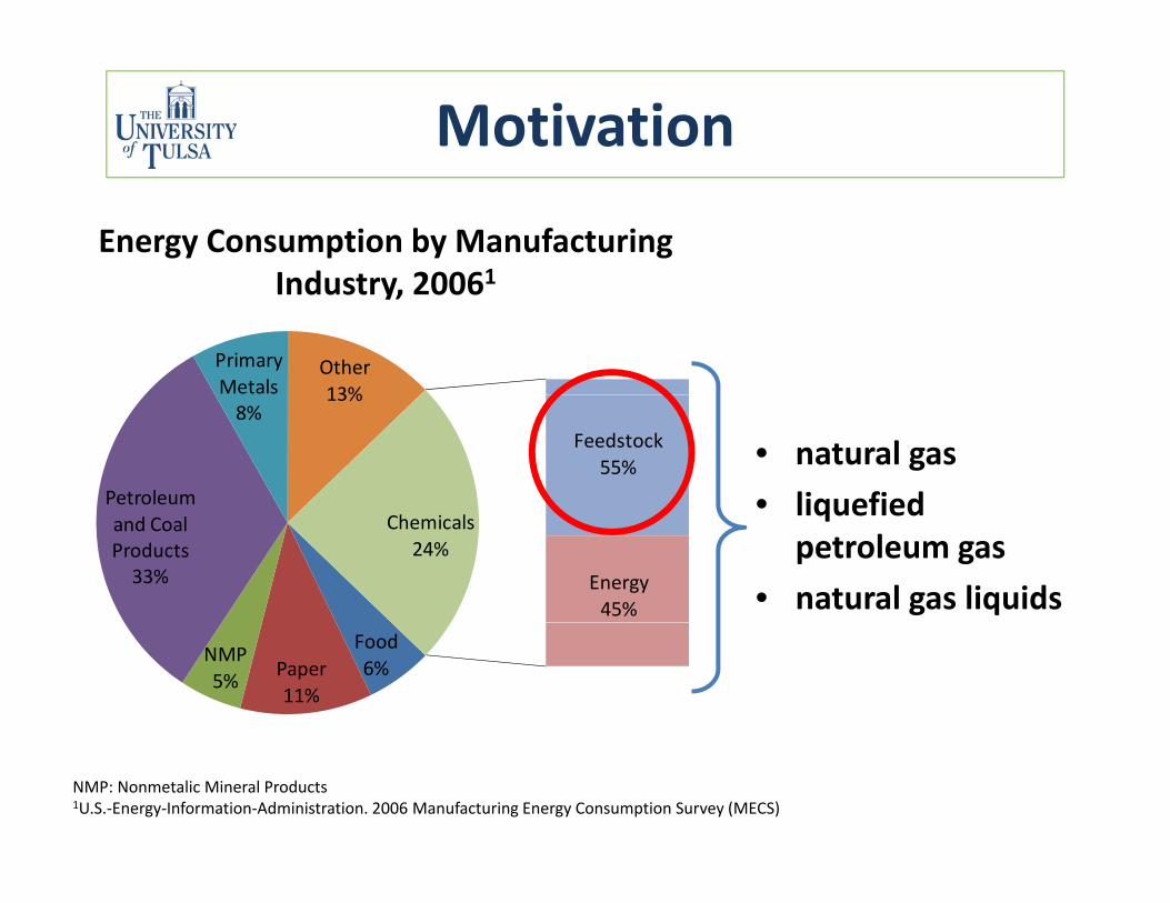
Motivation

Energy Consumption by Manufacturing Industry 20061Industry, 20061

Primary Metals

Other13%

Petroleum 

8%13%

Feedstock55% • natural gas

• liquefiedand Coal Products33% Energy

45%

Chemicals24%

liquefied petroleum gas

• natural gas liquidsFood6%Paper

11%

NMP5%

NMP: Nonmetalic Mineral Products1U.S.‐Energy‐Information‐Administration. 2006 Manufacturing Energy Consumption Survey (MECS)

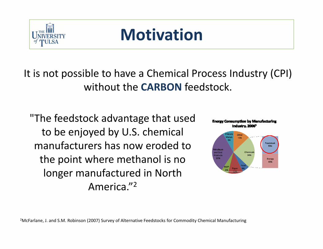
Motivation

It is not possible to have a Chemical Process Industry (CPI) p y ( )without the CARBON feedstock.

"The feedstock advantage that used to be enjoyed by U.S. chemical 

manufacturers has now eroded to the point where methanol is no longer manufactured in Northlonger manufactured in North 

America.”2

2McFarlane, J. and S.M. Robinson (2007) Survey of Alternative Feedstocks for Commodity Chemical Manufacturing

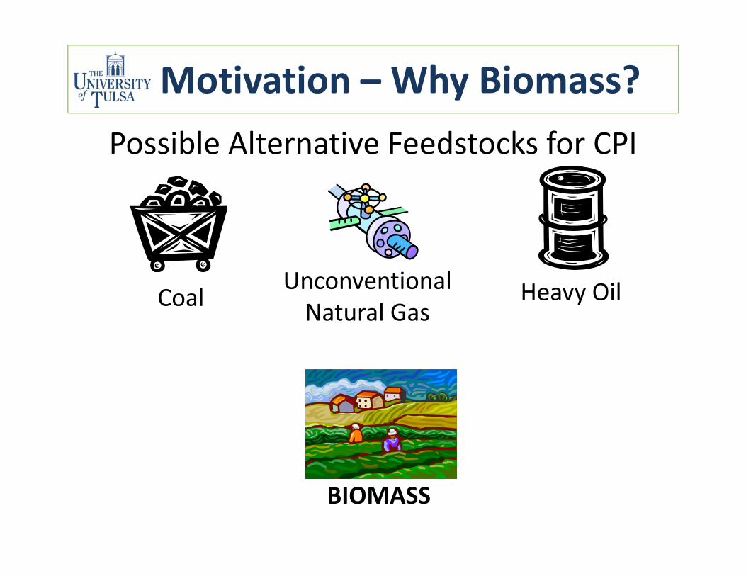
Motivation – Why Biomass?Possible Alternative Feedstocks for CPI

CoalUnconventional Natural Gas

Heavy Oil

BIOMASS

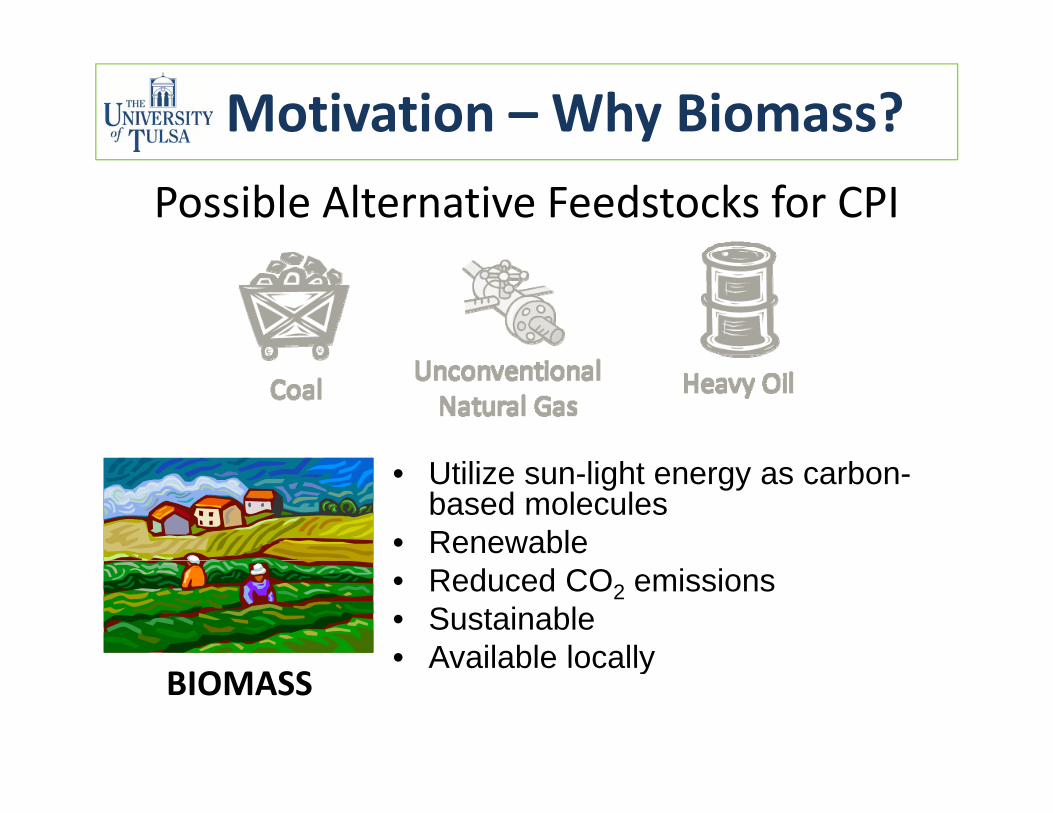
Motivation – Why Biomass?Possible Alternative Feedstocks for CPI

• Utilize sun-light energy as carbon-based molecules

• Renewable• Reduced CO2 emissions• Sustainable• Available locallyAvailable locally

BIOMASS

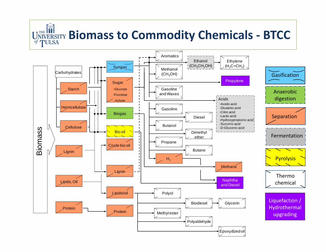
Biomass to Commodity Chemicals ‐ BTCC

CarbohydratesSyngas

Ethanol (CH3CH2OH)

Ethylene (H2C=CH2)Methanol

(CH3OH)

Aromatics

Gasification

Gasoline and Waxes

Starch

Hemicellulose

Sugar-Glucose

-Fructose

-Xylose

Propylene

Gasoline

Acids-Acetic acid-Glutamic acid

Anaerobic digestion

mas

s Cellulose

Biogas

Bio oil

Gasoline

Diesel

Butanol

Dimethyl ether

Propane

-Citric acid-Lactic acid-Hydroxypropionic acid-Succinic acid-D-Gluconic acid

Fermentation

Separation

Lignin

LigninBio

m Crude bio oil

H2

Methane

Propane

Butane

Pyrolysis

h

Lipids/oil

Lipids, Oil

Polyol

Biodiesel Glycerin

Naphtha and Diesel

Liquefaction / d h l

Thermo chemical

ProteinProtein

Methyl ester

Polyaldehyde

Epoxydized oil

Hydrothermal upgrading

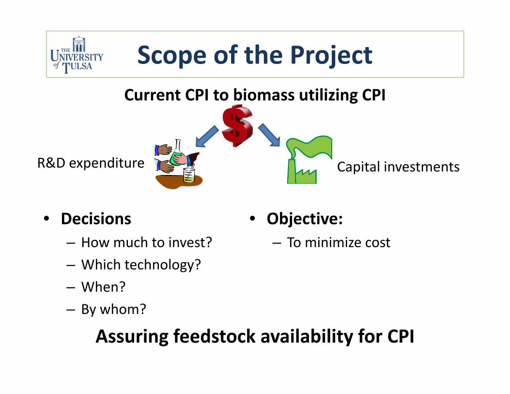
Scope of the ProjectCurrent CPI to biomass utilizing CPI

R&D expenditure Capital investments

• Decisions • Objective:

p

Decisions– How much to invest?– Which technology?

Objective:– To minimize cost

gy– When?– By whom?

Assuring feedstock availability for CPI

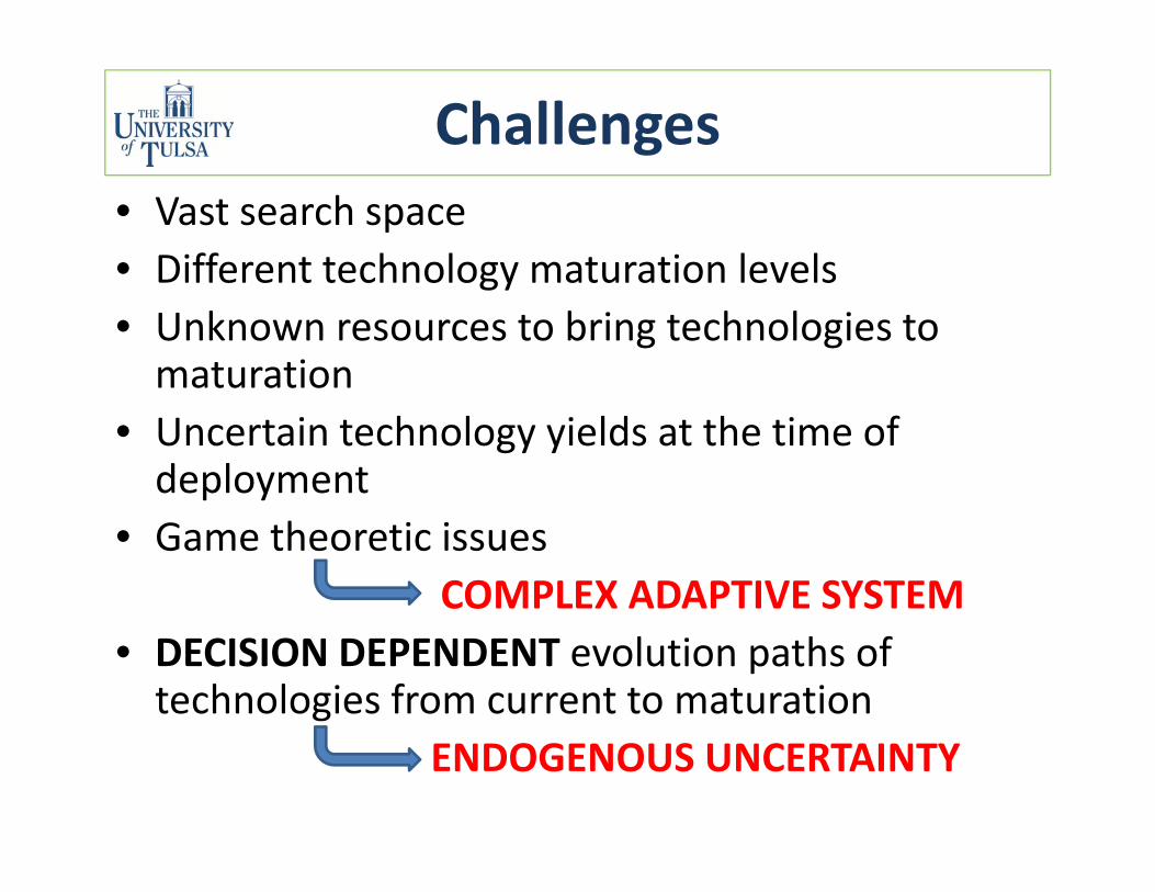
Challenges• Vast search space• Different technology maturation levelsDifferent technology maturation levels• Unknown resources to bring technologies to maturation

• Uncertain technology yields at the time of deployment

• Game theoretic issuesCOMPLEX ADAPTIVE SYSTEM

• DECISION DEPENDENT evolution paths of technologies from current to maturation

ENDOGENOUS UNCERTAINTY

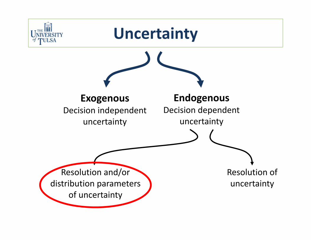
Uncertainty

Exogenous EndogenousDecision independent 

uncertaintyDecision dependent 

uncertainty

Resolution of uncertainty

Resolution and/or distribution parameters 

of uncertaintyof uncertainty

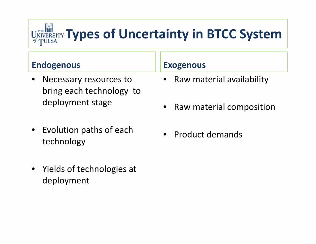
Types of Uncertainty in BTCC System

Endogenous Exogenousl l b l• Necessary resources to 

bring each technology  to deployment stage

• Raw material availability

• Raw material compositionp y g

• Evolution paths of each 

• Raw material composition

• Product demandstechnology

• Yields of technologies at

oduct de a ds

• Yields of technologies at deployment

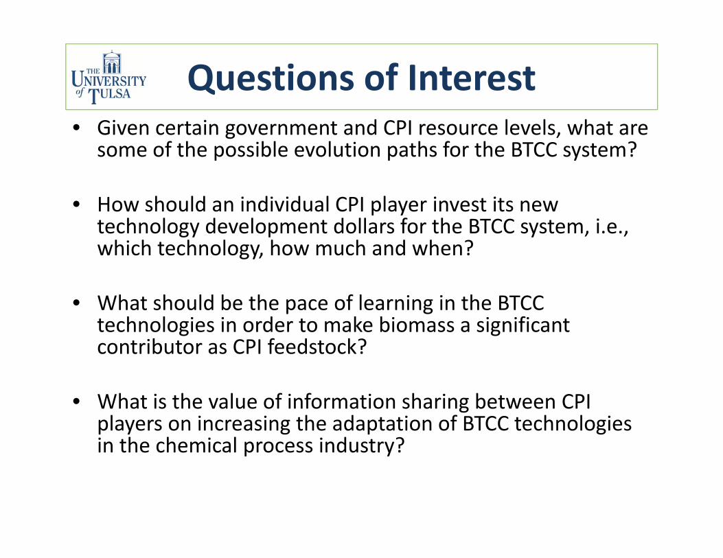
Questions of Interest• Given certain government and CPI resource levels, what are 

some of the possible evolution paths for the BTCC system?

• How should an individual CPI player invest its new technology development dollars for the BTCC system, i.e., hi h t h l h h d h ?which technology, how much and when?

• What should be the pace of learning in the BTCC technologies in order to make biomass a significant contributor as CPI feedstock?

• What is the value of information sharing between CPI players on increasing the adaptation of BTCC technologies in the chemical process industry?p y

How to Model the Problem?• Need a suitable framework

– To represent and model the BTCC investmentTo represent and model the BTCC investment problem

– That is easily scalable– That is universal, i.e., independent of the type of technology

– That is able to represent the uncertain evolution paths of different technologies and their dependence on the investment decisionsdependence on the investment decisions

– That is amenable to collaborative community upkeep and expansion.

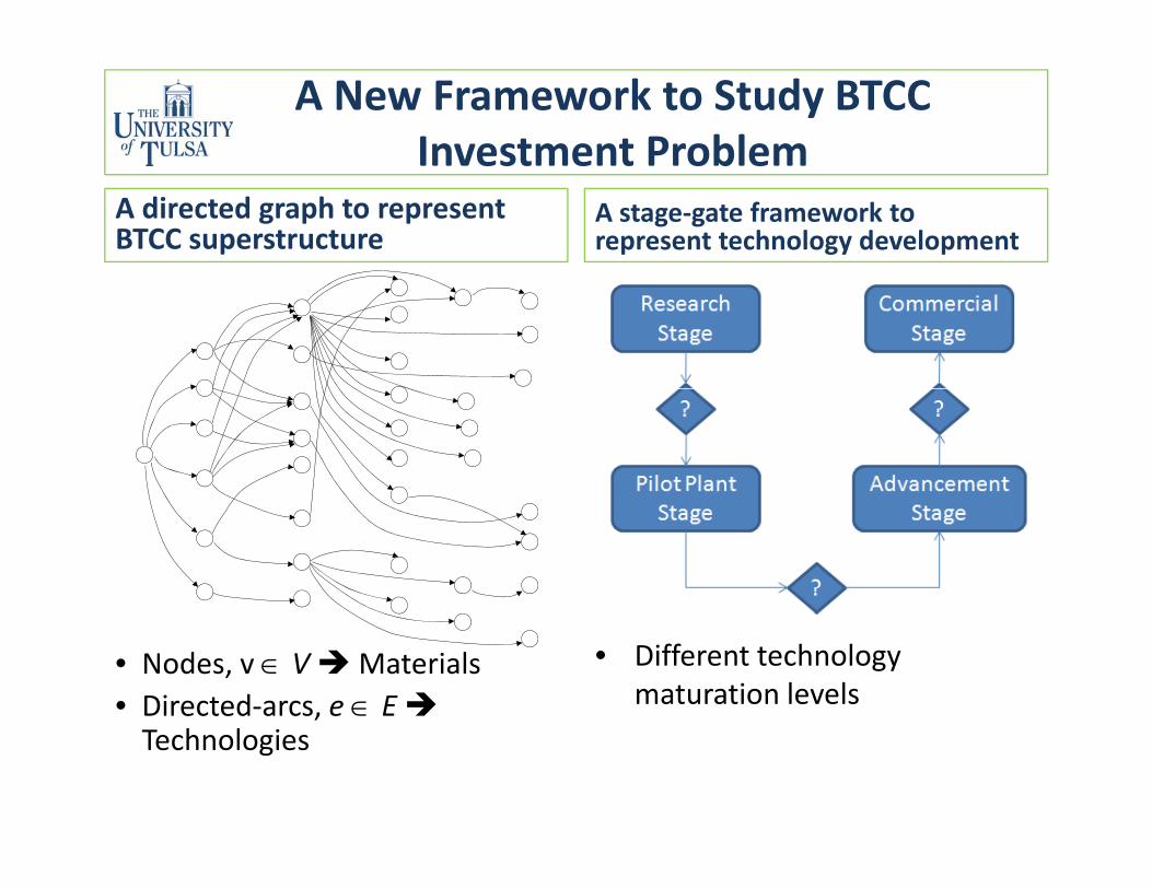
A New Framework to Study BTCC Investment ProblemInvestment Problem

A directed graph to represent BTCC superstructure

A stage‐gate framework to represent technology development

• Nodes, v VMaterials• Directed‐arcs, e E

• Different technology maturation levels

Technologies

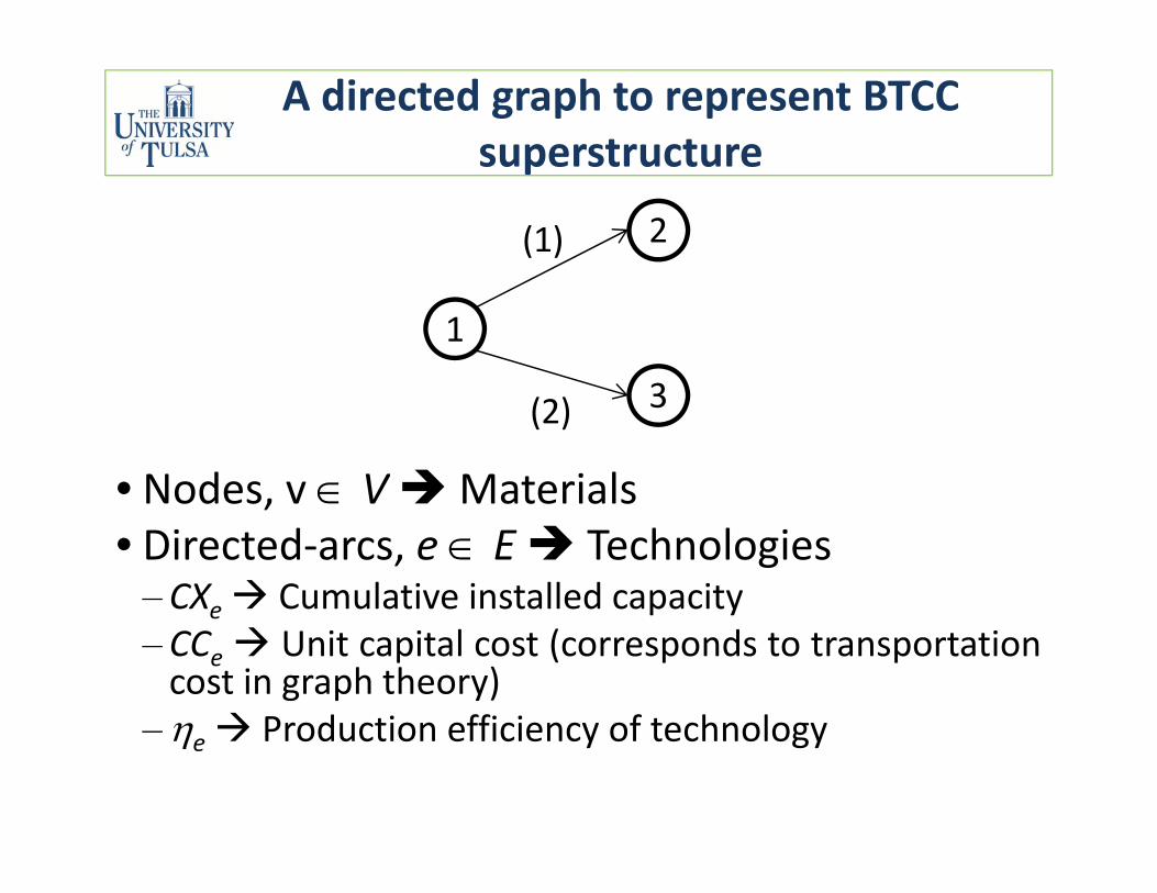
A directed graph to represent BTCC superstructuresuperstructure

2(1)

1

3

• Nodes, v VMaterials

3(2)

Nodes, v VMaterials• Directed‐arcs, e E Technologies‒ CXe Cumulative installed capacitye‒ CCe Unit capital cost (corresponds to transportationcost in graph theory) Production efficiency of technology‒e Production efficiency of technology

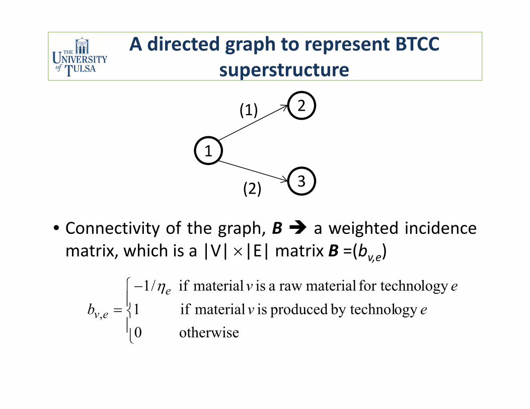
A directed graph to represent BTCC superstructuresuperstructure

2(1)

1

3

• Connectivity of the graph B a weighted incidence

3(2)

Connectivity of the graph, B a weighted incidencematrix, which is a |V| |E| matrix B =(bv,e)

lf t ht i lit i lif/1

otherwise0ogy by technol produced is material if 1

logy for technomaterialrawaismaterialif /1

, evev

be

ev

otherwise 0

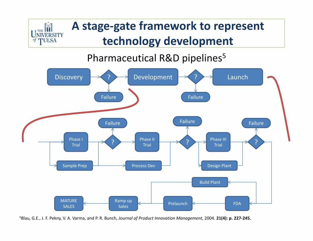
A stage‐gate framework to represent technology developmenttechnology development

Pharmaceutical R&D pipelines5

Di D l L h? ?Discovery Development Launch? ?

Failure Failure

Failure Failure Failure

Phase I Trial

Phase II Trial

Phase III Trial

Sample Prep Process Dev Design Plant

? ? ?

Sample Prep Process Dev Design Plant

Build Plant

5Blau, G.E., J. F. Pekny, V. A. Varma, and P. R. Bunch, Journal of Product Innovation Management, 2004. 21(4): p. 227‐245.

FDAPrelaunchRamp up Sales

MATURE SALES

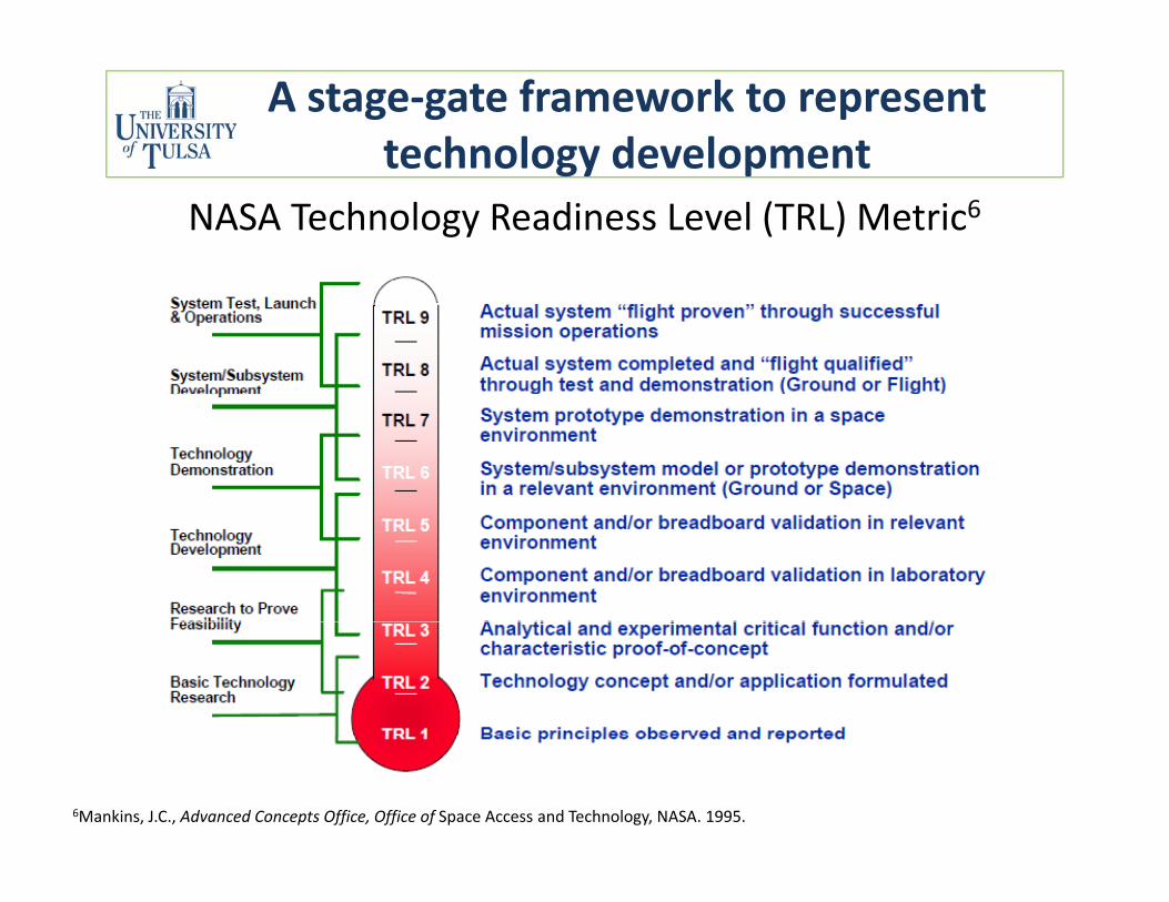
A stage‐gate framework to represent technology developmenttechnology development

NASA Technology Readiness Level (TRL) Metric6

6Mankins, J.C., Advanced Concepts Office, Office of Space Access and Technology, NASA. 1995.

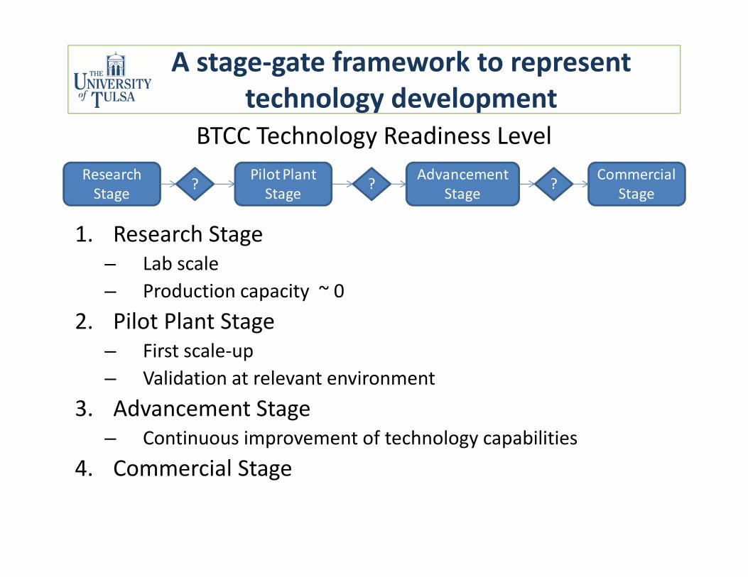
A stage‐gate framework to represent technology developmenttechnology development

BTCC Technology Readiness LevelResearch  Pilot Plant  Advancement  Commercial ? ? ?

1. Research Stage

Stage Stage Stage Stage? ? ?

– Lab scale– Production capacity  ~ 0

2 Pilot Plant Stage2. Pilot Plant Stage– First scale‐up– Validation at relevant environment

3. Advancement Stage– Continuous improvement of technology capabilities

4 Commercial Stage4. Commercial Stage

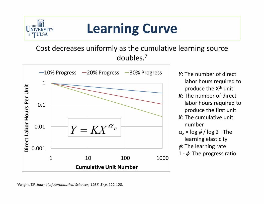
Learning CurveCost decreases uniformly as the cumulative learning source 

doubles.7

1

nit

10% Progress 20% Progress 30% Progress Y: The number of direct labor hours required to produce the Xth unit

0.1

ours Per Un produce the X unit

K: The number of direct labor hours required to produce the first unit

0.01

ct Lab

or Ho

eKXY X: The cumulative unit number

e = log  / log 2 : The learning elasticity

0.001

1 10 100 1000

Direc

Cumulative Unit Number

learning elasticity: The learning rate1 ‐ : The progress ratio

Cumulative Unit Number

7Wright, T.P. Journal of Aeronautical Sciences, 1936. 3: p. 122‐128.

Two‐Factor Learning Curve8

eett CRDCX

e

te

e

teete CRD

CRDCXCX

CCCC

0,

,

0,

,0,,

Learning‐by‐doing

Learning‐by‐searching

• CCe,t: Unit capital cost for technology e at time t• CXe,t: Cumulative installed capacity of technology e at time t• CRDe,t: Total R&D expenditure for technology e at time t• αe: Learning-by-doing elasticity for technology e• : Learning-by-searching elasticity for technology ee: Learning-by-searching elasticity for technology e

8Kouvaritakis, N., A. Soria, and S. Isoard, International Journal of Global Energy Issues 2000. 14(1‐4): p. 104‐115.

Modeling the BTCC Investment Problem

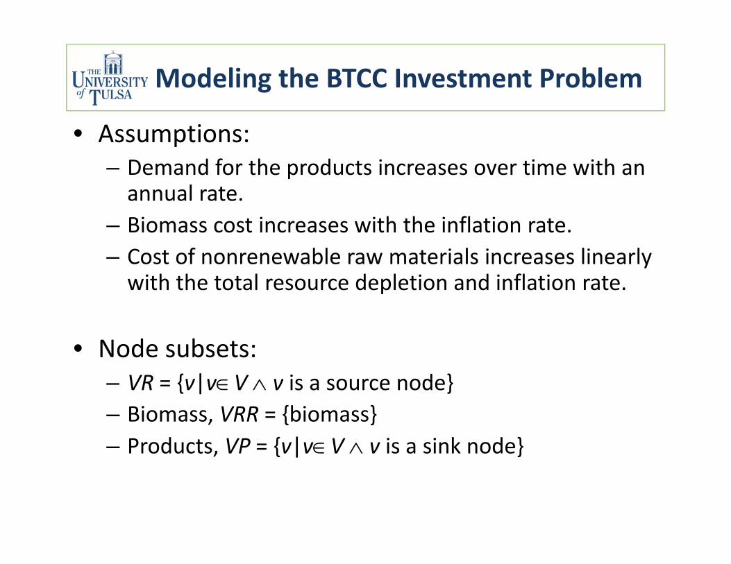
• Assumptions:– Demand for the products increases over time with an pannual rate.

– Biomass cost increases with the inflation rate.– Cost of nonrenewable raw materials increases linearly with the total resource depletion and inflation rate.

• Node subsets:– VR = {v|vV v is a source node}VR  {v|vV v is a source node}– Biomass, VRR = {biomass}– Products, VP = {v|vV v is a sink node}

Modeling the BTCC Investment Problem

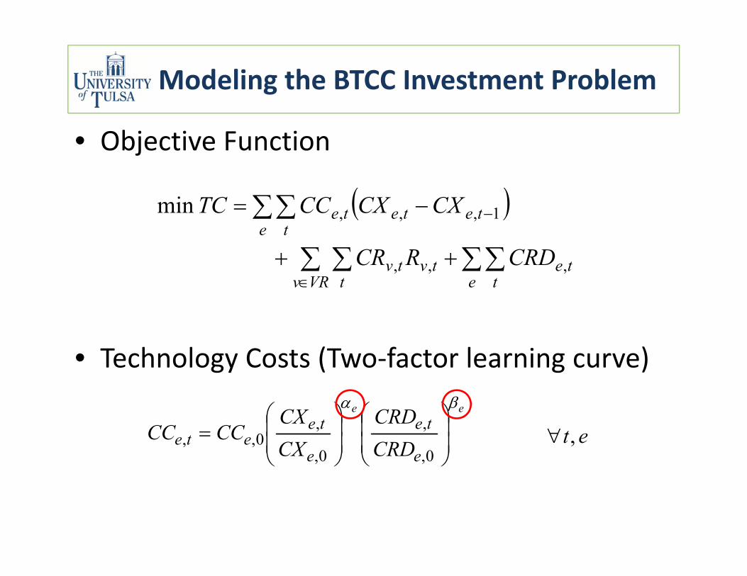
• Objective Function

e t

tetete

CRDRCR

CXCXCCTC 1,,, min

e t

teVRv t

tvtv CRDRCR ,,,

• Technology Costs (Two‐factor learning curve)ee

e

te

e

teete CRD

CRDCXCX

CCCC

0,

,

0,

,0,, et,

Modeling the BTCC Investment Problem

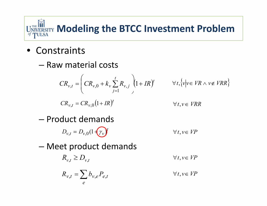
• ConstraintsRaw material costs– Raw material costs

tt

jjvvvtv IRRkCRCR

1

1,0,, VRRvVRvvt ,

d d d

j 1

tvtv IRCRCR 10,, VRRvt ,

– Product demandst

vvtv DD )1(0,, VPvt ,

– Meet product demandstvtv DR ,, VPvt ,

e

teevtv PbR ,,, VPvt ,

Modeling the BTCC Investment Problem

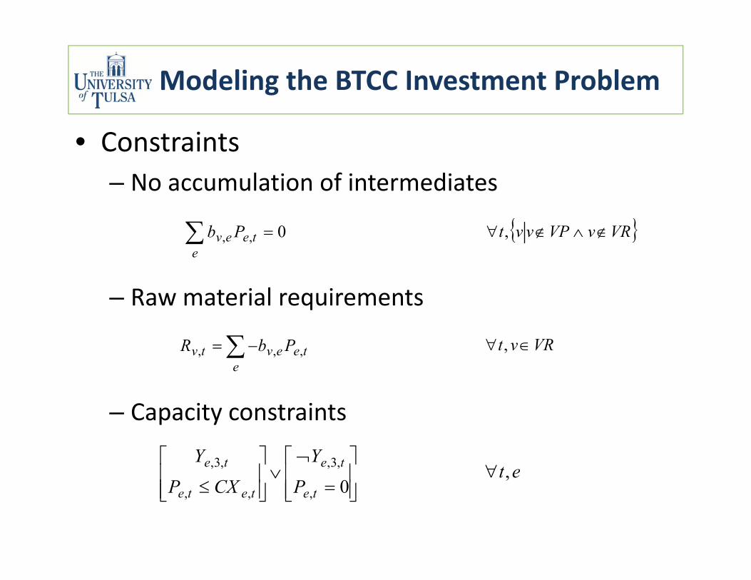
• ConstraintsNo accumulation of intermediates– No accumulation of intermediates

0,, e

teev Pb VRvVPvvt ,

– Raw material requirements

e

e

teevtv PbR ,,, VRvt ,

– Capacity constraints

,3,,3,

tete YY

et 0,,,

tetete PCXP

et,

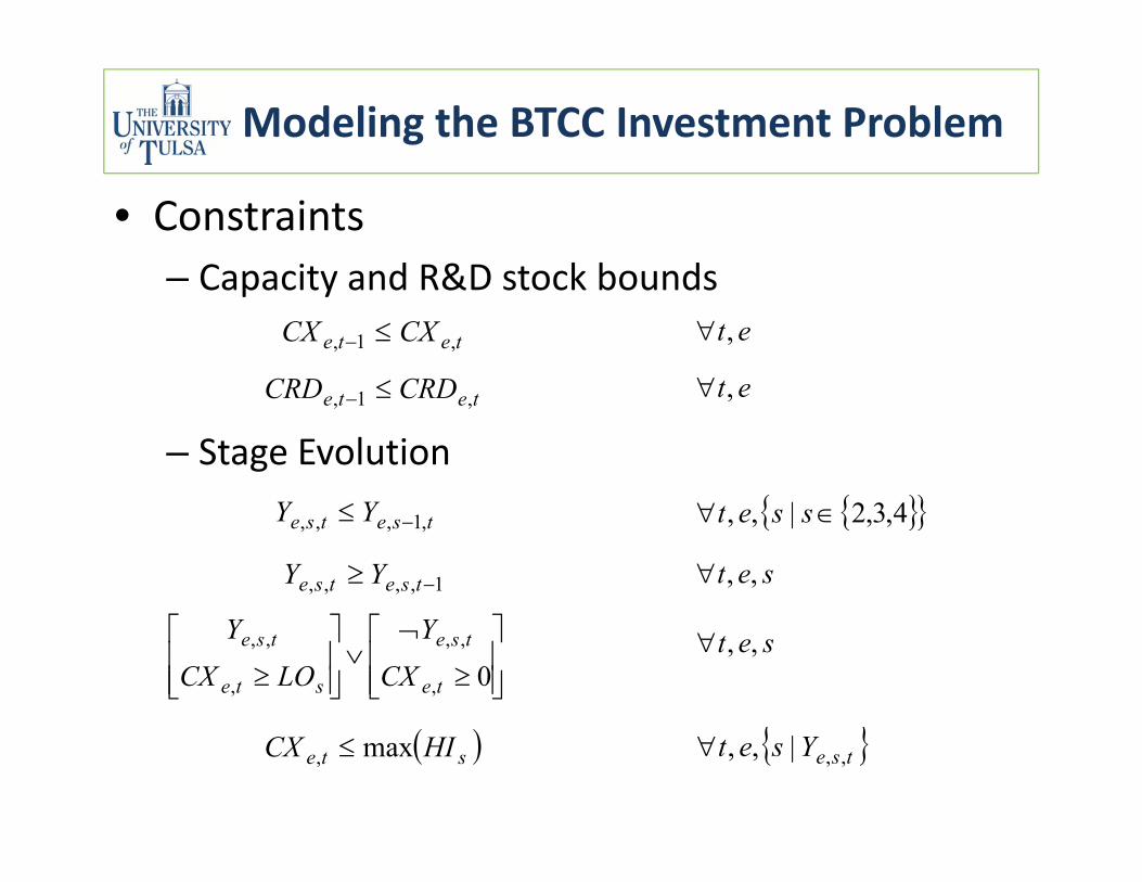
Modeling the BTCC Investment Problem

• ConstraintsCapacity and R&D stock bounds– Capacity and R&D stock bounds

tete CXCX ,1,

CRDCRD

et,

et

– Stage Evolutiontete CRDCRD ,1, et,

tsetse YY ,1,,, 4,3,2|,, sset

1,,,, tsetse YY set ,,

0,

,,

,

,,

te

tse

ste

tse

CXY

LOCXY set ,,

ste HICX max, tseYset ,,|,,

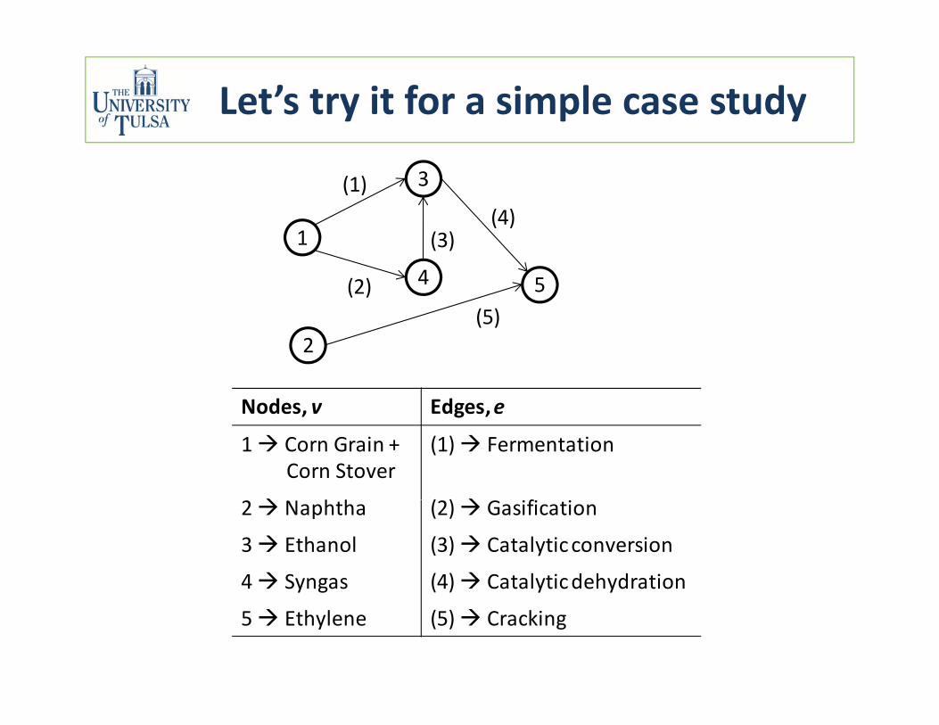
Let’s try it for a simple case study

3(1)(4)

1

4 5(2)

(3)( )

(5)2

(5)

Nodes v Edges eNodes, v Edges, e

1  Corn Grain +  Corn Stover

(1) Fermentation

h h ( ) f2  Naphtha (2)  Gasification

3  Ethanol (3)  Catalytic conversion

4  Syngas (4)  Catalytic dehydrationy g ( ) y y

5  Ethylene (5)  Cracking

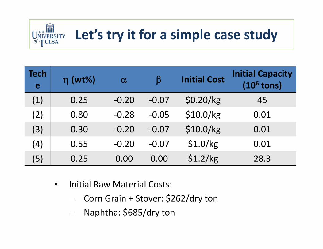
Let’s try it for a simple case study

Tech ( t%) I iti l C t Initial Capacity e (wt%) Initial Cost p y

(106 tons)(1) 0.25 ‐0.20 ‐0.07 $0.20/kg 45(2) 0.80 ‐0.28 ‐0.05 $10.0/kg 0.01(3) 0.30 ‐0.20 ‐0.07 $10.0/kg 0.01( ) $ /(4) 0.55 ‐0.20 ‐0.07 $1.0/kg 0.01(5) 0.25 0.00 0.00 $1.2/kg 28.3

• Initial Raw Material Costs:‒ Corn Grain + Stover: $262/dry tony‒ Naphtha: $685/dry ton

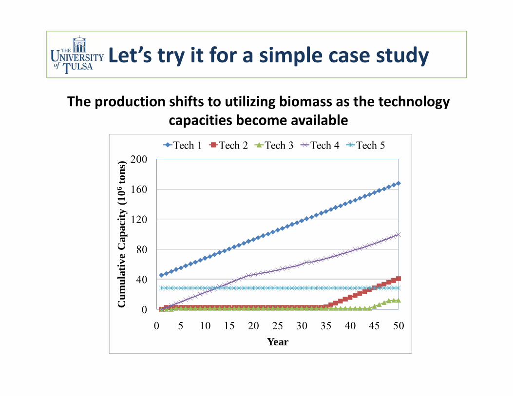
Let’s try it for a simple case study

The production shifts to utilizing biomass as the technology capacities become availablecapacities become available

200

ns)

Tech 1 Tech 2 Tech 3 Tech 4 Tech 5

120

160

city

(10

6to

n

80

ativ

e C

apac

0

40

0 5 10 15 20 25 30 35 40 45 50

Cum

ula

0 5 10 15 20 25 30 35 40 45 50Year

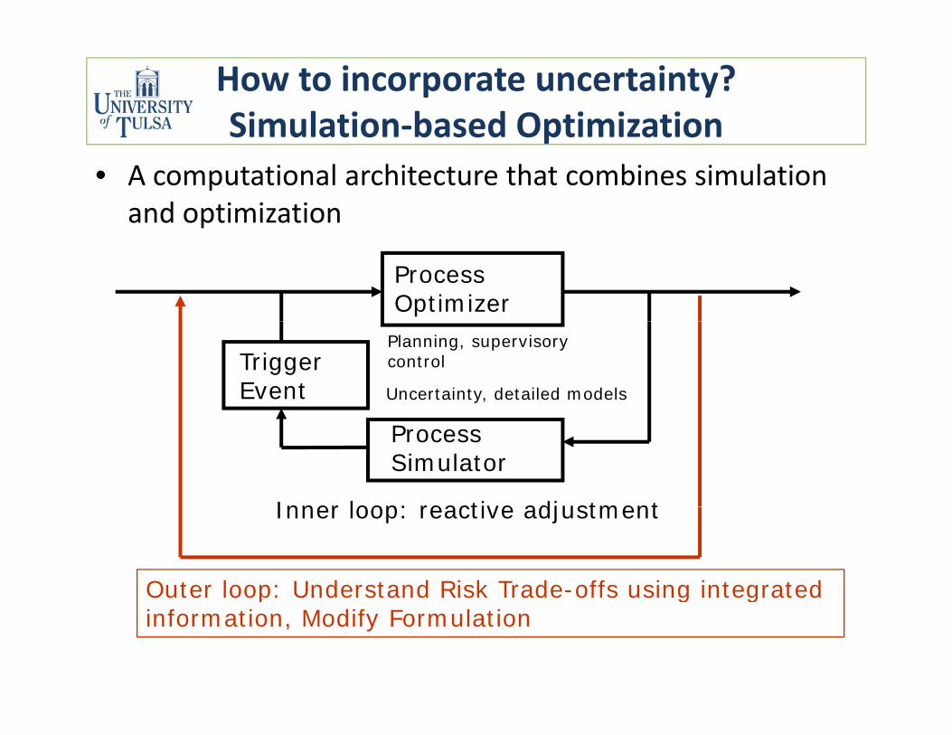
How to incorporate uncertainty? Simulation‐based OptimizationSimulation based Optimization

• A computational architecture that combines simulation and optimization

Process Optimizer

Trigger Event

Planning, supervisory control

Uncertainty, detailed models

Process Simulator

Inner loop: reactive adjustment

Outer loop: Understand Risk Trade-offs using integrated

Inner loop: reactive adjustment

p g ginformation, Modify Formulation

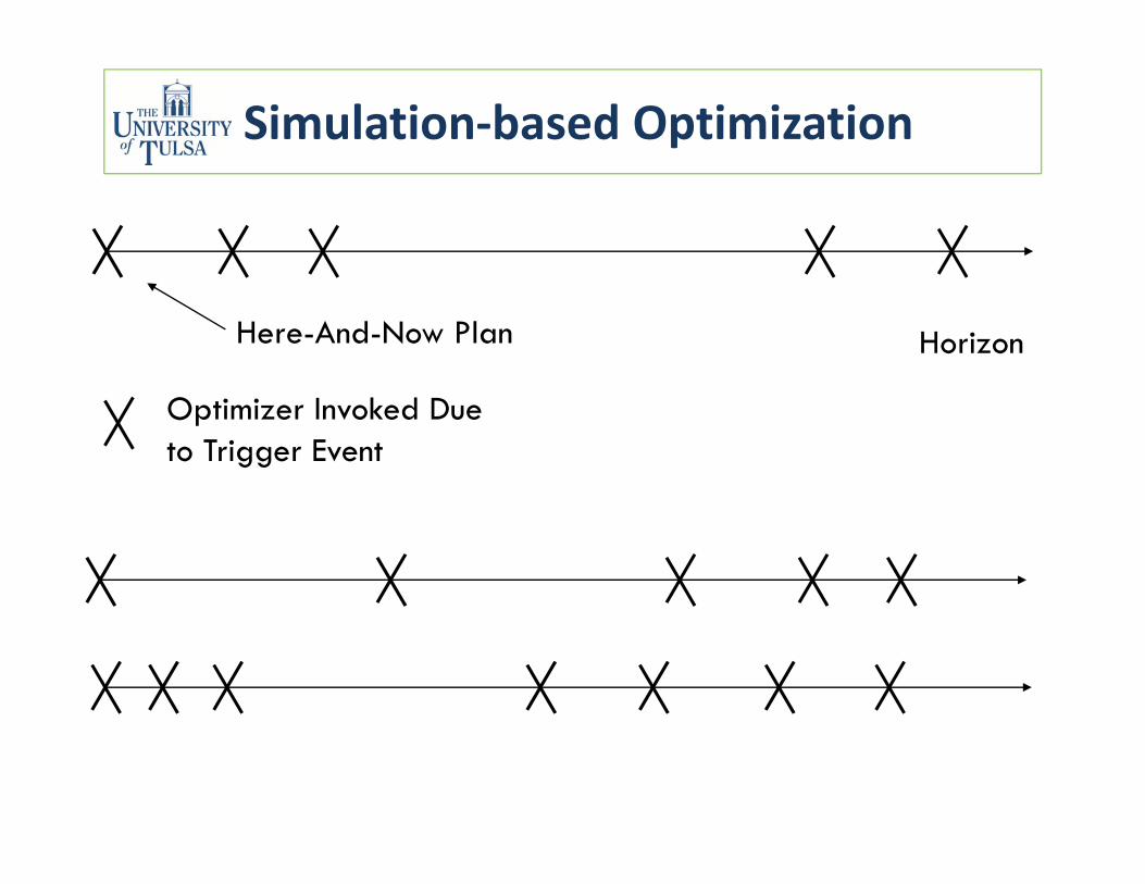
Simulation‐based Optimization

Here-And-Now Plan Horizon

Optimizer Invoked Due to Trigger Event

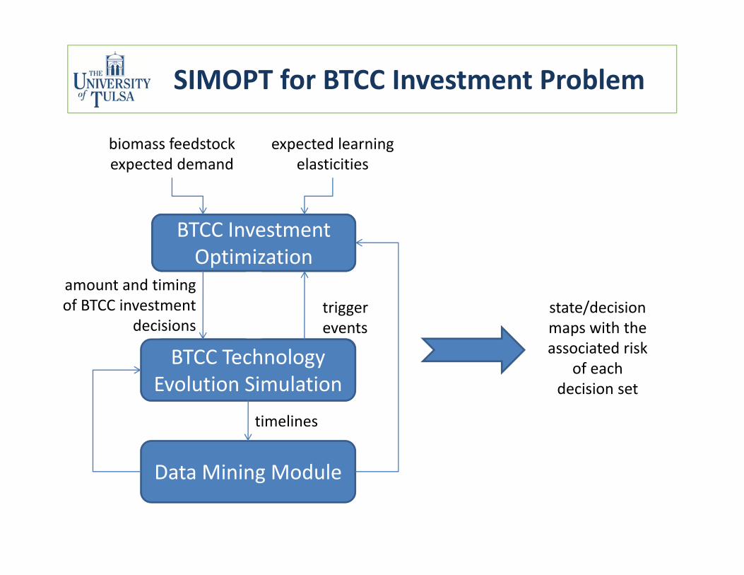
SIMOPT for BTCC Investment Problem

biomass feedstock expected demand

expected learning elasticities

BTCC Investment O ti i tiOptimization

amount and timing of BTCC investment 

decisionsstate/decision 

ith thtrigger 

t

BTCC Technology Evolution Simulation

decisions maps with the associated risk 

of each decision set

events

timelines

Data Mining ModuleData Mining Module

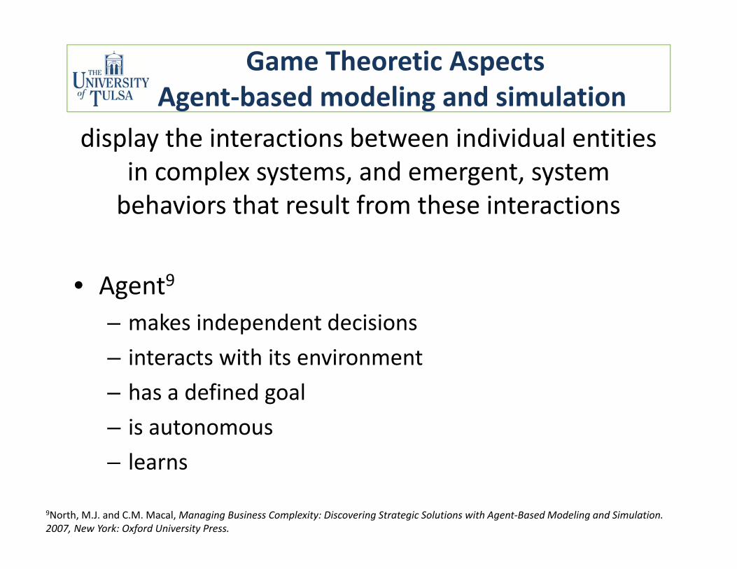
Game Theoretic AspectsAgent‐based modeling and simulationAgent based modeling and simulation

display the interactions between individual entities in complex systems and emergent systemin complex systems, and emergent, system behaviors that result from these interactions 

• Agent9

makes independent decisions– makes independent decisions– interacts with its environmenthas a defined goal– has a defined goal

– is autonomous– learnslearns

9North, M.J. and C.M. Macal, Managing Business Complexity: Discovering Strategic Solutions with Agent‐Based Modeling and Simulation. 2007, New York: Oxford University Press.

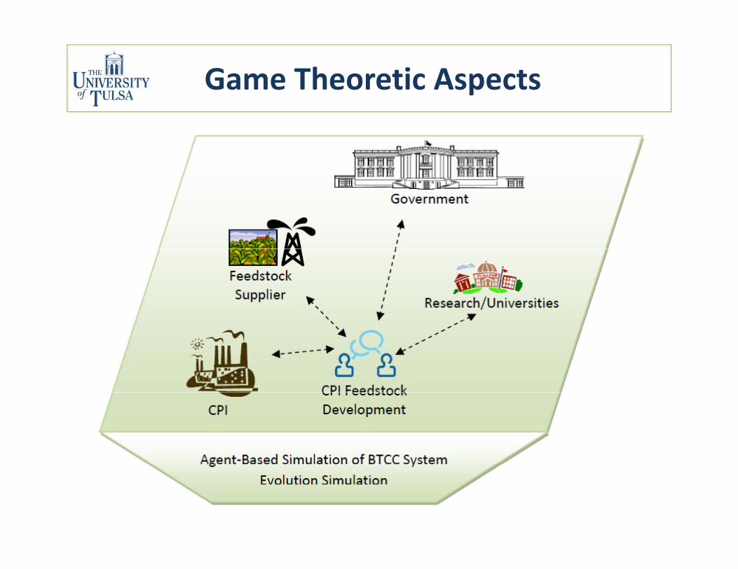
Game Theoretic Aspects

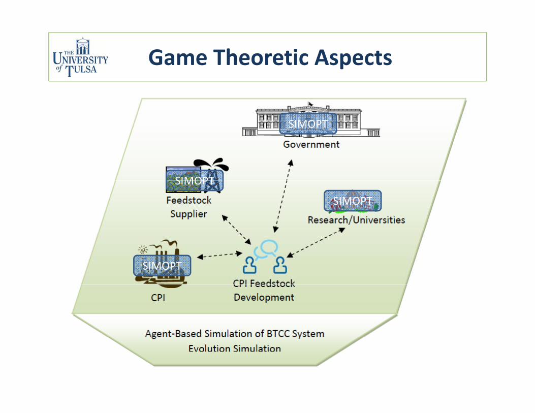
Game Theoretic Aspects

SIMOPT

SIMOPTSIMOPT

SIMOPT

SIMOPT

Acknowledgements

Graduate Students: Undergraduate Students:Ismail FahmiAroonsri NuchitprasittichaiByron Soepyan

gJohn EasonTyler Francis

y pySoumya YadalaJustin Smith

Financial support from NSF CAREER AwardFinancial support from NSF CAREER Award No 1055974 is greatly acknowledged.

Thank you

Questions?