HAL Id: hal-01195536https://hal.archives-ouvertes.fr/hal-01195536

Submitted on 7 Sep 2015

HAL is a multi-disciplinary open accessarchive for the deposit and dissemination of sci-entific research documents, whether they are pub-lished or not. The documents may come fromteaching and research institutions in France orabroad, or from public or private research centers.

L’archive ouverte pluridisciplinaire HAL, estdestinée au dépôt et à la diffusion de documentsscientifiques de niveau recherche, publiés ou non,émanant des établissements d’enseignement et derecherche français ou étrangers, des laboratoirespublics ou privés.

Model Predictive Control of a Direct Wave EnergyConverter Constrained by the Electrical Chain using an

Energetic ApproachThibaut Kovaltchouk, François Rongère, Muriel Primot, Judicael Aubry,

Hamid Ben Ahmed, Bernard Multon

To cite this version:Thibaut Kovaltchouk, François Rongère, Muriel Primot, Judicael Aubry, Hamid Ben Ahmed, et al..Model Predictive Control of a Direct Wave Energy Converter Constrained by the Electrical Chainusing an Energetic Approach. European Wave and Tidal Energy Conference 2015, Sep 2015, Nantes,France. �hal-01195536�

Model Predictive Control of a Direct Wave EnergyConverter Constrained by the Electrical Chain using

an Energetic ApproachThibaut Kovaltchouk∗†, Francois Rongere‡, Muriel Primot†,Judicael Aubry§, Hamid Ben Ahmed∗ and Bernard Multon∗

∗SATIE CNRS UMR8029, ENS Rennes, UEB, Avenue Robert Schuman, Bruz, France†IRCCyN, CNRS UMR6597, LUNAM, Ecole Centrale de Nantes, Nantes, France‡LHEEA, CNRS UMR6598, LUNAM, Ecole Centrale de Nantes, Nantes, France

§Mechatronics team, ESTACA, CERIE, Laval, France

Abstract—The control strategy for Direct Wave Energy Con-verters (DWEC) is often discussed without taking into accountthe physical limitations of electric Power Take-Off (PTO) system.This inappropriate modelling assumption leads to a non-realisticor a bad use of the electric systems, that leads to a failure tominimize the global ”per-kWh” system cost. We propose here aModel Predictive Control (MPC) that takes into account the mainlimits of an electrical chain: maximum force, maximum powerand a simplified loss model of the electrical chain. To compare thisoptimal control with other strategies, we introduce the notions ofcontrol, electric and global energy efficiencies. Furthermore, weuse an original energy representation used to value the state atthe end of the MPC horizon. Finally, we make several sensitivitystudy on the constraint limits for an economical pre-sizing of theelectrical chain.

Index Terms—Optimal Control, Model Predictive Control,Direct Wave Energy Converter, Pontryagin’s Maximum Principle,Direct Multiple Shooting Method, Energetic Model, ElectricPower Take-Off

NOMENCLATURE

A State matrix (6× 6) of the buoy systemArad State matrix (4× 4) of the radiation systema∞ Added mass of the buoy (radiation effect) [kg]b() Barrier functionBrad Input matrix (4× 1) of the radiation systemB1 Control matrix (6 × 1) of the buoy: system[

0 −(m+ a∞)−1 (0)]T

B2 Perturbation matrix (6×1) of the buoy system:[0 +(m+ a∞)−1 (0)

]TC Output matrix (1× 6) of the buoy system

c© 2015 European Wave and Tidal Energy Conference 2015. Personaluse of this material is permitted. Permission from European Wave and TidalEnergy Conference (EWTEC) must be obtained for all other uses, includingreprinting/republishing this material for advertising or promotional purposes,collecting new collected works for resale or redistribution to servers or lists,or reuse of any copyrighted component of this work in other works.Kovaltchouk, Thibaut; Rongere, Francois; Primot, Muriel; Aubry, Judicael;Ben Ahmed, Hamid; Multon, Bernard, ”Model Predictive Control of aDirect Wave Energy Converter Constrained by the Electrical Chain using anEnergetic Approach,” European Wave and Tidal Energy Conference, 2015,Nantes, pp.1,10, 6-11 September 2015ISSN 2309-1983, paper ID: 07D3-1

closs Electrical loss coefficient [W·N−2]closs Loss coefficient used in the control problem

[W·N−2]Crad Output matrix (1× 4) of the radiation systemEMech Mechanical energy stored in the system [J]f() Dynamic function of the buoy system x =

f(x, u, t)fexc Wave excitation force, time domain [N]Fexc Wave excitation force, Laplace domain [N]FMax Maximum Power Take-Off force [N]fPTO Power Take-Off force, time domain [N]FPTO Power Take-Off force, Laplace domain [N]H Hamiltonian of the control problem [W·kg−1]Hrad(s) Impulse radiation response, Laplace domain

[kg·s−1]Hs Significant height of the sea state [m]J Objective function of the control problem

[J·kg−1]khs Hydrostatic stiffness of the buoy [kg·s−2]L Lagrangian of the control problem [W·kg−1]m Mass of the buoy [kg]p Costate vector (1× 6)P Positive definite matrix: EMech = xT P xPLoss Mechanical power lost in the system [W]Pexc Excitation power fexcz [W]PMax Maximum Power Take-Off power [W]PPTO Power Take-Off mechanical power fPTO z [W]p2 Second element of pQ Positive definite matrix: PLoss = xT Q xTp Peak period of the sea state [s]u Control input of the buoy system: u = fPTO

w Perturbation input of the buoy system: w =fexc

x State vector (6 × 1) of the buoy system:[z z xrad

]Txrad State vector (4× 1) of the radiation systemx2 Second element of x: z

y Output of the buoy system: y = zz Vertical position of the buoy, time domain [m]Z Vertical position of the buoy, Laplace domain

[m]ε Parameter of the barrier function b()ηC Control energy efficiencyηE Electrical energy efficiencyψ() Weight of the final state [J·kg−1]

I. INTRODUCTION

Direct Wave Energy Converters (DWEC) (or Wave Acti-vated Bodies), with electric Power Take-Off (PTO) are oneof the most direct and flexible way to convert wave energyinto electrical energy, because there is no buffer between thewaves and the electrical chain contrary to Oscillating WaterColumn, Overtopping device or Wave Energy Converters withmechanical or hydropneumatic transmission. They may makeuse of mechanical transmission (gear box, rack and pinion, etc)or may not (direct drive). They lead to the possibility of higherefficiency and reliability, yet feature higher power fluctuationsin the grid than WEC with hydraulic or mechanical storagesystems. The test case considered here to represent DWECs isa heaving buoy, but the method can be reused for all DWECwith electric PTO.

In order to minimize the per-kWh cost of this technology,the global efficiency from wave to wire must increase, whilelimiting the size of the electric PTO (classically an electricalmachine with an active rectifier).

Control design, however, must take into account the mainlimitations of an electric PTO, i.e.: power limitation, forceor torque limitation and losses in the electric chain. But theproblem is often seen as decoupled. Thus, two types of papersclassically deal with control strategies in DWEC: the theoreti-cal optimization of control with no or very little considerationsfor the feasibility limitations [1]–[3]; and optimization using agiven electric system [4]. Some studies take into account onlylosses [5], [6], or power limitation [7], or force limitation [8].To the best of our knowledge, it is the first time a ModelPredictive Control of a Wave Energy Converter takes intoaccount all the main constraints of an electrical chain.

Furthermore, only a few papers have dealt with the couplingbetween control strategy and sizing [9].

II. MODELS

A. Dynamic Model of the Buoy

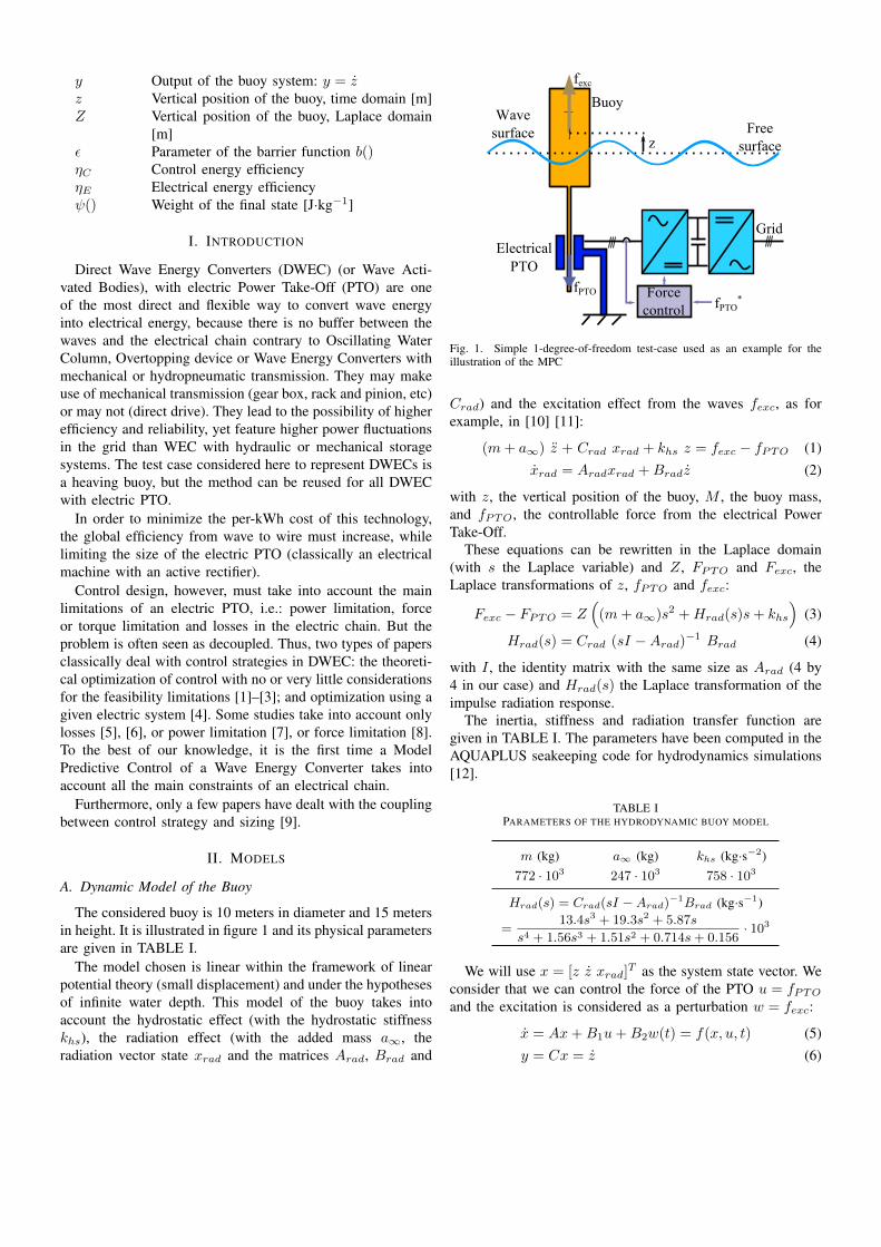
The considered buoy is 10 meters in diameter and 15 metersin height. It is illustrated in figure 1 and its physical parametersare given in TABLE I.

The model chosen is linear within the framework of linearpotential theory (small displacement) and under the hypothesesof infinite water depth. This model of the buoy takes intoaccount the hydrostatic effect (with the hydrostatic stiffnesskhs), the radiation effect (with the added mass a∞, theradiation vector state xrad and the matrices Arad, Brad and

Buoy

Electrical PTO

z

fexc

fPTO

Free surface

Wave surface

Forcecontrol fPTO

*

Grid

Fig. 1. Simple 1-degree-of-freedom test-case used as an example for theillustration of the MPC

Crad) and the excitation effect from the waves fexc, as forexample, in [10] [11]:

(m+ a∞) z + Crad xrad + khs z = fexc − fPTO (1)xrad = Aradxrad +Bradz (2)

with z, the vertical position of the buoy, M , the buoy mass,and fPTO, the controllable force from the electrical PowerTake-Off.

These equations can be rewritten in the Laplace domain(with s the Laplace variable) and Z, FPTO and Fexc, theLaplace transformations of z, fPTO and fexc:

Fexc − FPTO = Z(

(m+ a∞)s2 +Hrad(s)s+ khs

)(3)

Hrad(s) = Crad (sI −Arad)−1 Brad (4)

with I , the identity matrix with the same size as Arad (4 by4 in our case) and Hrad(s) the Laplace transformation of theimpulse radiation response.

The inertia, stiffness and radiation transfer function aregiven in TABLE I. The parameters have been computed in theAQUAPLUS seakeeping code for hydrodynamics simulations[12].

TABLE IPARAMETERS OF THE HYDRODYNAMIC BUOY MODEL

m (kg) a∞ (kg) khs (kg·s−2)772 · 103 247 · 103 758 · 103

Hrad(s) = Crad(sI −Arad)−1Brad (kg·s−1)

=13.4s3 + 19.3s2 + 5.87s

s4 + 1.56s3 + 1.51s2 + 0.714s+ 0.156· 103

We will use x = [z z xrad]T as the system state vector. Weconsider that we can control the force of the PTO u = fPTO

and the excitation is considered as a perturbation w = fexc:

x = Ax+B1u+B2w(t) = f(x, u, t) (5)y = Cx = z (6)

with A, B1, B2 and C, respectively the state, the control,the perturbation and the output matrices of the buoy systemthat takes as inputs forces (u and w) and that gives the speedof the buoy as an output (y). The speed was chosen as theonly output because this variable is linked with the excitationpower Pexc = z fexc and the PTO mechanical power PPTO =z fPTO. It has been verified that this system is controllableand observable.

A JONSWAP spectrum is used to compute the excitationforce [13]. The frequency spreading parameter γ was chosenequal to 3. The excitation force time series (correspondingto wave data) is generated by summing monochromatic exci-tation with randomly chosen initial phases. In our case, thisconfiguration is similar to the solution of a reconstructed waveelevation with a random phase, as presented in [14].

This dynamic equation is solved using the Heun’s ordinarydifferential equation solver (explicit trapezoidal rule) with afixed time step of 0.1 s.

B. Energetic Model of the Buoy

Because the model is linear and passive, there exist a coupleof two positive semidefinite matrices P and Q that defines themechanical energy stored in the system and the power losswith the radiation effects:

EMech = xT P x (7)PLoss = xT Q x (8)

These two terms respect the conservation of energy with thefollowing equation:

EMech = Pexc − PPTO − PLoss (9)

with the excitation power Pexc and the PTO mechanical powerPPTO.

In order to find these two equations, we need to solvethe following semidefinite programming problem, for examplewith CVX [15]:

BT2 (2 P ) = C (10)

AT P + P A+Q = 0 (11)

Fig. 2 illustrates a decay test used to test the accuracy of thisenergetic model: without excitation and harvesting, the timederivative of the mechanical energy corresponds exactly to themechanical loss xT Q x. Such a model gives information onpower flows that is essential for energy conversion studies.

C. Model of the Electrical Chain

The electrical chain is simplified by considering two con-straints and one term of losses.

The absolute value of the force is limited by a maximumvalue FMax mainly due to the limitation of the electricalmachine (electromagnetic converter) and the absolute valueof the power is limited by a maximum value PMax due to thelimitation of the active rectifier (power electronics converter).

Finally, we subtract from the mechanical power of the PTOsystem, electric losses assumed to be proportional to the square

0 50 100 150 200

−2

0

2

z (

m)

0 50 100 150 200

−2

0

2

v (

m/s

)

0 50 100 150 2000

0.5

1

EM

ech (

kW

h)

0 50 100 150 2000

50

100

Time (s)

PLo

ss (

kW

)

d ESto

/ dt

xT Q x

Fig. 2. Decay test from a height of 3 meters: position, speed, energy andpower loss vs. time

value of the force. More precise model could take into accountcopper and iron losses in the electrical machine as well asconduction and switching losses in the active rectifier [9].

This model can be summarized by figure 3 or these threeequations:

|fPTO| ≤ Fmax (12)|fPTO · z| ≤ Pmax (13)

PGrid = fPTO · z − closs f2PTO (14)

Velocity (m/s)

Forc

e (

MN

)

Electrical power

−4 −2 0 2 4

−1

−0.5

0

0.5

1

Pele

c (

MW

)

−1

−0.5

0

0.5

1

Velocity (m/s)

Losses

−4 −2 0 2 4

−1

−0.5

0

0.5

1

Plo

ss (

kW

)

0

25

50

75

100

Fig. 3. Electrical power and electrical loss power as a function of Buoy veloc-ity z and Power Take-Off force fPTO with Fmax =1 MN, Pmax =1 MWand closs =0.1 MW/MN2

D. Energy Efficiency

Control efficiency is defined with the maximal theoreticalrecoverable power PWave as in [11]. With the wave spectrumused in our case, we have:

PWave ≈ 103 H2s T

3p (15)

with Hs and Tp, respectively the significant height and thepeak period of the sea state considered.

So we define the energy efficiency of the control ηC and ofthe electrical chain ηE as:

ηC =PPTO

PWave

(16)

ηE =PGrid

PPTO

(17)

ηC ηE =PGrid

PWave

(18)

III. MODEL PREDICTIVE CONTROL WITH PONTRYAGIN’SMAXIMUM PRINCIPLE

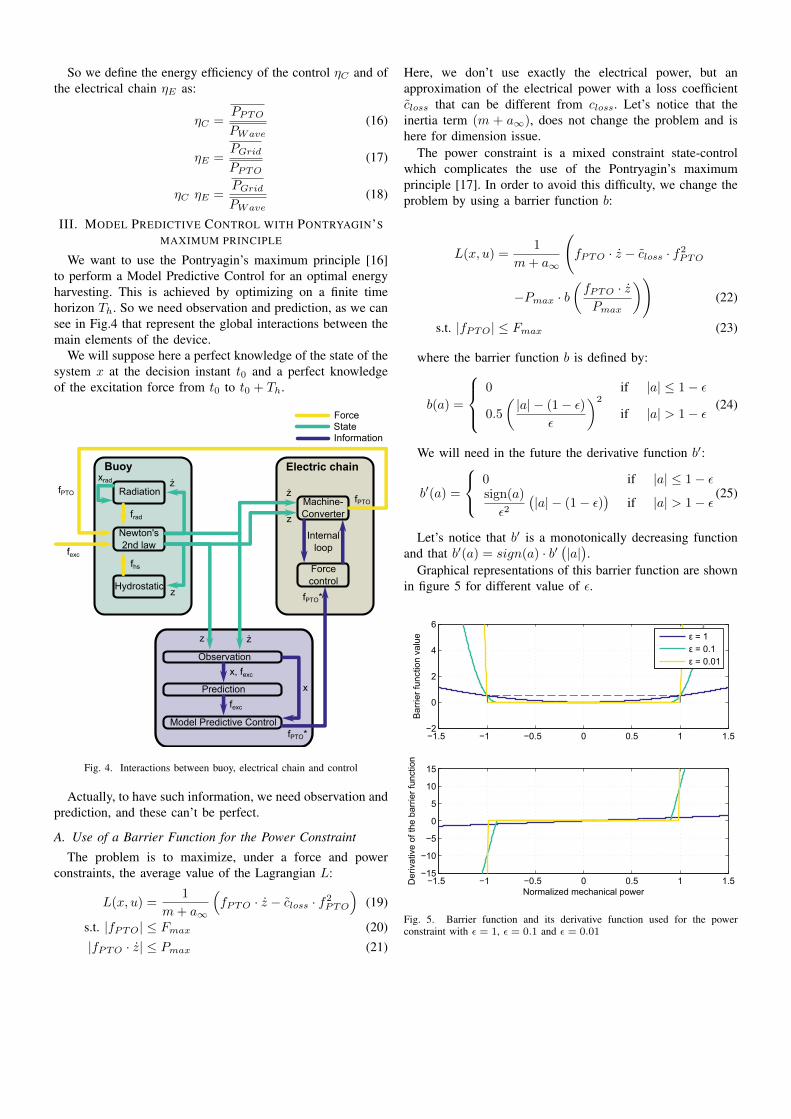
We want to use the Pontryagin’s maximum principle [16]to perform a Model Predictive Control for an optimal energyharvesting. This is achieved by optimizing on a finite timehorizon Th. So we need observation and prediction, as we cansee in Fig.4 that represent the global interactions between themain elements of the device.

We will suppose here a perfect knowledge of the state of thesystem x at the decision instant t0 and a perfect knowledgeof the excitation force from t0 to t0 + Th.

Buoy Electric chain

Observation

Prediction

ModelTPredictiveTControl

Hydrostatic

Radiation

Newton.s2ndTlaw

ForceStateInformation

z

fPTO

fexc

frad

fhs

fPTO

x,Tfexc

x

fexc

fPTO*z

Forcecontrol

Machine-Converter

InternalTloop

z

fPTO*

xrad .z .

z

.z

Fig. 4. Interactions between buoy, electrical chain and control

Actually, to have such information, we need observation andprediction, and these can’t be perfect.

A. Use of a Barrier Function for the Power Constraint

The problem is to maximize, under a force and powerconstraints, the average value of the Lagrangian L:

L(x, u) =1

m+ a∞

(fPTO · z − closs · f2PTO

)(19)

s.t. |fPTO| ≤ Fmax (20)|fPTO · z| ≤ Pmax (21)

Here, we don’t use exactly the electrical power, but anapproximation of the electrical power with a loss coefficientcloss that can be different from closs. Let’s notice that theinertia term (m + a∞), does not change the problem and ishere for dimension issue.

The power constraint is a mixed constraint state-controlwhich complicates the use of the Pontryagin’s maximumprinciple [17]. In order to avoid this difficulty, we change theproblem by using a barrier function b:

L(x, u) =1

m+ a∞

(fPTO · z − closs · f2PTO

−Pmax · b(fPTO · zPmax

))(22)

s.t. |fPTO| ≤ Fmax (23)

where the barrier function b is defined by:

b(a) =

0 if |a| ≤ 1− ε

0.5

(|a| − (1− ε)

ε

)2

if |a| > 1− ε(24)

We will need in the future the derivative function b′:

b′(a) =

0 if |a| ≤ 1− εsign(a)

ε2(|a| − (1− ε)

)if |a| > 1− ε

(25)

Let’s notice that b′ is a monotonically decreasing functionand that b′(a) = sign(a) · b′

(|a|).

Graphical representations of this barrier function are shownin figure 5 for different value of ε.

−1.5 −1 −0.5 0 0.5 1 1.5−2

0

2

4

6

Bar

rier

func

tion

valu

e

−1.5 −1 −0.5 0 0.5 1 1.5−15

−10

−5

0

5

10

15

Normalized mechanical power

Der

ivat

ive

of th

e ba

rrie

r fu

nctio

n

ε = 1ε = 0.1ε = 0.01

Fig. 5. Barrier function and its derivative function used for the powerconstraint with ε = 1, ε = 0.1 and ε = 0.01

B. Objective FunctionThe objective function to maximize is J defined at each

time t0 by:

J(t0) =

∫ t0+Th

t0

L(x, u) dt+ Ψ(x(t0 + Th)) (26)

The function Ψ gives a weight to the final horizon state.Without such weight, the control naturally tends to convert allthe energy stored by the DWEC at the end of the horizon. Wewill here use a portion α of the mechanical energy EMech

that can be used after the horizon:

Ψ(x) =1

m+ a∞· α · EMech(x) (27)

=1

m+ a∞· α · xT P x (28)

With α = 0, we consider that this energy has no value, andwith α = 1, we consider that this energy has the same valueas the energy converted during the time horizon.

C. Hamiltonian and Dynamic of the Costate vectorThe Hamiltonian is defined by:

H = pT f(x, u, t) + L(x, u) (29)

with p, the costate vector, of the same size as the state vector.The dynamic of this costate vector p is:

p = −∂H∂x

(30)

= −AT p+B1 fPTO

[1− b′

(z · fPTO

PMax

)](31)

And the final costate value must satisfy the followingtransversal condition:

p(t0 + Th) =∂Ψ

∂x(32)

=1

m+ a∞· α · 2 P x(t0 + Th) (33)

D. Maximization of the HamiltonianThe Pontryagin’s maximum principle states that the maxi-

mization of the function J is obtained only if the control fPTO

maximizes the Hamiltonian H at all instant t.There are two possibilities:• The maximum of the Hamiltonian is in the admissible

control interval (|fPTO| ≤ Fmax);• The maximum of the Hamiltonian is outside the admis-

sible control interval: fPTO = sign(

∂H∂fPTO

)Fmax.

We begin by making the hypothesis that we are in the firstcase. To find the extremum of the Hamiltonian, we calculateits derivative function:

∂H

∂fPTO

=1

m+ a∞

−p2 + z

[1− b′

(z · fPTO

Pmax

)]

−2 · closs · fPTO

(34)

With the information given by the derivative of the barrierfunction, we can rewrite this expression:

∂H

∂fPTO

=1

m+ a∞

(−p2 + z − |z|b′

(|z| · fPTO

Pmax

)

−2 · closs · fPTO

)(35)

This function is strictly decreasing with respect to fPTO, sothere is only one global extremum, and it is always a maximumbecause the derivative function changes sign from positive tonegative:

0 = −p2 + z − |z|b′(|z| · fPTO

Pmax

)− 2 · closs · fPTO (36)

In this case, the sign of fPTO is always the same as thesign of (z − p2) because the function is strictly decreasingand y-intercept equals (z − p2) (see Fig. 6).

+ Fmax

- Fmax

∂H∂fPTO

fPTO

Max(H)

Fig. 6. Maximization of the Hamiltonian performed by the study of itsderivative. Eight different cases are illustrated here according to the sign of(z − p2), the influence of the barrier function for the passage by zero and ifthe passage by zero is in or out the admissible domain.

Three different cases exist, that depend on the mechanicalpower fPTO · z:• |fPTO · z| ≤ (1− ε) · Pmax;• fPTO · z > (1− ε) · Pmax;• fPTO · z < −(1− ε) · Pmax;And the respective solutions are:

• fPTO =z − p22 · closs

;

• fPTO =(z − p2) · ε2 + z · (1− ε)2 · closs · Pmax · ε2 + z2

Pmax ≈Pmax

z;

• fPTO =(z − p2) · ε2 − z · (1− ε)2 · closs · Pmax · ε2 + z2

Pmax ≈ −Pmax

z;

Let’s notice that the value of the parameter ε has no effectbecause of the simplification done in these solutions.

So, we consider the first case. If the result does not respectthe condition, we use the second or the third case accordingto the sign of (z − p2).

If the force fPTO respects the force constraint, the problemis solved; if not, we know that the force constraint must bemet. To maximize the Hamiltonian, we must use the followingrelation:

fPTO = sign

(∂H

∂fPTO

)Fmax (37)

We have already seen that the derivative of the Hamiltonianhas only one sign change, and it is outside the control intervalin this case. So the sign of the derivative in the control intervalis the same (see Fig. 6), and in particular:

sign

(∂H

∂fPTO

)= sign

(∂H

∂fPTO(fPTO = 0)

)(38)

= sign (z − p2) (39)

So, we finally have:

fPTO = sign (z − p2)Fmax (40)

The complete algorithm to find the optimal fPTO as afunction of the state vector x and the costate vector p isillustrated in Fig. 7.

fPTO = 2 closs

x2 - p2

|fPTO x2| > Pmax

b' = 0Pmax

fPTO x2( )

fPTO = Pmax

|x2|

=x2

2 closs fPTO - (x2 - p2)b'Pmax

fPTO x2( )

|fPTO| > Fmax

b' = 0Pmax

fPTO x2( )fPTO = Fmax sgn(x2 -p2)

Begin

End

sgn(x2 -p2)

Fig. 7. Algorithm used to maximize the Hamiltonian as a function of thestate vector x and the costate vector p.

E. MPC resolution

A standard multiple shooting method [18] was used to solvethis MPC problem. We can sum up the dynamic and the controlrelations with these three equations:

x =∂H

∂p(t, x, p, u) (41)

p = −∂H∂x

(t, x, p, u) (42)

u = fPTO(x, p) (43)

If we rewrite these relations with z =[x p

]T, we can

have:

z =

∂H

∂p(t, z, fPTO(z))

−∂H∂x

(t, z, fPTO(z))

= F (t, z) (44)

With the simple shooting method, we want to find zsol(t0)in such a way that the two boundaries conditions are met:

xsol(t0) = x(t0) (45)

psol(t0 + Th) =1

m+ a∞· α · 2 P x(t0 + Th) (46)

Compared to the simple method of shooting, multiple shoot-ing method consists of cutting the interval into N intervals, andsearching the z values at the beginning of each sub-interval.We must take into account matching conditions between thesub-intervals.

We improve the stability of the method by increasing thenumber of nodes, but the problem becomes bigger. Indeed,each new node adds 12 new variables that need to be found (6for the state and 6 for the costate). This is indeed the principleof the multiple shooting method, as opposed to the simpleshooting method where the errors with respect to the initialcondition increase exponentially with the horizon size Th.

With the multiple shooting method, we want to find, forexample, zsol1(t0) and zsol2(t0 + Th/2) such as:

xsol1(t0) = x(t0) (47)zsol1(t0 + Th/2) = zsol2(t0 + Th/2) (48)

psol2(t0 + Th) =1

m+ a∞· α · 2 P x(t0 + Th) (49)

The problem has been subdivided by two in this example butit can be subdivided by more than two.

To solve this problem, we use the Maltab function fsolve().

IV. RESULTS

The MPC control described in III has been simulated withthe buoy model. Each 0.5 s, the optimal control is used tocompute the costate vector in order to decide the next PTOforce to be applied in the next 0.5 s. We have consideredthis time to be short enough for the control performances,but the sampling time used in the MPC algorithm is still0.1 s. It seems that it is possible to obtain real-time computingwith numerical optimization and the use of correct technology(like Digital Signal Processors or Field-Programmable GateArrays). Indeed, it takes around 0.5 s for reasonable timehorizon to compute the control with an Intel-Xeon X5550clocked at 2.67 GHz. Table II gives the default parameters

used in this study: if no further information is given, theseparameters are used. Each simulation has a duration of 250 sin order to model one sea state.

TABLE IIMODEL PREDICTIVE CONTROL DEFAULT PARAMETERS

Maximum PTO force Fmax 1 MN

Maximum PTO power Pmax 1 MW

Loss coefficient closs 0.1 MW/MN2

Control loss coefficient closs 0.1 MW/MN2

Time horizon Th 12 s

Weight of the final state energy α 0.5

Fig. 8 illustrates for one sea state (Hs = 2 m, Tp = 8 s)two different types of control: an optimized passive controlwith the PTO force proportional to the speed and the MPCresults. We can verify that the force and the power constraintsare respected, while the PTO force is much more continuousthan typical bang-bang controls [19]. The average productionfor the passive control is 45 kW and 110 kW for the MPC, thatis around two times more.

0 50 100 150−5

0

5MPC

0 50 100 150−5

0

5

0 50 100 150

−1000

0

1000

0 50 100 150

−1000

0

1000

Time (s)

0 50 100 150−5

0

5

z (

m)

Passive

0 50 100 150−5

0

5

v (

m/s

)

0 50 100 150

−1000

0

1000

f PT

O (

kN

)

0 50 100 150

−1000

0

1000

Pele

c (

kW

)

Time (s)

Fig. 8. Comparison between an optimized passive control and the ModelPredictive Control (sea state: Hs = 2m, Tp = 8 s with the same excitationprofile)

A. Influence of the time horizon and the weight of the finalmechanical energy

Two parameters have a huge influence on the controlperformance: the time horizon Th and the weight of final statemechanical energy α. We can predict that the performance isglobally increasing with the time horizon, because we use aperfect prediction of the excitation. This is what we observein figure 9.

The influence of the coefficient α must be lower for a biggerhorizon Th, because this energy become smaller compared tothe converted energy. We can also observe this in figure 9.

0 10 20−50

−25

0

25

50

Horizon Th (s)

Glo

bal effic

iency η

C η

E (

%)

α = 0 %

α = 50 %

α = 80 %

α = 100 %

0 50 100−50

−25

0

25

50

Final energy considered α (%)

Th = 1 s

Th = 3 s

Th = 10 s

Th = 20 s

Fig. 9. Control performance for different time horizon Th and weight of finalstate mechanical energy α (sea state: Hs = 3m, Tp = 9 s with the sameexcitation)

We can deduce from figure 9 that, for each time horizon Th,there exists an optimal value of α between 0 and 100 % thatmaximize the performance of the control, that is the electricalenergy converted. This optimum is smaller with larger timehorizon and its limit seems to be 0.

Others MPC controls for wave energy converters do not takeinto account the final state energy (that correspond to the caseα = 0): we can see an important benefit with this additionalsetting parameter, in particular with small time horizon value.That could be very important if the numerical complexity orthe prediction quality does not allow to have long time horizon.

But we see also that taking into account all the final stateenergy (α = 1) is never the best way to maximize theperformance, because this mechanical energy have less valuethan converted energy: we can even see that, for small timehorizon, the wave energy converter consumes more energythan it produces.

B. Influence of the sea state

The performance of the control is different for each seastate, depending on how far the peak period of the excitation isfrom the natural resonant period of the system without control(here, around 7.2 s) and how powerful the sea state is (becausea calm sea state needs less PTO force to have a good controlefficiency). We can notice in figure 10 that the global efficiencyis higher for relatively calm sea state and a peak period closeto the natural resonant period.

We can notice that the shape of the global efficiency as afunction of the time horizon is similar for all sea states, butit would no longer be the case with a real prediction of theexcitation force.

C. Influence of an error and the electrical losses model

Apart from taking into account the final state energy inthe MPC control, a second originality is to take into accounta simplified loss model for the electrical chain. So it is

0 5 10 15 200

20

40

60

80

Time−horizon Th (s)

Glo

ba

l e

ffic

ien

cy η

C η

E (

%)

7 s, 2 m

11 s, 1 m

8 s, 2 m

9 s, 3 m

11 s, 5 m

Fig. 10. Harvesting performance versus time horizon Th for different seastates

important to evaluate what has been added with this additionalinformation by a sensitivity study, illustrated by the figure11: the hypothesis about the electrical chain is the same(closs = 0.1 MW/MN2) but we change the coefficient use forthe control (closs from 0.01 to 1 MW/MN2).

10−1

100

101

25

50

75

100

Effi

cien

cy˜(

%)

Error˜factor˜on˜the˜control˜loss˜coefficient˜closs

/closs

Powerful˜sea−state˜(9˜s,˜3˜m)

˜

˜

10−1

100

101

25

50

75

100

Effi

cien

cy˜(

%)

Calm˜sea−state˜(7˜s,˜2˜m)

˜

Control˜ηC

Electrical˜ηE

Global˜ηCη

E

Fig. 11. Control efficiency, electrical efficiency and global efficiency withthe same hypothesis but an error on the loss coefficient

We can predict that the control efficiency will be higher andthe electric efficiency will be smaller for a smaller value ofcloss. The maximum value of the global efficiency must cor-respond to closs = closs = 0.1 MW/MN2. This corresponds tothe results show in figure 11. We can notice that an importanterror on the loss model (by a factor 10) has perceptible impacton global efficiency, but it is not the case for a smaller error(by a factor 3), that could still be considered as an importanterror. Our MPC seems quite robust against a modelling errorin the loss coefficient.

We can notice that it is more important to take into accountlosses for calm sea state, because the control efficiency forpowerful sea states is already limited by the maximum forceand the maximum power for powerful sea states.

D. Pre-sizing of the electrical chain

One important decision to be made for the design of a WaveEnergy Converter is the size of its Power Take-Off. Here weinvestigate the influence of maximum force and maximumpower on the global efficiency of the conversion, but also onthe total profitability (that is the reduction of the per-kWhcost). Indeed, a bigger Power take-Off allows directly a moreefficient conversion, but with a bigger cost, that is not alwaysthe best way for the global per-kWh cost.

The total energy produced during the lifetime of a DirectWave Energy Converter EProd correspond to a 8 years casewith the sea state (9 s, 3 m), hypothetically equivalent to20 years in Yeu’s island site [20]. We can see the increaseof EProd with the maximum force and the maximum powerin the first subfigure (Buoy profitability) of figure 12.

The second and the third subfigures of figure 12 (static andelectro-mechanical converter profitability) correspond respec-tively to the ratio between the energy produced during itslifetime by the WEC EProd and the maximum power (forthe static converter profitability) or the maximum force (forthe electro-mechanical converter profitability). Indeed, we usethe assumption that the maximum power depends mainly onthe static converter size and the maximum force on the electro-mechanical converter (machine) size.

We deduce a cost per-kWh CkWh with the followinghypotheses:• Static converter cost CP : 100 ke/MW ;• Electro-mechanical converter cost CF : 200 ke/MN ;• Cost of the installed DWEC without the electrical chainCB : 2000 ke.

So we can calculated CkWh with the following relation:

CkWh =CB + CP PMax + CF FMax

EProd(50)

The last figure (Total profitability) correspond to the inverseof this value. We can cite the French WEC feed-in tariff forcomparison, that corresponds to 6.7 kWh/e. According to thisstudy, an electrical chain with a 2 MW converter and a 2 MNelectrical machine has a smaller per-kWh cost than smallerelectrical chain.

V. CONCLUSION

This paper proposes an enhanced Model Predictive Controlfor a Wave Energy Converter (in this case, a heaving buoy):this model takes into account an original energetic model andthe main constraints of an electrical chain (limitation in force,in power and losses depending on Power Take-Off force).

The mixed constraint on the power is taken into accountwith a barrier function, in order to use the maximum Pontrya-gin’s principle. A classical multishooting method is used tocompute the optimal control.

The results of the control are consistent with most intuitions.The control is close of its maximum performance from 12 stime horizon (the natural resonant period of the system is7.2 s). Considering final state energy in the control allowsbetter performance for shorter time horizon, that could be

Max. Force FMax

(MN)

Ma

x.

po

we

r P

Ma

x (

MW

)

Buoy profitability

0.25 1 40.25

1

4

EP

rod

. (GW

h)

0

12

24

Max. Force FMax

(MN)

Ma

x.

po

we

r P

Ma

x (

MW

)

Static converter profitability

0.25 1 40.25

1

4

EP

rod

. /PM

ax (G

Wh

/MW

)

0

20

40

Max. Force FMax

(MN)

Ma

x.

po

we

r P

Ma

x (

MW

)

Electro−mechanical converter profitability

0.25 1 40.25

1

4 EP

rod

. /FM

ax (G

Wh

/MN

)

0

25

50

Max. Force FMax

(MN)

Ma

x.

po

we

r P

Ma

x (

MW

)

Total profitability

0.25 1 40.25

1

4

1/C

kW

h (kW

h/€

)

0

5

10

Fig. 12. Pre-sizing of the electrical chain: profitability of different elementof the WEC as a function of the maximum force and maximum power

important if there are numerical or prediction issues (here,a perfect prediction is used).

We notice that it is more important for the global efficiencyto take into account losses for calm sea state, because max-imum force and maximum power limit already the controlefficiency.

The end of the study has focused on presizing optimizationfor a Direct Wave Energy Converter, in a global contextof kWh cost minimization. Electrical chain losses and forceor power amplitude constraints play an important role indesigning the electric chain, and hence in its cost. Moreover,

they play a key role in the conversion mechanism. For thisreason, the control strategy and the electric chain design arehighly correlated. We use here a simplified economic modelin order to optimize the size of the electrical chain (maximumforce that correspond to the electro-mechanical converter andmaximum power that correspond to the static converter).

The MPC seems to be a good solution to optimize theharvesting and respect the main constraints due to the use ofan electrical chain. Future works could compare it with othercontrol strategy. However, in order to do a fair comparison,these controls must use realistic observations and predictions.Besides the conversion efficiency, other relevant issues mustalso be compared, as stability, practical feasibility, flexibilityand robutness. These are particularly important in the harsh seaenvironment. Moreover, a better control strategy could lead toother WEC designs, that could also be studied.

This study is part of a more general design analysis ofa complete electric conversion chain that takes lifetime intoaccount [9]. We can notice that the power fluctuations aremore stringent with optimal control compared to passive one.This could lead to premature aging of the electrical chain(in particular the converter [21]) or grid integration issue (inparticular the need to smooth the production with a flickercontraint [22]).

ACKNOWLEDGMENT

This work has been supported by the French NationalResearch Agency (ANR) within the scope of the projectQUALIPHE (power quality and grid integration of DirectWave Energy Converters), which is part of the PROGELECprogram.

REFERENCES

[1] J. Cretel, G. Lightbody, G. Thomas, and A. Lewis, “Maximisationof Energy Capture by a Wave Energy Point Absorber using ModelPredictive Control,” in Eighteenth IFAC World Congress, Milan, 2011,pp. 3714–3721.

[2] J. V. Ringwood, G. Bacelli, and F. Fusco, “Energy-Maximizing Controlof Wave-Energy Converters: The Development of Control System Tech-nology to Optimize Their Operation,” Control Systems Magazine, IEEE,vol. 34, no. 5, pp. 30–55, Sep. 2014.

[3] F. Fusco and J. Ringwood, “Robust Control of Wave Energy Converters,”in Control Applications, IEEE International Conference on, Antibes(France), 2014, pp. 292–297.

[4] J. Sjolte, G. Tjensvoll, and M. Molinas, “Self-sustained all-electric waveenergy converter system,” International Journal for Computation andMathematics in Electrical and Electronic Engineering, vol. 33, no. 5,pp. 1705–1721, 2014.

[5] A. De le Villa Jaen, A. Garcıa-Santana, and D. E. Montoya-Andrade,“Maximizing output power of linear generators for wave energy conver-sion,” Electrical Energy Systems, International Transactions on, 2013.

[6] R. Genest, F. Bonnefoy, A. H. Clement, and A. Babarit, “Effect of non-ideal power take-off on the energy absorption of a reactively controlledone degree of freedom wave energy converter,” Applied Ocean Research,vol. 48, pp. 236–243, Oct. 2014.

[7] E. Tedeschi and M. Molinas, “Tunable Control Strategy for Wave EnergyConverters With Limited Power Takeoff Rating,” Industrial Electronics,IEEE Transactions on, vol. 59, no. 10, pp. 3838–3846, Oct. 2012.

[8] G. Li and M. R. Belmont, “Model predictive control of sea wave energyconverters Part I: A convex approach for the case of a single device,”Renewable Energy, vol. 69, pp. 453–463, Sep. 2014.

[9] J. Aubry, H. Ben Ahmed, and B. Multon, “Sizing Optimization Method-ology of a Surface Permanent Magnet Machine-Converter System overa Torque-Speed Operating Profile : Application to a Wave EnergyConverter,” Industrial Electronics, IEEE Transactions on, vol. 59, no. 5,pp. 2116,2125, 2012.

[10] J. Sjolte, C. Sandvik, E. Tedeschi, and M. Molinas, “Exploring thePotential for Increased Production from the Wave Energy ConverterLifesaver by Reactive Control,” Energies, vol. 6, no. 8, pp. 3706–3733,Jul. 2013.

[11] T. Kovaltchouk, B. Multon, H. Ben Ahmed, F. Rongere, A. Glumineau,and J. Aubry, “Influence of control strategy on the global efficiencyof a Direct Wave Energy Converter with electric Power Take-Off,”in Ecological Vehicles and Renewable Energies (EVER), Monte-Carlo,Monaco, Mar. 2013, pp. 1–10.

[12] G. Delhommeau, “Seakeeping codes aquadyn and aquaplus,” Proc. of the19th WEGEMT school, numerical simulation of hydrodynamics: shipsand offshore structures, 1993.

[13] J. N. Newman, Marine hydrodynamics. MIT press, 1977.[14] A. H. Clement and A. Babarit, “Discrete control of resonant wave energy

devices.” Philosophical transactions. Series A, Mathematical, physical,and engineering sciences, vol. 370, no. 1959, pp. 288–314, Jan. 2012.

[15] “CVX: Matlab Software for Disciplined Convex Programming.”[Online]. Available: http://cvxr.com/cvx/

[16] J. Macki and A. Strauss, Introduction to Optimal Control Theory.Springer New York, 1982.

[17] M. De Pinho, R. Vinter, and H. Zheng, “A maximum principle foroptimal control problems with mixed constraints,” IMA Journal ofMathematical Control and Information, vol. 18, pp. 189–205, 2001.

[18] M. Diehl, H. G. Bock, H. Diedam, and P.-B. Wieber, “Fast directmultiple shooting algorithms for optimal robot control,” in Fast Motionsin Biomechanics and Robotics, vol. 340, Heidelberg, Germany, 2005, pp.65–93.

[19] E. Abraham and E. C. Kerrigan, “Optimal active control of awave energy converter,” in Decision and Control (CDC), 2012IEEE 51st Annual Conference on. Maui (USA): Ieee, Dec. 2012,pp. 2415–2420. [Online]. Available: http://ieeexplore.ieee.org/lpdocs/epic03/wrapper.htm?arnumber=6426993

[20] A. Babarit, H. Ben Ahmed, A. H. Clement, V. Debusschere, G. Duclos,B. Multon, and G. Robin, “Simulation of electricity supply of anAtlantic island by offshore wind turbines and wave energy convertersassociated with a medium scale local energy storage,” RenewableEnergy, vol. 31, no. 2, pp. 153–160, Feb. 2006. [Online]. Available:http://linkinghub.elsevier.com/retrieve/pii/S0960148105002223

[21] T. Kovaltchouk, J. Aubry, B. Multon, and H. Ben Ahmed, “Influence ofIGBT current rating on the thermal cycling lifetime of a power electronicactive rectifier in a direct wave energy converter,” in Power Electronicsand Applications (EPE), Lille, 2013, pp. 1–10.

[22] T. Kovaltchouk, B. Multon, H. Ben Ahmed, J. Aubry, and P. Venet,“Enhanced Aging Model for Supercapacitors Taking Into Account PowerCycling : Application to the Sizing of an Energy Storage System in a Di-rect Wave Energy Converter,” Industry Applications, IEEE Transactionson, vol. 51, no. 3, pp. 2405–2414, 2015.